PQ-type adjacency polytopes of join graphs

Abstract.

PQ-type adjacency polytopes $\nabla^{\rm PQ}_{G}$ are lattice polytopes arising from finite graphs $G$. There is a connection between $\nabla^{\rm PQ}_{G}$ and the engineering problem known as power-flow study, which models the balance of electric power on a network of power generation. In particular, the normalized volume of $\nabla^{\rm PQ}_{G}$ plays a central role. In the present paper, we focus the case where $G$ is a join graph. In fact, formulas of the $h^{*}$-polynomial and the normalized volume of $\nabla^{\rm PQ}_{G}$ of a join graph $G$ are presented. Moreover, we give explicit formulas of the $h^{*}$-polynomial and the normalized volume of $\nabla^{\rm PQ}_{G}$ when $G$ is a complete multipartite graph or a wheel graph.

1. Introduction

A lattice polytope ${\mathcal{P}}\subset{\mathbb{R}}^{n}$ is a convex polytope all of whose vertices have integer coordinates. Its normalized volume, ${\rm Vol}({\mathcal{P}})=\dim({\mathcal{P}})!{\rm vol}({\mathcal{P}})$ where ${\rm vol}({\mathcal{P}})$ is the relative volume of ${\mathcal{P}}$, is always a positive integer. To compute ${\rm Vol}({\mathcal{P}})$ is a fundamental but hard problem in polyhedral geometry.

Let $G$ be a simple graph on $[n]:=\{1,\ldots,n\}$ with edge set $E(G)$. The PV-type adjacency polytope $\nabla^{\rm PV}_{G}$ of $G$ is the lattice polytope which is the convex hull of

$$\{\pm({\mathbf{e}}_{i}-{\mathbf{e}}_{j})\in{\mathbb{R}}^{n}:\{i,j\}\in E(G)\},$$

where ${\mathbf{e}}_{i}$ is the $i$-th unit coordinate vector in ${\mathbb{R}}^{n}$. The normalized volumes of PV-type adjacency polytopes have attracted much attention. In fact, the normalized volume of a PV-type adjacency polytope gives an upper bound on the number of possible solutions in the Kuramoto equations ([5]), which models the behavior of interacting oscillators ([13]). For several classes of graphs, explicit formulas for the normalized volume of their PV-type adjacency polytopes have been given (e.g., [1, 7, 10]). In particular, we can compute the normalized volume of the PV-type adjacency polytope of a suspension graph by using interior polynomials ([15]). Here interior polynomials are a version of the Tutte polynomials for hypergraphs introduced by Kálmán [11]. On the other hand, the PQ-type adjacency polytope $\nabla^{\rm PQ}_{G}$ of $G$ is the lattice polytope which is the convex hull of

$$\{({\mathbf{e}}_{i},{\mathbf{e}}_{j})\in{\mathbb{R}}^{2n}:\{i,j\}\in E(G)\mbox{ or }i=j\}.$$

There is a connection between PQ-type adjacency polytopes and the engineering problem known as power-flow study, which models the balances of electric power on a network of power generation ([6]). In fact, the normalized volume of a PQ-type adjacency polytope gives an upper bound on the number of possible solutions in the algebraic power-flow equations. Davis and Chen [8] showed that the normalized volume of $\nabla^{\rm PQ}_{G}$ can be computed by using sequences of nonnegative integers related to the Dragon Marriage Problem [17].

In the present paper, we focus on the $h^{*}$-polynomial of a PQ-type adjacency polytope. Here, the $h^{*}$-polynomial $h^{*}({\mathcal{P}},x)$ of a lattice polytope ${\mathcal{P}}$ is a discrete tool to compute the normalized volume ${\rm Vol}({\mathcal{P}})$ (see Section 2). We recall a relation between $\nabla^{\rm PQ}_{G}$ and a root polytope. For a bipartite graph $H$ on $[n]$ with edge set $E(H)$, the root polytope ${\mathcal{Q}}_{H}$ of $H$ is the lattice polytope which is the convex hull of

$$\{{\mathbf{e}}_{i}+{\mathbf{e}}_{j}\in{\mathbb{R}}^{n}:\{i,j\}\in E(H)\}.$$

For a positive integer $n$, set $[\overline{n}]:=\{\overline{1},\ldots,\overline{n}\}$. Define $D(G)$ to be the bipartite graph on $[n]\cup[\overline{n}]$ with edges $\{i,\overline{i}\}$ for each $i\in[n]$ and $\{i,\overline{j}\}$ and $\{\overline{i},j\}$ for each edge $\{i,j\}$ in $G$. It then follows that $\nabla^{\rm PQ}_{G}$ is unimodularly equivalent to ${\mathcal{Q}}_{D(G)}$ ([8, Lemma 2.4]). On the other hand, it is known [12] that the $h^{*}$-polynomial of the root polytope ${\mathcal{Q}}_{H}$ of a connected bipartite graph $H$ coincides with the interior polynomial $I_{H}(x)$ of the associated hypergraph of $H$. In particular, the normalized volume of ${\mathcal{Q}}_{H}$ is equal to $|{\rm HT}(H)|$, where ${\rm HT}(H)$ denotes the set of hypertrees of the associated hypergraph of $H$. Therefore, we can compute the $h^{*}$-polynomial and the normalized volume of $\nabla^{\rm PQ}_{G}$ of a connected graph $G$ by using an interior polynomial and counting hypertrees.

The main result of the present paper is formulas of the $h^{*}$-polynomial and the normalized volume of $\nabla^{\rm PQ}_{G}$ of a join graph $G$. Let $G_{1},\ldots,G_{s}$ be graphs with $m_{1},\dots,m_{s}$ vertices. Suppose that $G_{i}$ and $G_{j}$ have no common vertices for each $i\neq j$. Then the join $G_{1}+\cdots+G_{s}$ of $G_{1},\ldots,G_{s}$ is obtained from $G_{1}\cup\cdots\cup G_{s}$ joining each vertex of $G_{i}$ to each vertex of $G_{j}$ for any $i\neq j$. Note that $G_{1}+\cdots+G_{s}$ $(s>1)$ is connected and hence so is $D(G_{1}+\cdots+G_{s})$. For example, the complete bipartite graph $K_{\ell,m}$ is equal to the join $E_{\ell}+E_{m}$ where $E_{k}$ is the empty graph with $k$ vertices. For complete graphs $K_{\ell}$ and $K_{m}$, one has $K_{\ell}+K_{m}=K_{\ell+m}$. We can compute the $h^{*}$-polynomial and the normalized volume of the PQ-type adjacency polytope of a join graph by using perfectly matchable set polynomials (see Section 2 for the definition of perfectly matchable set polynomials).

Theorem 1.1.

Let $G_{1},\ldots,G_{s}$ be graphs with $m_{1},\dots,m_{s}$ vertices. Suppose that $G_{i}$ and $G_{j}$ have no common vertices for each $i\neq j$. Then for the join $G=G_{1}+\cdots+G_{s}$ with $m=\sum_{i=1}^{s}m_{i}$ vertices, we have

(1) $$h^{*}(\nabla^{\rm PQ}_{G},x) = \sum_{i=1}^{s}h^{*}(\nabla^{\rm PQ}_{G_{i}+K_{m-m_{i}}},x)-(s-1)\sum_{k=0}^{m-1}\binom{m-1}{k}^{2}x^{k}$$

(2) $$= \sum_{i=1}^{s}I_{D(G_{i}+K_{m-m_{i}})}(x)-(s-1)\sum_{k=0}^{m-1}\binom{m-1}{k}^{2}x^{k}$$

(3) $$= \sum_{i=1}^{s}p(D(G_{i}+K_{m-m_{i}-1}),x)-(s-1)\sum_{k=0}^{m-1}\binom{m-1}{k}^{2}x^{k},$$

where $p(H,x)$ denotes the perfectly matchable set polynomial of a graph $H$. In particular, one has

$${\rm Vol}(\nabla^{\rm PQ}_{G}) =\sum_{i=1}^{s}{\rm Vol}(\nabla^{\rm PQ}_{G_{i}+K_{m-m_{i}}})-(s-1)\binom{2(m-1)}{m-1}$$

$$=\sum_{i=1}^{s}|{\rm HT}(D(G_{i}+K_{m-m_{i}}))|-(s-1)\binom{2(m-1)}{m-1}$$

$$=\sum_{i=1}^{s}|{\rm PM}(D(G_{i}+K_{m-m_{i}-1}))|-(s-1)\binom{2(m-1)}{m-1},$$

where ${\rm PM}(H)$ denotes the set of perfectly matchable sets of a graph $H$.

By using this theorem, we give explicit formulas of the $h^{*}$-polynomial and the normalized volume of $\nabla^{\rm PQ}_{G}$ when $G$ is a complete multipartite graph (Corollary 4.4). On the other hand, Theorem 1.1 is not useful for computing the $h^{*}$-polynomial and the normalized volume of $\nabla^{\rm PQ}_{G}$ when $G$ is a wheel graph $W_{n}$, that is, $G$ is the join of a cycle $C_{n}$ and $K_{1}$. We give explicit formulas for the $h^{*}$-polynomial and the normalized volume of $\nabla_{W_{n}}^{\rm PQ}$ and prove the conjecture [8, Conjecture 4.4] on the normalized volume of $\nabla_{W_{n}}^{\rm PQ}$ (Theorem 5.1) by computing the perfectly matchable set polynomial of $D(C_{n})$.

The paper is organized as follows: After reviewing the definitions and properties of the $h^{*}$-polynomials of lattice polytopes and the interior polynomials of connected bipartite graphs in Section 2, we give a proof of Theorem 1.1 in Section 3. By using Theorem 1.1, explicit formulas of the $h^{*}$-polynomial and the normalized volume of the PQ-type adjacency polytope of a complete multipartite graph are presented in Section 4. Finally, we compute the $h^{*}$-polynomial and the normalized volume of the PQ-type adjacency polytope of a wheel graph in Section 5.

2. preliminaries

As explained in the previous section, the $h^{*}$-polynomial of $\nabla^{\rm PQ}_{G}$ is equal to the interior polynomial of $D(G)$. First, we recall what $h^{*}$-polynomials are. Let ${\mathcal{P}}\subset{\mathbb{R}}^{n}$ be a lattice polytope of dimension $d$. Given a positive integer $t$, we define

$$L_{{\mathcal{P}}}(t)=|t{\mathcal{P}}\cap{\mathbb{Z}}^{n}|,$$

where $t{\mathcal{P}}:=\{t{\mathbf{x}}\in{\mathbb{R}}^{n}:{\mathbf{x}}\in{\mathcal{P}}\}$. The study on $L_{{\mathcal{P}}}(t)$ originated in Ehrhart [9] who proved that $L_{{\mathcal{P}}}(t)$ is a polynomial in $t$ of degree $d$ with the constant term $1$. We call $L_{{\mathcal{P}}}(t)$ the Ehrhart polynomial of ${\mathcal{P}}$. The generating function of the lattice point enumerator, i.e., the formal power series

$$\text{Ehr}_{\mathcal{P}}(x)=1+\sum\limits_{k=1}^{\infty}L_{{\mathcal{P}}}(k)x^{k}$$

is called the Ehrhart series of ${\mathcal{P}}$. It is known that it can be expressed as a rational function of the form

$$\text{Ehr}_{\mathcal{P}}(x)=\frac{h^{*}({\mathcal{P}},x)}{(1-x)^{d+1}},$$

where $h^{*}({\mathcal{P}},x)$ is a polynomial in $x$ of degree at most $d$ with nonnegative integer coefficients and it is called the $h^{*}$-polynomial (or the $\delta$-polynomial) of ${\mathcal{P}}$. Moreover,

$$h^{*}({\mathcal{P}},x)=\sum_{i=0}^{d}h_{i}^{*}x^{i}$$

satisfies $h^{*}_{0}=1$, $h^{*}_{1}=|{\mathcal{P}}\cap{\mathbb{Z}}^{n}|-(d+1)$ and $h^{*}_{d}=|{\rm int}({\mathcal{P}})\cap{\mathbb{Z}}^{n}|$, where ${\rm int}({\mathcal{P}})$ is the relative interior of ${\mathcal{P}}$. Furthermore, $h^{*}({\mathcal{P}},1)=\sum_{i=0}^{d}h_{i}^{*}$ is equal to the normalized volume ${\rm Vol}({\mathcal{P}})$ of ${\mathcal{P}}$. We refer the reader to [4] for the detailed information about Ehrhart polynomials and $h^{*}$-polynomials.

Next, we recall the definition of interior polynomials and their properties. A hypergraph is a pair ${\mathcal{H}}=(V,E)$, where $E=\{e_{1},\ldots,e_{n}\}$ is a finite multiset of non-empty subsets of $V=\{v_{1},\ldots,v_{m}\}$. Elements of $V$ are called vertices and the elements of $E$ are the hyperedges. Then we can associate ${\mathcal{H}}$ to a bipartite graph ${\rm Bip}{\mathcal{H}}$ on the vertex set $V\cup E$ with the edge set $\{\{v_{i},e_{j}\}:v_{i}\in e_{j}\}.$ Assume that ${\rm Bip}{\mathcal{H}}$ is connected. A hypertree in ${\mathcal{H}}$ is a function $f:E\rightarrow{\mathbb{Z}}_{\geq 0}$ such that there exists a spanning tree $\Gamma$ of ${\rm Bip}{\mathcal{H}}$ whose vertices have degree $f(e)+1$ at each $e\in E$. Then we say that $\Gamma$ induces $f$. Let ${\rm HT}({\mathcal{H}})$ denote the set of all hypertrees in ${\mathcal{H}}$. A hyperedge $e_{j}\in E$ is said to be internally inactive with respect to the hypertree $f$ if there exists $j^{\prime}<j$ such that $g:E\rightarrow{\mathbb{Z}}_{\geq 0}$ defined by

$$g(e_{i})=\begin{cases}f(e_{i})+1&(i=j^{\prime})\\ f(e_{i})-1&(i=j)\\ f(e_{i})&\mbox{(otherwise)}\end{cases}$$

is a hypertree. Let $\overline{\iota}(f)$ be the number of internally inactive hyperedges of $f$. Then the interior polynomial of ${\mathcal{H}}$ is the generating function $I_{\mathcal{H}}(x)=\sum_{f\in{{\rm HT}({\mathcal{H}})}}x^{\overline{\iota}(f)}$. It is known [11, Proposition 6.1] that $\deg I_{\mathcal{H}}(x)\leq\min\{|V|,|E|\}-1$. If $G={\rm Bip}{\mathcal{H}}$, then we set ${\rm HT}(G)={\rm HT}({\mathcal{H}})$ and $I_{G}(x)=I_{\mathcal{H}}(x)$. The coefficients of $I_{G}(x)$ are described as follows.

Proposition 2.1 ([11, Theorem 3.4]).

Let $G$ be a connected bipartite graph on the vertex set $V_{1}\sqcup V_{2}$ where $V_{1}=\{v_{1},\ldots,v_{p}\}$ and $|V_{2}|=q$. Then the coefficient of $x^{k}$ in $I_{G}(x)$ is the number of functions $f:V_{1}\rightarrow{\mathbb{Z}}_{\geq 0}$ such that

• $\displaystyle\sum_{i=1}^{p}f(v_{i})=q-1$;

• $\displaystyle\sum_{v\in V^{\prime}}f(v)\leq|\Gamma_{G}(V^{\prime})|-1$ for all $V^{\prime}\subset V_{1}$, where $\Gamma_{G}(S)\subset V_{2}$ is the set of vertices adjacent to some vertex in $S$;

• $\overline{\iota}(f)=k$, i.e., $|\eta_{G}(f)|=k$ where $\eta_{G}(f)$ is the set of vertices $v_{j}\in V_{1}$ satisfying the following condition: there exists $j^{\prime}<j$ such that the function $g:V_{1}\rightarrow{\mathbb{Z}}_{\geq 0}$ defined by

  $$g(v_{i})=\begin{cases}f(v_{i})+1&(i=j^{\prime})\\ f(v_{i})-1&(i=j)\\ f(v_{i})&(otherwise)\end{cases}$$

  satisfies condition (ii) above.

From [8, Lemma 2.4] and [12, Theorems 1.1 and 3.10], we have the following.

Proposition 2.2.

Let $G$ be a connected graph. Then $h^{*}(\nabla_{G}^{PG},x)=I_{D(G)}(x)$. In particular, the normalized volume of $\nabla_{G}^{PG}$ is $I_{D(G)}(1)=|{\rm HT}(D(G))|$.

Let $G$ be a finite graph on the vertex set $V=[n]$. A $k$-matching of $G$ is a set of $k$ pairwise non-adjacent edges of $G$. The matching generating polynomial of $G$ is

$$g(G,x)=\sum_{k\geq 0}m_{G}(k)x^{k},$$

where $m_{G}(k)$ is the number of $k$-matchings of $G$. A $k$-matching of $G$ is said to be perfect if $2k=n$. A subset $S\subset V$ is called a perfectly matchable set [2] if the induced subgraph of $G$ on the vertex set $S$ has a perfect matching. Let ${\rm PM}(G,k)$ be the set of all perfectly matchable sets $S$ of $G$ with $|S|=2k$ and ${\rm PM}(G)$ the set of all perfectly matchable sets of $G$. We regard $\emptyset$ as a perfectly matchable set and we set ${\rm PM}(G,0)=\{\emptyset\}$. Note that $|{\rm PM}(G,k)|\leq m_{G}(k)$ holds in general. We call the polynomial

$$p(G,x)=\sum_{k\geq 0}|{\rm PM}(G,k)|x^{k}$$

the perfectly matchable set polynomial (PMS polynomial) of $G$.

Example 2.3.

For the cycle $C_{4}$ of length $4$, we have $g(C_{4},x)=2x^{2}+4x+1$ and $p(C_{4},x)=x^{2}+4x+1$. On the other hand, if a graph $G$ has no even cycles, then we have $g(G,x)=p(G,x)$.

Assume that $G$ is a bipartite graph with a bipartition $[n]=V_{1}\sqcup V_{2}$. Then let $\widetilde{G}$ be a connected bipartite graph on $[n+2]$ whose edge set is

$$E(\widetilde{G})=E(G)\cup\{\{i,n+1\}:i\in V_{1}\}\cup\{\{j,n+2\}:j\in V_{2}\cup\{n+1\}\}.$$

Proposition 2.4 ([14, Proposition 3.4]).

Let $G$ be a bipartite graph. Then we have

$$I_{\widetilde{G}}(x)=p(G,x).$$

The following Lemma is easy to see. However it is useful when we apply Proposition 2.4 to such graphs.

Lemma 2.5.

Let $G$ be a graph. Then we have

$$D(G+K_{1})=\widetilde{D(G)}.$$

Moreover, we have

Proposition 2.6.

Let $G$ be a graph with $n$ vertices. Then the $h^{*}$-polynomial of $\nabla_{G+K_{1}}^{\rm PQ}$ is $p(D(G),x).$ In particular, the normalized volume of $\nabla_{G+K_{1}}^{\rm PQ}$ is $|{\rm PM}(D(G))|$.

Proof.

The assertion follows from Propositions 2.2, 2.4 and Lemma 2.5. ∎

Remark 2.7.

Given a graph $G$, the number of matchings of $G$ is called Hosoya index of $G$ and denoted by $Z(G)$. From Proposition 2.6, the normalized volume of $\nabla_{G+K_{1}}^{\rm PQ}$ is at most $Z(D(G))$.

Let $G$ be a graph on the vertex set $[n]$. Given a subset $S\subset[n]$, we associate the $(0,1)$-vector $\rho(S)=\sum_{i\in S}{\bf e}_{i}\in{\mathbb{R}}^{n}$. For example, $\rho(\emptyset)={\bf 0}\in{\mathbb{R}}^{n}$. The convex hull of

$$\{\rho(S):S\in{\rm PM}(G,k)\mbox{ for some }k\}$$

is called a perfectly matchable subgraph polytope (PMS polytope) of $G$. A system of linear inequalities for a PMS polytope of $G$ was given in [2] for bipartite graphs, and in [3] for arbitrary graphs.

Proposition 2.8 ([2, Theorem 1]).

Let $G$ be a bipartite graph on the vertex set $[n]=V_{1}\sqcup V_{2}$. Then the PMS polytope of $G$ is the set of all vectors $(x_{1},\ldots,x_{n})\in{\mathbb{R}}^{n}$ such that

$$0\leq x_{i}\leq 1\ \ \mbox{ for each }i=1,2,\ldots,n,$$

$$\sum_{i\in V_{1}}x_{i}=\sum_{j\in V_{2}}x_{j},$$

$$\sum_{i\in S}x_{i}\leq\sum_{j\in\Gamma_{G}(S)}x_{j}\ \ \mbox{ for all }S\subset V_{1},$$

where $\Gamma_{G}(S)\subset V_{2}$ is the set of vertices adjacent to some vertex in $S$.

3. join graphs

In the present section, we give a proof of Theorem 1.1. Given a graph $G$ and a nonnegative integer $k$, let $F_{G}(k)$ be the set of functions satisfying conditions (i)–(iii) in Proposition 2.1 for $D(G)$.

Lemma 3.1.

Let $G_{1}$ and $G_{2}$ be graphs with $m_{1}$ and $m_{2}$ vertices, respectively. Suppose that $G_{1}$ and $G_{2}$ have no common vertices. Then for the join $G=G_{1}+G_{2}$ with $m=m_{1}+m_{2}$ vertices, we have

(4) $$\bigsqcup_{k}F_{G}(k)=\left(\bigsqcup_{k}F_{G_{1}+K_{m_{2}}}(k)\right)\cap\left(\bigsqcup_{k}F_{K_{m_{1}}+G_{2}}(k)\right),$$

(5) $$\left(\bigsqcup_{k}F_{G_{1}+K_{m_{2}}}(k)\right)\cup\left(\bigsqcup_{k}F_{K_{m_{1}}+G_{2}}(k)\right)=\bigsqcup_{k}F_{K_{m}}(k).$$

Proof.

Let $V_{1}\sqcup V_{2}$ with $V_{1}=\{v_{1},\ldots,v_{m}\}$ and $V_{2}=\{v_{1}^{\prime},\ldots,v_{m}^{\prime}\}$ denote the common vertex set of $D(G)$, $D(G_{1}+K_{m_{2}})$, $D(K_{m_{1}}+G_{2})$ and $D(K_{m})$ $(=K_{m,m})$. In addition, let $V_{1,1}=\{v_{1},\ldots,v_{m_{1}}\}$, $V_{1,2}=\{v_{m_{1}+1},\ldots,v_{m}\}$, $V_{2,1}=\{v_{1}^{\prime},\ldots,v_{m_{1}}^{\prime}\}$ and $V_{2,2}=\{v_{m_{1}+1}^{\prime},\ldots,v_{m}^{\prime}\}$, where $V_{1,j}\sqcup V_{2,j}$ corresponds to the vertex set of $D(G_{j})$ for $j=1,2$.

Case 1 ($D(K_{m})$). Since $|\Gamma_{D(K_{m})}(V^{\prime})|-1=m-1$ for all $V^{\prime}\subset V_{1}$, condition (i) implies condition (ii) in Proposition 2.1.

Case 2 ($D(G_{1}+K_{m_{2}})$). Suppose that $f$ satisfies condition (i). If $v\in V^{\prime}\subset V_{1}$ for some $v\in V_{1,2}$, then condition (ii) holds for $V^{\prime}$ since $\deg(v)=m$. Thus, if $f$ satisfies condition (i), then condition (ii) in Proposition 2.1 is equivalent to the condition

(6) $$\sum_{v\in V^{\prime}}f(v)\leq|\Gamma_{D(G_{1})}(V^{\prime})|+m_{2}-1\mbox{ for all }V^{\prime}\subset V_{1,1}.$$

Case 3 ($D(K_{m_{1}}+G_{2})$). By the similar argument as in Case 2, if $f$ satisfies condition (i), then condition (ii) in Proposition 2.1 is equivalent to the condition

(7) $$\sum_{v\in V^{\prime}}f(v)\leq|\Gamma_{D(G_{2})}(V^{\prime})|+m_{1}-1\mbox{ for all }V^{\prime}\subset V_{1,2}.$$

Case 4 ($D(G)$). Suppose that $f$ satisfies condition (i). If $v,v^{\prime}\in V^{\prime}\subset V_{1}$ for some $v\in V_{1,1}$ and $v^{\prime}\in V_{1,2}$, then condition (ii) holds for $V^{\prime}$ since $\Gamma_{D(G)}(\{v,v^{\prime}\})=V_{2}$. Hence, if $f$ satisfies condition (i), then condition (ii) in Proposition 2.1 holds if and only if both (6) and (7) hold.

Hence (4) holds.

Since any element in $F_{G_{1}+K_{m_{2}}}(k)\cup F_{K_{m_{1}}+G_{2}}(k)$ satisfies condition (i), we have

$$\left(\bigsqcup_{k}F_{G_{1}+K_{m_{2}}}(k)\right)\cup\left(\bigsqcup_{k}F_{K_{m_{1}}+G_{2}}(k)\right)\subset\bigsqcup_{k}F_{K_{m}}(k).$$

Suppose that $f$ satisfies none of (6) and (7). Then

$$\sum_{v\in V^{\prime}}f(v)\geq|\Gamma_{D(G_{1})}(V^{\prime})|+m_{2}\mbox{ for some }V^{\prime}\subset V_{1,1},$$

$$\sum_{v\in V^{\prime\prime}}f(v)\geq|\Gamma_{D(G_{2})}(V^{\prime\prime})|+m_{1}\mbox{ for some }V^{\prime\prime}\subset V_{1,2}.$$

It then follows that $\sum_{v\in V_{1}}f(v)\geq m_{1}+m_{2}=m$. Hence, if $f$ satisfies condition (i), then at least one of (6) or (7) holds. Thus (5) holds. ∎

Lemma 3.2.

Let $G_{1}$ and $G_{2}$ be graphs with $m_{1}$ and $m_{2}$ vertices, respectively. Suppose that $G_{1}$ and $G_{2}$ have no common vertices. Then for the join $G=G_{1}+G_{2}$ with $m=m_{1}+m_{2}$ vertices, $F_{K_{m}}(k)$ is decomposed into the disjoint sets

$$F_{K_{m}}(k)=F_{K_{m_{1}}+G_{2}}(k)\sqcup(F_{G_{1}+K_{m_{2}}}(k)\setminus F_{G}(k))$$

as in Fig. 1.

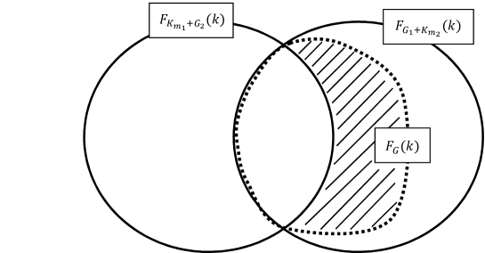
Figure 1. Decomposition of $F_{K_{m}}(k)$

Proof.

Let $V_{1}\sqcup V_{2}$ with $V_{1}=\{v_{1},\ldots,v_{m}\}$ and $V_{2}=\{v_{1}^{\prime},\ldots,v_{m}^{\prime}\}$ denote the common vertex set of $D(G)$, $D(G_{1}+K_{m_{2}})$, $D(K_{m_{1}}+G_{2})$ and $D(K_{m})$ $(=K_{m,m})$. In addition, let $V_{1,1}=\{v_{1},\ldots,v_{m_{1}}\}$, $V_{1,2}=\{v_{m_{1}+1},\ldots,v_{m}\}$, $V_{2,1}=\{v_{1}^{\prime},\ldots,v_{m_{1}}^{\prime}\}$ and $V_{2,2}=\{v_{m_{1}+1}^{\prime},\ldots,v_{m}^{\prime}\}$, where $V_{1,j}\sqcup V_{2,j}$ corresponds to the vertex set of $D(G_{j})$ for $j=1,2$.

Claim 1. $F_{K_{m_{1}}+G_{2}}(k)\subset F_{K_{m}}(k)$.

Suppose that $f$ belongs to $F_{K_{m_{1}}+G_{2}}(k)\cup F_{K_{m}}(k)$. Then condition (ii) in Proposition 2.1 is independent from the value $f(v_{1})$ since $\deg(v_{1})=m$. Thus one can choose $j^{\prime}=1$ for condition (iii) for any $j>1$, and hence we have

$$k=|\{v_{j}\in V_{1}:v_{j}\neq v_{1},f(v_{j})>0\}|.$$

Therefore

(8) $$F_{K_{m_{1}}+G_{2}}(k)\subset F_{K_{m}}(k)$$

and $F_{K_{m_{1}}+G_{2}}(\ell)\cap F_{K_{m}}(k)=\emptyset$ if $\ell\neq k$.

Claim 2. $F_{G}(k)\subset F_{G_{1}+K_{m_{2}}}(k)$.

Suppose that $f\in F_{G}(k)$. Then $f\in F_{G_{1}+K_{m_{2}}}(\ell)$ for some $\ell$. Note that $k=|\eta_{D(G)}(f)|$ and $\ell=|\eta_{D(G_{1}+K_{m_{2}})}(f)|$ (where $\eta$ is defined in Proposition 2.1). In order to prove $k=\ell$, we will show that $\eta_{D(G)}(f)=\eta_{D(G_{1}+K_{m_{2}})}(f)$. Suppose that $f(v_{j})>0$ for $v_{j}\in V_{1}$ ($j\neq 1$). If $j\leq m_{1}+1$, then $v_{j}$ belongs to $\eta_{D(G)}(f)$ if and only if $v_{j}$ belongs to $\eta_{D(G_{1}+K_{m_{2}})}(f)$ since the vertex $v_{j^{\prime}}$ in condition (iii) in Proposition 2.1 should be chosen from $V_{1,1}$. Let $j\geq m_{1}+2$. Since $v_{m_{1}+1}$ belongs to $V_{1,2}$ with $m_{1}+1<j$, (6) holds for $g$ defined in condition (iii) of Proposition 2.1 where $v_{j^{\prime}}=v_{m_{1}+1}$. Thus $v_{j^{\prime}}=v_{m_{1}+1}$ satisfies condition (iii) of Proposition 2.1 for $v_{j}$ in $D(G_{1}+K_{m_{2}})$. Hence $v_{j}$ belongs to $\eta_{D(G_{1}+K_{m_{2}})}(f)$. We now show that any $v_{j}$ ($j\geq m_{1}+2$) belongs to $\eta_{D(G)}(f)$, i.e., there exists $j^{\prime}<j$ such that $g:V_{1}\rightarrow{\mathbb{Z}}_{\geq 0}$ defined by

(9) $$g(v_{i})=\begin{cases}f(v_{i})+1&(i=j^{\prime})\\ f(v_{i})-1&(i=j)\\ f(v_{i})&\mbox{(otherwise)}\end{cases}$$

is a hypertree in $D(G)$. Let $\Gamma$ be a spanning tree of $D(G)$ that induces $f$. Suppose that $\Gamma$ does not contain an edge $e=\{v_{k},v_{1}^{\prime}\}$ for some $m_{1}<k\leq m$. Then $\Gamma\cup\{e\}$ has a unique cycle, and the cycle contains $v_{k}$. Let $e^{\prime}$ be the edge of the cycle that is adjacent to $v_{k}$ but different from $e$. Then $(\Gamma\cup\{e^{\prime}\})\setminus\{e\}$ induces $f$. Thus we may assume that $\{\{v_{k},v_{1}^{\prime}\}:m_{1}<k\leq m\}\subset\Gamma$. By the same argument, we may assume that $\{\{v_{k},v_{m_{1}+1}^{\prime}\}:1\leq k\leq m_{1}\}$ is a subset of $\Gamma$. Hence

$$S=\{\{v_{1},v_{m_{1}+1}^{\prime}\},\ldots,\{v_{m_{1}},v_{m_{1}+1}^{\prime}\},\{v_{m_{1}+1},v_{1}^{\prime}\},\ldots,\{v_{m},v_{1}^{\prime}\}\}$$

is a subset of $\Gamma$. Since $\Gamma$ is spanning,

$$T=\{\{v_{i_{2}},v_{2}^{\prime}\},\ldots,\{v_{i_{m_{1}}},v_{m_{1}}^{\prime}\},\{v_{i_{m_{1}+2}},v_{m_{1}+2}^{\prime}\},\ldots,\{v_{i_{m}},v_{m}^{\prime}\}\}$$

is a subset of $\Gamma$ for some $1\leq i_{2},\ldots,i_{m_{1}},i_{m_{1}+2},\ldots,i_{m}\leq m$. Then $S\cap T=\emptyset$ and $|S\cup T|=2m-2$. Since $\Gamma$ has $2m-1$ edges, we have

$$\Gamma=S\sqcup T\sqcup\{e\}$$

for some edge $e$ of $D(G)$. In particular, the degree of each vertex $v_{i}^{\prime}$ ($i\in[m]\setminus\{1,m_{1}+1\}$) in $\Gamma$ is at most $2$. Since $f(v_{j})>0$, the degree of $v_{j}$ in $\Gamma$ is at least 2, and hence $\{v_{j},v_{k}^{\prime}\}$ is an edge of $\Gamma$ for some $k\in[m]\setminus\{1\}$. Let $e^{\prime}=\{v_{j},v_{k}^{\prime}\}$. We now construct a spanning tree of $D(G)$ that induces a hypertree of the form (9). Note that, for an edge $e^{\prime\prime}$ of $D(G)$, $\Gamma^{\prime}=(\Gamma\cup\{e^{\prime\prime}\})\setminus\{e^{\prime}\}$ is a spanning tree of $D(G)$ if $e^{\prime\prime}\notin\Gamma$ and the (unique) cycle of $\Gamma\cup\{e^{\prime\prime}\}$ contains $e^{\prime}$.

Case A ($k=m_{1}+1$). Then $\Gamma$ contains a path $(v_{1}^{\prime},v_{j},v_{m_{1}+1}^{\prime},v_{1})$. Since $\Gamma$ has no cycles, $\{v_{1},v_{1}^{\prime}\}$ is not an edge of $\Gamma$. Hence $(\Gamma\cup\{v_{1},v_{1}^{\prime}\})\setminus\{e^{\prime}\}$ is a spanning tree of $D(G)$ that induces a hypertree of the form (9) where $j^{\prime}=1$.

Case B ($k\neq m_{1}+1$ and $\deg(v_{k}^{\prime})=1$). If $2\leq k\leq m_{1}$, then $(\Gamma\cup\{v_{k},v_{k}^{\prime}\})\setminus\{e^{\prime}\}$ is a spanning tree of $D(G)$ that induces a hypertree of the form (9) where $j^{\prime}=k$. If $m_{1}+2\leq k\leq m$, then $(\Gamma\cup\{v_{1},v_{k}^{\prime}\})\setminus\{e^{\prime}\}$ is a spanning tree of $D(G)$ that induces a hypertree of the form (9) where $j^{\prime}=1$.

Case C ($k\neq m_{1}+1$ and $\deg(v_{k}^{\prime})=2$). Then $\Gamma$ contains an edge $\{v_{\ell},v_{k}^{\prime}\}$ for some $\ell\neq j$. If $m_{1}<\ell\leq m$, then $\Gamma$ contains a cycle $(v_{1}^{\prime},v_{j},v_{k}^{\prime},v_{\ell},v_{1}^{\prime})$ of length 4. This is a contradiction. Hence $\ell\leq m_{1}$. Then $\Gamma$ contains a path $(v_{1}^{\prime},v_{j},v_{k}^{\prime},v_{\ell},v_{m_{1}+1}^{\prime},v_{1})$. Since $\Gamma$ has no cycles, $\{v_{1},v_{1}^{\prime}\}$ is not an edge of $\Gamma$. Hence $(\Gamma\cup\{v_{1},v_{1}^{\prime}\})\setminus\{e^{\prime}\}$ is a spanning tree of $D(G)$ that induces a hypertree of the form (9) where $j^{\prime}=1$.

Thus we have $k=\ell$, and hence

(10) $$F_{G}(k)\subset F_{G_{1}+K_{m_{2}}}(k).$$

Claim 3. $(F_{G_{1}+K_{m_{2}}}(k)\setminus F_{G}(k))\subset F_{K_{m}}(k)$.

Suppose that $f$ belongs to $F_{G_{1}+K_{m_{2}}}(k)\setminus F_{G}(k)$. Then there exists $V^{\prime}\subset V_{1,2}$ such that

$$\sum_{v\in V^{\prime}}f(v)\geq|\Gamma_{D(G_{2})}(V^{\prime})|+m_{1}.$$

In particular, $\sum_{v\in V_{1,2}}f(v)>m_{1}$. Since $\sum_{v\in V_{1}}f(v)=m-1$, we have $\sum_{v\in V_{1,1}}f(v)<m_{2}-1$. Hence

$$\sum_{v\in V^{\prime\prime}}f(v)<m_{2}-1<|\Gamma_{D(G_{1})}(V^{\prime\prime})|+m_{2}-1$$

for all $V^{\prime\prime}\subset V_{1,1}$. Thus, for each $v_{j}\neq v_{1}$ with $f(v_{j})>0$, $g:V_{1}\rightarrow{\mathbb{Z}}_{\geq 0}$ defined by

$$g(v_{i})=\begin{cases}f(v_{i})+1&(i=1)\\ f(v_{i})-1&(i=j)\\ f(v_{i})&\mbox{(otherwise)}\end{cases}$$

satisfies

$$\sum_{v\in V^{\prime\prime}}g(v)\leq 1+\sum_{v\in V^{\prime\prime}}f(v)\leq|\Gamma_{D(G_{1})}(V^{\prime\prime})|+m_{2}-1$$

for all $V^{\prime\prime}\subset V_{1,1}$. Therefore we have

$$k=|\{v_{j}\in V_{1}:v_{j}\neq v_{1},f(v_{j})>0\}|,$$

and hence

(11) $$(F_{G_{1}+K_{m_{2}}}(k)\setminus F_{G}(k))\subset F_{K_{m}}(k).$$

Claim 4. $F_{K_{m}}(k)=F_{K_{m_{1}}+G_{2}}(k)\cup(F_{G_{1}+K_{m_{2}}}(k)\setminus F_{G}(k))$.

From (8) and (11),

$$F_{K_{m}}(k)\supset F_{K_{m_{1}}+G_{2}}(k)\cup(F_{G_{1}+K_{m_{2}}}(k)\setminus F_{G}(k)).$$

Let $f\in F_{K_{m}}(k)\setminus F_{K_{m_{1}}+G_{2}}(k)$. Since $F_{K_{m_{1}}+G_{2}}(k^{\prime})\cap F_{K_{m}}(k)=\emptyset$ for any $k^{\prime}\neq k$, it follows that $f\notin F_{K_{m_{1}}+G_{2}}(\ell)$ for any $\ell$. Hence from (5), $f\in F_{G_{1}+K_{m_{2}}}(\ell)$ for some $\ell$. If $f\in F_{G}(\ell)$, then $f\in F_{K_{m_{1}}+G_{2}}(\ell^{\prime})$ for some $\ell^{\prime}$ by (4). This is a contradiction. Thus $f\in F_{G_{1}+K_{m_{2}}}(\ell)\setminus F_{G}(\ell)$. From (11), we have

$$f\in F_{G_{1}+K_{m_{2}}}(\ell)\setminus F_{G}(\ell)\subset F_{K_{m}}(\ell).$$

Then $\ell=k$. It follows that

$$F_{K_{m}}(k)=F_{K_{m_{1}}+G_{2}}(k)\cup(F_{G_{1}+K_{m_{2}}}(k)\setminus F_{G}(k)).$$

Finally, we show that this is a decomposition. Suppose that $f\in F_{G_{1}+K_{m_{2}}}(k)\cap F_{K_{m_{1}}+G_{2}}(k)$. From (4), $f\in F_{G}(\ell)$ for some $\ell$. Moreover, from (10), we have $\ell=k$. Thus

$$F_{G_{1}+K_{m_{2}}}(k)\cap F_{K_{m_{1}}+G_{2}}(k)\subset F_{G}(k).$$

Therefore $F_{K_{m}}(k)$ is decomposed into the disjoint sets

$$F_{K_{m}}(k)=F_{K_{m_{1}}+G_{2}}(k)\sqcup(F_{G_{1}+K_{m_{2}}}(k)\setminus F_{G}(k))$$

as in Fig. 1. ∎

Now, we are in the position to give a proof of Theorem 1.1.

Proof of Theorem 1.1.

We prove this by induction on $s$. First we discuss the case when $s=2$, i.e., $G=G_{1}+G_{2}$. It is known [12, Example 5.3] that

$$|F_{K_{m}}(k)|=\binom{m-1}{k}^{2}.$$

From Lemma 3.2,

$$\binom{m-1}{k}^{2}=|F_{K_{m_{1}}+G_{2}}(k)|+(|F_{G_{1}+K_{m_{2}}}(k)|-|F_{G}(k)|).$$

Thus we have

$$I_{D(G)}(x)=I_{D(G_{1}+K_{m_{2}})}(x)+I_{D(G_{2}+K_{m_{1}})}(x)-\sum_{k=0}^{m-1}\binom{m-1}{k}^{2}x^{k}.$$

Let $s>2$ and assume that the assertion holds for the join of at most $s-1$ graphs. Since $G=(G_{1}+\cdots+G_{s-1})+G_{s}$, we have

$$I_{D(G)}(x) = I_{D((G_{1}+\cdots+G_{s-1})+K_{m_{s}})}(x)+I_{D(G_{s}+K_{m-m_{s}})}(x)-\sum_{k=0}^{m-1}\binom{m-1}{k}^{2}x^{k}$$

$$= \sum_{i=1}^{s-2}I_{D(G_{i}+K_{m-m_{i}})}(x)+I_{D((G_{s-1}+K_{m_{s}})+K_{m-m_{s-1}-m_{s}})}(x)$$

$$-(s-2)\sum_{k=0}^{m-1}\binom{m-1}{k}^{2}x^{k}+I_{D(G_{s}+K_{m-m_{s}})}(x)-\sum_{k=0}^{m-1}\binom{m-1}{k}^{2}x^{k}$$

$$= \sum_{i=1}^{s}I_{D(G_{i}+K_{m-m_{i}})}(x)-(s-1)\sum_{k=0}^{m-1}\binom{m-1}{k}^{2}x^{k}.$$

From Proposition 2.4 and Lemma 2.5, this is equal to equation (3). ∎

4. Complete multipartite graphs

In this section, applying Theorem 1.1, we give explicit formulas for the $h^{*}$-polynomial and the normalized volume of the PQ-type adjacency polytope of a complete multipartite graph.

Given positive integers $\ell$ and $m$, let

$$f_{\ell,m}(x)=\sum_{k=0}^{\ell+m-1}\sum_{\alpha=0}^{k}\binom{\ell-1}{k-\alpha}\binom{m}{\alpha}\sum_{\beta=\alpha}^{k}\binom{\ell+\alpha-1}{\beta}\binom{m-\alpha}{k-\beta}x^{k}.$$

Since

$$\sum_{k=0}^{\ell+m-1}\sum_{\alpha=0}^{k}\binom{\ell-1}{k-\alpha}\binom{m}{\alpha}\sum_{\beta=0}^{k}\binom{\ell+\alpha-1}{\beta}\binom{m-\alpha}{k-\beta}x^{k}$$

$$= \sum_{k=0}^{\ell+m-1}\sum_{\alpha=0}^{k}\binom{\ell-1}{k-\alpha}\binom{m}{\alpha}\binom{\ell+m-1}{k}x^{k}$$

$$= \sum_{k=0}^{\ell+m-1}\binom{\ell+m-1}{k}\sum_{\alpha=0}^{k}\binom{\ell-1}{k-\alpha}\binom{m}{\alpha}x^{k}$$

$$= \sum_{k=0}^{\ell+m-1}\binom{\ell+m-1}{k}^{2}x^{k}$$

holds, we have

$$f_{\ell,m}(x)=\sum_{k=0}^{\ell+m-1}\binom{\ell+m-1}{k}^{2}x^{k}-\sum_{k=1}^{m-1}\sum_{\alpha=1}^{k}\binom{\ell-1}{k-\alpha}\binom{m}{\alpha}\sum_{\beta=0}^{\alpha-1}\binom{\ell+\alpha-1}{\beta}\binom{m-\alpha}{k-\beta}x^{k}.$$

The $h^{*}$-polynomial of $\nabla_{G}^{\rm PQ}$ for the graph $G=K_{\ell}+E_{m}$ $(=K_{1,\dots,1,m})$ coincides with $f_{\ell,m}(x)$.

Theorem 4.1.

Let $G=K_{\ell}+E_{m}$. Then we have

$$h^{*}(\nabla_{G}^{\rm PQ},x) = f_{\ell,m}(x),$$

$${\rm Vol}(\nabla_{G}^{\rm PQ}) = f_{\ell,m}(1)=\sum_{\alpha=0}^{m}\binom{m}{\alpha}\sum_{\beta=0}^{\ell-1}\binom{\ell+\alpha-1}{\beta}\binom{\ell+m-\alpha-1}{\beta}.$$

Proof.

Let $G^{\prime}=D(K_{\ell-1}+E_{m})$. Since $G=(K_{\ell-1}+E_{m})+K_{1}$, from Proposition 2.6, we have

$$h^{*}(\nabla_{G}^{\rm PQ},x)=p(G^{\prime},x)=\sum_{k=0}^{\ell+m-1}\left|{\rm PM}(G^{\prime},k)\right|x^{k}.$$

Let $n=\ell+m-1$ and let $[n]\cup[\overline{n}]$ be the vertex set of $G^{\prime}$. We decompose $[n]$ into two disjoint set $V_{1,1}=[\ell-1]$ and $V_{1,2}=[n]\setminus[\ell-1]$ where $V_{1,1}$ (resp. $V_{1,2}$) corresponds to $K_{\ell-1}$ (resp. $E_{m}$). From Proposition 2.8, each $|{\rm PM}(G^{\prime},k)|$ is the number of $(0,1)$-vectors $(x_{1},\ldots,x_{n},y_{1},\ldots,y_{n})\in{\mathbb{R}}^{2n}$ such that

(12) $$\sum_{i=1}^{n}x_{i} = \sum_{i=1}^{n}y_{i}=k,$$

(13) $$\sum_{i\in S}x_{i} \leq \sum_{\overline{j}\in\Gamma_{G^{\prime}}(S)}y_{j}\ \ \mbox{ for all }S\subset[n].$$

If (12) holds and a subset $S\subset[n]$ contains an element of $V_{1,1}$, then we have $\Gamma_{G^{\prime}}(S)=[\overline{n}]$, and hence

$$\sum_{\overline{j}\in\Gamma_{G^{\prime}}(S)}y_{j}=k=\sum_{i=1}^{n}x_{i}\geq\sum_{i\in S}x_{i}.$$

Thus (12) and (13) hold if and only if

(14) $$\sum_{i=1}^{n}x_{i} = \sum_{i=1}^{n}y_{i}=k,$$

(15) $$\sum_{i\in S}x_{i} \leq \sum_{\overline{j}\in\Gamma_{G^{\prime}}(S)}y_{j}\ \ \mbox{ for all }S\subset V_{1,2}.$$

We count such vectors with $|\{i\in V_{1,2}:x_{i}=1\}|=\alpha$ for each $\alpha=0,1,\ldots,k$. There are $\binom{m}{\alpha}$ possibilities for the choice of the subset $S^{\prime}=\{i\in V_{1,2}:x_{i}=1\}\subset V_{1,2}$. For each $S^{\prime}$, there are $\binom{\ell-1}{k-\alpha}$ possibilities for the choice of the subset $\{i\in V_{1,1}:x_{i}=1\}\subset V_{1,1}$. Then equations (14) and (15) hold if and only if $\sum_{i=1}^{n}y_{i}=k$ and $\alpha\leq\sum_{\overline{j}\in\Gamma_{G^{\prime}}(S^{\prime})}y_{j}$. Let $\beta=\sum_{\overline{j}\in\Gamma_{G^{\prime}}(S^{\prime})}y_{j}$. Since $|\Gamma_{G^{\prime}}(S^{\prime})|=\ell+\alpha-1$, there are $\binom{\ell+\alpha-1}{\beta}$ possibilities for the choice of the subset $S^{\prime\prime}=\{\overline{j}\in\Gamma_{G^{\prime}}(S^{\prime}):y_{j}=1\}\subset\Gamma_{G^{\prime}}(S^{\prime})$. For each $S^{\prime\prime}$, there are $\binom{m-\alpha}{k-\beta}$ possibilities for the choice of the subset $\{\overline{j}\in[\overline{n}]\setminus\Gamma_{G^{\prime}}(S^{\prime}):y_{j}=1\}\subset[\overline{n}]\setminus\Gamma_{G^{\prime}}(S^{\prime})$. Thus we have $I_{D(G)}(x)=f_{\ell,m}(x)$.

Moreover, the normalized volume of $\nabla_{G}^{\rm PQ}$ is equal to

$$f_{\ell,m}(1) = \sum_{k=0}^{\ell+m-1}\sum_{\alpha=0}^{k}\binom{\ell-1}{k-\alpha}\binom{m}{\alpha}\sum_{\beta=\alpha}^{k}\binom{\ell+\alpha-1}{\beta}\binom{m-\alpha}{k-\beta}$$

$$= \sum_{\alpha=0}^{m}\binom{m}{\alpha}\sum_{\beta=\alpha}^{\ell+\alpha-1}\binom{\ell+\alpha-1}{\beta}\sum_{k=\beta}^{\ell+\alpha-1}\binom{\ell-1}{k-\alpha}\binom{m-\alpha}{k-\beta}$$

$$= \sum_{\alpha=0}^{m}\binom{m}{\alpha}\sum_{\beta=\alpha}^{\ell+\alpha-1}\binom{\ell+\alpha-1}{\beta}\sum_{k=\beta}^{\ell+\alpha-1}\binom{\ell-1}{\ell-1+\alpha-\beta-(k-\beta)}\binom{m-\alpha}{k-\beta}$$

$$= \sum_{\alpha=0}^{m}\binom{m}{\alpha}\sum_{\beta=\alpha}^{\ell+\alpha-1}\binom{\ell+\alpha-1}{\beta}\binom{\ell+m-\alpha-1}{\ell+\alpha-\beta-1}$$

$$= \sum_{\alpha=0}^{m}\binom{m}{\alpha}\sum_{\beta^{\prime}=0}^{\ell-1}\binom{\ell+\alpha-1}{\beta^{\prime}}\binom{\ell+m-\alpha-1}{\beta^{\prime}}.$$

∎

Remark 4.2.

Let $G=K_{\ell}+E_{m}$. Since

$$\sum_{\alpha=0}^{m}\binom{m}{\alpha}\sum_{\beta=0}^{\ell+\alpha-1}\binom{\ell+\alpha-1}{\beta}\binom{\ell+m-\alpha-1}{\beta}=\binom{2(\ell+m-1)}{\ell+m-1},$$

we have

$${\rm Vol}(\nabla_{G}^{\rm PQ})=\binom{2(\ell+m-1)}{\ell+m-1}-\sum_{\alpha=1}^{m-1}\binom{m}{\alpha}\sum_{\beta=\ell}^{\ell+\alpha-1}\binom{\ell+\alpha-1}{\beta}\binom{\ell+m-\alpha-1}{\beta}.$$

Example 4.3.

For small $\ell$ and $m$, $f_{\ell,m}(1)$ in Theorem 4.1 is

$$f_{1,m}(1) = 2^{m},$$

$$f_{2,m}(1) = 2^{m-2}\left(m^{2}+3m+8\right),$$

$$f_{3,m}(1) = \frac{2^{m-4}}{(2!)^{2}}\left(m^{4}+10m^{3}+59m^{2}+186m+384\right),$$

$$f_{4,m}(1) = \frac{2^{m-6}}{(3!)^{2}}\left(m^{6}+21m^{5}+229m^{4}+1563m^{3}+7762m^{2}+24984m+46080\right),$$

$$f_{\ell,1}(1) = \binom{2\ell}{\ell},$$

$$f_{\ell,2}(1) = \binom{2(\ell+1)}{\ell+1}-2,$$

$$f_{\ell,3}(1) = \binom{2(\ell+2)}{\ell+2}-(6\ell+6),$$

$$f_{\ell,4}(1) = \binom{2(\ell+3)}{\ell+3}-(10\ell^{2}+24\ell+20).$$

From Theorems 1.1 and 4.1, we have the following.

Corollary 4.4.

Let $G$ be a complete multipartite graph $K_{m_{1},\dots,m_{s}}$, and let $m=\sum_{i=1}^{s}m_{i}$. Then we have

$$h^{*}(\nabla_{G}^{\rm PQ},x) = \sum_{i=1}^{s}f_{m-m_{i},m_{i}}(x)-(s-1)\sum_{k=0}^{m-1}\binom{m-1}{k}^{2}x^{k},$$

$${\rm Vol}(\nabla_{G}^{\rm PQ}) = \sum_{i=1}^{s}f_{m-m_{i},m_{i}}(1)-(s-1)\binom{2(m-1)}{m-1}.$$

Example 4.5.

From Corollary 4.4, the normalized volume of $\nabla_{K_{\ell,m}}^{\rm PQ}$ is

$$f_{\ell,m}(1)+f_{m,\ell}(1)-\binom{2(\ell+m-1)}{\ell+m-1}.$$

From Example 4.3, we have

$${\rm Vol}(\nabla_{K_{1,m}}^{\rm PQ}) = 2^{m},$$

$${\rm Vol}(\nabla_{K_{2,m}}^{\rm PQ}) = 2^{m-2}\left(m^{2}+3m+8\right)-2,$$

$${\rm Vol}(\nabla_{K_{3,m}}^{\rm PQ}) = \frac{2^{m-4}}{(2!)^{2}}\left(m^{4}+10m^{3}+59m^{2}+186m+384\right)-(6m+6),$$

$${\rm Vol}(\nabla_{K_{4,m}}^{\rm PQ}) = \frac{2^{m-6}}{(3!)^{2}}\left(m^{6}+21m^{5}+229m^{4}+1563m^{3}+7762m^{2}+24984m+46080\right)$$

$$-(10m^{2}+24m+20).$$

The formula for ${\rm Vol}(\nabla_{K_{2,m}}^{\rm PQ})$ coincides with that in [8, Proposition 4.2].

Example 4.6.

Let $G$ be the complete bipartite graph $K_{2,n-2}$. Since

$$f_{2,m}(x) = \sum_{k=0}^{m+1}\sum_{\alpha=0}^{k}\binom{1}{k-\alpha}\binom{m}{\alpha}\sum_{\beta=\alpha}^{k}\binom{\alpha+1}{\beta}\binom{m-\alpha}{k-\beta}x^{k}$$

$$= \sum_{k=0}^{m+1}\binom{m}{k-1}k(m-k+1)x^{k}+\sum_{k=0}^{m+1}\binom{m}{k-1}x^{k}+\sum_{k=0}^{m+1}\binom{m}{k}(k+1)x^{k}$$

$$= \sum_{k=0}^{m}\binom{m}{k}k^{2}x^{k}+\sum_{k=0}^{m}\binom{m}{k}x^{k+1}+\sum_{k=0}^{m}\binom{m}{k}(k+1)x^{k}$$

$$= \sum_{k=0}^{m}\binom{m}{k}(x+1+k^{2}+k)x^{k}$$

$$= (x+1)^{m+1}+m\left((m+1)x+2\right)x(x+1)^{m-2}$$

and

$$f_{\ell,2}(x) = \sum_{k=0}^{\ell+1}\binom{\ell+1}{k}^{2}x^{k}-2x,$$

we have

$$h^{*}(\nabla_{G}^{\rm PQ},x) = f_{2,n-2}(x)+f_{n-2,2}(x)-\sum_{k=0}^{n-1}\binom{n-1}{k}^{2}x^{k}$$

$$= (x+1)^{n-1}+(n-2)\left((n-1)x+2\right)x(x+1)^{n-4}-2x.$$

5. Wheel graphs

For $n\geq 3$, the wheel graph $W_{n}$ with $n+1$ vertices is the join graph $W_{n}=C_{n}+K_{1}$. Unfortunately, Theorem 1.1 is not useful for computing the $h^{*}$-polynomial of $\nabla_{W_{n}}^{\rm PQ}$. We will give an explicit formula for the $h^{*}$-polynomial of $\nabla_{W_{n}}^{\rm PQ}$ and prove the conjecture [8, Conjecture 4.4] on the normalized volume of $\nabla_{W_{n}}^{\rm PQ}$ by using Proposition 2.6 on $\nabla_{G+K_{1}}^{\rm PQ}$.

Let

$$\gamma(n,x)=\left\{\begin{array}[]{ll}1&\mbox{if }n=0,\\ \\ \frac{(1+\sqrt{1+8x})^{n}+(1-\sqrt{1+8x})^{n}}{2^{n}}&\mbox{if }n\mbox{ is odd,}\\ \\ \frac{(1+\sqrt{1+8x})^{n}+(1-\sqrt{1+8x})^{n}}{2^{n}}-2x^{\frac{n}{2}}&\mbox{otherwise}.\end{array}\right.$$

For $n\geq 3$,

$$\frac{(1+\sqrt{1+8x})^{n}+(1-\sqrt{1+8x})^{n}}{2^{n}}=g(C_{n},2x),$$

where $g(C_{n},x)$ is the matching generating polynomial of $C_{n}$. Moreover, for $n\geq 3$, it is known [16, Example 4.5] that, $\gamma(n,x)$ is the $\gamma$-polynomial of the PV-type adjacency polytope $\nabla^{\rm PV}_{W_{n}}$ of $W_{n}$. (Note that $\nabla^{\rm PV}_{W_{n}}$ is called the symmetric edge polytope of type A of $W_{n}$ in [16].) The $h^{*}$-polynomial of $\nabla_{W_{n}}^{\rm PQ}$ is described by this function as follows.

Theorem 5.1.

The $h^{*}$-polynomial of $\nabla_{W_{n}}^{\rm PQ}$ is

$$\sum_{k=0}^{n}\binom{n}{k}\gamma(n-k,x)x^{k}$$

$$= \left(\frac{1+2x+\sqrt{1+8x}}{2}\right)^{n}+\left(\frac{1+2x-\sqrt{1+8x}}{2}\right)^{n}+x^{n}-(x+\sqrt{x})^{n}-(x-\sqrt{x})^{n}.$$

Moreover, the normalized volume of $\nabla_{W_{n}}^{\rm PQ}$ is $3^{n}-2^{n}+1$.

Proof.

Since $W_{n}=C_{n}+K_{1}$, the $h^{*}$-polynomial of $\nabla_{W_{n}}^{\rm PQ}$ is

$$p(D(C_{n}),x)=\sum_{\ell=0}^{n}|{\rm PM}(D(C_{n}),\ell)|x^{\ell}$$

by Proposition 2.6. From Proposition 2.8, $|{\rm PM}(D(C_{n}),\ell)|$ is equal to the number of $(0,1)$-vectors $(x_{1},\ldots,x_{n},y_{1},\ldots,y_{n})\in{\mathbb{R}}^{2n}$ such that

(16) $$\sum_{i=1}^{n}x_{i} = \sum_{j=1}^{n}y_{j}=\ell,$$

(17) $$\sum_{i\in S}x_{i} \leq \sum_{\overline{j}\in\Gamma_{G^{\prime}}(S)}y_{j}\ \ \mbox{ for all }S\subset[n],$$

where $V=[n]\cup[\overline{n}]$ is the set of vertices of $D(C_{n})$. Let $C_{n}=(1,2,\dots,n,1)$. Given a subset $T\subset[n]$ and an integer $\ell\in[n]$, let ${\rm PM}_{T,\ell}$ denote the set of all $(0,1)$ vectors $(x_{1},\ldots,x_{n},y_{1},\ldots,y_{n})\in{\mathbb{R}}^{2n}$ satisfying (16), (17), and $T=\{i\in[n]:x_{i}=y_{i}=1\}$. Note that ${\rm PM}_{T,\ell}=\emptyset$ if $\ell<|T|$.

Let $T\subset[n]$ with $|T|=k$. We will show that $\sum_{\ell=k}^{n}|{\rm PM}_{T,\ell}|x^{\ell}=\gamma(n-k,x)x^{k}$.

Case 1 ($k=n$). It is easy to see that ${\rm PM}_{T,n}=\{(1,\dots,1)\}$ and ${\rm PM}_{T,\ell}=\emptyset$ if $\ell\neq n$. Note that $\gamma(n-k,x)x^{k}=x^{n}$ if $k=n$. Thus $\sum_{\ell=k}^{n}|{\rm PM}_{T,\ell}|x^{\ell}=\gamma(n-k,x)x^{k}$.

Case 2 ($k=n-1$). Let $T=[n]\setminus\{i\}$ where $i\in[n]$. It then follows that ${\rm PM}_{T,n-1}=\{(1,\dots,1)-{\bf e}_{i}-{\bf e}_{n+i}\}$ and ${\rm PM}_{T,\ell}=\emptyset$ if $\ell\neq n-1$. Note that $\gamma(n-k,x)x^{k}=x^{n-1}$ if $k=n-1$. Thus $\sum_{\ell=k}^{n}|{\rm PM}_{T,\ell}|x^{\ell}=\gamma(n-k,x)x^{k}$.

Case 3 ($k=n-2$). Let $T=[n]\setminus\{i,j\}$ where $1\leq i<j\leq n$. Since (16) holds, each element of ${\rm PM}_{T,\ell}$ is

$$\alpha_{1}=(1,\dots,1)-{\bf e}_{i}-{\bf e}_{j}-{\bf e}_{n+i}-{\bf e}_{n+j}$$

if $\ell=n-2$, and is one of

$$\alpha_{2} = (1,\dots,1)-{\bf e}_{i}-{\bf e}_{n+j},$$

$$\alpha_{3} = (1,\dots,1)-{\bf e}_{j}-{\bf e}_{n+i},$$

if $\ell=n-1$. Then each $\alpha_{i}$ corresponds to a perfectly matchable set. In fact, a matching of $D(C_{n})$ which corresponds to $\alpha_{1}$, $\alpha_{2}$, $\alpha_{3}$ is

$$\{\{s,\overline{s}\}:s\in[n]\setminus\{i,j\}\},$$

$$\{\{s,\overline{s}\}:1\leq s\leq i-1\mbox{ or }j+1\leq s\leq n\}\cup\{\{s+1,\overline{s}\}:i\leq s\leq j-1\},$$

$$\{\{s,\overline{s}\}:1\leq s\leq i-1\mbox{ or }j+1\leq s\leq n\}\cup\{\{s,\overline{s+1}\}:i\leq s\leq j-1\},$$

respectively. Thus

$${\rm PM}_{T,\ell}=\left\{\begin{array}[]{cc}\{\alpha_{1}\}&\mbox{if }\ell=n-2,\\ \\ \{\alpha_{2},\alpha_{3}\}&\mbox{if }\ell=n-1,\\ \\ \emptyset&\mbox{otherwise}.\end{array}\right.$$

Note that $\gamma(n-k,x)x^{k}=(2x+1)x^{n-2}=x^{n-2}+2x^{n-1}$ if $k=n-2$. Thus $\sum_{\ell=k}^{n}|{\rm PM}_{T,\ell}|x^{\ell}=\gamma(n-k,x)x^{k}$.

Case 4 ($k\leq n-3$). Suppose that $T^{\prime}=\{p,p+1,\dots,q\}\subset T$ and $p-1,q+1\notin T$. Since $|T|\leq n-3$, we have $n-q+p-1\geq 3$. Let $U=\{p,p+1,\dots,q,\overline{p},\overline{p+1},\dots,\overline{q}\}$. We will show that there exists a perfectly matchable set $S$ of $D(C_{n-q+p-1})$ such that

$$\rho(S)=(x_{1},\ldots,x_{p-1},x_{q+1},\dots,x_{n},y_{1},\ldots,y_{p-1},y_{q+1},\dots,y_{n})$$

for any $(x_{1},\dots,x_{n},y_{1},\dots,y_{n})\in{\rm PM}_{T,\ell}$. Here $C_{n-q+p-1}=(1,\ldots,p-1,q+1,\ldots,n,1)$ and the vertex set of $D(C_{n-q+p-1})$ is $\{1,\ldots,p-1,q+1,\ldots,n\}\cup\{\overline{1},\ldots,\overline{p-1},\overline{q+1},\ldots,\overline{n}\}$. Let $M$ be a matching of $D(C_{n})$ which corresponds to $(x_{1},\dots,x_{n},y_{1},\dots,y_{n})$.

Case 4.1 (either $x_{p-1}=x_{q+1}=0$ or $y_{p-1}=y_{q+1}=0$). Exchanging $[n]$ and $[\overline{n}]$ if needed, we may assume that $y_{p-1}=y_{q+1}=0$. Then, for the subset $T^{\prime}\subset[n]$,

$$\sum_{i\in T^{\prime}}x_{i}=\sum_{\overline{j}\in\Gamma_{G^{\prime}}(T^{\prime})}y_{j}=|T^{\prime}|.$$

Hence the matching $M$ is the union of a perfect matching of the induced subgraph $D(C_{n})_{U}$ of $D(C_{n})$ and a matching $M^{\prime}$ of the induced subgraph $D(C_{n})_{V\setminus U}$ of $D(C_{n})$. Then one can regard $M^{\prime}$ as a matching of $D(C_{n-q+p-1})$ since $D(C_{n})_{V\setminus U}$ is a subgraph of $D(C_{n-q+p-1})$.

Case 4.2 ($x_{p-1}=y_{q+1}\neq y_{p-1}=x_{q+1}$). Exchanging $[n]$ and $[\overline{n}]$ if needed, we may assume that $x_{p-1}=y_{q+1}=1$ and $y_{p-1}=x_{q+1}=0$. If $e=\{q+2,\overline{q+1}\}$ belongs to the matching $M$, then $M\setminus\{e\}$ is the union of a perfect matching of $D(C_{n})_{U}$ and a matching $M^{\prime}$ of $D(C_{n})_{V\setminus U}$ by the same argument in Case 4.1. Suppose that $e=\{q,\overline{q+1}\}$ belongs to the matching $M$. It then follows that $M$ is the union of $\{\{p-1,\overline{p}\},\ldots,\{q-1,\overline{q}\},\{q,\overline{q+1}\}\}$ and a matching $M^{\prime}$ of $D(C_{n})_{V\setminus U}$. Thus one can regard $M^{\prime}\cup\{\{p-1,\overline{q+1}\}\}$ as a matching of $D(C_{n-q+p-1})$.

Thus there exists a perfectly matchable set $S_{1}$ of $D(C_{n-q+p-1})$ such that

$$\rho(S_{1})=(x_{1},\ldots,x_{p-1},x_{q+1},\dots,x_{n},y_{1},\ldots,y_{p-1},y_{q+1},\dots,y_{n})$$

for $(x_{1},\dots,x_{n},y_{1},\dots,y_{n})$ if $T^{\prime}=\{p,p+1,\dots,q\}\subset T$ and $p-1,q+1\notin T$. If, in addition, $T^{\prime\prime}=\{p^{\prime},p^{\prime}+1,\dots,q^{\prime}\}\subset T$ and $p^{\prime}-1,q^{\prime}+1\notin T$ for some $p^{\prime}>q+1$, then there exists a perfectly matchable set $S_{2}$ of $D(C_{n-(q-p+1)-(q^{\prime}-p^{\prime}+1)})$ such that

$$\rho(S_{2})=(x_{1},\ldots,x_{p-1},x_{q+1},\dots,x_{p^{\prime}-1},x_{q^{\prime}+1},\dots,x_{n},y_{1},\ldots,y_{p-1},y_{q+1},\dots,y_{p^{\prime}-1},y_{q^{\prime}+1},\dots,y_{n})$$

by the same argument as above. Repeating the above argument, it follows that there exists a perfectly matchable set $S$ of $D(C_{n-k})$ such that $\rho(S)=(x_{i_{1}},\ldots,x_{i_{n-k}},y_{i_{1}},\ldots,y_{i_{n-k}})$ where $[n]\setminus T=\{i_{1},\ldots,i_{n-k}\}$ and $x_{i_{r}}+y_{i_{r}}\leq 1$ for all $r$. Then there exists a perfectly matchable set $S^{\prime}$ of $C_{n-k}$ such that $|S^{\prime}|=2(\ell-k)$ and $\rho(S^{\prime})=(x_{i_{1}}+y_{i_{1}},\ldots,x_{i_{n-k}}+y_{i_{n-k}})$. The matching corresponding to $S^{\prime}$ is not unique if and only if $n-k$ is even and $\rho(S^{\prime})=(1,\dots,1)$. There exist two matchings for the perfectly matchable set $S$ of $D(C_{n-k})$ exactly when

$$(x_{i_{1}},\ldots,x_{i_{n-k}},y_{i_{1}},\ldots,y_{i_{n-k}})=(1,0,\ldots,1,0,0,1,\ldots,0,1),(0,1,\ldots,0,1,1,0,\ldots,1,0).$$

Conversely, for each matching $M$ of $C_{n-k}$, there exist $2^{|M|}$ vectors $(x_{i_{1}},\ldots,x_{i_{n-k}},y_{i_{1}},\ldots,y_{i_{n-k}})$ where $x_{i_{r}}+y_{i_{r}}\leq 1$ for all $r$ and associated with a perfectly matchable set of $D(C_{n-k})$ since there are two possibilities $(x_{i_{p}},x_{i_{p+1}},y_{i_{p}},y_{i_{p+1}})=(1,0,0,1),(0,1,1,0)$ for each $\{i_{p},i_{p+1}\}\in M$.

Hence we have

$$|{\rm PM}_{T,\ell}|=\left\{\begin{array}[]{ll}2^{\ell-k}m_{C_{n-k}}(\ell-k)-2&\mbox{if }\ell-k=(n-k)/2,\\ \\ 2^{\ell-k}m_{C_{n-k}}(\ell-k)&\mbox{otherwise}.\end{array}\right.$$

Recall that $m_{G}(k)$ is the number of $k$-matchings of a graph $G$. Thus

$$\sum_{\ell=k}^{n}|{\rm PM}_{T,\ell}|x^{\ell} = \sum_{\ell=k}^{n}2^{\ell-k}m_{C_{n-k}}(\ell-k)x^{\ell}-2x^{(n+k)/2}$$

$$= \left(\sum_{\ell=k}^{n}m_{C_{n-k}}(\ell-k)(2x)^{\ell-k}-2x^{(n-k)/2}\right)x^{k}$$

$$= \gamma(n-k,x)x^{k}$$

if $n-k$ is even, and

$$\sum_{\ell=k}^{n}|{\rm PM}_{T,\ell}|x^{\ell} = \sum_{\ell=k}^{n}2^{\ell-k}m_{C_{n-k}}(\ell-k)x^{\ell}$$

$$= \left(\sum_{\ell=k}^{n}m_{C_{n-k}}(\ell-k)(2x)^{\ell-k}\right)x^{k}$$

$$= \gamma(n-k,x)x^{k}$$

if $n-k$ is odd.

Therefore the $h^{*}$-polynomial of $\nabla_{W_{n}}^{\rm PQ}$ is

$$\sum_{T\subset[n]}\sum_{\ell=|T|}^{n}|{\rm PM}_{T,\ell}|x^{\ell}=\sum_{T\subset[n]}\gamma(n-|T|)x^{|T|}=\sum_{k=0}^{n}\binom{n}{k}\gamma(n-k,x)x^{k}.$$

Moreover

$$\sum_{k=0}^{n}\binom{n}{k}\gamma(n-k,x)x^{k}$$

$$= x^{n}+\sum_{k=0}^{n}\binom{n}{k}\left(\frac{1+\sqrt{1+8x}}{2}\right)^{n-k}x^{k}+\sum_{k=0}^{n}\binom{n}{k}\left(\frac{1-\sqrt{1+8x}}{2}\right)^{n-k}x^{k}$$

$$-\sum_{\begin{subarray}{c}k\geq 0\\ k\equiv n\ (\mbox{\small mod }2)\end{subarray}}2\binom{n}{k}\sqrt{x}^{n-k}x^{k}$$

$$= \left(\frac{1+2x+\sqrt{1+8x}}{2}\right)^{n}+\left(\frac{1+2x-\sqrt{1+8x}}{2}\right)^{n}+x^{n}-(x+\sqrt{x})^{n}-(x-\sqrt{x})^{n}.$$

In particular, substituting $x=1$, we have

$$\sum_{k=0}^{n}\binom{n}{k}\gamma(n-k,1)=3^{n}-2^{n}+1.$$

∎

References

- [1] F. Ardila, M. Back, S, Hoşten, J. Pfeifle and K. Seashore, Root Polytopes and Growth Series of Root Lattices, SIAM J. Discrete Math. 25 (2011), 360–378.
- [2] E. Balas and W.R. Pulleyblank, The perfectly matchable subgraph polytopes of a bipartite graph, Networks 13 (1983), 495–516.
- [3] E. Balas and W.R. Pulleyblank, The perfectly matchable subgraph polytope of an arbitrary graph, Combinatorica 9 (1989), 321–337.
- [4] M. Beck and S. Robins, “Computing the continuous discretely”, Undergraduate Texts in Mathematics, Springer, second edition, 2015.
- [5] T. Chen, R. Davis and D. Mehta, Counting equilibria of the Kuramoto model using birationally invariant intersection index, SIAM J. Appl. Algebra Geometry 2 (2018), 489–507.
- [6] T. Chen and D. Mehta, On the network topology dependent solution count of the algebraic load flow equations, IEEE Transactions on Power Systems 33 (2018), 1451–1460.
- [7] A. D’Alì, E. Delucchi and M. Michałek, Many faces of symmetric edge polytopes, preprint, arXiv:1910.05193
- [8] R. Davis and T. Chen, Computing volumes of adjacency polytopes via draconian sequences, preprint, arXiv:2007.11051.
- [9] E. Ehrhart, “Polynomês Arithmétiques et Méthode des Polyédres en Combinatorie”, Birkhäuser, Boston/ Basel/ Stuttgart, 1977.
- [10] A. Higashitani, K. Jochemko and M. Michałek, Arithmetic aspects of symmetric edge polytopes, Mathematika, 65 (2019), 763–784.
- [11] T. Kálmán, A version of Tutte’s polynomial for hypergraphs, Adv. Math. 244 (2013), 823–873.
- [12] T. Kálmán and A. Postnikov, Root polytopes, Tutte polynomials, and a duality theorem for bipartite graphs, Proc. Lond. Math. Soc. 114 (2017), 561–588.
- [13] Y. Kuramoto, Self-entrainment of a population of coupled non-linear oscillators, in International Symposium on Mathematical Problems in Theoretical Physics (Kyoto Univ., Kyoto, 1975), 1975, pp. 420–422. Lecture Notes in Phys., 39.
- [14] H. Ohsugi and A. Tsuchiya, Reflexive polytopes arising from bipartite graphs with -positivity associated to interior polynomials, Selecta Math. (N.S.) 26 (2020), 59.
- [15] H. Ohsugi and A. Tsuchiya, The -polynomials of locally anti-blocking lattice polytopes and their -positivity, Discrete Comput. Geom. (2020), published online.
- [16] H. Ohsugi and A. Tsuchiya, Symmetric edge polytopes and matching generating polynomials, preprint, arXiv:2008.08621.
- [17] A. Postnikov, Permutohedra, associahedra, and beyond, Int. Math. Res. Notices 6 (2009), 1026–1106.