Zonal flow in a resonant precessing cylinder

Abstract

A cylinder undergoes precession when it rotates around its axis and this axis itself rotates around another direction. In a precessing cylinder full of fluid, a steady and axisymmetric component of the azimuthal flow is generally present. This component is called a zonal flow. Although zonal flows have been often observed in experiments and numerical simulations, their origin has eluded theoretical approaches so far. Here, we develop an asymptotic analysis to calculate the zonal flow forced in a resonant precessing cylinder, that is when the harmonic response is dominated by a single Kelvin mode. We find that the zonal flow originates from three different sources: (1) the nonlinear interaction of the inviscid Kelvin mode with its viscous correction; (2) the steady and axisymmetric response to the nonlinear interaction of the Kelvin mode with itself; and (3) the nonlinear interactions in the end boundary layers. In a precessing cylinder, two additional sources arise due to the equatorial Coriolis force and the forced shear flow. However, they cancel exactly. The study thus generalises to any Kelvin mode, forced by precession or any other mechanism. The present theoretical predictions of the zonal flow are confirmed by comparison with numerical simulations and experimental results. We also show numerically that the zonal flow is always retrograde in a resonant precessing cylinder ($m=1$) or when it results from resonant Kelvin modes of azimuthal wavenumbers $m=2$, $3$, and presumably higher.

1 Introduction

The zonal flow denotes the steady axisymmetric flow that is generated by the nonlinear interactions of unsteady motions in a rotating fluid. Its structure strongly depends on the geometry, the boundary conditions and the forcing. In the present study, we provide an analytic expression for the zonal flow obtained in a precessing cylinder at resonance, that is when the harmonic response is dominated by a single Kelvin mode.

The flow in a precessing cylinder has been examined in an engineering context for its interesting mixing properties (Meunier, 2020) and for its importance in the stability of gyroscopes (Stewartson, 1959; Gans, 1984; Lambelin et al., 2009). But most works have been motivated by geophysical and astrophysical applications. Planets generally rotate and interact gravitationally with neighboring stars, planets or satellites. These interactions may lead to periodic variations of the shape, to changes in the direction of the rotation axis, or to oscillations of the planet’s rotation rate. They correspond to harmonic forcing with three different azimuthal wavenumbers: tide ($m=2$), precession, nutation, and latitudinal libration ($m=1$), and longitudinal libration ($m=0$), respectively. As recently reviewed in Le Bars et al. (2015), these forcings can drive important flows in the liquid core of planets. The question whether they can drive a dynamo has been the subject of many studies (e.g., Malkus, 1968; Tilgner, 2005; Wu & Roberts, 2009, 2013; Cébron & Hollerbach, 2014).

The flow in a precessing spheroid has been first described by the inviscid solution of Sloudsky (1895) and Poincaré (1910). Busse (1968) then considered the viscous torque generated by the boundary layers to predict the slow down of the solid body rotation (see also Hollerbach & Kerswell, 1995; Kerswell, 1995). This non-linear theory, which has been validated experimentally (Noir et al., 2001; Horimoto et al., 2018; Nobili et al., 2021), predicts a hysteresis cycle between two solutions for strong ellipticity or large tilt angles. In these studies, the zonal flow plays a crucial role.

In parallel to these studies on spherical geometries akin to planets or satellites, considerable efforts have been devoted to the more academic case of a precessing cylinder. The early experiment of McEwan (1970) modelled the precessional forcing by a rotating tilted top. McEwan (1970) showed that the flow becomes resonant when the forcing frequency is equal to the frequency of an inertial eigenmode, known as a Kelvin mode (Kelvin, 1880). This resonance leads to a flow much larger than in the spheroidal geometry. This was later observed experimentally for precessing cylinders (e.g., Manasseh, 1992, 1994, 1996; Kobine, 1995, 1996). In these early experiments, the flow was characterised mainly based on direct visualisations, measurements of torque, energy dissipation rate, and point-wise velocity.

At moderate Ekman numbers, Gans (1970) showed experimentally and theoretically that the amplitude of the resonant Kelvin mode is saturated by viscosity. Indeed, Ekman pumping damps the Kelvin mode, leading to a maximal resonant amplitude proportional to the tilt angle divided by the square root of the Ekman number. However, at small Ekman numbers, viscous effects can become weaker than nonlinear effects and Meunier et al. (2008) showed that the maximal amplitude is then proportional to the tilt angle to the power $\frac{1}{3}$.

At resonance, Kobine (1996) and Meunier et al. (2008) observed experimentally that a strong zonal flow is generated by the forced Kelvin mode. This zonal flow induces a detuning of the resonance, which saturates the amplitude of the Kelvin mode. It was also argued that the zonal flow can destabilise the base flow through a centrifugal instability (Kobine, 1996; Giesecke et al., 2018) or a shear instability (Jiang et al., 2015). To better understand the mechanism of saturation and these potential instabilities, it is thus important to determine the zonal flow produced.

In both the tilted top experiments and the precessing experiments, the flow can become unstable for tilt angles as small as few degrees. McEwan (1970) proposed that a forced Kelvin mode can trigger a triadic resonance with two free Kelvin modes, leading to a parametric instability. Mason & Kerswell (2002) investigated theoretically this instability inside a plane fluid layer in the limit of weak precession. They found that the triadic resonances indeed generate two free modes. Moreover, the triggered modes can also be unstable and further result in a secondary instability and then a tertiary instability and so on (Kerswell, 1999). The onset of precessional turbulence, its ‘breakdown’, can thus be interpreted in the light of interactions between Kelvin modes.

Lagrange et al. (2011, 2016) have confirmed this triadic resonance scenario through experiments in precessing cylinders. To predict the onset of triadic resonances, Lagrange et al. (2011, 2016) also proposed a weakly nonlinear theory, which includes viscous effects and a heuristic model of the slow growth of a zonal flow due to the unstable modes. This latter effect leads to a detuning of the resonant mode, which in turn damps the triadic resonance instability (see also Herault et al., 2019), and eventually cause intermittent cycles of growth and decay of the unstable flow. Numerical simulations recently confirmed this weakly nonlinear dynamics (Albrecht et al., 2015, 2018; Marques & Lopez, 2015; Lopez & Marques, 2018) and have emphasised the central role played by the zonal flow in this dynamics.

In geophysical fluid dynamics, a zonal flow is defined as an axisymmetric azimuthal velocity. This zonal flow has also been called mean streaming flow (Albrecht et al., 2020) since it is mostly generated by streaming through the action of Reynolds stresses (Riley, 2001). It is important to note that this zonal flow may not be invariant along the axial direction. For example, Waleffe (1989) showed that a Kelvin mode of amplitude $A$ generates a nonlinear flow at order $|A|^{2}$ with an axial wavenumber twice as large as the Kelvin mode wavenumber (see also Meunier et al., 2008).

The particular case of a zonal flow invariant along the axis is called a geostrophic flow, because it is a solution of the geostrophic balance between the Coriolis force and the pressure gradient. Greenspan (1969) proved mathematically that a geostrophic flow cannot be generated by a nonlinear interaction of an inertial mode of amplitude $A$ with itself in the limit of small Ekman and Rossby numbers. However, Meunier et al. (2008) showed that a geostrophic flow can be weakly forced by the Ekman boundary layers at order $|A|^{2}\mbox{{Ek}}^{1/2}$ (where Ek is the Ekman number based on the radius and the angular velocity of the cylinder). This flow is saturated by viscous damping when its amplitude becomes an order larger in $\mbox{{Ek}}^{-1/2}$ than the forcing, i.e. for an amplitude proportional to $|A|^{2}$ similar to a classical streaming flow. This mechanism makes the prediction of the geostrophic flow quite difficult, because it implies many sources of forcing at an order $\mbox{{Ek}}^{1/2}$ smaller than the resulting azimuthal flow.

In this paper, we calculate the zonal flow forced by a Kelvin mode, by focusing on a resonant precessing fluid cylinder at small Ekman numbers and weak precession. We first derive the flow forced by precession in §2 and introduce the properties of the geostrophic flow in §3. We then calculate, with an asymptotic approach, the five components of the zonal flow in §4. The proposed theoretical solution is then compared to the numerical results of Albrecht et al. (2020) in §5 and the experimental results of Meunier et al. (2008) in §6. The sign of the angular momentum of the zonal flow (prograde or retrograde) is discussed in §7. Finally, some conclusions are drawn in §8.

2 Precessing cylinder

Consider a cylinder of radius $R$ and height $H$, whose axis is along $\bm{\hat{z}}$ (Figure 1). This cylinder is entirely filled with a Newtonian fluid of density $\rho$ and kinematic viscosity $\nu$. The cylinder rotates at angular velocity $\Omega_{0}$ around its axis $\bm{\hat{z}}$, which also precesses at angular velocity $\Omega_{p}$ around the vertical axis $\bm{\hat{z}}_{L}$. We denote by $\varphi$ the tilt angle, i.e. the angle between $\bm{\hat{z}}$ and $\bm{\hat{z}}_{L}$.

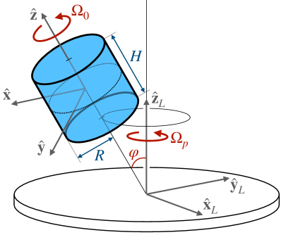
Figure 1: Schematic representation of a fluid-filled precessing cylinder, with radius $R$ and height $H$. The cylinder rotates at angular velocity $\Omega_{0}$ around $\bm{\hat{z}}$, which itself also precesses at angular velocity $\Omega_{p}$ around the vertical axis $\bm{\hat{z}}_{L}$ in the laboratory frame. The precession angle between these two axes is $\varphi$.

To make the problem dimensionless, we use $R$, $\rho$ and $\Omega=\Omega_{0}+\Omega_{p}\cos\varphi$ as characteristic dimensions of length, density and frequency. The problem is associated to four dimensionless numbers: (1) the aspect ratio, $h=H/R$; (2) the forcing frequency, $\omega=\Omega_{0}/\Omega$; (3) the forcing amplitude, $\varepsilon=\Omega_{p}\sin\varphi/\Omega$; and (4) the Ekman number, $\mbox{{Ek}}=\nu/\Omega^{2}R$. Dimensionless quantities will now be noted with lowercase letters. The dimensionless flow velocity in the cylinder framework $(O,\,\bm{\hat{x}},\,\bm{\hat{y}},\,\bm{\hat{z}})$ is denoted by $\bm{u}={\bf{U}}/\left(R\Omega\right)$. We will use the cylindrical coordinates $(r,\theta,z)$, where $z=0$ corresponds to the mid-height of the cylinder and the position vector will be noted $\bf{r}$.

In the cylinder framework, the dimensionless Navier–Stokes equations are (Meunier et al., 2008; Lagrange et al., 2011)

$$\frac{\partial\bm{u}}{\partial t}+2\bm{\hat{z}}\times\bm{u}+\bm{\nabla}p=-2\varepsilon\,\omega r\,\cos(\omega t+\theta)\,\bm{\hat{z}}-2\varepsilon\,\bm{\delta}\times\bm{u}-\bm{u}\cdot\bm{\nabla}\bm{u}+\mbox{{Ek}}\,\bm{\nabla}^{2}\bm{u},$$ (1a)

$$\bm{\nabla}\cdot\bm{u}=0,$$ (1b)

with $\bm{\delta}=\cos(\omega t)\,\bm{\hat{x}}-\sin(\omega t)\,\bm{\hat{y}}$. On the left hand side of (1a), the first term is inertia, the second term is the Coriolis force and $p$ is a dimensionless pressure field including all potential terms (Meunier et al., 2008). On the right hand side of (1a), the first term is the forcing due to precession, the second term is the equatorial Coriolis force, the third term is the convective nonlinear term, and the last term is the viscous force.

We will now consider the asymptotic limits of small Ekman number Ek and small forcing $\varepsilon$, which is achieved when the tilt angle is small or the Poincaré number $\Omega_{p}/\Omega_{0}$ is small. We will seek a solution of the Navier–Stokes equations expressed as a series in powers of these small quantities Ek and $\varepsilon$.

2.1 Inviscid solution

The base flow $\bm{u}^{\left(0\right)}$ forced by precession can be found by solving the Navier-Stokes equations (1a,b) at first order in $\varepsilon$. Following Lagrange et al. (2016), we only keep the first term on the right hand side of (1). The solution $\bm{u}^{\left(0\right)}$ is then composed of two parts: a particular solution in the form of a horizontal shear flow and a sum of Kelvin modes of azimuthal wavenumber $m=1$, which are the solutions of the homogeneous equation. Thus

$$\bm{u}^{\left(0\right)}=\varepsilon\left(\bm{u}_{{\mathrm{shear}}}+\sum\limits_{j=1}^{\infty}A_{j}{\bf v}_{j}\right)\mathrm{e}^{\mathrm{i}\left(\omega t+m\theta\right)}+\mathrm{c.c.},$$ (2)

with $\mathrm{c.c.}$ meaning ‘complex conjugate’. In (2), $\bm{u}_{{\mathrm{shear}}}=\omega z(\mathrm{i}\bm{\hat{r}}-\bm{\hat{\theta}})/(2-\omega)$ is the horizontal shear, $A_{j}$ are the amplitudes of Kelvin modes of axial wavenumber $k_{j}=(2j-1)\pi/h$, and ${\bf v}_{j}$ their associated velocity fields given by

$${\bf v}_{j}=\left(\begin{array}[]{*{20}{r}}\mathrm{i}\,u\,\sin\left(k_{j}z\right)\\ v\,\sin\left(k_{j}z\right)\\ \mathrm{i}\,w\,\cos\left(k_{j}z\right)\\ \end{array}\right),$$ (3)

with $u$, $v$ and $w$, real functions of $r$

$$u(r) =\frac{-1}{4-\omega^{2}}\left(\omega\delta J^{\prime}_{m}\left(\delta r\right)+\frac{2m}{r}J_{m}\left(\delta r\right)\right),$$ (4a)

$$v(r) =\frac{1}{4-\omega^{2}}\left(2\delta J^{\prime}_{m}\left(\delta r\right)+\frac{\omega m}{r}J_{m}\left(\delta r\right)\right),$$ (4b)

$$w(r) =\frac{k}{\omega}J_{m}\left(\delta r\right),$$ (4c)

$J_{m}$ the Bessel function of the first kind, $\delta=k_{j}(4/\omega^{2}-1)^{1/2}$ playing the role of a radial wavenumber, and primes noting differentiation.

Here, we will assume that the forcing is resonant. This occurs when the forcing frequency takes particular values, $\omega=\omega_{n,j}$, such that $u(1)=0$ for a particular Kelvin mode. In that case, this Kelvin mode amplitude $A_{j}$ is asymptotically large and the radial wavenumber takes the value $\delta=\delta_{n,j}=k_{j}(4/\omega_{n,j}^{2}-1)^{1/2}$. Each resonance is associated to a couple of strictly positive integers $(n,j)$: $n$ numbers the radial wavenumber $\delta$ (the function $u(r)$ has exactly $n$ zeros for $0<r\leq 1$), and $j$ numbers the axial wavenumber $k_{j}$ such that $k_{j}=(2j-1)\pi/h$. In Meunier et al. (2008), we also referred to these resonances by the phrase “$j$-th resonance of the $n$-th Kelvin mode”.

At resonance, the amplitude $A_{j}$ of the resonant Kelvin mode can be calculated by either invoking viscous effects, in which case $A_{j}=O(\mbox{{Ek}}^{-1/2})$, or by invoking nonlinear effects, in which case $A_{j}=O(\varepsilon^{-2/3})$ (Meunier et al., 2008). In either case, the base flow is dominated by this single resonant Kelvin mode of amplitude $A=A_{j}$

$$\bm{u}^{\left(0\right)}\approx A\,{\bf v}\,\mathrm{e}^{\mathrm{i}\left(\omega t+m\theta\right)}+\mathrm{c.c.},$$ (5)

whose velocity field ${\bf v}$ is given by (3) and we have dropped the indices $j$ for simplicity.

2.2 Viscous solution

The base flow given in (5) is a solution of the inviscid problem. To satisfy the viscous boundary condition on the walls, it has to be complemented by a boundary-layer solution confined in the wall regions of thickness $O(\mbox{{Ek}}^{1/2})$. The total flow at leading order is then

$$\bm{u}^{(0)}_{\mathrm{tot.}}=A\left({\bf v}+\tilde{{\bf v}}\right)\mathrm{e}^{\mathrm{i}\left(\omega t+m\theta\right)}+\mathrm{c.c.}.$$ (6)

The viscous solution $\tilde{{\bf v}}$ can be expressed as a series in powers of $\mbox{{Ek}}^{1/2}$. This viscous solution has a non-zero axial component $\tilde{w}$ on the end walls at order $\mbox{{Ek}}^{1/2}$, forced through Ekman pumping (Meunier et al., 2008)

$$\tilde{w}(z=-h/2)=\mbox{{Ek}}^{1/2}k^{2}\frac{\mathrm{i}-1}{2\sqrt{2}\,\omega^{2}}\left(\frac{2+\omega}{(2-\omega)^{1/2}}+\mathrm{i}\frac{2-\omega}{(2+\omega)^{1/2}}\right)J_{m}(\delta r)\sin(kh/2),$$ (7)

with an opposite flow on the upper wall in $z=h/2$.

To balance these non-zero axial flows on the end walls, the inviscid solution has to be corrected at order $\mbox{{Ek}}^{1/2}$. A simple way to achieve this correction is to write the axial wavenumber as a series in powers of $\mbox{{Ek}}^{1/2}$

$$k=k^{(0)}+\mbox{{Ek}}^{1/2}k^{(1)}+\cdots,\quad\mbox{with }k^{(0)}=(2j-1)\pi/h,$$ (8)

and

$$k^{(1)}=\frac{k^{(0)}}{\sqrt{2}\,\omega h}(1+\mathrm{i})\left(\frac{2+\omega}{(2-\omega)^{1/2}}+\mathrm{i}\frac{2-\omega}{(2+\omega)^{1/2}}\right).$$ (9)

A similar correction exists for the radial wavenumber $\delta$ since it is proportional to $k$. When there is no ambiguity, we will refer to $k^{(0)}$ as $k$ in the following.

3 Geostrophic flow

The geostrophic flow ${\bf v}_{0}$ is an axisymmetric and steady solution of the linearised Navier–Stokes equation. It thus satisfies the homogeneous equations

$$2\,\bm{\hat{z}}\times{\bf v}_{0}+\bm{\nabla}p_{0}=0,\quad\bm{\nabla}\cdot{\bf v}_{0}=0,$$ (10)

whose solution is

$${\bf v}_{0}=A_{0}v_{0}(r)\,\bm{\hat{\theta}},$$ (11)

where $v_{0}(r)$ can be any function satisfying $v_{0}(0)=0$. Note that the general solution could also include an axial flow $w_{0}(r)$ independent of $z$, which is zero in our case because of the boundary conditions on the end walls.

Similarly to Kelvin modes, this solution of the inviscid problem has to be complemented by a boundary-layer solution in the regions close to the end walls. In these regions of thickness $O(\mbox{{Ek}}^{1/2})$, the total flow is given by

$$\bm{u}_{0}={\bf v}_{0}(r,z)+\tilde{{\bf v}}_{0}(r,\tilde{z})+\mathrm{c.c.},\quad\mbox{with }\tilde{z}=\mbox{{Ek}}^{-1/2}\left(z+\frac{h}{2}\right),$$ (12)

for the lower wall.

Using this rescaled variable $\tilde{z}$ and solving the linearised Navier–Stokes equation with the proper boundary conditions ($\tilde{{\bf v}}_{0}=-{\bf v}_{0}(z=-h/2)$ for $\tilde{z}=0$ and $\tilde{{\bf v}}_{0}\to 0$ for $\tilde{z}\to\infty$), one can write the solution as a series in powers of $\mbox{{Ek}}^{1/2}$

$$\tilde{{\bf v}}_{0}=\tilde{{\bf v}}_{0}^{(0)}+\mbox{{Ek}}^{1/2}\tilde{{\bf v}}_{0}^{(1)}+\cdots,$$ (13)

the leading order solution is

$$\tilde{{\bf v}}_{0}^{(0)}(r,\tilde{z})=-\frac{A_{0}}{2}v_{0}(r)\left(\begin{array}[]{c}\mathrm{i}\mathrm{e}^{-(1+\mathrm{i})\tilde{z}}-\mathrm{i}\mathrm{e}^{-(1-\mathrm{i})\tilde{z}}\\ \mathrm{e}^{-(1+\mathrm{i})\tilde{z}}+\mathrm{e}^{-(1-\mathrm{i})\tilde{z}}\\ 0\\ \end{array}\right).$$ (14)

At next order, an axial flow is forced by Ekman pumping

$$\tilde{w}_{0}^{(1)}(r,\tilde{z})=-\frac{A_{0}}{2r}\frac{\mathrm{d}\left(rv_{0}\right)}{\mathrm{d}r}\left(\frac{1}{(1-\mathrm{i})}\mathrm{e}^{-(1+\mathrm{i})\tilde{z}}+\frac{1}{(1+\mathrm{i})}\mathrm{e}^{-(1-\mathrm{i})\tilde{z}}\right),$$ (15)

which means that there is an inflow of order $O(\mbox{{Ek}}^{1/2}v_{0})$ on the lower wall of velocity

$$\tilde{w}_{0}(z=-h/2)=-\mbox{{Ek}}^{1/2}\frac{A_{0}}{2r}\frac{\mathrm{d}\left(rv_{0}\right)}{\mathrm{d}r},$$ (16)

and, by symmetry, there is the opposite flow on the upper wall.

The important point here is that the inviscid geostrophic flow ${\bf v}_{0}$ is not directly forced, since (10) is homogeneous. But the geostrophic mode can be indirectly forced by symmetric inflows on the cylinder end walls (i.e. $w(z=h/2)=-w(z=-h/2)$). As we shall see in the next section, non-zero symmetric inflows can be created by the precession and the forced Kelvin mode. To cancel these inflows, opposite inflows of the form $\tilde{w}_{0}$ are needed such that $\tilde{w}_{0}(z=-h/2)=-w(z=-h/2)$. It means that a geostrophic flow ${\bf v}_{0}$ can be forced at an order $\mbox{{Ek}}^{-1/2}$ higher than the non-zero inflow $w(z=h/2)$ through (16).

We will now see how non-zero symmetric inflows can be created in precessing flows by four different mechanisms.

4 Forcing of the geostrophic flow

4.1 Interaction between equatorial Coriolis force and the Kelvin mode

The first type of flow that forces a geostrophic flow is ${\bf v}_{k}$, the axisymmetric and steady solution of the linearised Navier–Stokes equation forced by the equatorial Coriolis force, i.e. the second term on the right-hand side of (1). It thus satisfies the following equations

$$2\,\bm{\hat{z}}\times{\bf v}_{k}+\bm{\nabla}p_{k}=\mathbf{F}_{k},\quad\bm{\nabla}\cdot{\bf v}_{k}=0,\quad\mbox{with }\mathbf{F}_{k}=\varepsilon A\,\bm{d}\times{\bf v},$$ (17)

and $\bm{d}=-\bm{\hat{r}}+\mathrm{i}\,\bm{\hat{\theta}}$. A particular solution of this forced equation gives an axial component of velocity

$$w_{k}=-\mathrm{i}\,\varepsilon A\,\frac{1}{2kr}\frac{\mathrm{d}(rw)}{\mathrm{d}r}\sin(kz).$$ (18)

In order to cancel the resulting inflow on the end walls, a geostrophic flow is necessary such that its viscous part satisfies $\tilde{w}_{0}=-w_{k}$ on the lower wall. Using (16), it then leads to a geostrophic flow of order $\mbox{{Ek}}^{-1/2}$ higher than ${\bf v}_{k}$ itself, with azimuthal velocity

$$\left(\bm{u}_{0}\right)_{k}=-\varepsilon\mbox{{Ek}}^{-1/2}\mbox{Im}(A)\frac{2w}{k}\sin(kh/2)\,\bm{\hat{\theta}},$$ (19)

with $\sin(kh/2)=(-1)^{j-1}$, because $k=(2j-1)\pi/h$. Note that velocities noted with the bold letter ‘u’, like $\left(\bm{u}_{0}\right)_{k}$, refer to the real component of the flow and include the complex conjugate, contrarily to velocities denoted by a bold ‘v’, like ${\bf v}_{k}$ for instance.

4.2 Interaction between the Kelvin mode and the shear flow

The second flow that forces a geostrophic flow is ${\bf v}_{\mathrm{shear}}$, the flow forced by the nonlinear interaction of the Kelvin mode with the shear flow. This flow is a solution of

$$2\,\bm{\hat{z}}\times{\bf v}_{\mathrm{shear}}+\bm{\nabla}p_{\mathrm{shear}}=\mathbf{F}_{\mathrm{shear}},\quad\bm{\nabla}\cdot{\bf v}_{\mathrm{shear}}=0,$$ (20)

with

$$\mathbf{F}_{\mathrm{shear}}=-\varepsilon(A\,\overline{\bm{u}}_{\mathrm{shear}}\cdot\bm{\nabla}{\bf v}+\bar{A}\,\overline{{\bf v}}\cdot\bm{\nabla}{\bm{u}}_{\mathrm{shear}}).$$ (21)

The component $\mathbf{F}_{\mathrm{shear}}\cdot\bm{\hat{\theta}}$ has a non-zero real part, which yields through the incompressibility condition to a non-zero axial component of ${\bf v}_{\mathrm{shear}}$

$$w_{\mathrm{shear}}=\varepsilon\,\mbox{Im}(A)\,\frac{1}{2kr}\frac{\partial(rq_{\mathrm{shear}})}{\partial r},$$ (22)

with

$$q_{\mathrm{shear}}=-w(r)\sin(kz)+w(r)\frac{2\delta\omega z}{(2-\omega)\sqrt{4-\omega^{2}}}\cos(kz).$$ (23)

At the end walls $z=\pm h/2$, this axial flow balances exactly the axial flow $w_{k}$ given by (18). It means that a geostrophic flow is created that cancels $\left(\bm{u}_{0}\right)_{k}$

$$\left(\bm{u}_{0}\right)_{\mathrm{shear}}=-\left(\bm{u}_{0}\right)_{k},$$ (24)

with $\left(\bm{u}_{0}\right)_{k}$ given by (19).

4.3 Interaction of the Kelvin mode with itself in the bulk

The third flow that forces a geostrophic flow is the mode ${\bf v}_{2k}$, the axisymmetric and steady solution of the linearised Navier–Stokes equation forced by the nonlinear interactions of the Kelvin mode with itself, which satisfies

$$2\,\bm{\hat{z}}\times{\bf v}_{2k}+\bm{\nabla}p_{2k}=\mathbf{F}_{2k},\quad\bm{\nabla}\cdot{\bf v}_{2k}=0,\quad\mbox{with }\mathbf{F}_{2k}=-|A|^{2}\,\overline{{\bf v}}\cdot\bm{\nabla}{\bf v}.$$ (25)

Note that the radial and axial components of the forcing are much larger than the azimuthal component, which vanishes for an inviscid Kelvin mode. The azimuthal component $\mathbf{F}_{2k}\cdot\bm{\hat{\theta}}$ is $O(|A|^{2}\mbox{{Ek}}^{1/2})$ because of the viscous correction of the Kelvin mode given in (8). This azimuthal component of the forcing is treated below in §4.3.2 through the component $\left(\bm{u}_{0}\right)_{\mathit{Ek}}$ of the geostrophic flow. We will first examine the geostrophic flow due to the radial and axial forcing.

4.3.1 Forcing at order $|A|^{2}$

At leading order $|A|^{2}$, a particular solution of (25) has been given by Waleffe (1989)

$${\bf v}_{2k}=-|A|^{2}v_{2k}(r)\cos(kh)\cos\left(2kz\right)\bm{\hat{\theta}},\quad\mbox{with }v_{2k}(r)=\frac{k}{\omega}\left(\frac{1}{2k}\frac{\mathrm{d}(uv)}{\mathrm{d}r}-vw\right),$$ (26)

with $u$, $v$ and $w$ the radial functions of the Kelvin mode, given in (4).

The velocity ${\bf v}_{2k}$ is solution of the inviscid problem. Although this solution seems to violate the statement of Greenspan (1969) that no geostrophic flow can be generated by an inviscid inertial mode, in fact it does not, since ${\bf v}_{2k}$ is a non-geostrophic zonal flow (because of its dependence on $z$). The associated boundary layer solution can be found by the same method as the one described above for the geostrophic flow in §3. It yields an inflow on the lower wall that can be written

$$\tilde{w}_{2k}(z=-h/2)=|A|^{2}\mbox{{Ek}}^{1/2}\frac{1}{2r}\frac{\mathrm{d}\left(rv_{2k}\right)}{\mathrm{d}r}.$$ (27)

To cancel this inflow, a geostrophic flow is necessary that will produce the opposite flow. This geostrophic flow is found using (16) and can be written

$$\left(\bm{u}_{0}\right)_{2k}=2\,|A|^{2}v_{2k}(r)\,\bm{\hat{\theta}},$$ (28)

Note that the sum of the flow ${\bf v}_{2k}$ and the above geostrophic flow gives a real component of the velocity

$$\bm{u}_{2k}+\left(\bm{u}_{0}\right)_{2k}=2\,|A|^{2}v_{2k}(r)\left(1-\cos(kh)\cos\left(2kz\right)\right)\,\bm{\hat{\theta}},$$ (29)

that cancels for $z=\pm h/2$.

4.3.2 Forcing at order $|A|^{2}\mbox{{Ek}}^{1/2}$

At order $|A|^{2}\mbox{{Ek}}^{1/2}$, the inviscid Kelvin mode interacts nonlinearly with its viscous correction, which can be obtained by a series expansion of $k$ in powers of $\mbox{{Ek}}^{1/2}$ given in (9). This nonlinear interaction can also be viewed as the interaction between the Kelvin mode and the flow resulting from Ekman pumping at the end walls. It yields a non-zero azimuthal forcing $\mathbf{F}_{2k}\cdot\bm{\hat{\theta}}=O(|A|^{2}\mbox{{Ek}}^{1/2})$.

Through (25), this forcing gives rise to a radial velocity $u_{\mathit{Ek}}=\frac{1}{2}\mathbf{F}_{2k}\cdot\bm{\hat{\theta}}$. This radial component induces an axial flow $w_{\mathit{Ek}}$ through the incompressibility condition

$$w_{\mathit{Ek}}(z=-h/2)=|A|^{2}\mbox{{Ek}}^{1/2}\frac{1}{2r}\frac{\mathrm{d}\left(rv_{\mathit{Ek}}\right)}{\mathrm{d}r},\quad\mbox{with }v_{\mathit{Ek}}(r)=\frac{h}{\omega}uw\,\mbox{Im}\left(k^{(1)}\right),$$ (30)

where $k^{(1)}$ is the correction to the axial wavenumber given in (9) and $v_{\mathit{Ek}}$ is found by integrating $\mathbf{F}_{2k}\cdot\bm{\hat{\theta}}$ between $z=-h/2$ and 0 (see also (44) below).

To cancel this flow, a geostrophic flow $\left(\bm{u}_{0}\right)_{\mathit{Ek}}$ is necessary

$$\left(\bm{u}_{0}\right)_{\mathit{Ek}}=2|A|^{2}v_{\mathit{Ek}}(r)\,\bm{\hat{\theta}}.$$ (31)

4.4 Interactions of the Kelvin mode with itself in the boundary layers

Last, we consider the flow $\tilde{{\bf v}}_{\mathit{BL}}$ forced in the end wall boundary layers through nonlinear interactions of the viscous Kelvin mode with itself. Without loss of generality, we consider the lower wall boundary layer of thickness $O(\mbox{{Ek}}^{1/2})$. In this boundary layer, at leading order, the total flow ${\bf v}^{(0)}_{\mathrm{tot.}}$ can be written as the sum of the inviscid solution and its viscous correction

$${\bf v}^{(0)}_{\mathrm{tot.}}=A\sin\left(-kh/2\right)\left(\begin{array}[]{c}\mathrm{i}\,u_{\mathrm{tot.}}\\ v_{\mathrm{tot.}}\\ \mbox{{Ek}}^{1/2}\mathrm{i}\,w_{\mathrm{tot.}}\\ \end{array}\right)\mathrm{e}^{\mathrm{i}\left(\omega t+m\theta\right)},$$ (32)

where $u_{\mathrm{tot.}}$, $v_{\mathrm{tot.}}$ and $w_{\mathrm{tot.}}$ are functions of $r$ and $\tilde{z}$, the rescaled vertical coordinate given by (12). These functions are given by (51a–c) in Appendix A.

Through nonlinear interaction with itself, this flow acts as a steady and axisymmetric forcing of the linearised Navier–Stokes equations

$$\mbox{{Ek}}^{-1/2}\frac{\partial\tilde{p}_{\mathit{BL}}}{\partial\tilde{z}}\bm{\hat{z}}+2\,\bm{\hat{z}}\times\tilde{{\bf v}}_{\mathit{BL}}+\frac{\partial\tilde{p}_{\mathit{BL}}}{\partial r}\bm{\hat{r}}-\frac{\partial^{2}\tilde{{\bf v}}_{\mathit{BL}}}{\partial\tilde{z}^{2}} =\mathbf{F}_{\mathit{BL}},$$ (33a)

$$\mbox{{Ek}}^{-1/2}\frac{\partial\tilde{w}_{\mathit{BL}}}{\partial\tilde{z}}+\frac{1}{r}\frac{\partial\left(r\tilde{u}_{\mathit{BL}}\right)}{\partial r} =0.$$ (33b)

where the forcing term can be written as

$$\mathbf{F}_{\mathit{BL}}(r,\tilde{z})=-{\overline{\bf v}}^{(0)}_{\mathrm{tot.}}\cdot\bm{\nabla}{\bf v}^{(0)}_{\mathrm{tot.}}=|A|^{2}\sum_{i}\left(\begin{array}[]{c}a_{i}+c_{i}\tilde{z}\\ \mathrm{i}b_{i}+\mathrm{i}d_{i}\tilde{z}\\ O(\mbox{{Ek}}^{1/2})\end{array}\right)\mathrm{e}^{-\kappa_{i}\tilde{z}},$$ (34)

with the scalars $\kappa_{i}$ and the functions of $r$, $a_{i}$, $b_{i}$, $c_{i}$, and $d_{i}$, are given in Appendix A.

Equations (33a–b) can be solved by expanding $\tilde{{\bf v}}_{\mathit{BL}}$ in a series of powers of $\mbox{{Ek}}^{1/2}$ and using the boundary conditions, $\tilde{{\bf v}}_{\mathit{BL}}=0$ for $\tilde{z}=0$ and $\tilde{z}\to\infty$. The solution at relevant order is given by (57) in Appendix A. This solution implies a non-zero axial flow $\tilde{w}_{\mathit{BL}}$ at order $|A|^{2}\mbox{{Ek}}^{1/2}$ on the lower end wall. To cancel this inflow, a geostrophic flow is necessary at order $|A|^{2}$ such that

$$\left(\bm{u}_{0}\right)_{\mathit{BL}}=2|A|^{2}v_{\mathit{BL}}(r)\,\bm{\hat{\theta}},$$ (35)

with

$$v_{\mathit{BL}}(r)=\mbox{Re}\left[\sum_{i}\frac{a_{i}\kappa_{i}+\mathrm{i}b_{i}(\kappa_{i}+2))}{\kappa_{i}(\kappa_{i}(\kappa_{i}+2)+2)}+2\frac{c_{i}(\kappa_{i}+1)\kappa_{i}^{2}+\mathrm{i}d_{i}(\kappa_{i}(\kappa_{i}+2)^{2}+2)}{\kappa_{i}^{2}(\kappa_{i}(\kappa_{i}+2)+2)^{2}}\right].$$ (36)

4.5 Total geostrophic flow

We now have calculated the 5 components of the geostrophic flows originating from 5 different inflows at the end walls. These components of the geostrophic flow, noted $\left(\bm{u}_{0}\right)_{k}$, $\left(\bm{u}_{0}\right)_{\mathrm{shear}}$, $\left(\bm{u}_{0}\right)_{2k}$, $\left(\bm{u}_{0}\right)_{\mathit{Ek}}$ and $\left(\bm{u}_{0}\right)_{\mathit{BL}}$, are given respectively by (19), (24),(28), (31) and (35). Summing them up gives the total forced geostrophic flow

$$\bm{u}_{0}=\left(\bm{u}_{0}\right)_{k}+\left(\bm{u}_{0}\right)_{\mathrm{shear}}+\left(\bm{u}_{0}\right)_{2k}+\left(\bm{u}_{0}\right)_{\mathit{Ek}}+\left(\bm{u}_{0}\right)_{\mathit{BL}}=A_{0}v_{0}(r)\,\bm{\hat{\theta}},$$ (37)

with

$$A_{0}=|A|^{2},\quad v_{0}(r)=2v_{2k}(r)+2v_{\mathit{Ek}}(r)+2v_{\mathit{BL}}(r),$$ (38)

and $v_{2k}$, $v_{\mathit{Ek}}$ and $v_{\mathit{BL}}$ given by (26), (30) and (36).

Note that the components $\left(\bm{u}_{0}\right)_{k}$ and $\left(\bm{u}_{0}\right)_{\mathrm{shear}}$ exactly cancel each other, such that the amplitude of the geostrophic flow is proportional to $|A|^{2}$ and does not include any terms proportional to $\varepsilon A\mbox{{Ek}}^{-1/2}$. Because these two terms balance exactly, the resulting geostrophic flow does not depend on the precessional forcing anymore. The present results are thus applicable to any Kelvin mode, independently of the way it has been forced. In particular, as we shall see below, our calculations of the geostrophic flow is valid for Kelvin modes of arbitrary azimuthal wavenumber $m$.

4.6 Weakly non-linear amplitude equations

So far, we have calculated the amplitude of the geostrophic flow $A_{0}$ in the steady regime, and we have found $A_{0}=|A|^{2}$. Based on this calculation and following the weakly nonlinear calculation in Meunier et al. (2008), we can easily obtain the weakly non-linear amplitude equations describing transient regimes.

To obtain the dynamic equations for $A$ and $A_{0}$, we have to correct the term describing non-linear interaction between the geostrophic flow and the Kelvin mode. In Meunier et al. (2008), we did not take into account the components $\left(\bm{u}_{0}\right)_{2k}$ and $\left(\bm{u}_{0}\right)_{\mathit{Ek}}$ of the geostrophic flow and there was also an error in the calculation of $\left(\bm{u}_{0}\right)_{\mathit{Ek}}$ (in particular, the term $w_{4}\tilde{z}$ appearing in (51c) was missing). At resonance, the dynamic amplitude equations are then given by

$$\frac{\mathrm{d}A}{\mathrm{d}t} =\varepsilon\,\mathrm{i}f-\left(\mbox{{Ek}}^{1/2}\mu+\mbox{{Ek}}\,\nu\right)A+\mathrm{i}\left(\sigma|A|^{2}+\xi A_{0}\right)A,$$ (39a)

$$\frac{\mathrm{d}A_{0}}{\mathrm{d}t} =\mbox{{Ek}}^{1/2}\frac{2}{h}\left(|A|^{2}-A_{0}\right),$$ (39b)

where the first 4 coefficients, $f$, $\mu$, $\nu$ and $\sigma$, can be calculated from Meunier et al. (2008) and are given in Table 1 for different resonances. The coefficient $f$ corresponds to the forcing by precession while $\mu$ and $\nu$ correspond to the Ekman and volume damping. The coefficient $\sigma$ corresponds to the non-linear coupling of the Kelvin mode with the non-geostrophic flow ${\bf v}_{2k}$ and with an unsteady elliptic flow noted ${\bf v}_{2\omega}$ in Meunier et al. (2008).

The weakly nonlinear coefficient $\xi$, accounting for the nonlinear coupling between the Kelvin mode and the geostrophic flow, can be calculated as follows. We first calculate the nonlinear interaction of the Kelvin mode with the geostrophic flow: $\bm{u}_{0}\cdot\nabla{\bf v}+{\bf v}\cdot\nabla\bm{u}_{0}$. We then project this forcing onto the Kelvin mode using the natural Hermitian product over the cylinder volume. The coefficient $\xi$ is simply this Hermitian product normalised by the norm of the Kelvin mode (which is nothing else than its kinetic energy). It can be written $\xi=X/E$ with

$$X=2\pi h|A|^{2}\int_{0}^{1}\left(\frac{2k}{\omega}uw\,v_{0}-uv\frac{1}{r}\frac{\mathrm{d}(rv_{0})}{\mathrm{d}r}\right)r\,\mathrm{d}r,$$ (40)

$E$ the kinetic energy of the mode

$$E=2\pi h|A|^{2}\frac{2k^{2}+m(2m-\omega)}{(4-\omega^{2})\,\omega^{2}}J_{m}(\delta)^{2},$$ (41)

and $v_{0}(r)$ given by (38). The values of $\xi$ for the first nine resonances are plotted in figure 2. It shows that $\xi$ scales as $-h^{-4}$ for $h\ll 1$, changes sign for $h=O(1)$ and scales as $h$ for $h\gg 1$.

Table 1: Coefficients appearing in the weakly nonlinear amplitude equations (39) for different resonances $(n,j)$ and different aspect ratios $h$.

$(n,j)$	$h$	$\omega_{n,j}$	$f$	$\mu$	$\nu$	$\sigma$	$\xi$
$(1,1)$	$1.62$	$1.181$	$0.452$	$1.86-0.42\mathrm{i}$	$10.78$	$0.13$	$-2.94$
$(1,1)$	$1.8$	$1.088$	$0.467$	$1.80-0.27\mathrm{i}$	$10.29$	$-0.06$	$-2.31$
$(1,1)$	$2$	$0.996$	$0.469$	$1.73-0.13\mathrm{i}$	$9.96$	$0.23$	$-1.84$
$(2,1)$	$2$	$0.510$	$-0.074$	$1.58+0.11\mathrm{i}$	$37.99$	$-10.69$	$0.14$
$(3,1)$	$2$	$0.339$	$0.025$	$1.47+0.16\mathrm{i}$	$85.90$	$-59.92$	$43.03$
$(1,2)$	$2$	$1.774$	$-0.042$	$0.84-0.40\mathrm{i}$	$28.24$	$7.80$	$-40.97$
$(2,2)$	$2$	$1.285$	$0.021$	$1.40-0.26\mathrm{i}$	$53.77$	$9.96$	$-53.06$
$(3,2)$	$2$	$0.946$	$-0.009$	$1.52-0.09\mathrm{i}$	$99.28$	$2.54$	$-84.55$
$(1,3)$	$2$	$1.911$	$-0.007$	$0.50-0.32\mathrm{i}$	$67.56$	$50.93$	$-255.44$
$(2,3)$	$2$	$1.632$	$-0.006$	$1.05-0.39\mathrm{i}$	$92.60$	$66.39$	$-225.67$
$(3,3)$	$2$	$1.339$	$0.004$	$1.34-0.28\mathrm{i}$	$137.55$	$61.01$	$-272.52$

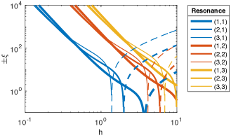
Figure 2: Value of the weakly nonlinear coefficient $\xi$ as a function of the aspect ratio $h$. The value is given for different resonances $(n,j)$ as noted in the legend and we use the convention of a solid line for $\xi$ negative and a dashed line for $\xi$ positive.

This weakly nonlinear analysis will be used below to predict the amplitude $A_{0}$ of the geostrophic flow when nonlinear effects are not negligible.

5 Comparison with numerical results

We first examine the resonance $(n=1,j=1)$, which occurs when the radial velocity $u(r)$ of the resonant Kelvin mode has one zero for $0<r\leq 1$ (this zero being in $r=1$) and when the wavenumber is $k=\pi/h$.

In order to compare our theoretical results with the numerical results of Albrecht et al. (2020), we focus on the aspect ratio $h=1.62$ for which the $(1,1)$ resonance is obtained at a forcing frequency $\omega_{1,1}=1.181$ (table 1). The tilt angle is small, $\varphi=0.4^{\circ}$, and corresponds to a forcing amplitude $\varepsilon=-0.00127$, such that there is no instability in the numerical simulations at $\mbox{{Ek}}=1.538\times 10^{-4}$.

For these parameters, the forced Kelvin mode is mainly saturated by viscous effects and we can neglect nonlinear terms in (39a). The Kelvin mode amplitude is then

$$A=\frac{\varepsilon\mathrm{i}f}{\mbox{{Ek}}^{1/2}\mu+\mbox{{Ek}}\,\nu}$$ (42)

where the coefficients $f$, $\mu$ and $\nu$, given in table 1, correspond to $A=0.0047-0.0221\,\mathrm{i}$. Using this value and (41), the total kinetic energy is found to be $E=0.0025$. This kinetic energy is approximately 30% lower than the kinetic energy found in numerical simulations by isolating the azimuthal wavenumber $m=1$ (Albrecht et al., 2020). Equation (42) thus underestimates the amplitude $A$ by about 14% in this case.

5.1 Spatial structure of the forcing

In the Navier–Stokes equations, the interaction of the forced Kelvin mode with the time-dependent precession forcing gives rise to a forcing term $\mathbf{F}_{k}$ given in (17). This term is noted $\mathcal{C}^{\mathrm{inv}}$ in the paper of Albrecht et al. (2020). The three components of $\mathbf{F}_{k}$ along $\bm{\hat{r}}$, $\bm{\hat{\theta}}$ and $\bm{\hat{z}}$ are plotted in figure 3a–c.

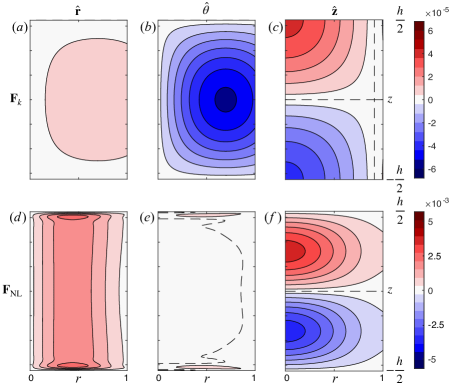
Figure 3: Forcing terms of the different components of the geostrophic flow. The columns are, from left to right, the radial (a, d), azimuthal (b, e), and axial (c, f) components of the forcing terms. The components of the forcing term $\mathbf{F}_{k}$ given in (17) are shown in a–c. The components of the forcing term $\mathbf{F}_{\mathrm{NL}}=\mathbf{F}_{\mathrm{shear}}+\mathbf{F}_{2k}+\mathbf{F}_{\mathit{BL}}$ given in (21), (25) and (34) are shown in d–f. The dashed line shows the level line for zero. The parameters are $h=1.62$, $\mbox{{Ek}}=1.5\times 10^{-4}$, $\omega=1.181$ and $\varepsilon=-0.00127$. To ease the comparison with figure 6 of Albrecht et al. (2020), we use the same contours.

They are in excellent agreement with the numerical results of Albrecht et al. (2020) (see their figures 6d–f). The largest component is the $\theta$-component, which has a unique negative lobe with a minimum value equal to $-5.4\times 10^{-5}$, while in the numerical simulations this value is approximately $-6\times 10^{-5}$ (Albrecht et al., 2020). A small difference between the numerics and the theory is also found for the axial component: the numerical results have a 20% smaller amplitude; they exhibit small undulations of the iso-contours (probably due to inertial waves of small amplitudes emitted from the corners); and, in the simulations, this term vanishes at the top and the bottom because of the viscous boundary layers.

The nonlinear forcing terms can be gathered into a single forcing term $\mathbf{F}_{\mathrm{NL}}=\mathbf{F}_{\mathrm{shear}}+\mathbf{F}_{2k}+\mathbf{F}_{\mathit{BL}}$, which is noted $\mathcal{R}^{\mathrm{inv}}$ in Albrecht et al. (2020). The three components of $\mathbf{F}_{\mathrm{NL}}$ are plotted in figure 3d–f. The forcing $\mathbf{F}_{\mathrm{NL}}$ gathers all nonlinear interactions of the forced flow with itself, including the Kelvin mode at order $A$, but also the particular shear flow solution at a lower order $O(\varepsilon)$, given by (2), and the viscous correction to the Kelvin mode, also at a lower order $O(A\mbox{{Ek}}^{1/2})$, obtained by a series expansion of the wavenumber $k$ given in (9). Figure 3d–f shows an excellent agreement with the numerical results of Albrecht et al. (2020) plotted in their figures 6g–i. The largest component of $\mathbf{F}_{\mathrm{NL}}$ is the axial component and it exhibits a negative and a positive lobe with a maximum value of $3.6\times 10^{-3}$, while it is of $5\times 10^{-3}$ in the simulations. The radial component has a weak dependence on $z$ and the azimuthal component is of order $Ek^{1/2}$ weaker than the other components, except for $\mathbf{F}_{\mathit{BL}}$ in the boundary layers.

The azimuthal component of the axisymmetric forcing, $F_{\mathrm{az.}}=\mathbf{F}\cdot\bm{\hat{\theta}}$, plays a particular role here because it induces a geostrophic flow at an order $\mbox{{Ek}}^{-1/2}$ higher than itself. The reason is that $F_{\mathrm{az.}}$ directly forces a radial flow through the $\theta$-projection of the Navier–Stokes equation, $u_{\mathrm{az.}}=\frac{1}{2}F_{\mathrm{az.}}$, which itself forces an axial flow through the incompressibility condition

$$w_{\mathrm{az.}}(r,z)=-\int\frac{1}{r}\frac{\partial(ru_{\mathrm{az.}})}{\partial r}\,\mathrm{d}z.$$ (43)

To cancel the $z$-odd part of this flow on the end walls, a geostrophic flow is necessary such that $(\tilde{w}_{0})_{\mathrm{az.}}=-w_{\mathrm{az.}}$ in $z=-h/2$. This axial flow then yields a geostrophic flow

$$(v_{0})_{\mathrm{az.}}(r)=\mbox{{Ek}}^{-1/2}\int_{-h/2}^{0}F_{\mathrm{az.}}\,\mathrm{d}z.$$ (44)

The $\theta$-component of the axisymmetric forcing $F_{\mathrm{az.}}$ therefore induces a geostrophic flow at order $F_{\mathrm{az.}}\mbox{{Ek}}^{-1/2}$, which is found to be proportional to the $z$-average of $F_{\mathrm{az.}}$. Here, we note that this reasoning allows us to show that the non-linear interactions between two Kelvin modes of different axial wavenumbers do not force a geostrophic flow. For instance, consider a non-resonant Kelvin mode of real amplitude $A_{i}=O(\varepsilon)$ and wavenumber $k_{i}=(2i-1)\pi/h$ interacting with the resonant Kelvin mode of amplitude $A$ and wavenumber $k=(2j-1)\pi/h$. The non-linear interactions will yield a non-zero azimuthal forcing $F_{\mathrm{az.}}$ with terms proportional to $\varepsilon\,\mbox{Im}(A)\cos(k\pm k_{i})z$. However, using (44), we see that this forcing does not give rise to any geostrophic flow because the sum or difference of axial wavenumbers, $(k\pm k_{i})$, will always be an integer multiple of $2\pi/h$ and will have a zero average along $z$.

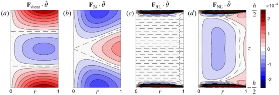
Figure 4: Azimuthal forcing terms of the different components of the geostrophic flow: (a) $\mathbf{F}_{\mathrm{shear}}\cdot\bm{\hat{\theta}}$; (b) $\mathbf{F}_{2k}\cdot\bm{\hat{\theta}}$; (c) $\mathbf{F}_{\mathit{BL}}\cdot\bm{\hat{\theta}}$; (d) $\mathbf{F}_{\mathrm{NL}}\cdot\bm{\hat{\theta}}$, with $\mathbf{F}_{\mathrm{NL}}=\mathbf{F}_{\mathrm{shear}}+\mathbf{F}_{2k}+\mathbf{F}_{\mathit{BL}}$. Parameters are the same as in figure 3.

The azimuthal components of the different forcing terms are plotted in figures 3b,e and 4a–d. It shows that $\mathbf{F}_{k}\cdot\bm{\hat{\theta}}$ and $\mathbf{F}_{\mathrm{NL}}\cdot\bm{\hat{\theta}}$ are both negative (except near $r=1$ for $\mathbf{F}_{\mathrm{NL}}\cdot\bm{\hat{\theta}}$), even if the components $\mathbf{F}_{\mathrm{shear}}\cdot\bm{\hat{\theta}}$ and $\mathbf{F}_{\mathit{BL}}\cdot\bm{\hat{\theta}}$ have positive average along $z$.

5.2 Zonal flow

The geostrophic flow $\left(\bm{u}_{0}\right)_{k}$ produced in response to $\mathbf{F}_{k}$ is plotted in figure 5a. Its azimuthal velocity is always negative with a minimum value equal to $-2.2\times 10^{-3}$ in good agreement with the minimum value of about $-2.5\times 10^{-3}$ found numerically by Albrecht et al. (2020) (see their figure 6o). However, in the numerical simulations, the azimuthal velocity vanishes at $r=1$ in order to satisfy the no-slip boundary conditions whereas it remains negative in the present theory.

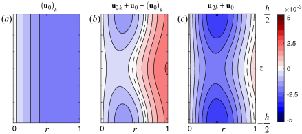
Figure 5: Mean azimuthal flow generated by different sources. (a) Velocity $\left(\bm{u}_{0}\right)_{k}$ given by (19) and induced by the forcing $\mathbf{F}_{k}$. (b) Velocity $\left(\bm{u}_{0}\right)_{\mathrm{shear}}+\bm{u}_{2k}+\left(\bm{u}_{0}\right)_{2k}+\left(\bm{u}_{0}\right)_{\mathit{Ek}}+\left(\bm{u}_{0}\right)_{\mathit{BL}}=\bm{u}_{2k}+\bm{u}_{0}-\left(\bm{u}_{0}\right)_{k}$ given by (24), (29), (30) and (35) and induced by the nonlinear forcing term $\mathbf{F}_{\mathrm{NL}}$. (c) Total azimuthal velocity $\bm{u}_{2k}+\bm{u}_{0}$ induced by all sources. Parameters are the same as in figures 3 and 4.

The azimuthal flow $\left(\bm{u}_{0}\right)_{\mathrm{shear}}+\bm{u}_{2k}+\left(\bm{u}_{0}\right)_{2k}+\left(\bm{u}_{0}\right)_{\mathit{Ek}}+\left(\bm{u}_{0}\right)_{\mathit{BL}}=\bm{u}_{2k}+\bm{u}_{0}-\left(\bm{u}_{0}\right)_{k}$ in response to the nonlinear forcing term $\mathbf{F}_{\mathrm{NL}}$ is plotted in figure 5b. It exhibits two negative lobes of azimuthal velocity with a minimal value equal to $-1.6\times 10^{-3}$. This value can be compared to the value of $-2.5\times 10^{-3}$ found numerically by Albrecht et al. (2020) (their figure 6s), and the difference can be explained by the 30% difference in the Kelvin mode kinetic energy.

Adding all responses yields the zonal flow $\bm{u}_{2k}+\bm{u}_{0}$ (figure 5c). It is almost everywhere negative except near the lateral wall around the equator. The velocity distribution is quantitatively similar to that found numerically by Albrecht et al. (2020) in their figure 6k. We find a minimum value of $-3.3\times 10^{-3}$, close to the numerical value of $-4.5\times 10^{-3}$ with again a difference that can mainly be imputed to the 30% difference in kinetic energy.

Averaging this total flow over the height of the cylinder filters out the non-geostrophic response $\bm{u}_{2k}$ leading to the total geostrophic flow $\bm{u}_{0}$. This geostrophic flow, plotted in figure 6 as a black solid line, is in excellent agreement with the numerical result of Albrecht et al. (2020) plotted as a black dotted line. This geostrophic flow contains several terms, the Coriolis term $\left(\bm{u}_{0}\right)_{k}$ being exactly opposite to the shear term $\left(\bm{u}_{0}\right)_{\mathrm{shear}}$. Apart from these two terms, the dominant contribution comes from the nonlinear coupling between the inviscid Kelvin mode and its viscous correction in the bulk $\left(\bm{u}_{0}\right)_{\mathit{Ek}}$, which is retrograde. This flow is weakly compensated by the geostrophic adaptation $\left(\bm{u}_{0}\right)_{2k}$ to the zonal flow $vit_{2k}$ and by the nonlinear coupling in the boundary layers $\left(\bm{u}_{0}\right)_{\mathit{BL}}$. We note here that $\left(\bm{u}_{0}\right)_{2k}$ and $\left(\bm{u}_{0}\right)_{\mathit{BL}}$ are approximately equal for the parameters chosen. This is merely incidental.

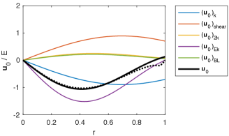
Figure 6: Geostrophic flow generated by different sources. The components $\left(\bm{u}_{0}\right)_{k}$, $\left(\bm{u}_{0}\right)_{\mathrm{shear}}$, $\left(\bm{u}_{0}\right)_{2k}$, $\left(\bm{u}_{0}\right)_{\mathit{Ek}}$ and $\left(\bm{u}_{0}\right)_{\mathit{BL}}$, given by (19), (24), (28), (31) and (35), are represented by solid lines. They sum up to form the total geostrophic flow $\bm{u}_{0}$ (black solid line). The velocity is normalized by the kinetic energy of the Kelvin mode $E$. The dotted black line show the numerical results of Albrecht et al. (2020) for the same parameters (see their figure 10). Parameters are the same as in figures 3 and 5.

5.3 Dependence of the zonal flow on the aspect ratio $h$

We have shown that, in the steady case, the geostrophic flow is proportional to $|A|^{2}$. This was also found numerically by Albrecht et al. (2020): in their figure 11c, they showed that the ratio between the kinetic energy of the azimuthal flow $E_{0}$ and the square of the kinetic energy of the Kelvin mode $E^{2}$ is nearly independent of the Ekman number and the tilt angle. Here, we show that $E_{0}$ is proportional to $|A|^{4}$, while $E$ given by (41) is proportional to $|A|^{2}$, which is consistent with the observation of Albrecht et al. (2020).

Although the ratio $E_{0}/E^{2}$ is independent on the forcing amplitude $\varepsilon$ and Ekman number Ek, it depends on the aspect ratio $h$. This is because the aspect ratio influences the resonant frequency $\omega_{n,j}$ and the radial wavenumber $\delta_{n,j}$. In figure 7, we compare the quantity $E_{0}/E^{2}$ extracted from Albrecht et al. (2020) to our prediction, when $h$ is varied.

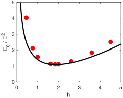
Figure 7: Ratio between the kinetic energy $E_{0}$ of the zonal flow $\bm{u}_{2k}+\bm{u}_{0}$ and the squared kinetic energy $E$ of the forced Kelvin mode. This ratio is plotted as a function of the aspect ratio $h$ for the $(1,1)$ resonance. The symbols correspond to the numerical results obtained by Albrecht et al. (2020) for $\mbox{{Ek}}=2\times 10^{-4}$. The solid line corresponds to the present theory.

The theoretical prediction is found to be in excellent agreement with these numerical results although the theory tends to slightly underestimate the axisymmetric flow in the limit of small and large aspect ratios. This may be due to the presence of the boundary layers on the cylinder side walls.

6 Comparison with experimental results

We shall now compare the present theoretical predictions with the experimental results of Meunier et al. (2008).

We start with the $(1,1)$ resonance. The aspect ratio is $h=1.8$, giving a resonant frequency $\omega_{1,1}=1.088$ (table 1). The tilt angle is $\varphi=2^{\circ}$, which corresponds to a forcing amplitude $\varepsilon=-0.0031$. The mean azimuthal velocity has been measured for three moderate Ekman numbers at $z=h/4$ (figure 8). In each case, the azimuthal velocity is negative meaning that the zonal flow is retrograde.

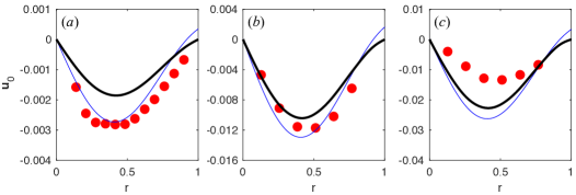
Figure 8: Mean azimuthal velocity profiles of the $(1,1)$ resonance. Symbols are the experimental results of Meunier et al. (2008) measured at $z=h/4$, while the solid lines represent the velocity profiles predicted: $|A|^{2}v_{0}$ given by (38) in blue and $|A|^{2}\left(v_{0}\right)_{\mathrm{vol.}}$ given by (47) in black. Parameters are: $h=1.8$, $\omega=1.088$, $\varepsilon=-0.0031$ and three different Ekman numbers: (a) $\mbox{{Ek}}=8.1\times 10^{-4}$; (b) $\mbox{{Ek}}=2.0\times 10^{-4}$; and (c) $\mbox{{Ek}}=0.81\times 10^{-4}$.

We first compute the amplitudes of the Kelvin mode and geostrophic flow by looking for the fixed point $(A,A_{0})$ of the weakly nonlinear amplitude equations (39). We then plot the resulting geostrophic flow $\bm{u}_{0}$ for two cases: first we consider the profile $v_{0}$ obtained in section 4 and given by (38), second we take into account viscous effects onto the geostrophic flow by proceeding as follows. We decompose $v_{0}(r)$ into Bessel functions of the first kind

$$v_{0}(r)=\sum_{i=1}^{\infty}A_{i}J_{1}(d_{i}r),\quad\mbox{such that }J_{1}(d_{i})=0.$$ (45)

where the amplitudes $A_{i}$ can be calculated as

$$A_{i}=\frac{2}{J_{0}^{2}(d_{i})}\int_{0}^{1}v_{0}(r)J_{1}(d_{i}r)\,r\,\mathrm{d}r.$$ (46)

This decomposition is analogue to a Fourier decomposition. The $d_{i}$’s are the zeros of $J_{1}$ ordered in ascending order. They play the role of radial wavenumbers for the geostrophic flow and satisfy $d_{i}\sim i\pi$ for large $i$.

When the geostrophic flow $v_{0}$ is decomposed as in (45), the viscous term of the Navier–Stokes equations, $\mbox{{Ek}}\,\nabla^{2}\bm{u}_{0}$, gives rise to an azimuthal forcing $F_{\mathrm{az.}}=-\sum_{i}A_{i}d_{i}^{2}J_{1}(d_{i}r)$, which itself yields a geostrophic flow $\mbox{{Ek}}^{1/2}F_{\mathrm{az.}}h/2$ through the reasoning explained above in §5.1. The corrected azimuthal flow taking into account this effect is then given by

$$\left(v_{0}\right)_{\mathrm{vol.}}(r)=\sum_{i=1}^{\infty}\frac{A_{i}}{1+\mbox{{Ek}}^{1/2}d_{i}^{2}h/2}J_{1}(d_{i}r).$$ (47)

This way to incorporate viscous effects has been first introduced in Meunier et al. (2008). It accounts for both the side wall boundary layer and the Ekman pumping from end walls. In the limit of small Ek, we recover at leading order the $O(\mbox{{Ek}}^{1/4})$ side wall boundary layer obtained by Wang (1970) (see appendix B). The $O(Ek^{1/2})$ correction induced by the Ekman pumping in the bulk depends however on the Bessel decomposition (45) of $v_{0}$. This correction is the smallest if the spectral content of $v_{0}$ is mainly on small radial wavenumbers. For the geostrophic flows plotted in figure 8, the smallest wavenumber $d_{1}$ is dominant. Viscous effects are therefore expected to be negligible as soon as the Ekman number is asymptotically small compared to $d_{1}^{-4}h^{-2}\approx 10^{-3}$.

This is the case in figure 8c and in the numerical simulations shown in the previous section, but not for the case of figures 8a. Note that, in the limit $\mbox{{Ek}}\ll d_{1}^{-4}h^{-2}$, the flow is generally unstable unless the tilt angle is extremely small, which is difficult to achieve experimentally.

Comparing the experimental velocity profiles and the theoretical predictions in figure 8 shows a good agreement. Both profiles have the same bell shape with a minimum value reached around $r\approx 0.4$. The amplitude is underpredicted by 30% for the lower Ekman number and overpredicted by a factor almost 2 for the highest value. This latter discrepancy may be due to large nonlinear effects and an instability of the Kelvin mode.

The comparison for the $(2,1)$ resonance is shown in figure 9. In this case, the viscous effects on the geostrophic flow are even more pronounced than for the $(1,1)$ resonance in figure 8. This is because of the importance of the second amplitude $A_{2}$ in the Bessel series (45). The agreement between theory and experiment is excellent both qualitatively and quantitatively. Both profiles are negative with two local minima: the largest one is around $r=0.25$ and the second one around $r=0.75$. The amplitudes predicted by $\left(v_{0}\right)_{\mathrm{vol.}}$ compare well with experimental results for the two largest values of the Ekman number. For the smallest Ekman number, as for the first resonance, the discrepancy may be due to nonlinearities or an instability.

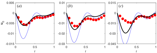
Figure 9: Same as figure 8 for the $(2,1)$ resonance. Parameters are: $h=2$, $\omega=0.510$, $\varepsilon=-0.0086$, $z=h/4$ and (a) $\mbox{{Ek}}=2.66\times 10^{-4}$; (b) $\mbox{{Ek}}=1.33\times 10^{-4}$; and (c) $\mbox{{Ek}}=0.66\times 10^{-4}$.

7 Retrograde sign of the geostrophic flow

So far, we have found that the geostrophic flow is always retrograde. This is a classical observation in precessing flows, where precession tends to slow down the solid body rotation (Kobine, 1996; Meunier et al., 2008). Although this seems intuitive, there is no proof of this result so far. In fact, nothing prevents precession from spinning up the solid body rotation because the precessional motion injects energy in the system. For instance, this is what would happen if only the nonlinear term $(\bm{u}_{0})_{\mathit{BL}}$ was considered for the $(1,1)$ resonance (figure 6).

To assess whether the zonal flow $\bm{u}_{0}+\bm{u}_{2k}$ is always retrograde, we calculate its angular momentum defined as

$$M_{0}=\bm{\hat{z}}\cdot\int_{V}\bm{r}\times\left(\bm{u}_{0}+\bm{u}_{2k}\right)\,\mathrm{d}V=2\pi hA_{0}\int_{0}^{1}r^{2}v_{0}(r)\,\mathrm{d}r,$$ (48)

which in fact only depends on the geostrophic component $\bm{u}_{0}$, the non-geostrophic part $\bm{u}_{2k}$ being periodic along $z$. In figure 10a, we see that this angular momentum (normalized by the kinetic energy of the Kelvin mode $E$) is always negative for the range of aspect ratios and resonances chosen.

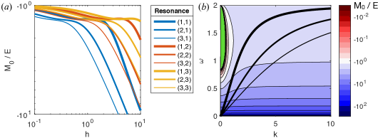
Figure 10: Angular momentum $M_{0}$ of the geostrophic flow normalised by the kinetic energy of the Kelvin mode $E$ for a resonant precessing cylinder ($m=1$). In (a), the angular momentum is plotted as a function of the aspect ratio $h$ for different resonances as mentioned in the legend. In (b), the angular momentum is plotted as contours in the $(k,\omega)$-plane. The green zone corresponds to positive values of the angular momentum, but this zone is not accessible due to the dispersion relation. The black lines show this dispersion relation for the first three resonances: $(1,\cdot)$ thick line; $(2,\cdot)$ medium line; and $(3,\cdot)$ thin line (the higher resonances have lower $\omega$).

The angular momentum $(M_{0})_{\mathit{BL}}$ due to the component $(v_{0})_{\mathit{BL}}$ of the geostrophic flow is complex, but if we first focus on the components $(v_{0})_{2k}$ and $(v_{0})_{\mathit{Ek}}$ of the geostrophic flow, we can show that their associated angular momenta simplify into

$$\frac{\left(M_{0}\right)_{2k}}{E} = 1-m\frac{\omega k^{2}+m(m\omega-2)}{2k^{2}+m(2m-\omega)}.$$ (49)

$$\frac{\left(M_{0}\right)_{\mathit{Ek}}}{E} = -\frac{hm}{k}\,\mbox{Im}\left(k^{(1)}\right)=-\frac{m}{\sqrt{2}\,\omega}\left(\frac{2+\omega}{(2-\omega)^{1/2}}+\frac{2-\omega}{(2+\omega)^{1/2}}\right),$$ (50)

where $E$ is the kinetic energy of the Kelvin mode given by (41). The ratio $(M_{0})_{\mathit{Ek}}/(mE)$ is a function of $\omega$ only that is always negative on the interval $0<\omega<2$. With some calculation, it can also be shown that the sum $(M_{0})_{2k}+(M_{0})_{\mathit{Ek}}$ is always negative for $m\geq 1$, $k>0$ and $0<\omega<2$.

To show numerically that the total angular momentum is always retrograde, we use the fact that the ratio $(M_{0})_{\mathit{BL}}/E$ is a function of $k$ and $\omega$ only. Although this function is too complex to reproduce here, it can be easily plotted. We can thus plot the total angular momentum $M_{0}/E$ in the $(k,\omega)$-plane for $m=1$ (figure 10b). In this plane, we see that the angular momentum is everywhere negative, except in a small region for small $k$ and $0.8\lesssim\omega<2$ (green region in figure 10b). However, this region is not reachable by any resonance, because $k$ and $\omega$ are linked by the dispersion relation $u(1)=0$ with $u$ given in (4a). This dispersion relation is plotted as black lines in figure 10b for the first three resonances. For higher resonances, the angular frequency continue to decrease and moves further aways from the zone of positive angular momentum. It thus shows that the angular momentum is always retrograde for $m=1$ and $0<\omega<2$.

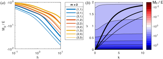
Figure 11: Same as figure 10 for the Kelvin modes of azimuthal wavenumber $m=2$.

Although the calculations presented in this paper focused on Kelvin modes of azimuthal wavenumber $m=1$ forced by precession, they are easily generalisable to different azimuthal wavenumbers. In figure 11, we consider the azimuthal wavenumber $m=2$. It shows again that a resonant Kelvin modes always forces a retrograde geostrophic flow. In this case, it is even simpler because, contrarily to $m=1$, there is no region of positive angular momentum in the $(k,\omega)$-plane.

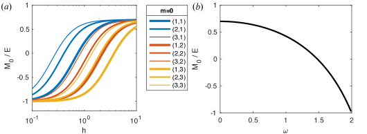
Figure 12: Same as figure 10 for the Kelvin modes of azimuthal wavenumber $m=0$. In this case, the ratio between the angular momentum $M_{0}$ and the kinetic energy $E$ is only a function of $\omega$ represented in (b). It changes sign for $\omega\approx 1.48$.

The situation is different for the azimuthal wavenumber $m=0$ (figure 12). In this case, the sign of the angular momentum $M_{0}$ is positive for $\omega\lesssim 1.48$ and negative for $\omega\gtrsim 1.48$ (figure 12b). It thus means that the geostrophic flow will be retrograde in the limit of small aspect ratio but prograde in the limit of large aspect ratio (figure 12a).

The figures 10b and 11b show numerically that the geostrophic flow is always retrograde for azimuthal wavenumbers $m=1$, $2$ and for forcing frequency in the interval $0<\omega<2$. The situation is similar for $m=3$ (not shown here) and presumably for higher values of the azimuthal wavenumber. But again, this is difficult to prove mathematically given the complexity of $(M_{0})_{\mathit{BL}}$.

Note that for negative forcing frequency ($\omega<0$), the geostrophic flow could be prograde. This corresponds to the particular case of a cylinder rotating around its axis with a frequency $0<\Omega_{0}<-\Omega_{p}$, with $\Omega_{p}<0$ the precession frequency. Usually, experiments and numerical simulations do not consider this limit and rather focus on proper frequencies larger than precession frequencies ($|\Omega_{0}|>|\Omega_{p}|$).

8 Conclusion

In this paper, we have provided an analytic expression of the zonal flow in a precessional cylinder at resonance. In this regime, the harmonic response is dominated by a single Kelvin mode of amplitude $A$, azimuthal wavenumber $m=1$ and axial wavenumber $k$. We have identified five contributions to the zonal flow.

The first contribution, noted $\left(\bm{u}_{0}\right)_{k}$, and given by (19), comes from the interaction of the Kelvin mode with the equatorial Coriolis force. The second contribution comes from the interaction of the Kelvin mode with the axial shear (i.e. the particular solution to the Poincaré forcing). Surprisingly, its expression is exactly opposite to $\left(\bm{u}_{0}\right)_{k}$ whatever the Kelvin mode. As a consequence, these two first contributions, which are specific to the precessing cylinder, cancel each other.

The three other contributions come from the interaction of the Kelvin mode with itself. They are therefore not specific to the precessing cylinder and their expressions have been provided for any $k$ and $m$. The first one corresponds to the steady and axisymmetric term $\bm{u}_{2k}$ of amplitude $|A|^{2}$ and axial wavenumber $2k$, which is forced by the nonlinear interaction of the inviscid Kelvin mode with itself. This inviscid (non-geostrophic) zonal flow exhibits a non-zero azimuthal velocity on the end walls. It must be complemented by a geostrophic flow $\left(\bm{u}_{0}\right)_{2k}$ to satisfy the no-slip boundary condition. The sum of these two terms is given analytically in (29).

The second Kelvin mode source of zonal flow comes from the nonlinear interaction of the inviscid Kelvin mode with its viscous correction in the bulk. This weak forcing of order $|A|^{2}\mbox{{Ek}}^{1/2}$ generates an axial flow of order $|A|^{2}\mbox{{Ek}}^{1/2}$ with non-zero velocity at the end walls. Such a flow must thus be compensated by the Ekman pumping of a geostrophic flow, $\left(\bm{u}_{0}\right)_{\mathit{Ek}}$, of order $|A|^{2}$ given in (31).

Finally, the third Kelvin mode contribution to the zonal flow comes from the nonlinear self-interaction of the flow inside the end wall boundary layers. It generates a non-zero axial flow at the end walls, of order $|A|^{2}\mbox{{Ek}}^{1/2}$, which again must be compensated by a geostrophic flow of order $|A|^{2}$, given analytically in (35).

We have used these expressions to derive the coupled equations that describe the slow dynamics of the Kelvin mode amplitude and the geostrophic flow amplitude. These equations also provide the saturation amplitude of the Kelvin mode. The variation of the nonlinear coefficient coming from the interaction with the zonal flow has been analysed as a function of the cylinder aspect ratio for the first nine resonances.

The present results have been compared to the numerical simulations of Albrecht et al. (2020) and to the experimental measurements of Meunier et al. (2008). A good agreement has been observed, especially when the viscous correction to the zonal flow was considered.

We have also computed the angular momentum of the zonal flow to assess whether it is prograde (positive angular momentum) or retrograde (negative angular momentum). This has allowed us to show numerically that the zonal flow is always retrograde for $m=1$, $2$, or $3$, and presumably for larger $m$.

The zonal flow has been calculated for any Kelvin mode. Our results can thus be applied to other azimuthal forcing, such as libration. This $m=0$ forcing has been studied in a cylinder by Wang (1970); Noir et al. (2010); Busse (2010); Lopez & Marques (2011); Sauret et al. (2012). Wang (1970) provided an expression for the zonal flow far from resonant conditions. The present work is expected to apply when a Kelvin mode is resonantly excited. If this mode is the dominant harmonic response, the three contributions that have been calculated here can be used to compute the zonal flow. Contrarily to precession, we have seen that the zonal flow generated by Kelvin modes with $m=0$ is not necessarily retrograde. We have in particular shown that it becomes prograde for large aspect ratios.

Our results should also be useful to describe the dynamics of interacting Kelvin modes. Having a good description of the zonal flow they generate is indeed essential to predict correctly the evolution of their amplitudes. It would therefore be interesting to revisit, in light of the present results, the weakly nonlinear analyses that have been published on the elliptic instability (Waleffe, 1989; Mason & Kerswell, 1999; Eloy et al., 2003) and on other parametric instabilities in a cylinder (Kerswell, 1999; Racz & Scott, 2008; Lagrange et al., 2011, 2016). Our calculation gives a way to estimate the geostrophic feedback. This would certainly help to gain insight into the transition between wave turbulence and geostrophic turbulence when the Ekman number is increased (Le Reun et al., 2019).

Our analysis has considered Kelvin modes in a cylinder but a similar approach can be developed in a sphere. Kelvin modes are well known in this geometry (Bryan, 1889; Greenspan, 1968) and they can also be resonantly excited (Aldridge & Toomre, 1969). The zonal flow that is generated by their interaction in the bulk and in the boundary layer can be calculated by the same method. It gives us a hope to possibly predict the complex zonal flow that has been observed in this geometry when a Kelvin mode is resonantly excited (Morize et al., 2010). Note however that for other geometries as the spherical shell, one would have to consider the presence of internal shear layers (Kerswell, 1995; Le Dizès & Le Bars, 2017) and attractors (Rieutord & Valdettaro, 1997, 2018) in the harmonic response to possibly describe the induced zonal flow (Tilgner, 2007; Favier et al., 2014; Lin & Noir, 2020; Le Dizès, 2020).

Appendix A Coefficients of nonlinear interactions

The functions needed to express the total velocity flow appearing in (32) are

$$u_{\mathrm{tot.}} =u_{1}\mathrm{e}^{-\kappa_{1}\tilde{z}}+u_{2}\mathrm{e}^{-\kappa_{2}\tilde{z}}+u,$$ (51a)

$$v_{\mathrm{tot.}} =u_{1}\mathrm{e}^{-\kappa_{1}\tilde{z}}-u_{2}\mathrm{e}^{-\kappa_{2}\tilde{z}}+v,$$ (51b)

$$w_{\mathrm{tot.}} =w_{1}\mathrm{e}^{-\kappa_{1}\tilde{z}}+w_{2}\mathrm{e}^{-\kappa_{2}\tilde{z}}+w_{3}+w_{4}\tilde{z},$$ (51c)

with

$$\kappa_{1}=\left(1+\mathrm{i}\right)\sqrt{1+\omega/2},\quad\kappa_{2}=\left(1-\mathrm{i}\right)\sqrt{1-\omega/2}.$$ (52)

and the radial functions

$$u_{1} =-(u+v)/2,$$ (53a)

$$u_{2} =-(u-v)/2,$$ (53b)

$$w_{1} =((1+m)u_{1}+ru^{\prime}_{1})/(r\kappa_{1}),$$ (53c)

$$w_{2} =((1-m)u_{2}+ru^{\prime}_{2}/(r\kappa_{2}),$$ (53d)

$$w_{3} =-w_{1}-w_{2},$$ (53e)

$$w_{4} =-kw,$$ (53f)

where $u$, $v$ and $w$ are given in (4).

The scalars $\kappa_{i}$ needed to compute $\tilde{{\bf v}}_{\mathit{BL}}$ in (35) are given by (52) and

$$\kappa_{3}=\bar{\kappa}_{1}+\kappa_{1},\quad\kappa_{4}=\bar{\kappa}_{2}+\kappa_{2},\quad\kappa_{5}=\bar{\kappa}_{1}+\kappa_{2},$$ (54)

The radial functions $a_{i}$ and $b_{i}$ are given by

$$a_{1} =u_{1}(\kappa_{1}\bar{w}_{3}-u^{\prime}+(m+2)v/r)+u(mu_{1}/r-u^{\prime}_{1}),$$ (55a)

$$a_{2} =u_{2}(\kappa_{2}\bar{w}_{3}-u^{\prime}+(m-2)v/r)-u(mu_{2}/r+u^{\prime}_{2}),$$ (55b)

$$a_{3} =u_{1}\left(\kappa_{1}\bar{w}_{1}+u^{\prime}_{1}-{4\kappa_{1}u^{\prime}_{1}}/{\kappa_{3}}+{(1+m)u_{1}}/{r}\right),$$ (55c)

$$a_{4} =u_{2}\left(\kappa_{2}\bar{w}_{2}+u^{\prime}_{2}-{4\kappa_{2}u^{\prime}_{2}}/{\kappa_{4}}+{(1-m)u_{2}}/{r}\right),$$ (55d)

$$a_{5} =\bar{\kappa}_{1}u_{1}w_{2}+\kappa_{2}u_{2}\bar{w}_{1}-{2u_{1}u_{2}}/{r}-u_{1}u^{\prime}_{2}-u^{\prime}_{1}u_{2},$$ (55e)

$$b_{1} =-u_{1}(\kappa_{1}\bar{w}_{3}+v^{\prime}+v/r)+u(u_{1}/r+u^{\prime}_{1}),$$ (55f)

$$b_{2} =u_{2}(\kappa_{2}\bar{w}_{3}-v^{\prime}-v/r)-u(u_{2}/r+u^{\prime}_{2}),$$ (55g)

$$b_{3} =u_{1}\left(-\kappa_{1}\bar{w}_{1}+u^{\prime}_{1}+{(m+1)u_{1}}/{r}\right),$$ (55h)

$$b_{4} =u_{2}\left(\kappa_{2}\bar{w}_{2}-u^{\prime}_{2}+{(m-1)u_{2}}/{r}\right),$$ (55i)

$$b_{5} =a_{5},$$ (55j)

and the radial functions $c_{i}$, $d_{i}$ by

$$c_{1} =\kappa_{1}u_{1}w_{4};\quad c_{2}=\kappa_{2}u_{2}w_{4};\quad c_{3}=c_{4}=c_{5}=0,$$ (56a)

$$d_{1} =-\kappa_{1}u_{1}w_{4};\quad d_{2}=\kappa_{2}u_{2}w_{4};\quad d_{3}=d_{4}=d_{5}=0,$$ (56b)

where radial dependence is expressed through the functions $u_{i}$, $v_{i}$ and $w_{i}$ given in (53).

The forced flow in the lower boundary layer $\tilde{\bf v}_{\mathit{BL}}$ is expended in powers of $\mbox{{Ek}}^{1/2}$ as $\tilde{\bf v}_{\mathit{BL}}=|A|^{2}\tilde{{\bf v}}_{\mathit{BL}}^{(0)}+|A|^{2}\mbox{{Ek}}^{1/2}\tilde{{\bf v}}_{\mathit{BL}}^{(1)}+\cdots$. At leading order, the solution is

$$\tilde{u}_{\mathit{BL}}^{(0)} =\sum_{i=1}^{5}\left(\alpha_{i}+\check{\alpha}_{i}\tilde{z}\right)\mathrm{e}^{-\kappa_{i}\tilde{z}}-\frac{\alpha_{i}+\mathrm{i}\beta_{i}}{2}\mathrm{e}^{-(1+\mathrm{i})\tilde{z}}-\frac{\alpha_{i}-\mathrm{i}\beta_{i}}{2}\mathrm{e}^{-(1-\mathrm{i})\tilde{z}},$$ (57a)

$$\tilde{v}_{\mathit{BL}}^{(0)} =\sum_{i=1}^{5}\left(\beta_{i}+\check{\beta}_{i}\tilde{z}\right)\mathrm{e}^{-\kappa_{i}\tilde{z}}+\frac{\mathrm{i}\alpha_{i}-\beta_{i}}{2}\mathrm{e}^{-(1+\mathrm{i})\tilde{z}}-\frac{\mathrm{i}\alpha_{i}+\beta_{i}}{2}\mathrm{e}^{-(1-\mathrm{i})\tilde{z}},$$ (57b)

$$\tilde{w}_{\mathit{BL}}^{(0)} =0,$$ (57c)

where the first term in the sum correspond to the particular solution of the forced Navier-Stokes equations and the second and third terms are solutions of the homogeneous equations and ensure that $\tilde{u}_{\mathit{BL}}^{(0)}$ and $\tilde{v}_{\mathit{BL}}^{(0)}$ are zero in $\tilde{z}=0$ and $\infty$. The functions $\alpha_{i}$, $\check{\alpha}_{i}$, $\beta_{i}$ and $\check{\beta}_{i}$ depend on $r$ and are given by

$$\alpha_{i} =\frac{a_{i}\kappa_{i}^{2}(\kappa_{i}^{4}+4)-2c_{i}\kappa_{i}(\kappa_{i}^{4}-4)+\mathrm{i}\left(2b_{i}(\kappa_{i}^{4}+4)-8d_{i}\kappa_{i}^{2}\right)}{(\kappa_{i}^{4}+4)^{2}},$$ (58a)

$$\check{\alpha}_{i} =\frac{-c_{i}\kappa_{i}^{2}+2\mathrm{i}d_{i}}{\kappa_{i}^{4}+4},$$ (58b)

$$\beta_{i} =-\frac{2a_{i}(\kappa_{i}^{4}+4)+8c_{i}\kappa_{i}^{2}+\mathrm{i}\left(b_{i}\kappa_{i}^{2}(\kappa_{i}^{4}+4)+2d_{i}\kappa_{i}(\kappa_{i}^{4}-4)\right)}{(\kappa_{i}^{4}+4)^{2}},$$ (58c)

$$\check{\beta}_{i} =-\frac{2c_{i}+\mathrm{i}d_{i}\kappa_{i}^{2}}{\kappa_{i}^{4}+4}.$$ (58d)

At next order, the incompressibility condition yields

$$\tilde{w}_{\mathit{BL}}^{(1)}(r,\tilde{z})=-\frac{1}{r}\int{\frac{\partial\left(r\tilde{u}_{\mathit{BL}}^{(0)}\right)}{\partial r}\,\mathrm{d}\tilde{z}},$$ (59)

which can be simply derived from (57a).

Appendix B Viscous effects on the geostrophic flow

In this appendix, we compare $\left(v_{0}\right)_{\mathrm{vol.}}$, our viscous approximation for the geostrophic mode given in (47), with the solution

$$\left(v_{0}\right)_{\mathrm{Wang}}(r)=v_{0}(r)\left(1-\mathrm{e}^{-(1-r)/d_{\mathit{BL}}}\right),\quad\mbox{with }d_{\mathit{BL}}=Ek^{1/4}\sqrt{h/2},$$ (60)

obtained by Wang (1970) using a boundary layer approach.

Figure 13: Viscous effects on the geostrophic flow $v_{0}=r^{2}$ for different Ekman numbers (as labelled). (a) We compare $\left(v_{0}\right)_{\mathrm{vol.}}$ (solid lines) and $\left(v_{0}\right)_{\mathrm{Wang}}$ (dotted lines) to the geostrophic flow $v_{0}=r^{2}$, plotted as a black line. (b) Difference in the bulk: $(\left(v_{0}\right)_{\mathrm{vol.}}-\left(v_{0}\right)_{\mathrm{Wang}})/Ek^{1/2}$ versus $r$. (c) Difference in the boundary layer: $(\left(v_{0}\right)_{\mathrm{vol.}}-\left(v_{0}\right)_{\mathrm{Wang}})/\mbox{{Ek}}^{1/2}$ versus $(r-1)/\mbox{{Ek}}^{1/4}$.

For this comparison, we use a simple geostrophic flow $v_{0}(r)=r^{2}$. In figure 13a, we plot both $\left(v_{0}\right)_{\mathrm{vol.}}$ and $\left(v_{0}\right)_{\mathrm{Wang}}$ for this geostrophic flow for different values of the Ekman number. Although some differences are visible when the Ekman number is moderately small ($\mbox{{Ek}}\approx 10^{-4}$), these differences vanish when Ek is asymptotically small. In figure 13b and c, we demonstrate that they are $O(\mbox{{Ek}}^{1/2})$ in the bulk and $O(\mbox{{Ek}}^{1/4})$ in the side wall boundary layer, respectively. We indeed see that for small Ekman numbers $(\left(v_{0}\right)_{\mathrm{vol.}}-\left(v_{0}\right)_{\mathrm{Wang}})/\mbox{{Ek}}^{1/2}$ becomes constant in the bulk, while $(\left(v_{0}\right)_{\mathrm{vol.}}-\left(v_{0}\right)_{\mathrm{Wang}})/\mbox{{Ek}}^{1/4}$ converges close to the wall to a function of the boundary layer variable $(r-1)/\mbox{{Ek}}^{1/4}$ independent of Ek.

References

- Albrecht et al. (2015) Albrecht, T., Blackburn, H. M., Lopez, J. M., Manasseh, R. & Meunier, P. 2015 Triadic resonances in precessing rapidly rotating cylinder flows. J. Fluid Mech. 778, R1.
- Albrecht et al. (2018) Albrecht, T., Blackburn, H. M., Lopez, J. M., Manasseh, R. & Meunier, P. 2018 On triadic resonance as an instability mechanism in precessing cylinder flow. J. Fluid Mech. 841, R3.
- Albrecht et al. (2020) Albrecht, T., Blackburn, H. M., Lopez, J. M., Manasseh, R. & Meunier, P. 2020 On the origin of mean streaming in precessing fluids. Journal of Fluid Mechanics, to appear .
- Aldridge & Toomre (1969) Aldridge, K. D. & Toomre, A. 1969 Axisymmetric inertial oscillations of a fluid in a rotating spherical container. J. Fluid Mech. 37, 307–323.
- Bryan (1889) Bryan, G. 1889 The waves on a rotating liquid spheroid of finite ellipticity. Philos. Trans. R. Soc. Lond. A 180, 187–219.
- Busse (1968) Busse, F. H. 1968 Steady fluid flow in a precessing spheroidal shell. J. Fluid Mech. 33 (4), 739–751.
- Busse (2010) Busse, F. H. 2010 Mean zonal flows generated by librations of a rotating spherical cavity. Physica D 240, 208–211.
- Cébron & Hollerbach (2014) Cébron, D. & Hollerbach, R. 2014 Tidally driven dynamos in a rotating sphere. Astrophys. J. Lett. 789, L25.
- Eloy et al. (2003) Eloy, C., Le Gal, P. & Le Dizès, S. 2003 Elliptic and triangular instabilities in rotating cylinders. J. Fluid Mech. 476, 357–388.
- Favier et al. (2014) Favier, B., Barker, A. J., Baruteau, C. & Ogilvie, G. I. 2014 Non-linear evolution of tidally forced inertial waves in rotating fluid bodies. Mon. Not. R. Astron. Soc. 439, 845–860.
- Gans (1970) Gans, R. F. 1970 On the precession of a resonant cylinder. J. Fluid Mech. 476, 865–872.
- Gans (1984) Gans, R. F. 1984 Dynamics of a near-resonant fluid-filled gyroscope. AIAA J. 22, 1465?1471.
- Giesecke et al. (2018) Giesecke, a, Vogt, t, Gundrum, t & Stefani, f 2018 Nonlinear large scale flow in a precessing cylinder and its ability to drive dynamo action. Phys. Rev. Lett. 120 (2), 024502.
- Greenspan (1968) Greenspan, H. P. 1968 The theory of rotating fluids. Cambridge University Press.
- Greenspan (1969) Greenspan, H. P. 1969 On the non-linear interaction of inertial modes. J. Fluid Mech. 36, 257–264.
- Herault et al. (2019) Herault, j, Giesecke, a, Gundrum, t & Stefani, f 2019 Instability of precession driven kelvin modes: Evidence of a detuning effect. Phys. Rev. Fluids 4 (3), 033901.
- Hollerbach & Kerswell (1995) Hollerbach, R & Kerswell, RR 1995 Oscillatory internal shear layers in rotating and precessing flows. J. Fluid Mech. 298, 327–339.
- Horimoto et al. (2018) Horimoto, Y., Simonet-Davin, G., Katayama, A. & Goto, S. 2018 Impact of a small ellipticity on the sustainability condition of developed turbulence in a precessing spheroid. Phys. Rev. Fluids 3 (4), 044603.
- Jiang et al. (2015) Jiang, J., Kong, D., Zhu, R. & Zhang, K. 2015 Precessing cylinders at the second and third resonance: Turbulence controlled by geostrophic flow. Physical Review E 92 (3), 033007.
- Kelvin (1880) Kelvin, Lord 1880 Vibrations of a columnar vortex. The London, Edinburgh, and Dublin Philosophical Magazine and Journal of Science 10 (61), 155–168.
- Kerswell (1995) Kerswell, R. R. 1995 On the internal shear layers spawned by the critical regions in oscillatory Ekman boundary layers. J. Fluid Mech. 298, 311–325.
- Kerswell (1999) Kerswell, R R 1999 Secondary instabilities in rapidly rotating fluids: inertial wave breakdown. J. Fluid Mech. 382, 283–306.
- Kobine (1995) Kobine, J. J. 1995 Inertial wave dynamics in a rotating and precessing cylinder. J. Fluid Mech. 303, 233–252.
- Kobine (1996) Kobine, J. J. 1996 Azimuthal flow associated with inertial wave resonance in a precessing cylinder. J. Fluid Mech. 319, 387–406.
- Lagrange et al. (2016) Lagrange, R, Meunier, p & Eloy, c 2016 Triadic instability of a non-resonant precessing fluid cylinder. C. R. Mécanique 344 (6), 418–433.
- Lagrange et al. (2011) Lagrange, R., Meunier, P., Nadal, F. & Eloy, C. 2011 Precessional instability of a fluid cylinder. J. Fluid Mech. 666, 104–145.
- Lambelin et al. (2009) Lambelin, J.-P., Nadal, F., Lagrange, R. & Sarthou, A. 2009 Non-resonant viscous theory for the stability of a fluid-filled gyroscope. J. Fluid Mech. 639, 167–194.
- Le Bars et al. (2015) Le Bars, M., Cébron, D. & Le Gal, P. 2015 Flows driven by libration, precession, and tides. Annual Review of Fluid Mechanics 47, 163–193.
- Le Dizès (2020) Le Dizès, S. 2020 Reflection of oscillating internal shear layers: nonlinear corrections. J. Fluid Mech. 899, A21.
- Le Dizès & Le Bars (2017) Le Dizès, S. & Le Bars, M. 2017 Internal shear layers from librating objects. J. Fluid Mech. 826, 653–675.
- Le Reun et al. (2019) Le Reun, T., Favier, B. & Le Bars, M. 2019 Experimental study of the nonlinear saturation of the elliptical instability: inertial wave turbulence versus geostrophic turbulence. J. Fluid Mech. 879, 296–326.
- Lin & Noir (2020) Lin, Y. & Noir, J. 2020 Libration-driven inertial waves and mean zonal flows in spherical shells. Geo. Astro. Fluid Dyn. p. (accepted).
- Lopez & Marques (2011) Lopez, J. M. & Marques, F. 2011 Instabilities and inertial waves generated in a librating cylinder. J. Fluid Mech. 687, 171–193.
- Lopez & Marques (2018) Lopez, J. M. & Marques, F. 2018 Rapidly rotating precessing cylinder flows: forced triadic resonances. J. Fluid Mech. 839, 239.
- Malkus (1968) Malkus, W V R 1968 Precession of the earth as the cause of geomagnetism: Experiments lend support to the proposal that precessional torques drive the earth’s dynamo. Science 160 (3825), 259–264.
- Manasseh (1992) Manasseh, r 1992 Breakdown regimes of inertia waves in a precessing cylinder. J. Fluid Mech. 243, 261–296.
- Manasseh (1994) Manasseh, r 1994 Distortions of inertia waves in a rotating fluid cylinder forced near its fundamental mode resonance. J. Fluid Mech. 265, 345–370.
- Manasseh (1996) Manasseh, r 1996 Nonlinear behaviour of contained inertia waves. J. Fluid Mech. 315, 151–173.
- Marques & Lopez (2015) Marques, F. & Lopez, J. M. 2015 Precession of a rapidly rotating cylinder flow: traverse through resonance. J. Fluid Mech. 782, 63–98.
- Mason & Kerswell (1999) Mason, D. M. & Kerswell, R. R. 1999 Nonlinear evolution of the elliptical instability: an example of inertial wave breakdown. J. Fluid Mech. 396, 73–108.
- Mason & Kerswell (2002) Mason, R. M. & Kerswell, R. R. 2002 Chaotic dynamics in a strained rotating flow: a precessing plane fluid layer. J. Fluid Mech. 471, 71.
- McEwan (1970) McEwan, A. D. 1970 Inertial oscillations in a rotating fluid cylinder. J. Fluid Mech. 40 (3), 603–640.
- Meunier (2020) Meunier, P. 2020 Geoinspired soft mixers. J. Fluid Mech. 903, A15.
- Meunier et al. (2008) Meunier, P., Eloy, C., Lagrange, R. & Nadal, F. 2008 A rotating fluid cylinder subject to weak precession. J. Fluid Mech. 599, 405–440.
- Morize et al. (2010) Morize, C., Le Bars, M., Le Gal, P. & Tilgner, A. 2010 Experimental determination of zonal winds driven by tides. Phys. Rev. Lett. 104, 214501.
- Nobili et al. (2021) Nobili, C., Meunier, P., Favier, B. & Le Bars, M. 2021 Hysteresis and instabilities in a spheroid in precession near the resonance with the tilt-over mode. J. Fluid Mech. 909 (A17), 1–21.
- Noir et al. (2010) Noir, J., Calkins, M. A., Lasbleis, M., Cantwell, J. & Aurnou, J. M. 2010 Experimental study of libration-driven zonal flows in a straight cylinder. Phys. Earth Planet. Inter. 182, 98–106.
- Noir et al. (2001) Noir, J., Jault, D. & Cardin, P. 2001 Numerical study of the motions within a slowly precessing sphere at low Ekman number. J. Fluid Mech. 437, 283–29.
- Poincaré (1910) Poincaré, H. 1910 Sur la précession des corps déformables. Bulletin Astronomique, Serie I 27, 321–356.
- Racz & Scott (2008) Racz, J.-P. & Scott, J. F. 2008 Parametric instability in a rotating cylinder of gas subject to sinusoidal axial compression. Part 2. Weakly nonlinear theory. J. Fluid Mech. 595, 291–321.
- Rieutord & Valdettaro (1997) Rieutord, M. & Valdettaro, L. 1997 Inertial waves in a rotating spherical shell. J. Fluid Mech. 341, 77–99.
- Rieutord & Valdettaro (2018) Rieutord, M. & Valdettaro, L. 2018 Axisymmetric inertial modes in a spherical shell at low Ekman numbers. J. Fluid Mech. 844, 597–634.
- Riley (2001) Riley, N. 2001 Steady streaming. Ann. Rev. Fluid Mech. 33 (1), 43–65.
- Sauret et al. (2012) Sauret, A., Cébron, D., Le Bars, M. & Le Dizès, S. 2012 Fluid flows in a librating cylinder. Phys. Fluids 24, 026603.
- Sloudsky (1895) Sloudsky, T. 1895 De la rotation de la terre supposée fluide à son intérieur. Bull. Soc. Imp. Natur. Mosc. IX, 285–318.
- Stewartson (1959) Stewartson, K. 1959 On the stability of a spinning top containing liquid. J. Fluid Mech. 5, 577–592.
- Tilgner (2005) Tilgner, A. 2005 Precession driven dynamos. Phys. Fluids 17, 034104.
- Tilgner (2007) Tilgner, A. 2007 Zonal wind driven by inertial modes. Phys. Rev. Lett. 99, 194501.
- Waleffe (1989) Waleffe, F. 1989 The 3d instability of a strained vortex and its relation to turbulence. PhD thesis, Massachusetts Institute of Technology.
- Wang (1970) Wang, C-Y 1970 Cylindrical tank of fluid oscillating about a state of steady rotation. J. Fluid Mech. 41 (3), 581–592.
- Wu & Roberts (2009) Wu, C. & Roberts, P. 2009 On a dynamo driven by topographic precession. Geophys. Astrophys. Fluid Dyn. 103, 467–501.
- Wu & Roberts (2013) Wu, C. & Roberts, P. 2013 On a dynamo driven topographically by longitudinal libration. Geophys. Astrophys. Fluid Dyn. 107, 20–44.