Recovering the initial condition in the One-Phase Stefan problem

Abstract.

We consider the problem of recovering the initial condition in the one-dimensional one-phase Stefan problem for the heat equation from the knowledge of the position of the melting point. We first recall some properties of the free boundary solution. Then we study the uniqueness and stability of the inversion. The principal contribution of the paper is a new logarithmic type stability estimate that shows that the inversion may be severely ill-posed. The proof is based on integral equations representation techniques, and the unique continuation property for parabolic type solutions. We also present few numerical examples operating with noisy synthetic data.

1. Introduction

Stefan problem is a free boundary problem related to the heat diffusion. It describes the temperature spread in a medium undergoing a phase change, for example water passing to ice. It can be found in many engineering settings where melting or freezing cause a boundary change [19, 31].

The Stefan problem for the heat equation consists in determining the temperature and the location of the melting front delimiting the different phases when the initial and boundary conditions are given. It admits a unique solution which depends continuously on the data, assuming that the initial state and the source functions have the correct signs [14, 26]. Conversely, the inverse Stefan problem is to recover initial condition from measurement of the moving boundary position. It is a non conventional Cauchy type problem because of the dependency of free boundary on the initial and boundary conditions.

In contrast with the direct Stefan problem only few theoretical results are available for the related inverse problem. Recently, the same authors studied the identification of a boundary flux condition in the one dimensional one-phase Stefan problem [18]. Most available published materials have considered the numerical reconstruction of the initial condition or the heat flux on the boundary [22, 23, 33, 20]. Indeed, solving numerically both direct and inverse Stefan problems could be difficult because of the free boundary, the nonlinearity and the instability [5, 34, 30].

Our aim in this paper is to recover the initial state in the one-dimensional one-phase Stefan problem from the knowledge of the moving free boundary. The problem of determining the initial condition of linear parabolic equations has been the objective of a lot of papers in the last years [9, 28, 16, 8]. On the other hand, to our knowledge, for parabolic free-boundary problems, this has not been considered in depth. The uniqueness of the inversion has been established by several authors under different smoothness assumptions on the boundary influx and the initial condition [25, 4, 6, 15]. The problem can also be related to the controllability of parabolic or hyperbolic free-boundary problems [12, 11, 1, 17, 2].

The outline of this paper is as follows. In section 2, we formulate the direct Stefan problem. We recall existence, uniqueness and stability results for the direct problem. In section 3, we set the inverse Stefan problem. The main stability estimate is provided in Theorem 3.1. Finally, we present in section 4 numerical examples for the inverse Stefan problem utilizing noisy synthetic data.

2. The direct problem

In this section, we introduce the one dimension one-phase Stefan problem. Let $b>0$ and $T>0$ be two fixed constants. For any positive function $s\in C([0,T])$ satisfying $s(0)=b$, we define the open set $Q_{s,T}\subset\mathbb{R}_{+}\times(0,T)$, by

(2.1) $$Q_{s,T}=\{(x,t)|\ \ 0<x<s(t),\quad 0<t<T\}.$$

The direct Stefan problem consists in determining $u(x,t)\in C(\overline{Q_{s,T}})\cap C^{2,1}(Q_{s,T})$ and $s(t)\in C^{1}((0,T])\cap C([0,T])$, satisfying

(2.2) $$u_{t}-u_{xx} =0, \quad in\quad Q_{s,T},$$

(2.3) $$-u_{x}(0,t) =h(t)>0,\quad 0<t<T,$$

(2.4) $$u(x,0) =u_{0}(x)\geq 0,\quad 0<x<b,$$

(2.5) $$-u_{x}(s(t),t) =\overset{.}{s}(t),\quad 0<t<T,$$

(2.6) $$u(s(t),t) =0,\quad 0<t<T,$$

(2.7) $$s(0) =b.$$

where $h\in C([0,T])$ and $u_{0}\in C([0,b])$ are given.

Let $H>0$ be a fixed constant. Throughout the paper we assume

(2.8) $$h\in C([0,T]),\ \ h(t)>0,\ \ 0\leq t\leq T,$$

(2.9) $$u_{0}\in C([0,b]),\ \ 0\leq u_{0}(x)\leq H(b-x),\ \ 0\leq x\leq b.$$

Let

(2.10) $$\widetilde{M}=\max\{\|h\|_{\infty},H\}.$$

Next, we give a result of existence and uniqueness of the Stefan problem (2.2)-(2.7).

Theorem 2.1.

The problem (2.2)-(2.7) admits a unique solution $(s(t),u(x,t))$. In addition the solution $(s(t),u(x,t))$ satisfies

(2.11) $$0 <u(x,t)\leq\widetilde{M}(s(t)-x), \text{in}\ \ Q_{s,T}$$

(2.12) $$0 \leq-u_{x}(s(t),t)=\dot{s}(t)\leq\widetilde{M}, \text{in }(0,T].$$

The proof of this theorem is based on the maximum principle for parabolic type equations, and the fixed point Theorem. The existence and uniqueness of the Stefan problem has been studied by various authors under different smoothness assumptions (see for instance [7, 5] and references therein).

Next we give some useful properties of the solutions of the Stefan problem as well as their stability with respect to boundary and initial data.

Consider two sets $(h_{i}(t),u_{0,i}(x)),\ i=1,2$, of Stefan data satisfying assumptions (2.8) and (2.9). By the Theorem 2.1, each one of these two problems admits a unique solution $(s_{i},u_{i})$.

Theorem 2.2.

If $b_{1}<b_{2}$, then the free boundaries $s_{i}(t),i=1,2$, corresponding to the data $(h_{i}(t),u_{0,i}(x)),\ i=1,2$, satisfy

(2.13) $$\left|s_{1}(t)-s_{2}(t)\right|\leq C\bigg{(}b_{2}-b_{1}+\int^{b_{1}}_{0}\left|u_{0,1}(x)-u_{0,2}(x)\right|dx+\int^{b_{1}}_{b_{2}}u_{0,2}(x)dx+\int^{t}_{0}\left|h_{1}(\tau)-h_{2}(\tau)\right|d\tau\bigg{)},$$

for $0\leq t\leq T,$ where $C>0$ only depends on $T$ and $\widetilde{M}$.

The proof of this theorem is detailed in [5]. The constant $C>0$ appearing in Theorem 2.2 is in fact exponentially increasing as function of $T$ and $\widetilde{M}$.

3. The Inverse Problem

In this section, we consider the problem of determining the initial condition $u(x,0)=u_{0}(x)$ in the system below from the knowledge of the moving boundary $s\in C^{1}([0,T])$, and the heat flux $h\in C([0,T])$.

(3.6) $$(\mathcal{P})\left\{\begin{array}[]{rll}u_{t}-u_{xx}&=0,&0<x<s(t),\ 0<t<T,\cr-u_{x}(0,t)&=h(t)\geq 0,&0<x<b,\cr-u_{x}(s(t),t)&=\overset{.}{s}(t),&0<t<T,\cr u(s(t),t)&=0,&0<t<T,\cr s(0)&=b.&\cr\end{array}\right.$$

We next present the main result of the paper.

Theorem 3.1.

Let $\hat{H},\widehat{M}\geq 1$ be two fixed constants. Let $h\in C([0,T])$ be a given strictly positive function satisfying $\|h\|_{\infty}\leq\hat{H}$, $u_{0},\widetilde{u}_{0}\in H^{1}(0,b)$, verifying

(3.7) $$0 \leq u_{0}(x)\leq H(b-x),\ 0\leq x\leq b,$$

(3.8) $$0 \leq\widetilde{u}_{0}(x)\leq H(b-x),\ 0\leq x\leq b,$$

(3.9) $$\|u_{0}\|_{H^{1}(0,b)},\|\widetilde{u}_{0}\|_{H^{1}(0,b)}\leq\widehat{M}.$$

Let $u$ and $\widetilde{u}$ be the solutions to the system (3.6) associated respectively to $u_{0}$ and $\widetilde{u}_{0}$. Denote $s$ and $\widetilde{s}$ the free boundaries of respectively the solutions $u$ and $\widetilde{u}$. Then there exists a constant $\varepsilon_{0}=\varepsilon(\widehat{M},b,T,\hat{H},u_{0})>0$ such that if $\|s-\widetilde{s}\|_{W^{1,\infty}}<\varepsilon_{0}$, the following estimate

(3.10) $$\|u_{0}-\widetilde{u}_{0}\|_{L^{2}(0,b)}\leq\frac{C}{\left|\ln(\left|\ln\left(\|s-\widetilde{s}\|_{W^{1,\infty}}\right)\right|)\right|^{\frac{1}{4}}},$$

holds, where the constant $C=C(\widehat{M},b,T,\hat{H},u_{0})>0$.

The double logarithmic stability estimate (3.10) shows that the inverse Stefan problem may be severely ill-posed. The obtained result is in agreement with known stability estimates for standard Cauchy problems of linear parabolic equations (see for instance Theorem 1.1 in [9]). Therefore the moving boundary causing the nonlinearity and higher complexity of the direct problem, does not seem to modify the nature of the Cauchy inversion.

The rest of this section is devoted to the proof of the main Theorem 3.1.

Now, we recall an integral representation of Stefan problem’s solution which can be found in [18, 4, 13].

Lemma 3.1.

Let $(u,s)$ be a solution of the direct Stefan problem (2.2)-(2.7) verifying the assumptions of Theorem 3.1. Then the solution $u$ satisfies

(3.11) $$u(x,t)=\int^{t}_{0}N(x,0;t,\tau)h(\tau)d\tau-\int^{t}_{0}N(x,s(\tau);t,\tau)\dot{s}(\tau)d\tau+\int^{b}_{0}N(x,\xi;t,0)u_{0}(\xi)d\xi,$$

where the Neumann function $N$ is defined by

(3.12) $$N(x,\xi;t,\tau)=K(x,\xi;t,\tau)+K(-x,\xi;t,\tau),$$

with

(3.13) $$K(x,\xi;t,\tau)=\frac{1}{2\sqrt{\pi(t-\tau)}}\exp\bigg{(}\frac{-(x-\xi)^{2}}{4(t-\tau)}\bigg{)},\ \ \tau<t.$$

Taking the integral representation (3.11) of $u$ and $\widetilde{u}$ at respectively $x=s(t)$, and $x=\tilde{s}(t)$, we find

$$u(s(t),t)= \int^{t}_{0}N(s(t),0;t,\tau)h(\tau)d\tau-\int^{t}_{0}N(s(t),s(\tau);t,\tau)\dot{s}(\tau)d\tau+\int^{b}_{0}N(s(t),\xi;t,0)u_{0}(\xi)d\xi,$$

$$\widetilde{u}(\widetilde{s}(t),t)= \int^{t}_{0}N(\widetilde{s}(t),0;t,\tau)h(\tau)d\tau-\int^{t}_{0}N(\widetilde{s}(t),\widetilde{s}(\tau);t,\tau)\dot{\widetilde{s}}(\tau)d\tau+\int^{b}_{0}N(\widetilde{s}(t),\xi;t,0)\widetilde{u}_{0}(\xi)d\xi,$$

for all $t\in(0,T)$.

Consequently

$$u(s(t),t)-\widetilde{u}(\widetilde{s}(t),t) =\int_{0}^{b}N(\widetilde{s}(t),\xi;t,0)[u_{0}(\xi)-\widetilde{u}_{0}(\xi)]d\xi+\int^{t}_{0}[N(s(t),0;t,\tau)-N(\widetilde{s}(t),0;t,\tau)]h(\tau)d\tau$$

$$+\int^{t}_{0}[N(\widetilde{s}(t),\widetilde{s}(\tau);t,\tau)-N(s(t),s(\tau);t,\tau)]\dot{\widetilde{s}}(\tau)d\tau+\int^{t}_{0}N(s(t),s(\tau);t,\tau)[\dot{\widetilde{s}}(\tau)-\dot{s}(\tau)]d\tau$$

$$+\int^{b}_{0}[N(s(t),\xi;t,0)-N(\widetilde{s}(t),\xi;t,0)]u_{0}(\xi)d\xi$$

(3.14) $$=\sum_{i=1}^{5}I_{i}=0,\quad\text{for all }t\in(0,T).$$

Our aim now is to estimate each of the integrals $I_{i},\ i=2,...,5$ in terms of the difference between $s$ and $\widetilde{s}$.

Lemma 3.2.

Let $h\in C([0,T])$ be a given positive function, $u_{0},\widetilde{u}_{0}\in H^{1}(0,b)$ satisfying $\|u_{0}\|_{H^{1}(0,b)},$
$\|\widetilde{u}_{0}\|_{H^{1}(0,b)}\leq\widehat{M}$. Denote $s$ and $\widetilde{s}$ the free boundaries of respectively the solution $u$ and $\widetilde{u}$. We have the following inequality

(3.15) $$\left|\int_{0}^{b}N(x,\xi;t,0)[u_{0}(\xi)-\widetilde{u}_{0}(\xi)]d\xi\right|\leq C\|s-\widetilde{s}\|_{W^{1,\infty}},\quad x\geq\tilde{s}(t),\quad 0\leq t\leq T,$$

where the constant $C>0$ only depends on $u_{0},b,\hat{H},\widehat{M}$ and $T$.

Proof.

In the following proof $C$ that only depends on $u_{0},b,\hat{H},\widehat{M}$ and $T$, stands for a generic constant strictly larger than zero.

Let $\varepsilon$ be a fixed constant satisfying $0<\varepsilon<t<T$, and set

$$I_{2}^{\varepsilon}=\int_{0}^{t-\varepsilon}[N(s(t),0;t,\tau)-N(\widetilde{s}(t),0;t,\tau)]h(\tau)d\tau.$$

From the mean value theorem, we deduce

(3.16) $$\left|e^{-a}-e^{-b}\right|\leq e^{-\min(a,b)}\left|a-b\right|,\quad a,b\geq 0.$$

Recalling that $s(t),\widetilde{s}(t)>b$ for all $t\in[0,T]$, and applying the inequality (3.16) to $I_{2}^{\varepsilon}$, we obtain

$$\left|I_{2}^{\varepsilon}\right| =\left|\int_{0}^{t-\varepsilon}\frac{1}{2\sqrt{\pi(t-\tau)}}\bigg{[}2\exp\bigg{(}\frac{-s(t)^{2}}{4(t-\tau)}\bigg{)}-2\exp\bigg{(}\frac{-\widetilde{s}(t)^{2}}{4(t-\tau)}\bigg{)}\bigg{]}h(\tau)d\tau\right|,$$

$$\leq\int_{0}^{t-\varepsilon}\frac{e^{\frac{-b^{2}}{4(t-\tau)}}}{\sqrt{\pi(t-\tau)}}\left|\dfrac{s^{2}(t)-\tilde{s}^{2}(t)}{4(t-\tau)}\right|\left|h(\tau)\right|d\tau,$$

$$\leq\int_{0}^{t-\varepsilon}\dfrac{e^{\frac{-b^{2}}{4(t-\tau)}}}{2\sqrt{\pi}(t-\tau)^{3/2}}d\tau\max{\big{(}\|s\|_{\infty},\|\tilde{s}\|_{\infty}\big{)}}\|h\|_{\infty}\|s-\tilde{s}\|_{\infty},$$

(3.17) $$\leq\int^{T}_{0}\dfrac{e^{\frac{-b^{2}}{4r}}}{2\sqrt{\pi r^{3/2}}}dr\max{\big{(}\|s\|_{\infty},\|\tilde{s}\|_{\infty}\big{)}}\|h\|_{\infty}\|s-\tilde{s}\|_{\infty}.$$

Then

(3.18) $$\left|I_{2}\right|\leq C\|s-\widetilde{s}\|_{\infty}.$$

Now, let

$$I_{3}^{\varepsilon}=\int_{0}^{t-\varepsilon}[N(\widetilde{s}(t),\widetilde{s}(\tau);t,\tau)-N(s(t),s(\tau);t,\tau)]\dot{\widetilde{s}}(\tau)d\tau,$$

which is equivalent to

$$I_{3}^{\varepsilon} =\int_{0}^{t-\varepsilon}\frac{1}{2\sqrt{\pi(t-\tau)}}\bigg{[}\exp\bigg{(}\frac{-(\widetilde{s}(t)-\widetilde{s}(\tau))^{2}}{4(t-\tau)}\bigg{)}-\exp\bigg{(}\frac{-(s(t)-s(\tau))^{2}}{4(t-\tau)}\bigg{)}$$

$$+\exp\bigg{(}\frac{-(\widetilde{s}(t)+\widetilde{s}(\tau))^{2}}{4(t-\tau)}\bigg{)}-\exp\bigg{(}\frac{-(s(t)+s(\tau))^{2}}{4(t-\tau)}\bigg{)}\bigg{]}\dot{\widetilde{s}}(\tau)d\tau.$$

For $0<\tau<t-\varepsilon$, using (3.16), we obtain

$$\left|\exp\bigg{(}\frac{-(\widetilde{s}(t)-\widetilde{s}(\tau))^{2}}{4(t-\tau)}\bigg{)}-\exp\bigg{(}\frac{-(s(t)-s(\tau))^{2}}{4(t-\tau)}\bigg{)}\right|\leq\frac{1}{4(t-\tau)}\left|(\widetilde{s}(t)-\widetilde{s}(\tau))^{2}-(s(t)-s(\tau))^{2}\right|$$

$$\leq\frac{1}{4(t-\tau)}\left|(\widetilde{s}(t)-\widetilde{s}(\tau))-(s(t)-s(\tau))\right|\left|(\widetilde{s}(t)-\widetilde{s}(\tau))+(s(t)-s(\tau))\right|.$$

Since $s,\widetilde{s}$ are Lipschitz functions, we have

$$\dfrac{\left|s(t)-s(\tau)\right|}{t-\tau},\dfrac{\left|\widetilde{s}(t)-\widetilde{s}(\tau)\right|}{t-\tau}\leq\max(\|s\|_{C^{0,1}([0,T])},\|\widetilde{s}\|_{C^{0,1}([0,T])})\leq C\max(\|s\|_{W^{1,\infty}},\|\widetilde{s}\|_{W^{1,\infty}}).$$

Hence

$$\left|\exp\bigg{(}\frac{-(\widetilde{s}(t)-\widetilde{s}(\tau))^{2}}{4(t-\tau)}\bigg{)}-\exp\bigg{(}\frac{-(s(t)-s(\tau))^{2}}{4(t-\tau)}\bigg{)}\right|\leq C\max(\|s\|_{W^{1,\infty}},\|\widetilde{s}\|_{W^{1,\infty}})\|s-\widetilde{s}\|_{\infty}.$$

Consequently

$$\left|I_{3}^{\varepsilon}\right|\leq C\int_{0}^{t-\varepsilon}\frac{1}{2\sqrt{\pi(t-\tau)}}d\tau\max(\|s\|_{W^{1,\infty}},\|\widetilde{s}\|_{W^{1,\infty}})\|\widetilde{s}\|_{W^{1,\infty}}\|s-\widetilde{s}\|_{\infty}\leq C\|s-\widetilde{s}\|_{\infty},$$

which yields

(3.19) $$\left|I_{3}\right|\leq C\|s-\widetilde{s}\|_{\infty}.$$

For the equation $I_{4}$, we have

$$|I_{4}| =\bigg{|}\int^{t}_{0}N(s(t),s(\tau);t,\tau)[\dot{\widetilde{s}}(\tau)-\dot{s}(\tau)]d\tau\bigg{|}$$

$$=\bigg{|}\int^{t}_{0}\frac{1}{2\sqrt{\pi(t-\tau)}}\bigg{[}\exp\bigg{(}\frac{-(s(t)-s(\tau))^{2}}{4(t-\tau)}\bigg{)}+\exp\bigg{(}\frac{-(s(t)+s(\tau))^{2}}{4(t-\tau)}\bigg{)}\bigg{]}\bigg{(}\dot{\widetilde{s}}(\tau)-\dot{s}(\tau)\bigg{)}d\tau\bigg{|}$$

$$\leq\int^{t}_{0}\frac{1}{\sqrt{\pi(t-\tau)}}\left|\dot{\widetilde{s}}(\tau)-\dot{s}(\tau)\right|d\tau\leq\int^{t}_{0}\frac{1}{\sqrt{\pi(t-\tau)}}d\tau\|\dot{\widetilde{s}}-\dot{s}\|_{\infty}\leq\frac{2}{\sqrt{\pi}}\sqrt{T}\|\dot{\widetilde{s}}-\dot{s}\|_{\infty}$$

(3.20) $$\leq C\|s-\widetilde{s}\|_{W^{1,\infty}}.$$

Next, we estimate $I_{5}$.

$$|I_{5}| =\bigg{|}\int^{b}_{0}[N(s(t),\xi;t,0)-N(\widetilde{s}(t),\xi;t,0)]u_{0}(\xi)d\xi\bigg{|}$$

$$=\bigg{|}\int^{b}_{0}\frac{1}{2\sqrt{\pi t}}\bigg{[}\exp\bigg{(}\frac{-(s(t)-\xi)^{2}}{4t}\bigg{)}+\exp\bigg{(}\frac{-(s(t)+\xi)^{2}}{4t}\bigg{)}$$

$$-\exp\bigg{(}\frac{-(\widetilde{s}(t)-\xi)^{2}}{4t}\bigg{)}-\exp\bigg{(}\frac{-(\widetilde{s}(t)+\xi)^{2}}{4t}\bigg{)}\bigg{]}u_{0}(\xi)d\xi\bigg{|}$$

$$\leq\int^{b}_{0}\frac{1}{2\sqrt{\pi t}}\left|\exp\bigg{(}\frac{-(s(t)-\xi)^{2}}{4t}\bigg{)}-\exp\bigg{(}\frac{-(\widetilde{s}(t)-\xi)^{2}}{4t}\bigg{)}\right|\left|u_{0}(\xi)\right|d\xi$$

$$+\int^{b}_{0}\frac{1}{2\sqrt{\pi t}}\left|\exp\bigg{(}\frac{-(s(t)+\xi)^{2}}{4t}\bigg{)}-\exp\bigg{(}\frac{-(\widetilde{s}(t)+\xi)^{2}}{4t}\bigg{)}\right|\left|u_{0}(\xi)\right|d\xi.$$

Since $s(t)>0$, applying again the inequality (3.16) to the previous estimate of $I_{5}$, leads to

$$\left|I_{5}\right| \leq\frac{1}{8\sqrt{\pi}}\int^{b}_{0}\big{(}\left|(s(t)+\xi)^{2}-(\widetilde{s}(t)+\xi)^{2}\right|+\left|(s(t)-\xi)^{2}-(\widetilde{s}(t)-\xi)^{2}\right|\big{)}\dfrac{e^{\frac{-\xi^{2}}{t}}}{t^{3/2}}d\xi\left|u_{0}(\xi)\right|d\xi$$

$$\leq\frac{1}{8\sqrt{\pi}}\int^{b}_{0}\left|s(t)-\widetilde{s}(t)\right|\big{(}\left|s(t)+\widetilde{s}(t)+2\xi\right|+\left|s(t)+\widetilde{s}(t)-2\xi\right|\dfrac{e^{\frac{-\xi^{2}}{t}}}{t^{3/2}}d\xi\|u_{0}\|_{\infty}$$

$$\leq\frac{1}{2\sqrt{\pi}}\int^{b}_{0}\dfrac{e^{\frac{-\xi^{2}}{t}}}{\sqrt{t}}d\xi\dfrac{\left|s(t)-\widetilde{s}(t)\right|}{t}\max{(\|s\|_{\infty},\|\widetilde{s}\|_{\infty}})\|u_{0}\|_{\infty}$$

$$\leq\dfrac{1}{4}\dfrac{\left|s(t)-\widetilde{s}(t)\right|}{t}\max{(\|s\|_{\infty},\|\widetilde{s}\|_{\infty}})\|u_{0}\|_{\infty}.$$

Since $s(0)=\widetilde{s}(0)=b$, we have

$$\dfrac{\left|s(t)-\widetilde{s}(t)\right|}{t}\leq 2\|s-\widetilde{s}\|_{C^{0,1}([0,T])}\leq C\|s-\widetilde{s}\|_{W^{1,\infty}}.$$

Therefore

(3.21) $$\left|I_{5}\right|\leq C\|s-\widetilde{s}\|_{W^{1,\infty}}.$$

By combining (3.18), (3.19), (3.20) and (3.21), we obtain

(3.22) $$\sum_{i=2}^{5}I_{i}\leq C\|s-\widetilde{s}\|_{W^{1,\infty}}.$$

We deduce from (3.14) and (3.22) that

(3.23) $$\left|I_{1}\right|\leq C\|s-\widetilde{s}\|_{W^{1,\infty}}.$$

By the maximum principle for the heat equation [15], we have

(3.24) $$\left|I_{1}(x)\right|=\left|\int_{0}^{b}N(x,\xi;t,0)[u_{0}(\xi)-\widetilde{u}_{0}(\xi)]d\xi\right|\leq C\|s-\widetilde{s}\|_{W^{1,\infty}},\quad x\geq\widetilde{s}(t),\quad 0\leq t\leq T,$$

which ends the proof of the lemma.         

Now, we fix $c\in\mathbb{R}$, and let $\Pi_{c}^{+}$ be the right half-plane

(3.25) $${\Pi_{c}^{+}=\Big{\{}z=s+i\tau:\tau\in\mathbb{R},\,s>c\Big{\}}.}$$

We consider the Hardy space $H^{2}(\Pi_{c}^{+})$ [32], defined as the space of holomorphic functions $h$ in $\Pi_{c}^{+}$ for which

$$\sup_{s>c}\int_{-\infty}^{+\infty}|h(s+it)|^{2}dt<\infty.$$

Let

$$L^{2}_{c}(\mathbb{R}_{+})=\Big{\{}e^{-ct}f(t)\in L^{2}(\mathbb{R}_{+})\Big{\}}.$$

We define the Laplace transform of a function $f$ by

(3.26) $$\mathcal{L}f(z)=\int_{0}^{+\infty}e^{-z\tau}f(\tau)d\tau.$$

Lemma 3.3.

The Laplace transform $\mathcal{L}:\;L^{2}_{c}(\mathbb{R}_{+})\rightarrow H^{2}(\Pi_{c}^{+})$ is an invertible bounded operator. In addition for $s\geq c$, we have

(3.27) $$\frac{1}{2\pi}\int_{-\infty}^{+\infty}|\mathcal{L}f(s+it)|^{2}dt=\int_{0}^{+\infty}e^{-2s\tau}|f(\tau)|^{2}d\tau.$$

Proof.

For $f\in L^{2}_{c}(\mathbb{R}_{+})$, the Laplace transform

(3.28) $$\mathcal{L}f(z)=\int_{0}^{+\infty}e^{-z\tau}f(\tau)d\tau,$$

has an holomorphic extension to the right half-plane $\Pi_{c}^{+}$. Moreover one can easily check that

$$\sup_{s>c}\int_{-\infty}^{+\infty}|\mathcal{L}f(s+it)|^{2}dt<\infty.$$

We deduce from (3.28)

$$\mathcal{L}f(s+it)=\int_{0}^{+\infty}e^{-it\tau}e^{-s\tau}f(\tau)d\tau,\quad t\in\mathbb{R}.$$

We remark that $t\rightarrow\mathcal{L}f(s+it)$ is actually the Fourier transform of $e^{-s\tau}f(\tau)\chi_{(0,+\infty)}(\tau)$ which lies in $L^{2}(0,+\infty)$ for $s=c$ and in $L^{2}(0,+\infty)\cap L^{1}(0,+\infty)$ for $s>c$. Applying the classical inverse Fourier transform, we get

$$e^{-s\tau}f(\tau)=\frac{1}{2\pi}\int_{-\infty}^{+\infty}e^{i\tau t}\mathcal{L}f(s+it)dt,\quad t>0.$$

The identity (3.27) is then a direct consequence of the Parseval identity.

Finally, Paley-Wiener Theorem [32] shows that the Laplace transform is surjective from $L^{2}_{c}(\mathbb{R}_{+})$ onto $H^{2}(\Pi_{c}^{+})$.         

Now, we give the proof of the main Theorem 3.1. Further $C>0$ denotes a generic constant that depends on $\widehat{M},b,T,\hat{H},u_{0}$.

Proof.

We first estimate $I_{1}$. We have

$$I_{1}(x) =\int_{0}^{b}N(x,\xi;t,0)(u_{0}(\xi)-\widetilde{u}_{0}(\xi))d\xi$$

$$=\dfrac{1}{2\sqrt{\pi t}}\int_{0}^{b}\big{[}\exp\big{(}\frac{-(x-\xi)^{2}}{4t}\big{)}+\exp\big{(}\frac{-(x+\xi)^{2}}{4t}\big{)}\big{]}(u_{0}(\xi)-\widetilde{u}_{0}(\xi))d\xi$$

$$=\dfrac{1}{2\sqrt{\pi t}}\int_{-b}^{b}\exp\big{(}\frac{-(x+\xi)^{2}}{4t}\big{)}v_{0}(\xi)d\xi,$$

where

$$v_{0}(\xi)=\left\{\begin{array}[]{l}u_{0}(\xi)-\widetilde{u}_{0}(\xi)\quad\text{if }0<\xi<b,\\ u_{0}(-\xi)-\widetilde{u}_{0}(-\xi)\quad\text{if }-b<\xi<0.\end{array}\right.$$

For fixed $t>0$, applying the changes of variables $y=\frac{x-\widetilde{s}(t)}{2t}$, and $\xi=r-b$, we obtain

$$I_{1}(2ty+\widetilde{s}(t)) =\dfrac{1}{2\sqrt{\pi t}}\exp(-ty^{2}-(\widetilde{s}(t)-b)y)\int_{0}^{2b}e^{-yr}f(r)dr,$$

with

$$f(r)=\exp(-\frac{(\widetilde{s}(t)-b+r)^{2}}{4t})v_{0}(r-b).$$

Therefore

(3.29) $$\mathcal{L}(f)(y)=\displaystyle\int_{0}^{2b}e^{-yr}f(r)dr=\displaystyle 2\sqrt{\pi t}\exp(ty^{2}+(\widetilde{s}(t)-b)y)I_{1}(2ty+\widetilde{s}(t)),\;\;\textrm{for }y>0.$$

Since $f\in L^{\infty}(0,+\infty)$, we have

(3.30) $$\|f\|_{L^{\infty}(0,+\infty)}\leq\underset{0\leq r\leq 2b}{\sup}\exp(-\frac{(\widetilde{s}(t)-b+r)^{2}}{4t})\left|v_{0}(r-b)\right|\leq 2\|u_{0}\|_{L^{\infty}(0,b)}\leq 2bH.$$

Let $\Omega$ be the right half plane, that is $\Omega=\{z\in\mathbb{C},\ Re(z)>0,\ Im(z)\in\mathbb{R}\}$.

For $z\in\Omega$, define

(3.31) $$F(z)=\mathcal{L}(f)(y+ip)=\int_{0}^{2b}e^{-(y+ip)r}f(r)dr.$$

We remark that the function $z\rightarrow F(z)$ is holomorphic in $\Omega$, and we have

$$\left|F(z)\right|\leq 2b\|f\|_{L^{\infty}(0,+\infty)}\leq 4b^{2}H.$$

Consequently

(3.32) $$\left|F(z)\right|\leq M,\quad z\in\Omega,$$

where $M=\max(1,4b^{2}H)$.

Proposition 3.1.

Denote $w_{\pm}(z)=\frac{2}{\pi}(\frac{\pi}{2}\mp arg(z))$, the harmonic measure of $]0,+\infty[\times\mathbb{R}_{\pm}$. It is the unique solution to the system

(3.33) $$\Delta w_{\pm}(z) =0,\quad z\in]0,+\infty[\times\mathbb{R}_{\pm},$$

(3.34) $$w_{\pm}(z) =1,\quad\Im(z)=0,$$

(3.35) $$w_{\pm}(z) =0,\quad{\Re(z)=0}.$$

The holomorphic unique continuation of the function $z\rightarrow F(z)$ using the two constants Theorem [29], gives

(3.36) $$\left|F(z)\right|\leq M^{1-w_{\pm}(z)}\left|F(z)\right|^{w_{\pm}(z)}_{L^{\infty}(\{0\}\times\mathbb{R}_{\pm})}\leq M\varepsilon^{w_{\pm}(z)},$$

where $\varepsilon=\left|F(z)\right|_{L^{\infty}(\{0\}\times\mathbb{R}_{+})}$.

We further consider two different situations. Let $B$ a strictly positive constant. If $\varepsilon\geq 1$, we obtain

$$\int_{0}^{B}\left|F(1+ip)\right|^{2}dp \leq\int_{0}^{B}\left|M\varepsilon^{w_{+}(1+ip)}\right|^{2}dp\leq BM^{2}\varepsilon^{2\underset{0<p<B}{\max}w_{+}(1+ip)}$$

(3.37) $$\leq BM^{2}\varepsilon^{2(1-\frac{2}{\pi}arctan(0))}\leq BM^{2}\varepsilon^{2}.$$

We have by analogy

$$\int^{0}_{-B}\left|F(1+ip)\right|^{2}dp \leq\int^{0}_{-B}\left|M\varepsilon^{w_{-}(1+ip)}\right|^{2}dp\leq BM^{2}\varepsilon^{2\underset{-B<p<0}{\max}w_{-}(1+ip)}$$

(3.38) $$\leq BM^{2}\varepsilon^{2(1+\frac{2}{\pi}arctan(0))}\leq BM^{2}\varepsilon^{2}.$$

We deduce from inequalities (3.37) and (3.38) that

(3.39) $$\int_{-B}^{B}\left|F(1+ip)\right|^{2}dp\leq 2BM^{2}\varepsilon^{2}.$$

Since $\|u_{0}\|_{H^{1}(0,b)}\leq\widehat{M}$, then

(3.40) $$\|f\|_{H^{1}(0,2b)}\leq C\widehat{M}.$$

Recall that $f(0)=f(2b)=0$. Therefore, we have

$$\left|p\right|\left|F(1+ip)\right| =\left|\int_{0}^{2b}pe^{-ipr}f(r)e^{-r}dr\right|=\left|\int_{0}^{2b}e^{-ipr}(f(r)e^{-r})^{\prime}dr\right|$$

(3.41) $$\leq C\widehat{M}.$$

Using inequalities (3.39) and (3.41) gives

$$\int_{\mathbb{R}}\left|F(1+ip)\right|^{2}dp =\int^{B}_{-B}\left|F(1+ip)\right|^{2}dp+\int_{\left|p\right|>B}\left|F(1+ip)\right|^{2}dp$$

(3.42) $$\leq 2BM^{2}\varepsilon^{2}+C\widehat{M}\dfrac{1}{B}\leq C_{1}(B\varepsilon^{2}+\dfrac{1}{B}),$$

where $C_{1}=2M^{2}+C\widehat{M}>0$.

In this case by taking $B=1$, we have

(3.43) $$\int_{\mathbb{R}}\left|F(1+ip)\right|^{2}dp\leq 2C_{1}\varepsilon^{2}.$$

If $0<\varepsilon<1$, we have

$$\int_{0}^{B}\left|F(1+ip)\right|^{2}dp \leq\int_{0}^{B}\left|M\varepsilon^{w_{+}(1+ip)}\right|^{2}dp\leq BM^{2}\varepsilon^{2\underset{0<p<B}{\min}w_{+}(1+ip)}$$

(3.44) $$\leq BM^{2}\varepsilon^{2(1-\frac{2}{\pi}arctan(B))}.$$

We have by analogy

$$\int^{0}_{-B}\left|F(1+ip)\right|^{2}dp \leq\int^{0}_{-B}\left|M\varepsilon^{w_{-}(1+ip)}\right|^{2}dp\leq BM^{2}\varepsilon^{2\underset{0<p<B}{\min}w_{-}(1+ip)}$$

(3.45) $$\leq BM^{2}\varepsilon^{2(1-\frac{2}{\pi}arctan(B))}.$$

We deduce from inequalities (3.44) and (3.45) that

(3.46) $$\int_{-B}^{B}\left|F(1+ip)\right|^{2}dp\leq 2BM^{2}\varepsilon^{2(1-\frac{2}{\pi}arctan(B))}.$$

Using inequalities (3.46) and (3.41) gives

$$\int_{\mathbb{R}}\left|F(1+ip)\right|^{2}dp =\int^{B}_{-B}\left|F(1+ip)\right|^{2}dp+\int_{\left|p\right|>B}\left|F(1+ip)\right|^{2}dp$$

$$\leq 2BM^{2}\varepsilon^{2(1-\frac{2}{\pi}arctan(B))}+C\widehat{M}\frac{1}{B}$$

(3.47) $$\leq C_{1}(B\varepsilon^{2(1-\frac{2}{\pi}arctan(B))}+\frac{1}{B}),$$

where $C_{1}=2M^{2}+C\widehat{M}>0$.

We fix $B\geq 1$. On one hand we have $1-\dfrac{1}{3B^{2}}\geq\dfrac{1}{2}$, then

$$\frac{1}{B}(1-\frac{1}{3B^{2}})\geq\frac{1}{2B}.$$

On the other hand, we have

$$\frac{\pi}{2}-arctan(B) =arctan(\frac{1}{B})$$

$$\geq\frac{1}{B}-\frac{1}{3B^{3}}$$

$$\geq\frac{1}{B}(1-\frac{1}{3B^{2}}).$$

Then, for $B\geq 1$, we have

(3.48) $$\frac{\pi}{2}-arctan(B)\geq\frac{1}{2B}.$$

Combining inequality (3.48) with estimate (3.47) yields

(3.49) $$\int_{\mathbb{R}}\left|F(1+ip)\right|^{2}dp\leq C_{1}(B\varepsilon^{\frac{2}{\pi B}}+\frac{1}{B}),B\geq 1.$$

Now, by taking $B\varepsilon^{\frac{2}{\pi B}}=\frac{1}{B}$, we obtain

(3.50) $$\int_{\mathbb{R}}\left|F(1+ip)\right|^{2}dp\leq\frac{C}{B},\quad B\geq 1,$$

and

(3.51) $$-\frac{1}{\pi}\ln(\varepsilon)=B\ln(B).$$

We remark that $\dfrac{\ln(B)}{B}\leq e^{-1}$, for $B>e$.

Therefore we have $-\dfrac{1}{\pi}\ln(\varepsilon)=B\ln(B)\leq B^{2}e^{-1}$. In other words

(3.52) $$\frac{1}{B}\leq\sqrt{\frac{\pi}{e}}\frac{1}{\sqrt{\left|\ln(\varepsilon)\right|}},\quad B>e.$$

Substituting (3.52) in the estimation (3.50), we obtain

(3.53) $$\int_{\mathbb{R}}\left|F(1+ip)\right|^{2}dp\leq\frac{C}{\sqrt{\left|\ln(\varepsilon)\right|}}.$$

We deduce from inequalities (3.43) and (3.53) that

(3.54) $$\int_{\mathbb{R}}\left|F(1+ip)\right|^{2}dp\leq\phi^{2}(\varepsilon),$$

where

(3.57) $$\phi(\varepsilon)=\left\{\begin{array}[]{llcc}C\varepsilon,&\textrm{if }\varepsilon\geq 1,\\ \frac{C}{\left|\ln(\varepsilon)\right|^{\frac{1}{4}}}&\textrm{if }\varepsilon<1.\end{array}\right.$$

By Fourier Plancherel in Lemma 3.3, we have

(3.58) $$\int_{0}^{2b}\left|f(r)\right|^{2}e^{-2r}dr=\dfrac{1}{2\pi}\int_{\mathbb{R}}\left|F(1+ip)\right|^{2}dp\leq\phi^{2}(\varepsilon).$$

Hence

(3.59) $$\|f\|^{2}_{L^{2}(0,2b)}\leq\phi^{2}(\varepsilon).$$

Finally, we obtain

(3.60) $$\|u_{0}-\widetilde{u}_{0}\|_{L^{2}(0,b)}\leq\phi(\|F(z)\|_{L^{\infty}(\{0\}\times\mathbb{R}_{+})}).$$

On the other hand, equation (3.29) leads to

$$F(z)=2\sqrt{\pi t}\exp(tz^{2}+(\widetilde{s}(t)-b)z)I_{1}(2tz+\widetilde{s}(t))$$

for $z\in\mathbb{R}_{+}$.

Since $F(y)$ is continuous on $\mathbb{R}_{+}$, and satisfies $\underset{y\rightarrow+\infty}{\lim}F(y)=0$, it reaches its maximum at $y_{0}\in\mathbb{R}_{+}$. We next study two different cases:
Case 1: $y_{0}\in(0,1)$. Then

$$\|F\|_{L^{\infty}(\{0\}\times\mathbb{R}_{+})}\leq 2\sqrt{\pi T}\exp(T+2\|\widetilde{s}\|_{L^{\infty}})\|I_{1}\|_{L^{\infty}(\widetilde{s}(t),+\infty)}\leq C\|I_{1}\|_{L^{\infty}(\widetilde{s}(t),+\infty)},$$

which combined with inequality (3.60), and Lemma 3.2, yield

(3.61) $$\|u_{0}-\widetilde{u}_{0}\|_{L^{2}(0,b)}\leq\phi(C\|s-\widetilde{s}\|_{W^{1,\infty}}).$$

Case 2: $y_{0}\geq 1$. We have

(3.62) $$\|F\|_{L^{\infty}(\{0\}\times\mathbb{R}_{+})}=\left|F(y_{0})\right|\leq 2\sqrt{\pi T}e^{(T+2\|\widetilde{s}\|_{L^{\infty}})y_{0}^{2}}\|I_{1}\|_{L^{\infty}(\widetilde{s}(t),+\infty)}.$$

On the other hand, since $f(0)=f(2b)=0$, a simple integration by parts gives

$$F(y)=\frac{1}{y}\int_{0}^{2b}e^{-yr}f^{\prime}(r)dr,$$

for $y\geq 1$, which implies

$$\left|F(y)\right|\leq\frac{C}{y}.$$

Hence

$$\|F\|_{L^{\infty}(\{0\}\times\mathbb{R}_{+})}\leq\frac{C}{y_{0}},$$

or equivalently

(3.63) $$y_{0}\leq C\|F\|_{L^{\infty}(\{0\}\times\mathbb{R}_{+})}^{-1}.$$

Combining inequalities (3.62) and (3.63), we obtain

$$\exp(\frac{-C}{\|F\|_{L^{\infty}(\{0\}\times\mathbb{R}_{+})}^{2}})\|F\|_{L^{\infty}(\{0\}\times\mathbb{R}_{+})}\leq 2\sqrt{\pi T}\|I_{1}\|_{L^{\infty}(\widetilde{s}(t),+\infty)}.$$

Simple calculations show that

$$\exp(\frac{-(C+e^{-1})}{t^{2}})\leq\exp(\frac{-C}{t^{2}})t,\quad\textrm{ for all }t\in(0,1).$$

Consequently

$$\exp(\frac{-C}{\|F\|_{L^{\infty}(\{0\}\times\mathbb{R}_{+})}^{2}})\leq 2\sqrt{\pi T}\|I_{1}\|_{L^{\infty}(\widetilde{s}(t),+\infty)},$$

or equivalently

(3.64) $$\|F\|_{L^{\infty}(\{0\}\times\mathbb{R}_{+})}\leq\frac{C}{\left|\ln\left(\|I_{1}\|_{L^{\infty}(\widetilde{s}(t),+\infty)}\right)\right|^{\frac{1}{2}}}.$$

which combined with inequality (3.60), and Lemma 3.2, provide

(3.65) $$\|u_{0}-\widetilde{u}_{0}\|_{L^{2}(0,b)}\leq\phi(C\left|\ln\left(C\|s-\widetilde{s}\|_{W^{1,\infty}}\right)\right|^{-\frac{1}{2}}).$$

We deduce from estimates (3.61) and (3.65) the following bound

(3.66) $$\|u_{0}-\widetilde{u}_{0}\|_{L^{2}(0,b)}\leq\phi(\psi(C\|s-\widetilde{s}\|_{W^{1,\infty}})),$$

where

(3.67) $$\psi(r)=C\max(r,\frac{1}{\left|\ln(r)\right|^{\frac{1}{2}}}),\quad\textrm{for }r>0.$$

By studying the variation of the function $r\rightarrow\phi(\psi(\left|\ln(Cr)\right|^{-\frac{1}{2}}))$ on $\mathbb{R}_{+},$ one can easily show the existence of a constant $\varepsilon_{0}>0$ small enough that only depends on $\widehat{M},b,T,\hat{H},u_{0}$, such that the estimate

(3.68) $$\|u_{0}-\widetilde{u}_{0}\|_{L^{2}(0,b)}\leq\frac{C}{\left|\ln(\left|\ln\left(\|s-\widetilde{s}\|_{W^{1,\infty}}\right)\right|)\right|^{\frac{1}{4}}},$$

holds for $\|s-\widetilde{s}\|_{W^{1,\infty}}<\varepsilon_{0}$, which ends the proof of the main theorem.         

4. Numerical Analysis

4.1. Numerical Approximation

Since $u(s(t),t)=0$, we deduce from (3.11), the following integral equation

(4.1) $$\int^{b}_{0}N(s(t),\xi;t,0)u_{0}(\xi)d\xi=\int^{t}_{0}N(s(t),s(\tau);t,\tau)\dot{s}(\tau)d\tau-\int^{t}_{0}N(s(t),0;t,\tau)h(\tau)d\tau.$$

We consider a uniform grid of the temporal interval $[0,T]$, with a time step $\Delta t=\frac{T}{N}$ discretization of $t$ where $t_{j}=j\Delta t,\ j=0,...,N$, and a uniform grid of spatial interval $[0,b]$ with a space step $\Delta\xi=\frac{b}{M}$ discretization of $\xi$ where $\xi_{i}=i\Delta\xi,\ i=0,...,M$. Then the equation (4.1) becomes

$$\sum_{k=0}^{M-1}\int^{\xi_{k+1}}_{\xi_{k}}N(s(t_{i}),\xi;t_{i},0)u_{0}(\xi)d\xi$$

$$=\sum_{j=0}^{N-1}\int_{t_{j}}^{t_{j+1}}N(s(t_{i}),s(\tau);t_{i},\tau)\dot{s}(\tau)d\tau-\sum_{j=0}^{N-1}\int_{t_{j}}^{t_{j+1}}N(s(t_{i}),0;t_{i},\tau)h(\tau)d\tau.$$

For example if we use a quadrature formula on one point, we get for $i=1,...,N$

(4.2) $$\sum_{k=0}^{M-1}N(s(t_{i}),\xi_{k};t_{i},0)u_{0}(\xi_{k})\Delta\xi=\sum_{j=0}^{N-1}N(s(t_{i}),s(\tau_{j});t_{i},\tau_{j})\dot{s}(\tau_{j})\Delta t-\sum_{j=0}^{N-1}N(s(t_{i}),0;t_{i},\tau_{j})h(\tau_{j})\Delta t,$$

where $\tau_{j}\in[t_{j},t_{j+1}]$ for $j=1,...,N-1$ and $\xi_{k}\in[\xi_{k},\xi_{k+1}]$ for $k=1,...,M-1$.

This system can be represented by

(4.3) $$\mathcal{A}U_{0}=g,$$

where $\mathcal{A}$ denotes a matrix depending on the quadrature formulas, $U_{0}:=(U_{0,k})=(u_{0}(\xi_{k}))$ denotes the vector of the unknown initial condition of the inverse problem, and $g:=(g_{i})$ is the vector representing the right hand side of the equation (4.2). Next, we shall use Gauss-Legendre formula for the numerical integration.

In this work, we will consider two types of regularization of the inverse problem. The first method is a Tikhonov iterative regularization which consists on computing an approximate solution defined by [10, 3]

(4.4) $$(\mathcal{A}^{tr}\mathcal{A}+\lambda I)U_{0,m+1} =\mathcal{A}^{tr}g+\lambda U_{0,m},$$

(4.5) $$U_{0,0} =0,$$

where the superscript ^tr denotes the transpose of a matrix, $I$ the identity matrix, and $\lambda>0$ is the regularization parameter.

The second method is a Landweber method where the approximate solution is defined by the sequence [27, 21]

(4.6) $$U_{0,m+1} =(I-\lambda\mathcal{A}^{tr}\mathcal{A})U_{0,m}+\lambda\mathcal{A}^{tr}g,$$

(4.7) $$U_{0,0} =0,$$

where $\lambda\leq\dfrac{1}{\|\mathcal{A}\|^{2}}$ is a positive constant.

4.2. Numerical results

4.3. Example 1

In this example [24] the moving boundary is given by the nonlinear function

(4.8) $$s(t)=\sqrt{t+\frac{1}{4}},\ t\in[0,1].$$

and has the Neumann boundary condition

(4.9) $$h(t)=\displaystyle\dfrac{exp(\frac{1}{4})}{2\sqrt{t+\frac{1}{4}}},$$

where $erf(x)$ is the error function given by $erf(x)=\frac{2}{\pi}\displaystyle\int^{x}_{0}exp(-t^{2})\ dt$. This example has the initial condition $u_{0}(x)=\dfrac{exp(\frac{1}{4})\sqrt{\pi}}{2}\big{(}erf(\frac{1}{2})-erf(x)\big{)},\ x\in[0,\frac{1}{2}]$.

Figure 4.1. The exact initial condition $u_{0}(x)$ and approximate solution with different Gaussian noise levels obtained with $\lambda=10^{-3}$, $M=250$ using Tikhonov Regularization method.

$\lambda$	Noise on $s(t)$ ($\%$)	$\frac{\|u_{0}-U_{0}\|_{2}}{\|u_{0}\|_{2}}$
$10^{-3}$	0 $\%$	0.0425
$10^{-3}$	1 $\%$	0.0472
$10^{-3}$	2 $\%$	0.0571
$10^{-3}$	3 $\%$	0.0669

Table 1. Relative errors using Tikhonov method.

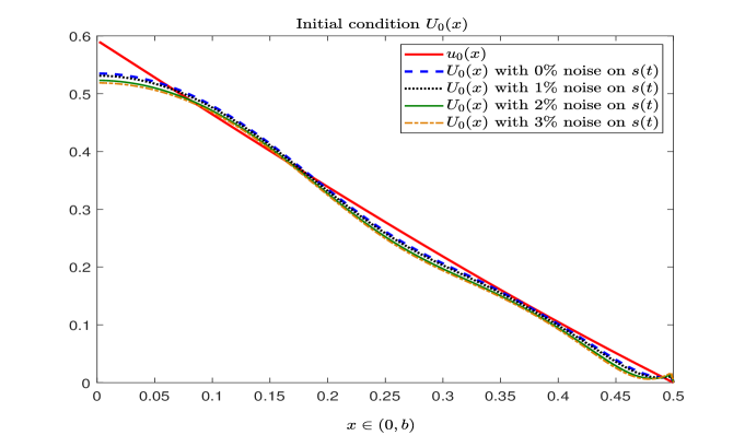
In Figure 4.1, we present the exact initial condition and its reconstruction using the Tikhonov Regularization method. In order to test the stability of our inverse problem, we add a different level of gaussian noise to the data $s(t)$: $1$, $2$ and $3\%$. The Table 1 compiles the relative errors of reconstruction of the function describing the initial condition using the Tikhonov Regularization method. It shows that the accuracy is altered with noise and the relative error on the numerical solution is lower than $0.07$.

Figure 4.2. The exact initial condition $u_{0}(x)$ and approximate solution with different Gaussian noise levels obtained with $M=250$ using Landweber method.

Noise on $s(t)$ ($\%$)	$\frac{\|u_{0}-U_{0}\|_{2}}{\|u_{0}\|_{2}}$
0 $\%$	0.0846
1 $\%$	0.0917
2 $\%$	0.1026
3 $\%$	0.1115

Table 2. Relative errors using Landweber method.

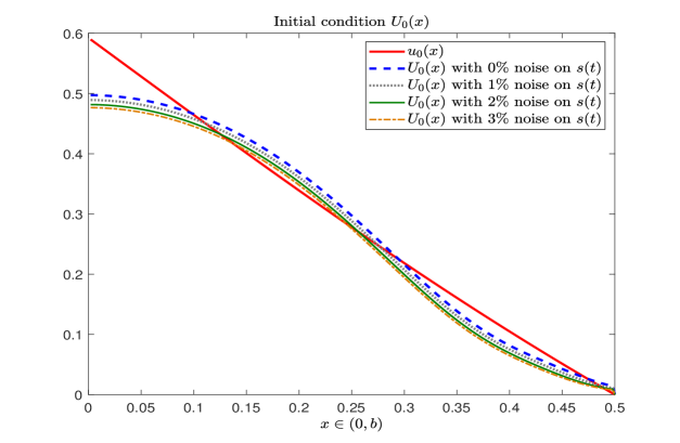
Considering the same example but this time with the Landweber method, the results in the Table 2 show that the relative error of the initial condition $U_{0}(x)$ varies from $8.5\times 10^{-2}$ to $1.1\times 10^{-1}$ by adding $1\%$, $2\%$ and $3\%$ of Gaussian noise on the data $s(t)$. We particularly notice from Tables 1 and 2 that the accuracy of the solution $U_{0}(x)$ with Tikhonov Regularization method is higher compared to the solution obtained with Landweber method.

4.4. Example 2

This example [23] has a moving boundary given by the linear function

(4.10) $$s(t)=\sqrt{2}-1+\frac{t}{\sqrt{2}},\ t\in[0,1].$$

We take the exact solution given by

(4.11) $$u(x,t)=-1+\exp\big{(}1-\frac{1}{\sqrt{2}}+\frac{t}{2}-\frac{x}{\sqrt{2}}\big{)},\ \ [x,t]\in[0,s(t)]\times[0,1].$$

Therefore, this example has the following initial and boundary conditions

(4.12) $$b =s(0)=\sqrt{2}-1,$$

(4.13) $$-u_{x}(0,t) =\frac{1}{\sqrt{2}}\exp\big{(}1-\frac{1}{\sqrt{2}}+\frac{t}{2}\big{)},\ t\in[0,1]$$

(4.14) $$u(s(t),t) =0,\ t\in(0,1],$$

(4.15) $$u_{x}(s(t),t) =\dot{s}(t)=-\frac{1}{\sqrt{2}},\ t\in(0,1].$$

In this example we wish to recover the initial condition at $t=0$ given by

(4.16) $$u_{0}(x)=-1+\exp\big{(}1-\frac{1}{\sqrt{2}}-\frac{x}{\sqrt{2}}\big{)},x\in[0,b].$$

Figure 4.3. The exact initial condition $u_{0}(x)$ and the approximate solution with different Gaussian noise levels obtained with $\lambda=10^{-2}$, $M=250$ using Tikhonov method.

$\lambda$	Noise on $s(t)$ ($\%$)	$\frac{\|u_{0}-U_{0}\|_{2}}{\|u_{0}\|_{2}}$
$10^{-2}$	0 $\%$	0.0953
$10^{-2}$	1 $\%$	0.0997
$10^{-2}$	2 $\%$	0.1082
$10^{-2}$	3 $\%$	0.1465

Table 3. Relative errors using Tikhonov method.

Figure 4.4. The exact initial condition $u_{0}(x)$ and approximate solution with different Gaussian noise levels obtained with $M=250$ using Landweber method.

Noise on $s(t)$ ($\%$)	$\frac{\|u_{0}-U_{0}\|_{2}}{\|u_{0}\|_{2}}$
0 $\%$	0.1017
1 $\%$	0.1188
2 $\%$	0.1321
3 $\%$	0.1520

Table 4. Relative errors using Landweber method.

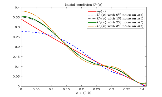
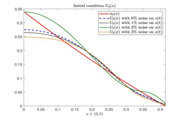
In Figures 4.3 and 4.4, we plotted the exact initial condition and the approximate solution using respectively the Tikhonov and Landweber Regularization methods with different added Gaussian noise levels. The Tables 3 and 4 provide the relative errors of the solution $U_{0}$ using respectively the Tikhonov and Landweber Regularization methods. We remark that the accuracy of the initial condition using Tikhonov Regularization is higher compared to the solution with Landweber method.

4.5. Example 3

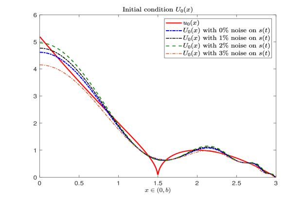
In this numerical test, we consider an example where the analytic solution is not available. We resolve the direct Stefan problem (2.2)-(2.7) with the initial and boundary conditions cited below (4.17) by using the Boundary Immobilisation Method (BIM) [18] in order to calculate the moving boundary $s(t)$. Then we intend to recover the initial temperature $U_{0}(x)$.

(4.17) $$u_{0}(x)=(3-x)\sqrt{\left|3-2x\right|},\ x\in[0,3],\quad\quad h(t)=\sqrt{t+1},\ t\in[0,3].$$

Figure 4.5. The initial condition $u_{0}(x)$ and approximate solution with different Gaussian noise levels obtained with $\lambda=10^{-3}$ and $M=250$ using Tikhonov method.

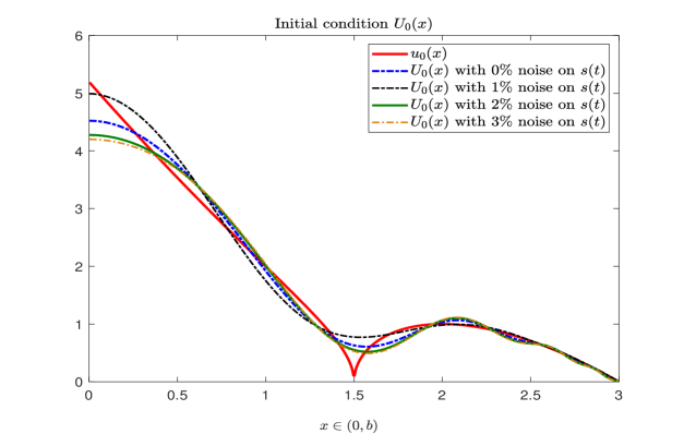
In the Figure 4.5, we present the exact initial condition and the approximate solutions with different added Gaussian noise levels on the data $s(t)$ using the Tikhonov method. From the Table 5, we show that the relative error of the initial condition $U_{0}(x)$ using the Tikhonov Regularization varies from $7.14\times 10^{-2}$ to $1.00\times 10^{-1}$ by adding different levels of Gaussian noise on the data $s(t)$.

$\lambda$	Noise on $s(t)$ ($\%$)	$\frac{\|u_{0}-U_{0}\|_{2}}{\|u_{0}\|_{2}}$
$10^{-3}$	0 $\%$	0.0714
$10^{-3}$	1 $\%$	0.0866
$10^{-3}$	2 $\%$	0.0916
$10^{-3}$	3 $\%$	0.1002

Table 5. Relative errors using Tikhonov method.

We take the same example again but this time with the Landweber method, we notice from the table 6 that the relative error of the initial condition $U_{0}(x)$ varies from $6.90\times 10^{-2}$ to $1.13\times 10^{-1}$ by adding $1\%$, $2\%$ and $3\%$ of Gaussian noise on the data $s(t)$. The exact and approximate solutions for different noise levels using Landweber method are illustrated in Figure 4.6.

Figure 4.6. The initial condition $u_{0}(x)$ and approximate solution with different Gaussian noise levels obtained with $M=250$ using Landweber method.

Noise on $s(t)$ ($\%$)	$\frac{\|u_{0}-U_{0}\|_{2}}{\|u_{0}\|_{2}}$
0 $\%$	0.0690
1 $\%$	0.0755
2 $\%$	0.0970
3 $\%$	0.1132

Table 6. Relative errors using Landweber method.

Remark 4.1.

Notice that in the two first considered examples the explicit initial conditions are analytic functions of the spatial variable. This explains their relatively good recovery far away from the endpoints, from the measurement of the free boundary. In Table 6, we observe that the reconstruction is very sensitive to the noise level. This is in accordance with the obtained stability estimate, and the ill-posedness of the inverse problem.

References

- [1] K. Ammari, A. Bchatnia, and K. El Mufti. A remark on observability of the wave equation with moving boundary. Journal of Applied Analysis, 23(1):43–51, 2017.
- [2] K. Ammari and F. Triki. On weak observability for evolution systems with skew-adjoint generators. SIAM Journal on Mathematical Analysis, 52(2):1884–1902, 2020.
- [3] G. Bruckner and J. Cheng. Tikhonov Regularization for an integral equation of the first kind with logarithmic kernel. Journal of Inverse and Ill-posed Problems, 8(6):665–675, 2000.
- [4] J.R. Cannon and J. Douglas, Jr. The Cauchy problem for the heat equation. SIAM Journal on Numerical Analysis, 4(3):317–336, 1967.
- [5] J.R. Cannon and J. Douglas Jr. The stability of the boundary in a Stefan problem. Annali della Scuola Normale Superiore di Pisa-Classe di Scienze, 21(1):83–91, 1967.
- [6] J.R. Cannon and C.D. Hill. Existence, uniqueness, stability, and monotone dependence in a Stefan problem for the heat equation. Journal of Mathematics and Mechanics, 17(1):1–19, 1967.
- [7] J.R. Cannon and M. Primicerio. Remarks on the one-phase Stefan problem for the heat equation with the flux prescribed on the fixed boundary. Journal of Mathematical Analysis and Applications, 35(2):361–373, 1971.
- [8] M. Choulli. Various stability estimates for the problem of determining an initial heat distribution from a single measurement. arXiv preprint arXiv:1512.07421, 2015.
- [9] M. Choulli and M. Yamamoto. Logarithmic stability of parabolic Cauchy problems. arXiv preprint arXiv:1702.06299, 2017.
- [10] H. W. Engl, M. Hanke, and A. Neubauer. Regularization of inverse problems, volume 375. Springer Science & Business Media, 1996.
- [11] E. Fernández-Cara, F. Hernández, and J. Límaco. Local null controllability of a 1d Stefan problem. Bulletin of the Brazilian Mathematical Society, New Series, 50(3):745–769, 2019.
- [12] E. Fernández-Cara, J. Limaco, and S.B. de Menezes. On the controllability of a free-boundary problem for the 1d heat equation. Systems & Control Letters, 87:29–35, 2016.
- [13] A. Friedman. Partial differential equations of parabolic type prentice-hall inc. Englewood Cliffs, NJ, 1964.
- [14] A. Friedman. Variational Principles and Free Boundary Problems. J. Wiley and Sons, 1992.
- [15] A. Friedman. Partial differential equations of parabolic type. Courier Dover Publications, 2008.
- [16] G.C. Garcia, A. Osses, and M. Tapia. A heat source reconstruction formula from single internal measurements using a family of null controls. Journal of Inverse & Ill-Posed Problems, 21(6):755–779, 2013.
- [17] B. Geshkovski and E. Zuazua. Controllability of one-dimensional viscous free boundary flows. SIAM J. Control Optim., 59(3):1830–1850, 2021.
- [18] C. Ghanmi, S. Mani-Aouadi, and F. Triki. Identification of a boundary influx condition in a one-phase Stefan problem. To appear in Appl. Anal., 2021.
- [19] N.L Gol’dman. Inverse Stefan Problems, volume 412. Springer Science & Business Media, 2012.
- [20] A. Hajiollow, Y. Lotfi, K. Parand, A. H. Hadian, K. Rashedi, and J. A. Rad. Recovering a moving boundary from Cauchy data in an inverse problem which arises in modeling brain tumor treatment: the (quasi) linearization idea combined with radial basis functions (RBFs) approximation. Engineering with Computers, pages 1–15, 2020.
- [21] M. Hanke, A. Neubauer, and O. Scherzer. A convergence analysis of the Landweber iteration for nonlinear ill-posed problems. Numerische Mathematik, 72(1):21–37, 1995.
- [22] P. Jochum. The numerical solution of the inverse Stefan problem. Numerische Mathematik, 34(4):411–429, 1980.
- [23] B.T. Johansson, D. Lesnic, and T. Reeve. A method of fundamental solutions for the one-dimensional inverse Stefan problem. Applied Mathematical Modelling, 35(9):4367–4378, 2011.
- [24] P. Knabner. Control of Stefan problems by means of linear-quadratic defect minimization. Numerische Mathematik, 46(3):429–442, 1985.
- [25] W.T. Kyner. An existence and uniqueness theorem for a nonlinear Stefan problem. Journal of Mathematics and Mechanics, 8(4):483–498, 1959.
- [26] O.A. Ladyzhenskaia, V.A. Solonnikov, and N.N. Ural’tseva. Linear and quasi-linear equations of parabolic type, volume 23. American Mathematical Soc, 1968.
- [27] L. Landweber. An iteration formula for fredholm integral equations of the first kind. American journal of mathematics, 73(3):615–624, 1951.
- [28] J. Li, M. Yamamoto, and J. Zou. Conditional stability and numerical reconstruction of initial temperature. Communications on Pure & Applied Analysis, 8(1):361, 2009.
- [29] R. Nevanlinna, H. Behnke, L.V. Grauert, H.and Ahlfors, D.C. Spencer, L. Bers, K. Kodaira, M. Heins, and J.A. Jenkins. Analytic functions, volume 11. Springer, 1970.
- [30] R. Reemtsen and A. Kirsch. A method for the numerical solution of the one-dimensional inverse Stefan problem. Numerische Mathematik, 45(2):253–273, 1984.
- [31] L. I. Rubinstein. The Stefan problem, volume 8. American Mathematical Soc, 1971.
- [32] W. Rudin. Real and complex analysis. Tata McGraw-hill education, 2006.
- [33] T. Wei and M. Yamamoto. Reconstruction of a moving boundary from Cauchy data in one-dimensional heat equation. Inverse Problems in Science and Engineering, 17(4):551–567, 2009.
- [34] L.C. Wrobel. A boundary element solution to Stefan’s problem. Boundary elements V, page 173, 1983.