Outlier-robust subsampling techniques for persistent homology
Abstract
In recent years, persistent homology (PH) has been successfully applied to real-world data in many different settings. Despite significant computational advances, PH algorithms do not yet scale to large datasets preventing interesting applications. One approach to address computational issues posed by PH is to select a set of landmarks by subsampling from the data. Currently, these landmark points are chosen either at random or using the maxmin algorithm. Neither is ideal as random selection tends to favour dense areas of the data while the maxmin algorithm is very sensitive to noise. Here, we propose a novel approach to select landmarks specifically for PH that preserves coarse topological information of the original dataset. Our method is motivated by the Mayer-Vietoris sequence and requires only local PH computation thus enabling efficient computation. We test our landmarks on artificial datasets which contain different levels of noise and compare them to standard landmark selection techniques. We demonstrate that our landmark selection outperforms standard methods as well as a subsampling technique based on an outlier-robust version of the –means algorithm for low sampling densities in noisy data with respect to robustness to outliers.
Keywords: Landmarks, persistent homology, subsampling, outliers, noise
1 Introduction
One of the practical challenges of applying persistent homology (PH) is that it is computationally difficult for large datasets. Building a filtration on a dataset with points results in spaces of the size , although in practice this can be reduced to by posing a limit on the dimension of the topological features considered (Otter et al., 2017). Following the construction of a filtration, the algorithm for computing PH in the worst case has a complexity of , where is the number of points, edges, triangles, and higher-dimensional connections constructed from the data points by the filtration (the number of such connections can be up to ), although the complexity is often linear in practice (Otter et al., 2017; Edelsbrunner et al., 2002). Methods exist to approximate specific filtrations or to reduce the sizes of the vector spaces associated to the data by a filtration, for an overview of such methods that have been implemented in software packages, see (Otter et al., 2017). Despite such improvements, computation is still very challenging on large datasets and can pose a hard limit on the filtrations that can be applied to a particular dataset. In such cases it can become necessary to preprocess data before applying PH. For point cloud data one can, for example, use subsampling techniques to identify so-called landmarks of the dataset and then define a filtration on the landmarks (de Silva and Carlsson, 2004). A filtration on well chosen landmarks retains topologically important global information about the full dataset and one can even choose to include information from non-landmark points when constructing the filtration. An example for such a filtration is the lazy witness filtration which was first introduced by (de Silva and Carlsson, 2004) and has been used to study noisy artificial datasets (Kovacev-Nikolic, 2012), primary visual cortex cell populations (Singh et al., 2008), and cancer gene expression data (Lockwood and Krishnamoorthy, 2015). Roughly, the lazy witness filtration consists of the following steps111For the full definition see (de Silva and Carlsson, 2004).:
-
1.
Selection of a (small) subset222Although there is no systematic lower bound for the number of landmark points, (de Silva and Carlsson, 2004) suggest using of the data points as landmarks. of landmark points from the dataset .
-
2.
Construction of a lazy witness filtration on the landmarks where the landmarks are vertices and data points from the full dataset can serve as witnesses for higher order interactions between sets of landmarks in the filtration.
Even though the choice of landmarks from the data inevitably has a large influence on the results that can be obtained, currently there are only two standard approaches to select landmarks: uniform random selection and selection via the maxmin algorithm. Neither is ideal and in particular the maxmin algorithm tends to include outliers (de Silva and Carlsson, 2004; Adams and Tausz, 2015), which poses problems since large real-world datasets often include noise. In the biological application of the lazy witness filtration in (Lockwood and Krishnamoorthy, 2015), for example, the maxmin algorithm leads to the discovery of loops in the dataset which we could not reproduce using uniform random landmark selection or when discarding a small proportion of the initially chosen maxmin landmarks from the dataset and choosing a new set of landmarks with the maxmin algorithm. We also note that the results of the lazy witness filtration are difficult to interpret. In addition to the mentioned disadvantages of the maxmin algorithm, neither of the proposed landmark selection methods were designed specifically for PH. While there are other methods that address subsampling for PH (Cohen-Steiner et al., 2007; Niyogi et al., 2008; Dufresne et al., 2019) these do not explicitly consider noisy data. Because existing approaches are not ideal, it is desirable to develop new methods that lead to a reduction of large and noisy data while preserving topological properties. Ideally, the reduced dataset can be used as input for PH directly without additional preprocessing steps.
While one of the appeals of PH is its ability to study multi-scale datasets globally, local PH around a data point can also produce useful insights, see for example (Bendich et al., 2012; Ahmed et al., 2014; Fasy and Wang, 2016; Stolz et al., 2020; Wheeler et al., 2021). Here, we present a novel landmark selection technique that allows us to obtain outlier-robust PH landmarks from noisy point cloud data. Our method is motivated by the Mayer–Vietoris sequence and relies on computing the Vietoris–Rips filtration (Carlsson, 2009; Ghrist, 2008) locally, in a small neighbourhood around each data point, where the aforementioned computational problems of PH vanish. Our algorithm then uses PH output to define a score for each data point which allows us to identify suitable candidates for landmarks. We investigate two different flavours of our approach, one using high scores to identify candidate landmarks and one using low scores. We apply our approach to very simple artificial datasets that consist of signal points sampled from an object with a topologically interesting structure, such as a sphere, a torus, or a Klein bottle, as well as noise points. A consequence of the inclusion of noise is that a large dataset cannot be reduced by applying subsampling techniques developed to infer the (persistent) homology of data (Cohen-Steiner et al., 2007; Niyogi et al., 2008; Dufresne et al., 2019). The (global) PH of landmarks selected in our proposed method is close to the PH of signal points in the original dataset. In comparison to existing landmark selection procedures, we demonstrate that our landmarks based on local PH perform very well on our datasets, in particular for low sampling densities, with respect to robustness to outliers. We further investigate the performance of our landmarks in comparison with an outlier-robust version of the –means algorithm (Chawla and Gionis, 2013) which we modify for landmark selection and again find that they are superior for low sampling densities. Our PH landmarks present a valuable addition to the two existing techniques for landmarks selection for PH and we believe that they may also be of interest in a broader data science context.
Local homology has previously been used to infer the stratification of data (Bendich et al., 2012; Mileyko, 2021; Nanda, 2020; Robinson et al., 2018; Stolz et al., 2020) as well as road network analysis (Ahmed et al., 2014; Fasy and Wang, 2016) and, more recently, the analysis of topological complexity of data as it passes through different layers of neural networks (Wheeler et al., 2021). A similar Mayer-Vietoris sequence as the one that motivates our landmark selection approach has been used to show Wasserstein stability bounds of the Vietoris-Rips filtration on finite point clouds (Skraba and Turner, 2020) and local computations motivated by the Mayer-Vietoris sequence have also been applied with the goal of parallelising PH computations (Casas, 2019). Although the idea behind our notion of local persistent homology is similar to some of those used previously (Ahmed et al., 2014; Bendich et al., 2012; Fasy and Wang, 2016; Wheeler et al., 2021), in comparison to these approaches, our definition does not use relative homology and can be readily computed by considering the Vietoris–Rips complex on points in a small local neighbourhood.
Our paper is structured as follows: in Section 2, we review existing standard techniques for landmark selection. We then mathematically motivate and introduce our novel landmark selection technique, which we refer to as PH landmarks, and also present an outlier-robust version of the –means algorithm (Chawla and Gionis, 2013) modified for landmark selection, landmarks, in Section 3. In Section 4 we introduce our datasets. We compare our PH landmarks to existing techniques as well as landmarks in Section 5 followed by a discussion in Section 6.
2 Existing landmark selection methods
The two standard methods for selecting landmarks in a dataset are random landmark selection and the maxmin algorithm. Both are implemented as standard procedures for use in combination with the lazy witness filtration in the PH software package javaPlex (Tausz et al., 2014).
2.1 Random landmark selection
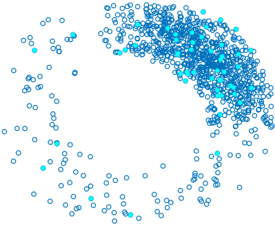
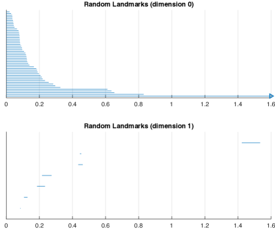
The simplest way to choose landmarks from a point cloud is to select points from uniformly at random. For datasets whose points are evenly distributed, random selection achieves good coverage at a small computational cost. However, as soon as there are large differences in the density of the data, random selection will favour points from more dense regions, which can result in landmarks that do not represent the point cloud well. In extreme cases, the landmarks do not carry any topological similarity to the original point cloud. We show such an example in Fig. 1.
2.2 The maxmin algorithm
The sequential maxmin algorithm chooses the first landmark randomly. Inductively, for and a landmark set , the algorithm selects the next landmark such that for a chosen metric with the function mapping
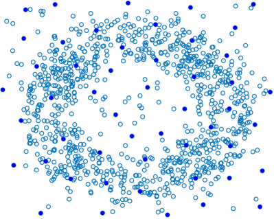
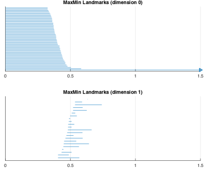
is maximised for . We show pseudocode for the procedure in Algorithm 3 in Appendix A.1. The method has been used successfully for image data in (Adams and Carlsson, 2009; Carlsson et al., 2008). Landmarks chosen in this way cover the dataset well, are evenly spaced, and represent the underlying topological features better than landmarks selected at random. The algorithm does, however, tend to include outliers (de Silva and Carlsson, 2004; Adams and Tausz, 2015). We show an example of a point cloud where the selected landmarks do not represent the underlying topology of the data correctly in Fig. 2.
According to (de Silva and Carlsson, 2004), the maxmin algorithm is best suited to produce the qualities desired from landmarks. They do not recommend the use of clustering algorithms as an alternative due to the high computational cost and potential to accentuate accidental features.
2.3 Dense core subsets
The tutorial accompanying the PH software package javaPlex (Adams and Tausz, 2015) mentions that using so-called dense core subsets before applying the maxmin algorithm can help overcome the selection of outliers as landmarks. This approach, however, is not considered as one of the standard approaches for landmark selection and we did not find examples where it was used in practice for this purpose. De Silva and Carlsson, 2004 and Carlsson et al., 2008 apply dense core subsets to identify dense regions in their datasets. The authors subsequently use the maxmin landmarks to study the topology of these dense regions.
Dense core subsets are based on assigning density values to every point: for an integer , the density value assigned to a point is , where is the distance to the -th nearest neighbour of . Large values of provide a measure of the global density around the point in the dataset, while smaller values of give a more local perspective. Using the density values, one can select the densest points in the dataset as a dense core subset. Given a dataset, it is not clear what values of to use. Different values for and can produce markedly different subsets (de Silva and Carlsson, 2004).
For our comparisons in Subsection 5.3, instead of selecting a dense subset and then performing the maxmin algorithm to select landmarks, as proposed by (Adams and Tausz, 2015), we choose the densest points in the data as landmarks. This enables us to determine how the information on which our own landmark selection technique (PH landmarks) is based differs from that given by the -th nearest neighbour of a data point.
3 Proposed landmark selection methods
Currently existing methods for landmark selection that enable subsequent PH analysis on large and noisy point cloud data are not ideal and have, in particular, not been designed with PH in mind. De Silva and Carlsson, 2004 state the most pertinent qualities for a landmark set to be good coverage of the dataset and even spacing spacing of the landmarks. While these are certainly important properties for many datasets, we find that in the context of PH, regardless of whether the landmarks are intended for use in combination with the lazy witness complex or simply as a subset of the dataset to apply PH to, the aim of a landmark selection method should be to represent the underlying topology of the dataset. Since outliers can artificially introduce topological features such as loops, we in particular require outlier-robust landmark selection techniques. Based on these observations we formulate the following goals for landmark selection methods intended for PH:
-
1.
Good representation of the underlying topology of the dataset, even at low sampling densities with small variance of the results between different landmark realisations.
-
2.
Robustness to outliers, ideally including a measure for how much we consider a specific point to be an outlier.
We now introduce novel landmark selection methods to achieve these goals: Persistent homology landmarks (PH landmarks) and landmarks. We design PH landmarks specifically for the application of PH, while landmarks are based on a variant of the –means algorithm, whose outlier-robust properties make it a promising candidate to overcome the downsides of both the random and the maxmin landmark selection.
3.1 Mathematical motivation
The use of our notion of local PH is inspired by the Mayer-Vietoris sequence, which can enable computation of the homology of a space by considering subspaces, whose homology is easier to compute. The Mayer-Vietoris sequence for a topological space is a special type of long exact sequence. By long exact sequence we mean a sequence of abelian groups and group homomorphisms , , of the form
| (1) |
such that . For more definitions and background, see for example (Munkres, 1984)).
Theorem 1 (Mayer-Vietoris sequence)
Let be a simplicial complex with subcomplexes such that . Then there exists an exact sequence
| (2) |
where denotes the -th homology group and , , and are homomorphisms. The sequence is called the Mayer-Vietoris sequence.
For a proof see, for example, (Munkres, 1984), page 142. We can use the Mayer-Vietoris sequence to connect the homology of a simplicial complex to the local homology around a vertex . We do this via two simplicial subcomplexes that can be defined around the vertex : the link of the vertex and the closed star of the vertex .
Definition 2 (Closed star of a vertex)
Let be a simplicial complex and a vertex. Then the closed star of in , denoted by , is the subcomplex of that contains all the simplices which have as one of their vertices.
Definition 3 (Link of a vertex)
Let be a simplicial complex and a vertex. Then the link is the union of all simplices of lying in that are disjoint from .
We show a simplicial complex, the closed star of a vertex and the link of a vertex in Fig. 3.

Denoting the simplicial complex of all simplices in that are disjoint from as , we make the following observations for :
Remark 4
-
1.
.
-
2.
.
Based on these definitions and observations we can now consider the following Mayer-Vietoris sequence:
| (3) |
Now, is contractible: every simplex that contains is contractible and the intersection of simplices in is either empty or a simplex that contains and is hence also contractible. Thus for . We observe that if we can ensure that , for we obtain:
| (4) |
which gives us an isomorphism between and .
The Mayer-Vietoris sequence given by Eq. 3 connects the homology of the large simplicial complexes and , which are both global and expensive to compute, to the homology of the Link , which a purely local computation and therefore easy to compute.
In practice, we are however working with point cloud data . We therefore consider the PH of the point cloud , rather than the homology, and apply the Mayer-Vietoris sequence 3 to the simplicial complexes that we obtain from the data by constructing a filtration. We consider a simplicial complex in this filtration. A data point is now a vertex in . Instead of , we need to quantify the failure of the isomorphism via a score based on the , which we will define in Section 3.2. To make computation easier, instead of looking just at the link of in the simplicial complex , we extend the link to a -neighbourhood of in , which we define to be the collection of simplices whose vertices are within a distance of at most from in :
Definition 5 (-link of a data point )
Let be a simplicial complex in a metric space constructed from a dataset , a vertex, a distance and a -neighbourhood of in . Then the -link is the union of all simplices in that are disjoint from and contained in .
Building on the -Link of a data point we can define the -Star of a data point:
Definition 6 (Closed -star of a data point )
Let be a simplicial complex in a metric space constructed from a dataset , a vertex, a distance and a -neighbourhood of in . Then the closed -star is the union of the -link with the vertex and all simplices where and is fully contained in .
We note that the closed -star of a data point is always contractible by construction. We show an example of a data point, its -link and its closed -star in Fig. 4.
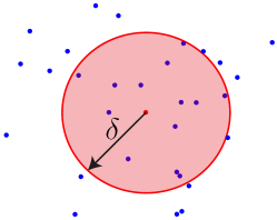
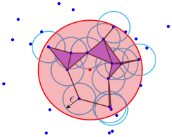
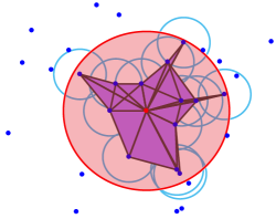
From now on, we refer to computing the PH of the -Link of a point in a dataset as computing the local PH of a data point. Our notion of local PH of a data point is motivated by the Mayer-Vietoris sequence and we use the property given by Eq. 4 to define a new landmark selection method, in which we select points in a dataset which are ‘closest’ to giving us the desired isomorphism between and as landmarks. Note that a similar computation for local PH is performed in Wheeler et al. (2021).
3.2 Persistent homology landmarks
Following our local PH computations, we can now define the score by which we measure the failure of the isomorphism .
Definition 7 ()
Let be a point cloud, a data point, a distance function, , and the -dimensional barcode of the Vietoris–Rips filtration performed on excluding infinitely persisting features. Then
We can reformulate our observation from Eq. 4 for point cloud data and PH in the following way: if for a data point and a neighbourhood radius we can ensure that , then for we obtain:
| (5) |
where denotes the -th homology groups associated with the different filtration steps. As we are working with data however, we are unlikely to achieve such strict conditions – indeed, we would achieve these under trivial conditions. For , however, we obtain something close to an isomorphism between and .
The larger of a point is, the further away we are from an isomorphism between and . Consequently, the inclusion or exclusion of the point changes the PH of the dataset more than for a point where is small. Under the assumption that each point has at least two neighbours within distance , the choice of determines by how much we allow the Bottleneck distance (for a definition see, for example, (Otter et al., 2017)) between the persistence diagrams of the filtration on the point cloud containing and a point cloud not containing to differ. We can therefore think of it as a resolution parameter. There are now two possible strategies for landmark selection:
-
•
PH landmarks I: representative landmarks. Landmarks are points with small values. Their inclusion or exclusion in the full dataset does not alter the PH of the full dataset dramatically. Hence, the landmarks represent the data well and they do not introduce accidental topological features that can, for example, be caused by outlier points in the landmark set.
-
•
PH landmarks II: vital landmarks. Landmarks are points with large values. For such points we are far away from an isomorphism between and . Hence their exclusion from the dataset would change the PH dramatically.
In practice, it is not immediately clear which strategy works better. Here, we therefore consider both. We compute for dimensions . Motivated by results from our computations, we define two versions for which we use in practice. To avoid confusion with Definition 7, we refer to these values obtained in practical computations as the PH outlierness of a point :
| (6) |
where is the length of the longest finite interval in the PH barcode for dimension . We also refer to as outlierness over all (computed) dimensions. We observe that is usually determined by dimension 0, where we find the longest non-infinitely persisting features in our datasets (see Subsection 5.1). To avoid this, we also use a version for PH outlierness which is restricted to dimension 1 in the PH calculation:
| (7) |
We also refer to as dimension 1 outlierness. In situations where either of the two definitions can be used, we denote PH outlierness as .
To avoid choosing points as landmarks that are very far away from other data points, we determine points with fewer than two neighbours within their -neighbourhood to be super outliers. We include super outliers into the landmark set only once all other points have been chosen as landmarks. Note that the resolution parameter strongly influences the number of super outliers. As long as we have enough points in the dataset that are not considered to be super outliers, we choose our landmarks to be the points such that for all and for PH landmarks I (representative landmarks) and for all and for PH landmarks II (vital landmarks). We show the pseudocode for PH landmarks I in Algorithm 1, an algorithm for PH landmarks II can be formulated accordingly.
When using in Algorithm 1, it is important to note, that one can obtain data points that are not super outliers with . To avoid that the order of inclusion of such points in the landmark set is determined by a possibly systematic and non-random ordering of the points in the original dataset, which could, for example, favour noise points to be added before signal points or vice versa, we ensure that all points with are randomly permuted in the ordering of the PH outlierness scores.
3.3 landmarks
The –means algorithm was developed by (Chawla and Gionis, 2013) to overcome the extreme sensitivity of the –means algorithm to outliers. The authors formulate their approach as a generalisation of the –means algorithm: for an input dataset the algorithm provides a set of cluster centres and a set of outliers , . For a given distance function and the authors use the following term in their algorithm:
| (8) |
We show the pseudocode in Algorithm 4 in Section A.2. For our application of the algorithm to landmark selection, we further define:
| (9) |
We show our modified version of the –means algorithm for landmark selection in Algorithm 2.
3.4 Implementation
We implement PH landmark selection method in Matlab using Ripser (Bauer, ; Bauer, 2021) for the computation of the local Vietoris–Rips complexes. We also implement the landmarks algorithm in Matlab. For the calculation of maxmin landmarks, random landmarks, and dense core subsets we use the inbuilt functions in the javaPlex package (Tausz et al., 2014).
4 Datasets
We introduce the datasets to which we apply the different landmark selection methods. The datasets are chosen to be simple to allow us to determine effects of the landmark selection. The datasets consist of signal points that are sampled from a topologically interesting structure – a sphere, a Klein bottle, or a torus – and noise points that we design to be topologically different from the signal.
4.1 3-dimensional datasets
4.1.1 Sphere-cube dataset.
For a given number of points and probability we sample signal points uniformly at random from the surface of the unit sphere with probability and noise points from the (filled) cube with probability .
4.1.2 Sphere-plane dataset
For a given number of points we sample signal points uniformly at random from the surface of the unit sphere with probability and noise points from the -plane with probability .
4.1.3 Sphere-line dataset
For a given number of points we sample signal points uniformly at random from the surface of the unit sphere with probability and noise points from , where , with probability .
4.1.4 Sphere-Laplace line dataset
For a given number of points we sample signal points uniformly at random from the surface of the unit sphere with probability and we sample noise points from with probability , where is sampled from and Laplace distributed with and . We use the Laplacian random number generator code (Chen, 2019) to generate .
4.2 4-dimensional datasets
4.2.1 Torus dataset
We use the following parametrisation of the torus :
where . We add noise to the torus using the equation
where .
For a given number of points we sample signal points uniformly at random from with probability and noise points from with probability .
4.2.2 Klein bottle dataset
We use the following parametrisation of the Klein bottle :
where , and . We define noise for the Klein bottle using the equations:
where is sampled uniformly from the interval and is sampled uniformly from the interval . We use and adapt the code from (Otter et al., 2017). For a given number of points we sample signal points uniformly at random from with probability and noise points from with probability .
5 Results
We present our results for the proposed landmark selection methods, i.e. PH landmarks and landmarks. We first study PH landmark selection in detail on the sphere-cube dataset with , then proceed to showing our results in comparison to the current standard methods on our various datasets, i.e. landmark selection via the maxmin algorithm and random landmark selection. We then compare our methods to dense core subsets and finally investigate the influence of the parameter on the performance of PH landmarks. For all landmark selection techniques we use the Euclidean distance as distance function. All of our datasets consist of 3000 points.
5.1 PH landmarks case study on the sphere-cube dataset with
We apply PH landmark selection with to the sphere-cube dataset where a data point has a probability of 0.6 to be located on the surface of the unit sphere and 0.4 to be located in the unit cube. As for all of our datasets, we find that the PH outlierness values , as defined in Eq. 6, are determined by the maximal non-infinite bar in the dimension barcode. We show example barcodes for dimension 0 for a noise point, a sphere point, and a super outlier in Fig. 5. In general, we expect a noise point to be located in a sparser region of this dataset and thus to either be classified as a super outlier, or to exhibit a barcode with a small number of long bars and very few, or no, short bars. For a sphere point, we expect the dimension 0 barcode to have many short bars and occasionally some longer bars caused by noise points that lie within the -neighbourhood. Note that for the examples in Fig. 5, we choose the noise point with the highest outlierness score and the sphere point with the lowest outlierness score in the dataset to illustrate model cases for the method.
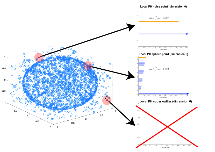
We find that for these example points, the dimension 0 barcodes behave as expected. To explore whether the outlierness scores reflect the properties of the different types of points as expected, we consider histograms of the outlierness scores of all data points in Fig. 6.
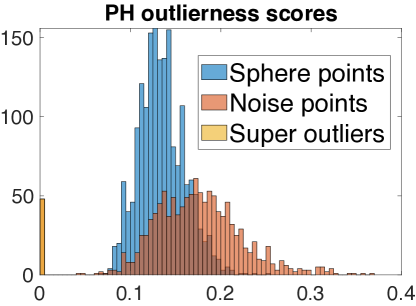
We find that we have 48 super outliers in the dataset. For the noise and sphere points, we can see that the outlier scores are distributed differently and that by including points with low outlier scores as landmarks first, we should preferentially obtain sphere points rather than noise points. Landmarks chosen in this way correspond to representative landmarks (PH landmarks I) described in Subsection 3.2.
As our landmark selection approach is motivated by Eq. 5 which holds for PH in dimensions , it is not immediately clear that representative landmarks are preferable to vital landmarks both for and dimensions . We examine a variant of the method where we restrict ourselves to local PH in dimension 1. In this case dimension 1 PH outlierness values correspond to the persistence of the most persistent feature in the local dimension 1 barcode (see Eq. 7). We show a histogram of the distribution of the dimension 1 PH outlierness scores in Fig. 7.
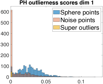
We observe that the clearest difference between the sphere points and the noise points is the fact that a large proportion of noise points has , while a clear majority of the sphere points has . This can again be explained by the fact that sphere points have more neighbours within their -neighbourhood and therefore are more likely to form features in dimension 1. From these observations it seems that here it is more beneficial to use vital landmarks (PH landmarks II), described in Subsection 3.2, for landmark selection based on dimension 1. For PH landmarks based on dimension 1 we thus choose points with large dimension 1 PH outlierness scores as landmarks and discard points with low dimension 1 PH outlierness scores from the dataset as outliers whose removal does not alter the PH of the dataset much.
5.2 Comparison of persistent homology landmarks and landmarks to standard landmark selection methods
We compare our proposed methods for landmark selection, the landmarks and the PH landmarks, to the current standard methods for landmark selection, i.e. random landmarks and maxmin landmarks. Using the different techniques we choose landmarks from data points. This corresponds to a landmark sampling density of . For the landmarks, we define the number of clusters to be and the number of outliers to be , where is the probability with which a point in the respective dataset was sampled from the signal data, i.e. the sphere, torus, or Klein bottle. We consider both the case where we choose the cluster centres and the outliers found by the algorithm as our landmarks as well as the case where we only consider the cluster centres to be landmarks. For the PH landmarks we choose for the 3-dimensional datasets, for the torus data and for the Klein bottle. In all our datasets, we find that when looking for the maximal persistence of a feature across all dimensions, the value of is exclusively determined by dimension 0. We therefore also include a variation of PH landmarks that only considers the local dimension 1 barcode for the calculation of . For the PH landmark version where we use all dimensions to determine the outlierness scores, we choose data points with small as our landmarks (representative landmarks), for the version where we restrict ourselves to dimension 1, we choose points with large scores as landmarks (vital landmarks).
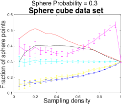
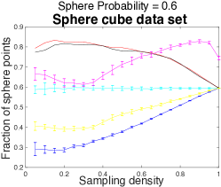
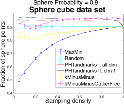
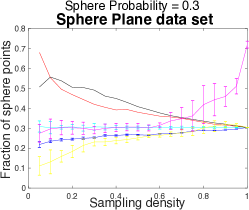
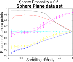
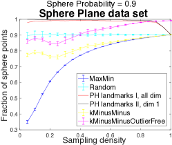
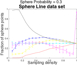
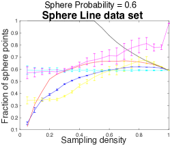
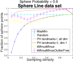
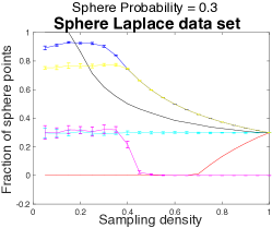
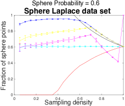
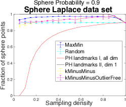
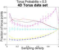
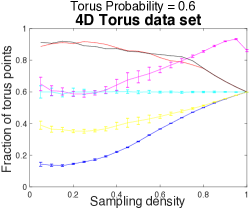
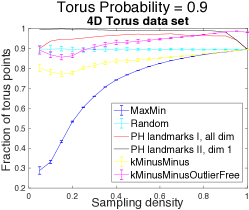
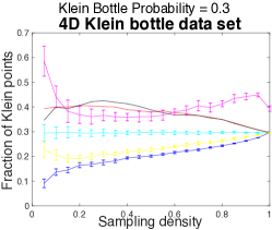
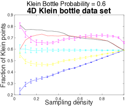
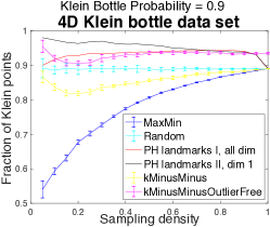
For all our datasets, our aim for the landmarks is to contain a high fraction of signal points, even when sampling only a small fraction of the data as landmarks. In Figures 8–13 we show plots of the fraction of signal points in the various landmark sets at different sampling densities. Since in the PH landmark selection we allow super outliers as landmarks once all other points are taken, we expect the fraction of signal landmarks for sampling density 1 to represent the probability of signal points in the dataset, except in the variant of the landmarks where we include only the cluster centres as landmarks (referred to as ‘kMinusMinusOutlierFree’ in the plots). Note that for this variant of landmarks for datasets with , it is possible to obtain a signal fraction of even for sampling density 1 if the algorithm selects all cluster centres to be located among noise points. For the maxmin, random and landmarks we show the average fraction of signal points and its standard deviation across 20 realisations of the selection algorithms.
As expected, we observe that the maxmin algorithm tends to select noise points as landmarks for all datasets with only one exception (see Figures 8–13): for the sphere-Laplace data, the maxmin algorithm performs well (see Fig. 11), as the noise is located in a cluster far away from the signal and hence maximising the distance between landmarks results in many points being selected from the sphere. The fraction of signal landmarks for random selection also behaves as we expect for all datasets in Figures 8–13: the selected landmarks are representative for the whole dataset with an almost constant fraction of signal points over all sampling densities that corresponds to the fraction of signal points in the dataset. For the landmarks, we can see a clear improvement in the signal fraction in most datasets in Figures 8–13 when considering only cluster centres as landmarks – the inclusion of outliers gives the landmarks similarly bad properties as the maxmin landmarks. The landmarks that do not include outliers tend to perform well for high sampling densities, where the number outlier points corresponds roughly to the number of noise points in the dataset. For low sampling densities however, the method only outperforms random selection for most of the sphere-cube and Klein bottle datasets (see Figures 8 and 13). For the sphere-plane, sphere-line and the sphere Laplace-line datasets the reason for this lies in the nature of the noise, which leads to the selection of cluster centres in the noise data. We also notice large standard deviations from the average fraction of signal points in the landmark over 20 realisations.
With exception of the sphere-line and sphere-Laplace datasets (see Figures 10 and 11), the PH landmark selection techniques I and II both outperform the standard methods as well as the landmarks clearly for most cases, especially for low sampling densities. Interestingly, the landmarks perform very well on the Klein bottle dataset (see Fig. 13), beating both PH landmarks for very small sampling densities. For the sphere-line and sphere-Laplace datasets (see Figures 10 and 11), PH landmarks II restricted to dimension 1 outperform all other methods for low sampling densities while PH landmarks I across all dimensions perform worse than all other methods in most cases. The noise in these datasets is located on lines in dense regions of the dataset where the local PH does not find any topological features in dimension 1, but many features with low persistence in dimension 0. In general, the two versions of PH landmarks start coinciding as soon as super outliers are added to the dataset which we can observe in the plots as a rapid drop in the fraction of signal points. We add the super outliers to the landmarks in random order (once all other points are already selected as landmarks) and hence both PH landmark methods differ only slightly in the development of their signal fractions after the addition of super outliers. We note there are cases in which the PH landmarks thrive because the points that are not super outliers are predominantly signal points. This is not the case for the sphere-line and the sphere-Laplace datasets with (see Figures 10 and 11) for which the dimension 1 PH landmarks II perform very well. Both of these datasets have less than 4 super outliers. Interestingly, there seems to be a trend for the dimension 1 PH landmarks II to outperform PH landmarks I on datasets with high signal content, i.e. for across all datasets. For lower signal content the PH landmarks I perform strongly. For the Klein bottle dataset, dimension 1 PH landmarks II outperform PH landmarks I in almost all cases.
Overall, the results underline that both PH landmarks I and II represent the PH of the dataset well and are robust to outliers, in particular for low sampling densities. They outperform standard methods in a large majority of cases and, moreover, via the PH outlierness score they give us a notion of how much a point can be considered an outlier for the respective variant of the method. landmarks perform better than random selection in most cases and perform very well, in particular, for high sampling densities. Given the much higher computational cost and the large fluctuations in signal fraction between different realisations of the method, using random selection instead of landmarks could however present a more practical approach.
5.3 Comparisons between persistent homology landmark selection methods and dense core subsets
We now provide a more in detail study of the two PH landmark selection techniques, in particular concerning the influence of the parameter. We also compare the techniques to two dense core subsets, using for and , which we consider as landmark sets. We present our results in Figures 14 – 19. We present only the plots for datasets with a signal probability .
For the dense core subsets, we find that for all datasets except the sphere-plane, sphere-line, and sphere-Laplace datasets (see Figures 15 – 17) the local density measure outperforms the more global density measure . Indeed, in these cases, the dense core subset with captures a larger fraction of signal points than most of our PH landmarks. For the sphere-cube dataset (see Fig. 14), we seem to outperform the dense core subset with for a small range of low sampling densities for , which is a value where most of the data points are classified as super outliers. Our definition of super outliers as points with less than two neighbours in their -neighbourhoods, seems to imply that, for this dataset, the distance to the second closest neighbour is more relevant for low sampling densities than the distance to the closest neighbour. Interestingly, for the datasets where the local dense core subset with performs well (see Figures 14, 18, and 19 ), we also see that smaller values of give us better results, both for PH landmarks I across all dimensions and PH landmarks II restricted to dimension 1. For the sphere-line dataset (see Fig. 16), where we have a better performance for the dense core subset with , larger -neighbourhoods are more advantageous for both PH landmark versions. In this case, we perform as well as the dense core subset with for for dimension1 PH landmarks II. In the sphere-Laplace dataset (see Fig. 17) PH landmarks II clearly outperform both dense core subsets. Here again, we find the trend that larger values are advantageous for PH landmarks II. The fact that dense core subsets perform well on most of our datasets is determined by our signal points lying in denser regions of the data than the noise points. It is only in the sphere-Laplace dataset (see Fig. 17), where the noise does not obey this characteristic and we observe that the local PH information in this case is richer than the distance to the -th neighbour.
Finally, we show how the number of super outliers depends on the choice of in Fig. 20. We observe that small values lead to a drastic increase in the proportion of super outliers in the dataset. This underlines that, even though one can think of as a resolution parameter, depending on the dataset, the proportion of super outliers is an important factor to consider.
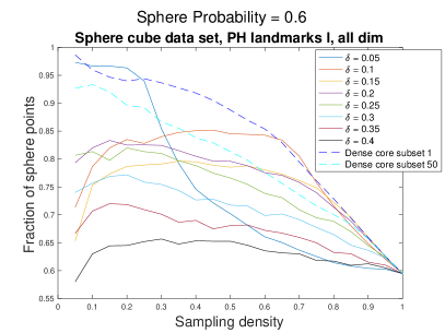
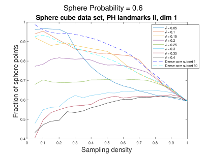
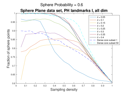
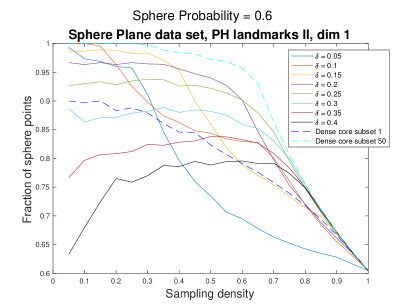
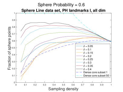
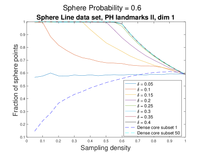
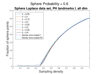
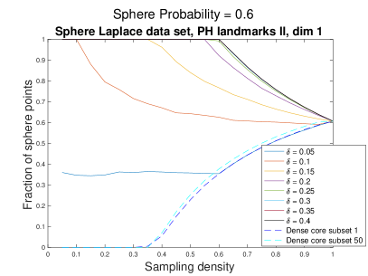
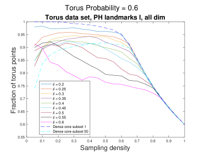
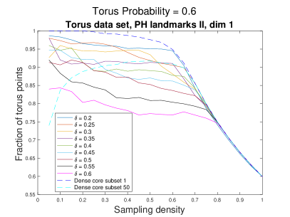
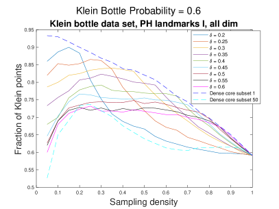
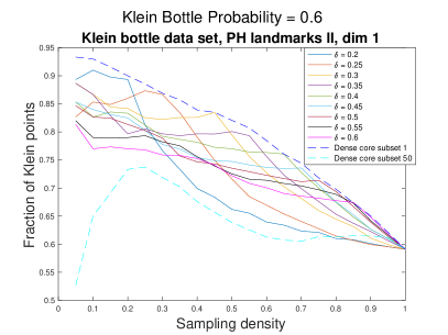
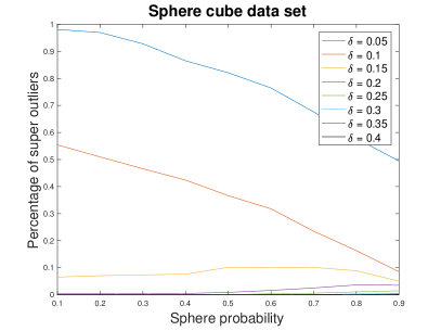
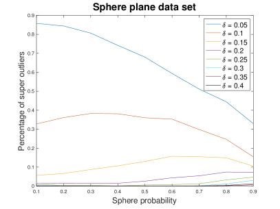
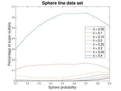
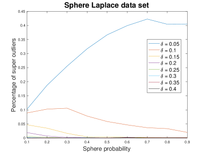
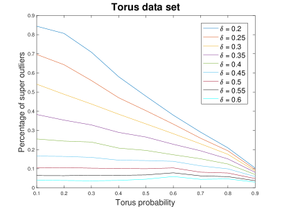
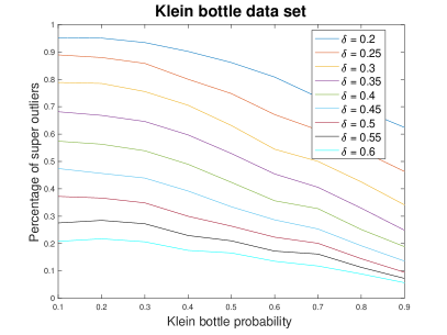
Overall, PH landmarks outperform all standard techniques on most datasets as well as two dense core subsets on the sphere-Laplace for a broad range of -values. To obtain signal fractions that are high and stable over a long range of low sampling densities we recomment to choose as small as possible without having too many super outliers in the data.
6 Discussion
We proposed novel outlier-robust landmark selection techniques: landmarks and two versions of PH landmarks. PH landmark selection is the first landmark selection method developed specifically for the use of PH.
The landmarks outperformed existing standard landmark selection methods – random selection and maxmin selection – in many cases. They however tended to do so for large sampling densities, which are not very relevant for data subsampling. While landmarks did meet our goals for an outlier-robust landmark selection technique, this algorithm has a high computational cost and is difficult to use on a dataset with unknown properties as one has to predetermine the number of outliers for the algorithm to find.
We found that both versions of PH landmarks outperformed the existing standard landmark selection techniques on datasets containing noise, in particular for low landmark sampling densities. We observed this for a wide range of resolution values. In most of our datasets, PH landmarks II (vital landmarks) restricted to dimension 1 for calculating the outlierness values slightly outperformed the PH landmarks I (vital landmarks) considering all dimensions (which coincides with a restriction to dimension 0 in our cases) for datasets with a high signal content and a low noise content, while PH landmarks I performed better for higher noise content.
Dimension 1 PH landmarks II further outperformed dense core subsets showing that the method can capture richer information than just considering the -th nearest neighbour as shown on the sphere-Laplace dataset. On our other datasets, both versions of PH landmarks were outperformed by dense core subsets due to the fact that in these datasets the signal points tend to be located in denser parts of the data than noise points. Overall, however, we consider PH landmarks to be a more practical approach than dense core subsets since they only require the choice of one parameter, . In contrast, when applying dense core subsets as suggested in (Adams and Tausz, 2015), one needs to choose the parameter to obtain a density estimate, followed by the number of densest points to be chosen from the dataset, which are then used to obtain maxmin landmarks. In (de Silva and Carlsson, 2004), the authors observed that when studying dense core subsets the choices of parameters can indeed result in strong topological differences in the selected point clouds. With only one parameter choice we expect both versions of PH landmarks to deliver more consistent results.
In practice, we hypothesise that PH landmarks II using will lead to better results in high-dimensional data, especially in cases where signal data is sparse. The parameter would then have to be large enough to ensure that local PH in dimension 1 produces non-trivial barcodes for a large proportion of data points. For very large datasets with potentially high noise content, calculating or even a version restricted to dimension 0 for PH landmarks I could therefore be computationally advantageous.
We believe that PH landmarks contribute a valuable alternative to the current standard landmark selection techniques for PH, in particular for noisy datasets. The PH outlierness values as well as the number of super outliers with respect to the resolution could further be used to provide interesting insight into datasets for exploratory data analysis and could be incorporated in novel data analysis techniques which aim to take properties of shape of the data into account without performing computationally expensive PH analyses of the full dataset. Identifying representative and vital landmarks in datasets could be of interest to study processes underlying the data, for example in biology. While methods from Machine Learning are excellent at classifying such data, the underlying mechanisms often remain hidden to these methods and results by themselves can be difficult to interpret. Building on our work, it would be interesting to investigate different definitions of PH outlierness in future studies. Testing the applicability of PH landmarks to real-world datasets with different types of noise or different levels of sparsity will be the subject of future work.
Acknowledgments
The author is very grateful for feedback and input from Vidit Nanda, Jared Tanner, and Heather Harrington as well as helpful suggestions from Scott Balchin. BJS is a member of the Centre for Topological Data Analysis, funded by the EPSRC grant (EP/R018472/1), and acknowledges funding from the EPSRC and MRC (EP/G037280/1) as well as F. Hoffmann-La Roche AG during her doctoral studies.
A Appendix
A.1 Pseudocode for maxmin algorithm (Adams and Tausz, 2015)
A.2 Pseudocode for –means algorithm (Chawla and Gionis, 2013)
References
- Adams and Carlsson (2009) Henry Adams and Gunnar Carlsson. On the nonlinear statistics of range image patches. SIAM Journal on Imaging Sciences, 2(1):110–117, 2009.
- Adams and Tausz (2015) Henry Adams and Andrew Tausz. JavaPlex tutorial. Available at http://javaplex.googlecode.com/svn/trunk/reports/javaplex_tutorial/javaplex_tutorial.pdf, 2015.
- Ahmed et al. (2014) Mahmuda Ahmed, Brittany Terese Fasy, and Carola Wenk. Local persistent homology based distance between maps. In Proceedings of the 22nd ACM SIGSPATIAL International Conference on Advances in Geographic Information Systems, pages 43–52. ACM, 2014.
- (4) Ulrich Bauer. Ripser: a lean c++ code for the computation of Vietoris–Rips persistence barcodes. Software available at https://github.com/Ripser/ripser, software retrieved in 2017.
- Bauer (2021) Ulrich Bauer. Ripser: efficient computation of vietoris-rips persistence barcodes. Journal of Applied and Computational Topology, 2021. doi: 10.1007/s41468-021-00071-5.
- Bendich et al. (2012) Paul Bendich, Bei Wang, and Sayan Mukherjee. Local homology transfer and stratification learning. In Proceedings of the twenty-third annual ACM-SIAM symposium on Discrete Algorithms, pages 1355–1370. SIAM, 2012.
- Carlsson (2009) Gunnar Carlsson. Topology and data. Bulletin of the American Mathematical Society, 46:255–308, 2009.
- Carlsson et al. (2008) Gunnar Carlsson, Tigran Ishkhanov, Vin De Silva, and Afra Zomorodian. On the local behavior of spaces of natural images. International Journal of Computer Vision, 76(1):1–12, 2008.
- Casas (2019) Álvaro Torras Casas. Distributing persistent homology via spectral sequences. arXiv preprint arXiv:1907.05228, 2019.
- Chawla and Gionis (2013) Sanjay Chawla and Aristides Gionis. k-means–: A unified approach to clustering and outlier detection. In Proceedings of the 2013 SIAM International Conference on Data Mining, pages 189–197. SIAM, 2013.
- Chen (2019) Elvis Chen. Laplacian random number generator. Available at: https://www.mathworks.com/matlabcentral/fileexchange/13705-laplacian-random-number-generator, March 2019.
- Cohen-Steiner et al. (2007) David Cohen-Steiner, Herbert Edelsbrunner, and John Harer. Stability of persistence diagrams. Discrete and Computational Geometry, 37(1):103–120, 2007.
- de Silva and Carlsson (2004) Vin de Silva and Gunnar Carlsson. Topological estimation using witness complexes. In Markus Gross, Hanspeter Pfister, Marc Alexa, and Szymon Rusinkiewicz, editors, SPBG’04 Symposium on Point - Based Graphics 2004, pages 157–166. The Eurographics Association, 2004.
- Dufresne et al. (2019) Emilie Dufresne, Parker Edwards, Heather Harrington, and Jonathan Hauenstein. Sampling real algebraic varieties for topological data analysis. In 2019 18th IEEE International Conference On Machine Learning And Applications (ICMLA), pages 1531–1536. IEEE, 2019.
- Edelsbrunner et al. (2002) Herbert Edelsbrunner, David Letscher, and Afra Zomorodian. Topological persistence and simplification. Discrete and Computational Geometry, 28:511–533, 2002.
- Fasy and Wang (2016) Brittany Terese Fasy and Bei Wang. Exploring persistent local homology in topological data analysis. In IEEE International Conference on Acoustics, Speech and Signal Processing (ICASSP), pages 6430–6434. IEEE, 2016.
- Ghrist (2008) Robert Ghrist. Barcodes: The persistent topology of data. Bulletin of the American Mathematical Society, 45:61–75, 2008.
- Kovacev-Nikolic (2012) Violeta Kovacev-Nikolic. Persistent homology in analysis of point-cloud data. Master’s thesis, University of Alberta, https://era.library.ualberta.ca/files/cv43nx33b/Kovacev-Nikolic_Violeta_Fall2012.pdf, 2012.
- Lockwood and Krishnamoorthy (2015) Svetlana Lockwood and Bala Krishnamoorthy. Topological features in cancer gene expression data. In Pacific Symposium on Biocomputing, pages 108–119, 2015.
- Mileyko (2021) Yuriy Mileyko. Another look at recovering local homology from samples of stratified sets. Journal of Applied and Computational Topology, 5(1):55–97, 2021.
- Munkres (1984) James R. Munkres. Elements of algebraic topology. The Benjamin/Cummings Publishing Company, inc., Redwood City (California), Menlo Park (California), Reading (Massachusetts), Amsterdam, Don Mills (Ontario), Mexico City, Sydney, Bonn, Madrid, Singapore, Tokyo, Bogota, Santiago, San Juan, Wokingham (United Kingdom), 1984.
- Nanda (2020) Vidit Nanda. Local cohomology and stratification. Foundations of Computational Mathematics, 20(2):195–222, 2020.
- Niyogi et al. (2008) Partha Niyogi, Stephen Smale, and Shmuel Weinberger. Finding the homology of submanifolds with high confidence from random samples. Discrete and Computational Geometry, 39(1-3):419–441, 2008.
- Otter et al. (2017) Nina Otter, Mason A. Porter, Ulrike Tillmann, Peter Grindrod, and Heather A. Harrington. A roadmap for the computation of persistent homology. European Physical Journal – Data Science, 6(17):1–38, 2017.
- Robinson et al. (2018) Michael Robinson, Chris Capraro, Cliff Joslyn, Emilie Purvine, Brenda Praggastis, Stephen Ranshous, and Arun Sathanur. Local homology of abstract simplicial complexes. arXiv preprint arXiv:1805.11547, 2018.
- Singh et al. (2008) Gurjeet Singh, Facundo Mémoli, Tigran Ishkhanov, Guillermo Sapiro, Gunnar Carlsson, and Dario L. Ringach. Topological analysis of population activity in visual cortex. Journal of Vision, 8(11):1–18, 2008.
- Skraba and Turner (2020) Primoz Skraba and Katharine Turner. Wasserstein stability for persistence diagrams. arXiv preprint arXiv:2006.16824, 2020.
- Stolz et al. (2020) Bernadette J. Stolz, Jared Tanner, Heather A. Harrington, and Vidit Nanda. Geometric anomaly detection in data. Proceedings of the National Academy of Sciences, 117(33):19664 – 19669, 2020. ISSN 0027-8424. doi: 10.1073/pnas.2001741117. URL https://www.pnas.org/content/early/2020/07/31/2001741117.
- Tausz et al. (2014) Andrew Tausz, Mikael Vejdemo-Johansson, and Henry Adams. JavaPlex: A research software package for persistent (co)homology. In Han Hong and Chee Yap, editors, Mathematical Software. ICMS 2014, volume 8592 of Lecture Notes in Computer Science, pages 129–136. Springer, Berlin, Heidelberg, 2014. Software available at http://appliedtopology.github.io/javaplex/.
- Wheeler et al. (2021) Matthew Wheeler, Jose Bouza, and Peter Bubenik. Activation landscapes as a topological summary of neural network performance. arXiv preprint arXiv:2110.10136, 2021.