LiGCN: Label-interpretable Graph Convolutional Networks
for Multi-label Text Classification
Abstract
Multi-label text classification (MLTC) is an attractive and challenging task in natural language processing (NLP). Compared with single-label text classification, MLTC has a wider range of applications in practice. In this paper, we propose a label-interpretable graph convolutional network model to solve the MLTC problem by modeling tokens and labels as nodes in a heterogeneous graph. In this way, we are able to take into account multiple relationships including token-level relationships. Besides, the model allows better interpretability for predicted labels as the token-label edges are exposed. We evaluate our method on four real-world datasets and it achieves competitive scores against selected baseline methods. Specifically, this model achieves a gain of 0.14 on the F1 score in the small label set MLTC, and 0.07 in the large label set scenario.
1 Introduction
In the real world, we have seen an explosion of information on the internet, such as tweets, micro-blogs, articles, blog posts, etc. A practical issue is to assign classification labels to those instances. Such labels may be emotion tags for tweets and micro-blogs Wang et al. (2016); Li et al. (2020b), or topic category tags for news, articles and blog posts Yao et al. (2019). Multi-label text classification (MLTC) is the problem of assigning one or more labels to each instance.
| Text | Labels | |
|---|---|---|
| S1 | 我不知道类似这样的困惑到底还要持续多久。 (I don’t know how long the confusion like this will last.) | Anxiety |
| S2 | nothing happened to make me sad but i almost burst into tears like 3 times today | Pessimism, Sadness |
| S3 | …The price of BASF AG shares improved on Thursday due to its better than expected half year results. At 0900 GMT BASF was up 51 pfennigs at 42.75 marks… | C15, C151, C152, CCAT |
Deep learning has been applied for MLTC due to their strong representation capacity in NLP tasks. It has been shown that convolutional neural networks (CNNs) Kim (2014) achieve satisfying results for multi-label emotion classification Wang et al. (2016); Feng et al. (2018). Besides, many recurrent neural networks (RNNs)-based models Tang et al. (2015) are also playing an important role Huang et al. (2019); Yang et al. (2018). Recent breakthrough of pre-trained models, i.e., BERT Devlin et al. (2019) and RoBERTa Liu et al. (2019a), achieved large performance gains in many NLP tasks. Existing work has applied BERT to solve MLTC problem successfully with very competitive performances Li et al. (2019c). Moreover, as a new type of neural network architecture with growing research interest, graph convolutional networks (GCNs) Kipf and Welling (2017) have been applied to multiple NLP tasks. Different from CNN and RNN-based models, GCNs could capture the relations between words and texts if modeled as graphs Yao et al. (2019); Li et al. (2019a, 2020a). In the paper, we focus on emphasising a GCN-based model to solve MLTC task.
A major challenge for MLTC is the class imbalance. In practice, the number of labels may vary across the training data, and the frequency of each label may differ as well, bringing difficulties to model training Quan and Ren (2010). In Table 1, we show some examples of tweet, micro-blog and news article, labeled with emotion tags or news topics. As can be seen from those examples, there is a various number of coexisting labels. Another challenge is the interpretation of assigned class labels by figuring out the trigger words and phrases to corresponding labels. In the table, it is easy to tell that in S1, the emotion Anxiety is very likely to be triggered by the word confusion. However, S2 might be more complicated, with two possible triggering phrases makes me sad and burst into tears and two emotion labels. There might be different opinions on which phrase triggers which emotion.
To tackle the mentioned challenges and investigate different perspectives, we propose label-interpretable graph convolutional networks for MLTC. We model each token and class label as nodes in a heterogeneous graph, considering various types of edges: token-token, token-label, and label-label. Then we apply graph convolution to graph-level classification. As GCN works well in semi-supervised learning Ghorbani et al. (2019), we can then ease the impact of data imbalance. Finally, since the token-label relationships are exposed in the graph, one can easily identify the triggering tokens to a specific class, providing a good interpretability for multi-label classification.
The contributions of our work are as follows: (1) We transfer the MLTC task to a link prediction task within a constructed graph to predict output labels. In this way, our model is able to provide token-level interpretation for classification. (2) To the best of our knowledge, this is the first work that considers token-label relationships within a manner of a graph neural network for MLTC, allowing label interpretability. (3) We conduct extensive experiments on four representative datasets and achieve competitive results. We also demonstrate comprehensive analysis and ablation studies to show the effectiveness of our proposed model for label nodes and token-label edges. We release our code in https://github.com/IreneZihuiLi/LiGCN.
2 Related Work
Multi-label Text Classification Many existing works focus on single-label text classification, while limited literature is available for multi-label text classification. In general, these methods fall into three categories: problem transformation, label adaptation and transfer learning. Problem transformation is to transform the muli-label classification task into a set of single-label tasks Jabreel and Moreno (2019); Fei et al. (2020), but this method is not scalable when the label set is large. Label adaptation is to rank the predicted classes or set a threshold to filter the candidate classes. Chen et al. (2017) proposed a novel method to apply an RNN for multi-label generation with the help of text features learned using CNNs. Transfer learning focuses on utilizing knowledge learned to unknown entries. Xiao et al. (2021) proposed a model which transfers the meta-knowledge from data-rich labels to data-poor labels. Moreover, some models also take label correlations into consideration, such as Seq2Emo Huang et al. (2019) and EmoGraph Xu et al. (2020). However, some of them may ignore the relationships between input tokens and class labels, making them less interpretable. Please note that there is a research topic named extreme multi-label text classification Liu et al. (2017), where the pool of candidate labels is extremely large. However, we do not target on the extreme case.
Graph Neural Networks in NLP Previous research has introduced GCN-based methods for NLP tasks by formulating them as graph-structured data tasks. A fundamental task is text classification. Many works show that it is possible to utilize inter-relations of documents or tokens to infer the labels Yao et al. (2019); Zhang et al. (2019). Besides, some NLP tasks focus on learning relationships between nodes in a graph, such as concept prerequisites Li et al. (2019a) and leveraging dependency trees predicted by GCNs for machine translation Bastings et al. (2017). Recently, variations of GCN models have been investigated for general text classification tasks Linmei et al. (2019); Tayal et al. (2019); Ragesh et al. (2021). Limited efforts have been made to apply GCNs for multi-label text classification. For example, EmoGraph Xu et al. (2020) is a model that captures the dependencies among emotions through graph networks.
3 Method
In this section, we first provide task definition and preliminary, then we introduce the proposed model for multi-label text classification.
3.1 Task Definition
In multi-label text classification task, we are given the training data . For the -th sample, contains a list of tokens and is a list of binary labels , is 1 if the class label is positive, 0 otherwise. The size of label set can be small or large. In testing, we predict labels given .
3.2 Preliminary
Graph convolutional network (GCN) Kipf and Welling (2017) is a type of deep architecture for graph-structured data. In a typical GCN model, we define a graph as , where is a set of nodes and is a set of edges. Normally, the edges are represented as an adjacency matrix , and the node representation is defined as . In a multi-layer GCN, the propagation rule for layer is defined as:
| (1) |
where is a normalization function, denotes the node representation, and is the parameter matrix to be learned. , denotes the degree matrix of , In general, in the very first layer, we have .
3.3 Label-interpretable Graph Convolutional Networks
In this paper, we propose the LiGCN model, which allows interpretation on the labels when doing MLTC. For each training sample, we construct an undirected graph. We define two types of nodes: token node and label node, and the node representations are and . Therefore, there are three types of relations between the nodes, defined by the adjacency matrices: (between token nodes), (between label nodes) and (between token nodes and label nodes).
We show the model overview in Figure 1. It consists of two main components: a pre-trained BERT/RoBERTa encoder111https://huggingface.co/bert-base-multilingual-cased,
https://huggingface.co/roberta-base and label-node graph convolutional layers. In the LiGCN model, we have a list of token nodes in orange ellipses, and a list of label nodes in blue ellipses. Besides, there are edges between token nodes , edges between label nodes , and edges between token and label nodes . We explain them in greater details below.
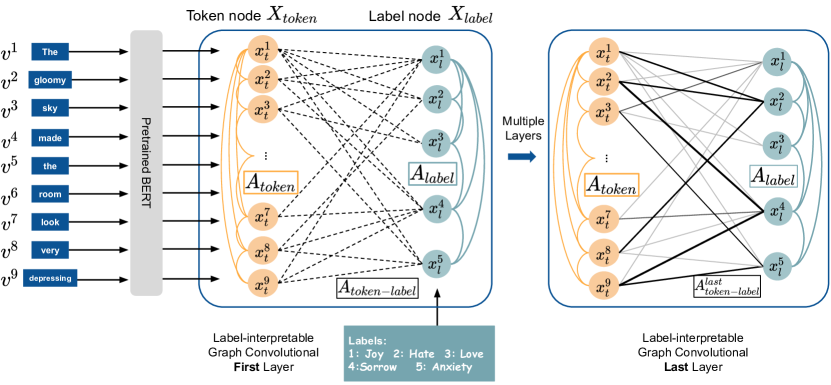
Node Representations : In the very first layer, to initialize token nodes, we encode the input data using a pre-trained BERT or RoBERTa model and possible other BERT-based ones, where we take the representation of each token including [CLS] token as . For the label nodes, we initialize them using one-hot vectors.
Adjacency Matrix : In our experiments, to initialize token node adjacency matrix , we use the token nodes to construct an undirected chain graph, where we consider an input sequence as its natural order, i.e., in : . Since it is an undirected graph, the adjacency matrix is symmetric, i.e., . We also add self-loop to each token: . In other words, is a symmetric -by- matrix with an upper bandwidth of 1, where is the number of token nodes.
We initialize with an identity matrix, and with a zero matrix. In the later layers, we reconstruct for layer by applying cosine similarity between and of the current layer:
| (2) |
The value is normalized into the range of [0,1]. After this update, the model conducts graph convolution operation as in Eq. 1.
In Figure 1, we are not showing self-loops, so is not visible. We show only a subset of edges from and . Note that we use dashed lines at the first LiGCN layer because is a zero matrix.
We also investigate other possible ways to build including dependency parsing trees Huang et al. (2020) and random initialization, but our method gives the best result. Such ways may not bring useful information to the graph: the help from dependency relations may be limited in the case of classification, and random initialization brings noises. As we focus more on the network convolution, we leave investigating more methods for initialization as future work.
| Dataset | #train | #dev | #test | #class | #avg label | #token max | #token median | #token mean |
|---|---|---|---|---|---|---|---|---|
| SemEval | 6,839 | 887 | 3,260 | 11 | 2.37 | 499 | 26 | 32.08 |
| RenCECps | 27,299 | - | 7,739 | 8 | 1.37 | 36 | 17 | 16.42 |
| RCV1 | 20,647 | 3,000 | 783,144 | 103 | 3.20 | 9,380 | 198 | 259.06 |
| AAPD | 54,840 | - | 1,000 | 54 | 2.41 | 500 | 157 | 166.41 |
Predictions In the last LiGCN layer, we are able to reconstruct using Eq. 2. For each label node , we sum up the edge weights from to get a score,
| (3) |
where is the set of all token nodes in the last LiGCN layer. Then we apply a softmax function over all the labels, so that the scores are transformed to probabilities of labels. Finally, to make the prediction, we rank the probabilities in a descending order, and keep the top labels from the ranking as predictions. As the predictions are in forms of probabilities, we also convert the ground truths into probability distribution. We use the mean square error (MSE) as the loss function. Another way is to apply the normal cross-entropy for classification, but it achieves slightly worse results, so we do not include it.
4 Experimental Results
We evaluate on four public datasets, summarized in Table 2 and 3: SemEval Mohammad et al. (2018) contains a list of subtasks on labeled tweets data. In our experiments, we focus on Task1 (E-c) challenge on English corpus: multi-label classification tweets on 11 emotions. RenCECps Quan and Ren (2010) is a Chinese blog corpus which contains manual annotation of eight emotional categories. It not only provides sentence-level emotion annotations, but also contains word-level annotations, where in each sentence, emotional words are highlighted. RCV1 Lewis et al. (2004) consists of manually-labeled English news articles from Reuters Ltd. Each news article has a list of topic class labels, i.e., CCAT for Corporate/industrial, G12 for Internal politics. We follow the same setting of Yang et al. (2018) and Nam et al. (2017), and do MLTC on the top 103 classes. AAPD Yang et al. (2018) is a set of English computer science paper abstracts and corresponding subjects from arxiv.org.
| #label | SemEval | RenCEPcs | RCV1 | AAPD |
|---|---|---|---|---|
| 0 | 293 | 2,755 | 0 | 0 |
| 1 | 1,481 | 18,858 | 35,591 | 0 |
| 2 | 4,491 | 11,417 | 203,030 | 38,763 |
| 3 | 3,459 | 1,815 | 362,124 | 12,782 |
| 4 | 1,073 | 172 | 85,527 | 3,229 |
| 186 | 21 | 120,518 | 1,066 | |
| Avg. | 2.37 | 1.37 | 3.20 | 2.41 |
We report the following evaluation metrics:
Micro/Macro F1, Jaccard Index We report micro-average and macro-average F1 scores as did by previous works Baziotis et al. (2018); Huang et al. (2019) if the label set is small. Besides, we follow the Jaccard index used by Mohammad et al. (2018); Baziotis et al. (2018); Huang et al. (2019), as always referred as multi-label accuracy. The definition is given below:
where is the number of samples, denotes the ground truth labels and denotes system predicted labels.
P@k and nDCG@k When the label set is large, we also report widely-applied metrics P@K and nDCG@K ().
We apply two graph convolutional layers for all datasets by default for our LiGCN model. In Table 4, we show the hyper-parameters conducted in our experiments. We use 4.00E-06 as the learning rate for all experiments. Since we use two LiGCN layers, hid dim1 is the first layer hidden dimension number, and hid dim2 is the second layer hidden dimension number. These hyper-parameters were selected by dev sets (if exist), otherwise selected by manual tuning with about 5-10 rounds for search trials.
| SemEval | RenCECPs | RCV1 | AAPD | |
|---|---|---|---|---|
| seq length | 17 | 32 | 256 | 256 |
| hid dim1 | 64 | 64 | 256 | 256 |
| hid dim2 | 16 | 16 | 64 | 64 |
| epoch num | 5 | 3 | 10 | 10 |
| top- | 2 | 1 | 5 | 5 |
| SemEval | RenCECps | ||||||
| Method | Macro F1 | Micro F1 | Jaccard | Macro F1 | Micro F1 | Jaccard | |
| SGM Yang et al. (2018) | 0.4110 | 0.5750 | 0.4820 | - | 0.5560 | - | |
| Seq2Emo Huang et al. (2019) | - | 0.7089 | 0.5919 | - | - | - | |
| TECap Fei et al. (2020) | 0.5760 | 0.6820 | - | 0.4550 | 0.5310 | - | |
| MEDA Deng and Ren (2020) | - | - | - | 0.4831 | 0.6076 | - | |
| EmoGraph (BERT-GCN)*Xu et al. (2020) | 0.6367 | 0.8108 | 0.6818 | 0.6129 | 0.8559 | 0.7481 | |
| BERT | 0.5223 | 0.6454 | 0.4766 | 0.5344 | 0.6365 | 0.4669 | |
| RoBERTa | 0.5039 | 0.6817 | 0.5171 | 0.5842 | 0.7987 | 0.6649 | |
| BERT-LiGCN (ours) | 0.7368 | 0.8312 | 0.7111 | 0.7138 | 0.8615 | 0.7567 | |
| RoBERTa-LiGCN (ours) | 0.7786 | 0.8579 | 0.7512 | 0.7429 | 0.8756 | 0.7787 | |
| Method | P@1 | P@3 | P@5 | nDCG@3 | nDCG@5 | F1-score |
|---|---|---|---|---|---|---|
| RCV1 | ||||||
| XML-CNN Liu et al. (2017) | 95.75 | 78.63 | 54.94 | 89.89 | 90.77 | 75.92 |
| Imprinting Qi et al. (2018) | 77.38 | 47.96 | 31.45 | 58.83 | 57.91 | 26.35 |
| DXML Zhang et al. (2018) | 94.04 | 78.65 | 54.38 | 89.83 | 90.21 | 75.76 |
| OLTR Liu et al. (2019b) | 93.79 | 61.36 | 44.78 | 74.37 | 77.05 | 56.44 |
| BBN Zhou et al. (2020) | 94.61 | 77.98 | 54.25 | 88.97 | 89.68 | 78.65 |
| HTTN Xiao et al. (2021) | 95.86 | 78.92 | 55.27 | 89.61 | 90.86 | 77.72 |
| BERT-LiGCN (ours) | 94.42 | 80.98 | 55.48 | 91.93 | 91.94 | 83.14 |
| RoBERTa-LiGCN (ours) | 95.61 | 82.40 | 56.31 | 93.40 | 93.26 | 83.66 |
| AAPD | ||||||
| XML-CNN Liu et al. (2017) | 74.38 | 53.84 | 37.79 | 71.12 | 75.93 | 65.35 |
| Imprinting Qi et al. (2018) | 68.68 | 38.22 | 23.71 | 55.30 | 55.67 | 25.58 |
| DXML Zhang et al. (2018) | 80.54 | 56.30 | 39.16 | 77.23 | 80.99 | 65.13 |
| OLTR Liu et al. (2019b) | 78.96 | 56.28 | 38.60 | 74.66 | 78.58 | 62.48 |
| BBN Zhou et al. (2020) | 81.56 | 57.81 | 39.10 | 76.92 | 80.06 | 66.73 |
| HTTN Xiao et al. (2021) | 83.84 | 59.92 | 40.79 | 79.27 | 82.67 | 69.25 |
| BERT-LiGCN (ours) | 84.10 | 61.33 | 40.88 | 80.77 | 83.68 | 75.89 |
| RoBERTa-LiGCN (ours) | 82.50 | 61.26 | 41.38 | 80.39 | 83.83 | 76.25 |
4.1 Small Label Sets
We first evaluate the proposed model on SemEval and RenCECps in Table 5. Both of them have a small label set, so we report Macro, Micro F1 and Jaccard. We select the following baselines: SGM Yang et al. (2018) applies a sequence generation model and a decoder structure; Seq2Emo Huang et al. (2019) is an LSTM-based model that takes into account the correlations among target labels; TECap Fei et al. (2020) is a topic-enhanced capsule network, which contains a variational autoencoder and a capsule module for multi-label emotion detection; MEDA Deng and Ren (2020) is a multi-label emotion detection architecture that focuses on detecting all emotions shown in the text, and it takes BERT for sentence encoding. Finally, EmoGraph Xu et al. (2020) is a graph-based method that learns dependencies among emotion nodes using GCNs. The result presented is based on our implementation with optimized parameters, and is slightly better than their original paper. We also compare with a BERT and a RoBERTa model as baselines (BERT, RoBERTa). We first take the representation of [CLS] token from pre-trained BERT/RoBERTa, on top of that, a linear layer is connected. For the two datasets, we set the top- value to be the average number of labels in each dataset.
We can observe that our model surpasses all the selected baselines in most of the cases. Especially, both MEDA and EmoGraph applied pre-trained BERT model as our BERT-LiGCN model does, and we significantly outperform those models on all three metrics. Moreover, EmoGraph is a similar model with LiGCN but it only considers a single node type (class node) while LiGCN considers both class node and token node. This shows that, with a much complex graph structure, LiGCN is able to capture more information when doing classification. Besides, LiGCN benefits from using RoBERTa as the encoder, as RoBERTa improves upon BERT by a small margin.
| SemEval | RenCECps | ||||||
|---|---|---|---|---|---|---|---|
| BERT-LiGCN | Macro F1 | Micro F1 | Jaccard | Macro F1 | Micro F1 | Jaccard | |
| 1-layer | 0.7131 | 0.8159 | 0.6891 | 0.7054 | 0.8091 | 0.6794 | |
| 2-layer | 0.7368 | 0.8312 | 0.7111 | 0.7138 | 0.8615 | 0.7567 | |
| 3-layer | 0.7109 | 0.8145 | 0.6871 | 0.7044 | 0.8085 | 0.6785 | |
4.2 Large Label Sets
We then evaluate large label sets using RCV1 and AAPD, shown in Table 6. We compare with a number of recent baselines: XML-CNN Liu et al. (2017) applied a CNN and dynamic pooling to learn features for MLTC; Imprinting Qi et al. (2018) is a weight imprinting method that directly set the final layer weights of deep models from new training examples; DXML Zhang et al. (2018) focused on label co-occurrence graph to solve the multi-label long-tail issue; OLTR Liu et al. (2019b) is a method that handles long-tail and imbalanced classification problems; BBN Zhou et al. (2020) is a model that considers both representation learning and classifier learning; HTTN Xiao et al. (2021) learns the meta-knowledge so as to transfer from data-rich head labels to data-poor ones. We set the top- value to be in the prediction so as to evaluate P@ and nDCG@.
Our model can also surpass the selected baselines in general, especially with a large improvement on the F1-score for the two datasets. Surprisingly, BERT-LiGCN performs better than RoBERTa-LiGCN on P@1, P@3 and nDCG@3 in AAPD. In other words, BERT-LiGCN can predict better top-3 candidates, while RoBERTa-LiGCN can do well in predicting the 4-th and 5-th candidates. But in both BERT and RoBERTa settings, our model can perform close and better compared with these recent baselines.
5 Analysis
In this section, we first focus on ablation study of the proposed model. We then demonstrate the interpretability for labels with several case studies where we identify keywords that trigger certain labels. Moreover, we study and examine the meaning of label representations learned by the model.
5.1 Ablation Study
We first study the impact of graph convolutional layer numbers in Table 7. We test with 1, 2 and 3 LiGCN layers on SemEval and RenCECps using BERT-LiGCN model. In general, we see that 2-layer is the best setting. Less layers may not be enough for information exchange within nodes in the GCN models. While increasing the layer number results in training difficulties and lower performances, as some other works Li et al. (2018) have shown.
5.2 Token-label Relations
As our proposed model provides token-label relations, we further study token-level explanations via case studies and a quantitative analysis.
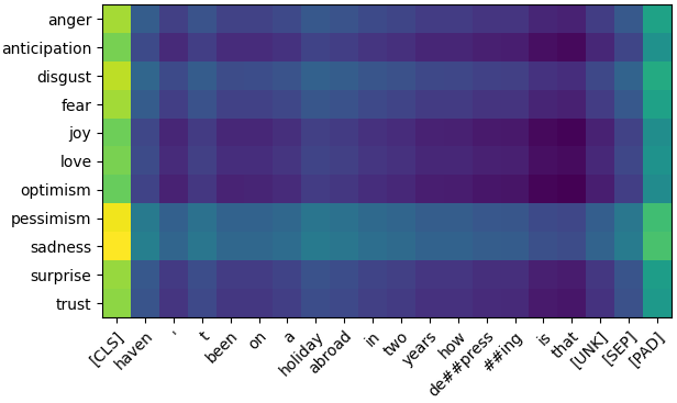
Case Study We show examples by visualizing the token-label weights in Figure 2. Specifically, we take the reconstructed and normalize the matrix so that all values sum up to 1. We select a sample from SemEval test set, as shown in Figure 2(a): haven’t been on a holiday abroad in two years how depressing is that… (labels: pessimism and sadness). In such a heatmap, columns are tokens while rows are the emotion labels. We can notice that our model computes a higher score to the text chunk haven’t and holiday abroad, and a relatively lower score to depressing, by looking at the corresponding columns. Therefore, the prediction being pessimism and sadness is mostly triggered by haven’t and holiday abroad. This indicates that the emotion label to be such a negative sentiment is because this person ‘haven’t been on a holiday abroad.’Even though there is a strong negative sentiment word depressing, LiGCN attempts to pick out implicit and deeper reasons. Besides, one can see that our model highlights other three close emotions anger, disgust and fear. 222When doing classification, both special tokens of BERT [CLS] and [SEP] contain useful semantic information of the whole sequence, so the color tends to be brighter.
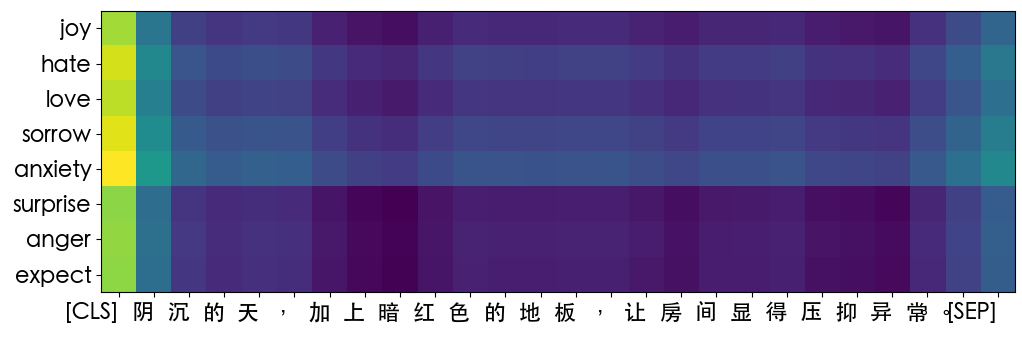
We show another example from RenCECps test set in Figure 2(b): 阴沉的天,加上暗红色的地板,让房间显得压抑异常。 (The gloomy sky, together with the dark red floor, made the room look very depressing.) The ground truth labels are Sorrow and Anxiety. Our model successfully predicts these two class labels; moreover, the model also suggests that Hate is a possible label, which is reasonable in this particular example. Besides, in the annotation of the original dataset by Quan and Ren (2010), we find that two keywords are highlighted for this example: 阴沉 (gloomy) : Surprise=0, Sorrow=0, Love=0, Joy=0, Hate=0, Expect=0, Anxiety=0.6, Anger=0; and 压抑 (depressing): Surprise=0, Sorrow=0.5, Love=0, Joy=0, Hate=0, Expect=0, Anxiety=0.7, Anger=0. Our model also captures such a trend successfully by showing a higher score near or on these token columns.
Quantitative Analysis So far, we have demonstrated that our model is able to identify the triggering words for each individual class from the confidence score of the token-label edges. To quantitatively show the quality of identified triggering words, we compute MSE between our best performed model and the ground truth annotations for the test set of RenCECps. Similar to previous analysis, we first normalize the constructed token-label adjacency matrix , then construct a token-label matrix from ground truth annotations (for each sentence, there is only a few keywords, we assign zero to other non-keyword tokens). Then we are able to compute MSE score between the two aforementioned matrices: . We also reconstruct the token-label matrix from the BERT+single model as a comparison. RoBERTa has an MSE score of 0.0901 and RoBERTa-LiGCN has 0.0020. RoBERTa-LiGCN has a significant lower MSE score compared with RoBERTa. The T-test between the two models based on the predictions is 0.016, showing a significant difference. Since other datasets do not contain token-level annotations, so we fail to conduct quantitative analysis on them.
Highlighted Tokens Additionally, in Table 8, we show a case study selected from AAPD. We keep the top tokens highlighted only. This article is correctly classified as logic in computer science(cs.lo), programming languages (cs.pl) and software engineering (cs.se), marked by different colors. One can notice that the highlighted tokens are closely related to the class fields: object-oriented software and Object Programs are associated with cs.se; reference expressions is associated with cs.pl; describing program semantics is associated with cs.lo. Note that we omit highlighting of tokens that may appear in more than two classes for simplicity.
| Verifying properties of object-oriented software requires a method for handling references in a simple and intuitive way, closely related to how O-O programmers reason about their programs. The method presented here, a Calculus of Object Programs, combines four components: compositional logic, a framework for describing program semantics and proving program properties; negative variables to address the specifics of O-O programming, in particular qualified calls;the alias calculus, which determines whether reference expressions can ever have the same value… |
| Classes: software engineering (cs.se), programming languages (cs.pl), logic in computer science (cs.lo) |
5.3 Label Correlations
As we model class labels as nodes in the graph, we can then investigate if and how the learned label node representations are meaningful. After training LiGCN, we take the label node representations of the last LiGCN layer and calculate cosine similarity between each label pair. We assume that the meaningful representations of a label pair should have a small angle in the latent space (i.e. their cosine similarity tends to the value of 1) if they have a positive correlation, and a large angle if they have a negative correlation. We also investigate label correlations by looking at the model predictions. We collect model predictions in the test set and each label is represented as a binary vector with the dimension equal to the size of test set, and then calculate Pearson correlation between each label pair. Similarly, if Pearson correlation value tends to be 1, then it means a positive relationship; if the value tends to be -1, then it means a negative relationship.
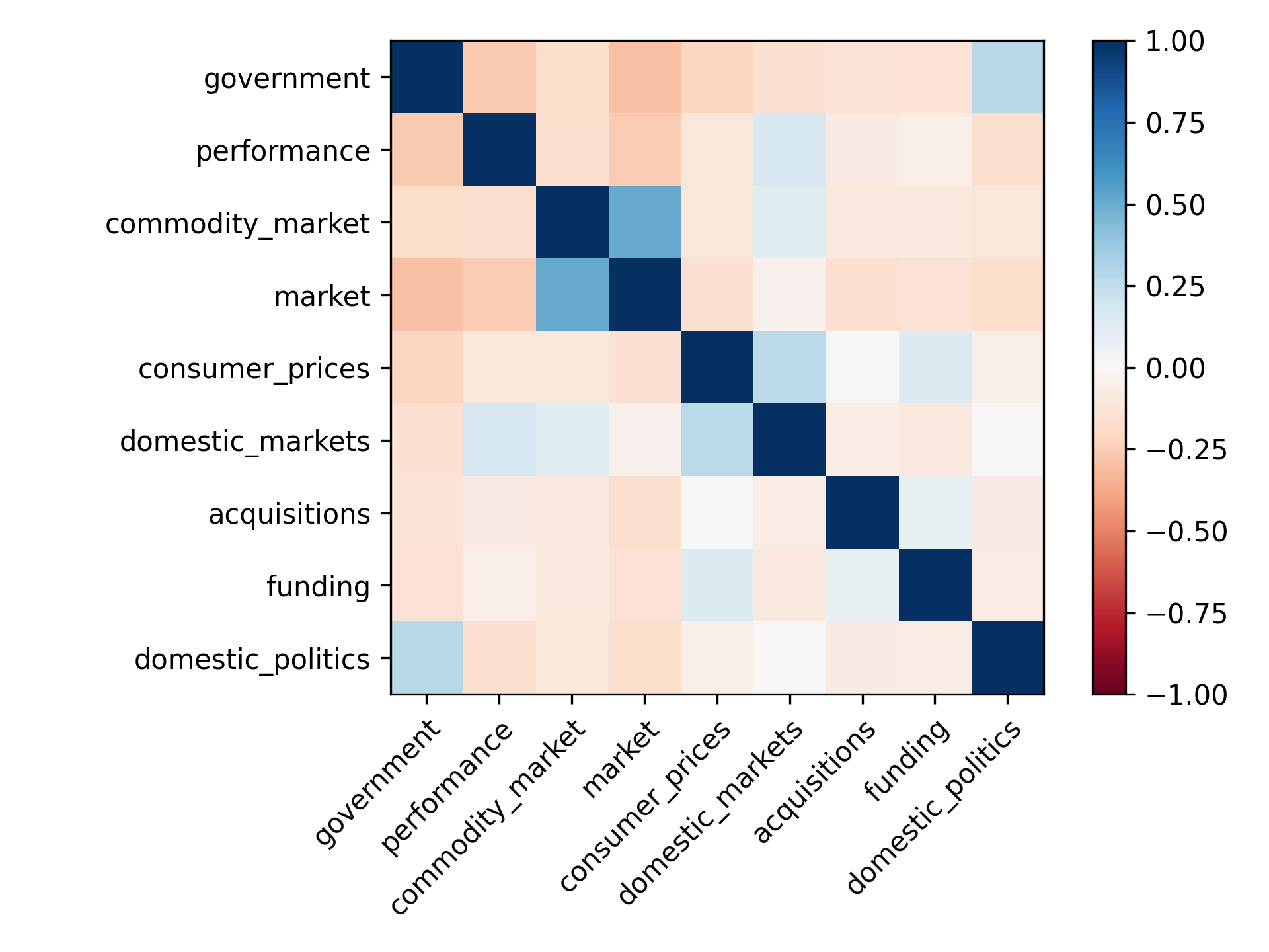
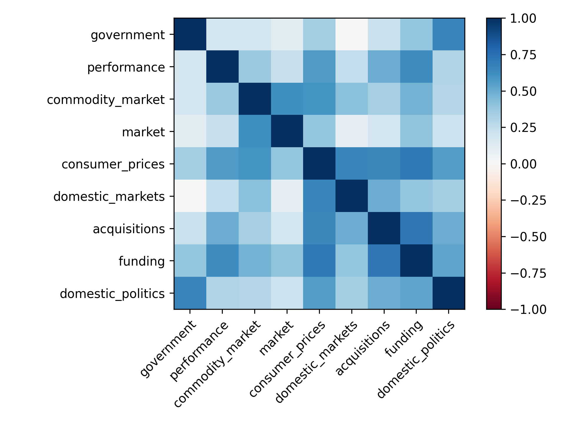
Selected News Topics from RCV1 In RCV1 we select 9 topics to plot heatmaps randomly: government, financial performance, commodity market, consumer prices, domestic markets, acquisitions, funding and domestic politics. Due to the limited space, we only show Pearson correlations and cosine similarities between each pair of our LiGCN model with the best performance in Figure 3. For the Pearson correlation, we could notice that the model captures strong positive relationships between the following pairs: commodity market and market, government and domestic politics, consumer prices and domestic markets. These relationships are consistent with our real life, i.e., government news and domestic political news are very similar. We see a similar trend in the heatmap of cosine similarity for the mentioned label pairs. And in this way, more positive relations are found than negative ones, for example, negative correlation between acquisitions and consumer prices.
6 Conclusion
In this work, we propose a label-interpretable graph model, LiGCN, to solve the MLTC problem as a link prediction task. Our model is able to provide token-level explanation for the classification and therefore enjoys better label interpretability. Experiments on four public datasets show that our model achieved competitive scores. In the future, we will experiment with more complex graph encoders, extend this idea to single-label and extreme multi-label classification tasks Li et al. (2019b).
References
- Bastings et al. (2017) Jasmijn Bastings, Ivan Titov, Wilker Aziz, Diego Marcheggiani, and Khalil Sima’an. 2017. Graph convolutional encoders for syntax-aware neural machine translation. In Proceedings of the 2017 Conference on Empirical Methods in Natural Language Processing, pages 1957–1967, Copenhagen, Denmark. Association for Computational Linguistics.
- Baziotis et al. (2018) Christos Baziotis, Athanasiou Nikolaos, Alexandra Chronopoulou, Athanasia Kolovou, Georgios Paraskevopoulos, Nikolaos Ellinas, Shrikanth Narayanan, and Alexandros Potamianos. 2018. NTUA-SLP at SemEval-2018 task 1: Predicting affective content in tweets with deep attentive RNNs and transfer learning. In Proceedings of The 12th International Workshop on Semantic Evaluation, pages 245–255, New Orleans, Louisiana. Association for Computational Linguistics.
- Chen et al. (2017) G. Chen, D. Ye, Z. Xing, J. Chen, and E. Cambria. 2017. Ensemble application of convolutional and recurrent neural networks for multi-label text categorization. In 2017 International Joint Conference on Neural Networks (IJCNN), pages 2377–2383.
- Deng and Ren (2020) J. Deng and F. Ren. 2020. Multi-label emotion detection via emotion-specified feature extraction and emotion correlation learning. IEEE Transactions on Affective Computing, pages 1–1.
- Devlin et al. (2019) Jacob Devlin, Ming-Wei Chang, Kenton Lee, and Kristina Toutanova. 2019. Bert: Pre-training of deep bidirectional transformers for language understanding.
- Fei et al. (2020) H. Fei, D. Ji, Y. Zhang, and Y. Ren. 2020. Topic-enhanced capsule network for multi-label emotion classification. IEEE/ACM Transactions on Audio, Speech, and Language Processing, 28:1839–1848.
- Feng et al. (2018) Shi Feng, Yaqi Wang, Kaisong Song, Daling Wang, and Ge Yu. 2018. Detecting multiple coexisting emotions in microblogs with convolutional neural networks. Cognitive Computation, 10(1):136–155.
- Ghorbani et al. (2019) Mahsa Ghorbani, Mahdieh Soleymani Baghshah, and Hamid R. Rabiee. 2019. MGCN: semi-supervised classification in multi-layer graphs with graph convolutional networks. In ASONAM ’19: International Conference on Advances in Social Networks Analysis and Mining, Vancouver, British Columbia, Canada, 27-30 August, 2019, pages 208–211. ACM.
- Huang et al. (2019) Chenyang Huang, Amine Trabelsi, and Osmar R Zaïane. 2019. Seq2emo for multi-label emotion classification based on latent variable chains transformation. arXiv preprint arXiv:1911.02147.
- Huang et al. (2020) Lianzhe Huang, Xin Sun, Sujian Li, Linhao Zhang, and Houfeng Wang. 2020. Syntax-aware graph attention network for aspect-level sentiment classification. In Proceedings of the 28th International Conference on Computational Linguistics, pages 799–810, Barcelona, Spain (Online). International Committee on Computational Linguistics.
- Jabreel and Moreno (2019) Mohammed Jabreel and Antonio Moreno. 2019. A deep learning-based approach for multi-label emotion classification in tweets. Applied Sciences, 9(6):1123.
- Kim (2014) Yoon Kim. 2014. Convolutional neural networks for sentence classification. In Proceedings of the 2014 Conference on Empirical Methods in Natural Language Processing (EMNLP), pages 1746–1751, Doha, Qatar. Association for Computational Linguistics.
- Kipf and Welling (2017) Thomas N. Kipf and Max Welling. 2017. Semi-supervised classification with graph convolutional networks. In 5th International Conference on Learning Representations, ICLR 2017, Toulon, France, April 24-26, 2017, Conference Track Proceedings. OpenReview.net.
- Lewis et al. (2004) David D Lewis, Yiming Yang, Tony G Rose, and Fan Li. 2004. Rcv1: A new benchmark collection for text categorization research. Journal of Machine Learning Research, 5:361–397.
- Li et al. (2020a) Irene Li, Alexander Fabbri, Swapnil Hingmire, and Dragomir Radev. 2020a. R-VGAE: Relational-variational graph autoencoder for unsupervised prerequisite chain learning. In Proceedings of the 28th International Conference on Computational Linguistics, pages 1147–1157, Barcelona, Spain (Online). International Committee on Computational Linguistics.
- Li et al. (2019a) Irene Li, Alexander R. Fabbri, Robert R. Tung, and Dragomir R. Radev. 2019a. What should I learn first: Introducing lecturebank for NLP education and prerequisite chain learning. In The Thirty-Third AAAI Conference on Artificial Intelligence, AAAI 2019, The Thirty-First Innovative Applications of Artificial Intelligence Conference, IAAI 2019, The Ninth AAAI Symposium on Educational Advances in Artificial Intelligence, EAAI 2019, Honolulu, Hawaii, USA, January 27 - February 1, 2019, pages 6674–6681. AAAI Press.
- Li et al. (2020b) Irene Li, Yixin Li, Tianxiao Li, Sergio Alvarez-Napagao, Dario Garcia, and Toyotaro Suzumura. 2020b. What are we depressed about when we talk about covid19: Mental health analysis on tweets using natural language processing. arXiv preprint arXiv:2004.10899.
- Li et al. (2019b) Irene Li, Michihiro Yasunaga, Muhammed Yavuz Nuzumlali, Cesar Caraballo, Shiwani Mahajan, Harlan M. Krumholz, and Dragomir R. Radev. 2019b. A neural topic-attention model for medical term abbreviation disambiguation. CoRR, abs/1910.14076.
- Li et al. (2018) Qimai Li, Zhichao Han, and Xiao-Ming Wu. 2018. Deeper insights into graph convolutional networks for semi-supervised learning. In Proceedings of the Thirty-Second AAAI Conference on Artificial Intelligence, (AAAI-18), the 30th innovative Applications of Artificial Intelligence (IAAI-18), and the 8th AAAI Symposium on Educational Advances in Artificial Intelligence (EAAI-18), New Orleans, Louisiana, USA, February 2-7, 2018, pages 3538–3545. AAAI Press.
- Li et al. (2019c) Ran Li, Qingyi Si, Peng Fu, Zheng Lin, Weiping Wang, and Gang Shi. 2019c. A multi-channel neural network for imbalanced emotion recognition. In 2019 IEEE 31st International Conference on Tools with Artificial Intelligence (ICTAI), pages 353–360. IEEE.
- Linmei et al. (2019) Hu Linmei, Tianchi Yang, Chuan Shi, Houye Ji, and Xiaoli Li. 2019. Heterogeneous graph attention networks for semi-supervised short text classification. In Proceedings of the 2019 Conference on Empirical Methods in Natural Language Processing and the 9th International Joint Conference on Natural Language Processing (EMNLP-IJCNLP), pages 4821–4830, Hong Kong, China. Association for Computational Linguistics.
- Liu et al. (2017) Jingzhou Liu, Wei-Cheng Chang, Yuexin Wu, and Yiming Yang. 2017. Deep learning for extreme multi-label text classification. In Proceedings of the 40th International ACM SIGIR Conference on Research and Development in Information Retrieval, Shinjuku, Tokyo, Japan, August 7-11, 2017, pages 115–124. ACM.
- Liu et al. (2019a) Yinhan Liu, Myle Ott, Naman Goyal, Jingfei Du, Mandar Joshi, Danqi Chen, Omer Levy, Mike Lewis, Luke Zettlemoyer, and Veselin Stoyanov. 2019a. Roberta: A robustly optimized BERT pretraining approach. CoRR, abs/1907.11692.
- Liu et al. (2019b) Ziwei Liu, Zhongqi Miao, Xiaohang Zhan, Jiayun Wang, Boqing Gong, and Stella X. Yu. 2019b. Large-scale long-tailed recognition in an open world. In IEEE Conference on Computer Vision and Pattern Recognition, CVPR 2019, Long Beach, CA, USA, June 16-20, 2019, pages 2537–2546. Computer Vision Foundation / IEEE.
- Meyer (2011) Bertrand Meyer. 2011. Towards a calculus of object programs. CoRR, abs/1107.1999.
- Mohammad et al. (2018) Saif Mohammad, Felipe Bravo-Marquez, Mohammad Salameh, and Svetlana Kiritchenko. 2018. SemEval-2018 task 1: Affect in tweets. In Proceedings of The 12th International Workshop on Semantic Evaluation, pages 1–17, New Orleans, Louisiana. Association for Computational Linguistics.
- Nam et al. (2017) Jinseok Nam, Eneldo Loza Mencía, Hyunwoo J. Kim, and Johannes Fürnkranz. 2017. Maximizing subset accuracy with recurrent neural networks in multi-label classification. In Advances in Neural Information Processing Systems 30: Annual Conference on Neural Information Processing Systems 2017, December 4-9, 2017, Long Beach, CA, USA, pages 5413–5423.
- Qi et al. (2018) Hang Qi, Matthew Brown, and David G. Lowe. 2018. Low-shot learning with imprinted weights. In 2018 IEEE Conference on Computer Vision and Pattern Recognition, CVPR 2018, Salt Lake City, UT, USA, June 18-22, 2018, pages 5822–5830. IEEE Computer Society.
- Quan and Ren (2010) Changqin Quan and Fuji Ren. 2010. A blog emotion corpus for emotional expression analysis in chinese. Computer Speech & Language, 24(4):726–749.
- Ragesh et al. (2021) Rahul Ragesh, Sundararajan Sellamanickam, Arun Iyer, Ramakrishna Bairi, and Vijay Lingam. 2021. Hetegcn: heterogeneous graph convolutional networks for text classification. In Proceedings of the 14th ACM International Conference on Web Search and Data Mining, pages 860–868.
- Tang et al. (2015) Duyu Tang, Bing Qin, and Ting Liu. 2015. Document modeling with gated recurrent neural network for sentiment classification. In Proceedings of the 2015 Conference on Empirical Methods in Natural Language Processing, pages 1422–1432, Lisbon, Portugal. Association for Computational Linguistics.
- Tayal et al. (2019) Kshitij Tayal, Rao Nikhil, Saurabh Agarwal, and Karthik Subbian. 2019. Short text classification using graph convolutional network. In NIPS workshop on Graph Representation Learning.
- Wang et al. (2016) Yaqi Wang, Shi Feng, Daling Wang, Ge Yu, and Yifei Zhang. 2016. Multi-label chinese microblog emotion classification via convolutional neural network. In Asia-Pacific Web Conference, pages 567–580. Springer.
- Xiao et al. (2021) Lin Xiao, Xiangliang Zhang, Liping Jing, Chi Huang, and Mingyang Song. 2021. Does head label help for long-tailed multi-label text classification. CoRR, abs/2101.09704.
- Xu et al. (2020) Peng Xu, Zihan Liu, Genta Indra Winata, Zhaojiang Lin, and Pascale Fung. 2020. Emograph: Capturing emotion correlations using graph networks.
- Yang et al. (2018) Pengcheng Yang, Xu Sun, Wei Li, Shuming Ma, Wei Wu, and Houfeng Wang. 2018. SGM: Sequence generation model for multi-label classification. In Proceedings of the 27th International Conference on Computational Linguistics, pages 3915–3926, Santa Fe, New Mexico, USA. Association for Computational Linguistics.
- Yao et al. (2019) Liang Yao, Chengsheng Mao, and Yuan Luo. 2019. Graph convolutional networks for text classification. In Proceedings of the AAAI Conference on Artificial Intelligence, volume 33, pages 7370–7377.
- Zhang et al. (2019) Chen Zhang, Qiuchi Li, and Dawei Song. 2019. Aspect-based sentiment classification with aspect-specific graph convolutional networks. In Proceedings of the 2019 Conference on Empirical Methods in Natural Language Processing and the 9th International Joint Conference on Natural Language Processing (EMNLP-IJCNLP), pages 4568–4578, Hong Kong, China. Association for Computational Linguistics.
- Zhang et al. (2018) Wenjie Zhang, Junchi Yan, Xiangfeng Wang, and Hongyuan Zha. 2018. Deep extreme multi-label learning. In Proceedings of the 2018 ACM on International Conference on Multimedia Retrieval, ICMR 2018, Yokohama, Japan, June 11-14, 2018, pages 100–107. ACM.
- Zhou et al. (2020) Boyan Zhou, Quan Cui, Xiu-Shen Wei, and Zhao-Min Chen. 2020. BBN: bilateral-branch network with cumulative learning for long-tailed visual recognition. In 2020 IEEE/CVF Conference on Computer Vision and Pattern Recognition, CVPR 2020, Seattle, WA, USA, June 13-19, 2020, pages 9716–9725. IEEE.