3D Point Cloud Registration with Multi-Scale Architecture
and Unsupervised Transfer Learning

Abstract

We propose a method for generalizing deep learning for 3D point cloud registration on new, totally different datasets. It is based on two components, MS-SVConv and UDGE. Using Multi-Scale Sparse Voxel Convolution, MS-SVConv is a fast deep neural network that outputs the descriptors from point clouds for 3D registration between two scenes. UDGE is an algorithm for transferring deep networks on unknown datasets in a unsupervised way. The interest of the proposed method appears while using the two components, MS-SVConv and UDGE, together as a whole, which leads to state-of-the-art results on real world registration datasets such as 3DMatch, ETH and TUM. The code is publicly available at https://github.com/humanpose1/MS-SVConv.

1 Introduction

With the increasing number of 3D sensors and 3D data production, the task of consolidating overlapping point clouds, which is called registration, has become a major issue in many applications. Registration can be used online (e.g., in a LiDAR SLAM pipeline for loop closure detection) or offline (e.g., in 3D reconstructions of RGB-D indoor scenes [8] or for outdoor LiDAR map building for autonomous vehicles).

However, point cloud registration can be challenging with real-world scans because of noise, incomplete 3D scan, outliers, and so on. There are numerous existing approaches to this issue; however, recently, deep learning approaches have become very popular, especially for learning descriptors and for computing transformations. These data-driven approaches, especially those that involve learning on large datasets with the ground truth pose as supervision, have been very effective at solving registration problems [53, 13, 19, 18, 3, 4, 14, 11, 9].

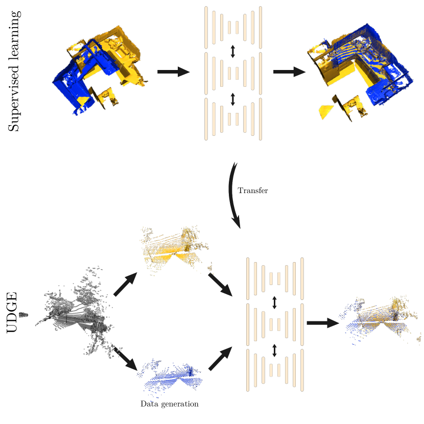
Figure 1: Summary of the proposed method. We can use MS-SVConv for supervised training on a huge dataset, and then we can transfer it in an unsupervised fashion on a smaller dataset.

However, acquiring the ground truth pose can be very costly, and many applications have only small datasets. This is why recent methods are focused on improving the generalization capability of the networks. Therefore, we propose Multi-scale Sparse Voxel Convolution (MS-SVConv), a U-Net-based method to tackle the problem of registration (see Figure 1 for a summary of the proposed method). Using sparse convolutions (such as MinkowskiNet from Choy et al. [11] or SPVNAS from Tang et al. [44]), MS-SVConv is fast and efficient. However, contrary to other U-Net methods, such as FCGF [11], MS-SVConv can compute meaningful descriptors that can generalize with new datasets. Moreover, we also propose Unsupervised transfer learning with Data GEneration (UDGE), so the network can generalize on unknown and small datasets. With this new transfer learning strategy, we show that we can pre-train MS-SVConv on a synthetic dataset, and transfer it to a totally different real-world dataset.

In other words, our contributions are the following:

• We propose a method for generalizing deep learning for 3D point cloud registration on new, totally different datasets, using transfer learning. It is based on two components, MS-SVConv which is a shared multi-scale architecture, and UDGE which is an unsupervised transfer learning using data generation.

• We evaluate the interest of the proposed method on real-world datasets such as 3DMatch, ETH, and TUM datasets. We show that we can pre-train MS-SVConv on a synthetic dataset, and transfer it to a totally different real-world dataset.

MS-SVConv and UDGE, used together as a whole, show the interest of the proposed method.

2 Related works

Many methods have been proposed to tackle rigid point cloud registration. One of the most well-known algorithms is the Iterative Closest Point (ICP) algorithm [5] due to its simplicity, modularity, and effectiveness [38, 17, 6]. Many subsequent variants of the ICP algorithm have been proposed, (e.g., [38, 6]). However, one of the main drawbacks of this algorithm is that it does not work for all initial transformations (the convergence of ICP is local). In addition, the algorithm does not work in every case (when the overlap between two point clouds is too small, or when there are many outliers). Some methods have been proposed to solve the global registration problem (4PCS [1], GoICP [50]). On the other hand, researchers have developed many methods to compute handcrafted descriptors, such as Spin Image [26], SHOT [40], or FPFH [39] on 3D point clouds. Although Hana et al. [22] completed a global review of these descriptors, they do not work well for real-world scans, as excessive noise or occlusion decreases the descriptors’ adaptability.

2.1 Deep learning on 3D point clouds

Unlike images, deep learning on 3D point clouds is challenging because point clouds are unstructured data. Numerous methods have been suggested, such as Multi-View CNN [43] and 3DCNN [31], but these methods require a huge amount of memory. PointNet  [35] and Point-Net++  [36] catalyzed a revolution in deep learning in point clouds and have made possible many new applications  [13, 3, 14, 55]. Recently, many works have tried to generalize convolution for sparse data, such as KPConv [45], Minkowski [10], and RandLaNet [23]. Guo et al. [20] conducted a comprehensive survey of deep learning on 3D point clouds.

2.2 Deep learning for point cloud registration

Recently, registration methods based on deep learning have shown remarkable results on synthetic datasets, such as ModelNet [48], and RGB-D datasets, such as 3DMatch [53]. We observe three trends for these methods:

• The end-to-end methods compute the transformation directly thanks to a fully differentiable framework (such as DCP [46] or PointnetLK [3]).

• Deep descriptors are computed locally on patches (such as 3DSmoothNet [19] or DIP [33]). The transformation is achieved by matching the descriptors.

• Deep descriptors are computed simultaneously on every point through use of an architecture similar to U-Net (such as FCGF [11] or D3Feat [4]). The transformation is also achieved by matching descriptors.

End-to-end methods:

Many end-to-end methods have been proposed to deal with the problem of registration, such as PointNetLK [3], deep closest point [46], DeepVCP [30], RPMnet [51], and PRNet [47]. Some end-to-end methods are also unsupervised [47, 25]. However, most end-to-end methods were tested only on ModelNet, which is a synthetic dataset, and not a real dataset. Actually, Huang et al. [25] tested their method on 7-Scene [41], and the results are promising. However, they have not evaluated their method on 3DMatch dataset. Deep Global Registration [9] is an end-to-end method that performs very well on a real dataset and is built on FCGF [11] but did not demonstrate an ability to generalize efficiently. According to Choy et al. [9], Deep Closest Point [46], and PointNetLK [3] do not work on datasets such as 3DMatch. Recently, PointNetLK has been revisited [29] and has shown promising generalization results on 3DMatch.

Patch-based descriptor matching methods:

Since 3DMatch [53] was introduced, many improvements have been made to the patch-based descriptor matching method. PPFNet [14] uses a PointNet architecture to compute local descriptors, and with global pooling, can compute a global descriptor to bring the global context of the scene. PPF Foldnet [13] and Capsule Net [55] use an autoencoder to compute descriptors without supervision. With 3DSmoothNet [19], great improvements have been made on the 3DMatch dataset [53], and 3DSmoothNet showed great generalization capabilities on the ETH dataset [34]. 3DSmoothNet first computes the local reference frame to orient the patches and then, uses a 3D convolutional neural network on them with a smooth density to compute descriptors. Following the success of 3DSmoothNet, MultiView [28], DIP [33], GeDI [32], and SpinNet [2] also improved upon the generalization capabilities from the 3DMatch dataset [53] to the ETH dataset [34]. But even if these methods are rotation invariant, patch-based methods are very slow in inference. Therefore, in real-world conditions, patch-based methods are inoperable, because of patch extraction. Moreover, because each patch is treated individually, their design is usually not flexible enough to add new capabilities (keypoint detector, end-to-end extension, feature pre-training for semantic segmentation).

U-Net based descriptor matching method:

FCGF [11] is one of the first U-Net methods that was applied to point cloud registration; thanks to the architecture and the sparse voxel convolutions, this method performs very well. It is also much faster than patch-based methods in inference. D3Feat [4] uses Kernel Point convolutions [45] and jointly computes the detector and a descriptor. FCGF and D3Feat show poor generalization capabilities. PREDATOR [24] is composed of a Graph Neural Network and a cross attention module to compute meaningful descriptors, even if the overlap between two scenes is low. These works reveal that U-Net-based methods are more flexible than patch-based methods. They can be coupled easily with a detector or with an end-to-end method [9], and can also be used in multi-scene registration methods [18]. The main problem with these methods is that they have poor generalization capabilities on unknown datasets. The proposed method, which is mainly inspired by FCGF, maintains its advantages (speed, efficiency, modularity) while showing much better generalization capabilities than FCGF.

3 Proposed method

In this section, we describe the following: 1) the problem of registration; 2) the proposed contribution, which uses a multi-scale architecture to improve the U-Net; and 3) the principle of UDGE for unsupervised transfer learning.

3.1 Problem statement

Let $X=(x_{1},\dots x_{N_{X}})\in\mathbb{R}^{N_{X}\times 3}$ and $Y=(y_{1},\dots y_{N_{Y}})\in\mathbb{R}^{N_{Y}\times 3}$ be two point clouds. The goal of registration is to find the right transformation $R\in SO(3),t\in\mathbb{R}^{3}$, which are the sets of 3D rotations and translations. In other words, the goal is to find the set of matches $\mathcal{M}$ and the rotation and translation such that:

$$(R^{*},t^{*},\mathcal{M}^{*})=\operatorname*{arg\,min}_{R\in SO(3),t\in\mathbb{R}^{3}}\sum_{(i,j)\in\mathcal{M}}\|Rx_{i}+t-y_{j}\|^{2}.$$ (1)

Simultaneously, finding the right match and the right transformation is difficult. This problem is divided into two sub-problems. First, we must find correct matches between point clouds, and second, we compute the transformation using a robust estimator, such as RANSAC [15], TEASER [49], or FGR [56]. In our work, we focus on using U-Net based methods to improve the computation of the descriptors. For the robust transformation estimator, we use TEASER [49], because it is faster than RANSAC [15].

U-Net-based methods:

A U-Net architecture can be divided into two parts with an encoder and a decoder; the first part is created by down-sampling the point cloud and computing intermediate features, while the second part is up-sampled and fused with the features computed on the encoder. Thus, a U-Net instantaneously computes descriptors on all points of a point cloud. Let $\psi_{\theta}$ be the U-Net neural network of parameter $\theta$. As input, $\psi_{\theta}$ takes a point cloud (3D coordinates) and input features associated with each point (usually $1$). Therefore, each pair of point clouds $(X\in\mathbb{R}^{N_{X}\times 3},Y\in\mathbb{R}^{N_{Y}\times 3})$ have associated input features ($f^{(in)}_{X}\in\mathbb{R}^{N_{X}\times d_{in}}$ and $f^{(in)}_{Y}\in\mathbb{R}^{N_{Y}\times d_{in}}$, respectively) with $d_{in}$ the dimension of the input feature. We use $\psi_{\theta}$ to compute output features $F_{X}\in\mathbb{R}^{N_{X}\times d},F_{Y}\in\mathbb{R}^{N_{Y}\times d}$:

$$F_{X} =\psi_{\theta}(X,f^{(in)}_{X}),$$ (2)

$$F_{Y} =\psi_{\theta}(Y,f^{(in)}_{Y}),$$ (3)

where $d$ is the output dimension.

With this formulation, we can express many popular architectures for registration (such as FCGF [11] or D3Feat [4]). Then, finding the right output descriptors is a problem of metric learning. We attempt to compute descriptors with minimal distance between positive matches and maximum distance between negatives matches. For each pair of point clouds $(X,Y)$, we minimize the hard negative contrastive loss:

$$L(\theta)= \sum_{(i,j)\in\mathcal{M}^{+}}\{[\|F_{X_{i}}-F_{Y_{j}}\|-m_{+}]_{+}^{2}$$ (4)

$$+\frac{1}{2}[m_{-}-\min_{k|(i,k)\in\mathcal{M}^{-}}\|F_{X_{i}}-F_{Y_{k}}\|]_{+}^{2}$$ (5)

$$+\frac{1}{2}[m_{-}-\min_{k|(k,j)\in\mathcal{M}^{-}}\|F_{X_{k}}-F_{Y_{j}}\|]_{+}^{2}\},$$ (6)

where $[.]_{+}=\max(.,0)$, $\mathcal{M}^{+}$ is the set of positive matches (ground truth matches), and $\mathcal{M}^{-}$ is the set of negative matches. $m+$ is a hyper-parameter called the positive margin, and $m-$ is called the negative margin. We kept $m+=0.1$ and $m-=1.4$ as in FCGF [10].

Although it is also possible to utilize triplet loss, empirically contrastive loss has shown better results [11]. In supervised training, we use the ground truth transformation between pairs of point clouds to obtain positive and negative matches.

Sparse convolution challenges:

When coupled with the RANSAC estimator, FCGF has shown state-of-the-art results on the 3DMatch dataset. This method can handle large point clouds, is memory efficient, and is faster than most deep methods. But when point clouds come from different sensors or a different environment, FCGF cannot generalize (as noted by Bai et al. [4] and Poiesi et al. [33]). FCGF uses sparse voxel convolutions, so has to voxelize the point cloud with a fixed voxel size. Nevertheless, it seems that sparse convolution can overfit on specific sampling. FCGF, because of this, cannot be applied on a dataset where the sampling is different. One solution is to downsample the point cloud, but downsampling leads to a loss of detail and to representations with fewer points. This can impair descriptor matching and lead to points with different densities appearing approximately similar. The problem is we also lose details that could improve descriptor matching. Moreover, it is difficult to fix the side length of the voxel.

3.2 Multi-scale network, MS-SVConv

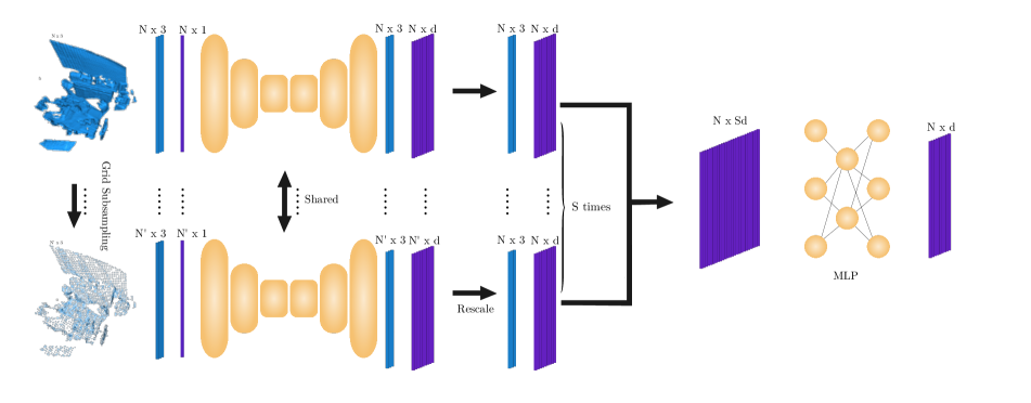
Figure 2: Architecture of the proposed Multi-Scale Sparse Voxel Convolution (MS-SVConv) for registration. The point cloud is downsampled at each scale with a grid subsampling that increases the side length of the voxel by 2 each time.

Downsampled point clouds have a homogeneous density but fewer details, whereas highly dense point clouds contain many details, but also marked variations in density across the scene. Thus, we downsample the point cloud at different scales and then apply the U-Net (we will call it a head) on the downsampled point cloud. Finally, we fuse the features computed by each head using a Multi Layer Perceptron (MLP). An illustration of our multi-scale network is shown in Figure 2. Let $X$ be the input point cloud $X\in\mathbb{R}^{N_{X}\times 3}$ (and the associated input feature $f^{(in)}_{X}\in\mathbb{R}^{N_{X}\times d_{in}}$). Let $s$ be a scale and $\psi_{\theta}^{(s)}$ a U-Net operating at the scale $s$ with the parameter $\theta$:

$$\small F_{X}=MLP(\bigoplus_{s=1}^{S}\psi_{\theta}^{(s)}(X,f^{(in)}_{X})),$$ (7)

where $\bigoplus$ means concatenation. We apply the same MLP for each output of the U-Net.
The MLP will learn to select and filter outputs of each scale. As input, we voxelize the point cloud by increasing the side length of the voxel by two at each scale (performing a grid subsampling). The number of occupied voxels will then be different for each U-Net. We assign the same output descriptor for all points of the original point cloud that fall into the same voxel at a specific scale (called Rescale in Figure 2).

In the U-Net architecture, there are multiple downsampling operations that increase the receptive field. However, a classical U-Net for a 3D point cloud with three layers of downsampling brings a receptive field of eight times the side length of the initial voxel. By using three scales of point clouds, we are able to multiply the side length of the initial voxel by 64, bringing more global contexts to computation of the descriptors.

We use the same network for the different scales with shared weights: this means that we keep the same number of parameters as for one U-Net scale and add only the additional parameters of the final MLP.

Prior works have investigated multi-scale architectures in 3D, but in different ways and contexts. Mu-net [27] is an unshared sequential U-Net on dense voxel grid for denoising. This method is different from our parallel shared multi-scale U-Net with sparse convolution. MS-DeepVoxScene [37] takes several neighborhoods (scales) as input to classify only one point, and is used for semantic segmentation of point clouds. However, in our case, we take the whole point cloud sub-sampled at different scales. The multi-scale network both improves the descriptors in supervised learning, and the capacity of U-Net architectures to generalize.

3.3 Unsupervised transfer learning with UDGE

A supervised setting includes pairs of point clouds and the relative pose between them. The two points clouds are different because they come from different points of view of the scene. The principle of Unsupervised transfer learning with Data GEneration (UDGE) is to use specific data generation to create two partial point clouds from one point cloud. We randomly crop the original data and then apply periodic sampling to simulate partially overlapping views from one scene. This method allows to generate two point clouds, while knowing perfectly the positive and negative matches. In the proposed method, we train in a supervised fashion on a source dataset $S$ and then use UDGE on a target dataset $T$ by using, as initialization, weights trained on $S$. We do not need the ground truth poses on target dataset $T$, and we will show improvements after transfer learning, even if the target dataset $T$ is small. The work closest to UDGE is from [52], but the authors performed self-supervision without pre-training. We show that without pre-training, self-supervision can work for large datasets but not at all for small datasets. Additionally, the author used only one point cloud as a pair, while we utilize specific procedures, like cropping and periodic sampling, to create two partially overlapping point clouds.

Our data generation:

Figure 3 shows how data is generated from one original scan. We distinguish between data generation and data augmentation. Data generation concerns the proposed process of making two partial scans from a point cloud. Thus, the goal of data generation is to generate, without supervision, new data from a point cloud that is in the same case as data from supervised learning. The data generation parameters depend on the target dataset. In contrast, data augmentation is used to artificially increase the size of the dataset. In our case, we also perform data augmentation with the two scans, in particular the classical data augmentation in point clouds that are random rotation around all axes, random scale and noise (jitter). Data generation is already used on ModelNet to simulate partial views of an object, but it is mainly used to test methods on partial scans (see [51], for example). It is not used for training. In our case, we apply our strategy on real unknown datasets from RGB-D frames or LiDAR scans. Although a similar work is undertaken in [54], they performed self-supervision only for pre-training for semantic segmentation. In the case of UDGE, we use data generation for unsupervised transfer learning for point cloud registration and not as pre-training.

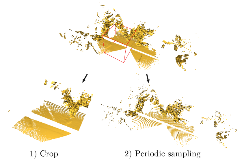
Figure 3: The two data generation methods we use in our unsupervised transfer learning.

Crop:

Similar to images, it is possible to select a local zone of the point cloud and learn from it. To accomplish this, we select a random point and a random 3D shape (it can be a cube or a sphere). Points inside the shape are kept, and points outside the shape are discarded. Selecting a local zone is very useful for simulating pairs of partially overlapping point clouds.

Periodic sampling:

Real scans do not necessarily have regular sampling because sampling depends on the point of view. We propose a data generation technique to simulate irregular sampling that is called periodic sampling (see in Figure 3). The principle is to remove points periodically with respect to a center chosen randomly. Let $c\in\mathbb{R}^{3}$ be a random center. We can compute the mask $M\in\{0,1\}^{N}$of the point cloud $X\in\mathbb{R}^{N\times 3}$. $m_{i}$ is a binary value that indicates whether we keep $x_{i}$ or not. The proposed mask is:

$$\small m_{i}=\mathbf{1}(|\cos(\frac{2\pi}{T}\|x_{i}-c\|)|>\cos(\alpha\pi)),$$ (8)

where $\alpha\in[0,1]$ is a threshold that indicates the proportion of points we want to keep. If $\alpha=0$, every point is removed, and if $\alpha=1$, we keep every point. $T$ is the periodic sampling period. By changing the period $T$ and the threshold $\alpha$, we can simulate a wide range of different types of sampling. Periodic sampling is especially useful for scenes, where sampling is highly irregular.

4 Experiments

We evaluate our contributions on the 3DMatch [53], ETH [34] and TUM [42] datasets. We first describe the datasets used for the experiments, and we show the impact of the multi-scale architecture on supervised learning. Finally, we show the results for generalization of MS-SVConv thanks to multi-scale architecture and UDGE. The implementation details and more experiments on MS-SVConv and UDGE can be found in the supplementary material.

4.1 Datasets

ModelNet [48] (source dataset):

ModelNet40 [48] is a CAD dataset containing around 10,000 objects with 40 object categories. This dataset is used for classification, but many deep learning methods use it for point cloud registration [47, 3, 46]. We use the training set of ModelNet40 for pre-training. Our goal is to show that we can train on a synthetic dataset, such as ModelNet [48], and can generalize on a real-world dataset, such as the ETH dataset.

3DMatch [53] (source and target dataset):

3DMatch [53] is a dataset composed of RGB-D frames from different indoor datasets related to 3D reconstruction, such as BundleFusion [12], SUN3D [21], or 7-Scene [41]. The dataset consists of 62 scenes, and as in [11], we split the dataset into training with 48 scenes, validation with 6 scenes, and a test set of 8 scenes. To create point clouds, we must first process the depth frames; to generate these point clouds, we use TSDF fusion from 50 depth images [14, 11, 4, 19]. The test set is provided by the 3DMatch website. 3DMatch [53] is used for supervised training (pairs of fragments with 30% overlap as in [19]). We also use 3DMatch as the target dataset for UDGE with pre-training on ModelNet.

ETH Dataset [34] (target dataset):

The ETH dataset [34] is an outdoor and indoor 3D point cloud dataset acquired with a 2D LiDAR: it is composed of eight scenes, six outdoors and two indoors. This dataset is considered to be difficult to work with because of complications related to noise and irregular density. We will make a difference between the ETH 8-scenes, following the rigorous protocol described by Fontana et al. [16] and the ETH 4-scenes, following the Gojcic et al.’s benchmark [19] and mainly followed in previous published works such as [4, 2, 33, 19, 32].

TUM dataset [42] (target dataset):

TUM is a RGB-D dataset [42] mainly used for RGB-D SLAM or odometry. We use a single frame as point cloud, following the protocol of Fontana et al. [16]. This dataset is also used to evaluate the proposed unsupervised transfer learning method.

4.2 Metrics

To evaluate the method, we use two metrics: the Feature Match Recall (FMR) and the Scaled Registration Error (SRE).

Let $(X_{i},Y_{i})$ be a pair of scenes. We call $\mathcal{M}(X_{i},Y_{i})$ the matches between $X_{i}$ and $Y_{i}$, $|\mathcal{M}|$ the number of matches, and $(R^{(gt)},t^{(gt)})$ the ground truth rotation and translation. The hit ratio is:

$$\small H(X_{i},Y_{i})=\frac{1}{|\mathcal{M}|}\sum_{k,l\in\mathcal{M}(X_{i},Y_{i})}\mathbf{1}(\|R^{(gt)}x_{k}+t^{(gt)}-y_{l}\|\leq\tau_{1}).$$ (9)

The Feature Match Recall (FMR) is then defined as

$$\small\text{FMR}=\frac{1}{N}\sum_{i=1}^{N}\mathbf{1}(H(X_{i},Y_{i})\geq\tau_{2}),$$ (10)

where $N$ is the number of pairs of scenes. As in previous works [19, 4, 11, 33], we assign $\tau_{1}=0.1$ m and $\tau_{2}=0.05$ by default. Similar to [19, 4, 2, 33, 28], we perform a symmetric test to filter the matches before evaluation. This metric allows evaluating descriptor matching. Although it is useful for comparison of different descriptor-matching methods, we cannot use it to compare different registration algorithms (and therefore, we cannot use it to evaluate classical registration algorithms, such as ICP). To measure the registration error, we use the error defined by Fontana et al. [16]. We call it the Scaled Registration Error (SRE). Suppose we have a point cloud $X\in\mathbb{R}^{N_{X}\times 3}$ and $(R^{(gt)},t^{(gt)})$ is the ground truth transformation between $X$ and $Y$. We want to evaluate our algorithm, which produces the transformation $(R^{*},t^{*})$. The SRE for a pair X, Y is defined as:

$$SRE(X,Y) =\frac{1}{N_{X}}\sum_{i=1}^{N_{X}}\frac{\|(R^{(gt)}x_{i}+t^{(gt)})-(R^{*}x_{i}+t^{*})\|}{\|(R^{(gt)}x_{i}+t^{(gt)})-(R^{(gt)}\bar{x}+t^{(gt)})\|}$$ (11)

$$\bar{x} =\frac{1}{N_{X}}\sum_{i=1}^{N_{X}}x_{i}.$$ (12)

The SRE depends on X and Y, because we estimate $R^{*}$ and $t^{*}$ from $X$ and $Y$. For every pair of scans in a dataset with $N$ pairs, we compute the median of the SRE:

$$SRE=\text{median}_{i=1\dots N}(SRE(X_{i},Y_{i})).$$ (13)

The mean is sensitive to outlier results and is not representative of the results, as explained in [16].

4.3 Evaluation of supervised learning

Supervised learning on 3DMatch
	FMR (%)	FMR (%)
Methods	$\tau_{2}=0.05$	$\tau_{2}=0.2$
SHOT [40]	23.8	-
FPFH [39]	35.9	-
3DMatch [53]	59.6	-
PPFNet [14]	62.3	-
3DSmoothNet [19]	94.7	72.9
DIP [33]	94.8	-
FCGF [11]	95.2	67.4
FCGF∗ [11]	97.5	87.3
D3Feat [4]	95.8	75.8
Multiview [28]	97.5	86.9
SpinNet [2]	97.6	85.7
Predator [24]	96.6	-
GeDI [32]	97.9	-
MS-SVConv (1 head)	97.6	87.2
MS-SVConv (3 heads)	98.4	89.9

Table 1: Feature Match Recall (FMR) on 3DMatch for two hit ratio parameters $\tau_{2}$. Results from published methods are taken from the papers. FCGF^∗ means that we evaluate ourselves the original code with a symmetric test, before computing the FMR.

We evaluate the impact of MS-SVConv on supervised learning to see the influence of the multi-scale architecture. Table 1 shows the results on 3DMatch. Although the 3DMatch benchmark is very competitive, MS-SVConv outperforms all published methods. If we compare MS-SVConv with the best published method (MultiView [28]), we have an augmentation of +3% on the Feature Match Recall (FMR) with $\tau_{2}=0.2$. Table 1 shows that MS-SVConv with three heads is much better than with a single head (a single scale), which demonstrates the interest of multi-scale methods for supervised learning. MS-SVConv with one head and FCGF are conceptually similar but MS-SVConv has a different implementation, see supplementary material. Moreover, contrary to other methods, FCGF does not filter matches with a symmetric test. If we filter matches with a symmetric test, results of FCGF and MS-SVConv with one head are similar (see Table  1).

4.4 Evaluation of UDGE

Unsupervised learning on ETH dataset
	ETH	ETH
	4-scenes	8-scenes
Methods	FMR (%)	FMR (%)	SRE	Time (s)
Classical method
FPFH [39]	22.1	0.75	85.1	0.71
Patch based deep methods without UDGE
3DSmoothNet [19]	79.0	-	-	-
Multiview [28]	92.3	42.6	44.0	56.0
DIP [33]	92.8	93.9	6.9	8.27
GeDI [32]	98.2	-	-	-
U-Net based deep methods without UDGE
D3Feat [4]	61.6	64.5	95.0	0.43
MS-SVConv(1)	34.9	56.4	151.0	0.24
MS-SVConv(3)	71.8	76.8	82.2	0.52
U-Net based deep methods with UDGE
MS-SVConv(1)	88.0	87.5	44.0	0.16
MS-SVConv(3)	98.9	93.6	6.9	0.40

Table 2: Feature Match Recall (FMR) and median Scaled Registration Error (SRE) x1000 on the ETH dataset with deep methods trained on 3DMatch. ETH 4-scenes follows Gojcic et al.’s benchmark [19], and results from other methods are published results (only FMR available). ETH 8-scenes follows Fontana et al. [16] protocol, and all methods are computed using codes available online (FMR, SRE, and Time). MS-SVConv(1) means MS-SVConv with one head; MS-SVConv(3) means MS-SVConv with three heads. We report only the average time of descriptor extraction.

Table 2 shows the results on the ETH dataset [34] with and without UDGE after pre-training on 3DMatch. ETH is a challenging dataset because of the density variation and missing areas. Without UDGE, MS-SVConv with one head has average results on ETH of only 34.9% on the ETH 4-scenes and 56.4% FMR on ETH 8-scenes. MS-SVConv with three heads has +36.9% FMR on ETH 4-scenes and +20.4% FMR improvement on ETH 8-scenes without UDGE, thanks to the multi-scale architecture. This demonstrates the capability of multi-scale architecture to improve the generalization capacity of U-Net, and proves useful for registration in online settings.

With UDGE, MS-SVConv(3) gets state-of-the-art results with 98.9% FMR on ETH 4-scenes and 93.6% FMR on ETH 8-scenes like the best patch-based method DIP [33] while 20 times faster. There is a synergy between multi-scale and UDGE, with +10.9% and +6.1% improvement of the FMR between one and three heads.

Adding heads increase the generalization capability, but the training time and the inference time are multiplied by 2.5 (from 0.16 s to 0.40 s for the average time of descriptor extraction). Nonetheless, the proposed network is still much faster than any other deep method we tested.

Unsupervised learning on ETH dataset
	Scenes used for UDGE				Scenes for testing
Methods	Haupt.	Stairs	Plain	Apart.	Gaz. Sum.	Gaz. Wint.	Wood Aut.	Wood Sum.	Average
MS-SVConv(1)	53	93	76	100	85	99	84	89	84.9
MS-SVConv(3)	72	99	88	100	96	100	99	99	94.1

Table 3: Feature Match Recall (FMR) with $\tau_{2}=0.05$ per scene on the ETH 8-scenes dataset [16]. MS-SVConv was pre-trained on ModelNet, and data generation for UDGE comes only from Hauptgebaude, Stairs, Plain and Apartment.

Influence of the source dataset $S$:

Unsupervised learning on ETH dataset
	FMR (%)	FMR (%)
Source	(without UDGE)	(with UDGE)
ModelNet	74.1	93.4
3DMatch	76.8	93.6

Table 4: Influence of source dataset $S$ for the target ETH 8-scenes dataset with MS-SVConv(3).

Surprisingly, thanks to the proposed multi-scale architecture and the data generation for transfer learning, ModelNet pre-training (48 h instead of three weeks for training on 3DMatch) is enough to obtain very good results with the ETH dataset (see Table 4). This shows that even if the source dataset and the target dataset are very different, MS-SVConv will still work.

	Target	ETH	TUM	3DMatch
Source
$\emptyset$		0.0	16.0	60.3
ModelNet		93.4	100	96.5
3DMatch		93.6	99.7	97.8

Table 5: UDGE on the ETH, TUM, and 3DMatch datasets with no pre-training ($\emptyset$) or with pre-training on ModelNet or pre-training on 3DMatch. The results are Feature Match Recall in % with MS-SVConv(3).

Pre-training in a supervised fashion is essential. We can see in Table 5 that, with no pre-training, UDGE’s results are very poor, especially on small datasets like ETH and TUM. Decent results (60.3% FMR) are still produced when the dataset is much larger like 3DMatch. However, supervised pre-training on ModelNet is enough to have state-of-the-art results thanks to UDGE and without any ground truth for any of the target datasets (ETH, TUM, or 3DMatch). It shows that UDGE can bring good results even if the target dataset is small.

Does UDGE allow for generalization on unseen scenes?

In all experiments, UDGE involves taking the test set and artificially creating point cloud pairs to fit the network to the new dataset. Even if we use the test set for the transfer, the proposed protocol is valid because UDGE does not use the ground truth poses of the test set. But to what extent will the transfered descriptors generalize on unseen scenes? To see if the results remain similar, we split the ETH dataset in two: After pre-training on ModelNet, we apply UDGE on MS-SVConv with four scenes from ETH dataset (Plain, Stairs, Hauptgebaude and Apartment) and we evaluate it on the four others (Gazebo Summer, Gazebo Winter, Wood Autumn, and Wood Summer). We use the same hyper-parameters as in the previous training (see the section Implementation Details in supplementary material), except that the number of epochs is 400 instead of 200. Table 3 shows that even if MS-SVConv has never seen Gazebo and Wood, the method can still generalize on these scenes.

Influence of the proposed data generation:

Crop	Periodic Sampling	FMR (%)
		88.4
✓		91.4
✓	✓	93.4

Table 6: Influence of the proposed data generation in UDGE: MS-SVConv(3) is pre-trained on ModelNet and UDGE is applied on the ETH 8-scenes dataset.

We performed experiments on the ETH dataset to see the influence of the proposed data generation of UDGE. After pre-training MS-SVConv(3) on ModelNet, we tried UDGE on the ETH dataset without cropping or using periodic sampling (using the same point cloud for pairs as in [52]). Table 6 shows that cropping is important in data generation. If we do not perform this operation, the performance drops from 91.4% to 88.4% on the FMR. Periodic sampling also brings improvements. This experiment highlights that the data generation method in UDGE improves the registration results.

5 Conclusion

We presented MS-SVConv, a multi-scale U-Net based method for descriptor matching in point cloud registration. We also presented UDGE, a simple yet efficient method for generalizing on unknown scenes. The multi-scale architecture leads to gain state-of-the-art results on 3DMatch for supervised learning. With UDGE, it is possible to transfer descriptors for registration on an unknown dataset without any supervision. Additionally, simply by pre-training on a synthetic dataset like ModelNet, we obtain state-of-the-art results on the ETH, TUM, and 3DMatch datasets with UDGE. In contrast to patch-based methods, MS-SVConv retains the simplicity, speed, efficiency, and modularity of U-Net-based methods.

Acknowledgments

This work was granted under the funding of the Idex PSL with the reference ANR-10-IDEX-0001-02 PSL. This work was granted access to the HPC resources of IDRIS under the allocation 2020-AD011012181 made by GENCI.

Supplementary material: 3D Point Cloud Registration with Multi-Scale Architecture and Unsupervised Transfer Learning Sofiane Horache Jean-Emmanuel Deschaud François Goulette
MINES ParisTech, PSL University, Centre for Robotics, 75006 Paris, France
firstname.surname@mines-paristech.fr
We present additional analysis of the method presented in the main article with justifications of the design choices (hyper-parameters of the U-Net network, influence of the number of heads, importance of shared weights) as well as a more in-depth analysis of the results on the 3DMatch and ETH datasets. The first section describes the experiments on MS-SVConv, and the multi-scale architecture in the supervised case. The second section focuses on experiments on UDGE, and the synergy between UDGE and MS-SVConv. The third section specifies implementation and protocol details. Finally, we show qualitative results on the last section (with images) of the registration on the 3DMatch, the ETH, and the TUM datasets.

Appendix A More experiments on supervised learning with MS-SVConv

In this section, we present more experiments to show that MS-SVConv with three heads has great generalization capabilities in comparison with MS-SVConv with one head. We show that a simple pre-training on ModelNet can bring significant results. We also present an experiment to show that MS-SVConv is robust to random rotations. We also show that even if the number of interest points for the matching is low, MS-SVConv have great results on the 3DMatch dataset. Finally, we show that MS-SVConv works very well on scenes with low overlap. The last subsection shows details of results of the 3DMatch dataset

A.1 Generalization capability of MS-SVConv without UDGE

	Target	ETH	TUM	3DMatch
Architecture
MS-SVConv(1)		56.4	99.0	97.6
MS-SVConv(3)		76.8	100	98.4

Table 7: Feature Match Recall ($\tau_{2}=0.05$) of MS-SVConv trained on the 3DMatch dataset with a voxel size of 2 cm and evaluated on ETH 8-scenes, TUM and 3DMatch without UDGE.

	Target	ETH	TUM	3DMatch
Architecture
MS-SVConv(1)		37.4	28.3	29.2
MS-SVConv(3)		74.1	99.3	85.0

Table 8: Feature Match Recall ($\tau_{2}=0.05$) of MS-SVConv trained on the ModelNet dataset with a voxel size of 2 cm and evaluated on ETH 8-scenes, TUM and 3DMatch without UDGE.

Table 7 shows the Feature Match Recall without UDGE on ETH 8-senes, TUM and 3DMatch datasets after having trained our models on the 3DMatch dataset (Table 8 when we train on the ModelNet dataset). These tables show that multi-scale improves generalization capabilities. Moreover, when the training set is the ModelNet dataset, Table 8 shows that multi-scale brings huge improvement (up to +71%) between MS-SVConv with three heads and our U-Net with one head. With the proposed multi-scale sparse voxel convolutions, ModelNet as a pre-training set is enough to compute meaningful descriptors.

A.2 Robustness to random rotations

		w/o Rotation	w Rotation
Architecture
MS-SVConv(1)		87.2	87.0
MS-SVConv(3)		89.9	89.7

Table 9: Feature Match Recall on 3DMatch ($\tau_{2}=0.2$) in supervised learning with and without random rotations in the test set.

U-Net based methods with sparse voxel convolutions are often considered non-robust to random rotations. It is true that they are not invariant by rotation by design, but become robust thanks to data augmentation. In all of our training, we added data augmentation with random rotations in all directions. To test the final robustness, we added large random rotations in the 3DMatch test set. Table 9 shows that the results are almost equivalent on the 3DMatch dataset with or without rotation.

A.3 Influence of the number of points

For all the previous experiments on the 3DMatch and the ETH dataset, we sample randomly 5000 points before matching. To show that MS-SVConv computes meaningful descriptors for each points, we tried to sample different number of points. Table 10 shows that even if we sample 250 points, we have a FMR of 96.3 so a loss of 2.1%. Except the patch-based mathod GeDI, all other methods have a more significant drop of result when the number of point decreases. It shows that MS-SVConv computes more meaningful descriptors at each points, thanks to the multi-scale computation that brings more contexts.

Number of points	5000	2500	1000	500	250	Av.
Perfect Match [19]	94.7	94.2	92.6	90.1	82.9	90.9
FCGF [11]	95.2	95.5	94.6	93.0	89.9	93.6
D3Feat(rand) [4]	95.3	95.1	94.2	93.6	90.8	93.8
D3Feat(pred) [4]	95.8	95.6	94.6	94.3	93.3	94.7
SpinNet [2]	97.6	97.5	97.3	96.3	94.3	96.6
GeDI [32]	97.9	97.7	97.6	97.2	97.3	97.5
MS-SVConv(3)	98.4	97.9	97.0	97.9	96.3	97.5

Table 10: Influence of the number of points for supervised learning on the 3DMatch dataset (FMR with $\tau_{2}=0.05$).

A.4 Results on the 3DLoMatch dataset

3DLoMatch [24] is a dataset containing the previously ignored scan pairs of 3DMatch that have low 10-30% overlap. We compare MS-SVConv with Predator [24] on the 3DMatch and 3DLoMatch dataset. Predator is a very sophisticated method that use graph convolutional neural network and deep attention module after the encoder to compute meaningful descriptors even when the overlap is very low. On the contrary, MS-SVConv uses a simple multi-scale architecture. We compare MS-SVConv(3) on 3DMatch and 3DLoMatch. Table 11 shows that MS-SVConv outperforms Predator on 3DMatch and 3DLoMatch (please, note that contrary to Predator, MS-SVConv does not use a detector to select keypoints, but take random points).

	3DMatch	3DLoMatch
Predator [24]	96.6	73.0
MS-SVConv(3)	98.4	77.2

Table 11: Comparison between Predator [24] and MS-SVConv(3) on the 3DMatch and 3DLoMatch dataset in supervised learning. Results are Feature Match Recall (FMR) in %.

A.5 3DMatch results details

We present in Table 12 and Table 13 the details of results of 3DMatch in supervised learning for the different scenes of the dataset with $\tau_{2}=0.05$ and $\tau_{2}=0.2$.

Methods	Kitchen	Home 1	Home 2	Hotel 1	Hotel 2	Hotel 3	Study	MIT Lab	Average
3DSmoothNet [19]	97.0	95.5	89.4	96.5	93.3	98.2	94.5	93.5	94.7
FCGF [11]	-	-	-	-	-	-	-	-	95.2
FCGF∗ [11]	99.0	99.4	91.8	98.2	97.1	98.1	96.6	100.0	97.5
D3Feat [4]	-	-	-	-	-	-	-	-	95.8
MultiView [28]	99.4	98.7	94.7	99.6	100	100	95.5	92.2	97.5
SpinNet [2]	99.2	98.1	96.1	99.6	97.1	100	95.6	94.8	97.6
DIP [33]	-	-	-	-	-	-	-	-	94.8
GeDI [32]	-	-	-	-	-	-	-	-	97.9
MS-SVConv(1)	98.8	98.1	92.8	99.6	99.0	100	96.6	96.1	97.6
MS-SVConv(3)	99.6	99.4	94.2	99.1	99.0	100	95.9	100	98.4

Table 12: Feature Match Recall with $\tau_{2}=0.05$ on 3DMatch in supervised learning. FCGF^∗ means that we evaluate ourselves the original code with a symmetric test, before computing the FMR.

Methods	Kitchen	Home 1	Home 2	Hotel 1	Hotel 2	Hotel 3	Study	MIT Lab	Average
3DSmoothNet [19]	62.8	76.9	66.3	78.8	72.1	88.9	72.3	64.9	72.9
FCGF [11]	-	-	-	-	-	-	-	-	67.4
FCGF∗ [11]	91.1	91.7	78.4	94.2	90.4	90.7	85.3	76.6	87.3
D3Feat [4]	-	-	-	-	-	-	-	-	75.8
MultiView [28]	89.5	85.9	81.3	95.1	92.3	94.4	80.1	76.6	86.9
SpinNet [2]	-	-	-	-	-	-	-	-	85.7
DIP [33]	-	-	-	-	-	-	-	-	-
GeDI [32]	-	-	-	-	-	-	-	-	-
MS-SVConv(1)	88.7	89.1	82.7	95.1	91.3	90.7	83.6	76.6	87.2
MS-SVConv(3)	95.8	94.2	83.7	95.6	88.5	88.9	87.0	85.7	89.9

Table 13: Feature Match Recall with $\tau_{2}=0.2$ on 3DMatch in supervised learning. FCGF^∗ means that we evaluate ourselves the original code with a symmetric test, before computing the FMR.

Appendix B More experiments on the synergy between UDGE and MS-SVConv

In this section, we present experiments on UDGE. We show that shared U-Net is better than unshared U-Net. In addition, we explain why we choose three U-Net for MS-SVConv. We show that three heads is a good trade-off between good generalization and computation. We also present an experiment to show that UDGE can be used for 100% unsupervised training on the 3DMatch dataset. This results suggest that when the dataset is huge and the ground truth is not available, UDGE can be used to learn meaningfull features in an unsupervised fashion. We explain how we can choose the voxel size with UDGE and how we choose the size of crop. We show that for different voxel size, the results do not change a lot. However, for the size of crop, it is quite important and must be well chosen. Finally, we show details results on the ETH dataset.

B.1 To share or not to share?

ETH 8-scenes Dataset
Methods	FMR (%)	SRE	Time (s)
Without UDGE
MS-SVConv(1)	56.4	151.0	0.24
MS-SVConv(3) Unshared	67.4	129.6	0.50
MS-SVConv(3)	76.8	82.2	0.52
With UDGE
MS-SVConv(1)	87.5	44.0	0.16
MS-SVConv(3) Unshared	93.5	33.1	0.335
MS-SVConv(3)	93.6	6.9	0.40

Table 14: Feature Match Recall (FMR) and median Scaled Registration Error (SRE) x1000 on ETH 8-scenes dataset with network pre-trained on 3DMatch. MS-SVConv(1) means MS-SVConv with 1 head and MS-SVConv(3) means MS-SVConv with 3 heads. Unshared means a multi-scale network with different weights at each scale. We only report the average time of descriptor extraction.

We compare the results of the multi-scale by having shared weights or not between the U-Net. Table 14 shows that when we do not share weights (i.e. three different U-Net for the three heads), we see that the generalization capacity results are much lower than the multi-scale with shared weights. Indeed, the gain is only +11% with the unshared weights while it is +20.4% on the Feature Match Recall for the shared weights during the transfer from the 3DMatch to ETH datasets. One reason for this may come from the fact that with unshared weights, each head specializes on a scale while the same network shared between scales learns to be robust to the notion of scale and will adapt better to a new dataset. As in multi-task learning, weights can be beneficial for every scale. We can notice that with UDGE, results are quite similar between shared and unshared networks (as it was the case for fine-tuning with two, three or four heads), but MS-SVConv with three shared heads still obtains better results. This experiment results explain why we choose shared U-net.

B.2 Influence of the number of heads

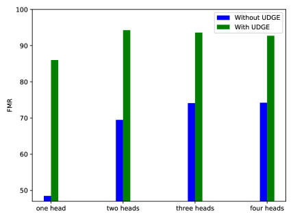
Figure 4: Feature Match Recall (FMR) on ETH 8-scenes dataset in function of the number of head without and with UDGE (model pre-trained on the ModelNet dataset).

The different experiments on the the 3DMatch and the ETH dataset have shown the superiority of the proposed multi-scale network with three heads compared to one head in supervised training, for transfer after using UDGE. But how do we fix the number of heads? To answer this question, we train several networks on the ModelNet dataset with different number of heads and we compute the FMR on the ETH 8-scenes dataset without UDGE and with UDGE. As in previous experiments, the voxel size on the ETH dataset is set at 2 cm with no UDGE and 4 cm with UDGE (the length side of the voxels at the next scale is always 2 times that of the previous scale). Figure 4 shows the FMR in function of the number of head. These results show that the more heads we add, the more the network is able to generalize (without UDGE) between the ModelNet, and the ETH dataset (results slightly decreases with 4 heads). With UDGE, we see that two heads is already enough to achieve excellent descriptor registration performance on ETH. Thus, three heads is a good trade-off to have a very good capacity for generalization on new datasets while having excellent performance with UDGE but keeping a sufficiently fast processing time (2.5 times slower between 3 heads and one head).

B.3 100% unsupervised training on 3DMatch with UDGE

To show that our method can adapt to unseen scenes, and be applied in an unsupervised way, we realized an other experiment with the 3DMatch dataset. We first pre-train on the ModelNet dataset and then apply our unsupervised transfer learning strategy UDGE on the training set of the 3DMatch dataset. We finally evaluate MS-SVConv on the test set of the 3DMatch dataset. Results in Table 15 show that MS-SVConv trained in an unsupervised fashion is very close to supervised learning and comparable to other state-of-the-art methods, while being only trained on the synthetic dataset ModelNet. This is a second experiment which shows that the proposed method UDGE is not just over-fitting on the training set.

Method	FMR ($\tau_{2}=0.05$)	FMR ($\tau_{2}=0.2$)
Supervised	98.4	89.9
UDGE	96.7	85.0

Table 15: Comparison between supervised learning and unsupervised learning on 3DMatch. For unsupervised: model pre-trained on ModelNet and using UDGE on training set of 3DMatch (i.e. not using ground truth poses of 3DMatch). Model is MS-SVConv(3) for supervised and unsupervised results.

B.4 Influence of voxel side length for UDGE

Voxel size (cm)	2	4	6
MS-SVConv(1)	67.3	87.5	91
Voxel size (cm)	2, 4, 8	4, 8, 16	6, 12, 24
MS-SVConv(3)	90.9	93.6	93.8

Table 16: Influence of the voxel size when applying our unsupervised UDGE method on ETH 8-scenes. Results are Feature Match Recall in % with networks pre-trained on 3DMatch with voxel size = 2 cm for MS-SVConv(1) and voxel size = 2, 4, 8 cm for MS-SVConv(3).

As presented in the article, networks based on sparse voxel convolution, such as MS-SVConv are sensitive to the choice of voxel size for discretization. We have already shown the interest of multi-scale in supervised training and for the transfer between datasets without UDGE (with a voxel size which must remain fixed). With UDGE, we can change the voxel size when we have a new dataset. For example, between 3DMatch and ETH, the scenes are much larger which pushes us to increase the size of the voxels to improve registration. We see this effectively with Table 16 where we pre-trained our networks on the 3DMatch dataset and transfered on the ETH dataset. With a single head, keeping the same voxel size as during pre-training, the network does not generate good decriptors. However, thanks to UDGE, by having a voxel size of 6 cm, the network with one head obtains much better results on ETH. Conversely, our network with three heads is much more robust to the variation in the size of the voxel and already obtains a very good score of 90.9% FMR even without changing the size of the voxel between the 3DMatch, and the ETH dataset (2, 4, 8 cm).

B.5 Influence of the size of the crop for UDGE

We measured the influence of the size of the crop in our data generation for UDGE. Figure 5 shows the FMR with respect to the size of crop on ETH 8-scenes dataset (model pre-trained on ModelNet). A big size of crop is equivalent to no crop at all. This experiment shows that this parameter is important for UDGE and must be chosen according to the dataset (see implementation details).

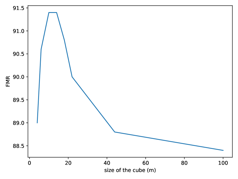
Figure 5: Feature Match Recall (FMR) of MS-SVConv (3) on ETH 8-scenes with respect to the size of the crop of our data generation for UDGE. Model pre-trained on ModelNet. These experiments have been done without periodic sampling

B.6 ETH results details

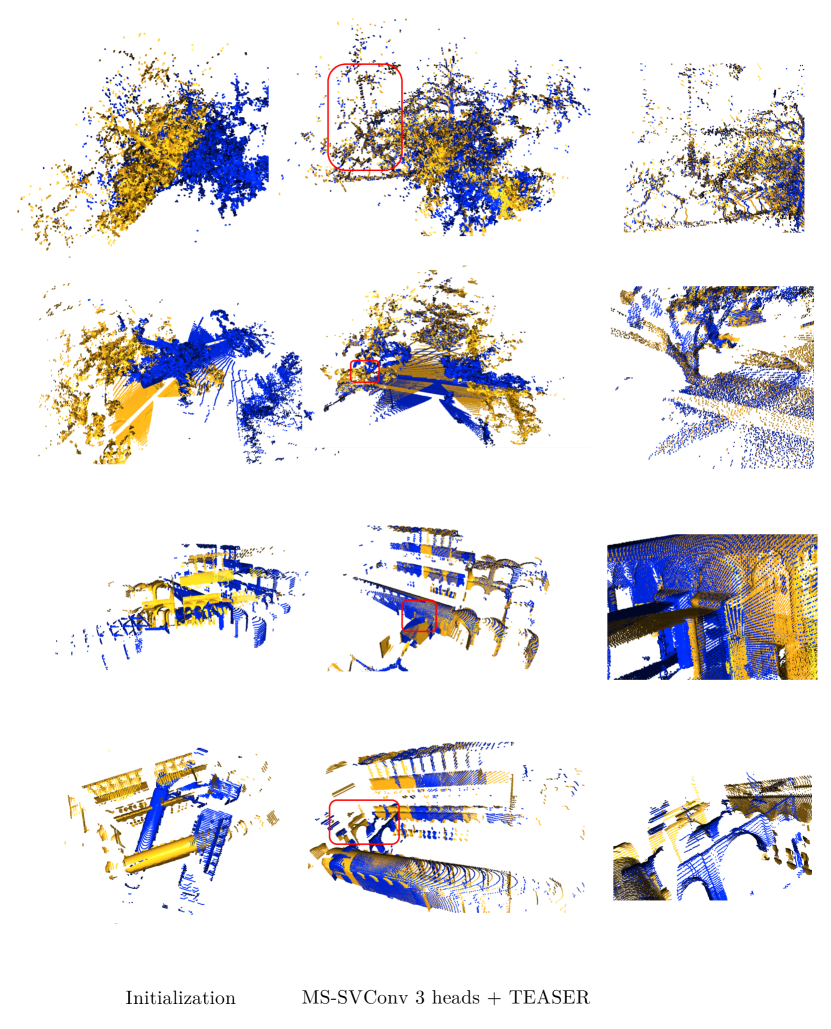
Figure 8: Qualitative results on ETH dataset (model pre-trained on 3DMatch and fine-tuned with UDGE on ETH). The last line shows a failure of MS-SVConv(3).

We present in Table 17 the details of results on the ETH 8-scenes dataset on the different scenes of the dataset. It shows that for the Hauptgebaude scene (scan of a university), results are much lower. Hauptegebaude is more challenging than others because it contains a lot of repetitive patterns (see qualitative results in Figure 8).

Methods	Apart.	Gaz. Sum.	Gaz. Wint.	Haupt.	Plain	Stairs	Wood Aut.	Wood Sum.	Average
Classical methods
FPFH [39]	2/33.1	0/29.2	0/23.6	0/320	0/64.6	4/38.5	0/95.1	0/76.6	0.75/85.1
Patch based deep methods without UDGE
MultiView [28]	83/14.8	42/9.4	52/8.3	47/262	17/21.4	65/15.2	13/12.1	22/9.8	42.6/44.0
DIP [33]	98/8.2	91/6.4	100/5.7	73/5.7	96/9.3	97/6.7	97/6.4	99/6.4	93.9/6.9
U-Net based deep methods without UDGE
D3Feat [4]	96/9.4	78/8.7	93/7.4	54/646	18/54.1	72/12.0	54/10.5	51/12.4	64.5/95.0
MS-SVConv(1)	96/8.8	65/8.6	79/7.4	31/554	14/579	63/26.5	51/10.1	52/10.5	56.4/151.0
MS-SVConv(3)	99/8.1	85/7.7	98/5.6	43/533	36/76.1	84/10.5	81/8.7	88/8.0	76.8/82.2
U-Net based deep methods with UDGE
MS-SVConv(1)	100/9.2	89/6.6	100/4.8	53/301	73/10.9	93/7.3	94/6.4	98/5.9	87.5/44.0
MS-SVConv(3)	99/8.8	97/5.9	100/4.5	70/5.5	85/9.8	98/8.5	100/6.1	100/5.7	93.6/6.9

Table 17: Feature Match Recall (FMR) with $\tau_{2}=0.05$ and median Scaled Registration Error (SRE) x1000 per scene on ETH 8-scenes dataset, benchmark of Fontana et al. [16]. All deep methods are pre-trained on 3DMatch. For every method, we compute the transformation using TEASER algorithm [49]. For FMR, higher is better and for SRE, lower is better.

Appendix C Implementation and Protocol

C.1 Implementation details

To manage the experiments, we used the Pytorch Points 3D framework [7]. This framework massively uses the hydra library to manage the hyperparameters, the architectures of the networks, and the data augmentations. For the sparse convolution and sparse tensors, we use the implementation of Pytorch Points 3D that utilizes the torchsparse backend (implementated by Tang et al. [44]). The implementation of Pytorch Points 3D also supports the MinkowskiEngine backend [10], but sparse convolution in torchsparse is faster than in MinkowskiEngine. For all trainings, we use Stochastic Gradient Descent with momentum of 0.8 as optimizer and a batch size of 4. For pre-training, the number of epochs is 400 for ModelNet (around 48h), and 300 for the 3DMatch dataset (around 3 weeks), and the learning rate is $0.1$. For unsupervised transfer learning, the number of epochs is 200 for all datasets (around 2h for TUM, 18h for ETH, and 24h for 3DMatch), and the learning rate is $0.001$.

On 3DMatch, ModelNet, and TUM, the size of the initial voxel is 2 cm and is doubled at every scale. For the ETH dataset (only when we use UDGE), the size of the initial voxel is 4 cm and also doubled at every scale (ETH dataset is sparser than 3DMatch). The choice of the voxel size depends on the point density. The dimension of output descriptors is 32 for every dataset (as most previous published papers).

For the data generation of UDGE, the crop has a cubic shape, the center is a random point, and the size is 2 m for ModelNet, 3 m for 3DMatch and TUM and 10 m for ETH. As for the crop parameter, the periodic sampling parameters will change according to the dataset: for ETH, we uniformly sample $\alpha$ between 15% and 30% and the period $T$ between 4 cm and 16 cm. For the TUM dataset, we uniformly sample $\alpha$ between 10% and 40% and the period $T$ between 2 cm and 8 cm. For 3DMatch, we do not use periodic sampling as point clouds are uniform.

Finally, we perform classical data augmentation (same for all datasets) such as random rotation around all axes, random scale between 0.9 and 1.2 and random Gaussian noise with $\sigma$ equals to 0.7 cm for TUM and 3DMatch and 1 cm for ETH and ModelNet.

To compute the transformation, we always use the TEASER algorithm [49] (with the main parameter noise bound fixed at $\tau_{1}=0.1$). We choose TEASER over RANSAC because, TEASER is faster. For every experiment, we sample randomly 5000 random points to evaluate point cloud matching. The experiments were done on a computer with a GPU GTX 1080Ti and a CPU Intel(R) Core(TM) i7-4790K.

C.2 Architecture of the network

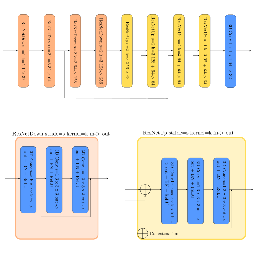
Figure 6: Architecture of one head of our U-Net network (BN means Batch Normalization).

In Figure 6, we report the detailed architecture of a U-Net of MS-SVConv. Because the weights are shared when using MS-SVConv with $S$ heads, the model still has around 9 million parameters in total. The only difference is in the additional MLP shared between all points with FC(S*d,d), which gives 3104 additional parameters for MS-SVConv(3), i.e. three heads with a descriptor of size 32. The architecture of MS-SVConv(1) and FCGF [11] are almost similar but MS-SVConv has one supplementary ResBlock. MS-SVConv is also faster than FCGF: FCGF uses the library MinkowskiEngine while MS-SVConv uses the torchsparse library. For the evaluation, contrary to [4, 33, 19, 2], FCGF [11] does not perform a symmetric test when computing the FMR. This is why, results of FCGF are lower in term of FMR.

C.3 Protocol and metrics on ETH dataset

Methods	Gaz. Sum.	Gaz. Wint	Wood Aut.	Wood Sum.	Average
Classical methods
FPFH [39]	38.6	14.2	14.8	20.8	22.1
SHOT [40]	73.9	45.7	60.9	64.0	61.1
Patch based deep methods without UDGE
3DSmoothNet [19]	62.8	76.9	66.3	78.8	72.1
MultiView [28]	89.5	85.9	81.3	95.1	92.3
DIP [33]	90.8	88.6	96.5	95.2	92.8
SpinNet [2]	92.9	91.7	92.2	94.4	92.8
GeDI [32]	98.9	96.5	97.4	100	98.2
U-Net deep methods without UDGE
FCGF [11]	22.8	10.0	14.8	16.8	16.1
D3Feat [4]	85.9	63.0	49.6	48.0	61.6
MS-SVConv(1)	58.2	23.2	27.0	31.2	34.9
MS-SVConv(3)	89.3	68.1	63.5	65.6	71.8
U-Net deep methods with UDGE
MS-SVConv(1)	86.4	90.0	85.2	90.4	88.0
MS-SVConv(3)	95.7	100	100	100	98.9

Table 18: Feature Match Recall (FMR) on ETH 4-scenes with the benchmark of Gojcic et al. [19] with $\tau_{1}=10$ cm and $\tau_{2}=0.05$. Results from other methods are from published papers. All networks are pre-trained on indoor 3DMatch.

For our tests on the ETH dataset, we followed Fontana et al.’s protocol [16] and Gojcic et al.’s protocol [19]. Fontana et al.’s protocol is more rigorous and uses eight scenes instead of four. Fontana et al. also introduce the Scaled Registration Error (SRE) to evaluate the transformation found by registration methods. Usually, we use a metric based on the rotation error or the translation error. Even if these metrics are useful, they suffer from several problems: there are two measures instead of one, so in some cases, comparison is not possible. Moreover, these metrics depends on whether the point cloud is centered or not. For example, if the point cloud is at 100 m from the center of rotation, a small rotation error of 2 degrees will bring a translation error of around 3 m. To get the results of previous published methods on ETH 8-scenes (Fontana et al.’s protocol [16]), we had to compute them by ourselves using online code. The following section will present the details of the choices made using the available codes of published methods.

C.4 Experiment details for tested method on ETH-8 scenes

We present the experimental details for the methods tested on ETH 8-scenes following the Fontana et al.’s protocol [16]. We have varied the different parameters of all these methods to keep only the best results on ETH.

C.4.1 FPFH [39]

We use the implementation of Open3D [57]. We down-sample the point cloud with a voxel size of 6 cm and we choose 5000 random points. To compute descriptors, we use a radius of 50 cm and use the 30 nearest neighbors to compute normals.

C.4.2 DIP [33]

For DIP, we first down-sample the point cloud with a voxel size of 6 cm. We use DIP on 5000 random points. The patch is a ball with a radius of $60\sqrt{3}=104$ cm. We use $p_{\rho}=0$. The model was provided by the authors (trained on 3DMatch).

C.4.3 D3Feat [4]

For D3Feat, we down-sample the point cloud with a voxel size of 6 cm (as in the implementation). We use the Tensorflow implementation. We double the scale of the kernel points to increase the receptive field as done by Bai et al. [4]. We use the model trained using the contrastive loss provided by the authors (we noticed that the model trained with the circle loss has worse results). We choose the 5000 points with the best score to compute the Feature Match Recall and the Scaled Registration Error.

C.4.4 MultiView [28]

For MultiView, we used the pre-trained model provided by the authors. We down-sample the point cloud with a voxel size of 6 cm and took 5000 random points.

Appendix D Qualitative results on the 3DMatch, ETH and TUM dataset

We show in Figures 7, 8 and 9 images of point cloud registration using MS-SVConv(3) for the 3DMatch, ETH, and TUM dataset.

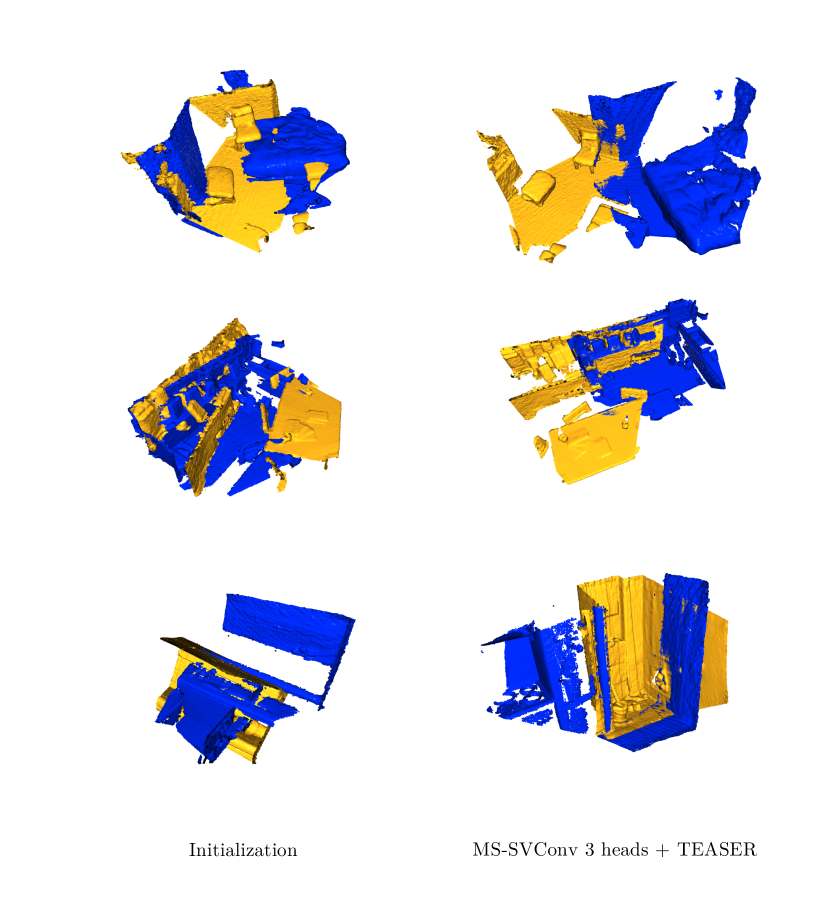
Figure 7: Qualitative results on 3DMatch (supervised learning). We can see that even with few structure and low overlap, MS-SVConv(3) can find the transformation between the pair of scenes.

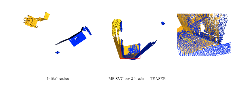
Figure 9: Qualitative results on TUM dataset (model pre-trained on 3DMatch and fine-tuned with UDGE on TUM).

References

- [1] Dror Aiger, Niloy J. Mitra, and Daniel Cohen-Or. 4-points congruent sets for robust pairwise surface registration. ACM Trans. Graph., 27(3):1–10, Aug. 2008.
- [2] Sheng Ao, Qingyong Hu, Bo Yang, Andrew Markham, and Yulan Guo. SpinNet: Learning a General Surface Descriptor for 3D Point Cloud Registration. arXiv e-prints, page arXiv:2011.12149, Nov. 2020.
- [3] Yasuhiro Aoki, Hunter Goforth, Rangaprasad Arun Srivatsan, and Simon Lucey. Pointnetlk: Robust and efficient point cloud registration using pointnet. In 2019 IEEE/CVF Conference on Computer Vision and Pattern Recognition (CVPR), pages 7156–7165, 2019.
- [4] Xuyang Bai, Zixin Luo, Lei Zhou, Hongbo Fu, Long Quan, and Chiew-Lan Tai. D3feat: Joint learning of dense detection and description of 3d local features. In 2020 IEEE/CVF Conference on Computer Vision and Pattern Recognition (CVPR), pages 6358–6366, 2020.
- [5] Paul J. Besl and Neil D. McKay. A method for registration of 3-d shapes. IEEE Transactions on Pattern Analysis and Machine Intelligence, 14(2):239–256, 1992.
- [6] Sofien Bouaziz, Andrea Tagliasacchi, and Mark Pauly. Sparse iterative closest point. Computer Graphics Forum, 32(5):113–123, 2013.
- [7] Thomas Chaton, Nicolas Chaulet, Sofiane Horache, and Loic Landrieu. Torch-points3d: A modular multi-task framework for reproducible deep learning on 3d point clouds. In 2020 International Conference on 3D Vision (3DV), pages 1–10, 2020.
- [8] Sungjoon Choi, Qian-Yu Zhou, and Vladlen Koltun. Robust reconstruction of indoor scenes. In 2015 IEEE Conference on Computer Vision and Pattern Recognition (CVPR), pages 5556–5565, 2015.
- [9] Christopher Choy, Wei Dong, and Vladlen Koltun. Deep global registration. In 2020 IEEE/CVF Conference on Computer Vision and Pattern Recognition (CVPR), pages 2511–2520, 2020.
- [10] Christopher Choy, JunYoung Gwak, and Silvio Savarese. 4d spatio-temporal convnets: Minkowski convolutional neural networks. In 2019 IEEE/CVF Conference on Computer Vision and Pattern Recognition (CVPR), pages 3070–3079, 2019.
- [11] Christopher Choy, Jaesik Park, and Vladlen Koltun. Fully convolutional geometric features. In Proceedings of the IEEE/CVF International Conference on Computer Vision (ICCV), October 2019.
- [12] Angela Dai, Matthias Nießner, Michael Zollöfer, Shahram Izadi, and Christian Theobalt. Bundlefusion: Real-time globally consistent 3d reconstruction using on-the-fly surface re-integration. ACM Transactions on Graphics 2017 (TOG), 2017.
- [13] Haowen Deng, Tolga Birdal, and Slobodan Ilic. Ppf-foldnet: Unsupervised learning of rotation invariant 3d local descriptors. In Vittorio Ferrari, Martial Hebert, Cristian Sminchisescu, and Yair Weiss, editors, Computer Vision – ECCV 2018, pages 620–638, Cham, 2018. Springer International Publishing.
- [14] Haowen Deng, Tolga Birdal, and Slobodan Ilic. Ppfnet: Global context aware local features for robust 3d point matching. In 2018 IEEE/CVF Conference on Computer Vision and Pattern Recognition, pages 195–205, 2018.
- [15] Martin A. Fischler and Robert C. Bolles. Random sample consensus: A paradigm for model fitting with applications to image analysis and automated cartography. Commun. ACM, 24(6):381–395, June 1981.
- [16] Simone Fontana, Daniele Cattaneo, Augusto L. Ballardini, Matteo Vaghi, and Domenico G. Sorrenti. A benchmark for point clouds registration algorithms. Robotics and Autonomous Systems, 140:103734, 2021.
- [17] Natasha Gelfand, Leslie Ikemoto, Szymon Rusinkiewicz, and Marc Levoy. Geometrically stable sampling for the icp algorithm. In Fourth International Conference on 3-D Digital Imaging and Modeling (3DIM), pages 260–267, 2003.
- [18] Zan Gojcic, Caifa Zhou, Jan D. Wegner, Leonidas J. Guibas, and Tolga Birdal. Learning multiview 3d point cloud registration. In 2020 IEEE/CVF Conference on Computer Vision and Pattern Recognition (CVPR), pages 1756–1766, 2020.
- [19] Zan Gojcic, Caifa Zhou, Jan D. Wegner, and Andreas Wieser. The perfect match: 3d point cloud matching with smoothed densities. In 2019 IEEE/CVF Conference on Computer Vision and Pattern Recognition (CVPR), pages 5540–5549, 2019.
- [20] Y. Guo, H. Wang, Q. Hu, H. Liu, L. Liu, and M. Bennamoun. Deep learning for 3d point clouds: A survey. IEEE Transactions on Pattern Analysis and Machine Intelligence, pages 1–1, 2020.
- [21] Maciej Halber and Thomas Funkhouser. Fine-to-coarse global registration of rgb-d scans. In 2017 IEEE Conference on Computer Vision and Pattern Recognition (CVPR), pages 6660–6669, 2017.
- [22] Xian-Feng Han, Jesse Sheng Jin, Juan Xie, Ming-Jie Wang, and Wei Jiang. A comprehensive review of 3d point cloud descriptors. arXiv:1802.02297 [cs], Feb. 2018.
- [23] Qingyong Hu, Bo Yang, Linhai Xie, Stefano Rosa, Yulan Guo, Zhihua Wang, Niki Trigoni, and Andrew Markham. Randla-net: Efficient semantic segmentation of large-scale point clouds. In 2020 IEEE/CVF Conference on Computer Vision and Pattern Recognition (CVPR), pages 11105–11114, 2020.
- [24] Shengyu Huang, Zan Gojcic, Mikhail Usvyatsov, Andreas Wieser, and Konrad Schindler. Predator: Registration of 3d point clouds with low overlap. In Proceedings of the IEEE/CVF Conference on Computer Vision and Pattern Recognition (CVPR), pages 4267–4276, June 2021.
- [25] Xiaoshui Huang, Guofeng Mei, and Jian Zhang. Feature-metric registration: A fast semi-supervised approach for robust point cloud registration without correspondences. In 2020 IEEE/CVF Conference on Computer Vision and Pattern Recognition (CVPR), pages 11363–11371, 2020.
- [26] Andrew E. Johnson and Martial Hebert. Using spin images for efficient object recognition in cluttered 3d scenes. IEEE Transactions on Pattern Analysis and Machine Intelligence, 21(5):433–449, 1999.
- [27] Sehyung Lee, Makiko Negishi, Hidetoshi Urakubo, Haruo Kasai, and Shin Ishii. Mu-net: Multi-scale u-net for two-photon microscopy image denoising and restoration. Neural Networks, 125:92–103, 2020.
- [28] Lei Li, Siyu Zhu, Hongbo Fu, Ping Tan, and Chiew-Lan Tai. End-to-end learning local multi-view descriptors for 3d point clouds. In 2020 IEEE/CVF Conference on Computer Vision and Pattern Recognition (CVPR), pages 1916–1925, 2020.
- [29] Xueqian Li, Jhony Kaesemodel Pontes, and Simon Lucey. Pointnetlk revisited. In Proceedings of the IEEE/CVF Conference on Computer Vision and Pattern Recognition (CVPR), pages 12763–12772, June 2021.
- [30] Weixin Lu, Guowei Wan, Yao Zhou, Xiangyu Fu, Pengfei Yuan, and Shiyu Song. Deepvcp: An end-to-end deep neural network for point cloud registration. In 2019 IEEE/CVF International Conference on Computer Vision (ICCV), pages 12–21, 2019.
- [31] Daniel Maturana and Sebastian Scherer. Voxnet: A 3d convolutional neural network for real-time object recognition. In 2015 IEEE/RSJ International Conference on Intelligent Robots and Systems (IROS), pages 922–928, 2015.
- [32] Fabio Poiesi and Davide Boscaini. Generalisable and distinctive 3D local deep descriptors for point cloud registration. arXiv e-prints, page arXiv:2105.10382, May 2021.
- [33] Fabio Poiesi and Davide Poiesi. Distinctive 3d local deep descriptors. In IEEE Proc. of Int’l Conference on Pattern Recognition (ICPR), Milan, IT, 2021.
- [34] François Pomerleau, Ming Liu, Francis Colas, and Roland Siegwart. Challenging data sets for point cloud registration algorithms. The International Journal of Robotics Research, 31(14):1705–1711, Dec. 2012.
- [35] Charles R. Qi, Hao Su, Kaichun Mo, and Leonidas J. Guibas. Pointnet: Deep learning on point sets for 3d classification and segmentation. In 2017 IEEE Conference on Computer Vision and Pattern Recognition (CVPR), pages 77–85, 2017.
- [36] Charles R. Qi, Li Yi, Hao Su, and Leonidas J. Guibas. Pointnet++: Deep hierarchical feature learning on point sets in a metric space. In Proceedings of the 31st International Conference on Neural Information Processing Systems, NIPS’17, page 5105–5114, Red Hook, NY, USA, 2017.
- [37] Xavier Roynard, Jean-Emmanuel Deschaud, and François Goulette. Classification of Point Cloud Scenes with Multiscale Voxel Deep Network. arXiv e-prints, page arXiv:1804.03583, Apr. 2018.
- [38] Szymon Rusinkiewicz and Marc Levoy. Efficient variants of the icp algorithm. In Proceedings Third International Conference on 3-D Digital Imaging and Modeling, pages 145–152, 2001.
- [39] Radu Bogdan Rusu, Nico Blodow, and Michael Beetz. Fast point feature histograms (fpfh) for 3d registration. In 2009 IEEE International Conference on Robotics and Automation, pages 3212–3217, 2009.
- [40] Samuele Salti, Federico Tombari, and Luigi Di Stefano. Shot: Unique signatures of histograms for surface and texture description. Computer Vision and Image Understanding, 125:251–264, 2014.
- [41] Jamie Shotton, Ben Glocker, Christopher Zach, Shahram Izadi, Antonio Criminisi, and Andrew Fitzgibbon. Scene coordinate regression forests for camera relocalization in rgb-d images. In Proc. Computer Vision and Pattern Recognition (CVPR). IEEE, June 2013.
- [42] Jürgen Sturm, Nikolas Engelhard, Felix Endres, Wolfram Burgard, and Daniel Cremers. A benchmark for the evaluation of rgb-d slam systems. In 2012 IEEE/RSJ International Conference on Intelligent Robots and Systems, pages 573–580, 2012.
- [43] Hang Su, Subhransu Maji, Evangelos Kalogerakis, and Erik Learned-Miller. Multi-view convolutional neural networks for 3d shape recognition. In 2015 IEEE International Conference on Computer Vision (ICCV), pages 945–953, 2015.
- [44] Haotian Tang, Zhijian Liu, Shengyu Zhao, Yujun Lin, Jin Lin, Hanrui Wang, and Song Han. Searching efficient 3d architectures with sparse point-voxel convolution. In European Conference on Computer Vision (ECCV), 2020.
- [45] Hugues Thomas, Charles R. Qi, Jean-Emmanuel Deschaud, Beatriz Marcotegui, François Goulette, and Leonidas J. Guibas. Kpconv: Flexible and deformable convolution for point clouds. In 2019 IEEE/CVF International Conference on Computer Vision (ICCV), pages 6410–6419, 2019.
- [46] Yue Wang and Justin M. Solomon. Deep closest point: Learning representations for point cloud registration. In 2019 IEEE/CVF International Conference on Computer Vision (ICCV), pages 3522–3531, 2019.
- [47] Yue Wang and Justin M. Solomon. Prnet: Self-supervised learning for partial-to-partial registration. In 33rd Conference on Neural Information Processing Systems, 2019.
- [48] Zhirong Wu, Shuran Song, Aditya Khosla, Fisher Yu, Linguang Zhang, Xiaoou Tang, and Jianxiong Xiao. 3d shapenets: A deep representation for volumetric shapes. In 2015 IEEE Conference on Computer Vision and Pattern Recognition (CVPR), pages 1912–1920, 2015.
- [49] Heng Yang, Jingnan Shi, and Luca Carlone. Teaser: Fast and certifiable point cloud registration. IEEE Transactions on Robotics, pages 1–20, 2020.
- [50] Jiaolong Yang, Hongdong Li, Dylan Campbell, and Yunde Jia. Go-icp: A globally optimal solution to 3d icp point-set registration. IEEE Transactions on Pattern Analysis and Machine Intelligence, 38(11):2241–2254, 2016.
- [51] Zi Jian Yew and Gim Hee Lee. Rpm-net: Robust point matching using learned features. In 2020 IEEE/CVF Conference on Computer Vision and Pattern Recognition (CVPR), pages 11821–11830, 2020.
- [52] Yijun Yuan, Jiawei Hou, Andreas Nüchter, and Sören Schwertfeger. Self-supervised point set local descriptors for point cloud registration. Sensors, 21(2), 2021.
- [53] Andy Zeng, Shuran Song, Matthias Nießner, Matthew Fisher, Jiangxiong Xiao, and Thomas Funkhouser. 3dmatch: Learning local geometric descriptors from rgb-d reconstructions. In 2017 IEEE Conference on Computer Vision and Pattern Recognition (CVPR), pages 199–208, 2017.
- [54] Zaiwei Zhang, Rohit Girdhar, Armand Joulin, and Ishan Misra. Self-Supervised Pretraining of 3D Features on any Point-Cloud. arXiv e-prints, page arXiv:2101.02691, Jan. 2021.
- [55] Yongheng Zhao, Tolga Birdal, Haowen Deng, and Federico Tombari. 3d point capsule networks. In 2019 IEEE/CVF Conference on Computer Vision and Pattern Recognition (CVPR), pages 1009–1018, 2019.
- [56] Qian-Yi Zhou, Jaesik Park, and Vladlen Koltun. Fast global registration. In Bastian Leibe, Jiri Matas, Nicu Sebe, and Max Welling, editors, Computer Vision – ECCV 2016, pages 766–782, Cham, 2016. Springer International Publishing.
- [57] Qian-Yi Zhou, Jaesik Park, and Vladlen Koltun. Open3D: A Modern Library for 3D Data Processing. arXiv e-prints, page arXiv:1801.09847, Jan. 2018.