Testing identity of collections of quantum states: sample complexity analysis

Abstract

We study the problem of testing identity of a collection of unknown quantum states given sample access to this collection, each state appearing with some known probability. We show that for a collection of $d$-dimensional quantum states of cardinality $N$, the sample complexity is $O(\sqrt{N}d/\epsilon^{2})$, with a matching lower bound, up to a multiplicative constant. The test is obtained by estimating the mean squared Hilbert-Schmidt distance between the states, thanks to a suitable generalization of the estimator of the Hilbert-Schmidt distance between two unknown states by Bădescu, O’Donnell, and Wright (https://dl.acm.org/doi/10.1145/3313276.3316344).

1 Introduction

The closeness between quantum states can be quantified according to a variety of unitarily invariant distance measures, with different operational interpretations [Hay17b]. Given access to copies of some unknown states, a fundamental inference problem is to tell if the states are equal or distant more than $\epsilon$, according to some unitarily invariant distance. Since this problem does not require to completely reconstruct the unknown states with tomography protocols, optimal algorithms require less copies than full tomography to answer successfully [BOW19]. Due to unitarily invariance, efficient algorithms can also be guessed by symmetry arguments [Hay17].

In this work we study the problem of testing identity of a collection of unknown quantum states given sample access to the collection. We show that for a collection of $d$-dimensional quantum states of cardinality $N$, the sample complexity is $O(\sqrt{N}d/\epsilon^{2})$, which is optimal up to a constant. We assume a sampling model access, where each state appears with some known probability, adapting [LRR13, DK16] to the quantum case. We also consider a Poissonized version of the sampling model, where the number of each copies of a state is a Poissonian random variable, and we show that the sample complexity of the two models is the same. This problem is an example of property testing, a concept developed in computer science [Gol17], and applied to hypothesis testing of distributions [Can20] and quantum states and channels [MW16]. At variance with optimal asymptotic error rates studied in statistical classical and quantum hypothesis testing [LR06, Hay17b], the sample complexity captures finite size effect in inference problems, as it expresses the number of samples required to successfully execute an inference task in terms of the extensive parameters of the problem, in our case the dimension $d$ and the cardinality $N$ of the collection. The interest in these kind of questions in the classical case has been motivated by the importance of the study of big data sources; a similar motivation holds for the quantum case, since outputs of fully functional quantum computers will also live in high-dimensional spaces.

1.1 Results

Given a collection of $d$-dimensional quantum states $\{\rho_{i}\}_{i=1,...,N}$, and a probability distribution $p_{i}$ ($0<p_{i}<1$), we consider a sampling model [LRR13, DK16] where we have access to $M$ copies of the density matrix

$$\rho=\sum_{i=1}^{N}p_{i}\outerproduct{i}{i}\otimes\rho_{i},$$ (1)

where $\{\ket{i}\}_{i=1,...,N}$ is an orthonormal basis of a $N$ dimensional (classical) register. We are promised that one of the two following properties holds:

• Case $\mathsf{A}$: $\rho_{1}=\rho_{2}=...=\rho_{N}$, which can be equivalently stated by saying that there exists a $d$-dimensional state $\sigma$ such that $\sum_{i}p_{i}D_{\mathrm{Tr}}(\rho_{i},\sigma)=0$, with $D_{\mathrm{Tr}}$ the trace distance [Hay17b];

• Case $\mathsf{B}$: For any $d$-dimensional state $\sigma$ it holds $\sum_{i}p_{i}D_{\mathrm{Tr}}(\rho_{i},\sigma)>\epsilon$.

Our goal is to find the values of $M$ for which there is a two-outcome test that can discriminate the two cases with high probability of success. Explicitly, indicating with "accept" and "reject" the outcomes of the test, we require the probability of getting "accept" to be larger than $2/3$ in case $\mathsf{A}$, and smaller than $1/3$ in case $\mathsf{B}$, i.e.

$$\left\{\begin{array}[]{l}P(\mbox{{test $\mapsto$ "accept"} }|\mbox{Case $\mathsf{A}$})>2/3\;,\\ \\ P(\mbox{{test $\mapsto$ "accept"} }|\mbox{Case $\mathsf{B}$})<1/3\;.\end{array}\right.$$ (5)

Note that the values $2/3$ and $1/3$ are by convention and, as long as we are interested in the sample complexity only up to a scaling factor, can be replaced by any pair of constants $c,s$, respectively, such that $1>c>s>0$. The main result of the paper is to provide an estimate of necessary and sufficient values of $M$ to fulfill the above conditions. We use the notations $O(f(d,N,\epsilon))$ and $\Omega(g(d,N,\epsilon))$ to indicate respectively upper and lower bounds to sample complexities, up to multiplicative constants. If lower and upper bounds which differ by a multiplicative constant can be obtained, the sample complexity is considered to be determined and indicated as $\Theta(f(d,N,\epsilon))=\Theta(g(d,N,\epsilon))$.

Specifically we prove the following results:

Theorem 1.1.

For any $\epsilon>0$, given access to $O\left(\frac{\sqrt{N}d}{\epsilon^{2}}\right)$ samples of the density matrix $\rho$ of Eq. (1), there is an algorithm which can distinguish with high probability whether

• $\sum_{i}p_{i}D_{\mathrm{Tr}}(\rho_{i},\sigma)>\epsilon$ for every state $\sigma$ (Case $\mathsf{B}$), or

• there exists a state $\sigma$ such that $\sum_{i}p_{i}D_{\mathrm{Tr}}(\rho_{i},\sigma)=0$ (that is, all the states $\rho_{i}$ are equal, Case $\mathsf{A}$).

Theorem 1.2.

For any $\epsilon>0$, any algorithm which can distinguish with high probability whether

• $\sum_{i}p_{i}D_{\mathrm{Tr}}(\rho_{i},\sigma)>\epsilon$ for every state $\sigma$ (Case $\mathsf{B}$), or

• there exists a state $\sigma$ such that $\sum_{i}p_{i}D_{\mathrm{Tr}}(\rho_{i},\sigma)=0$ (that is, all the states $\rho_{i}$ are equal, Case $\mathsf{A}$),

given access to $M$ copies of the density matrix $\rho$ of Eq. (1), requires at least $M=\Omega\left(\frac{\sqrt{N}d}{\epsilon^{2}}\right)$ copies.

The proof of Theorem 1.2 is presented in Sec. 4 and it relies on the fact that a test working with $M$ copies could be used to discriminate between two states which are close in trace distance unless $M=\Omega\left(\frac{\sqrt{N}d}{\epsilon^{2}}\right)$. These states are obtained as average inputs $\rho_{A}$ and $\rho_{B}$ of the form of Eq. (1) for two different set of collections of states: in the first case the set is made of only one collection consisting of maximally mixed states (thus satisfying case $\mathsf{A}$), and in the second the set of collections is such that its elements satisfy case $\mathsf{B}$ with high probability. The technical contributions of this proof are (a) a lower bound on the probability that a collection of random states with spectrum $s_{\epsilon}=(\frac{1+\epsilon}{d},\frac{1-\epsilon}{d},...,\frac{1+\epsilon}{d},\frac{1-\epsilon}{d})$ has large average trace distance to their average state; (b) an upper bound on the distance between $\rho_{A}$ and $\rho_{B}$ being the average input state over collections of random states with spectrum $s_{\epsilon}$. Both results could be useful elsewhere.

The derivation of the upper bound for $M$ given in Theorem 1.1 is instead presented in Sec. 3 and it is obtained by constructing an observable $\mathcal{D}_{M}$ whose expected value is the mean squared Hilbert-Schmidt distance between the states $\rho_{i}$, and we bound the variance of the estimator. By relating the mean squared Hilbert-Schmidt distance to $\sum_{i}p_{i}D_{\mathrm{Tr}}(\rho_{i},\sum_{i}p_{i}\rho_{i})$ we obtain the test of the theorem. This strategy follow closely the methods of [BOW19] (for $N=2$), although with some relevant changes due to the fact that we are not requiring a fixed number of copies of each state $\rho_{i}$, like in [BOW19]. This difference is relevant from a conceptual point of view, since having an arbitrary number of copies of each state is a stronger type of access with respect to the sampling model, and closer to the query model (we discussed the different applicability scenario in the following section). It is also relevant from a technical point of view, since it is not immediate to devise an estimator for which the analysis can be completed. In fact, the analysis exploits a Poissonization trick [LRR13] where the number of copies $M$ is not fixed but a random variable, extracted from a Poisson distribution with average $\mu$, $\text{Poi}_{\mu}(M):=\frac{e^{-\mu}\mu^{M}}{M!}$ (summarized later on by the notation $M\sim\text{Poi}_{\mu}$). We then look for a test which can be performed by a two-outcome POVM $\{E_{0}^{(M)},E_{1}^{(M)}\}$ for each $M$. Poissonization is a standard technique that allows the for some useful simplification of the analysis by getting rid of unwanted correlations (more on this in Sec. 3.1). The equivalence of the Poissonized model with the original one is formalised in Appendix A.

Analogously to [BOW19] we can refine the upper bound when the states in the collection have low rank. Given the state $\rho$ of Eq. (1), we define its reduced average density matrix

$$\bar{\rho}:=\sum_{i=1}^{N}p_{i}\rho_{i}\;,$$ (6)

In particular, when $\bar{\rho}$ is $\eta$-close to rank $k$, that is, the sum of its $k$ largest eigenvalues is larger than $1-\eta$, we can refine Theorem 1.1:

Theorem 1.3.

If the density matrix $\bar{\rho}$ of Eq. (6) is $\eta$-close to rank $k$, given access to $O\left(\frac{\sqrt{N}k}{\epsilon^{2}}\right)$ samples of $\rho$ there exists an algorithm which can distinguish with high probability whether $\sum_{i}p_{i}D_{\mathrm{Tr}}(\rho_{i},\sigma)>\epsilon+\eta$ for every state $\sigma$, or there exists a state $\sigma$ such that $\sum_{i}p_{i}D_{HS}(\rho_{i},\sigma)<8(2-\sqrt{2})\epsilon$.

1.2 Motivation of the setting

In this section we present a couple of physical settings which give rise to the sampling models discussed in Sec.1.1, as both the original model and the Poissonized model refer to natural scenarios for a certification task.

Independent sources setting (panel (a) of Figure 1). It is fair to assume that each copy of the states is produced by a device $\mathcal{S}_{i}$ that require some physical time to run, and produces the expected state with some probability. Moreover, assume that the number of produced copies of $\rho_{i}$ by $\mathcal{S}_{i}$ at any time $T$ is given by a Poisson distribution with rate $r_{i}$ and average $r_{i}T$, i.e. $P_{T}(m_{i})=\text{Poi}_{r_{i}T}(m_{i})=\frac{(r_{i}T)^{m_{i}}e^{r_{i}T}}{m_{i}!}$. With this assumption, it also holds that the probability that a total of $M=m_{1}+...+m_{N}$ copies is produced in the time $T$ is $P_{T}(M)=\frac{(T\sum_{i=1}^{N}r_{i})^{M}e^{T\sum_{i=1}^{N}r_{i}}}{M!}$. The Poissonized sampling model (where the probabilities of getting $m_{i}$ copies of $\rho_{i}$ are given by a Poisson distribution with average $p_{i}\mu$, see Eq. (41)) is an adequate representation of the setting where we want to do our certification test with all the copies that are produced in a certain timeframe $T$, see panel (a) of Figure 1.

On the other hand, if we decide to run the test as soon the total number of copies corresponds to the desired number $M$, we end up in the original sample model. Indeed, if $T_{M}$ is the random variable equal to the time at which the total number of copies is $M$, we have that the probability of finding a vector $\vec{m}=(m_{1},...,m_{N})$ of number of copies $\rho_{1},...,\rho_{N}$, respectively, conditioned on $m_{1}+...+m_{N}=M$ at the time $T_{M}$, is

$$P(\vec{m}|M)=\int_{0}^{\infty}p(T_{M}=T)P_{T}(\vec{m}|M)dT,\\$$ (7)

where $p(T_{M}=T)$ is the probability density for the stopping time $T_{M}$, and

$$P_{T}(\vec{m}|M) =P_{T}(\vec{m},M)/P_{T}(M)=P_{T}(\vec{m})/P_{T}(M)=\prod_{j=1}^{N}P_{T}(m_{j})/P_{T}(M)$$ (8)

$$=\frac{M!}{m_{1}!...m_{N}!}\prod_{j=1}^{N}r_{i}^{m_{i}}.$$ (9)

where the first equality comes from the definition of conditional probability, the second comes from the fact that $M$ is completely determined by $\vec{m}$, the third comes from the fact that the components of $\vec{m}$ are independent when conditioning only on $T$, and the last equality comes from writing the probabilities explicitly. Finally, by integrating a constant function, we have

$$P(\vec{m}|M)=\frac{M!}{m_{1}!...m_{N}!}\prod_{j=1}^{N}r_{i}^{m_{i}},$$ (10)

which is the probability distribution of the copies of each $\rho_{i}$ in the original sampling model with $M$ total copies of $\rho$, provided that $r_{i}=p_{i}$.

These two situations can be compared with the setting of the query model, already considered in [Yu23]; in that case, we are allowed to ask for any number of copies of each state $\rho_{i}$ in the collection, and the sample complexity is measured with respect to the total number of copies requested. This type of access is clearly stronger with respect to the sampling models, and indeed the sample complexity is lower, being $\Theta(d/\epsilon^{2})$. However, assuming there is a finite rate of copies/time, the sampling model captures better the actual physical time required to generate the copies for the test.

On the other hand, the validity of the assumption that the number of copies of each state is generated by a Poisson distribution can be questioned. By the law of rare events, this is a realistic approximation if each source actually corresponds to many independent sources, each of which produces a copy of the state with very small probability, such that the total rate of production of state is finite. In particular, the following bound on the variational distance between the Poisson distribution and sum of independent Bernoulli random variables $X_{i}\sim(p_{i},1-p_{i})$ holds [LC60]: $\sum_{k=0}^{\infty}|P(\sum_{i=1}^{n}X_{i}=k)-\frac{(\sum_{i=1}^{n}p_{i})^{k}e^{-(\sum_{i=1}^{n}p_{i})}}{k!}|<2(\sum_{i=1}^{n}p_{i}^{2})$. The approximation with i.i.d. Bernoulli variables was considered, for example, for entanglement certification of single-photon pairs produced with spontaneus parametric down conversion [HTM08] in the asymptotic setting, with proposed tests implemented experimentally [Hay+06]. In these cases the single-photon pairs are produced with a very small probability from a single beam, but with a finite rate if the number of beams is large, and the distribution of the total number of pairs is approximated by a Poisson distribution. In any case, since any probabilistic model can be simulated or can simulate our sampling model, simply simulating the desired probability distribution on a classical computer and waiting for enough copies, our protocol gives respectively upper or lower bounds on the sample complexity. These bounds are tight if the simulation is efficient, that is it requires the same number of copies, up to a constant multiplicative factor. It would be interesting to characterize which sampling models can efficiently simulate or be simulated by the Poissonized model, but we will not discuss this issue here.

Noisy measurement setting (panel (b) of Figure 1). We point out another setting where the sampling model can represent a realistic situation in the lab: suppose that some preparation procedure $\mathcal{S}$ ends with some measurement, but different outcomes of the measurement are expected to correspond to the same desired state. An example could be the case if our preparation apparatus has interacted with an environment, and we measure the environment. Since the outcome of the measurement at the preparation stage is random, the procedure prepares in principle different states for each measurement outcome. The classical-quantum state we obtain, possibly after post-selection of acceptable measurement outcomes, will have the form in Eq. (1). The goal of the test is to certify if a source of states of this kind is stable or not.

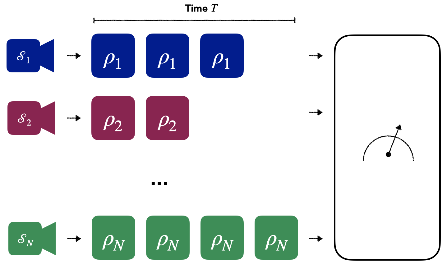
(a)

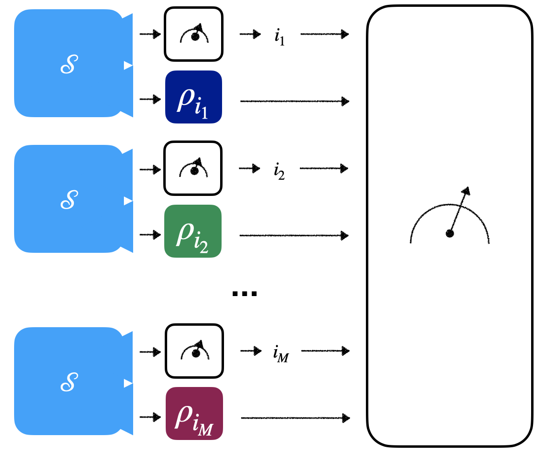
(b)

Figure 1: Two settings to which our model applies. In a) independent sources produce a random number, Poisson distributed, of copies of a state in a time $T$. In b), a measurement procedure prepares labeled states, each label appearing with some probability.

Finally, we point out similarities with the problem of quantum change point detection [AH11, Sen+16, SCMT17, SMVMT18, FHC23], in which a sequence of unknown states is presented, and it is asked if they are all equal or not. An additional question is to identify the points where the states change. With our algorithm, we are able to answer correctly to the change point problem when we know that there could be a change point among $N-1$ possible change points, which have distances between them given by Poissonian random variables. It would be interesting if the analysis and the techniques of the present paper could be extended to address the change point problem more directly.

1.3 Related work

1.3.1 Classical distribution testing

For an overview of learning properties of a classical distribution in the spirit of property testing, we refer to [Gol17, Can20]. We report a partial list of results which are of direct interest for this paper, about testing symmetric properties of distribution in total variation distance. We use the notation $[d]$ for the set $\{1,...,d\}$. Learning a classical distribution over $[d]$ in total variation distance can be done in $O(d/\epsilon^{2})$ samples [Gol17], therefore the interest in testing properties is to get a sample complexity $o(d)$. The problem of testing uniformity was addressed in [GR11] and established to be $O(\sqrt{d}/\epsilon^{2})$ in successive works [Pan08, VV14]. More generally, the sample complexity of identity testing to a known distribution has been established to be $\Theta(\sqrt{d}/\epsilon^{2})$ [VV14, DKN15]. Identity testing for two unknown distribution is $\Theta(\max(d^{1/2}/\epsilon^{2},d^{2/3}/\epsilon^{4/3}))$ [Cha+14]. The problem of testing identity of collection of $N$ distributions was introduced in the classical case in [LRR13] and solved in [DK16], obtaining $\Theta(\max(\sqrt{dN}/\epsilon^{2},d^{2/3}N^{1/3}/\epsilon^{4/3}))$ for the sampling model, where at each sample the tester receives one of $N$ distributions with probabilty $p_{i}$, and $\Theta(\max(\sqrt{d}/\epsilon^{2},d^{2/3}/\epsilon^{4/3}))$ for the query model, where the tester can choose the distribution to call at each sample. A problem related to testing identity of collections is testing independence of a distribution on $\times_{i=1}^{l}[n_{i}]$, which was addressed by [Bat+01, LRR13, AD15] and solved in [DK16], which showed a tight sample complexity $\Theta(\max_{j}(\prod_{i=1}^{l}n_{i}^{1/2}/\epsilon^{1/2},n_{j}^{1/3}\prod_{i=1}^{l}n_{i}^{1/3}/\epsilon^{4/3}))$.

1.3.2 Quantum state testing

It has been shown that the reconstruction of the classical description of an unknown state, quantum tomography, requires $\Theta(d^{2}/\epsilon^{2})$ copies of the state [Haa+17, OW16, OW17]. These algorithms often include, as a subroutine, spectrum learning [ARS88, KW01, HM02, Chr06, Key06], which has sample complexity $O(d^{2}/\epsilon^{2})$ [OW16], although a matching lower bound is available only for the empirical Young diagram estimator [OW15]. These results have been refined in the case the state is known to be close to a state of rank less than $k$. Quantum entropy estimation has been studied in [Ach+20]. The property testing approach to quantum properties has been reviewed in [MW16], where it is also shown that testing identity to a pure state requires $O(1/\epsilon^{2})$. Testing identity to the maximally mixed state takes $\Theta(d/\epsilon^{2})$ [OW15], and the same is true for a generic state and for testing identity between unknown states (with refinements if the state can be approximated by a rank $k$ state) [BOW19]. In [BOW19], identity testing between unknown states is done by first estimating their Hilbert-Schmidt distance with a minimum variance unbiased estimator, developing a general framework for efficient estimators of sums of traces of polynomials of states. This improves on a simple way to estimate the overlap $\Tr[\rho\sigma]$ between two unknown states, the swap test [Buh+01], while optimal estimation of the overlap between pure states with average error figures of merit has been addressed by a series of works [BRS04, BIMT06, LSB06, GI06, Fan+20]. In all of these cases, the algorithms considered are classical post-processing of the measurement used to learn the spectrum of a state, possibly repeated on nested sets of inputs. This measurement can be efficiently implemented, with gate complexity $O(n,\log d,\log 1/\delta)$ [BCH06, Har05, Kro19], where $n$ is the number of copies of the state, and $\delta$ is the precision of the implementation. This measurement is relevant for several quantum information tasks, for example in communication (see e.g. [Hay17, Ben+14]). Testing identity of collections of quantum states in the query model has been established to be $\Theta(d/\epsilon^{2})$ [Yu21], while the sampling model complexity was left open and is addressed in this paper. Independence testing is also addressed in [Yu21], obtaining a sample complexity $O(d_{1}d_{2}/\epsilon^{2})$, which is tight up to logarithmic factors, using the identity test of [BOW19] for testing independence of a state on $\mathbb{C}^{d_{1}}\otimes\mathbb{C}^{d_{2}}$; similar results hold for the multipartite case (see also [HT16] for the asymptotic setting and [Bai+22] for an application of independence testing to identification of causal structure). Besides these optimality results, which are valid if one allows any measurement permitted by quantum mechanics, several results have been obtained in the case in which there are restrictions on the measurements: [BCL20] shows that the sample complexity for testing identity to the maximally mixed state with independent but possibly adaptive measurements is $\Omega(d^{4/3}/\epsilon^{2})$ and $\Theta(d^{3/2}/\epsilon^{2})$ for non-adaptive measurements, while the instance optimal case for the same problem is studied in [CLO22]; [Haa+17] shows that the sample complexity for tomography for non-adaptive measurements is $\Omega(d^{3}/\epsilon^{2})$. Algorithms with Pauli measurements only have been considered [Yu21, Yu23], while a general review of the various approaches with attention to feasibility of the measurement can be found in [KR21].

2 Preliminaries

2.1 Distance measures for collection of distributions

Quantum states are positive operators in a Hilbert space, with trace one. In this work we consider states living in a Hilbert space of finite dimension $d$ and we make use of the Schatten operator norms [Hay17b]: $||A||_{p}=\Tr[\sqrt{A^{\dagger}A}^{p}]^{1/p}$. In particular, given $\rho$ and $\sigma$ two quantum states of the system, we express their trace distance as $D_{\Tr}(\rho,\sigma)$ and their Hilbert-Schmidt distance $D_{\mathrm{HS}}(\rho,\sigma)$ as

$$D_{\Tr}(\rho,\sigma)=\frac{||\rho-\sigma||_{1}}{2}\;,\qquad\qquad D_{\mathrm{HS}}(\rho,\sigma)=||\rho-\sigma||_{2}\;.$$ (11)

These quantities are connected via the following inequalities

$$\frac{1}{2}D_{\mathrm{HS}}(\rho,\sigma)\leq D_{\Tr}(\rho,\sigma)\leq\frac{\sqrt{d}}{2}D_{\mathrm{HS}}(\rho,\sigma).$$ (12)

We also recall that the trace distance admits a clear operational interpretation due to the Holevo-Helstrom theorem (see e.g. [Hay17b]): if a state is initialized as $\rho$ with probability $1/2$ and $\sigma$ with probability $1/2$, the maximum probability of success in identifying the state correctly is given by:

$$p_{succ}(\rho,\sigma)=\frac{1}{2}\left(1+D_{\mathrm{Tr}}(\rho,\sigma)\right).$$ (13)

For $\rho$ and $\bar{\rho}$ as defined in Eq. (1) and (6), we introduce the quantity

$$\mathcal{M}_{\Tr}(\rho) :=\sum_{i=1}^{N}p_{i}D_{\Tr}(\rho_{i},\bar{\rho})\leq\frac{1}{2}\sum_{i=1}^{N}p_{i}\sqrt{dD^{2}_{HS}(\rho_{i},\bar{\rho})}\;.$$ (14)

We also define the mean squared Hilbert-Schmidt distance of the model as

$$\mathcal{M}_{HS}(\rho):=\left[\sum_{i=1}^{N}\sum_{j=1}^{N}p_{i}p_{j}D^{2}_{HS}\left(\rho_{i},\rho_{j}\right)\right]^{1/2},$$ (15)

observing that it can be equivalently expressed in terms of $\bar{\rho}$ as

$$\mathcal{M}_{HS}^{2}(\rho) :=\sum_{i=1}^{N}\sum_{j=1}^{N}p_{i}p_{j}D^{2}_{HS}\left(\rho_{i},\rho_{j}\right)=\sum_{i=1}^{N}\sum_{j=1}^{N}p_{i}p_{j}\Tr[(\rho_{i}-\rho_{j})^{2}]$$

$$=\sum_{i=1}^{N}\sum_{j=1}^{N}p_{i}p_{j}\Tr[(\rho_{i}-\bar{\rho}+\bar{\rho}-\rho_{j})^{2}]$$

$$=2\sum_{i=1}^{N}p_{i}\Tr[(\rho_{i}-\bar{\rho})^{2}]-2\sum_{i=1}^{N}\sum_{j=1}^{N}p_{i}p_{j}\Tr[(\rho_{i}-\bar{\rho})(\rho_{j}-\bar{\rho})]$$

$$=2\sum_{i=1}^{N}p_{i}D^{2}_{HS}(\rho_{i},\bar{\rho}).$$ (16)

Therefore we can derive the following important inequality

$$\mathcal{M}_{\Tr}(\rho) =\sum_{i=1}^{N}p_{i}D_{\Tr}(\rho_{i},\bar{\rho})\leq\frac{1}{2}\sum_{i=1}^{N}p_{i}\sqrt{dD^{2}_{HS}(\rho_{i},\bar{\rho})}$$

$$\leq\frac{1}{2}\sqrt{\sum_{i=1}^{N}p_{i}}\sqrt{\sum_{i=1}^{N}p_{i}dD^{2}_{HS}(\rho_{i},\bar{\rho})}=\frac{\sqrt{d}}{2\sqrt{2}}\mathcal{M}_{HS}(\rho)\;,$$ (17)

which will be used in the next section to obtain a test for $\mathcal{M}_{\Tr}(\rho)$ starting from a test for $\mathcal{M}_{HS}(\rho)$.

If the state $\sigma$ is close to having rank $k$, in the sense that the sum of its largest $k$ eigenvalues is larger than $1-\eta$, then the following inequality (proven in section 5.4 of [BOW19]) holds

$$D_{\Tr}(\rho,\sigma)\leq\frac{\sqrt{k}}{c}D_{HS}(\rho,\sigma)+\eta\;,$$ (18)

with $c=2-\sqrt{2}$. Therefore, in the special case in which the average state $\bar{\rho}$ is $\eta$-close to having rank $k$, the inequality (2.1) can be improved by

$$\mathcal{M}_{\Tr}(\rho) =\sum_{i=1}^{N}p_{i}D_{\Tr}(\rho_{i},\bar{\rho})\leq\sum_{i=1}^{N}p_{i}\left(\frac{1}{c}\sqrt{kD^{2}_{HS}(\rho_{i},\bar{\rho})}+\eta\right)$$

$$=\frac{1}{c}\sum_{i=1}^{N}p_{i}\sqrt{kD^{2}_{HS}(\rho_{i},\bar{\rho})}+\eta=\frac{1}{c}\sum_{i=1}^{N}\sqrt{p_{i}}\sqrt{p_{i}kD^{2}_{HS}(\rho_{i},\bar{\rho})}+\eta$$

$$\leq\frac{1}{c}\sqrt{\sum_{i=1}^{N}p_{i}}\sqrt{\sum_{i=1}^{N}p_{i}kD^{2}_{HS}(\rho_{i},\bar{\rho})}+\eta=\frac{\sqrt{k}}{c\sqrt{2}}\mathcal{M}_{HS}(\rho)+\eta\;.$$ (19)

In our analysis we will also need the following divergences for classical distributions $p$,$q$: the chi-squared divergence, defined as $\textrm{d}_{\chi^{2}}(p||q):=\sum_{i}\frac{(p_{i}-q_{i})^{2}}{q_{i}}$; the Kullback-Leibler divergence, defined as $\textrm{d}_{KL}(p||q):=\sum_{i}p_{i}\log_{2}\frac{p_{i}}{q_{i}}$; and the total variation distance, defined as $\textrm{d}_{TV}(p||q):=\frac{1}{2}\sum_{i}|p_{i}-q_{i}|$, which corresponds to the trace distance between states which are diagonal in the same basis [CT05, SV16]. From the definition of Kullback-Leibler divergence, it follows that it is additive, i.e.

$$\textrm{d}_{KL}\left(\prod_{j=1}^{N}p^{(j)}||\prod_{j=1}^{N}q^{(j)}\right)=\sum_{j=1}^{N}\textrm{d}_{KL}(p^{(j)}||q^{(j)})\;.$$ (20)

We remind also that the total variation distance is related to the Kullback-Leibler divergence by Pinsker’s inequality:

$$\textrm{d}_{TV}(p,q)\leq\sqrt{\frac{1}{2}\textrm{d}_{KL}(p||q)}\;,$$ (21)

and that the Kullback-Leibler can be bounded in terms of the chi-squared divergence, as:

$$\textrm{d}_{KL}(p,q)\leq\ln\left[1+\textrm{d}_{\chi^{2}}(p,q)\right]\;.$$ (22)

2.2 Schur-Weyl duality

In this section we review some key facts in group representation theory that are useful to discuss properties of i.i.d. quantum states. Consider the state space of $l$, $d$-dimensional systems, $\mathcal{H}_{d}^{\otimes l}$. This space carries the action of two different groups; the special unitary group of $d\times d$ complex matrices, $\mathrm{SU}(d)$, and the permutation group of $l$ objects, $S_{l}$. Specifically, the groups $\mathrm{SU}(d)$ and $S_{l}$ act on a basis $\{\ket{i_{1}}\otimes\ket{i_{2}}\otimes...\otimes\ket{i_{l}}\}_{i_{1},i_{2}....,i_{l}}$ of $\mathcal{H}_{d}^{\otimes l}$ via unitary representations $u_{l}:\mathrm{SU}(d)\to\mathrm{U}(\mathcal{H}_{d}^{\otimes l})$, and $s_{l}:S_{l}\to\mathrm{U}(\mathcal{H}_{d}^{\otimes l})$ as follows

$$u_{l}(U)\ket{i_{1}}\otimes\ket{i_{2}}\otimes...\otimes\ket{i_{l}} =U^{\otimes l}\ket{i_{1}}\otimes\ket{i_{2}}\otimes...\otimes\ket{i_{l}}$$

$$=U\ket{i_{1}}\otimes U\ket{i_{2}}\otimes...\otimes U\ket{i_{l}},\quad\forall U\in\mathrm{SU}(d)$$ (23)

$$s_{l}(\tau)\ket{i_{1}}\otimes\ket{i_{2}}\otimes...\otimes\ket{i_{l}} =\ket{\tau^{-1}({i_{1}})}\otimes\ket{\tau^{-1}({i_{2}})}\otimes...\otimes\ket{\tau^{-1}({i_{l}})},\forall\tau\in S_{l}.$$

Observe that $[U^{\otimes l},s_{l}(\tau)]=0,\;\forall U\in\mathrm{SU}(d),\,\mathrm{and}\,\forall\tau\in S_{l}$. Let $Y_{l,d}$ denote be the set of integer partitions of $l$ in at most $d$ parts written in decreasing order, pictorially represented by Young diagrams, where $l$ boxes are arranged into at most $d$ rows. $\lambda\in Y_{l,d}$ can then also be written as a vector $\lambda=(\lambda_{1},\lambda_{2},...,\lambda_{d})$ with $\lambda_{1}\geq\lambda_{2}\geq...\geq\lambda_{d}$. Schur-Weyl duality [Hay17a, Hay17] states that the total state space $\mathcal{H}_{d}^{\otimes l}$ can be decomposed as

$$\mathcal{H}_{d}^{\otimes l}\cong\bigoplus_{\lambda\in Y_{l,d}}\,\mathcal{U}^{(\lambda)}(\mathrm{SU}(d))\otimes\mathcal{V}^{(\lambda)}(S_{l}),$$ (24)

where the unitary irreducible representation (irrep) $u^{(\lambda)}$ of $\mathrm{SU}(d)$ acts non trivially on the factor $\mathcal{U}^{(\lambda)}(\mathrm{SU}(d))$ of dimension $\chi_{\lambda}$ and the irrep $s^{(\lambda)}$ of $S_{l}$ acts non trivially on the factor $\mathcal{V}^{(\lambda)}(S_{l})$ of dimension $\omega_{\lambda}$. The use of the congruence sign in Eq. (24) indicates that this block decomposition is accomplished by a unitary transformation; in the case considered here this unitary is the Schur transform [BCH06, Har05, Kro19].

A state $\rho^{\otimes l}\in\mathcal{D}(\mathcal{H}_{d}^{\otimes l})$ commutes with $s_{l}(\sigma)$ for any $\sigma$. By Schur’s lemma, $\rho^{\otimes l}$ can be decomposed in block diagonal form according to the isomorphism in Eq. (24).

$$\rho^{\otimes l}=\sum_{\lambda\in Y_{l,d}}{\mathrm{SW}^{l}_{\rho}}(\lambda)\rho_{\lambda}\otimes\frac{\mathbf{1}_{\lambda}}{\omega_{\lambda}},$$ (25)

where ${\mathrm{SW}^{l}_{\rho}}(\lambda)$ is a probability distribution over the Young diagrams, which depends only on the number of copies $l$ and on the spectrum of $\rho$, and $\rho_{\lambda}$ are $\chi_{\lambda}$-dimensional states. Applying $u_{l}(U)$ with $U$ extracted from the Haar measure of $\mathrm{SU}(d)$ gives

$$\mathcal{G}_{\mathrm{SU}(d)}^{l}[\rho]:=\int_{U\in\mathrm{SU}(d)}\,\mathrm{d}U\,U^{\otimes l}\,\rho^{\otimes l}\,U^{\dagger\,\otimes l}=\sum_{\lambda\in Y_{l,d}}{\mathrm{SW}^{l}_{\rho}}(\lambda)\frac{\mathbf{1}_{\lambda}}{\chi_{\lambda}}\otimes\frac{\mathbf{1}_{\lambda}}{\omega_{\lambda}}=\sum_{\lambda\in Y_{l,d}}{\mathrm{SW}^{l}_{\rho}}(\lambda)\frac{\Pi_{\lambda}}{\chi_{\lambda}\omega_{\lambda}},$$ (26)

again by Schur’s lemma, where we defined the orthogonal set of projectors $\{\Pi_{\lambda}\}_{\lambda\in Y_{l,d}}$. The projective measurement with these projectors is called weak Schur sampling [Har05, Kro19], and it can be executed with gate complexity $O(l,\log d,\log 1/\delta)$, where $\delta$ is the precision of the implementation (that is, the maximum trace distance between pairs of states obtained applying the actual circuit implementation of the measurement and the ideal operation to the same pure state). Finally, for any decomposition $\mathcal{H}_{d}^{\otimes l}=\otimes_{i=1}^{N}\mathcal{H}_{d}^{\otimes m_{i}}$ (where $\sum_{i=1}^{N}m_{i}=l$), one can define a family of weak Schur sampling projectors for each factor, $\{\Pi_{\lambda}^{(i)}\}_{\lambda\in Y_{m_{i},d}}$. Since the elements of $\{\Pi_{\lambda}\}_{\lambda\in Y_{l,d}}$ commute with local permutations, they commute with the projectors $\{\otimes_{i=1}^{N}\Pi_{\lambda_{i}}^{(i)}\}_{\lambda_{i}\in Y_{m_{i},d}}$. Indeed, we can decompose $\mathcal{H}_{d}^{\otimes l}$ according to irreducible representations of $S_{m_{1}}\times S_{m_{2}}\times...\times S_{m_{N}}$; irreducible representations are labeled by $(\lambda_{1},...,\lambda_{N})$, $\lambda_{i}\in Y_{m_{i},d}$, appear in general with multiplicity, and the projector on all the irreducible components with label $(\lambda_{1},...,\lambda_{N})$ is $\otimes_{i=1}^{N}\Pi_{\lambda_{i}}^{(i)}$. By Schur’s lemma, $\{\Pi_{\lambda}\}_{\lambda\in Y_{l,d}}$ should be block diagonal according to the decomposition given by $\{\otimes_{i=1}^{N}\Pi_{\lambda_{i}}^{(i)}\}_{\lambda_{i}\in Y_{m_{i},d}}$. Therefore local and global weak Schur sampling can be done with a unique projective measurement, and the probabilities of the outcomes are the same if the two projective measurements are executed in any order. Therefore, this nested weak Schur sampling is also efficient, and it will give an implementation of the measurement required by the test we study in this paper.

3 Upper bound on the sample complexity

In order to prove Theorem 1.1 here we show a stronger version of such statement, i.e.

Theorem 3.1.

Given access to $O(\frac{\sqrt{N}}{\delta})$ samples of the state $\rho$ of Eq. (1), for $\delta>0$ there is an algorithm which can distinguish with high probability whether $\mathcal{M}_{HS}^{2}(\rho)\leq 0.99\delta$ or $\mathcal{M}_{HS}^{2}(\rho)>\delta$.

The connection with Theorem 1.1 follows by the relations between the functionals $\mathcal{M}_{HS}(\rho)$ and $\mathcal{M}_{\mathrm{Tr}}(\rho)$ discussed in Sec. 2.1. Specifically we note that $\mathcal{M}_{\mathrm{Tr}}(\rho)=0$ (case $\mathsf{A}$) implies $\mathcal{M}_{HS}(\rho)=0$, while having $\mathcal{M}_{\mathrm{Tr}}(\rho)>\epsilon$ (a constraint that holds in Case $\mathsf{B}$) implies $\mathcal{M}_{HS}^{2}(\rho)>\frac{8\epsilon^{2}}{d}$ by Eq. (2.1). Therefore a test satisfying the requests of Theorem 1.1 can be obtained by taking the algorithm identified by Theorem 3.1 with $\delta=\frac{8\epsilon^{2}}{d}$. [Incidentally we stress that the test can be performed by a two outcome POVMs $\{E_{0}^{(M)},E_{1}^{(M)}\}$ when the number of copies of $\rho$ is $M$ (for any $M\geq 0$), obtained as projectors on the eigenvectors of the observable $\mathcal{D}_{M}$, defined in the following, with eigenvalues respectively larger or lower than a threshold; therefore, it is of the class of test on which we can apply Proposition A.1].

In a complete analogous way, Theorem 1.3 follows by calling the algorithm of Theorem 3.1 with $\delta=\frac{16(2-\sqrt{2})^{2}\epsilon^{2}}{k}$, and using the inequality (2.1).

The reminder of the section is hence devoted to the prove Theorem 3.1.

3.1 Building the estimator for $\mathcal{M}_{HS}^{2}$

To prove Theorem 3.1 we construct an unbiased estimator for $\mathcal{M}_{HS}^{2}$, generalizing the estimator of $D^{2}_{HS}(\rho,\sigma)$ discussed in [BOW19]. We start noticing that via permutations that operate on the quantum registers conditioned on measurements performed on the classical registers, the density matrix $\rho^{\otimes M}$ describing $M$ sampling of the state $\rho$, can be cast in the following equivalent form

$$\rho^{(M)}:=\sum_{\vec{m}\in{\cal P}_{M}}\mathsf{M}(\vec{m})_{\vec{p},M}\outerproduct{\vec{m}}{\vec{m}}\otimes\rho^{\vec{m}}.$$ (27)

In this expression the summation runs over all vectors $\vec{m}=(m_{1},m_{2},\cdots,m_{N})$ formed by integers that satisfy $m_{1}+m_{2}+\cdots+m_{N}=M$; while $\mathsf{M}(\vec{m})_{\vec{p},M}$ is the multinomial distribution with $M$ extractions and probabilities $\vec{p}=(p_{1},p_{2},\cdots,p_{N})$, i.e.

$$\mathsf{M}(\vec{m})_{\vec{p},M}:=\frac{M!}{m_{1}!...m_{N}!}p_{1}^{m_{1}}p_{2}^{m_{2}}\cdots p_{N}^{m_{N}}\;;$$ (28)

the vectors $\ket{\vec{m}}=\ket{m_{1},m_{2},\cdots,m_{N}}$ form an orthonormal set for the classical registers of the model; while finally

$$\rho^{\vec{m}}:=\rho_{1}^{\otimes m_{1}}\otimes\rho_{2}^{\otimes m_{2}}\otimes...\otimes\rho_{N}^{\otimes m_{N}}\;,$$ (29)

is a state of the quantum registers with $m_{i}$ elements initialized into $\rho_{i}$, which formally operates on a Hilbert space with tensor product structure $\otimes_{i=1}^{N}\mathcal{H}_{i}$, with $\mathcal{H}_{i}=(\mathbb{C}^{d})^{\otimes m_{i}}$, with $m_{i}=0,...,M$. Exploiting the representation of Eq. (27) we then introduce the observable

$$\mathcal{D}_{M} :=\sum_{\begin{subarray}{c}\vec{m}\in{\cal P}_{M}\end{subarray}}\outerproduct{\vec{m}}{\vec{m}}\otimes\mathcal{D}^{\vec{m},M},$$ (30)

with

$$\mathcal{D}^{\vec{m},M}:=\sum_{i\neq j}\mathcal{D}_{ij}^{m_{i},m_{j},M},$$ (31)

and

$$\mathcal{D}_{ij}^{m_{i},m_{j},M}:=\frac{m_{i}(m_{i}-1)}{\mu^{2}p_{i}}p_{j}\mathcal{O}_{ii}^{m_{i},m_{i}}+\frac{m_{j}(m_{j}-1)}{\mu^{2}p_{j}}p_{i}\mathcal{O}_{jj}^{m_{j},m_{j}}-2\frac{m_{i}m_{j}}{\mu^{2}}\mathcal{O}_{ij}^{m_{i},m_{j}}.$$ (32)

In the above expression $\mu>0$ is a free parameter that will be fixed later on. The operators $\mathcal{O}_{ij}^{m_{i},m_{j}}$ are defined to be the average of all possible different transpositions ${S\in\,S^{m_{i},m_{j}}_{ij}}$ between two local copies of $\mathbb{C}^{d}$ in the spaces $\mathcal{H}_{i}$ and $\mathcal{H}_{j}$, with $i$ and $j$ possibly equal, i.e.

$$\mathcal{O}_{ij}^{m_{i},m_{j}}:=\frac{1}{|{S^{m_{i},m_{j}}_{ij}}|}\sum_{S\in{S^{m_{i},m_{j}}_{ij}}}S\;.$$ (33)

Since each transposition is Hermitian, $\mathcal{O}_{ij}^{m_{i},m_{j}}$ is Hermitian too. Note that $|S^{m_{i},m_{j}}_{ij}|=m_{i}m_{j}$ when $i\neq j$, while $|S^{m_{i},m_{i}}_{ii}|=m_{i}(m_{i}-1)/2$.

The expectation values of $\mathcal{D}_{M}$ on $\rho^{(M)}$ can be formally computed by exploiting the relations

$$\Tr[\mathcal{O}_{ii}^{m_{i},m_{i}}\rho^{\vec{m}}]=\Tr[\mathcal{O}_{ii}^{m_{i},m_{i}}\rho_{i}^{\otimes m_{i}}]=\Tr[\rho_{i}^{2}]\;,$$ (34)

where the first identity follows from the fact that $\mathcal{O}_{ii}^{m_{i},m_{i}}$ acts nontrivially only on registers containing copies of $\rho_{i}$, and

$$\Tr[\mathcal{O}_{ij}^{m_{i},m_{j}}\rho^{\vec{m}}]=\Tr[\mathcal{O}_{ij}^{m_{i},m_{j}}\rho_{i}^{\otimes m_{i}}\otimes\rho_{j}^{\otimes m_{j}}]=\Tr[\rho_{i}\rho_{j}]\;,$$ (35)

where the first identity follows from the fact that $\mathcal{O}_{ij}^{m_{i},m_{j}}$ acts not trivially only on registers containing copies of $\rho_{i}$ and $\rho_{j}$. Accordingly for $i\neq j$ we have

$$\Tr[\mathcal{D}_{ij}^{m_{i},m_{j},M}\rho^{\vec{m}}]=\frac{m_{i}(m_{i}-1)}{\mu^{2}p_{i}}p_{j}\Tr[\rho_{i}^{2}]+\frac{m_{j}(m_{j}-1)}{\mu^{2}p_{j}}p_{i}\Tr[\rho_{j}^{2}]-2\frac{m_{i}m_{j}}{\mu^{2}}\Tr[\rho_{i}\rho_{j}]\;,$$ (36)

which leads to

$$\Tr[\mathcal{D}_{M}\rho^{(M)}]=\sum_{\begin{subarray}{c}\vec{m}\in{\cal P}_{M}\end{subarray}}\mathsf{M}(\vec{m})_{\vec{p},M}\sum_{i\neq j}\left(\tfrac{m_{i}(m_{i}-1)}{\mu^{2}p_{i}}p_{j}\Tr[\rho_{i}^{2}]+\tfrac{m_{j}(m_{j}-1)}{\mu^{2}p_{j}}p_{i}\Tr[\rho_{j}^{2}]-2\tfrac{m_{i}m_{j}}{\mu^{2}}\Tr[\rho_{i}\rho_{j}]\right)\;.$$ (37)

To simplify the analysis of the performance of a test based on $\mathcal{D}_{M}$ we can invoke the equivalence of Proposition A.1 between the original model and its Poissonized version where the value of $M$ (and hence the density matrix $\rho^{(M)}$ that are presented to us) is randomly generated with probability $\text{Poi}_{\mu}(M)$ (notice that the mean value of the distribution is taken equal to parameter $\mu$ which enters the definition (32) of $D_{ij}^{m_{i},m_{j},M}$). Defining $\Gamma_{M}$ the set of eigenvalues of the observables $\mathcal{D}_{M}$ (30), we then introduce a new estimator $\mathcal{D}$ that produces outputs $X\in\Gamma:=\bigcup_{M}\Gamma_{M}$ with probabilities

$$P_{X}:=\sum_{M=0}^{\infty}\text{Poi}_{\mu}(M)\sum_{x\in\Gamma_{M}}\delta_{x,X}P_{x}^{(M)}\;,$$ (38)

where $P_{x}^{(M)}$ is the probability of getting the outcome $x$ from $\mathcal{D}_{M}$ when acting on $\rho^{(M)}$.

The following facts can then be proved:

Proposition 3.1 (Unbiasedness).

Given ${\mathbb{E}}[\mathcal{D}]:=\sum_{X\in\Gamma}XP_{X}$ the mean value of the estimator $\mathcal{D}$ we have

$${\mathbb{E}}[\mathcal{D}]=\mathcal{M}_{HS}^{2}(\rho)\;.$$ (39)

Proof.

From Eq. (38) and (37) we can write

$${\mathbb{E}}[\mathcal{D}] = \sum_{M=0}^{\infty}\text{Poi}_{\mu}(M)\sum_{x\in\Gamma_{M}}xP_{x}^{(M)}=\sum_{M=0}^{\infty}\text{Poi}_{\mu}(M)\Tr[\mathcal{D}_{M}\rho^{(M)}]$$ (40)

$$= \sum_{M=0}^{\infty}\text{Poi}_{\mu}(M)\sum_{\begin{subarray}{c}\vec{m}\in{\cal P}_{M}\end{subarray}}\mathsf{M}(\vec{m})_{\vec{p},M}$$

$$\times\sum_{i\neq j}\left(\tfrac{m_{i}(m_{i}-1)}{\mu^{2}p_{i}}p_{j}\Tr[\rho_{i}^{2}]+\tfrac{m_{j}(m_{j}-1)}{\mu^{2}p_{j}}p_{i}\Tr[\rho_{j}^{2}]-2\tfrac{m_{i}m_{j}}{\mu^{2}}\Tr[\rho_{i}\rho_{j}]\right)$$

$$= \sum_{m_{1}=0}^{\infty}\cdots\sum_{m_{N}=0}^{\infty}\text{Poi}_{p_{1}\mu}(m_{1})\cdots\text{Poi}_{p_{N}\mu}(m_{N})$$

$$\times\sum_{i\neq j}\left(\tfrac{m_{i}(m_{i}-1)}{\mu^{2}p_{i}}p_{j}\Tr[\rho_{i}^{2}]+\tfrac{m_{j}(m_{j}-1)}{\mu^{2}p_{j}}p_{i}\Tr[\rho_{j}^{2}]-2\tfrac{m_{i}m_{j}}{\mu^{2}}\Tr[\rho_{i}\rho_{j}]\right)\;,$$

where in the second identity we used $\sum_{x\in\Gamma_{M}}xP_{x}^{(M)}=\Tr[\mathcal{D}_{M}\rho^{(M)}]$, while in the last identity we exploit the fact that under Poissonization the random variables $m_{i}$ become independent due to the property

$$\sum_{M=0}^{\infty}\text{Poi}_{\mu}(M)\mathsf{M}(\vec{m})_{\vec{p},M}=\prod_{i=1}^{N}\text{Poi}_{p_{i}\mu}(m_{i})\;,$$ (41)

with $\text{Poi}_{p_{i}\mu}(m_{i})$ being a Poisson distribution of mean $p_{i}\mu$. Equation (39) then finally follows from the identities

$$\sum_{m_{i}=0}^{\infty}m_{i}\;\text{Poi}_{p_{i}\mu}(m_{i})=\mu p_{i}\;,\qquad\sum_{m_{i}=0}^{\infty}\frac{m_{i}(m_{i}-1)}{p_{i}}\;\text{Poi}_{p_{i}\mu}(m_{i})=\mu^{2}p_{i}\;.$$ (42)

∎

Proposition 3.2 (Bound on the variance).

The variance of the estimator $\mathcal{D}$, ${\mathrm{Var}}[\mathcal{D}]:=\sum_{X\in\Gamma}P_{X}(X-{\mathbb{E}}[\mathcal{D}])^{2}$, satisfies the inequality

$${\mathrm{Var}}[\mathcal{D}]\leq O\left(\frac{N}{\mu^{2}}\right)+\frac{16\mathcal{M}_{HS}^{2}(\rho)}{\mu}\;.$$ (43)

Proof.

See Appendix B. ∎

With these ingredients we can prove Theorem 3.1, following the proof of Lemma 2.1 of [BOW19], which is an application of Chebyshev inequality. We reproduce here the reasoning. Let us put $c=\mathcal{M}_{HS}^{2}(\rho)$. By Chebyshev’s inequality, $P(|\mathcal{D}-c|\geq\epsilon)\leq\frac{{\mathrm{Var}}[\mathcal{D}]}{\epsilon^{2}}$. If $c<0.99\delta$, then we have, for $C>0$ large enough and $\mu=C\frac{\sqrt{N}}{\delta}$,

$$P(|\mathcal{D}-c|\geq 0.005\delta)\leq\frac{{\mathrm{Var}}[\mathcal{D}]}{(0.005)^{2}\delta^{2}}\leq\left(O(1)\frac{1}{C^{2}}+\frac{16}{C\sqrt{N}}\right)\delta^{2}\frac{1}{(0.005)^{2}\delta^{2}}\leq\frac{1}{3},$$ (44)

therefore $\mathcal{D}\leq 0.99\delta+0.005\delta=0.995\delta$ with high probability. If $c\geq\delta$, then we have, for $C>0$ large enough and $\mu=C\frac{\sqrt{N}}{\delta}$,

$$P(|\mathcal{D}-c|\geq 0.005c)\leq\frac{{\mathrm{Var}}[\mathcal{D}]}{(0.005)^{2}c^{2}}\leq\left(O(1)\frac{1}{C^{2}}+\frac{16}{C\sqrt{N}}\right)c^{2}\frac{1}{(0.005)^{2}c^{2}}\leq\frac{1}{3},$$ (45)

therefore $\mathcal{D}\geq c-0.005c\geq 0.995\delta$ with high probability.

4 Lower bound on the sample complexity

We now explain the idea for proving the lower bound on $M$ that follows from Theorem 1.2. First of all we limit ourselves to even $d$, since for odd $d$ one can simply use the lower bound for $d-1$. We also choose the probability distribution $p$ to be uniform, $p_{i}=1/N$. The case $N=2$ is a straightforward consequence of the lower bound in [OW15], which gives a lower bound of $\Omega(d/\epsilon^{2})$, noting that with access to $M$ copies of $\rho_{\epsilon}$ one can simulate access to $M$ copies of $\frac{1}{2}\left(\frac{I_{d}}{d}\otimes\ket{1}\bra{1}+\rho_{\epsilon}\otimes\ket{2}\bra{2}\right)$:

Lemma 4.1 (Corollary 4.3 of [OW15]).

Let $\rho_{\epsilon}$ be a quantum state with $d/2$ eigenvalues equal to $\frac{1+2\epsilon}{d}$ and the other $d/2$ eigenvalues equal to $\frac{1-2\epsilon}{d}$. Then any algorithm that can discern between the states $(I_{d}/d)^{\otimes M}$ and $\rho^{\otimes M}_{\epsilon}$ with a probability greater than 2/3 must require $M\geq 0.15d/\epsilon^{2}$.

This is a lower bound for any $N$ smaller than a constant, say $N<10$. Therefore we consider $N\geq 10$ in the following. We define two sets of collections of $N$ quantum states. The first set $A$ contains only one collection, namely a collection where all the states are the maximally mixed states. Clearly, the only element of $A$ is a collection satisfying the property of case $\mathsf{A}$. For even $d$, the second set $B$ contains all the collections of states having $d/2$ eigenvalues equal to $\frac{1+8\epsilon}{d}$ and $d/2$ eigenvalues equal to $\frac{1-8\epsilon}{d}$. This means that all the states in a collection of $B$ can be written as $U_{i}\rho_{0}U_{i}^{\dagger}$ for $\rho_{0}$ with the prescribed spectrum and $U_{i}$ arbitrary. If each $U_{i}$ is drawn independently according to the Haar measure of $\mathrm{SU}(d)$, we show that the elements of $B$ satisfy property $\mathsf{B}$ with probability larger than a constant. We also show an upper bound on the trace distance between $\rho_{A}$ and $\rho_{B}$, being respectively $M$ samples for a collection of all maximally mixed states and the average input of $M$ samples for collections in $B$. Explicitly, we have

$$\rho_{A}=\left(\frac{1}{N}\sum_{i=1}^{N}\outerproduct{i}{i}\otimes\frac{I}{d}\right)^{\otimes M},$$ (46)

$$\rho_{B}=\int_{U_{1},...,U_{N}\in\mathrm{SU}(d)}\mathrm{d}U_{1}....\mathrm{d}U_{N}\left(\frac{1}{N}\sum_{i=1}^{N}\outerproduct{i}{i}\otimes U_{i}\rho_{0}U_{i}^{\dagger}\right)^{\otimes M}.$$ (47)

If a test capable of distinguishing with high probability between case $\mathsf{A}$ and case $\mathsf{B}$ exists, then it can be used to distinguish between $\rho_{A}$ and $\rho_{B}$. Since the probability of success in the latter task has to be lower than what we obtain from the bound on the trace distance, we obtain a lower bound on the sample complexity.

Lemma 4.2.

Let $\{\rho_{i}\}_{i,...,N}$ be a collection of states such that $\frac{1}{N}\sum_{i=1}^{N}||\rho_{i}-\bar{\rho}||_{1}>4\epsilon$.

Then $\frac{1}{N}\sum_{i=1}^{N}||\rho_{i}-\sigma||_{1}>{2}\epsilon$ for any $\sigma$.

Proof.

Suppose that we have $\frac{1}{N}\sum_{i=1}^{N}||\rho_{i}-\sigma||_{1}\leq 2\epsilon$ for some $\sigma$. By monotonicity of the trace distance, $||\bar{\rho}-\sigma||_{1}\leq 2\epsilon$. Then

$$\frac{1}{N}\sum_{i=1}^{N}||\rho_{i}-\bar{\rho}||_{1}=\frac{1}{N}\sum_{i=1}^{N}||\rho_{i}-\sigma+\sigma-\bar{\rho}||_{1}\leq\frac{1}{N}\sum_{i=1}^{N}||\rho_{i}-\sigma||_{1}+||\sigma-\bar{\rho}||_{1}\leq 4\epsilon$$ (48)

which is a contradiction. ∎

Lemma 4.3.

For $N>10$, let $\{U_{i}\rho_{0}U_{i}^{\dagger}\}_{i,...,N}$ be a collection of states in $B$ and $\rho$ as in Eq. (1), with $p_{i}=1/N$. If each $U_{i}$ is drawn independently according to the Haar measure of $\mathrm{SU}(d)$, the probability of having $\mathcal{M}_{\Tr}(\rho)\geq{2}\epsilon$ is at least

$$\underset{U_{1},\dots,U_{N}\sim\mathbf{U}(d)}{\mathrm{P}}\left(\mathcal{M}_{\Tr}(\rho)>{2}\epsilon\right)\geq\frac{11}{15}\;.$$ (49)

Proof.

We denote ${\ket{k}}_{k=1,...,d}$ a basis of eigenvectors of $\rho_{0}$, such that

$$\bra{k}\rho_{0}\ket{k}=\frac{1+(-1)^{k}8\epsilon}{d}\;,$$ (50)

and define

$$\Theta:=\sum_{k=1}^{d}(-1)^{k}\outerproduct{k}{k}\,,$$ (51)

We can write

$${2}\mathcal{M}_{\Tr}(\rho) =\frac{1}{N}\sum_{i=1}^{N}\|\rho_{i}-\bar{\rho}\|_{1}=\frac{1}{N}\sum_{i=1}^{N}\left\|\rho_{i}-\frac{1}{N}\sum_{j=1}^{N}U_{j}\rho_{0}U^{\dagger}_{j}\right\|_{1}=\frac{1}{N}\sum_{i=1}^{N}\left\|U_{i}\rho_{0}U^{\dagger}_{i}-\frac{1}{N}\sum_{j=1}^{N}U_{j}\rho_{0}U^{\dagger}_{j}\right\|_{1}$$

$$=\frac{1}{N}\sum_{i=1}^{N}\left\|\rho_{0}-\frac{1}{N}\sum_{j=1}^{N}U^{\dagger}_{i}U_{j}\rho_{0}U^{\dagger}_{j}U_{i}\right\|_{1}\geq\frac{1}{N}\sum_{i=1}^{N}\sum_{k=1}^{d}\left\lvert\braket{k}{\rho_{0}-\frac{1}{N}\sum_{j=1}^{N}U^{\dagger}_{i}U_{j}\rho_{0}U^{\dagger}_{j}U_{i}}{k}\right\rvert\;.$$ (52)

We can observe now that, from (50) it follows that $\frac{1\pm 8\epsilon}{d}$ are maximum/minimum eigenvalues of $\rho_{0}$, so that

$$\bra{k}\rho_{0}\ket{k}\mbox{($k$ odd)}=\frac{1-8\epsilon}{d}\leq\braket{k}{U^{\dagger}_{i}U_{j}\rho_{0}U^{\dagger}_{j}U_{i}}{k}\leq\frac{1+8\epsilon}{d}=\bra{k}\rho_{0}\ket{k}\mbox{($k$ even)}\;;$$ (53)

and therefore

$$\sum_{k=1}^{d}\left\lvert\braket{k}{\rho_{0}-\frac{1}{N}\sum_{j=1}^{N}U^{\dagger}_{i}U_{j}\rho_{0}U^{\dagger}_{j}U_{i}}{k}\right\rvert=(-1)^{k}\left(\braket{k}{\rho_{0}}{k}-\braket{k}{\frac{1}{N}\sum_{j=1}^{N}U^{\dagger}_{i}U_{j}\rho_{0}U^{\dagger}_{j}U_{i}}{k}\right)$$ (54)

Replacing (54) into (52) we have

$$2\mathcal{M}_{\Tr}(\rho) \geq\frac{1}{N}\sum_{i=1}^{N}\sum_{k=1}^{d}(-1)^{k}\left(\braket{k}{\rho_{0}}{k}-\braket{k}{\frac{1}{N}\sum_{j=1}^{N}U^{\dagger}_{i}U_{j}\rho_{0}U^{\dagger}_{j}U_{i}}{k}\right)$$

$$=8\epsilon-\frac{1}{N^{2}}\sum_{i=1}^{N}\sum_{k=1}^{d}(-1)^{k}\sum_{j=1}^{N}\braket{k}{U^{\dagger}_{i}U_{j}\rho_{0}U^{\dagger}_{j}U_{i}}{k}$$

$$=8\epsilon-\frac{1}{N^{2}}\sum_{i=1}^{N}\sum_{j=1}^{N}\sum_{k=1}^{d}(-1)^{k}\braket{k}{U^{\dagger}_{i}U_{j}\rho_{0}U^{\dagger}_{j}U_{i}}{k}$$

$$=8\epsilon-\frac{1}{N^{2}}\sum_{i=1}^{N}\sum_{j=1}^{N}\Tr\left[\hat{\Theta}U^{\dagger}_{i}U_{j}\rho_{0}U^{\dagger}_{j}U_{i}\right]$$ (55)

Now observe that $\rho_{0}=\frac{1}{d}(I+8\epsilon\Theta)$. Therefore

$$\sum_{i=1}^{N}\sum_{j=1}^{N}\Tr\left[\hat{\Theta}U^{\dagger}_{i}U_{j}\rho_{0}U^{\dagger}_{j}U_{i}\right] =\frac{1}{d}\sum_{i=1}^{N}\sum_{j=1}^{N}\Tr\left[\hat{\Theta}U^{\dagger}_{i}U_{j}U^{\dagger}_{j}U_{i}\right]+\frac{8\epsilon}{d}\sum_{i=1}^{N}\sum_{j=1}^{N}\Tr\left[\hat{\Theta}U^{\dagger}_{i}U_{j}\hat{\Theta}U^{\dagger}_{j}U_{i}\right]$$

$$=\frac{8\epsilon}{d}\sum_{i=1}^{N}\Tr\left[\left(\sum_{i=1}^{N}U_{i}\hat{\Theta}U^{\dagger}_{i}\right)\left(\sum_{j=1}^{N}U_{j}\hat{\Theta}U^{\dagger}_{j}\right)\right]\geq 0.$$ (56)

Since the latter term of (55) is always positive, we may use the Markov’s inequality on it. Its expected value is:

$$\underset{U_{1},\dots,U_{N}\sim\mathbf{U}(d)}{\mathbb{E}}\left[\frac{1}{N^{2}}\sum_{i=1}^{N}\sum_{j=1}^{N}\Tr\left[\hat{\Theta}U^{\dagger}_{i}U_{j}\rho_{0}U^{\dagger}_{j}U_{i}\right]\right]=\frac{1}{N^{2}}\sum_{j=1}^{N}\sum_{i=1}^{N}\underset{U_{1},\dots,U_{N}\sim\mathbf{U}(d)}{\mathbb{E}}\left[\Tr\left[\hat{\Theta}U^{\dagger}_{i}U_{j}\rho_{0}U^{\dagger}_{j}U_{i}\right]\right]$$

$$=\frac{1}{N^{2}}\sum_{j=1}^{N}\sum_{i=1}^{N}8\epsilon\delta_{ij}=8\frac{\epsilon}{N}\;.$$ (57)

Therefore, using Markov inequality, we can write

$$\underset{U_{1},\dots,U_{N}\sim\mathbf{U}(d)}{\mathrm{P}}\left(\frac{1}{N^{2}}\sum_{i=1}^{N}\sum_{j=1}^{N}\Tr\left[\hat{\Theta}U^{\dagger}_{i}U_{j}\rho_{0}U^{\dagger}_{j}U_{i}\right]\geq 3\epsilon\right)\leq\frac{8}{3N}$$ (58)

Combining (58) with (55), we have

$$\underset{U_{1},\dots,U_{N}\sim\mathbf{U}(d)}{\mathrm{P}}\left(\mathcal{M}_{\Tr}(\rho)>{2}\epsilon\right)\geq 1-\frac{8}{3N}\geq\frac{11}{15},\qquad N\geq 10$$ (59)

∎

Lemma 4.4.

$$D_{\mathrm{Tr}}(\rho_{A},\rho_{B})\leq 16\frac{\epsilon^{2}M}{d\sqrt{N}}$$ (60)

Proof.

We have that

$$D_{\mathrm{Tr}}(\rho_{A},\rho_{B})=E_{\vec{m}\sim\mathsf{M}_{\vec{p},N,M}}\left[D\left(\left(\frac{I}{d}\right)^{\otimes M},\int_{U_{i}\in\mathrm{SU}(d)}\mathrm{d}U_{1}....\mathrm{d}U_{N}\bigotimes_{i=1}^{N}\left(U_{i}\rho_{0}U_{i}^{\dagger}\right)^{\otimes m_{i}}\right)\right]$$ (61)

Using Schur-Weyl duality, we can write $\rho_{A}$ and $\rho_{B}$ as

$$\left(\frac{I}{d}\right)^{\otimes M}=\bigotimes_{i=1}^{N}\left(\sum_{\lambda\in Y_{m_{i},d}}{\mathrm{SW}^{m_{i}}_{I/d}}(\lambda)\frac{I_{d(\lambda,m_{i})\times d(\lambda,m_{i})}}{d(\lambda,m_{i})}\right)$$ (62)

$$\int_{U_{i}\in\mathrm{SU}(d)}\mathrm{d}U_{1}....\mathrm{d}U_{N}\bigotimes_{i=1}^{N}\left(U_{i}\rho_{0}U_{i}^{\dagger}\right)^{\otimes m_{i}}=\bigotimes_{i=1}^{N}\left(\sum_{\lambda\in Y_{m_{i},d}}{\mathrm{SW}^{m_{i}}_{\rho_{0}}}(\lambda)\frac{I_{d(\lambda,m_{i})\times d(\lambda,m_{i})}}{d(\lambda,m_{i})}\right),$$ (63)

where $Y_{m_{i},d}$ is a set of Young diagrams and $\mathrm{SW}^{M}_{\rho}(\lambda)$ is a probability distribution over Young diagrams which depends only on the spectrum of $\rho$. Defining

$$\mathfrak{D}^{\vec{m}}_{0}=\mathrm{SW}^{m_{1}}_{d}\times\cdots\mathrm{SW}^{m_{i}}_{d}\;,\qquad\mathfrak{D}^{\vec{m}}_{\epsilon}=\mathrm{SW}^{m_{1}}_{\rho_{0}}\times\cdots\mathrm{SW}^{m_{i}}_{\rho_{0}},$$ (64)

we have

$$D_{\mathrm{Tr}}(\rho_{A},\rho_{B})=E_{\vec{m}\sim\mathsf{M}_{\vec{p},N,M}}d_{TV}(\mathfrak{D}^{\vec{m}}_{0},\mathfrak{D}^{\vec{m}}_{\epsilon})$$ (65)

First of all we invoke the from [OW15]:

$$\mathrm{d}_{\chi^{2}}(\mathrm{SW}^{n}_{\rho}||\mathrm{SW}^{n}_{I/d})\leq\exp(256n^{2}\epsilon^{4}/d^{2})-1$$ (66)

Our first observation is that, when $m_{i}=1$, (66) can be improved noticing that $d_{KL}(\mathrm{SW}^{1}_{\rho_{i}},\mathrm{SW}^{1}_{I/d})=0$ for every possible state $\rho_{i}$ (since there is only one possible partition of $n=1$ - in other words, we gain no information on whether the state is mixed by measuring a single copy). This observation, together with (66) and (22), imply that

$$\mathrm{d}_{KL}(\mathrm{SW}^{m_{i}}_{\rho}||\mathrm{SW}^{m_{i}}_{I/d})\leq 256\frac{1_{m_{i}>1}\cdot m_{i}^{2}\epsilon^{4}}{d^{2}}\;.$$ (67)

Using (20) and (67) we can write

$$D_{\mathrm{Tr}}(\rho_{A},\rho_{B}) =E_{\vec{m}\sim\mathsf{M}_{\vec{p},N,M}}d_{TV}(\mathfrak{D}^{\vec{m}}_{0},\mathfrak{D}^{\vec{m}}_{\epsilon})\leq E_{\vec{m}\sim\mathsf{M}_{\vec{p},N,M}}\sqrt{\frac{1}{2}d_{KL}(\mathfrak{D}^{\vec{m}}_{0},\mathfrak{D}^{\vec{m}}_{\epsilon}})$$

$$=E_{\vec{m}\sim\mathsf{M}_{\vec{p},N,M}}\sqrt{\frac{1}{2}\sum_{i=1}^{N}\mathrm{d}_{KL}(\mathrm{SW}^{m_{i}}_{\rho}||\mathrm{SW}^{m_{i}}_{I/d})}\leq E_{\vec{m}\sim\mathsf{M}_{\vec{p},N,M}}\sqrt{\frac{1}{2}\sum_{i=1}^{N}256\frac{1_{m_{i}>1}\cdot m_{i}^{2}\epsilon^{4}}{d^{2}}}$$

$$\leq\sqrt{E_{\vec{m}\sim\mathsf{M}_{\vec{p},N,M}}\frac{1}{2}\sum_{i=1}^{N}256\frac{1_{m_{i}>1}\cdot m_{i}^{2}\epsilon^{4}}{d^{2}}}\leq\sqrt{E_{\vec{m}\sim\mathsf{M}_{\vec{p},N,M}}\sum_{i=1}^{N}256m_{i}(m_{i}-1)\frac{\epsilon^{4}}{d^{2}}}$$

$$\leq 16\frac{\epsilon^{2}M}{d\sqrt{N}},$$ (68)

where the first inequality is from Pinsker’s inequality, the second equality is the additivity of the Kullback-Leibler divergence, the third inequality is from concavity of the square root. ∎

It is now immediate to prove Theorem 1.2

Proof of Theorem 1.2.

If an algorithm as in Theorem 1.2 exists, one can use it to try to discriminate between $\rho_{A}$ and $\rho_{B}$. By also invoking the Holevo-Helstrom bound Eq. (13), the probability of success has to satisfy

$$\frac{1}{2}\left(1+16\frac{\epsilon^{2}M}{d\sqrt{N}}\right)\geq p_{succ}\geq\frac{1}{2}\left(\frac{11}{15}+1\right)\frac{2}{3}\;.$$ (69)

Therefore

$$M\geq 4\cdot 10^{-3}\frac{\sqrt{N}d}{\epsilon^{2}}.$$ (70)

∎

5 Implementation of the optimal measurement

The measurement of the test defined in Section 3 to prove Theorem 1.1 can be implemented on a quantum computer with gate complexity $O(M,\log d,\log 1/\delta)$, where $\delta$ is the precision of the implementation, because it can be realized with a sequence of weak Schur sampling measurements. This was already shown for the observable of [BOW19] for $N=2$ and it can be easily be shown to be true in the general case too. Indeed, in [BOW19] it is shown that $\mathcal{O}_{ii}^{m_{i},m_{i}}$ can be written as

$$\mathcal{O}_{ii}^{m_{i},m_{i}}=\sum_{\lambda\in Y_{m_{i},d}}\mathsf{TN(\lambda)}\Pi^{(i)}_{\lambda},$$ (71)

where $Y_{m_{i},d}$ are Young diagrams, $\Pi_{\lambda}$ a complete set of orthogonal projectors and $\mathsf{TN(\lambda)}=\frac{1}{n(n-1)}\sum_{i=1}^{d}((\lambda_{i}-i+1/2)^{2}-(-i+1/2)^{2})$. We now define $\mathcal{O}$ to be the average of all transposition on $\mathcal{H}_{d}^{\otimes M}$, for which we have:

$$\mathcal{O}=\sum_{\lambda\in Y_{M,d}}\mathsf{TN(\lambda)}\Pi_{\lambda}.$$ (72)

Using that

$$\frac{M(M-1)}{2}\mathcal{O}=\frac{1}{2}\sum_{i\neq j}m_{i}m_{j}\mathcal{O}_{ij}^{m_{i},m_{j}}+\sum_{i=1}^{N}\frac{m_{i}(m_{i}-1)}{2}\mathcal{O}_{ii}^{m_{i},m_{i}},$$ (73)

we have

$$\mathcal{D}^{\vec{m},M} :=\sum_{i\neq j}\mathcal{D}_{ij}^{m_{i},m_{j},M}={\sum_{i=1}^{N}\frac{2m_{i}(m_{i}-1)(1-p_{i})}{\mu^{2}p_{i}}\mathcal{O}_{ii}^{m_{i},m_{i}}-\sum_{i\neq j}2\frac{m_{i}m_{j}}{\mu^{2}}\mathcal{O}_{ij}^{m_{i},m_{j}}.}$$

$$=\sum_{i=1}^{N}\frac{2m_{i}(m_{i}-1)}{\mu^{2}p_{i}}\mathcal{O}_{ii}^{m_{i},m_{i}}-\frac{2M(M-1)}{\mu^{2}}\mathcal{O}.$$ (74)

Since $[\Pi_{\lambda},\otimes_{i=1}^{N}\Pi_{\lambda_{i}}^{(i)}]=0$, the measurement can be implemented efficiently by nested weak Schur sampling.

6 Conclusions and remarks

We have established the sample complexity of testing identity of collections of quantum states in the sampling model, with a test that can be also implemented efficiently in terms of gate complexity. Note that for this problem one could have used the independence tester of [Yu21], based on the identity test of [BOW19], since if the state in the collection are equal the input of our problem in Eq. (1) is a product state, and far from it otherwise. However, the guaranteed sample complexity in this case would have been $O(Nd/\epsilon^{2})$, and to get $\sqrt{N}d/\epsilon^{2}$ we need to make use of the fact that the state in Eq. (1) is a classical-quantum state and that we know the classical marginal. This is a state of zero discord [HV01, OZ01, ABC16], and one could ask how the sample complexity differ if the discord is not zero, for example if the states $\ket{i}$ are not orthogonal. This could be seen as an example of quantum inference problem with quantum flags, proved useful in other contexts, e.g. the evaluation of quantum capacities [SSW08, LDS18, FKG20, KFG22, Wan21, FKG21]. More generally, an interesting problem would be to study the sample complexity of independence testing with constraints on the structure of the state, with a rich variety of scenarios possible.

7 Acknowledgment

M. F. thanks A. Montanaro for suggesting the problem, M. Rosati, M. Skotiniotis and J. Calsamiglia for many discussions about distance estimation, and M. Christandl, M. Hayashi and A. Winter for helpful comments. The authors acknowledge support by MIUR via PRIN 2017 (Progetto di Ricerca di Interesse Nazionale): project QUSHIP (2017SRNBRK). MF is supported by a Juan de la Cierva Formaciòn fellowship (project FJC2021-047404-I), with funding from MCIN/AEI/10.13039/501100011033 and European Union NextGenerationEU/PRTR, and by Spanish Agencia Estatal de Investigación, project PID2019-107609GB-I00/AEI/10.13039/501100011033, by the European Union Regional Development Fund within the ERDF Operational Program of Catalunya (project QuantumCat, ref. 001-P-001644), and by European Space Agency, project ESA/ESTEC 2021-01250-ESA.

Appendix A Equivalence of sampling model and Poissonized model

The equivalence of the Poisson model with the original one can be formalised in the following propositions.

Proposition A.1.

Suppose that given access to $M$ copies of the state $\rho$ of Eq. (1), where $M$ is extracted from a Poisson distribution with mean $\mu$, there is a test Ptest such that

$$\left\{\begin{array}[]{l}P(\mbox{{Ptest $\mapsto$ "accept"} }|\mbox{Case $\mathsf{A}$})>3/4\;,\\ \\ P(\mbox{{Ptest $\mapsto$ "accept"} }|\mbox{Case $\mathsf{B}$})<1/4\;,\end{array}\right.$$ (78)

and it can be performed by a two-outcome POVM $\{E_{0}^{(M)},E_{1}^{(M)}\}$ for each $M$. Then, provided that $\mu$ is larger than a fixed constant, there is a test in the sampling model using $2\mu$ copies of $\rho$ satisfying

$$\left\{\begin{array}[]{l}P(\mbox{{test $\mapsto$ "accept"} }|\mbox{Case $\mathsf{A}$})>2/3\;,\\ \\ P(\mbox{{test $\mapsto$ "accept"} }|\mbox{Case $\mathsf{B}$})<1/3\;.\end{array}\right.$$ (82)

Proof.

Given $2\mu$ copies of $\rho$, we construct the following test. We extract $M$ from a Poisson distribution with mean $\mu$. If $M\leq 2\mu$, we perform the measurement $\{E_{0}^{(M)},E_{1}^{(M)}\}$, otherwise we declare failure. The difference of the acceptance probabilities of test and Ptest is

$$P(\texttt{Ptest}\mapsto\texttt{"accept"})-P(\texttt{test}\mapsto\texttt{"accept"})$$

$$\qquad=\sum_{M=0}^{2\mu}\text{Poi}_{\mu}(M)\left(\Tr[E_{0}^{(M)}\rho^{\otimes M}]-\Tr[E_{0}^{(M)}\rho^{\otimes M}]\right)+\sum_{M=2\mu+1}^{\infty}\text{Poi}_{\mu}(M)\left(\Tr[E_{0}^{(M)}\rho^{\otimes M}]-0\right)$$

$$\qquad=\sum_{M=2\mu+1}^{\infty}\text{Poi}_{\mu}(M)\Tr[E_{0}^{(M)}\rho^{\otimes M}],$$ (83)

which implies

$$0 \leq P(\texttt{Ptest}\mapsto\texttt{"accept"})-P(\texttt{test}\mapsto\texttt{"accept"})\leq\sum_{M=2\mu+1}^{\infty}\text{Poi}_{\mu}(M)=P_{M\sim\text{Poi}_{\mu}}(M>2\mu).$$ (84)

Invoking hence the Cramér-Chernoff tail bound on the Poisson distribution [BLM13], i.e.

$$P_{M\sim\text{Poi}_{\mu}}(M\geq t)\leq e^{-{\mu}h(t/\mu)}\qquad h(x)=(1+x)\log(1+x)-x\;,$$ (85)

and setting $\mu>2$, from Eq. (84) we then get

$$0 \leq P(\texttt{Ptest}\mapsto\texttt{"accept"})-P(\texttt{test}\mapsto\texttt{"accept"})\leq e^{-\mu h(2)}<1/10\;,$$ (86)

from which the statement of the proposition follows. ∎

Proposition A.2.

Suppose that given access to $M$ copies of the state $\rho$ of Eq. (1), there is a test Ptest such that

$$\left\{\begin{array}[]{l}P(\mbox{{Ptest $\mapsto$ "accept"} }|\mbox{Case $\mathsf{A}$})>3/4\;,\\ \\ P(\mbox{{Ptest $\mapsto$ "accept"} }|\mbox{Case $\mathsf{B}$})<1/4\;,\end{array}\right.$$ (90)

and it can be performed by a two-outcome POVM $\{E_{0}^{(M)},E_{1}^{(M)}\}$. Then, provided that $M$ is larger than a fixed constant, there is a test in the Poissonized sampling model using $M^{\prime}$ copies of $\rho$ where $M^{\prime}$ is extracted from a Poisson distribution with mean $2M$, satisfying

$$\left\{\begin{array}[]{l}P(\mbox{{test $\mapsto$ "accept"} }|\mbox{Case $\mathsf{A}$})>2/3\;,\\ \\ P(\mbox{{test $\mapsto$ "accept"} }|\mbox{Case $\mathsf{B}$})<1/3\;.\end{array}\right.$$ (94)

Proof.

We have that [BLM13],

$$P_{M^{\prime}\sim\text{Poi}_{2M}}(M^{\prime}\leq t)\leq e^{-2Mh(-t/(2M))}\qquad h(x)=(1+x)\log(1+x)-x\;.$$ (95)

Therefore, if $M>16$

$$P_{M^{\prime}\sim\text{Poi}_{2M}}(M^{\prime}\leq M)\leq e^{-2Mh(-1/2)}<1/10.$$ (96)

with high probability $M^{\prime}>M$ and we can use Ptest on $M$ copies. ∎

Appendix B Proof of Proposition 3.2

As in the proof of Proposition 3.1 we can invoke Eqs. (38), (37) and the identity $\sum_{x\in\Gamma_{M}}x^{2}P_{x}^{(M)}=\Tr[\mathcal{D}^{2}_{M}\rho^{(M)}]$ to write

$${\mathrm{Var}}[\mathcal{D}] = \sum_{M=0}^{\infty}\text{Poi}_{\mu}(M)\Tr[\mathcal{D}_{M}^{2}\rho^{(M)}]-{\mathbb{E}}[\mathcal{D}]^{2}$$ (97)

$$= \sum_{M=0}^{\infty}\text{Poi}_{\mu}(M)\sum_{\vec{m}\in{\cal P}_{M}}\mathsf{M}(\vec{m})_{\vec{p},M}\Tr[\mathcal{(}D^{\vec{m},M})^{2}\rho^{\vec{m}}]-{\mathbb{E}}[\mathcal{D}]^{2}\;,$$

where the last passage involves (30) and (27). Replacing Eqs. (27), (31), and (32) into $\Tr[\mathcal{(}D^{\vec{m},M})^{2}\rho^{\vec{m}}]$ reveals that such term can be written as a linear combination of the expectation values of the operators $\mathcal{O}_{ij}^{m_{i},m_{j}}\mathcal{O}_{kl}^{m_{k},m_{l}}$ on $\rho^{\vec{m}}$ which are complicated functions of of the random variable $m_{i}$ and traces of powers of the $\rho_{i}$ reported in the next subsection. Invoking hence (41) to decouple the averages over the $m_{i}$ we can finally write

$$\mathrm{Var}[\mathcal{D}] =V_{1}+V_{2}\;,$$ (98)

where setting $\mathrm{Var}_{\rho}[O]:=\Tr[(O-\Tr[O\rho])^{2}\rho]$, we defined

$$V_{1} =\underset{\begin{subarray}{c}m_{l}\sim\text{Poi}(p_{l}\mu)\\ l=1,\dots,N\end{subarray}}{\mathbb{E}}\mathrm{Var}_{\rho^{\vec{m}}}\left[D^{\vec{m},M}\right],$$ (99)

$$V_{2} =\underset{\begin{subarray}{c}m_{l}\sim\text{Poi}(p_{l}\mu)\\ l=1,\dots,N\end{subarray}}{\mathbb{E}}\left(\Tr\left[\mathcal{D}^{\vec{m},M}\rho^{\vec{m}}\right]-\sum_{i,j}p_{i}p_{j}D^{2}_{HS}(\rho_{i},\rho_{j})\right)^{2}\;,$$ (100)

(we remind that the expression $m_{l}\sim\text{Poi}(p_{l}\mu)$ indicates that the random variables $m_{l}$ are extracted from a Poisson distribution of mean $p_{l}\mu$).

B.1 Bound on $V_{1}$

The covariance of two observables $O,\,O^{\prime}$ on a state $\rho$ is defined as

$$\text{Cov}_{\rho}[O,O^{\prime}]:=\Tr[(O-\Tr[O\rho])(O^{\prime}-\Tr[O^{\prime}\rho])\rho].$$ (101)

The covariances of the observables $\mathcal{O}_{ij}^{m_{i},m_{j}}$ on $\rho^{\vec{m}}$, read:

$$\mathrm{Var}_{\rho^{\vec{m}}}[{\mathcal{O}_{ii}^{m_{i},m_{i}}}] =\frac{2}{m_{i}(m_{i}-1)}(1-(\Tr[\rho^{2}_{i}])^{2})+\frac{4(m_{i}-2)}{m_{i}(m_{i}-1)}(\Tr[\rho^{3}_{i}]-(\Tr[\rho^{2}_{i}])^{2})$$ (102)

$$\mathrm{Var}_{\rho^{\vec{m}}}[\mathcal{O}_{ij}^{m_{i},m_{j}}] =\frac{1}{m_{i}m_{j}}+\frac{1-m_{i}-m_{j}}{m_{i}m_{j}}\Tr[\rho_{i}\rho_{j}]^{2}$$

$$+\frac{1}{m_{j}}\left(1-\frac{1}{m_{i}}\right)\Tr[\rho^{2}_{i}\rho_{j}]+\frac{1}{m_{i}}\left(1-\frac{1}{m_{j}}\right)\Tr[\rho_{i}\rho^{2}_{j}]\qquad i\neq j$$ (103)

$$\text{Cov}_{\rho^{\vec{m}}}[{\mathcal{O}_{ii}^{m_{i},m_{i}}},{\mathcal{O}_{ij}^{m_{i},m_{j}}}] =\frac{2}{m_{i}}\left(\Tr[\rho^{2}_{i}\rho_{j}]-\Tr[\rho^{2}_{i}]\Tr[\rho_{i}\rho_{j}]\right)\qquad i\neq j$$ (104)

$$\text{Cov}_{\rho^{\vec{m}}}[{\mathcal{O}_{ij}^{m_{i},m_{j}}},{\mathcal{O}_{ik}^{m_{i},m_{k}}}] =\frac{\Tr[\rho_{i}\rho_{j}\rho_{k}]-\Tr[\rho_{i}\rho_{j}]\Tr[\rho_{i}\rho_{k}]}{m_{i}}\qquad i\neq j\wedge i\neq k\wedge j\neq k$$ (105)

$$\text{Cov}_{\rho^{\vec{m}}}[{\mathcal{O}_{ij}^{m_{i},m_{j}}},{\mathcal{O}_{kl}^{m_{k},m_{l}}}] =0\qquad{i,j,k,l\,\,\,\text{all different}},$$ (106)

Replacing the above expressions into (99), we can rewrite it as

$$V_{1} =\underset{\begin{subarray}{c}m_{l}\sim\text{Poi}(p_{l}\mu)\\ l=1,\dots,N\end{subarray}}{\mathbb{E}}\mathrm{Var}_{\rho^{\vec{m}}}\left[\sum_{i\neq j}\left(\frac{m_{i}(m_{i}-1)}{\mu^{2}p_{i}}{p_{j}}\mathcal{O}^{m_{i},m_{i}}_{ii}+\frac{m_{j}(m_{j}-1)}{\mu^{2}p_{j}}p_{i}\mathcal{O}^{m_{j},m_{j}}_{jj}-2\frac{m_{i}m_{j}}{\mu^{2}}\mathcal{O}^{m_{i},m_{j}}_{ij}\right)\right]$$

$$=\sum_{i}4\underset{m_{i}\sim\text{Poi}(p_{i}\mu)}{\mathbb{E}}\frac{m_{i}^{2}(m_{i}-1)^{2}}{\mu^{4}p_{i}^{2}}(1-p_{i})^{2}\mathrm{Var}[{\mathcal{O}_{ii}^{m_{i},m_{i}}}]+8\sum_{i\neq j}\underset{\begin{subarray}{c}m_{i}\sim\text{Poi}(p_{i}\mu)\\ m_{j}\sim\text{Poi}(p_{j}\mu)\end{subarray}}{\mathbb{E}}\frac{m_{i}^{2}m_{j}^{2}}{\mu^{4}}\mathrm{Var}[{\mathcal{O}_{ij}^{m_{i},m_{j}}}]$$

$$-16\sum_{i\neq j}\underset{\begin{subarray}{c}m_{i}\sim\text{Poi}(p_{i}\mu)\\ m_{j}\sim\text{Poi}(p_{j}\mu)\end{subarray}}{\mathbb{E}}\frac{m_{i}^{2}(m_{i}-1)m_{j}}{\mu^{4}p_{i}}(1-p_{i})\text{Cov}[{\mathcal{O}_{ii}^{m_{i},m_{i}}},{\mathcal{O}_{ij}^{m_{i},m_{j}}}]$$

$$+{16}\sum_{i\neq j\neq k\neq i}\underset{\begin{subarray}{c}m_{i}\sim\text{Poi}(p_{i}\mu)\\ m_{j}\sim\text{Poi}(p_{j}\mu)\\ m_{k}\sim\text{Poi}(p_{k}\mu)\end{subarray}}{\mathbb{E}}\frac{m_{i}^{2}m_{j}m_{k}}{\mu^{4}}\text{Cov}[{\mathcal{O}_{ij}^{m_{i},m_{j}}},{\mathcal{O}_{ik}^{m_{i},m_{k}}}]$$ (107)

Now we proceed to evaluate separately each term of (107).

From (102) we get

$$\underset{m_{i}\sim\text{Poi}(p_{i}\mu)}{\mathbb{E}}\left[\frac{m_{i}^{2}(m_{i}-1)^{2}}{\mu^{4}p_{i}^{2}}(1-p_{i})^{2}\mathrm{Var}[{\mathcal{O}_{ii}^{m_{i},m_{i}}}]\right]$$

$$=\underset{m_{i}\sim\text{Poi}(p_{i}\mu)}{\mathbb{E}}\left[\frac{m_{i}(m_{i}-1)}{\mu^{4}p_{i}^{2}}(1-p_{i})^{2}[2(1-(\Tr[\rho^{2}_{i}])^{2})+4(m_{i}-2)(\Tr[\rho^{3}_{i}]-(\Tr[\rho^{2}_{i}])^{2}]\right]$$

$$={\frac{\mu^{2}p^{2}_{i}}{\mu^{4}p_{i}^{2}}(1-p_{i})^{2}[2(1-(\Tr[\rho^{2}_{i}])^{2})+4\mu p_{i}(\Tr[\rho^{3}_{i}]-(\Tr[\rho^{2}_{i}])^{2}]}$$

$$\leq\frac{4p_{i}(1-p_{i})^{2}}{\mu}(\Tr[\rho^{3}_{i}]-(\Tr[\rho^{2}_{i}])^{2})+O({{1}}/\mu^{2})$$ (108)

where in the third line we used the fact that $\mathbb{E}[m_{i}(m_{i}-1)]=\mu^{2}_{i}p^{2}_{i}$ and $\mathbb{E}[m_{i}(m_{i}-1)(m_{i}-2)]=\mu^{3}_{i}p^{3}_{i}$ for a Poisson distribution with mean $\mu_{i}p_{i}$.

Analougously, from (103) we have

$$\underset{\begin{subarray}{c}m_{i}\sim\text{Poi}(p_{i}\mu)\\ m_{j}\sim\text{Poi}(p_{j}\mu)\end{subarray}}{\mathbb{E}}\left[\frac{m_{i}^{2}m_{j}^{2}}{\mu^{4}}\mathrm{Var}[{\mathcal{O}_{ij}^{m_{i},m_{j}}}]\right]$$

$$=\underset{\begin{subarray}{c}m_{i}\sim\text{Poi}(p_{i}\mu)\\ m_{j}\sim\text{Poi}(p_{j}\mu)\end{subarray}}{\mathbb{E}}\left[\frac{m_{i}m_{j}}{\mu^{4}}(1+(1-m_{i}-m_{j})\Tr[\rho_{i}\rho_{j}]^{2}+\left(m_{i}-1\right)\Tr[\rho^{2}_{i}\rho_{j}]+\left(m_{j}-1\right)\Tr[\rho_{i}\rho^{2}_{j}])\right]$$

$$\leq\frac{p_{i}p_{j}^{2}\Tr[\rho_{i}\rho_{j}^{2}]+p_{j}p_{i}^{2}\Tr[\rho_{j}\rho_{i}^{2}]-p_{i}p_{j}(p_{i}+p_{j})\Tr[\rho_{i}\rho_{j}]^{2}}{\mu}+{\frac{2p_{i}p_{j}}{\mu^{2}}}$$ (109)

The corresponding contribution from (104) is

$$\underset{\begin{subarray}{c}m_{i}\sim\text{Poi}(p_{i}\mu)\\ m_{j}\sim\text{Poi}(p_{j}\mu)\end{subarray}}{\mathbb{E}}\left[\frac{m_{i}^{2}(m_{i}-1)m_{j}}{\mu^{4}p_{i}}(1-p_{i})\text{Cov}[{\mathcal{O}_{ii}^{m_{i},m_{i}}},{\mathcal{O}_{ij}^{m_{i},m_{j}}}]\right]$$

$$=\underset{\begin{subarray}{c}m_{i}\sim\text{Poi}(p_{i}\mu)\\ m_{j}\sim\text{Poi}(p_{j}\mu)\end{subarray}}{\mathbb{E}}\left[\frac{m_{i}(m_{i}-1)m_{j}}{\mu^{4}p_{i}}(1-p_{i})2\left(\Tr[\rho^{2}_{i}\rho_{j}]-\Tr[\rho^{2}_{i}]\Tr[\rho_{i}\rho_{j}]\right)\right]$$

$$=\frac{(1-p_{i})p_{i}p_{j}}{\mu}2\left(\Tr[\rho^{2}_{i}\rho_{j}]-\Tr[\rho^{2}_{i}]\Tr[\rho_{i}\rho_{j}]\right)$$ (110)

Finally, from (105) we have

$$\underset{\begin{subarray}{c}m_{i}\sim\text{Poi}(p_{i}\mu)\\ m_{j}\sim\text{Poi}(p_{j}\mu)\\ m_{k}\sim\text{Poi}(p_{k}M)\end{subarray}}{\mathbb{E}}\left[\frac{m_{i}^{2}m_{j}m_{k}}{\mu^{4}}\text{Cov}[{\mathcal{O}_{ij}^{m_{i},m_{j}}},{\mathcal{O}_{ik}^{m_{i},m_{k}}}]\right]$$

$$=\underset{\begin{subarray}{c}m_{i}\sim\text{Poi}(p_{i}\mu)\\ m_{j}\sim\text{Poi}(p_{j}\mu)\\ m_{k}\sim\text{Poi}(p_{k}M)\end{subarray}}{\mathbb{E}}\left[\frac{m_{i}m_{j}m_{k}}{\mu^{4}}\left(\Tr[\rho_{i}\rho_{j}\rho_{k}]-\Tr[\rho_{i}\rho_{j}]\Tr[\rho_{i}\rho_{k}]\right)\right]$$

$$=\frac{p_{i}p_{j}p_{k}}{\mu}(\Tr[\rho_{i}\rho_{j}\rho_{k}]-\Tr[\rho_{i}\rho_{j}]\Tr[\rho_{i}\rho_{k}])$$ (111)

Inserting (108), (109) and (111) into (107) we can finally write

$$V_{1} =16\sum_{i}\frac{p_{i}(1-p_{i})^{2}}{\mu}(\Tr[\rho^{3}_{i}]-(\Tr[\rho^{2}_{i}])^{2})$$

$$+8\sum_{i\neq j}\frac{p_{i}p_{j}^{2}\Tr[\rho_{i}\rho_{j}^{2}]+p_{j}p_{i}^{2}\Tr[\rho_{j}\rho_{i}^{2}]-p_{i}p_{j}(p_{i}+p_{j})\Tr[\rho_{i}\rho_{j}]^{2}}{\mu}$$

$$-32\sum_{i\neq j}\frac{(1-p_{i})p_{i}p_{j}}{\mu}\left(\Tr[\rho^{2}_{i}\rho_{j}]-\Tr[\rho^{2}_{i}]\Tr[\rho_{i}\rho_{j}]\right)$$

$$+{16}\sum_{i\neq j\neq k\neq i}\frac{p_{i}p_{j}p_{k}}{\mu}(\Tr[\rho_{i}\rho_{j}\rho_{k}]-\Tr[\rho_{i}\rho_{j}]\Tr[\rho_{i}\rho_{k}])+O(N/\mu^{2})$$ (112)

B.2 Bound on $V_{2}$

We start defining the quantities

$$o_{ii}=\left(\frac{m_{i}(m_{i}-1)}{\mu^{2}p_{i}}-p_{i}\right)\Tr[\rho_{i}^{2}],\qquad o_{ij}=\left(\frac{m_{i}m_{j}}{\mu^{2}}-p_{i}p_{j}\right)\Tr[\rho_{i}\rho_{j}],\qquad i\neq j.$$ (113)

Noting that

$$\Tr\left[\mathcal{D}^{\vec{m},\mu}\rho^{\vec{m}}\right]-\sum_{i,j}p_{i}p_{j}D^{2}_{HS}(\rho_{i},\rho_{j})=\sum_{i\neq j}\left(p_{j}o_{ii}+p_{i}o_{jj}-2o_{ij}\right)\;,$$ (114)

we can rewrite (100) as

$$V_{2} =\sum_{i}4(1-p_{i})^{2}\underset{m_{i}\sim\text{Poi}(p_{i}\mu)}{\mathbb{E}}[o_{ii}^{2}]+8\sum_{i\neq j}\underset{\begin{subarray}{c}m_{i}\sim\text{Poi}(p_{i}\mu)\\ m_{j}\sim\text{Poi}(p_{j}\mu)\end{subarray}}{\mathbb{E}}[o_{ij}^{2}]$$

$$+{16}\sum_{i\neq j\neq k\neq i}\underset{\begin{subarray}{c}m_{i}\sim\text{Poi}(p_{i}\mu)\\ m_{j}\sim\text{Poi}(p_{j}\mu)\\ m_{k}\sim\text{Poi}(p_{k}\mu)\end{subarray}}{\mathbb{E}}[o_{ij}o_{ik}]-16\sum_{i\neq j}(1-p_{i})\underset{\begin{subarray}{c}m_{i}\sim\text{Poi}(p_{i}\mu)\\ m_{j}\sim\text{Poi}(p_{j}\mu)\end{subarray}}{\mathbb{E}}[o_{ii}o_{ij}]$$ (115)

The expected values which appear in (115)can be easily computed:

$$\underset{m_{i}\sim\text{Poi}(p_{i}\mu)}{\mathbb{E}}[o_{ii}^{2}] =\frac{2(1+2\mu p_{i})}{\mu^{2}}\Tr[\rho_{i}^{2}]^{2}$$ (116)

$$\underset{\begin{subarray}{c}m_{i}\sim\text{Poi}(p_{i}\mu)\\ m_{j}\sim\text{Poi}(p_{j}\mu)\end{subarray}}{\mathbb{E}}[o^{2}_{ij}] =\frac{(\mu p_{i}p_{j}(p_{i}+p_{j})+p_{i}p_{j})}{\mu^{2}}\Tr[\rho_{i}\rho_{j}]^{2},\qquad i\neq j$$ (117)

$$\underset{\begin{subarray}{c}m_{i}\sim\text{Poi}(p_{i}\mu)\\ m_{j}\sim\text{Poi}(p_{j}\mu)\\ m_{k}\sim\text{Poi}(p_{k}\mu)\end{subarray}}{\mathbb{E}}[o_{ij}o_{ik}] =\frac{p_{i}p_{j}p_{k}}{\mu}\Tr[\rho_{i}\rho_{j}]\Tr[\rho_{i}\rho_{k}],\qquad i\neq j\neq k\neq i$$ (118)

$$\underset{\begin{subarray}{c}m_{i}\sim\text{Poi}(p_{i}\mu)\\ m_{j}\sim\text{Poi}(p_{j}\mu)\end{subarray}}{\mathbb{E}}[o_{ii}o_{ij}] =\frac{2p_{i}p_{j}}{\mu}\Tr[\rho_{i}\rho_{j}]\Tr[\rho_{i}^{2}]\;\qquad i\neq j.$$ (119)

Replacing (116), (117), (118) and (119) into (115), and then isolating the leading order, we can conclude that

$$V_{2} =\sum_{i}\frac{8(1+2\mu p_{i})}{\mu^{2}}(1-p_{i})^{2}\Tr[\rho_{i}^{2}]^{2}+\sum_{i\neq j}\frac{8(\mu p_{i}p_{j}(p_{i}+p_{j})+p_{i}p_{j})}{\mu^{2}}\Tr[\rho_{i}\rho_{j}]^{2}$$

$$+\sum_{i\neq j\neq k\neq i}\frac{{16}(p_{i}p_{j}p_{k})}{\mu}\Tr[\rho_{i}\rho_{j}]\Tr[\rho_{i}\rho_{k}]-\sum_{i\neq j}\frac{32p_{i}p_{j}}{\mu}(1-p_{i})\Tr[\rho_{i}\rho_{j}]\Tr[\rho_{i}^{2}]$$

$$\leq\sum_{i}\frac{16}{\mu}(1-p_{i})^{2}p_{i}\Tr[\rho_{i}^{2}]^{2}+\sum_{i\neq j}\frac{8p_{i}p_{j}(p_{i}+p_{j})}{\mu}\Tr[\rho_{i}\rho_{j}]^{2}$$

$$+\sum_{i\neq j\neq k\neq i}\frac{{16}(p_{i}p_{j}p_{k})}{\mu}\Tr[\rho_{i}\rho_{j}]\Tr[\rho_{i}\rho_{k}]-\sum_{i\neq j}\frac{32p_{i}p_{j}}{\mu}(1-p_{i})\Tr[\rho_{i}\rho_{j}]\Tr[\rho_{i}^{2}]+O(N/\mu^{2})\;.$$

B.3 Bound on $V_{1}$+ $V_{2}$

We start by observing that

$$0\leq\Tr[(\rho_{i}\sqrt{\rho_{j}}-\rho_{k}\sqrt{\rho_{j}})^{\dagger}(\rho_{i}\sqrt{\rho_{j}}-\rho_{k}\sqrt{\rho_{j}})]$$

$$\implies{\Tr[\rho_{i}\rho_{j}\rho_{k}]+\Tr[\rho_{i}\rho_{k}\rho_{j}]}\leq\Tr[\rho^{2}_{i}\rho_{j}]+\Tr[\rho^{2}_{k}\rho_{j}]\;.$$ (121)

Applying (121) to the sum and summing

$${\sum_{i\neq j\neq k\neq i}\frac{p_{i}p_{j}p_{k}}{\mu}\Tr[\rho_{i}\rho_{j}\rho_{k}]\leq\sum_{i\neq j}\frac{p_{i}p_{j}(1-p_{i}-p_{j})\Tr[\rho_{i}\rho_{j}^{2}]}{\mu}}$$ (122)

Combining (112), (LABEL:risultato_V2) and using (122) we have

$$V_{1}+V_{2}=O\left(\frac{N}{\mu^{2}}\right)+16\sum_{i}\frac{p_{i}(1-p_{i})^{2}}{\mu}\Tr[\rho^{3}_{i}]+8\sum_{i\neq j}\frac{p_{i}p_{j}^{2}\Tr[\rho_{i}\rho_{j}^{2}]+p_{j}p_{i}^{2}\Tr[\rho_{j}\rho_{i}^{2}]}{\mu}$$

$$-32\sum_{i\neq j}\frac{(1-p_{i})p_{i}p_{j}}{\mu}\left(\Tr[\rho^{2}_{i}\rho_{j}]\right)+{16}\sum_{i\neq j\neq k\neq i}\frac{p_{i}p_{j}p_{k}}{\mu}(\Tr[\rho_{i}\rho_{j}\rho_{k}])+O(N/\mu^{2})$$

$$\leq O\left(\frac{N}{\mu^{2}}\right)+16\left(\sum_{i}\frac{p_{i}(1-p_{i})^{2}}{\mu}\Tr[\rho^{3}_{i}]+\sum_{i\neq j}\frac{p_{i}p_{j}[(p_{j}+1-p_{i}-p_{j})\Tr[\rho_{i}\rho_{j}^{2}]-2(1-p_{i})\Tr[\rho_{i}^{2}\rho_{j}]]}{\mu}\right)$$

$$=O\left(\frac{N}{\mu^{2}}\right)+\frac{16}{\mu}\sum_{i\neq j}p_{i}p_{j}\Tr[((1-p_{i})\rho_{i})(\rho_{i}-\rho_{j})^{2}]\leq\sum_{i\neq j}p_{i}p_{j}\Tr[\|(1-p_{i})\rho_{i}\|_{\infty}(\rho_{i}-\rho_{j})^{2}]$$

$$\leq O\left(\frac{N}{\mu^{2}}\right)+\frac{16}{\mu}\sum_{i\neq j}p_{i}p_{j}\Tr[(\rho_{i}-\rho_{j})^{2}]$$

$$=O\left(\frac{N}{\mu^{2}}\right)+\frac{16}{\mu}\sum_{i\neq j}p_{i}p_{j}D^{2}_{HS}(\rho_{i},\rho_{j})=O\left(\frac{N}{\mu^{2}}\right)+\frac{16\mathcal{M}_{HS}^{2}}{\mu}.$$ (123)

References

- [ABC16] Gerardo Adesso, Thomas R. Bromley and Marco Cianciaruso “Measures and applications of quantum correlations” In Journal of Physics A: Mathematical and Theoretical 49.47 IOP Publishing, 2016, pp. 473001 DOI: 10.1088/1751-8113/49/47/473001
- [Ach+20] Jayadev Acharya, Ibrahim Issa, Nirmal V. Shende and Aaron B. Wagner “Estimating Quantum Entropy” In IEEE Journal on Selected Areas in Information Theory 1.2 IEEE, 2020, pp. 454–468 DOI: 10.1109/JSAIT.2020.3015235
- [AD15] Jayadev Acharya and Constantinos Daskalakis “Testing Poisson Binomial Distributions” In Proceedings of the Twenty-Sixth Annual ACM-SIAM Symposium on Discrete Algorithms Philadelphia, PA: Society for IndustrialApplied Mathematics, 2015, pp. 1829–1840 DOI: 10.1137/1.9781611973730.122
- [AH11] Daiki Akimoto and Masahito Hayashi “Discrimination of the change point in a quantum setting” In Physical Review A 83.5 American Physical Society, 2011, pp. 052328 DOI: 10.1103/PhysRevA.83.052328
- [ARS88] Robert Alicki, Slawomir Rudnicki and Slawomir Sadowski “Symmetry properties of product states for the system of N n-level atoms” In Journal of Mathematical Physics 29.5, 1988, pp. 1158–1162 DOI: 10.1063/1.527958
- [Bai+22] Ge Bai, Ya-Dong Wu, Yan Zhu, Masahito Hayashi and Giulio Chiribella “Quantum causal unravelling” In npj Quantum Information 8.1, 2022, pp. 69 DOI: 10.1038/s41534-022-00578-4
- [Bat+01] Tuğkan Batu, Eldar Fischer, Lance Fortnow, Ravi Kumar, Ronitt Rubinfeld and Patrick White “Testing random variables for independence and identity” In Proceedings 42nd IEEE Symposium on Foundations of Computer Science IEEE, 2001, pp. 442–451 DOI: 10.1109/SFCS.2001.959920
- [BCH06] Dave Bacon, Isaac L. Chuang and Aram W. Harrow “Efficient Quantum Circuits for Schur and Clebsch-Gordan Transforms” In Physical Review Letters 97.17, 2006, pp. 170502 DOI: 10.1103/PhysRevLett.97.170502
- [BCL20] Sebastien Bubeck, Sitan Chen and Jerry Li “Entanglement is Necessary for Optimal Quantum Property Testing” In 2020 IEEE 61st Annual Symposium on Foundations of Computer Science (FOCS), 2020, pp. 692–703 DOI: 10.1109/FOCS46700.2020.00070
- [Ben+14] Charles H. Bennett, Igor Devetak, Aram W. Harrow, Peter W. Shor and Andreas Winter “The Quantum Reverse Shannon Theorem and Resource Tradeoffs for Simulating Quantum Channels” In IEEE Transactions on Information Theory 60.5, 2014, pp. 2926–2959 DOI: 10.1109/TIT.2014.2309968
- [BIMT06] E. Bagan, S. Iblisdir and R. Muñoz-Tapia “Relative states, quantum axes, and quantum references” In Physical Review A 73.2, 2006, pp. 022341 DOI: 10.1103/PhysRevA.73.022341
- [BLM13] Stéphane Boucheron, Gábor Lugosi and Pascal Massart “Concentration Inequalities” In Concentration Inequalities Oxford University Press, 2013 DOI: 10.1093/acprof:oso/9780199535255.001.0001
- [BOW19] Costin Bădescu, Ryan O’Donnell and John Wright “Quantum state certification” In Proceedings of the 51st Annual ACM SIGACT Symposium on Theory of Computing New York, NY, USA: ACM, 2019, pp. 503–514 DOI: 10.1145/3313276.3316344
- [BRS04] Stephen D. Bartlett, Terry Rudolph and Robert W. Spekkens “Optimal measurements for relative quantum information” In Physical Review A 70.3, 2004, pp. 032321 DOI: 10.1103/PhysRevA.70.032321
- [Buh+01] Harry Buhrman, Richard Cleve, John Watrous and Ronald Wolf “Quantum Fingerprinting” In Physical Review Letters 87.16, 2001, pp. 167902 DOI: 10.1103/PhysRevLett.87.167902
- [Can20] Clement L. Canonne “A Survey on Distribution Testing: Your Data is Big. But is it Blue?” In Theory of Computing 1.1, 2020, pp. 1–100 DOI: 10.4086/toc.gs.2020.009
- [Cha+14] Siu-On Chan, Ilias Diakonikolas, Paul Valiant and Gregory Valiant “Optimal Algorithms for Testing Closeness of Discrete Distributions” In Proceedings of the Twenty-Fifth Annual ACM-SIAM Symposium on Discrete Algorithms Philadelphia, PA: Society for IndustrialApplied Mathematics, 2014, pp. 1193–1203 DOI: 10.1137/1.9781611973402.88
- [Chr06] Matthias Christandl “The Structure of Bipartite Quantum States - Insights from Group Theory and Cryptography”, 2006 arXiv: http://arxiv.org/abs/quant-ph/0604183
- [CLO22] Sitan Chen, Jerry Li and Ryan O’Donnell “Toward Instance-Optimal State Certification With Incoherent Measurements” https://proceedings.mlr.press/v178/chen22b.html In Proceedings of Thirty Fifth Conference on Learning Theory 178, Proceedings of Machine Learning Research PMLR, 2022, pp. 2541–2596 arXiv:2102.13098
- [CT05] Thomas M. Cover and Joy A. Thomas “Elements of Information Theory” In Elements of Information Theory, 2005 DOI: 10.1002/047174882X
- [DK16] Ilias Diakonikolas and Daniel M. Kane “A New Approach for Testing Properties of Discrete Distributions” In 2016 IEEE 57th Annual Symposium on Foundations of Computer Science (FOCS) IEEE, 2016, pp. 685–694 DOI: 10.1109/FOCS.2016.78
- [DKN15] Ilias Diakonikolas, Daniel M. Kane and Vladimir Nikishkin “Testing Identity of Structured Distributions” In Proceedings of the Twenty-Sixth Annual ACM-SIAM Symposium on Discrete Algorithms 2015-Janua.January Philadelphia, PA: Society for IndustrialApplied Mathematics, 2015, pp. 1841–1854 DOI: 10.1137/1.9781611973730.123
- [Fan+20] M. Fanizza, M. Rosati, M. Skotiniotis, J. Calsamiglia and V. Giovannetti “Beyond the Swap Test: Optimal Estimation of Quantum State Overlap” In Physical Review Letters 124.6, 2020, pp. 060503 DOI: 10.1103/PhysRevLett.124.060503
- [FHC23] Marco Fanizza, Christoph Hirche and John Calsamiglia “Ultimate Limits for Quickest Quantum Change-Point Detection” In Phys. Rev. Lett. 131 American Physical Society, 2023, pp. 020602 DOI: 10.1103/PhysRevLett.131.020602
- [FKG20] Marco Fanizza, Farzad Kianvash and Vittorio Giovannetti “Quantum Flags and New Bounds on the Quantum Capacity of the Depolarizing Channel” In Physical Review Letters 125.2, 2020, pp. 020503 DOI: 10.1103/PhysRevLett.125.020503
- [FKG21] Marco Fanizza, Farzad Kianvash and Vittorio Giovannetti “Estimating Quantum and Private Capacities of Gaussian Channels via Degradable Extensions” In Phys. Rev. Lett. 127 American Physical Society, 2021, pp. 210501 DOI: 10.1103/PhysRevLett.127.210501
- [GI06] N. Gisin and S. Iblisdir “Quantum relative states” In The European Physical Journal D 39.2, 2006, pp. 321–327 DOI: 10.1140/epjd/e2006-00097-y
- [Gol17] Oded Goldreich “Introduction to Property Testing” In Introduction to Property Testing Cambridge University Press, 2017 DOI: 10.1017/9781108135252
- [GR11] Oded Goldreich and Dana Ron “On Testing Expansion in Bounded-Degree Graphs” In Lecture Notes in Computer Science (including subseries Lecture Notes in Artificial Intelligence and Lecture Notes in Bioinformatics), 2011, pp. 68–75 DOI: 10.1007/978-3-642-22670-0˙9
- [Haa+17] Jeongwan Haah, Aram W. Harrow, Zhengfeng Ji, Xiaodi Wu and Nengkun Yu “Sample-optimal tomography of quantum states” In IEEE Transactions on Information Theory 63.9 Institute of ElectricalElectronics Engineers Inc., 2017, pp. 1–1 DOI: 10.1109/TIT.2017.2719044
- [Har05] Aram W. Harrow “Applications of coherent classical communication and the Schur transform to quantum information theory”, 2005 arXiv: https://arxiv.org/abs/quant-ph/0512255v1http://arxiv.org/abs/quant-ph/0512255
- [Hay+06] Masahito Hayashi, Bao-Sen Shi, Akihisa Tomita, Keiji Matsumoto, Yoshiyuki Tsuda and Yun-Kun Jiang “Hypothesis testing for an entangled state produced by spontaneous parametric down-conversion” In Phys. Rev. A 74 American Physical Society, 2006, pp. 062321 DOI: 10.1103/PhysRevA.74.062321
- [Hay17] Masahito Hayashi “A Group Theoretic Approach to Quantum Information” In A Group Theoretic Approach to Quantum Information Cham: Springer International Publishing, 2017 DOI: 10.1007/978-3-319-45241-8
- [Hay17a] Masahito Hayashi “Group Representation for Quantum Theory” In Group Representation for Quantum Theory Cham: Springer International Publishing, 2017 DOI: 10.1007/978-3-319-44906-7
- [Hay17b] Masahito Hayashi “Quantum Information Theory”, Graduate Texts in Physics Berlin, Heidelberg: Springer Berlin Heidelberg, 2017 DOI: 10.1007/978-3-662-49725-8
- [HM02] Masahito Hayashi and Keiji Matsumoto “Quantum universal variable-length source coding” In Physical Review A 66.2, 2002, pp. 022311 DOI: 10.1103/PhysRevA.66.022311
- [HT16] Masahito Hayashi and Marco Tomamichel “Correlation detection and an operational interpretation of the Rényi mutual information” In Journal of Mathematical Physics 57.10 American Institute of Physics Inc., 2016, pp. 102201 DOI: 10.1063/1.4964755
- [HTM08] Masahito Hayashi, Akihisa Tomita and Keiji Matsumoto “Statistical analysis of testing of an entangled state based on the Poisson distribution framework” In New Journal of Physics 10.4 IOP Publishing, 2008, pp. 043029 DOI: 10.1088/1367-2630/10/4/043029
- [HV01] L. Henderson and V. Vedral “Classical, quantum and total correlations” In Journal of Physics A: Mathematical and General 34.35 IOP Publishing, 2001, pp. 6899–6905 DOI: 10.1088/0305-4470/34/35/315
- [Key06] M. Keyl “Quantum state estimation and large deviations” In Reviews in Mathematical Physics 18.1, 2006, pp. 19–60 DOI: 10.1142/S0129055X06002565
- [KFG22] Farzad Kianvash, Marco Fanizza and Vittorio Giovannetti “Bounding the quantum capacity with flagged extensions” In Quantum 6 Verein zur Förderung des Open Access Publizierens in den Quantenwissenschaften, 2022, pp. 647 DOI: 10.22331/q-2022-02-09-647
- [KR21] Martin Kliesch and Ingo Roth “Theory of Quantum System Certification” In PRX Quantum 2.1 American Physical Society (APS), 2021, pp. 010201 DOI: 10.1103/PRXQuantum.2.010201
- [Kro19] Hari Krovi “An efficient high dimensional quantum Schur transform” In Quantum 3, 2019, pp. 122 DOI: 10.22331/q-2019-02-14-122
- [KW01] M. Keyl and R. F. Werner “Estimating the spectrum of a density operator” In Physical Review A 64.5, 2001, pp. 052311 DOI: 10.1103/PhysRevA.64.052311
- [LC60] Lucien Le Cam “An approximation theorem for the Poisson binomial distribution.” In Pacific Journal of Mathematics 10.4 Pacific Journal of Mathematics, A Non-profit Corporation, 1960, pp. 1181–1197
- [LDS18] Felix Leditzky, Nilanjana Datta and Graeme Smith “Useful States and Entanglement Distillation” In IEEE Transactions on Information Theory 64.7, 2018, pp. 4689–4708 DOI: 10.1109/TIT.2017.2776907
- [LR06] Erich L Lehmann and Joseph P Romano “Testing statistical hypotheses” Springer Science & Business Media, 2006
- [LRR13] Reut Levi, Dana Ron and Ronitt Rubinfeld “Testing Properties of Collections of Distributions” In Theory of Computing 9.8 Theory of Computing, 2013, pp. 295–347 DOI: 10.4086/toc.2013.v009a008
- [LSB06] Netanel H. Lindner, Petra F. Scudo and Dagmar Bruß “Quantum estimation of relative information” In International Journal of Quantum Information 4.1, 2006, pp. 131–149 DOI: 10.1142/S0219749906001657
- [MW16] Ashley Montanaro and Ronald Wolf “A survey of quantum property testing” In Theory of Computing 1.1, 2016, pp. 1–81 DOI: 10.4086/toc.gs.2016.007
- [OW15] Ryan O’Donnell and John Wright “Quantum Spectrum Testing” In Proceedings of the forty-seventh annual ACM symposium on Theory of Computing 14-17-June New York, NY, USA: ACM, 2015, pp. 529–538 DOI: 10.1145/2746539.2746582
- [OW16] Ryan O’Donnell and John Wright “Efficient quantum tomography” In Proceedings of the forty-eighth annual ACM symposium on Theory of Computing 19-21-June New York, NY, USA: ACM, 2016, pp. 899–912 DOI: 10.1145/2897518.2897544
- [OW17] Ryan O’Donnell and John Wright “Efficient quantum tomography II” In Proceedings of the 49th Annual ACM SIGACT Symposium on Theory of Computing New York, NY, USA: ACM, 2017, pp. 962–974 DOI: 10.1145/3055399.3055454
- [OZ01] Harold Ollivier and Wojciech H Zurek “Quantum Discord: A Measure of the Quantumness of Correlations” In Physical Review Letters 88.1, 2001, pp. 017901 DOI: 10.1103/PhysRevLett.88.017901
- [Pan08] Liam Paninski “A Coincidence-Based Test for Uniformity Given Very Sparsely Sampled Discrete Data” In IEEE Transactions on Information Theory 54.10, 2008, pp. 4750–4755 DOI: 10.1109/TIT.2008.928987
- [SCMT17] Gael Sentís, John Calsamiglia and Ramon Munoz-Tapia “Exact Identification of a Quantum Change Point” In Physical Review Letters 119.14 American Physical Society, 2017 DOI: 10.1103/PhysRevLett.119.140506
- [Sen+16] Gael Sentís, Emilio Bagan, John Calsamiglia, Giulio Chiribella and Ramon Munoz-Tapia “Quantum change point” In Physical Review Letters 117.15 American Physical Society, 2016 DOI: 10.1103/PhysRevLett.117.150502
- [SMVMT18] Gael Sentís, Esteban Martínez-Vargas and Ramon Muñoz-Tapia “Online strategies for exactly identifying a quantum change point” In Physical Review A 98.5 American Physical Society, 2018, pp. 052305 DOI: 10.1103/PhysRevA.98.052305
- [SSW08] Graeme Smith, John A. Smolin and Andreas Winter “The quantum capacity with symmetric side channels” In IEEE Transactions on Information Theory 54.9, 2008, pp. 4208–4217 DOI: 10.1109/TIT.2008.928269
- [SV16] Igal Sason and Sergio Verdu “ -Divergence Inequalities” In IEEE Transactions on Information Theory 62.11, 2016, pp. 5973–6006 DOI: 10.1109/TIT.2016.2603151
- [VV14] Gregory Valiant and Paul Valiant “An Automatic Inequality Prover and Instance Optimal Identity Testing” In 2014 IEEE 55th Annual Symposium on Foundations of Computer Science IEEE, 2014, pp. 51–60 DOI: 10.1109/FOCS.2014.14
- [Wan21] Xin Wang “Pursuing the fundamental limits for quantum communication” In IEEE Transactions on Information Theory 67.7 Institute of ElectricalElectronics Engineers Inc., 2021, pp. 4524–4532 DOI: 10.1109/TIT.2021.3068818
- [Yu21] Nengkun Yu “Sample Efficient Identity Testing and Independence Testing of Quantum States” In 12th Innovations in Theoretical Computer Science Conference (ITCS 2021) 185, Leibniz International Proceedings in Informatics (LIPIcs) Dagstuhl, Germany: Schloss Dagstuhl–Leibniz-Zentrum für Informatik, 2021, pp. 11:1–11:20 DOI: 10.4230/LIPIcs.ITCS.2021.11
- [Yu23] Nengkun Yu “Almost Tight Sample Complexity Analysis of Quantum Identity Testing by Pauli Measurements” In IEEE Transactions on Information Theory 69.8, 2023, pp. 5060–5068 DOI: 10.1109/TIT.2023.3271206