Visual Explanations from Spiking Neural Networks using Interspike Intervals

Abstract

Spiking Neural Networks (SNNs) compute and communicate with asynchronous binary temporal events that can lead to significant energy savings with neuromorphic hardware. Recent algorithmic efforts on training SNNs have shown competitive performance on a variety of classification tasks. However, a visualization tool for analysing and explaining the internal spike behavior of such temporal deep SNNs has not been explored. In this paper, we propose a new concept of bio-plausible visualization for SNNs, called Spike Activation Map (SAM). The proposed SAM circumvents the non-differentiable characteristic of spiking neurons by eliminating the need for calculating gradients to obtain visual explanations. Instead, SAM calculates a temporal visualization map by forward propagating input spikes over different time-steps. SAM yields an attention map corresponding to each time-step of input data by highlighting neurons with short inter-spike interval activity. Interestingly, without both the backpropagation process and the class label, SAM highlights the discriminative region of the image while capturing fine-grained details. With SAM, for the first time, we provide a comprehensive analysis on how internal spikes work in various SNN training configurations depending on optimization types, leak behavior, as well as when faced with adversarial examples.

1 Introduction

Artificial Neural Networks (ANNs) [17, 49, 21] have shown human-level performance on a wide variety of tasks but incur huge computational cost. For instance, while ResNet-50 [17] reduces the top-5 error by 11.1% on ImageNet dataset compared to AlexNet, it requires about 5$\times$ more energy for classifying one image [48]. However, in many real-world applications, neural networks are required to be implemented on resource-constrained platforms. Spiking Neural Networks (SNNs) [37, 33, 7, 11, 8] offer an alternative way for enabling low-power artificial intelligence. SNNs emulate biological neuronal functionality by processing visual information with binary events (i.e., spikes) over multiple time-steps. This discrete spiking behavior of SNNs have been shown to yield high energy-efficiency on emerging neuromorphic hardware [14, 3, 9].

Optimization methods for SNNs have made great strides on image classification tasks over the recent past. Conversion methods [41, 16, 12, 38] convert a pre-trained ANN to an SNN by normalizing firing thresholds or weights to transfer ReLU activation to Integrate-and-Fire (IF) spiking activity. So far, conversion techniques have been able to achieve competitive accuracy with ANN counterparts on large-scale architectures and datasets but incur large latency or time-steps for processing. On the other hand, surrogate gradient descent methods [29, 16, 27] train SNNs using an approximated gradient function to overcome the non-differentiability of the Leaky-Integrate-and-Fire (LIF) spiking neuron [23]. Such methods enable SNNs to be trained from scratch with lower latency on conventional deep learning frameworks (e.g., TensorFlow [1]) with reasonable classification accuracy.

Despite improvement in optimization techniques, there is a lack of understanding pertaining to internal spike behavior of SNNs compared to conventional ANN. Neural networks have been conceived to be “black-boxes”. However, with ubiquitous usage of neural networks, there is a need to understand what happens when a network predicts or makes a decision. On the ANN front, several interpretation tools have been proposed [51, 13, 56, 40] and have found practical usage for obtaining visual explanations and understanding the network prediction. On similar lines, an SNN interpretation tool is also highly crucial because low-power SNNs are increasingly becoming viable candidates for deployment in real-world applications such as medical robots [6], self-driving cars [20], and drones [39], where explainability in addition to performance is critical. In this work, we aim to shed light on the explainability of SNNs.

The naïve approach for explainability is to exploit widely used visualization tools from ANN domain. Among them, Grad-CAM [40] has a huge flexibility in terms of application, and is also used by state-of-the-art interpretation algorithms [19]. The authors of Grad-CAM show that the contribution of a neuron from shallow layers to deep layers towards any target class can be quantified by calculating the gradient with backpropagation. But, SNNs cannot compute exact gradient (i.e., contribution) because of the non-differentiable integrate and firing behavior of an LIF neuron (see Section 3) as shown in Fig. 1. Therefore, a new concept of visualization for SNNs is required.

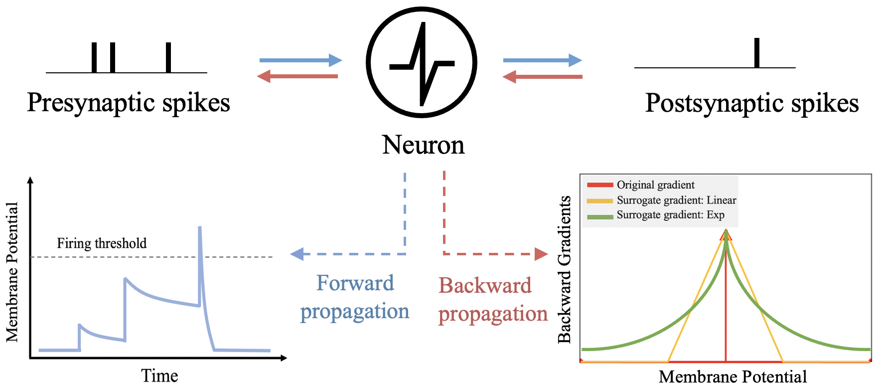
Figure 1: The illustration of forward propagation (blue arrow) and backward propagation (red arrow) of an LIF neuron. During forward propagation, the membrane potential increases according to the pre-synaptic spike input. If the membrane potential exceeds the firing threshold, the LIF neuron generates the post-synaptic spike with the membrane potential reset. This integrate-and-fire behavior induces the non-differentiability of the membrane potential. Therefore, surrogate gradient functions are used to implement the backward gradient.

In this study, we propose a novel visualization tool for SNN, called Spike Activation Map (SAM), which does not require any backpropagation. Instead, we calculate an attention map by monitoring neurons that carry more information (i.e., spikes) over different time-steps during forward propagation. We exploit the biological observation that short Inter-Spike-Interval (ISI) spikes have more information in a neurological system [36, 46, 45] because these spikes are more likely to induce post-synaptic spikes by increasing the membrane potential of the neuron. Specifically, for each neuron, we compute a neuronal contribution score (NCS) for the prediction. The NCS score is defined as the sum of temporal spike contribution score (TSCS) with an exponential kernel. The TSCS score assigns high value for spikes firing within a short time window, otherwise, assigns low value. Then, we add the NCS values across the channel axis to get a 2D spatial heatmap. We highlight that, unlike conventional visualization tools, our SAM does not require target class label to find a contribution or visual explanation [55, 40].

Further, by using SAM, we investigate various configurations of SNNs. Firstly, we compare the internal spiking behavior of two different SNN training methods: surrogate gradient based training [27] and ANN-SNN [41] conversion on a non-trivial image dataset (i.e., Tiny-ImageNet). Then, we observe the spike representation of each layer across different time-steps to understand the temporal characteristics of SNNs. We also analyze the effect of varying factors such as a leak rate and related hyperparameters on SAM and overall prediction. Finally, we provide a visual understanding of previously observed results [43] that SNNs are more robust to adversarial attacks [15]. We measure the difference of heat maps between clean samples and adversarial samples using SAM to highlight the robustness of SNNs with respect to ANNs.

In summary, our key contributions can be summarized as follows: (i) For the first time, we introduce a novel visualization technique for SNNs, called Spike Activation Map (SAM). We circumvent the non-differentiability problem of LIF neuron by calculating an attention map based on short ISI spikes in neurons. (ii) Interestingly, we find that SAM shows reliable visualization results without any ground truth class labels. (iii) By using SAM, we visualize and analyze the temporal characteristics and internal spike behavior of SNNs across various configurations, such as, training schemes, temporal parameters, adversarial inputs. Overall, our proposed SAM opens up the possibility towards interpretable and reliable neuromorphic computing.

2 Related Work

2.1 Spiking Neural Networks

Spiking Neural Networks (SNNs) have recently emerged as the next generation AI due to their huge energy efficiency benefits on asynchronous neuromorphic hardware. Following the recent development of neuromorphic computing architectures such as TrueNorth [3] and Loihi [9], training algorithm of SNNs has received huge attention. One intriguing learning algorithm is spike-timing-dependent plasticity (STDP) [5] with a bio-plausible Hebbian learning rule [18]. This algorithm is based on local learning by using the spike correlation of pre-synaptic spikes and post-synaptic spikes. So far, STDP-based learning has been confined to shallow networks on small-scale datasets due to the absence of a global optimization rule. Another widely-used method is ANN-SNN conversion method [41, 16, 12, 38], which converts a pre-trained ANN to an SNN. Since networks are trained in ANN domain, the training complexity is significantly removed. With careful threshold (or weight) balancing [12], ANN-SNN conversion shows good performance on large-scale datasets. It is worth mentioning that temporal dynamics are not considered in the process of training for converted SNNs. Recently, training SNNs with backpropagation [32, 28, 53, 27] has been studied because it can take into account temporal neuronal dynamics during surrogate gradient descent. Despite the huge progress in training methods for SNNs, there is little attention given to the internal spike behavior of SNNs. Therefore, in this paper, we focus on SNN interpretability. Our results show that surrogate methods which have explicit temporal dependence during training are more interpretable than conversion.

2.2 Visualization Tools for ANNs

The interpretation of prediction in neural networks has received considerable attention due to its practicality in real-world scenarios. Class Activation Map (CAM) [55] highlights the discriminative region of an image by using a global average pooling layer at the end of the feature extractor. The CAM heat map is obtained by summing the feature maps at the last convolutional layer. Several variations of CAM have been proposed [54, 52, 44]. However, the necessity of the global average pooling layer in CAM limits its usage. To address this issue, Selvaraju et al. proposed Grad-CAM [40], which is the generalized version of CAM. Grad-CAM computes backward gradients from the classifier to a given intermediate layer where visual explanation is required. Thus, the contribution of each neuron to the classification result can be quantified with the corresponding gradient value. Then, a 2D heatmap is obtained by using the weighted sum of the activations across the channel axis based on the gradient value. In this work, we justify that directly applying Grad-CAM to calculate visual explanations in SNNs does not yield accurate results due to the non-differentiable nature of LIF neuron as well as non-dependence on temporal dynamics.

3 Background

Poisson Rate Coding: To convert a static image into multiple binary spikes, we use Poisson rate coding, or rate-based coding. This is based on the human visual system [2], and shows outstanding performance among various spike coding schemes such as temporal [31], phase [26], and burst [34]. Poisson coding generates a spike train over multiple time-steps where the number of spikes is approximately proportional to the pixel intensity of the input image. In practice, we compare each pixel value with a random number $[0,255]$ at every time-step. If the generated random number is less than the pixel intensity, the Poisson spike generator does not produce spikes, otherwise, it generates a spike with amplitude $1$. The generated spikes are then passed through an SNN.

Leaky-Integrate-and-Fire Neuron: Leaky-Integrate-and-Fire (LIF) neuron is the main component of SNNs. The internal state of an LIF neuron is represented by a membrane potential $U_{m}$. As time goes on, the membrane potential decays with time constant $\tau_{m}$. Given an input signal $I(t)$ and an input register $R$ at time $t$, the differential equation of the LIF neuron can be formulated as:

$$\tau_{m}\frac{dU_{m}}{dt}=-U_{m}+RI(t).$$ (1)

This continuous dynamic equation is converted into a discrete equation for digital simulation. More concretely, we formulate the membrane potential $u_{i}^{t}$ of a single neuron $i$ as:

$$u_{i}^{t}=\lambda u_{i}^{t-1}+\sum_{j}w_{ij}o^{t}_{j}-\theta o^{t-1}_{i},$$ (2)

where, $\lambda$ is a leak factor, $w_{ij}$ is the weight of the connection between pre-synaptic neuron $j$ and post-synaptic neuron $i$. If the membrane potential $u_{i}^{t-1}$ exceeds a firing threshold $\theta$, the neuron $i$ generate spikes $o_{i}^{t-1}$, which can be formulated as:

$$o^{t-1}_{i}=\begin{cases}1,&\text{if $u_{i}^{t-1}>\theta$},\\ 0&\text{otherwise.}\end{cases}$$ (3)

After the neuron fires, we perform a soft reset, where the membrane potential value is lowered by threshold $\theta$. Because of this non-differentiable firing behavior, training SNNs with gradient learning is a huge challenge [37]. To address this issue, previous studies [32, 28] approximate the backward gradient function (e.g., piecewise linear and exponential) to implement gradient learning. Fig. 1 illustrates the membrane potential dynamics of an LIF neuron.

4 Methodology

In this paper, we visualize the internal spike behavior of two representative and widely-used training methods: surrogate gradient training [27] and ANN-SNN conversion [41]. Since ANNs can be trained with well-established optimization methods and frameworks, SNNs from ANN-SNN conversion shows reliable performance on very large-scale datasets (e.g., ImageNet). In contrast, most surrogate gradient training methods are limited to small datasets (e.g., MNIST and CIFAR10) due to approximated backward gradients. These simple datasets are too small to be analyzed by visualizing heatmap. But, the authors in [27] recently proposed temporal adaptive batch normalization (BN) for surrogate gradient learning, enabling training on larger datasets such as CIFAR100 and Tiny-ImageNet. We exploit this algorithm for the case study of surrogate gradient training to compare with ANN-SNN conversion on Tiny-ImageNet dataset.

4.1 Surrogate Gradient Backpropagation

The SNN-crafted BN layer [27], called Batch Normalization Through Time (BNTT), improves training stability and reduces latency while preserving classification accuracy. We add the BNTT layer before an LIF neuron. Therefore, the weighted pre-synaptic input spikes are normalized as:

$$u_{i}^{t}=\lambda u_{i}^{t-1}+\gamma_{i}^{t}(\frac{\sum_{j}w_{ij}o^{t}_{j}-\mu^{t}_{i}}{\sqrt{(\sigma_{i}^{t})^{2}+\epsilon}})-\theta o^{t-1}_{i},$$ (4)

where, $\gamma_{i}^{t}$ is a learnable parameter in the BNTT layer, $\epsilon$ is a small constant for numerical stability, the mean $\mu_{i}^{t}$ and variance $\sigma_{i}^{t}$ are calculated from the samples in a mini-batch for each time step $t$. We append all intermediate layers of an SNN with a BNTT layer. At the output layer, we set the number of output neurons to the number of classes $C$. To prevent information loss from the leakage of a neuron, we accumulate the spikes over all time-steps by fixing the leak parameter $\lambda$ (Eq. 2) as one. This stacked voltage is converted into probability distribution using a softmax layer. Finally, we compute the cross-entropy loss as:

$${L}=-\sum_{i}y_{i}log(\frac{e^{u_{i}^{T}}}{\sum_{k=1}^{C}e^{u_{k}^{T}}}).\vspace{-2mm}$$ (5)

Here, $y_{i}$ represents the ground truth label, and $T$ is the total number of time-steps.

Then, we accumulate the backward gradients over all time-steps, which is called back-propagation through time (BPTT) [32]. The accumulated gradients at hidden layers and the output layer can be represented as:

$$\Delta W_{l}=\sum_{t}\frac{\partial L}{\partial W_{l}^{t}}=\begin{cases}\sum_{t}\frac{\partial L}{\partial O_{l}^{t}}\frac{\partial O_{l}^{t}}{\partial U_{l}^{t}}\frac{\partial U_{l}^{t}}{\partial W_{l}^{t}},&\text{$l$: hidden layer}\\ \sum_{t}\frac{\partial L}{\partial U_{l}^{T}}\frac{\partial U_{l}^{T}}{\partial W_{l}^{t}},&\text{$l$: output layer}\end{cases}\vspace{-1mm}$$ (6)

where, $W_{l}$, $O_{l}$ and $U_{l}$ stand for weight matrix, output spike matrix, and membrane potential matrix at layer $l$, respectively. As the output layer does not generate spikes, we compute the exact derivative of the loss $L$ with respect to the membrane potential $u_{i}^{T}$:

$$\frac{\partial L}{\partial u_{i}^{T}}=\frac{e^{u_{i}^{T}}}{\sum_{k=1}^{C}e^{u_{k}^{T}}}-y_{i}.\vspace{-2mm}$$ (7)

However, for hidden layer, the gradient term $\frac{\partial o_{i}^{t}}{\partial u_{i}^{t}}$ is not differentiable due to the firing behavior of an LIF neuron. Therefore, $\frac{\partial o_{i}^{t}}{\partial u_{i}^{t}}$ should be formulated with an approximated continuous function (Fig. 1). To this end, we use a piecewise linear function:

$$\frac{\partial o_{i}^{t}}{\partial u_{i}^{t}}=\beta\max\{0,1-\ |\frac{u_{i}^{t}-\theta}{\theta}\ |\},\vspace{-1mm}$$ (8)

where, $\beta$ is a scaling factor for the gradient value. We set $\beta$ as 0.3 to prevent a gradient exploding problem. Based on the gradient value, the weights of SNNs are updated.

Algorithm 1 ANN-SNN Conversion

Input: Input set ($X$); label set ($Y$); max_timestep ($T$); pre-trained ANN model (A); SNN model (S); total layer number (L)
Output: Updated SNN network with threshold balancing

1:// Copy ANN weights to SNN

2:$S.weights\leftarrow A.weights$

3:// Initialize threshold voltage

4:$S.th$ $\leftarrow$ 0

5:for $l\leftarrow 1$ to $L-1$ do

6:    for $t\leftarrow 1$ to $T$ do

7:         $O^{t}$ $\leftarrow$ PoissonGenerator(X)

8:         for $l_{tmp}\leftarrow 1$ to $l$ do

9:             if $l_{tmp}<l$ then

10:                 $(O^{t}_{l},U_{l}^{t})\leftarrow(U_{l}^{t-1},W_{l},O^{t-1}_{l-1})$

11:             else

12:                 // Threshold update for each layer

13:                 $S_{l}.th$ $\leftarrow$ max($S_{l}.th$, ${W_{l}O^{t-1}_{l-1}}$)

14:             end if

15:         end for

16:    end for

17:end for

4.2 ANN-SNN Conversion

We use [41] for implementing the ANN-SNN conversion method. They normalize the weights or the firing threshold ($\theta$ in Eq. 3) to take into account the actual SNN operation in the conversion process. The overall algorithm for the conversion method is shown in Algorithm 1. First, we copy the weight parameters of a pre-trained ANN to an SNN. Then, for every layer, we compute the maximum activation across all time-steps and set the firing threshold to the maximum activation value. The conversion process starts from the first layer and sequentially goes through deeper layers. Note that we do not use BN [22] since all input spikes have zero mean values.Also, following the previous works [16, 41, 12], we use Dropout [47] for both ANNs and SNNs.

4.3 SNN-crafted Grad-CAM

Grad-CAM [40] highlights the region of the image that highly contributes to classification results. Grad-CAM computes a backward gradient from the classifier logit to the pre-defined target layer. After that, channel-wise attention value is obtained by using global average pooling. Based on this, the final heatmap is defined as the weighted sum of feature maps. Different from conventional deep neural networks, SNNs take spike trains across multiple time-steps. Therefore, we can compute multiple SNN-crafted Grad-CAMs across the total number of time-steps $T$. Similar to Grad-CAM, we quantify the contribution of each channel by accumulating gradients across all time-steps:

$$\alpha^{c,k}=\frac{1}{N}\sum_{i}\sum_{j}\sum_{t}\frac{\partial y^{c}}{\partial A^{k}_{ij,t}}.$$ (9)

Here, $N$ is a normalization factor, and $A^{k}_{ij,t}$ is the activation value of the $k$th channel at time-step $t$, and (i, j) is the pixel location. Note that we use a ground truth label $c$ for a given image to compute the heatmap. Therefore, the channel-wise weighted sum of spike activation can be calculated as:

$$G^{c}_{ij,t}=max(0,\sum_{k}\alpha^{c,k}_{t}A^{k}_{ij,t}).$$ (10)

For a clear comparison with conventional Grad-CAM, we call $G^{c}_{ij,t}$ as “SNN-crafted Grad-CAM” afterward.

However, SNN-crafted Grad-CAM suffers from what we term as a “heatmap smoothing effect” caused by the approximated backward gradient function. To visualize the heatmap at shallow/initial layers, the gradients need to pass through multiple layers using the approximated backward function (Eq. 8). The accumulated approximation error induces non-discriminative heatmap as shown in Fig. 2. Note that the beginning and end of time-steps have few spike activity [27] resulting in heatmaps with zero values (see Fig. 2). To validate the “heatmap smoothing effect” quantitatively, we compute the pixel-wise variance of the heatmap. Thus, the heatmap containing non-discriminative information (i.e. similar pixel values) should have lower variance. In Fig. 3, SNN-crafted Grad-CAM shows lower variance compared to our proposed SAM (will be discussed in the next section). Note that there are multiple heatmaps (one heatmap per time-step) in SNN visualization. So, we use the maximum variance value across all time-steps in Fig. 3. Further, we note that the visualization in both SAM and SNN-crafted Grad-CAM in Fig. 2 varies across each time-step underlying the fact that the SNN looks at different regions of the same input over time to make a prediction. Overall, the visualization tool for SNNs requires a new perspective that can circumvent the error accumulation problem in backpropagation.

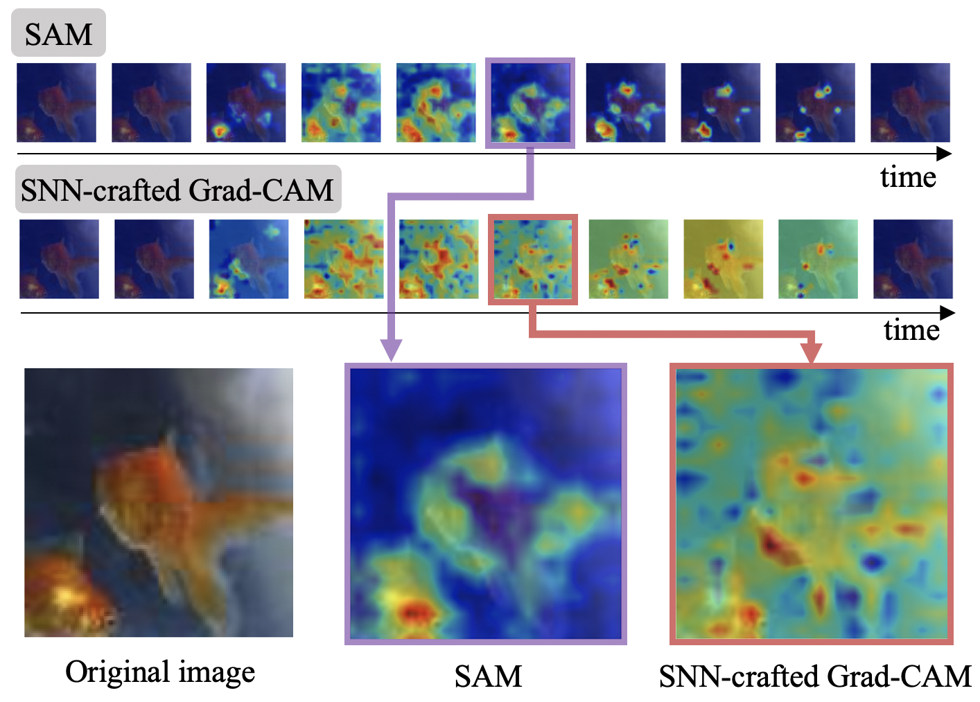
Figure 2: Visualization of SNN-crafted Grad-CAM and SAM at Conv4 in VGG11 on Tiny-ImageNet dataset. We use surrogate gradient training (the conversion method also shows similar results). The approximated backward gradient function in SNN-crafted Grad-CAM induces “heatmap smoothing effect”. In contrast, the proposed SAM visualization highlights the discriminative region of the image.

4.4 Spike Activation Map (SAM)

We present a new paradigm for the visualization of SNNs. We do not use any class label for backpropagation, and only use the spike activity in forward propagation. Thus, this heatmap is not just for a specific class but highlights the regions that the network focuses for any given image. Surprisingly, we observe that SAM shows meaningful visualization even without any ground truth labels (see Section 5.2). Mathematically, our objective can be formulated as to find a mapping function $f(\cdot)$:

$$M_{t}\leftarrow f(S_{0},S_{1},...,S_{t-1}),$$ (11)

where, $M_{t}$ is SAM and $S_{t}$ is spike activity at time-step $t$. In this paper, we use the biological observation that spikes having short inter-spike interval (ISI) highly contribute to the neural decision process [36, 46, 45]. This is because short-ISI spikes are more likely to stimulate post-synaptic neurons, conveying more information [4, 30, 46]. To apply this to our visualization method, we first define the temporal spike contribution score (TSCS) which evaluates the contribution of previous spike at time $t^{\prime}$ to the current time $t$ in the same neuron. The TSCS value can be formulated as:

$$T(t,t^{\prime})=\exp(-\gamma|t-t^{\prime}|),$$ (12)

where, $\gamma$ is a hyperparameter which controls the steepness of the exponential kernel function.

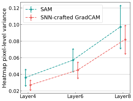
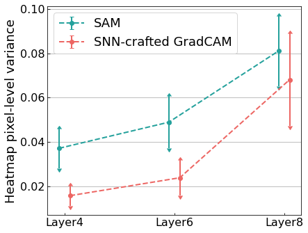
(a) Surrogate Gradient	(b) Conversion

Figure 3: Pixel-level variance in heatmaps obtained from surrogate gradient learning and conversion. We report the average variance from the total samples in Tiny-ImageNet. For all scenarios, SAM shows a higher hearmap variance compared to SNN-crafted Grad-CAM that suffers from the approximated backward gradient.

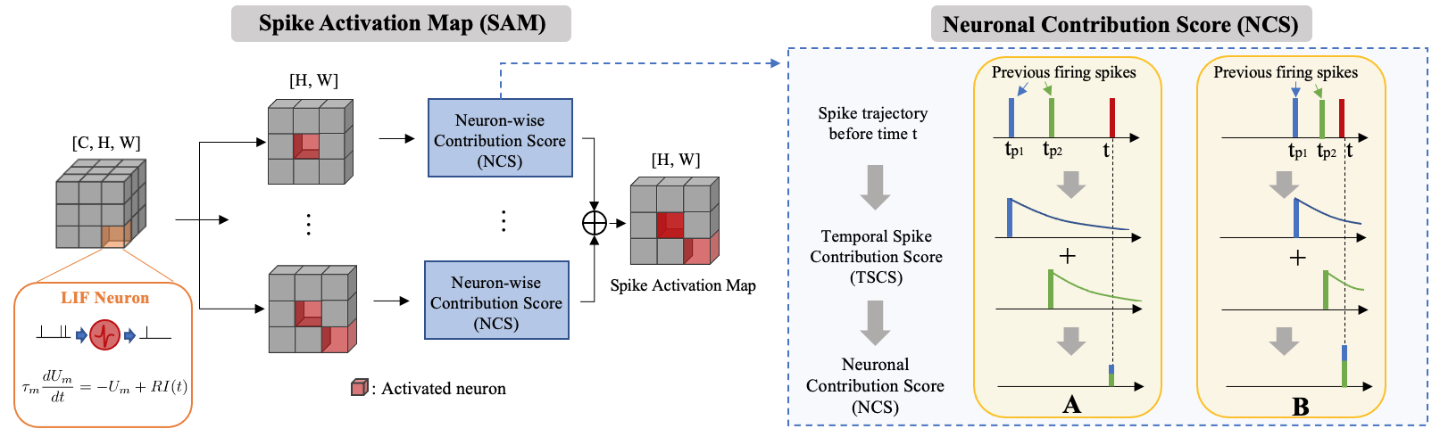
Figure 4: Illustration of spike activation map (SAM). For each channel, we compute a neuron-wise contribution score. After that, we sum all neuronal contribution score (NCS) map in the channel axis. The NCS for each neuron is based on the previous spike trajectory. For every spike, we define temporal spike contribution score (TSCS) with an exponential kernel. We take into account TSCS from previous spikes in order to compute NCS.

To consider multiple previous spikes, we define a set $P_{ij}^{k}$ that consists of previous firing times of a neuron at location $(i,j)$ in $k$th channel. For every time-step, we compute a neuronal contribution score (NCS) $N^{k}_{ij,t}$ at time-step $t$, by adding all TSCS of spikes in $P_{ij}^{k}$:

$$N^{k}_{ij,t}=\sum_{t^{\prime}\in P_{ij}^{k}}T(t,t^{\prime}).$$ (13)

Thus, a neuron has a high NCS if large number of spikes are fired in a short time interval and vice-versa. Finally, we calculate the SAM heatmap $M_{ij,t}$ at time-step $t$ and location $(i,j)$ by multiplying spike activity $S_{ij,t}$ with NCS value $N_{ij,t}$:

$$M_{ij,t}=\sum_{k}N_{ij,t}^{k}S^{k}_{ij,t}.$$ (14)

We illustrate the overall flow of SAM in Fig. 4. For every neuron, we compute NCS and add the values across the channel axis in order to get SAM. To elaborate, we depict two examples (case A and case B) for calculating NCS. In case $A$, the previous spikes fire at time-step $t_{p1}$ and $t_{p2}$, a long time before the current spike time $t$. As a result, the contribution of previous spikes is small due to the exponential kernel. On the other hand, in case $B$, $t_{p1}$ and $t_{p2}$ are close to the current spike time $t$. In this case, the neuron has a high NCS value.

Discussion: Overall, without any requirement for backpropagation and ground truth labels, we can visualize the discriminative region by using the concept of inter-spike interval. We would like to note that SAM cannot be applied to ANNs due to the real-valued static nature of input processing in ANNs. So far, SNNs have been explored as an energy-efficient alternative to ANNs. With SAM, for the first time, we bring out the interpretability advantage of the temporal dynamics in SNNs over static ANNs. We assert that the proposed SAM is hardware friendly since all computations are in forward propagation. Therefore, our SAM can be used as a practical interpretation tool for future neuromorphic computing applications.

5 Experiments

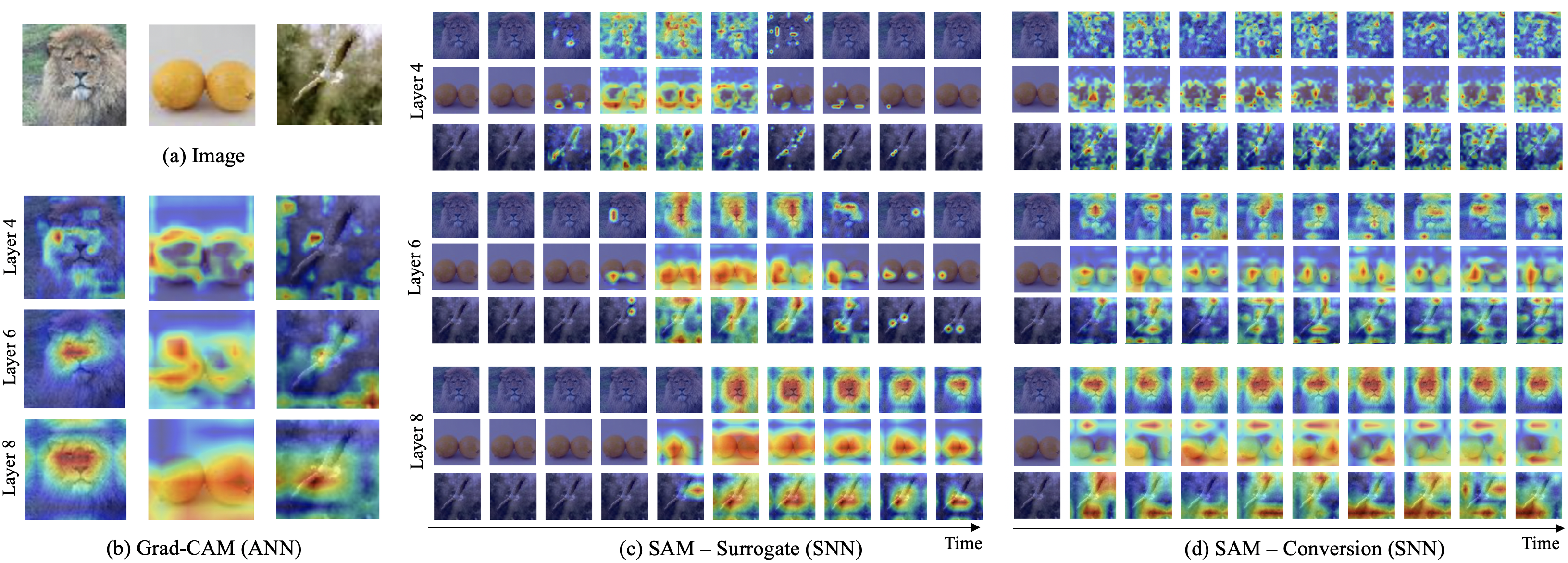
Figure 5: Visualization of the internal spike representation of VGG11 using SAM at layer 4, layer 6, and layer 8. We show the visualization for 10 uniformly sampled time-steps. It is worth mentioning Grad-CAM exploits ground truth labels but our SAM can be obtained without any label information.

5.1 Experimental Setup

Dataset and Network: To conduct a comprehensive analysis, we carefully select the dataset for our experiments. This is because smaller datasets such as MNIST, CIFAR10, and CIFAR100 have too low resolution (e.g., $28\times 28$ or $32\times 32$) to visualize. ImageNet dataset has a high image resolution but directly training SNNs with surrogate gradient becomes hard. Therefore, we conduct a case study on the Tiny-ImageNet which is the modified subset of the original ImageNet dataset. Tiny-ImageNet consists of 200 different classes of ImageNet dataset [10], with 100,000 training and 10,000 validation images. The resolution of the images is $64\times 64$ pixels. Our implementation is based on Pytorch [35]. We adopt a VGG11 architecture for both ANNs and SNNs. For ANN-SNN conversion method, we use 500 time-steps with firing threshold scaling [16]. For surrogate gradient training, we train the networks with standard SGD with momentum 0.9, weight decay 0.0005, time-steps 30. The base learning rate is set to 0.1. We use step-wise learning rate scheduling with a decay factor 10 at [0.5, 0.7, 0.9] of the total number of epochs. We set the total number of epochs to 90. We set the leak factor of SNN with surrogate gradient learning and conversion to 0.99 and 1, respectively. For visualization, we uniformly sample 10 images for both surrogate gradient learning and conversion.

Evaluation Metric: To quantitatively compare the SAM visualization of conversion and surrogate gradient, we use Grad-CAM obtained from ANNs as a reference. To quantify the error between SAM and Grad-CAM, we compute the cross entropy function between the predicted SAMs (one SAM for one time-step) and a Grad-CAM from ANN at every time-step. Then we select the minimum error across all time-steps and define the minimum value as a localization error.

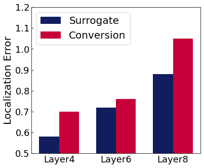
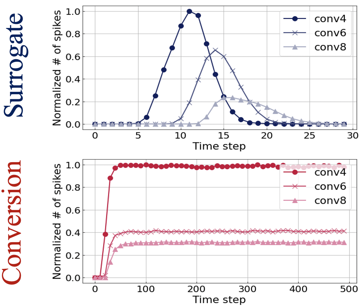
(a)	(b)

Figure 6: (a) Localization error comparison. We compare SAM from surrogate gradient learning and conversion with Grad-CAM. (b) Visualization of the normalized number of spikes.

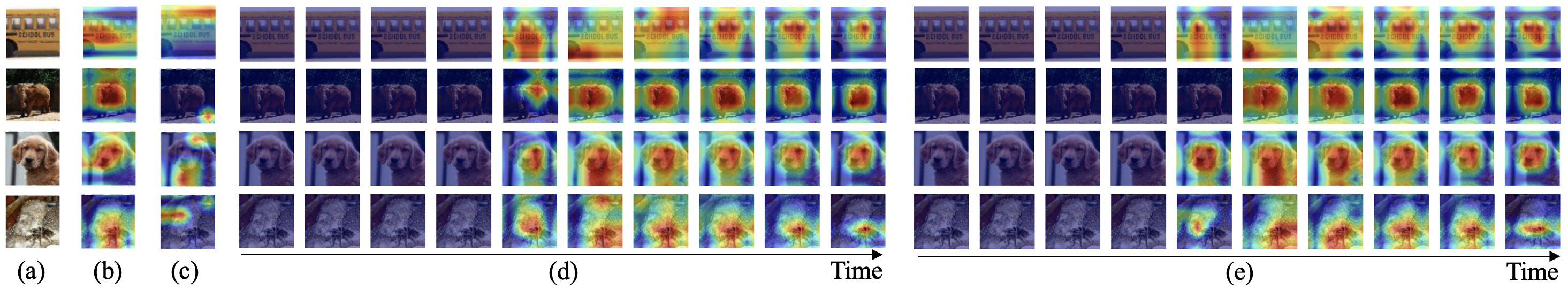
Figure 7: Visualization of robustness of SAM. (a) Original image. (b) Grad-CAM from ANN on clean input. (c) Grad-CAM from ANN on adversarial input. SAM from SNN trained with surrogate gradient learning on (d) clean inputs and (e) adversarial inputs.

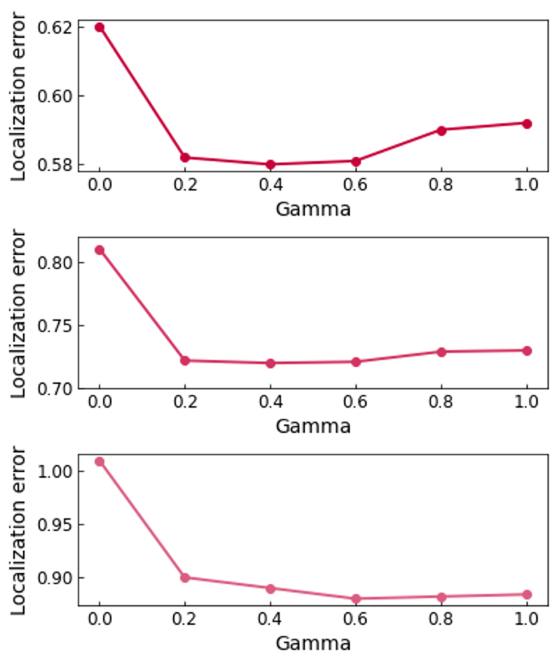
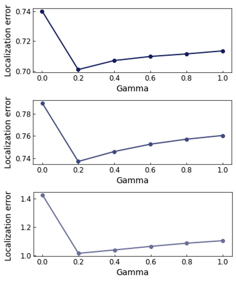
(a) Surrogate Gradient	(b) Conversion

Figure 8: Localization error at layer 4 (top row), layer 6 (middle row), and layer 8 (bottom row) with respect to hyperparameter $\gamma$.

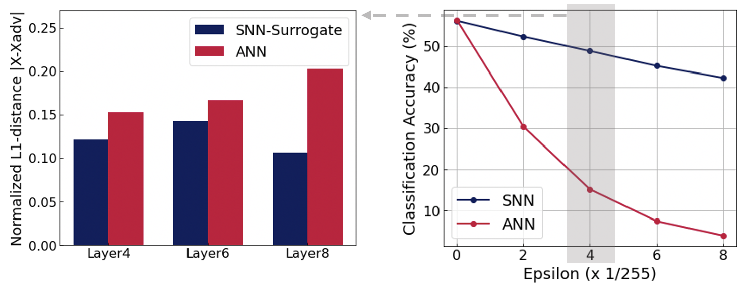
Figure 9: Classification accuracy with respect to the FGSM intensity. We also compute the normalized L1 distance between heatmaps for clean and adversarial inputs at $\epsilon=\frac{4}{255}$. For SNN, we report the maximum difference among multiple time-steps.

5.2 SAM: Unsupervised Visualization Tool

In Fig. 5, we visualize the qualitative results of SAM on SNNs trained with surrogate learning as well as ANN-SNN conversion. We also show the Grad-CAM visualization obtained from a corresponding ANN for reference. Note that SAM does not require any class label (unsupervised) compared to Grad-CAM that uses ground truth class labels. Interestingly, heatmaps obtained from SAM across different time-steps on SNNs shows a similar result with Grad-CAM on ANNs where the region of interest is highlighted in a discriminative fashion. This supports our assertion that SAM is an effective visualization tool for SNNs. Moreover, the results imply that ISI and temporal dynamics can yield intepretability for deep SNNs.

5.3 Surrogate Gradient Learning vs. Conversion

We compare the SAM visualization results of surrogate gradient learning (Fig. 5(c)) and conversion (Fig. 5(d)). From the figure, we observe a trend in the heatmap visualization of surrogate gradient learning with zero activity at early time-steps leading to discriminative activity in the mid-range followed by zero activity again towards the end. In contrast, conversion maintains similar heatmaps during the entire time period. This is related to the variation in spike activity for each time-step as shown in Fig. 6(b). Since surrogate gradient learning considers a temporal dynamic during training [27, 37], each layer passes the information (i.e., the number of spikes) consecutively. On the other hand, conversion does not show any temporal propagation. Moreover, we observe that surrogate gradient learning has more accurate (i.e. similar to Grad-CAM from ANN) heatmaps highlighting the region of interest across all layers. Notably, the conversion method highlights only partial regions of the object (e.g., lemon) and in some cases (e.g., bird) the wrong region. This observation is supported by the localization error comparison in Fig. 6(a). For all layers, surrogate gradient learning shows lower localization error. It is well known and evident that conversion methods do not account for any temporal dynamics during training [37]. We believe that this missing temporal dependence accounts for less interpretability. Thus, we assert that SNNs obtained with surrogate gradient learning (incorporating temporal dynamics) are more interpretable. Therefore, all visualization analyses in the next sections focus on the surrogate gradient learning method.

5.4 Intermediate Layers of SNN

So far, no studies have analysed the underlying information learnt in different layers of an SNN. It has been always assumed that SNNs like ANNs learn features in a generic-to-specific manner as we go deeper. For the first time, we visualize the explanations at intermediate layers of SNN using SAM to support this assumption. In Fig. 5 (see SAM-Surrogate results), the SAM visualization shows that shallow layers of SNNs represent low-level structure and deep layers focus on semantic information. For example, layer 4 highlights the edges or blobs of the lion, such as eyes and nose. On the other hand, layer 8 highlights the full face of the lion.

Table 1: Ablation studies on leak factor $\lambda$. We show localization error and classification accuracy with respect to $\lambda$.

	$\lambda=0.7$	$\lambda=0.8$	$\lambda=0.9$
Localization Error (Layer 4)	0.68	0.63	0.61
Localization Error (Layer 6)	0.86	0.82	0.80
Localization Error (Layer 8)	0.98	0.97	0.91
Accuracy (%)	47.53	53.36	56.57

5.5 Effect of Leak in SNN

We analyze the effect of leak factor $\lambda$ (Eq. 2), one of the important parameters in SNNs. The leak parameter $\lambda$ ($0<\lambda\leq 1$) controls the forgetting behavior of LIF neurons similar to the human brain. We note that high $\lambda$ means less forgetting. In order to explain the effect of leak on visualization, we measure the localization error for different leak values [0.7, 0.8, 0.9]. Table 1 shows that high leak parameter $\lambda$ achieves low localization error. This is because a low $\lambda$ forgets the stored voltage in a neuron (i.e. information) within a few time-steps and thus cannot produce any reasinable spike activity or visualization. We also compute the classification accuracy on Tiny-ImageNet in Table 1. The results show that low $\lambda$ induces a drastic accuracy drop due to the excessive forgetting behavior. Overall, appropriate leak selection is important to achieve accurate localization/visualization as well as performance.

5.6 Effect of Hyperparamter $\gamma$

We conduct ablation studies to understand the effect of hyperparameter $\gamma$ on SAM in Eq. 12. The $\gamma$ value decides the steepness of the exponential kernel function in TSCS. A kernel with high $\gamma$ takes into account recent spike trajectory, where as low $\gamma$ considers long-period spike trajectory. In Fig. 8, we visualize the localization error with respect to $\gamma$ for different layers in VGG 11 for conversion and surrogate gradient methods. For both methods, $\gamma=0$ shows the highest localization error since the kernel does not filter redundant long ISI spikes. Another interesting observation is that the localization error increases for large gamma value (e.g., 1.0). This is because high $\gamma$ limits reliable visualization by considering only very recent spikes and ignores spike history to a great extent.

5.7 Adversarial Robustness of SNN

Previous studies [43, 42] have shown that SNNs are more robust to adversarial inputs than ANNs. In order to observe the effectiveness of SNNs under attack, we conduct a qualitative and quantitative comparison between Grad-CAM and SAM. We attack both ANN and SNN using FGSM attack [15] and SNN-crafted FGSM attack [43] with $\epsilon=\frac{4}{255}$. In Fig. 7, we can observe that Grad-CAM shows large change before/after attack. On the other hand, SAM shows almost similar results. Moreover, we show the classification accuracy with respect to the attack intensity, and normalized L1-distance between heatmaps of clean and adversarial images at $\epsilon=\frac{4}{255}$, in Fig. 9. The results show that SNN is more robust than ANN in terms of both accuracy and visualization. Therefore, using SNN with SAM for a secured system (e.g., military defense) will be a huge advantage in terms of robust interpretation.

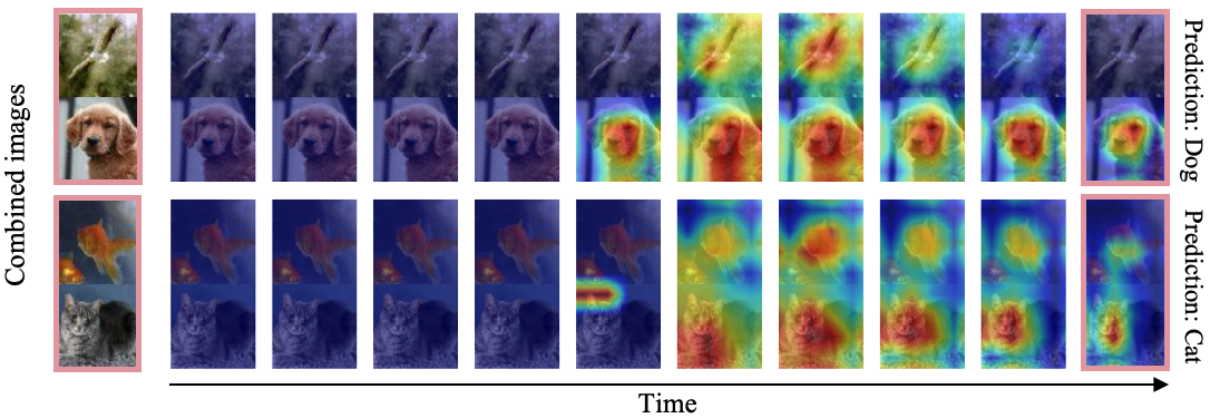
Figure 10: Visualization of SAM for multi-object images.

5.8 Sensory Suppression Behavior of SNN

Neuroscience studies have suggested that human brain undergoes [24, 25, 50] “sensory suppression”. That is, the brain focuses on one of multiple objects when these objects are presented at the same time. Co-incidentally, with SAM, we observe that SNNs also emulate sensory suppression when presented with multiple objects. To show this, we concatenate two randomly chosen images from Tiny ImageNet dataset and pass the concatenated image into the SNN trained with surrogate gradient learning. Interestingly, as shown in Fig. 10, the results show that neurons compete in the earlier time-steps for attending to both objects and finally focus/attend on only one of the objects at later time-steps. Note, for each image, the final prediction from the SNN matches the final attention shown by SAM. These results unleash the bio-plausible characteristics of SNNs and also establish SAM as a suitable interpretation tool.

6 Conclusion

In this paper, we propose a visualization tool for SNNs, called SAM. This is different from a conventional ANN visualization tool since SAM does not require any target labels and backpropagated gradients. Instead, we use the temporal dynamics of SNNs to compute a neuronal contribution score in forward propagation based on the history of previous spikes. Without any label, SAM highlight the discriminative region for prediction. Through extensive experiments, we show the functionality of SAM in various configuration of SNNs. Overall, SAM opens up the possibility towards interpretable neuromorphic computing.

7 Acknowledgement

The research was funded in part by C-BRIC, one of six centers in JUMP, a Semiconductor Research Corporation (SRC) program sponsored by DARPA, the National Science Foundation (Grant#1947826), and the Amazon Research Award.

References

- [1] Martín Abadi, Ashish Agarwal, Paul Barham, Eugene Brevdo, Zhifeng Chen, Craig Citro, Greg S Corrado, Andy Davis, Jeffrey Dean, Matthieu Devin, et al. Tensorflow: Large-scale machine learning on heterogeneous distributed systems. arXiv preprint arXiv:1603.04467, 2016.
- [2] Edgar D Adrian and Yngve Zotterman. The impulses produced by sensory nerve-endings: Part ii. the response of a single end-organ. The Journal of physiology, 61(2):151, 1926.
- [3] Filipp Akopyan, Jun Sawada, Andrew Cassidy, Rodrigo Alvarez-Icaza, John Arthur, Paul Merolla, Nabil Imam, Yutaka Nakamura, Pallab Datta, Gi-Joon Nam, et al. Truenorth: Design and tool flow of a 65 mw 1 million neuron programmable neurosynaptic chip. IEEE transactions on computer-aided design of integrated circuits and systems, 34(10):1537–1557, 2015.
- [4] Jose-Manuel Alonso, W Martin Usrey, and R Clay Reid. Precisely correlated firing in cells of the lateral geniculate nucleus. Nature, 383(6603):815–819, 1996.
- [5] Guo-qiang Bi and Mu-ming Poo. Synaptic modifications in cultured hippocampal neurons: dependence on spike timing, synaptic strength, and postsynaptic cell type. Journal of neuroscience, 18(24):10464–10472, 1998.
- [6] Zhenshan Bing, Claus Meschede, Florian Röhrbein, Kai Huang, and Alois C Knoll. A survey of robotics control based on learning-inspired spiking neural networks. Frontiers in neurorobotics, 12:35, 2018.
- [7] Yongqiang Cao, Yang Chen, and Deepak Khosla. Spiking deep convolutional neural networks for energy-efficient object recognition. International Journal of Computer Vision, 113(1):54–66, 2015.
- [8] Iulia M Comsa, Thomas Fischbacher, Krzysztof Potempa, Andrea Gesmundo, Luca Versari, and Jyrki Alakuijala. Temporal coding in spiking neural networks with alpha synaptic function. In ICASSP 2020-2020 IEEE International Conference on Acoustics, Speech and Signal Processing (ICASSP), pages 8529–8533. IEEE, 2020.
- [9] Mike Davies, Narayan Srinivasa, Tsung-Han Lin, Gautham Chinya, Yongqiang Cao, Sri Harsha Choday, Georgios Dimou, Prasad Joshi, Nabil Imam, Shweta Jain, et al. Loihi: A neuromorphic manycore processor with on-chip learning. IEEE Micro, 38(1):82–99, 2018.
- [10] Jia Deng, Wei Dong, Richard Socher, Li-Jia Li, Kai Li, and Li Fei-Fei. Imagenet: A large-scale hierarchical image database. In 2009 IEEE conference on computer vision and pattern recognition, pages 248–255. Ieee, 2009.
- [11] Peter U Diehl and Matthew Cook. Unsupervised learning of digit recognition using spike-timing-dependent plasticity. Frontiers in computational neuroscience, 9:99, 2015.
- [12] Peter U Diehl, Daniel Neil, Jonathan Binas, Matthew Cook, Shih-Chii Liu, and Michael Pfeiffer. Fast-classifying, high-accuracy spiking deep networks through weight and threshold balancing. In 2015 International Joint Conference on Neural Networks (IJCNN), pages 1–8. ieee, 2015.
- [13] Alexey Dosovitskiy and Thomas Brox. Inverting visual representations with convolutional networks. In Proceedings of the IEEE conference on computer vision and pattern recognition, pages 4829–4837, 2016.
- [14] Steve B Furber, Francesco Galluppi, Steve Temple, and Luis A Plana. The spinnaker project. Proceedings of the IEEE, 102(5):652–665, 2014.
- [15] Ian J Goodfellow, Jonathon Shlens, and Christian Szegedy. Explaining and harnessing adversarial examples. arXiv preprint arXiv:1412.6572, 2014.
- [16] Bing Han, Gopalakrishnan Srinivasan, and Kaushik Roy. Rmp-snn: Residual membrane potential neuron for enabling deeper high-accuracy and low-latency spiking neural network. In Proceedings of the IEEE/CVF Conference on Computer Vision and Pattern Recognition, pages 13558–13567, 2020.
- [17] Kaiming He, Xiangyu Zhang, Shaoqing Ren, and Jian Sun. Deep residual learning for image recognition. In Proceedings of the IEEE conference on computer vision and pattern recognition, pages 770–778, 2016.
- [18] Donald Olding Hebb. The organization of behavior: A neuropsychological theory. Psychology Press, 2005.
- [19] Fred Hohman, Minsuk Kahng, Robert Pienta, and Duen Horng Chau. Visual analytics in deep learning: An interrogative survey for the next frontiers. IEEE transactions on visualization and computer graphics, 25(8):2674–2693, 2018.
- [20] Tiffany Hwu, Jacob Isbell, Nicolas Oros, and Jeffrey Krichmar. A self-driving robot using deep convolutional neural networks on neuromorphic hardware. In 2017 International Joint Conference on Neural Networks (IJCNN), pages 635–641. IEEE, 2017.
- [21] Forrest N Iandola, Song Han, Matthew W Moskewicz, Khalid Ashraf, William J Dally, and Kurt Keutzer. Squeezenet: Alexnet-level accuracy with 50x fewer parameters and¡ 0.5 mb model size. arXiv preprint arXiv:1602.07360, 2016.
- [22] Sergey Ioffe and Christian Szegedy. Batch normalization: Accelerating deep network training by reducing internal covariate shift. arXiv preprint arXiv:1502.03167, 2015.
- [23] Eugene M Izhikevich. Simple model of spiking neurons. IEEE Transactions on neural networks, 14(6):1569–1572, 2003.
- [24] Sabine Kastner, Peter De Weerd, Robert Desimone, and Leslie G Ungerleider. Mechanisms of directed attention in the human extrastriate cortex as revealed by functional mri. science, 282(5386):108–111, 1998.
- [25] Sabine Kastner and Leslie G Ungerleider. The neural basis of biased competition in human visual cortex. Neuropsychologia, 39(12):1263–1276, 2001.
- [26] Jaehyun Kim, Heesu Kim, Subin Huh, Jinho Lee, and Kiyoung Choi. Deep neural networks with weighted spikes. Neurocomputing, 311:373–386, 2018.
- [27] Youngeun Kim and Priyadarshini Panda. Revisiting batch normalization for training low-latency deep spiking neural networks from scratch. arXiv preprint arXiv:2010.01729, 2020.
- [28] Chankyu Lee, Syed Shakib Sarwar, Priyadarshini Panda, Gopalakrishnan Srinivasan, and Kaushik Roy. Enabling spike-based backpropagation for training deep neural network architectures. Frontiers in Neuroscience, 14, 2020.
- [29] Jun Haeng Lee, Tobi Delbruck, and Michael Pfeiffer. Training deep spiking neural networks using backpropagation. Frontiers in neuroscience, 10:508, 2016.
- [30] John E Lisman. Bursts as a unit of neural information: making unreliable synapses reliable. Trends in neurosciences, 20(1):38–43, 1997.
- [31] Hesham Mostafa. Supervised learning based on temporal coding in spiking neural networks. IEEE transactions on neural networks and learning systems, 29(7):3227–3235, 2017.
- [32] Emre O Neftci, Hesham Mostafa, and Friedemann Zenke. Surrogate gradient learning in spiking neural networks. IEEE Signal Processing Magazine, 36:61–63, 2019.
- [33] Priyadarshini Panda, Sai Aparna Aketi, and Kaushik Roy. Toward scalable, efficient, and accurate deep spiking neural networks with backward residual connections, stochastic softmax, and hybridization. Frontiers in Neuroscience, 14, 2020.
- [34] Seongsik Park, Seijoon Kim, Hyeokjun Choe, and Sungroh Yoon. Fast and efficient information transmission with burst spikes in deep spiking neural networks. In 2019 56th ACM/IEEE Design Automation Conference (DAC), pages 1–6. IEEE, 2019.
- [35] Adam Paszke, Sam Gross, Soumith Chintala, Gregory Chanan, Edward Yang, Zachary DeVito, Zeming Lin, Alban Desmaison, Luca Antiga, and Adam Lerer. Automatic differentiation in pytorch. In NIPS-W, 2017.
- [36] Daniel S Reich, Ferenc Mechler, Keith P Purpura, and Jonathan D Victor. Interspike intervals, receptive fields, and information encoding in primary visual cortex. Journal of Neuroscience, 20(5):1964–1974, 2000.
- [37] Kaushik Roy, Akhilesh Jaiswal, and Priyadarshini Panda. Towards spike-based machine intelligence with neuromorphic computing. Nature, 575(7784):607–617, 2019.
- [38] Bodo Rueckauer, Iulia-Alexandra Lungu, Yuhuang Hu, Michael Pfeiffer, and Shih-Chii Liu. Conversion of continuous-valued deep networks to efficient event-driven networks for image classification. Frontiers in neuroscience, 11:682, 2017.
- [39] Llewyn Salt, David Howard, Giacomo Indiveri, and Yulia Sandamirskaya. Parameter optimization and learning in a spiking neural network for uav obstacle avoidance targeting neuromorphic processors. IEEE Transactions on Neural Networks and Learning Systems, 2019.
- [40] Ramprasaath R Selvaraju, Michael Cogswell, Abhishek Das, Ramakrishna Vedantam, Devi Parikh, and Dhruv Batra. Grad-cam: Visual explanations from deep networks via gradient-based localization. In Proceedings of the IEEE international conference on computer vision, pages 618–626, 2017.
- [41] Abhronil Sengupta, Yuting Ye, Robert Wang, Chiao Liu, and Kaushik Roy. Going deeper in spiking neural networks: Vgg and residual architectures. Frontiers in neuroscience, 13:95, 2019.
- [42] Saima Sharmin, Priyadarshini Panda, Syed Shakib Sarwar, Chankyu Lee, Wachirawit Ponghiran, and Kaushik Roy. A comprehensive analysis on adversarial robustness of spiking neural networks. In 2019 International Joint Conference on Neural Networks (IJCNN), pages 1–8. IEEE, 2019.
- [43] Saima Sharmin, Nitin Rathi, Priyadarshini Panda, and Kaushik Roy. Inherent adversarial robustness of deep spiking neural networks: Effects of discrete input encoding and non-linear activations. arXiv preprint arXiv:2003.10399, 2020.
- [44] Xiangwei Shi, Seyran Khademi, Yunqiang Li, and Jan van Gemert. Zoom-cam: Generating fine-grained pixel annotations from image labels. arXiv preprint arXiv:2010.08644, 2020.
- [45] Jonathan Y Shih, Craig A Atencio, and Christoph E Schreiner. Improved stimulus representation by short interspike intervals in primary auditory cortex. Journal of neurophysiology, 105(4):1908–1917, 2011.
- [46] RK Snider, JF Kabara, BR Roig, and AB Bonds. Burst firing and modulation of functional connectivity in cat striate cortex. Journal of Neurophysiology, 80(2):730–744, 1998.
- [47] Nitish Srivastava, Geoffrey Hinton, Alex Krizhevsky, Ilya Sutskever, and Ruslan Salakhutdinov. Dropout: a simple way to prevent neural networks from overfitting. The journal of machine learning research, 15(1):1929–1958, 2014.
- [48] Vivienne Sze, Yu-Hsin Chen, Tien-Ju Yang, and Joel S Emer. Efficient processing of deep neural networks: A tutorial and survey. Proceedings of the IEEE, 105(12):2295–2329, 2017.
- [49] Christian Szegedy, Wei Liu, Yangqing Jia, Pierre Sermanet, Scott Reed, Dragomir Anguelov, Dumitru Erhan, Vincent Vanhoucke, and Andrew Rabinovich. Going deeper with convolutions. In Proceedings of the IEEE conference on computer vision and pattern recognition, pages 1–9, 2015.
- [50] Sabine Kastner Ungerleider and Leslie G. Mechanisms of visual attention in the human cortex. Annual review of neuroscience, 23(1):315–341, 2000.
- [51] Carl Vondrick, Aditya Khosla, Tomasz Malisiewicz, and Antonio Torralba. Hoggles: Visualizing object detection features. In Proceedings of the IEEE International Conference on Computer Vision, pages 1–8, 2013.
- [52] Haofan Wang, Zifan Wang, Mengnan Du, Fan Yang, Zijian Zhang, Sirui Ding, Piotr Mardziel, and Xia Hu. Score-cam: Score-weighted visual explanations for convolutional neural networks. In Proceedings of the IEEE/CVF Conference on Computer Vision and Pattern Recognition Workshops, pages 24–25, 2020.
- [53] Yujie Wu, Lei Deng, Guoqi Li, Jun Zhu, and Luping Shi. Spatio-temporal backpropagation for training high-performance spiking neural networks. Frontiers in neuroscience, 12:331, 2018.
- [54] Seunghan Yang, Yoonhyung Kim, Youngeun Kim, and Changick Kim. Combinational class activation maps for weakly supervised object localization. In The IEEE Winter Conference on Applications of Computer Vision, pages 2941–2949, 2020.
- [55] Bolei Zhou, Aditya Khosla, Agata Lapedriza, Aude Oliva, and Antonio Torralba. Learning deep features for discriminative localization. In Proceedings of the IEEE conference on computer vision and pattern recognition, pages 2921–2929, 2016.
- [56] Luisa M Zintgraf, Taco S Cohen, Tameem Adel, and Max Welling. Visualizing deep neural network decisions: Prediction difference analysis. arXiv preprint arXiv:1702.04595, 2017.