Gated Transformer Networks for Multivariate Time Series Classification

Abstract

Deep learning model (primarily convolutional networks and LSTM) for time series classification has been studied broadly by the community with the wide applications in different domains like healthcare, finance, industrial engineering and IoT. Meanwhile, Transformer Networks recently achieved frontier performance on various natural language processing and computer vision tasks. In this work, we explored a simple extension of the current Transformer Networks with gating, named Gated Transformer Networks (GTN) for the multivariate time series classification problem. With the gating that merges two towers of Transformer which model the channel-wise and step-wise correlations respectively, we show how GTN is naturally and effectively suitable for the multivariate time series classification task. We conduct comprehensive experiments on thirteen dataset with full ablation study. Our results show that GTN is able to achieve competing results with current state-of-the-art deep learning models. We also explored the attention map for the natural interpretability of GTN on time series modeling. Our preliminary results provide a strong baseline for the Transformer Networks on multivariate time series classification task and grounds the foundation for future research.

1 Introduction

We are surrounded by the time series data such as physiological data in healthcare, financial records or various signals captured the sensors. Unlike univariate time series, multivariate time series has much richer information correlated in different channels at each time step. The classification task on univariate time series has been studied comprehensively by the community whereas multivariate time series classification has shown great potential in the real world applications. Learning representations and classifying multivariate time series are still attracting more and more attention.

As some of the most traditional baseline, distance-based methods work directly on raw time series with some pre-defined similarity measures such as Euclidean distance and Dynamic Time Warping (DTW)Keogh (2002) to perform classification. With k-nearest neighbors as the classifier, DTW is known to be a very efficient approach as a golden standard for decades. Following the scheme of well designed feature, distance metric and classifiers, the community proposed a lot of time series classification methods based on different kinds of feature space like distance, shapelet and recurrence, etc. These approaches kept pushing the performance and advanced the research of this field.

With the recent success of deep learning approaches on different tasks on the temporal data like speech, video and natural language, learning the representation from scratch to classify time series has been attracted more and more studies. For example, Zheng et al. (2016) proposed a multi-scale convolutional networks for univariate time series classification. The author combines well-designed data augmentation and engineering approach like down sampling, skip sampling and sliding windows to preprocess the data for the multiscale settings, though the heavy preprocessing efforts and a large set of hyperparameters make it complicated and the proposed window slicing method for data augmentation is not scalable. Wang et al. (2017) firstly proposed two simple but efficient end-to-end models based on convolutions and achieved the state-of-the-art performance for univariate time series classification. Thereafter, convolution based models demonstrate superior performance on time series classification tasks Ismail Fawaz et al. (2019).

Inspired by the recent success of the Transformer networks on NLP Vaswani et al. (2017); Devlin et al. (2018), we proposed a transformer based approach for multivariate time series classification. By simply scaling the traditional Transformer model by the gating that merges two towers, which model the channel-wise and step-wise correlations respectively, we show that how the proposed Gated Transformer Networks (GTN) is naturally and effectively suitable for the multivariate time series classification task. Specifically, our contributions are the following:

• We explored an extension of current Transformer networks with gating, named Gated Transformer Networks for the multivariate time series classification problem. By exploiting the strength where the Transformers processes data in parallel with self-attention mechanisms to model the dependencies in the sequence, we showed the gating that merges two towers of Transformer Networks that model the channel-wise and step-wise correlations is very effective for time series classification task.

• We evaluated GTN on the thirteen multivariate time series benchmark datasets and compared with other state-of-the-art deep learning models with comprehensive ablation studies. The experiments showed that GTN achieves competing performance.

• We qualitatively studied the feature learned by the model by visualization to demonstrate the quality of the feature extraction of GTN.

• We preliminary explored the interpretability of the attention map of GTN on time series modeling to study how self-attention helps on channel-wise and step-wise feature extraction.

2 Related Work

The earlier work like Yang et al. (2015) preliminary explored the deep convolutional networks on multivariate time series for human activity recognition. Wang et al. (2017) studied Fully Convolutional Networks (FCN) and Residual Networks (ResNet) and achieved the state-of-the-art performance for univariate time series classification. This work also explored the interpretability of FCN and ResNet with Class Activation Map (CAM) to highlight the significant time steps on the raw time series for a specific class. Serrà et al. (2018) proposed the Encoder model, which is a hybrid deep convolutional networks whose architecture is inspired by FCN with a main difference where the GAP layer is replaced with an attention layer to fuse the feature maps. The attention weight from the last layer is used to learn which parts of the time series (in the time domain) are important for a certain classification. Karim et al. (2017) proposed the two towers with Long short-term memory (LSTM) and FCN. The authors merge the feature by simple concatenation at the last layer to improve the classification performance on univariate time series, though LSTM bears the high computation complexity. Other earlier works like Cui et al. (2016); Zheng et al. (2016); Le Guennec et al. (2016); Zhao et al. (2017) explored different convolutional networks architecture other than FCN and ResNet and claimed superior results on univariate or multivariate time series classifications, and served as the strong baselines in our work. Note that Tanisaro and Heidemann (2016) proposed Time Warping Invariant Echo State Network as one of the non-convolutional recurrent architectures for time series forecasting and classification, where we also include it in the study as a baseline.

There are plenty of established works on Transformer Networks for NLP and computer vision. The time series community is also exploring Transformers on forecasting and regression task, like Li et al. (2019); Cai et al. (2020). The studies on Transformer for time series classification is still in the early stage, like Oh et al. (2018) explores the Transformer on clinical time series classification. The most recent work we discovered is from Rußwurm and Körner (2020), where the author studied the Transformer for raw optical satellite time series classification and obtained the latest results comparing with convolution based solutions. Our work gaps the bridge as the first comprehensive study for Transformer networks on multivariate time series classification.

3 Gated Transformer Networks

Traditional Transformer has encoder and decoder stacking on the word and positional embedding for sequence generation and forecasting task. As for multivariate time series classification, we have three extension simply to adapt the Transformer for our need - embedding, two towers and gating. The overall architecture of Gated Transformer Networks is shown in Figure 1.

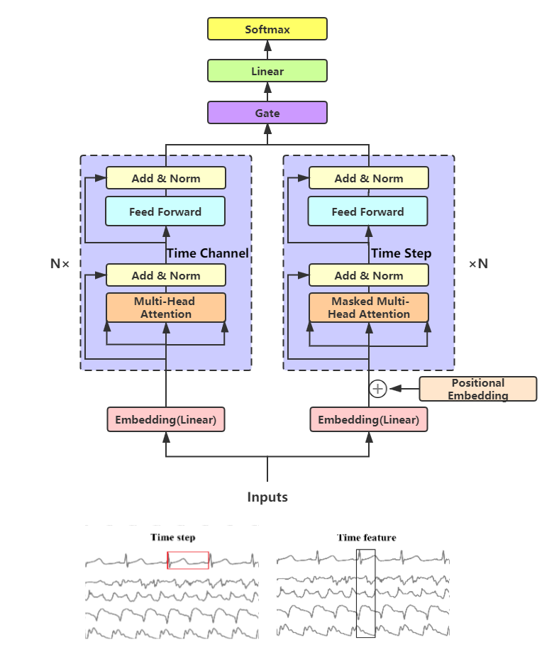
Figure 1: Model architecture of the Gated Transformer Networks.

Table 1: Test accuracy of GTN and other benchmark models on 13 multivariate time series dataset

	MLP	FCN	ResNet	Encoder	MCNN	t-LeNet	MCDCNN	Time-CNN	TWIESN	GTN
AUSLAN	93.3	97.5	97.4	93.8	1.1	1.1	85.4	72.6	72.4	97.5
ArabicDigits	96.9	99.4	99.6	98.1	10.0	10.0	95.9	95.8	85.3	98.8
CMUsubject1	60.0	100.0	99.7	98.3	53.1	51.0	51.4	97.6	89.3	100.0
CharacterTrajectories	96.9	99.0	99.0	97.1	5.4	6.7	93.8	96.0	92.0	97.0
ECG	74.8	87.2	86.7	87.2	67.0	67.0	50.0	84.1	73.7	91.0
JapaneseVowels	97.6	99.3	99.2	97.6	9.2	23.8	94.4	95.6	96.5	98.7
KickvsPunch	61.0	54.0	51.0	61.0	54.0	50.0	56.0	62.0	67.0	90.0
Libras	78.0	96.4	95.4	78.3	6.7	6.7	65.1	63.7	79.4	88.9
NetFlow	55.0	89.1	62.7	77.7	77.9	72.3	63.0	89.0	94.5	100.0
UWave	90.1	93.4	92.6	90.8	12.5	12.5	84.5	85.9	75.4	91.0
Wafer	89.4	98.2	98.9	98.6	89.4	89.4	65.8	94.8	94.9	99.1
WalkvsRun	70.0	100.0	100.0	100.0	75.0	60.0	45.0	100.0	94.4	100.0
PEMS	-	-	-	-	-	-	-	-	-	93.6

3.1 Embedding

In the original Transformers, the tokens are projected to a embedding layer. As time series data is continuous, we simply change the embedding layer to fully connected layer. Instead of linear projection, we add a non-linear activation $tanh$. Following Vaswani et al. (2017), the positional encoding is added with the non-linearly transformed time series data to encode the temporal information, as self-attention is hard to utilize the sequential correlation of time step.

3.2 Two-tower Transformer

Multivariate time series has multiple channels where each channel is a univariate time series. The common assumption is that there exists hidden correlation between different channels at current or warping time step. Capturing both the step-wise (temporal) and channel-wise (spatial) information is the key for multivariate time series research. One common approach is to exploit convolutions. That is, the reception field integrates both step-wise and channel-wise by the 2D kernels or the 1D kernels with fixed parameter sharing. Different from other works that leverage the original Transformer for time series classification and forecasting, we designed a simple extension of the two-tower framework, where the encoders in each tower explicitly capture the step-wise and channel-wise correlation by attention and masking, as shown in Figure 1.

Step-wise Encoder. To encode the temporal feature, we use the self-attention with mask to attend on each point cross all the channels by calculating the pair-wise attention weights among all the time steps. In the multi-head self-attention layers, the scaled dot-product attention formulates the attention matrix on all time step. Like the original Transformer architecture, position-wise fully connected feed-forward layers is stacked upon each multi-head attention layers for the enhanced feature extraction. The residual connection around each of the two sub-layers is also kept to direct information and gradient flow, following by the layer normalization.

Channel-wise Encoder. Likewise, the Channel-wise encoder calculates the attention weights among different channels across all the time step. Note that position of channel in the multivariate time series has no relative or absolute correlation, as if we switch the order of channels, the time series should has no changes. Therefore, we only add positional encoding in the Step-wise Encoder. Attention layers with the masking on all the channels is expected to explicitly capture the correlation among channels across all time step. Note that it is pretty straight-forward to implement both encoders by simply transpose the channel and time axis when feeding the time series for each encoders.

Table 2: Ablation study of the two-towers, gating and masking in GTN

	step-wise	step-wise+mask	channel-wise	channel-wise+mask	step-wise+channel-wise	GTN
					+concatenation
AUSLAN	97.0	95.3	94.5	94.5	96.7	97.5
ArabicDigits	98.6	98.5	98.3	98.3	98.9	98.8
CMUsubject16	96.0	96.6	100.0	100.0	96.3	100.0
CharacterTrajectories	96.0	97.1	96.9	96.5	97.5	97.0
ECG	87.0	84.0	92.0	89.0	86.0	91.0
JapaneseVowels	96.0	97.3	98.3	97.6	98.1	98.7
KickvsPunch	81.3	80.0	81.3	90.0	81.3	90.0
Libras	82.0	81.1	88.3	88.3	90.5	88.9
NetFlow	88.0	100.0	100.0	100.0	100.0	100.0
UWave	89.0	88.8	90.0	88.3	89.5	91.0
Wafer	97.0	98.1	96.9	97.9	97.9	99.1
WalkvsRun	96.4	100.0	96.5	100.0	100.0	100.0
PEMS	94.0	92.5	87.9	91.4	90.8	93.6

3.3 Gating

To merge the feature of the two towers which encodes step-wise and channel-wise correlations, a simple way is to concatenate all the features from two towers, which compromises the performance of both as shown in our ablation study.

Instead, we proposed a simple gating mechanism to learn the weight of each tower. After getting the output of each tower, which had a fully connect layer after each output of both encoders with non-linear activation as $C$ and $S$, we packed them into vector by concatenation followed by a linear projection layer to get $h$. After the softmax function, the gating weight are computed as $g_{1}$ and $g_{2}$. Then each gating weight is attending on the corresponding tower’s output and packed as the final feature vector.

$$h={\bf{W}}\cdot Concat(C,S)+b$$

$$g_{1},g_{2}=Softmax(h)$$

$$y=Concat(C\cdot g_{1},S\cdot g_{2})$$

(1)

4 Experiments

4.1 Experiment Settings

We test GTN on the same subset of the Baydogan archive Baydogan (2019), which contains 13 multivariate time series datasets. All the datasets have been split into training and testing by default, and there is no preprocessing for these time series. We choose the following deep learning models as the benchmarks.

• Fully Convolutional Networks (FCN) and Residual Networks (ResNet) Wang et al. (2017). These are reported to be among the best deep learning models in the multivariate time series classification task Ismail Fawaz et al. (2019). Multi-layer Perception (MLP) is also included as a simple baseline in our comparison.

• Universal Neural Network Encoder (Encoder) Serrà et al. (2018).

• Multi-scale Convolutional Neural Network (MCNN) Cui et al. (2016).

• Multi Channel Deep Convolutional Neural Network (MCDCNN) Zheng et al. (2016).

• Time Convolutional Neural Network (Time-CNN) Zhao et al. (2017).

• Time Le-Net (t-LeNet) Le Guennec et al. (2016).

• Time Warping Invariant Echo State Network (TWIESN) Tanisaro and Heidemann (2016).

The Gated Transformer Network is trained with Adagrad with learning rate 0.0001 and dropout = 0.2. The categorical cross-entropy is used as the loss function. Learning rate schedule on plateau Wang et al. (2017); Ismail Fawaz et al. (2019) is applied to train the GTN. We test on the training set and the test set every certain number of iterations, the best test results and its super parameters would be recorded. For fair comparison, we choose to report the test accuracy on the the model with the best training loss as Ismail Fawaz et al. (2019).

4.2 Results and Analysis

The results are shown in Table 1. GTN achieved comparable results with the FCN and ResNet. Note that the results has no statistical significant difference among these three models, though on NetFlow and KickvsPunch datasets, GTN shows superior performance. The drawback of GTN is comparably leaning to overfitting. Unlike FCN and ResNet where no dropout is used, the GTN has dropout binding with layer norm to reduce the risk of overfitting.

4.2.1 Ablation Study

To clearly state the performance gain from each module in the GTN, we performed a comprehensive study as shown in Table 2.

• Following the traditional Transformer, masking helps to ensure that the predictions for position $i$ can depend only on the known previous outputs and also helps the attention to not attend to the padding position. This benefits holds not only on the language but also on the time series data, as the tower-only transformer with mask are overall a bit better than the one without masks.

• Channel-wise only transformer outperforms step-wise only transformer on the majority of the dataset. This preliminary result supports our assumption that for multivariate time series, the correlation between different channels across all time step is an important differentiator with the univariate time series. The attention with mask is able to catch the channel-wise feature better.

• Different time series data might show different leaning on channel-wise and step-wise information. For example, on the dataset PEMS, the step-wise Transformer model works better. On the dataset CMUsubject16, the channel-wise Transformer model outperforms.

• Following the above point, exploiting both towers is a straight-forward solution. However, simple concatenation of the two towers sometimes works, but the performance always fall on the middle ground or even worse. Like on the dataset PEMS and CMUsubject16, step-wise model and channel-wise model works best for each cases. After concatenation of both towers’ feature, the results becomes even worse.

• By adding the gating weights before simple (equally-weighted) concatenation, the model is able to learn when to rely on a specific tower more by a pure data-driven way, thus show the best performance in this study.

4.3 Visualization and Analysis of the Attention Map

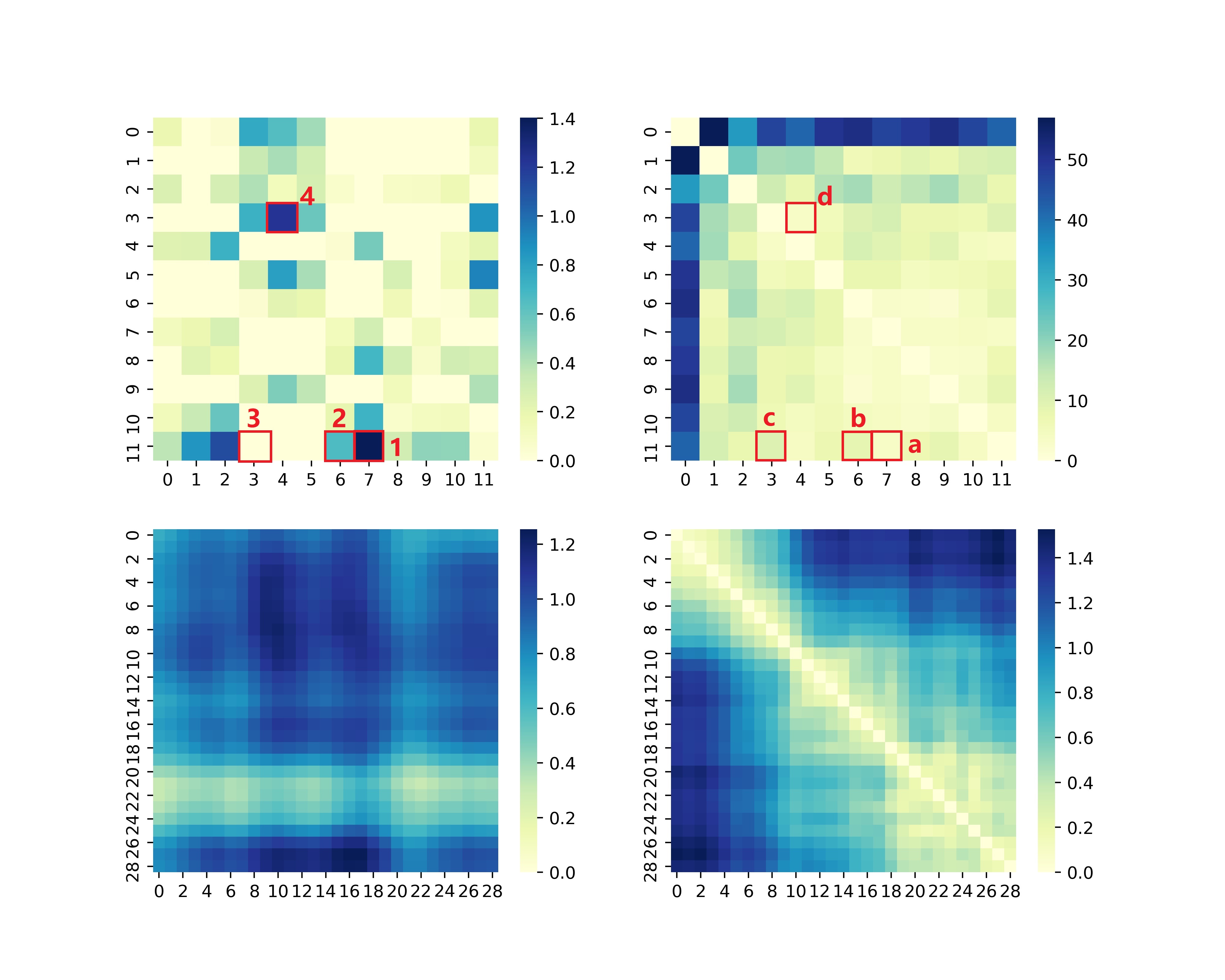
Figure 2: 1) channel-wise attention map (upper-left) 2) channel-wise DTW (upper-right) 3) step-wise attention map (bottom-left) 4) step-wise L2 distance (bottom-right)

The attention matrix represents the correlation between the channels and time steps respectively. We choose one sample from the JapaneseVowels dataset to visualize both attention maps. for the channel-wise attention map, we calculated the dynamic time warping (DTW) distance across the time series on different channel. For each time step, we also simply calculated the Euclidean distance across different channels, as on the same time step there is no time axis, thus DTW is not needed. The visualization is shown in Figure 2

Our first analysis focuses on the channel-wise attention map. In Fig 2, we label four blocks ($b1$-$b4$). In Fig 3, we draw the raw time series of the corresponding channels. We use $channel_{11}$ (abbreviated as $c11$, the same below) to represent channel 11 in the following analysis.

$b1$ and $b2$ have relatively high attention score, that is, both $c6$ and $c7$ are strongly co-fired with $c11$. Look at Fig 3, we can clearly see that $c6$ and $c7$ have relatively similar shapelet and trend with $c11$. Similarly, $b4$ have very high attention score, where $c3$ and $c4$ are also showing very similar trend. Meanwhile, $b3$ is among the one with very small attention score. Look at the $c11$ and $c3$, two time series show pretty much different even inverse trend. This preliminary finding is interesting because like the attention in NLP task where the attention score indicates the semantic correlation between different tokens, the channel-wise attention learned from the time series similarly shows the similar sequences that are co-fired together to force the learning lean to the final labels.

Note that the smaller DTW does not mean two sequence are similar. Like shown on the channel-wise DTW, block $c$ indicates very small DTW distance between $c3$ and $c11$. Actually $c11$ and $c3$ are very different in trends and shapelet. Our preliminary analysis shows that the channel-wise attention also tends to grab the similar sequences where DTW shows no clear differentiated factors.

As the step is fixed across channel for the step-wise attention, Euclidean distance is the special case of DTW at the same step, thus we choose Euclidean distance as the metric. Through the analysis of step-wise attention map and the Euclidean distance matrix, the distance between the time series and the similarity of the shapelet have an impact on who GTN calculates the attention scores, though the impact are not that obvious which deserves a deep dive in the future work.

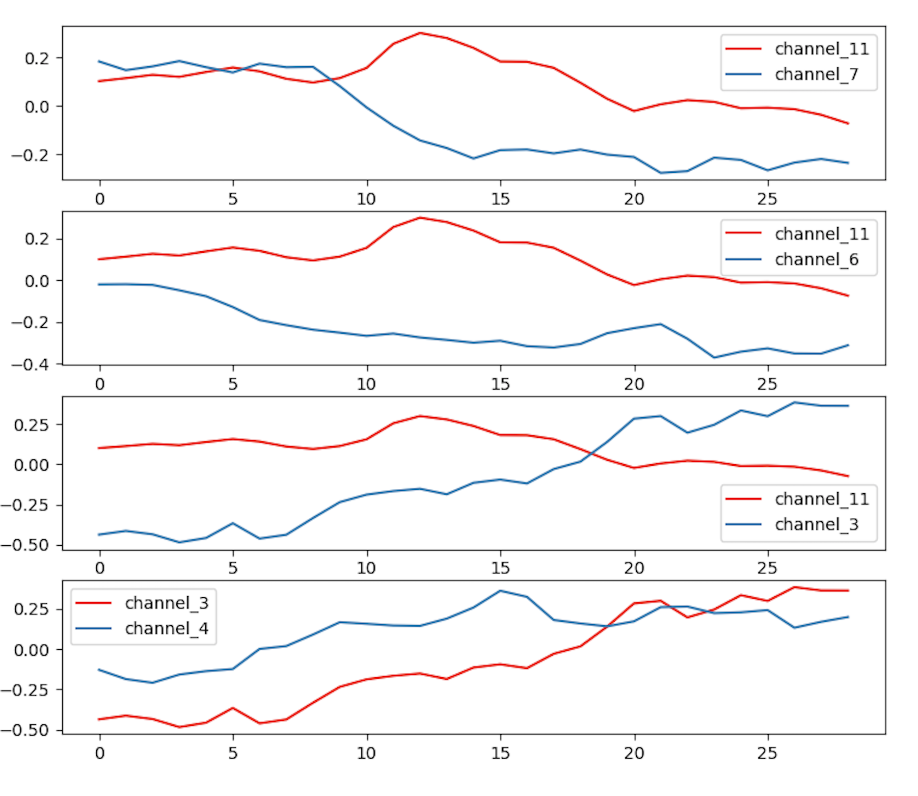
Figure 3: Drawing of the raw time series in different channel pairs.

4.4 Analysis on the Gating Weight

GTN has two towers to encode the step-wise and channel-wise information with self-attention respectively. With the gating method, the model learns to assign different weights to attend to these two Transformers. In the ablation study, we show that gating achieved better results compared with concatenation.

By observing the gate weights assigned to the two tower on the AULSAN data set, we found that for different sample, the gating weights assigned to step-wise and channel-wise tower are tends to be different, like $\{0.9899,0.0101\}$ and $\{0.0443,0.5557\}$ for two sample time series respectively. However, the gating weights overall show the trends to be skewed towards the step-wise tower, with the average gating weights of $\{0.7786,0.2214\}$. As shown in Table 2, the step-wise Transformer outperforms the channel-wise Transformer, thus overall the gating learns to assign more weights to the step-wise tower, the gating behavior and the results in the ablation study are consistent. The gating shows the capability to learn the weights from the data-driven manner to attend on each towers for different samples and dataset to improve the classification performance.

4.5 Analysis of the Embedding Output

As each time step are transformed to a dense vector through the embedding layer, we use the t-SNE Maaten and Hinton (2008) to reduce the dimension of the output from the embedding layer on AUSLAN. The result is shown in graph 4. The graph shows that all the points are clustered together on the specific manifold. We roughly labeled those clusters with five different colors.

As shown in Figure 5, we mapped each color back to the raw time series. Interestingly, the time step from each cluster are consistent and overall each cluster shows different shapelet.

• The green shapelet indicates a deep M shape.

• The light blue shapelet is a sharp trending-up sub-sequence.

• The dark blue shapelet is a plateau followed by a deep down like $7$.

• The magenta shapelet is like a recovering from the deep down with a bit trending up.

• The red shapelet is a plateau.

  By a closer look at the visualization of the embedding on each time step, the near points that forms some interesting shapelet has relatively smaller distance in the vector space. Like Liu and Wang (2016), where the author discover interesting shapelet by a well designed Markov transition matrix with the clustering on the transformed complex network graph, GTN shows the potential by learning the interesting pattern of some specific sub-sequences from scratch, which will be an interesting future work.

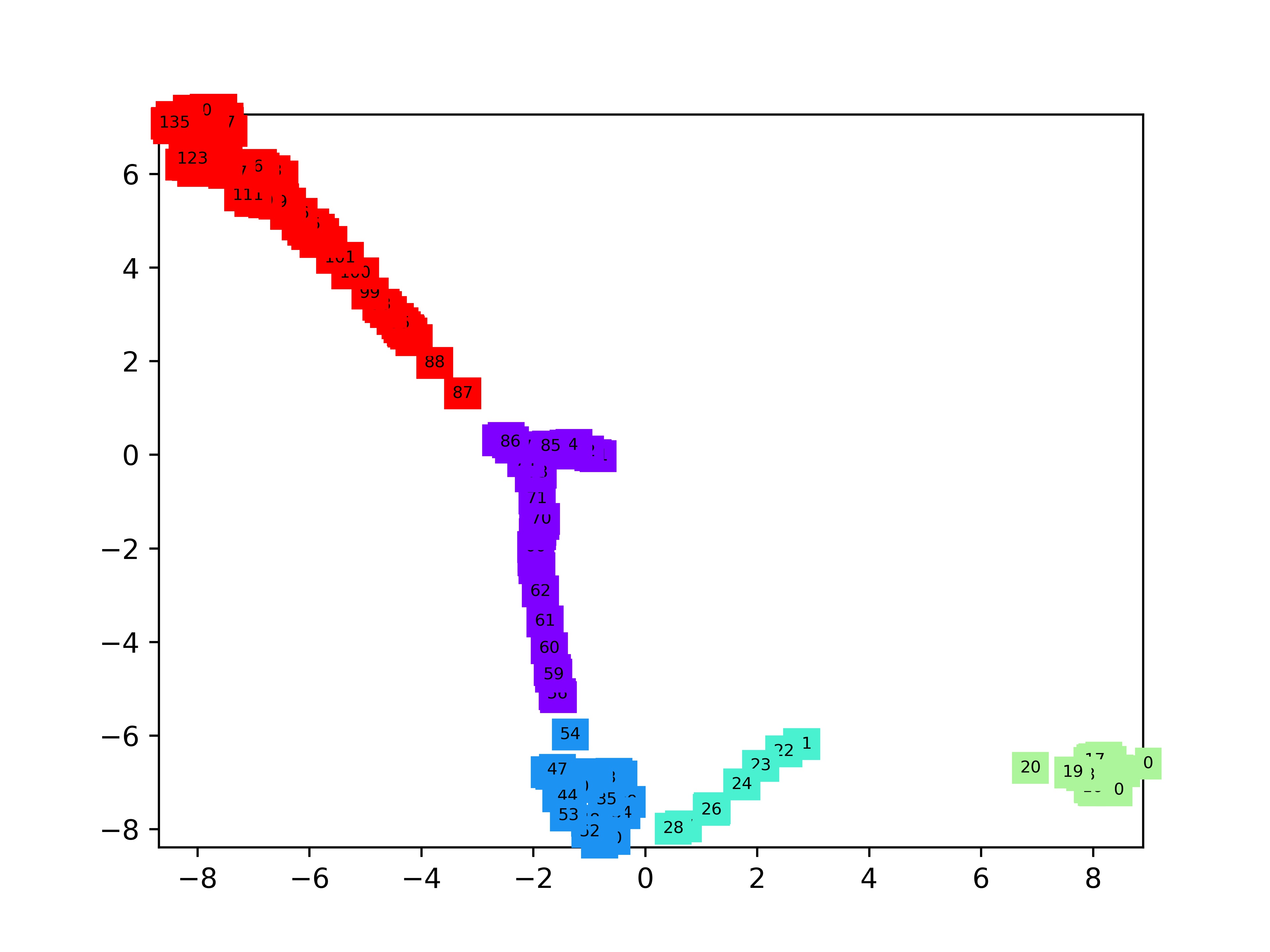
Figure 4: Visualization of the t-SNE result of the embedding layer output on the AUSLAN dataset.

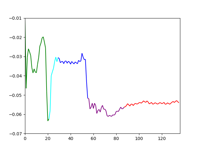
Figure 5: Shapelet discovered by the visualization of the embedding on each time step.

4.6 Visualization of the Extracted Feature

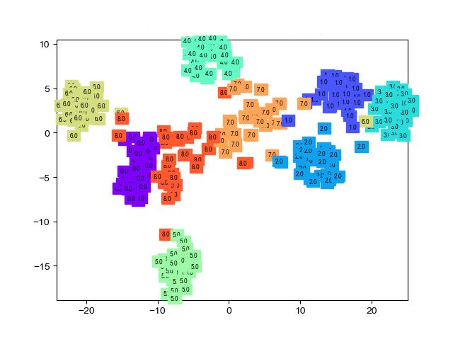
Figure 6: Visualization of the feature extracted after the gating in GTN.

lastly, following Ismail Fawaz et al. (2019), we visualize the feature vector after gating for a simple sanity check of the feature quality. We choose the JapaneseVowels dataset and apply t-SNE to reduce the dimension for visualization, as shown in Figure 6. Each number in the graph is the label with corresponding color encoding. and labels in the figure correspond to the labels of the original data. This figure shows that GTN is able to project the data into an easily separable space for better classification results.

5 Conclusion

We presented the Gated Transformer Network (GTN) as a simple extension of multidimensional time series using gating. With the gating that merges two towers of transformer networks which model the channel-wise and step-wise correlations respectively GTN is able to explicitly learn both channel-wise and step-wise correlations. We conducted comprehensive experiments on thirteen dataset and the preliminary results show that GTN is able to achieve competing performance with current state-of-the-art deep learning models. The ablation study shows how different modules work to together to achieve the improved performance. We also qualitatively analyzed the attention map and other components with visualization to better understand the interpretability of out model. Our preliminary results ground a solid foundation for the study of Transformer Network on the time series classification task in future research.

References

- Baydogan [2019] Mustafa Gokce Baydogan. Multivariate time series classification datasets, 2019.
- Cai et al. [2020] Ling Cai, Krzysztof Janowicz, Gengchen Mai, Bo Yan, and Rui Zhu. Traffic transformer: Capturing the continuity and periodicity of time series for traffic forecasting. Transactions in GIS, 24(3):736–755, 2020.
- Cui et al. [2016] Zhicheng Cui, Wenlin Chen, and Yixin Chen. Multi-scale convolutional neural networks for time series classification. arXiv preprint arXiv:1603.06995, 2016.
- Devlin et al. [2018] Jacob Devlin, Ming-Wei Chang, Kenton Lee, and Kristina Toutanova. Bert: Pre-training of deep bidirectional transformers for language understanding. arXiv preprint arXiv:1810.04805, 2018.
- Ismail Fawaz et al. [2019] Hassan Ismail Fawaz, Germain Forestier, Jonathan Weber, Lhassane Idoumghar, and Pierre-Alain Muller. Deep learning for time series classification: a review. Data Mining and Knowledge Discovery, 33(4):917–963, 2019.
- Karim et al. [2017] Fazle Karim, Somshubra Majumdar, Houshang Darabi, and Shun Chen. LSTM fully convolutional networks for time series classification. CoRR, abs/1709.05206, 2017.
- Keogh [2002] Eamonn Keogh. Exact indexing of dynamic time warping - sciencedirect. VLDB ’02: Proceedings of the 28th International Conference on Very Large Databases, pages 406–417, 2002.
- Le Guennec et al. [2016] Arthur Le Guennec, Simon Malinowski, and Romain Tavenard. Data augmentation for time series classification using convolutional neural networks. 2016.
- Li et al. [2019] Shiyang Li, Xiaoyong Jin, Yao Xuan, Xiyou Zhou, Wenhu Chen, Yu-Xiang Wang, and Xifeng Yan. Enhancing the locality and breaking the memory bottleneck of transformer on time series forecasting. In Advances in Neural Information Processing Systems, pages 5243–5253, 2019.
- Liu and Wang [2016] Lu Liu and Zhiguang Wang. Encoding temporal markov dynamics in graph for visualizing and mining time series. arXiv preprint arXiv:1610.07273, 2016.
- Maaten and Hinton [2008] Laurens van der Maaten and Geoffrey Hinton. Visualizing data using t-sne. Journal of machine learning research, 9(Nov):2579–2605, 2008.
- Oh et al. [2018] Jeeheh Oh, Jiaxuan Wang, and Jenna Wiens. Learning to exploit invariances in clinical time-series data using sequence transformer networks. arXiv preprint arXiv:1808.06725, 2018.
- Rußwurm and Körner [2020] Marc Rußwurm and Marco Körner. Self-attention for raw optical satellite time series classification. ISPRS Journal of Photogrammetry and Remote Sensing, 169:421 – 435, 2020.
- Serrà et al. [2018] Joan Serrà, Santiago Pascual, and Alexandros Karatzoglou. Towards a universal neural network encoder for time series. In CCIA, pages 120–129, 2018.
- Tanisaro and Heidemann [2016] Pattreeya Tanisaro and Gunther Heidemann. Time series classification using time warping invariant echo state networks. In 2016 15th IEEE International Conference on Machine Learning and Applications (ICMLA), pages 831–836. IEEE, 2016.
- Vaswani et al. [2017] Ashish Vaswani, Noam Shazeer, Niki Parmar, Jakob Uszkoreit, Llion Jones, Aidan N Gomez, Łukasz Kaiser, and Illia Polosukhin. Attention is all you need. In Advances in neural information processing systems, pages 5998–6008, 2017.
- Wang et al. [2017] Z. Wang, W. Yan, and T. Oates. Time series classification from scratch with deep neural networks: A strong baseline. In 2017 International Joint Conference on Neural Networks (IJCNN), pages 1578–1585, 2017.
- Yang et al. [2015] Jianbo Yang, Minh Nhut Nguyen, Phyo Phyo San, Xiaoli Li, and Shonali Krishnaswamy. Deep convolutional neural networks on multichannel time series for human activity recognition. In Ijcai, volume 15, pages 3995–4001. Buenos Aires, Argentina, 2015.
- Zhao et al. [2017] Bendong Zhao, Huanzhang Lu, Shangfeng Chen, Junliang Liu, and Dongya Wu. Convolutional neural networks for time series classification. Journal of Systems Engineering and Electronics, 28(1):162–169, 2017.
- Zheng et al. [2016] Yi Zheng, Qi Liu, Enhong Chen, Yong Ge, and J Leon Zhao. Exploiting multi-channels deep convolutional neural networks for multivariate time series classification. Frontiers of Computer Science, 10(1):96–112, 2016.