Synthesizing Linked Data Under
ardinality and Integrity Constraints

Abstract.

The generation of synthetic data is useful in multiple aspects, from testing applications to benchmarking to privacy preservation. Generating the links between relations, subject to cardinality constraints (CCs) and integrity constraints (ICs) is an important aspect of this problem. Given instances of two relations, where one has a foreign key dependence on the other and is missing its foreign key ($FK$) values, and two types of constraints: (1) CCs that apply to the join view and (2) ICs that apply to the table with missing $FK$ values, our goal is to impute the missing $FK$ values such that the constraints are satisfied. We provide a novel framework for the problem based on declarative CCs and ICs. We further show that the problem is NP-hard and propose a novel two-phase solution that guarantees the satisfaction of the ICs. Phase i@ yields an intermediate solution accounting for the CCs alone, and relies on a hybrid approach based on CC types. For one type, the problem is modeled as an Integer Linear Program. For the others, we describe an efficient and accurate solution. We then combine the two solutions. Phase ii@ augments this solution by incorporating the ICs and uses a coloring of the conflict hypergraph to infer the values of the $FK$ column. Our extensive experimental study shows that our solution scales well when the data and number of constraints increases. We further show that our solution maintains low error rates for the CCs.

1. Introduction

In recent years, we have witnessed an increase in data-centric applications that call for efficient testing over reliable databases with certain desired qualities (BrunoC05; LoCH10). Existing benchmarks such as TPC-H (tpchPaper; tpch) may not possess the desired characteristics for testing a specific application as they may not have the needed statistical qualities or the correct Integrity Constraints (ICs). The field of data generation (MannilaR89; GraySEBW94; HoukjaerTW06; BinnigKLO07; Arasu2011; RablDFSJ15; FazekasK18; SanghiSHT18) has proven effective in this respect. Two prominent challenges in this field are: (1) the generation of links between different tables, i.e., aligning foreign keys with primary keys based on Cardinality Constraints (CCs) (Arasu2011), and (2) ensuring that the data will satisfy a set of expected ICs (SoltanaSB17).

In particular, when the real data is sensitive and access to it is heavily regulated, users often need to wait months or years to get access to the real data before they can even start writing data analysis programs. One solution is to generate realistic synthetic data that satisfies some CCs and ICs so that users can: (a) start writing code to analyse the data, (b) test it locally, and (c) evaluate whether access to the data would be useful for their purposes even before they get access to the real data. However, current methods for generating synthetic data under privacy constraints (especially state-of-the-art standards like differential privacy (Dwork06)) do not handle data with a combination of CCs or statistical constraints and ICs. Most, (e.g., (ZhangCPSX17; HeMD14; SnokeS18)), only handle statistical constraints.

Furthermore, there has been a lot of recent work on answering count queries under differential privacy (e.g., Matrix mechanism (LiMHMR15), HDMM (McKennaMHM18)) and in particular over relational databases (KotsogiannisTHF19). A key challenge when answering queries especially over relational databases is that of consistency – are the answers outputted by a differentially private algorithm consistent with some underlying database? While there is work on using inference to enforce consistency when all the count queries are over a single view of the underlying database (HayRMS10), these techniques do not extend to the case when: (a) the underlying database is relational and query answers are over several joined views of the relations, and (b) when the underlying database needs to satisfy some ICs. One solution to this problem is to find a database that is consistent with the query answers and the ICs, and answer queries from it. While techniques for finding such a consistent database are known for single tables without ICs (HayRMS10; LiHMW14; BarakCDKMT07), no such techniques are known when there are multiple tables in a relational database with ICs.

Moreover, DBMS testing and other applications may require databases that conform to both CCs and ICs to make them more realistic (Arasu2011; SoltanaSB17). For instance, consider a table with the attributes $A$ and $B$. A query grouping over attributes $A$ and $B$ could return as many tuples as the cross product of the active domains of $A$ and $B$. However, if there is a Functional Dependency $A\rightarrow B$, then the output size of the group-by query is only the maximum of the active domains of the two attributes. Thus, the presence of ICs can significantly impact the performance characteristics of queries.

Persons (rel. $R_{1}$)

$p_{id}$	$Age$	$Rel$	$Multi$-$ling$	$h_{id}$
$1$	$75$	$Owner$	$0$	?
$2$	$75$	$Owner$	$1$	?
$3$	$25$	$Owner$	$0$	?
$4$	$25$	$Owner$	$1$	?
$5$	$24$	$Spouse$	$0$	?
$6$	$10$	$Child$	$1$	?
$7$	$10$	$Child$	$1$	?
$8$	$30$	$Owner$	$0$	?
$9$	$30$	$Owner$	$1$	?

Housing (rel. $R_{2}$)

$h_{id}$	$Area$
$1$	$Chicago$
$2$	$Chicago$
$3$	$Chicago$
$4$	$Chicago$
$5$	$NYC$
$6$	$NYC$

Figure 1. Database $\mathcal{D}$ with FK $h_{id}$ missing from $R_{1}$

⬇

$DC_{O,O}:$ $\forall t_{1},t_{2}.~{}\neg(t_{1}.Rel=t_{2}.Rel=Owner\land t_{1}.h_{id}=t_{2}.h_{id})$

$DC_{O,S,low}:$ $\forall t_{1},t_{2}.~{}\neg(t_{1}.Rel=Owner\land t_{2}.Rel=Spouse\land$

$t_{2}.Age<t_{1}.Age-50\land t_{1}.h_{id}=t_{2}.h_{id})$

$DC_{O,S,up}:$ $\forall t_{1},t_{2}.~{}\neg(t_{1}.Rel=Owner\land t_{2}.Rel=Spouse\land$

$t_{2}.Age>t_{1}.Age+50\land t_{1}.h_{id}=t_{2}.h_{id})$

$DC_{O,C,low}:$ $\forall t_{1},t_{2}.~{}\neg(t_{1}.Rel=Owner\land t_{1}.\leavevmode\color[rgb]{0,0,0}{Multi\text{-}ling=1}\land t_{2}.Rel=$

$Child\land t_{2}.Age<t_{1}.Age-50\land t_{1}.h_{id}=t_{2}.h_{id})$

$DC_{O,C,up}:$ $\forall t_{1},t_{2}.~{}\neg(t_{1}.Rel=Owner\land t_{1}.\leavevmode\color[rgb]{0,0,0}{Multi\text{-}ling=1}\land t_{2}.Rel=$

$Child\land t_{2}.Age>t_{1}.Age-12\land t_{1}.h_{id}=t_{2}.h_{id})$

(a) Denial Constraints: $DC_{O,O}$ enforces that no two homeowners can reside in the same home, $DC_{O,S,low}$ and $DC_{O,S,up}$ together specify the permissible age range of a spouse in any home, and $DC_{O,C,low}$ and $DC_{O,C,up}$ give the age range for a child living with a multi-lingual homeowner

⬇

$CC_{1}:$ $|\sigma_{Rel=Owner,Area=Chicago}(R_{1}\bowtie R_{2})|=4$

$CC_{2}:$ $|\sigma_{Rel=Owner,Area=NYC}(R_{1}\bowtie R_{2})|=2$

$CC_{3}:$ $|\sigma_{Age\leq 24,Area=Chicago}(R_{1}\bowtie R_{2})|=3$

$CC_{4}:$ $|\sigma_{\leavevmode\color[rgb]{0,0,0}{Multi\text{-}ling=1},Area=Chicago}(R_{1}\bowtie R_{2})|=4$

(b) Cardinality Constraints: $CC_{1}$ and $CC_{2}$ give the number of homeowners in Chicago and NYC, resp., $CC_{3}$ gives the number of people younger than $25$ who live in Chicago, and $CC_{4}$ gives the number of multi-lingual individuals in Chicago.

Figure 2. Set of DCs and set of CCs

In this paper, we investigate the problem of generating the links between database tables based on a set of linear CCs and a set of ICs.

Formally, we consider two relations, $R_{1}$ and $R_{2}$, where $R_{1}$ has a foreign key dependence on $R_{2}$ and is missing all values in its foreign key column $FK$. The goal is to impute $FK$ in $R_{1}$ based on the given CCs and ICs. Importantly, this problem and our solutions can be extended to relational databases with a snowflake schema (10.1145/248603.248616), by focusing on pairs of relations linked by foreign key joins.

Example 1.1.

Consider the relations in Figure 1 based on the Census database. $R_{1}$ describes people through attributes such as age, relationship to a household (e.g. owner or spouse), whether they speak more than $1$ language and a (missing) household id, whereas $R_{2}$ shows the area for each household. In addition, we are given the set of ICs and CCs in Figures 2(a) and 2(b), respectively. The goal is to impute values in the $h_{id}$ column in $R_{1}$ so that the ICs and CCs are satisfied.

We believe that the problem we focus on is a key building block for the general problem of synthesizing data consistent with CCs and ICs for all three use-cases mentioned above. In particular, we believe that one can use the wealth of existing literature to synthesize individual relations consistent with CCs without the key relationships and then use our technique to fill-in the foreign keys.

Our Contributions

We model the problem, give a theoretical analysis, and provide a solution for the generation of foreign keys for existing database relations while ensuring the satisfaction of a set of ICs and reducing the error of a set of CCs. Next, we give our main contributions.

Model and Theoretical Results: We define the problem of C-Extension whose input is a relation $R_{1}$ with an unknown foreign key dependence on a relation $R_{2}$, i.e., the $FK$ column in $R_{1}$ is missing, and a set of CCs and ICs. For the CCs, we define and use linear CCs that apply to $R_{1}\bowtie R_{2}$, based on (Arasu2011). For the ICs, we define a type of Denial Constraints (DCs) (ChomickiM05; ChuIP13), called Foreign Key DCs, that applies to $R_{1}$ and forbids tuples from having the same $FK$ value under specified conditions. We then show that C-Extension is NP-hard in data complexity. This result leads us to a two-phase heuristic solution that still ensures the satisfaction of all DCs, while tolerating possible errors in the CC counts.

Solution: Our solution can be split into two phases: (1) first phase (Section 4) is designed for the completion of a view $V_{Join}$ based on CCs, where $V_{Join}$ represents $R_{1}\bowtie R_{2}$ and is initialized with a copy of $R_{1}$ (without the $FK$ column) along with an empty column per non-key column in $R_{2}$ (due to foreign key dependence, $|R_{1}|=|V_{Join}|$), and (2) second phase (Section 5) uses the generated view $V_{Join}$ to complete the $FK$ column in $R_{1}$ so that the DCs are satisfied.

Phase i@: We provide a novel description of CC relationships that allows for $V_{Join}$ to be completed efficiently and precisely under specific conditions (presented in Section 3.1). We further devise algorithms for this case and the general case:

• For the general case, we devise an algorithm that models the CCs and the tuples in $V_{Join}$ as an Integer Linear Program (inspired by (Arasu2011)). From its solution, we greedily infer the values in $V_{Join}$ for the attributes that come from $R_{2}$.

• For the special case, we devise a novel algorithm based on relationships between the CCs. We show that if the CCs have containment or disjointness relationships between them (defined in Section 4.2), then we can find an exact completion of $V_{Join}$ without any errors, provided one exists.

Our approach is a hybrid of these two solutions that employs the first solution for the subset of CCs that does not fit the special case, and employs the second solution for the subset of CCs that does.

Another novelty in our solution exploits the fact that the all-way marginals for $R_{1}$, i.e., counts of tuples with different combinations of values in $R_{1}$’s non-key columns, have the same counts in $V_{Join}$. Thus, we augment the input set of CCs to improve accuracy.

Phase ii@: For the second phase, we employ the concept of a conflict hypergraph (ChuIP13) and use a novel algorithm based on hypergraph coloring. We model the tuples in $R_{1}$ as vertices and connect by an edge every set of tuples that will violate a DC if assigned the same foreign key. Thus, colors represent the values that the foreign keys can take in $R_{1}$, and a proper coloring represents a mapping of tuples to foreign keys that does not violate any DC. Due to the previous stage that considered $R_{1}\bowtie R_{2}$, tuples in $R_{1}$ have a certain list of permitted colors. This version of the graph coloring problem is called List Coloring (achlioptas_molloy_1997) and is known to be NP-hard. To color the graph, we use a greedy coloring algorithm that considers vertices in descending order by degrees. The algorithm skips vertices whose list of permitted colors is subsumed by the colors assigned to their neighbors. We ensure a proper coloring by adding the least number of new colors for the skipped vertices. Adding colors beyond the permitted lists corresponds to artificially adding tuples in $R_{2}$.

Experimental Evaluation We have implemented our solution and performed a comprehensive set of experiments on a dataset derived from the 2010 U.S. Decennial Census (sexton_abowd_schmutte_vilhuber_2017). We have evaluated our solution in terms of accuracy and scalability in various scenarios, several of which were used for comparison with a baseline based on (Arasu2011). We further examined the runtime breakdown of our approach, presenting the runtimes of phases i@ and ii@ in our solution. Our results indicate that our solution incurs relatively small error for CCs and no error for DCs (as guaranteed by our theoretical analysis). Moreover, our algorithms scale well for large data sizes, and large and complex sets of CCs and DCs. For increasing data scales, our approach was $17$ times faster on average across different cases than the baseline we compare to.

2. Preliminaries and Model

We now define the basic concepts used throughout the paper, and the C-Extension problem.

Relations in a Database: Let $R_{1}$ and $R_{2}$ be relations over the schema attributes $(K_{1},A_{1},\ldots,A_{p},$ $FK)$ and $(K_{2},B_{1},\ldots,B_{q})$, respectively. An attribute $A_{j}$ of $R_{i}$ may also be called a column and is denoted by $R_{i}.A_{j}$. $t\in R_{i}$ denotes a tuple in $R_{i}$ and $t.A_{j}$ denotes the cell of column $A_{j}$ in tuple $t$. The last column in $R_{1}$ ($FK$) is a foreign key column that gets its values from the key column $K_{2}$ in $R_{2}$. The view $V_{Join}=R_{1}\bowtie_{FK=K_{2}}R_{2}$ denotes the join of the two relations. If all values of a column $A_{i}$ are missing, it is called a missing column.

Example 2.1.

Consider a database $\mathcal{D}$ with two relations $R_{1}$ and $R_{2}$ as shown in Figure 1. $R_{1}.h_{id}$ is a missing column. The first row in $R_{1}$ says that $t_{1}.Age$ is $75$, $t_{1}.Rel$ is Owner and $t_{1}.Multi$-$ling$ is $0$.

Foreign Key Denial Constraints: DCs (ChomickiM05) are a general form of constraints that can be written as a negated First Order Logic statement. DCs can express several types of integrity constraints like functional dependencies and conditional functional dependencies (bohannon2007conditional). In this paper, we restrict our attention to DCs that contain a condition of the form $t_{1}.FK=\ldots=t_{k}.FK$.

Definition 2.2 (Foreign Key DC).

A Foreign Key DC on a relation $R(K_{1},A_{1},\ldots,$ $A_{p},FK)$ is defined as the following FOL statement:

⬇

$\forall t_{1},t_{2},\ldots,t_{k}.~{}$ $\neg(p_{1}\land\ldots\land p_{n})$

where $p_{q}=t_{i}.A_{l}\circ t_{j}.A_{l}$ or $p_{q}=t_{i}.A_{l}\circ c$, for $t_{i},t_{j}\in R$, $p\geq 2$, $\circ\in\{=,<,>,\neq\}$, $c$ and $k$ are constants, and $p_{n}=(t_{1}.FK=\ldots=t_{k}.FK)$.

We use the terms Foreign Key DC and DC interchangeably.

Example 2.3.

$DC_{O,O}$ (Figure 2(a)), which states that two homeowners cannot be in the same home, can be formulated as follows:

⬇

$\forall t_{1},t_{2}\in R_{1}.~{}\neg(t_{1}.Rel=t_{2}.Rel=Owner\land t_{1}.h_{id}=t_{2}.h_{id})$

Note that the restriction to Foreign Key DCs means that all constraints are on people that are in the same household.

Linear Cardinality Constraints: CCs form the second class of constraints that allows for the specification of the number of tuples that should posses a certain set of attribute values, which can be expressed as a selection condition. As standard in previous work (Arasu2011; Mckenna2019), we restrict our attention to linear CCs.

Definition 2.4 (Linear CC, adapted from (Arasu2011)).

A linear CC over a database $\mathcal{D}$ consisting of relations $R_{1}(K_{1},A_{1},\ldots,A_{p},FK)$ and $R_{2}(K_{2},B_{1},\ldots,$ $B_{q})$ is defined as follows:

⬇

$|\sigma_{\varphi}(R_{1}\bowtie_{FK=K_{2}}R_{2})|=k$

where $\varphi$ is a Boolean selection predicate over a subset of (non-key) attributes in $\mathcal{D}$, and $k\in\mathbb{N}$.

In the rest of the paper, we only refer to conjunctive selection predicates with conjuncts of the form $A_{i}\circ c$, where $\circ\in\{=,<,>,\leq,\geq\}$ and $c$ is in the domain of column $A_{i}$, though our algorithms can be extended to conditions that contain disjunction as well.

Example 2.5.

$CC_{1}$ (Figure 2(b)), which states that the number of homeowners ($Rel=$ Owner) living in $Area=Chicago$ must equal $4$, can be written as: $|\sigma_{Rel=Owner,Area=Chicago}~{}R_{1}\bowtie R_{2}|=4$.

We denote by $R\vDash\sigma$ the fact that relation $R$ meets constraint $\sigma$.

Problem Definition: We now formally define the C-Extension problem and discuss its intractability.

Definition 2.6 (C-Extension).

Let $R_{1}(K_{1},A_{1},\dots,A_{p},FK)$ and $R_{2}(K_{2},$ $B_{1},\dots,B_{q})$ be two relations, where $R_{1}.FK$ is a foreign key mapped from $R_{2}.K_{2}$ and is empty . Let $S_{DC}$ denote the set of DCs over $R_{1}$ and let $S_{CC}$ denote the set of linear CCs over the foreign key join between $R_{1}$ and $R_{2}$. C-Extension is the problem of completing all the values in $R_{1}.FK$ to create $\hat{R_{1}}$ so that (1) $\forall\sigma\in S_{DC},~{}\hat{R_{1}}\vDash\sigma$, (2) $\forall\sigma\in S_{CC},~{}\hat{R_{1}}\bowtie_{FK=K_{2}}R_{2}\vDash\sigma$.

Example 2.7.

Reconsider relations $R_{1}$ and $R_{2}$ in Figure 1, and DCs and CCs in Figure 2. A solution $\hat{R_{1}}$ for the C-Extension problem as defined by these relations and constraints is shown in Figure 3.

Persons (rel. $R_{1}$)

$p_{id}$	$Age$	$Rel$	$Multi$-$ling$	$h_{id}$
$1$	$75$	$Owner$	$0$	$2$
$2$	$75$	$Owner$	$1$	$1$
$3$	$25$	$Owner$	$0$	$3$
$4$	$25$	$Owner$	$1$	$4$
$5$	$24$	$Spouse$	$0$	$2$
$6$	$10$	$Child$	$1$	$2$
$7$	$10$	$Child$	$1$	$2$
$8$	$30$	$Owner$	$0$	$5$
$9$	$30$	$Owner$	$1$	$6$

Figure 3. Relation $R_{1}$ from Figure 1 with FK $h_{id}$ filled-in to satisfy DCs and CCs given in Figure 2

The decision version of C-Extension is given by the same setting as in Definition 2.6. The output is $1$ if there exists a completion of $R_{1}.FK$ such that all DCs and CCs are satisfied, and $0$ otherwise.

Proposition 2.8.

The decision problem version of C-Extension is NP-hard in data complexity.

Proof Sketch.

We describe a reduction from NAE-3SAT to C-Extension. In the NAE-3SAT problem, we are given a 3-CNF formula $\varphi$ and asked whether there is a satisfying assignment to $\varphi$ with every clause having at least one literal with the value False. Given a 3-CNF formula $\varphi=C_{1}\land\ldots\land C_{n}$, where $x_{1},\ldots,x_{m}$ are the propositional variables in $\varphi$, construct a relation $R_{1}(Var,\alpha,Cls,Chosen)$, where $Chosen$ is missing all values, and $Var,\alpha,Cls$ columns take values:

1. $(x_{i},1,C_{j},?)$ if making $x_{i}$ True makes $C_{j}$ True

2. $(x_{i},0,C_{j},?)$ if making $x_{i}$ False makes $C_{j}$ True

We define $S_{DC}$ to be the set with the following two DCs:

1. $\forall t_{1},t_{2}.~{}\neg(t_{1}.Var$=$t_{2}.Var\land t_{1}.\alpha\neq t_{2}.\alpha\land t_{1}.Chosen$=$t_{2}.Chosen)$

2. $\forall t_{1},t_{2},t_{3}.~{}\neg(t_{1}.Cls$=$t_{2}.Cls$=$t_{3}.Cls\land t_{1}.Chosen$=$t_{2}.Chosen$= $t_{3}.Chosen)$

CCs are not needed in the reduction. The goal is to complete the missing column $Chosen$ in $R_{1}$. We define $R_{2}$ as containing two columns: a primary key column $Chosen$, and another column $E$. $R_{2}$ contains the tuples $(0,a)$ and $(1,b)$, i.e., the domain for $Chosen$ is $\{0,1\}$. Intuitively, $Chosen$ encodes the satisfying assignment for $\varphi$ by assigning values to each tuple, where $t.Chosen$=$1$ iff the assignment should be $t.Var$=$t.\alpha$. ∎

The full proofs are detailed in Section LABEL:sec:proofs of the appendix.

3. Solution Overview

Our solution proceeds in two phases as seen in Figure 4. In phase i@, we consider the view $V_{Join}$ representing the join of the two relations $R_{1}$ and $R_{2}$, where $R_{1}$ has a foreign key dependence on $R_{2}$, and initialize it with (non $FK$) columns from $R_{1}$ and an empty column per non-key column from $R_{2}$. We infer these values based on the CCs by a hybrid approach that uses both ILP (Arasu2011) and a more efficient and accurate procedure for special cases. In phase ii@, we impute $R_{1}.FK$ by modeling the problem as a conflict hypergraph using the DCs, and coloring it based on the inferred values in $V_{Join}$.

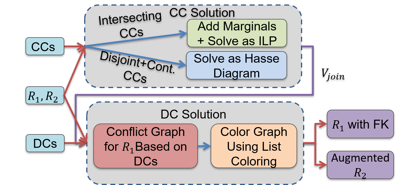
Figure 4. Solution Overview

3.1. Overview of the First Phase

Due to the foreign key dependence (Definition 2.6), we define $V_{Join}$ over the columns $K_{1},A_{1},\ldots,A_{p},B_{1},\ldots,B_{q}$ such that $t\in R_{1}$ implies that there is a single $t^{\prime}\in V_{Join}$ with $t.K_{1}$=$t^{\prime}.K_{1}$ and $\forall 1\leq i\leq p.~{}t.A_{i}=t^{\prime}.A_{i}$ with additional $B_{1},\ldots,B_{q}$ entries that are initially all empty because $FK$ is missing in $R_{1}$. Therefore, $|V_{Join}|=|R_{1}|$. Our goal is to complete these columns based on the CCs.

Example 3.1.

Reconsider $R_{1}$ and $R_{2}$ shown in Figure 1 and the CCs in Figure 2(b). The join view $V_{Join}$ is $R_{1}$ as it appears in Figure 1 (without $h_{id}$) with an empty Area column (as this is the schema of $R_{1}\bowtie R_{2}$). Due to the foreign key dependency, we have $|V_{Join}|=|R_{1}|$, and $V_{Join}$ contains a tuple for each $R_{1}$ tuple with the same values as in $R_{1}$ and an empty $Area$ value. The reason is that the $FK$ values are missing in $R_{1}$. Our goal is to fill-in $V_{Join}$ so that the CCs are satisfied.

We give a short description of our solution for completing $V_{Join}$.

Solution as an ILP (Section 4.1, green box in Figure 4): Given a set of CCs on $V_{Join}$, we model the problem of completing the missing columns as a system of linear equations with variables accounting for counts of different tuples needed in $V_{Join}$ to satisfy the CCs. Thus, the variables must take non-negative integer values. We artificially add to $S_{CC}$ all-way marginals (using the idea of intervalization from (Arasu2011) that is explained in Section 4) from $R_{1}$ to enhance the accuracy of the solution. For example, based on CCs given in Example 1.1, $|\sigma_{Age\leq 24,Rel=Spouse,Multi\text{-}ling=0}|=1$ gets added to $S_{CC}$. We then assign $B_{1},\ldots,B_{q}$ values to the tuples in $V_{Join}$ based on the solution returned by an ILP solver.

Using CC Relationships for Special Cases (Section 4.2, blue box in Figure 4): We give a novel description of the relationships between CCs based on their selection conditions, defining CC containment, disjointness and intersection. In the case where there are no intersecting CCs and no disjunctions, we give an algorithm to complete $V_{Join}$ that models the containment and disjointness of CCs as a Hasse diagram (williamson2002combinatorics) that it recurses on bottom-up to fill-in $V_{Join}$. Any leftover $V_{Join}$ tuples without $B_{1},\ldots,B_{q}$ values are randomly assigned a combination that cannot cause a new contribution towards the target count of any CC. However, if no such combinations are available, then the leftover $V_{Join}$ tuples cannot be completed. We refer to these as invalid tuples.

Hybrid Approach (Section 4.3): In the absence of intersecting CCs, the solution decomposes cleanly as seen above. This motivates the hybrid approach that combines ideas from both cases to achieve better runtime and accuracy when some CCs intersect. We start by labeling each pair of CCs as disjoint, contained or intersecting. For all CCs that do not intersect or contain any intersecting CCs, we use the approach from Section 4.2, and for the rest, we use the ILP approach from Section 4.1. Lastly, as seen above in the special case, we may end up with some invalid tuples.

3.2. Overview of the Second Phase

After filling-in the columns of $V_{Join}$ that originate in $R_{2}$ ($B_{1}\ldots,B_{q}$), we turn to reverse-engineering $R_{1}$ from $V_{Join}$. This phase uses conflict hypergraphs (ChuIP13) to represent possible DC violations.

Conflict Hypergraph (Section LABEL:subsec:list_coloring, red box in Figure 4): We use the notion of conflict hypergraph for the tuples of $R_{1}$ based on the DCs. Given a DC, we construct an edge for all the sets of tuples that cannot get the same foreign key value due to that DC.

Example 3.2.

Consider the relation $R_{1}$ depicted in Figure 1 and the first DC in Figure 2(a). Suppose the first two tuples are assigned the same $Area$ value in $V_{Join}$. Thus, the conflict hypergraph will have an edge containing the tuples with $p_{id}=1$ and $p_{id}=2$ since they are both owners and cannot be in the same household (the $h_{id}$ value). The conflict hypergraph of our running example is depicted in Figure LABEL:fig:graph.

List Coloring (Section LABEL:subsec:list_coloring, orange box in Figure 4): Proper coloring of the hypergraph ensures that there must be at least two vertices in each edge with distinct colors. Thus, modeling each $FK$ value as a color and each tuple as a vertex allows us to prove that a proper coloring results in an assignment of $FK$ values that satisfies the DCs. The values in $V_{Join}$ filled-in by the previous phase induce a list of possible $FK$ values, and thus colors, for $R_{1}$ tuples. Finding a proper coloring such that each vertex assumes a color from its predefined list is called List Coloring (achlioptas_molloy_1997) and is NP-hard. We thus propose a greedy coloring algorithm based on vertex degree.

Algorithm for Satisfying the DCs (Section LABEL:sec:dc_algo): The size of the conflict hypergraph can be very large and thus may cause a significant slowdown in practice. Therefore, we partition $R_{1}$ into smaller sets with the same $B_{1}\ldots,B_{q}$ values and construct a conflict hypergraph for each set separately. For each non-invalid tuple, $V_{Join}$ contains $B_{1}\ldots,B_{q}$ values, so we can use our greedy coloring algorithm to find a coloring for them. We color invalid tuples at the end using all $FK$ values as candidates. This phase may result in the addition of extra tuples to $R_{2}$ (the second output in Figure 4).

4. First Phase: Solving CCs

In this section, we focus on the first phase. Given two relations $R_{1}(K_{1},$ $A_{1},\ldots,A_{p},FK)$ and $R_{2}(K_{2},B_{1},\ldots,B_{q})$, we wish to satisfy a set $S_{CC}$ of CCs over the join view $V_{Join}=R_{1}\bowtie_{FK=K_{2}}R_{2}$.

4.1. Solution as an ILP

We give a two-part solution in Algorithm 1 where we: (1) model the CCs as a system of linear equations and solve it using an ILP solver, and (2) greedily fill-in $B_{1},\ldots,B_{q}$ values for each tuple in $V_{Join}$. The first part (lines 1–1) is inspired by (Arasu2011). Each variable represents the number of tuples with a specific combination of $A_{1},\ldots,A_{p},B_{1},\ldots,B_{q}$ values in $V_{Join}$. Each CC is written as a sum of the variables whose associated tuples satisfy its selection condition. We now introduce the notion of intervalization (Arasu2011).

Intervalization: Creating a variable for every combination of values in the cross product of the full domains of all the $p+q$ (non-key) columns in $V_{Join}$ would give a very large ILP. We augment the notion of intervalization (Arasu2011) so that it will not only assist in reducing the number of variables based on the intervals of values in $S_{CC}$, but also use only the combinations of $A_{1},\ldots,A_{p}$ values already in $R_{1}$. We call this binning the distinct $(A_{1},\ldots,A_{p})$ values in $R_{1}$.

In the system of equations $Ax=b$, row $r_{i}$ (in $A$) corresponds to $CC_{i}$ and row $b_{i}$ (in $b$) stores $CC_{i}$’s target count. We create the vector $x$ of variables by putting bins with the same $B_{1},\ldots,B_{q}$ values as contiguous elements (see Example 4.1). Since input CCs are linear, each element in $A$ is $0$ or $1$. The goal is to solve for an $x$ with non-negative integer entries (line 1). Such a solution can be obtained if there exists a solution to C-Extension where $R_{1}\bowtie_{FK=K_{2}}R_{2}$ satisfies $S_{CC}$. In the second part (lines 1–1), we fill-in the $B_{1},\ldots,B_{q}$ values greedily. For each assignment $x_{i}=v_{i}$, we find at most $v_{i}$ tuples (with empty $B_{1},\ldots,B_{q}$ cells) in $V_{Join}$ that satisfy $x_{i}$’s selection condition on $R_{1}$, and fill-in their $B_{1},\ldots,B_{q}$ values as encoded by $x_{i}$.

Example 4.1.

Reconsider relations $R_{1}$ and $R_{2}$ in Figure 1, CCs in Figure 2(b) and $V_{Join}$ described in Example 3.1. Intervalization splits $Age$ into $[0,24]$ and $[25,114]$ due to $CC_{3}$ (all other columns are categorical). Even though $R_{1}$ contains multiple tuples for multi-lingual homeowners with age greater than $24$, it suffices to look at those with $Age$ in $[0,24]$ and $[25,114]$. Importantly, for the given instance, we only need to keep track of the following tuple types: (1) $Age\in[25,114]$, $Rel=$ Owner, $Multi$-$ling=0$, (2) $Age\in[0,24]$, $Rel=$ Spouse, $Multi$-$ling=0$, (3) $Age\in[0,24]$, $Rel=$ Child, $Multi$-$ling=1$, and (4) $Age\in[25,114]$, $Rel=$ Owner, $Multi$-$ling=1$. Here, vector $x$ uses a copy of these four bins with $Area=$ Chicago in $x_{1}$ to $x_{4}$ and $Area=$ NYC in $x_{5}$ to $x_{8}$. Without the idea of binning, we would need $16$ variables because $Area$ can take $2$ distinct values and $R_{1}$ contains $8$ unique tuples. Finally, we iterate through each $CC_{i}\in S_{CC}$ and add rows $r_{i}$ and $b_{i}$ in $A$ and $b$, resp. For $CC_{1}$, $r_{i}=[1,0,0,1,0,0,0,0]$ and $b_{i}=4$ because only $x_{1}$ and $x_{4}$ match the selection conditions in $CC_{1}$; similarly for other CCs. Hence, $Ax=b$ has a solution given by $x_{1}=2,x_{2}=1,x_{3}=2,x_{4}=2,x_{5}=1,x_{6}=0,x_{7}=0$ and $x_{8}=1$. Finally, we iterate through $x_{i}$’s to find $V_{Join}$ tuples which satisfy its selection condition and assign the matching $Area$ value that gives the view in Figure 5. E.g., we find two tuples in $V_{Join}$ with $Age\in[25,114]$, $Rel=$ Owner and $Multi$-$ling=0$ for $x_{1}$ and assign $Area=Chicago$.

$p_{id}$	$Age$	$Rel$	$Multi$-$ling$	$Area$
$1$	$75$	$Owner$	$0$	$Chicago$
$2$	$75$	$Owner$	$1$	$Chicago$
$3$	$25$	$Owner$	$0$	$Chicago$
$4$	$25$	$Owner$	$1$	$Chicago$
$5$	$24$	$Spouse$	$0$	$Chicago$
$6$	$10$	$Child$	$1$	$Chicago$
$7$	$10$	$Child$	$1$	$Chicago$
$8$	$30$	$Owner$	$0$	$NYC$
$9$	$30$	$Owner$	$1$	$NYC$

Figure 5. Join view $V_{Join}=(R_{1}\bowtie_{FK=K_{2}}R_{2})$ of $R_{1}$ and $R_{2}$ from Figure 1 with filled-in $Area$ values

Input : Relations $R_{1}(K_{1},A_{1},\ldots,A_{p})$ and $R_{2}(K_{2},B_{1},\ldots,B_{q})$, $S_{CC}$ - set of linear CCs with target counts

Output : $V_{Join}$ - $B_{1},\ldots,B_{q}$ values filled-in

1

/* model CCs as integer program and solve */

2 View $V_{Join}(K_{1},A_{1},\ldots,A_{p},B_{1},\ldots,B_{q})\leftarrow$ copy of $R_{1}$ with empty $B_{1},\ldots,B_{q}$ columns;

3 $n_{V_{Join}}\leftarrow$ number of bins in which distinct tuples of $R_{1}$ are grouped using binning;

4 $\forall i\in[q],~{}n_{i}\leftarrow$ number of distinct $B_{i}$ values in $R_{2}$;

5 $n\leftarrow n_{V_{Join}}\times\prod\limits_{i=1}^{q}n_{i}$;

6 /*$A$ will be a $(n_{V_{Join}}+|S_{CC}|)\times n$ matrix for CCs*/

7 $b\leftarrow$ empty $(n_{V_{Join}}+|S_{CC}|)\times 1$ vector for target counts;

8 $x\leftarrow n\times 1$ vector for non-negative integer variables;

9 for each tuple type $t_{i}$ accounted for by $n_{V_{Join}}$ do

10       Add row in $A$ /* $0$’s except $1$ for relevant variables in $x$*/;

11       $b[i]\leftarrow$ number of copies of $t_{i}$ in $R_{1}$;

12      

13for each $CC_{i}\in S_{CC}$ do

14       Add row in $A$ /* $0$’s except $1$ for relevant variables in $x$*/;

15       $b[i]\leftarrow CC_{i}.target$;

16      

17Compute $x$ by solving $Ax=b$;

/* fill values in $B_{1},\ldots,B_{q}$ greedily */

18 for each $x_{i}\in x$ with value $c_{i}$ do

19       Find (at most) $c_{i}$ tuples satisfying $x_{i}$’s condition in $V_{Join}$;

20       Update $B_{1},\ldots,B_{q}$ values encoded by $x_{i}$;

21      

return $V_{Join}$

Algorithm 1 Complete $V_{Join}$ - Intersecting CCs

Augmenting with All-Way Marginals: When $A$ is sparse, some $x_{i}$ values in the solution may not match the true counts. Despite such discrepancies, we can complete several tuples in $V_{Join}$ because we update at most as many tuples as the value of $x_{i}$ in the solution. The order of updates may also impact which subset of $V_{Join}$ tuples gets specific $B_{1},\ldots,B_{q}$ values. For example, another solution to the ILP in Example 4.1 is given by $x_{1}=0,x_{2}=3,x_{3}=0,x_{4}=4,x_{5}=x_{6}=x_{7}=0$, $x_{8}=2$. This assigns $Area=$ Chicago to tuples with $p_{id}=2,4,5,9$ in $V_{Join}$. However, the remaining tuples do not get any $Area$ value and no CC in $S_{CC}$ gets satisfied in $V_{Join}$. We overcome this issue by using both $S_{CC}$ and all all-way marginals over $A_{1},\ldots,A_{p}$ from $R_{1}$ when solving the ILP (see the discussion about the baseline’s CC accuracy in Section LABEL:sec:experiments). The solution reported in Example 4.1 was computed with all all-way marginals.

Complexity: The complexity of Algorithm 1 is $O(|S^{\prime}_{CC}|\cdot m+S)$, where $S^{\prime}_{CC}$ contains CCs from $S_{CC}$ along with the marginals, and $m$ is the number of variables that is upper-bounded by the number of tuples in $R_{1}$ times the product of the sizes of the active domains of $B_{1},\ldots,B_{q}$ in $R_{2}$. Lastly, $S$ is the time complexity of the ILP solver.

4.2. Efficient Algorithm for Special CC Types

In practice, Algorithm 1 may incur slow runtimes as generating and solving the system of equations is time consuming, even with state-of-the-art ILP solvers (as shown in Section LABEL:sec:experiments). Thus, we describe a model for relationships between the CCs in $S_{CC}$ and devise an algorithm to better tackle $V_{Join}$ completion in specific scenarios.

1. $CC_{1}:|\sigma_{Age\in[10,14],Area=Chicago}(R_{1}\bowtie R_{2})|=20$

2. $CC_{2}:|\sigma_{Age\in[50,60],\leavevmode\color[rgb]{0,0,0}{Multi\text{-}ling=0},Area=NYC}(R_{1}\bowtie R_{2})|=25$

3. $CC_{3}:|\sigma_{Age\in[13,64],Area=Chicago}R_{1}\bowtie R_{2}|=100$

4. $CC_{4}:|\sigma_{Age\in[18,24],\leavevmode\color[rgb]{0,0,0}{Multi\text{-}ling=0},Area=Chicago}R_{1}\bowtie R_{2}|=16$

Figure 6. CC relationships. $CC_{1}\cap CC_{2}=\emptyset$, and $CC_{4}\subseteq CC_{3}$

Definition 4.2.

$CC_{i},CC_{j}\in S_{CC}$ are disjoint either if their selection conditions on the $R_{1}$ attributes are disjoint, or if their selection conditions on $R_{1}$ are identical and the conditions on $R_{2}$ are disjoint. We denote this by $CC_{i}\cap CC_{j}=\emptyset$.

Note that we also consider pairs of CCs with the same $R_{1}$, but disjoint $R_{2}$ selection conditions as disjoint. For a pair $(CC_{i},CC_{j})$ of such CCs, assigning $B_{1},\ldots,B_{q}$ values in tuples that contribute to the count of $CC_{i}$ should not limit the set of tuples available for $CC_{j}$, if a solution exists. We label such pairs similarly to a pair of disjoint CCs. Next, we define the notion of CC containment.

Definition 4.3.

Let $CC_{i},CC_{j}\in S_{CC}$ such that $CC_{i}:|\sigma_{\varphi_{i}}(R)|=k_{i}$ and $CC_{j}:|\sigma_{\varphi_{j}}(R)|=k_{j}$. $CC_{i}$ is contained in $CC_{j}$, denoted $CC_{i}\subseteq CC_{j}$, if $\varphi_{i}$ uses a (non-strict) superset of attributes in $\varphi_{j}$ and for each common attribute, the values in $CC_{i}$ are a subset of the corresponding values in $CC_{j}$.

Intuitively, if $CC_{i}$ is contained in $CC_{j}$, then $CC_{i}$ is more restrictive than $CC_{j}$, and assigning a tuple $t\in R_{1}$ values in $B_{1},\ldots,B_{q}$ that satisfy the selection condition in $CC_{i}$ will also satisfy the selection condition in $CC_{j}$. This observation defines a partial order on $S_{CC}$ which we utilize later to find a solution for CCs.

Definition 4.4.

$CC_{i},CC_{j}\in S_{CC}$ are said to be intersecting if they are neither disjoint nor does one contain the other. We denote this by $CC_{i}\cap CC_{j}\neq\emptyset$.

Example 4.5.

Assume $R_{1}$ (or $V_{Join}$) contains $10$ tuples with $Age\in[10,30)$, $20$ with $Age\in[30,50)$ and $50$ with $Age\in[50,70]$. Let:

1. $CC_{1}:|\sigma_{Age\in[10,50),Area=Chicago}R_{1}\bowtie R_{2}|=30$

2. $CC_{2}:|\sigma_{Age\in[30,70],Area=NYC}R_{1}\bowtie R_{2}|=30$

If all tuples with $Age\in[30,50)$ get assigned $Area=NYC$, $CC_{1}$ cannot be satisfied. Even when $Area=Chicago$ in $CC_{2}$, it is unclear how many tuples with age in $[30,50)$ can be assigned $Area=Chicago$.

Solution Without Intersecting CCs: Now, we focus on the setting where there are no intersecting CCs present and describe Algorithm 2 that outputs an exact solution.

We use the notion of a Hasse diagram (williamson2002combinatorics), denoted by $\mathcal{H}=(V,E)$, to encode the containment relationships between the CCs in $S_{CC}$. We refer to each connected component in the undirected version of $\mathcal{H}$ as a diagram. Within each diagram, the CC that is not contained in any other CC is referred to as the maximal element.

Algorithm 2 is given the join view $V_{Join}$ with missing $B_{1},\ldots,B_{q}$ columns, $S_{CC}$ and the Hasse diagram $\mathcal{H}$ describing the containment relations in $S_{CC}$. We denote by $\mathcal{V}(\mathcal{H})$ and $\mathcal{E}(\mathcal{H})$ the collective set of all nodes and edges of the diagrams in $\mathcal{H}$. The algorithm operates recursively with a single base case – if all the CCs in $S_{CC}$ are disjoint, i.e., $\mathcal{E}(\mathcal{H})$ is empty (line 2), then it simply chooses $k_{i}$ tuples that can contribute to each $CC_{i}\in S_{CC}$ and completes their $B_{1},\ldots,B_{q}$ values given by $CC_{i}$. When the base case is not met, for each $H\in\mathcal{H}$, the algorithm makes a recursive call on each child of the maximal element $m$ in $H$ (lines 2–2) to get the resulting view of the sub-diagram and then finds the remaining number of tuples that will get $CC_{m}$ to its target count (lines 2–2). Finally, in the loop in line 2, the algorithm completes any missing values in the tuples while ensuring that these values do not add to the count of any $CC\in S_{CC}$ by finding combinations that are not specified in $S_{CC}$.

Input : $V_{Join}$ - View to complete, $S_{CC}$ - Set of CCs, $\mathcal{H}$ - Set of diagrams encoding CC containment

Output : $V_{Join}$ - $B_{1},\ldots,B_{q}$ values filled-in

1

2$\forall i\in\mathcal{V}(\mathcal{H}).~{}\sigma_{i},k_{i}\leftarrow$ selection condition on $R_{1}$, count;

3 if $\mathcal{E}(\mathcal{H})=\emptyset$ then

4       foreach $i\in\mathcal{V}(\mathcal{H})$ do

5             Find $k_{i}$ tuples in $V_{Join}$ (without $B_{1},\ldots,B_{q}$ values) that satisfy $\sigma_{i}$;

6             Assign $B_{1},\ldots,B_{q}$ values;

7            

8      return $V_{Join}$;

9      

10foreach $H\in\mathcal{H}$ do

11       $m\leftarrow$ maximal elem. in $H$;

12       foreach $c\in children(m)$ do

13             $H_{c}\leftarrow$ sub-diagram with maximal elem. $c$;

14             $V_{Join}=$ Algorithm 2($V_{Join},S_{CC},\{H_{c}\}$);

15            

16      Find $k_{m}-\sum_{c\in children(m)}k_{c}$ tuples in $V_{Join}$ that satisfy $\sigma_{m}\bigwedge\limits_{c\in children(m)}\neg\sigma_{c}$;

17       Assign $B_{1},\ldots,B_{q}$ values from $CC_{m}$;

18      

19$combo_{unused}\leftarrow$ list of combinations in $R_{2}$ columns that are not relevant to $S_{CC}$;

20 foreach $t\in V_{Join}$ do

21       if $t.B_{i},\ldots,t.B_{q}$ values are missing then

22             Assign a combination of values from $combo_{unused}$;

23            

24      

25return $V_{Join}$;

Algorithm 2 Complete $V_{Join}$ - Non-intersecting CCs

Example 4.6.

Reconsider CCs 1–4 in Figure 6. The set $\mathcal{H}$ is $\{H_{1},H_{2},$ $H_{3}\}$, where $H_{1}$ and $H_{2}$ contain only $CC_{1}$ and $CC_{2}$, respectively, and $H_{3}$ is a diagram composed of one edge from $CC_{3}$ to $CC_{4}$. Algorithm 2 gets $\mathcal{H}$ along with $V_{Join}$ and $S_{CC}$ as input. It assigns $CC_{i}$’s selection condition on $R_{1}$ and target count to $\sigma_{i}$ and $k_{i}$, for all $i$. Then, it checks the condition in line 2, which does not hold as we have the edge $(CC_{3},CC_{4})$. Thus, it goes to the loop in line 2 to iterate over the three diagrams. For $H_{3}$, the maximal element is $CC_{3}$, so Algorithm 2 recursively calls itself for the sub-diagram containing only $CC_{4}$ (line 2) and finds $16$ tuples such that $Age\in[18,24]$ and $Multi$-$ling=0$, and assigns to them $Area=Chicago$ (lines 2–2). It then returns from the recursive call to find $100-16=84$ tuples with $Age\in[13,64]\setminus[18,24]$ and $Multi$-$ling\neq 0$ , and assigns to them $Area=Chicago$ (lines 2–2). For $H_{1}$ ($H_{2}$) the maximal element is $CC_{1}$ ($CC_{2}$), the algorithm then performs a recursive call to itself with an empty diagram, and returns from the call to select $20$ ($25$) tuples that have $Age\in[10,14]$ ($Age\in[50,60]$ and $Multi$-$ling=0$) and assign to them $Area=Chicago$ ($Area=NYC$). Here, $combo_{unused}$ contains values from $Area$’s domain except $Chicago$ and $NYC$ which get used in $S_{CC}$. If there are any tuples in $V_{Join}$ without an assignment (see loop on line 2), we assign to each a value chosen from $combo_{unused}$.

At the end of the algorithm, any tuple in $V_{Join}$ without $B_{1},\ldots,B_{q}$ values is randomly assigned a combination of values that is not used in $S_{CC}$ (line 2). We refer to these tuples as invalid tuples if no such combination is available. Observe that the matching tuples in $R_{1}$ do not have an $FK$ to $K_{2}$ mapping , i.e., if there is a tuple in $V_{Join}$ that is missing an assignment, also called an invalid tuple, then $V_{Join}$ does not give a set of candidate $K_{2}$ values that could be assigned in its $FK$ cell. We will handle such tuples in Section LABEL:sec:dc_algo.

Proposition 4.7.

If $S_{CC}$ does not contain intersecting CCs and there exists a join view $V_{Join}$ that satisfies all CCs in $S_{CC}$, then Algorithm 2 finds such a view.

Complexity: The complexity of Algorithm 2 is $O(|S_{CC}|^{2}\cdot d_{1}+|S_{CC}|\cdot(\max_{i}|dom_{a}(B_{i})|)^{d_{2}}+|S_{CC}|\cdot|V_{Join}|)$ , where $d_{1},d_{2}$ are the number of columns in $V_{Join}$ and $R_{2}$, $dom_{a}(B_{i})$ is the active domain of $R_{2}.B_{i}$. The first term is for computing the relationships between CCs and recursing on the Hasse diagrams (lines 2–2), second term is for constructing $combo_{unused}$ (line 2) and third term is for lines 2–2, 2–2 and choosing a random value per tuple in lines 2–2. In practice, we only consider columns used in $S_{CC}$ instead of $d_{2}$.

4.3. Hybrid Approach

In many cases, $S_{CC}$ contains a combination of disjoint, contained, and intersecting CCs, so we combine Algorithms 1 and 2.

We start by constructing Hasse diagram based on containment relationship between pairs of CCs in $S_{CC}$. Next, we iterate through each diagram $H\in\mathcal{H}$, and discard $H$ if it contains intersecting CCs. Note that the absence of an edge in the Hasse diagram does not guarantee the lack of intersection at the beginning of phase I (demonstrated by Example 4.5 where the Hasse diagram starts out as two nodes without an edge, but the CCs represented by these nodes do intersect). Therefore, we keep track of which CCs intersect to then discard the affected diagrams (set $S_{2}$) and run Algorithm 2 on the remaining diagrams (set $S_{1}$). In particular, $\forall CC_{i}\in S_{1},CC_{j}\in S_{2}.~{}CC_{i}\cap CC_{j}=\emptyset$, $CC_{i}\not\subseteq CC_{j}$ and $CC_{j}\not\subseteq CC_{i}$. We then run Algorithm 2 for CCs in $S_{1}$, and Algorithm 1 for those in $S_{2}$.

As seen above, it is possible that some tuples may not have a $B_{1},\ldots,B_{q}$ assignment in $V_{Join}$. Let $S_{3}$ be the set of these tuples that are dealt with using $combo_{unused}$ as described in Example 4.6. If $|combo_{unused}|=\emptyset$, then all tuples in $S_{3}$ are invalid tuples.

Augmenting with Modified Marginals Our approach guarantees that the partial solution returned by Algorithm 2 satisfies $S_{1}$ exactly. In comparison to how we augment $S_{CC}$ with marginals in Section 4.1 before solving the ILP, we now want the scope of the marginals being added to be limited to the tuples that are relevant for the CCs in $S_{2}$. For example, let $S_{CC}=\{CC_{1},CC_{3}\}$ from Figure 2(b). We add CCs with the following selection predicates: (1) $Age<=24,Rel=Owner,$ $Multi$-$ling=0$, and (2) $Age<=24,Rel=Owner,$ $Multi$-$ling=1$. It may still happen that the matrix $A$ is sparse and some $x_{i}$’s do not match the true counts causing some CC errors.

5. Second Phase: Adding DCs

We start by presenting our model for conflict hypergraph for FK DCs and then use it to describe the solution for DCs. In short, our approach is to reverse-engineer $R_{1}$ from $V_{Join}$ so that joining it with $R_{2}$ recovers $V_{Join}$, and $R_{1}$ satisfies all DCs in $S_{DC}$.