Inference of the optical depth to reionization from low multipole temperature and polarisation Planck data

Abstract

This paper explores methods for constructing low multipole temperature and polarisation likelihoods from maps of the cosmic microwave background anisotropies that have complex noise properties and partial sky coverage. We use Planck 2018 High Frequency Instrument (HFI) and updated SRoll2 temperature and polarisation maps to test our methods. We present three likelihood approximations based on quadratic cross spectrum estimators: (i) a variant of the simulation-based likelihood (SimBaL) techniques used in the Planck legacy papers to produce a low multipole $EE$ likelihood; (ii) a semi-analytical likelihood approximation (momento) based on the principle of maximum entropy; (iii) a density-estimation ‘likelihood-free’ scheme (delfi). Approaches (ii) and (iii) can be generalised to produce low multipole joint temperature-polarisation ($TTTEEE$) likelihoods. We present extensive tests of these methods on simulations with realistic correlated noise. We then analyse the Planck data and confirm the robustness of our method and likelihoods on multiple inter- and intra-frequency detector set combinations of SRoll2 maps. The three likelihood techniques give consistent results and support a low value of the optical depth to reoinization, $\tau$, from the HFI. Our best estimate of $\tau$ comes from combining the low multipole SRoll2 momento ($TTTEEE$) likelihood with the CamSpec high multipole likelihood and is $\tau=0.0627^{+0.0050}_{-0.0058}$. This is consistent with the SRoll2 team’s determination of $\tau$, though slightly higher by $\sim 0.5\sigma$, mainly because of our joint treatment of temperature and polarisation.

1 Introduction

Over the last decade, observations of the cosmic microwave background (CMB) (Hinshaw et al., 2013; Planck Collaboration, 2020d; Henning et al., 2018; Aiola et al., 2020), together with measurements of the baryon acoustic oscillation scale from large galaxy surveys (Gil-Marín et al., 2020; Bautista et al., 2020) and many other cosmological observations have transformed cosmology into a high precision science. In cosmological data analysis, an accurate representation of the likelihood, as well as the ability to model systematics, are crucial in order to make reliable inferences from data. Exact likelihoods are often either unknown or computationally expensive to compute. In addition, systematics in the data may bias the results if they cannot be modelled with fidelity and included in the likelihood.

These issues are of particular importance for the measurement of the optical depth to reionization $\tau$ from Planck temperature and polarisation CMB maps. Heuristic likelihood models for CMB data on a cut sky with idealised noise properties have been proposed by e.g. Hamimeche & Lewis (2008); Mangilli et al. (2015). However, the accuracy of these models is difficult to quantify, especially for cross-correlations of Planck polarisation maps which have complex noise correlations and systematics. For these reasons, the Planck collaboration adopted a simulation-based approach to construct a low multipole polarisation likelihood from the HFI Planck maps (Planck Collaboration, 2016c, hereafter PSRoll1).

In this paper, we apply three likelihood approximations to measure the optical depth to reionization from Planck HFI maps. All three methods use Bayesian statistics to make inferences about models from data. Bayes’ theorem can be used to infer the posterior density $\mathcal{P}(\bm{\theta}|\mathbf{d}_{0},\mathcal{M})$ of a set of parameters $\bm{\theta}$ describing a model $\mathcal{M}$ from a realisation of data $\mathbf{d}_{0}$:

$$\mathcal{P}(\theta|\mathbf{d}_{0},\mathcal{M})=\frac{\mathcal{P}(\mathbf{d}_{0}|\theta,\mathcal{M})\mathcal{P}(\theta|\mathcal{M})}{\mathcal{P}(\mathbf{d}_{0}|\mathcal{M})}\Leftrightarrow\mathcal{P}_{\mathbf{d}}=\frac{\mathcal{L}_{\mathbf{d}}\pi}{\mathcal{Z}_{\mathbf{d}}}\ ,$$ (1)

where $\mathcal{P}_{\mathbf{d}}$ is the posterior, $\mathcal{L}_{\mathbf{d}}$ the likelihood, $\pi$ the prior and $\mathcal{Z}_{\mathbf{d}}$ the evidence. The subscript $\mathbf{d}$ denotes the dependence on the data set. We compare the simulation-based likelihood (SimBaL) method of PSRoll1, which was used in the Planck 2018 analysis of cosmological parameters (Planck Collaboration, 2020d, hereafter PCP18), with a flexible semi-analytic likelihood approximation (glass; Gratton, 2017) and a density-estimation ‘likelihood-free’ method (delfi; Alsing et al., 2019). glass can easily be adapted to produce a joint temperature-polarisation likelihood at low multipoles. However, this is nontrivial for SimBaL and delfi when trying to achieve near optimal results.

The optical depth to reionization provides a measure of the time at which the intergalactic medium (IGM) was reionized by photons produced by early generations of stars and galaxies. Following recombination at $z\sim 1000$, the IGM remained almost neutral until reionization. Assuming abrupt reionization at $z_{\rm re}$, the Thomson optical depth $\tau$ is

$$\tau=\frac{2c\sigma_{T}(1-Y_{\rm p})}{m_{\rm p}}\frac{\Omega_{\rm b}}{\Omega_{\rm m}}\frac{H_{0}}{8\pi G}\left(\sqrt{\Omega_{\rm m}(1+z_{\rm re})^{3}+\Omega_{\Lambda}}-1\right)\ ,$$ (2)

where $\sigma_{T}$ is the Thomson cross-section and we have assumed the base $\Lambda$CDM model with a helium abundance by mass of $Y_{\rm P}$ (assuming that helium remains neutral). The Gunn-Peterson test (Gunn & Peterson, 1965; Fan et al., 2006) provides strong astrophysical evidence that the intergalactic medium was highly ionised by a redshift of $z=6.5$. Using the Planck 2018 base $\Lambda$CDM parameters, Eq. (2) yields a lower limit of $\tau\approx 0.04$ for $z_{\rm re}=6.5$.

In this paper, we have measured $\tau$ from two sets of Planck maps: the Planck 2018 legacy release (Planck Collaboration, 2020a, b), which for HFI is based on the SRoll1 map-making algorithm described in PSRoll1, and the improved map-making algorithm SRoll2 (Delouis et al., 2019, hereafter PSRoll2). The values of $\tau$ computed from the low multipole $EE$ spectra alone from these maps are:

$$\text{$\tau_{EE}^{\texttt{SRoll1}}=0.0506\pm 0.0086$},\ \quad{\text{ \cite[citepalias]{(\@@bibref{Phrase1}{Aghanim:2018eyx}{\@@citephrase{PCP18}}{})}}},$$ (3a)

$$\text{$\tau_{EE}^{\texttt{SRoll2}}=0.0566^{\ +0.0053}_{\ -0.0062}$},\qquad{\text{ \cite[citep]{(\@@bibref{AuthorsPhrase1Year}{2019arXiv190809856P}{\@@citephrase{, }}{})}}}.$$ (3b)

These estimates improve significantly on the result from WMAP (Hinshaw et al., 2013) of $\tau=0.089\pm 0.014$. Measurements of $\tau$ using a pixel-based likelihood on Low Frequency Instrument (LFI) Planck and WMAP data have been presented in Lattanzi et al. (2017) and Natale et al. (2020), albeit with larger uncertainties than in Eqs. (3a) and (3b). Note that the estimates from Planck are just above the Gunn-Peterson limit of $\tau\sim 0.04$ inferred from Eq. (2). This implies that reionization occurred late, i.e. $z_{\rm re}$ cannot be much greater than about $6.5$ (see for example Kulkarni et al., 2019, and references therein).

Measuring $\tau$ using the CMB is challenging. At high multipoles, the CMB power spectra are damped by a factor $e^{-2\tau}$ leading to a degeneracy between the $\tau$ parameter and the amplitude of the initial cosmological scalar perturbations $A_{s}$ (which is partially broken by CMB lensing). Reionization also induces a polarisation signal at super-horizon scales in the $EE$ power spectrum leading to a ‘reionization bump’ at low multipoles ($\ell\lower 2.15277pt\hbox{$\;\buildrel<\over{\sim}\;$}20$) with an amplitude that scales approximately as $\tau^{2}$. The $EE$ power spectrum at low multipoles can therefore be used to constrain $\tau$, provided systematics can be kept under control.

An enormous effort has been made to improve the fidelity of the Planck HFI polarisation maps. These improvements are presented in detail in PSRoll1 and PSRoll2. In the analysis described in PSRoll2, residual systematics at $100$ and $143$ GHz are reduced to levels below the notional detector noise levels at multipoles $\ell\lower 2.15277pt\hbox{$\;\buildrel<\over{\sim}\;$}10$, as demonstrated by a number of null tests. PSRoll1 and PSRoll2 describe sets of end-to-end simulations of the two SRoll pipelines. In this paper, we use these simulations to characterise large-scale systematic modes and correlated noise at low multipoles. We then generate a large number of realisations with realistic noise and systematics over a grid of $\tau$ values, which are used to train, or calibrate, two of the likelihood models. All of the likelihoods are based on a quadratic cross spectrum (QCS) estimator, which we use to measure the foreground cleaned cross-spectra at low multipoles ($2\leq\ell\leq 29$) from the SRoll1 and SRoll2 temperature and polarisation maps.

This paper is organised as follows: in Sec. 2 we review the QCS power spectrum estimator. In Sec. 3, we discuss map compression and foreground cleaning procedures as well as residual systematics in the maps and their contribution to the power spectrum. In Sec. 3.2 we derive the pixel-pixel noise covariance matrices required for the QCS estimator and the likelihood computations. In Sec. 4 we present the different likelihood methods used to measure $\tau$: the simulation-based likelihood (C-SimLow) in Sec. 4.1, the likelihood approximation scheme (momento) in Sec. 4.2 and the likelihood-free approach (pydelfi) in Sec. 4.3. In Sec. 5 we test our three likelihoods on simulations with realistic correlated noise. In Sec. 6 we analyse the Planck data and perform cross-checks to validate our results. Sec. 7 presents our conclusions.

2 quadratic cross spectrum estimator

To make inferences from large data sets such as CMB maps, data compression is often required to reduce the size of the data vector to a manageable level. Here we compress maps into summary statistics, namely the angular power spectra $C^{r}_{\ell}$, for each mode ($r\equiv TT,TE,EE,BB\dots$). Quadratic estimators can be constructed to measure the temperature and polarisation power spectra on an incomplete sky which have lower variance than traditional pseudo-$C_{\ell}$ (PCL) estimators (Tegmark & de Oliveira-Costa, 2001; Efstathiou, 2006) and are easily computable at low multipoles from low resolution maps.

Ordering the $T$, $Q$ and $U$ pixel values as a data vector ${\bf x}$, one can write down a quadratic power spectrum estimate $\mathbf{y}^{r}_{\ell}$ (Tegmark, 1997a):

$$\mathbf{y}^{r}_{\ell}=x_{i}x_{j}\mathbf{E}^{r\ell}_{ij}\ ,$$ (4)

where

$$\mathbf{E}^{r\ell}=\frac{1}{2}\mathbf{C}^{\raisebox{0.60275pt}{$\scriptscriptstyle-1$}}\frac{\partial\mathbf{C}}{\partial C^{r}_{\ell}}\mathbf{C}^{\raisebox{0.60275pt}{$\scriptscriptstyle-1$}}\ ,$$ (5)

$\mathbf{C}$ is the covariance matrix of the data vector ${\bf x}$,

$$\mathbf{C}=\langle x_{i}x_{j}\rangle=\begin{pmatrix}\mathbf{C}^{TT}&\mathbf{C}^{TQ}&\mathbf{C}^{TU}\\ \mathbf{C}^{QT}&\mathbf{C}^{QQ}&\mathbf{C}^{QU}\\ \mathbf{C}^{UT}&\mathbf{C}^{UQ}&\mathbf{C}^{UU}\\ \end{pmatrix}\ ,$$ (6)

which we will assume is composed of a signal and a noise term, $\mathbf{C}=\mathbf{S}+\mathbf{N}$, evaluated for a fiducial model. In Eq. (5), $C^{r}_{\ell}$ is the theoretical CMB power spectrum for mode $r$. If the fiducial $C^{r}_{\ell}$ is chosen to be close to the truth, $C_{ij}$ can be accurately calculated and then Eq. (5) gives a minimum variance estimate of the power spectra. One can see from Eq. (6) that the estimator in Eq. (5) for the $EE$ and $BB$ spectra mixes $T$ components of the data vector ${\bf x}$ with the much lower amplitude $Q$ and $U$ components. This is undesirable, since systematic errors in the $T$ maps and covariance matrix $\mathbf{C}$ could bias the $E$ and $B$ spectra. We therefore ‘reshape’ $\mathbf{C}$ by writing

$$\tilde{\mathbf{C}}=\begin{pmatrix}\mathbf{C}^{TT}&\mathbf{0}&\mathbf{0}\\ \mathbf{0}&\mathbf{C}^{QQ}&\mathbf{C}^{QU}\ \\ \mathbf{0}&\mathbf{C}^{UQ}&\mathbf{C}^{UU}\\ \end{pmatrix}\ .$$ (7)

The revised quadratic estimator is then

$$\tilde{y}^{r}_{\ell}=x_{i}x_{j}\tilde{E}^{r\ell}_{ij}\ ,\qquad\tilde{\mathbf{E}}^{r\ell}=\frac{1}{2}\tilde{\mathbf{C}}^{\raisebox{0.60275pt}{$\scriptscriptstyle-1$}}\frac{\partial\mathbf{C}}{\partial C^{r}_{\ell}}\tilde{\mathbf{C}}^{\raisebox{0.60275pt}{$\scriptscriptstyle-1$}}\ ,$$ (8)

with expectation value

$$\langle y_{\ell}^{r}\rangle=\tilde{F}_{\ell\ell^{\prime}}^{sr}C_{\ell^{\prime}}^{s}+\ \mathrm{tr}\left[\mathbf{N}^{r}\tilde{\mathbf{E}}^{r\ell}\right]\ ,$$ (9)

Fisher matrix

$$\tilde{F}^{sr}_{\ell\ell^{\prime}}=\frac{1}{2}\ \mathrm{tr}\left[\frac{\partial\mathbf{C}}{\partial C^{s}_{\ell^{\prime}}}\tilde{\mathbf{C}}^{\raisebox{0.60275pt}{$\scriptscriptstyle-1$}}\frac{\partial\mathbf{C}}{\partial C^{r}_{\ell}}\tilde{\mathbf{C}}^{\raisebox{0.60275pt}{$\scriptscriptstyle-1$}}\right]\,$$ (10)

and variance

$$\langle\tilde{y}^{r}_{\ell}\tilde{y}^{s}_{\ell^{\prime}}\rangle-\langle\tilde{y}^{r}_{\ell}\rangle\langle y^{s}_{\ell^{\prime}}\rangle\equiv F_{\ell\ell^{\prime}}^{rs}=2\ \mathrm{tr}\left[\mathbf{C}\tilde{\mathbf{E}}^{r\ell}\mathbf{C}\tilde{\mathbf{E}}^{s\ell^{\prime}}\right]\ .$$ (11)

If the matrix $\mathbf{\tilde{F}}$ is invertible, unbiased estimates of the power spectra can be computed from

$$\hat{C}_{\ell}=\tilde{F}^{\raisebox{0.60275pt}{$\scriptscriptstyle-1$}}_{\ell\ell^{\prime}}\left(y_{\ell^{\prime}}-\ \mathrm{tr}\left[\mathbf{N}\tilde{\mathbf{E}}^{\ell^{\prime}}\right]\right)\ ,$$ (12)

(dropping the mode index $r$ to avoid unwieldy notation in the remainder of this section) with covariance matrix

$$\langle\Delta\hat{C}_{\ell}\Delta\hat{C}_{\ell^{\prime}}\rangle=\tilde{\mathbf{F}}^{\raisebox{0.60275pt}{$\scriptscriptstyle-1$}}\mathbf{F}\tilde{\mathbf{F}}^{\raisebox{0.60275pt}{$\scriptscriptstyle-1$}}\ .$$ (13)

Note that if we had used the exact covariance matrix of Eq. (6), the Fisher matrix in Eq. (11) would take the more familiar form

$${F}_{\ell\ell^{\prime}}=\frac{1}{2}\ \mathrm{tr}\left[\frac{\partial\mathbf{C}}{\partial C_{\ell}}{\mathbf{C}}^{\raisebox{0.60275pt}{$\scriptscriptstyle-1$}}\frac{\partial\mathbf{C}}{\partial C_{\ell^{\prime}}}{\mathbf{C}}^{\raisebox{0.60275pt}{$\scriptscriptstyle-1$}}\right],$$ (14)

and the covariance matrix of Eq. (13) becomes $\langle\Delta\hat{C}_{\ell}\Delta\hat{C}_{\ell^{\prime}}\rangle=F^{\raisebox{0.60275pt}{$\scriptscriptstyle-1$}}_{\,\ell\ell^{\prime}}$. For realistic sky cuts, using the reshaped covariance matrix in place of the exact covariance matrix leads to a negligible increase in variance compared to the optimal estimator, given in Eq. (4) (see Efstathiou, 2006).

In our application, the Planck noise properties in polarisation are complex and so it is dangerous to estimate power spectra using Eq. (12) since this requires the subtraction of a noise term. We therefore modified the quadratic estimator by applying it to cross-spectra of maps $(a)$ and $(b)$ on the assumption that the noise between these maps is uncorrelated (Efstathiou & Gratton, 2014). The QCS estimator is

$$\tilde{y}^{(a,b)}_{\ell}=x^{(a)}_{i}x^{(b)}_{j}\tilde{E}^{(a,b)\ell}_{ij}\ ,\ \ \tilde{\mathbf{E}}^{(a,b)\ell}=\frac{1}{2}(\tilde{\mathbf{C}}^{(a)})^{\raisebox{0.60275pt}{$\scriptscriptstyle-1$}}\frac{\partial\mathbf{C}}{\partial C_{\ell}}(\tilde{\mathbf{C}}^{(b)})^{\raisebox{0.60275pt}{$\scriptscriptstyle-1$}}\ ,$$ (15)

which can be computed rapidly via spherical harmonic transforms (Efstathiou, 2006). For each map, ${\bf x}^{(k)}$, we form the weighted map

$${\bf z}^{(k)}_{i}=(\tilde{\mathbf{C}}^{(k)})^{\raisebox{0.60275pt}{$\scriptscriptstyle-1$}}{\bf x}^{(k)},$$ (16)

and compute the PCL cross spectrum $C^{z(a,b)}_{\ell}$ of the maps ${\bf z}^{(a)}$ and ${\bf z}^{(b)}$. The estimator in Eq. (15) is then

$${\tilde{y}}^{(a,b)}_{\ell}=\frac{(2\ell+1)}{2\Omega^{2}}\tilde{C}^{z(a,b)}_{\ell}\ ,$$ (17)

where $\Omega$ is the solid angle of a single map pixel, each assumed to be of the same size. The QCS estimates can therefore be computed very rapidly for large numbers of simulations, since the matrices $(\tilde{\mathbf{C}}^{(a)})^{\raisebox{0.60275pt}{$\scriptscriptstyle-1$}}$ and $(\tilde{\mathbf{C}}^{(b)})^{\raisebox{0.60275pt}{$\scriptscriptstyle-1$}}$ need only be computed once.

The expectation value of Eq. (15) is

$$\langle y_{\ell}^{(a,b)}\rangle =\tilde{F}^{(a,b)}_{\ell\ell^{\prime}}C_{\ell^{\prime}},$$ (18)

$$\tilde{F}^{(a,b)}_{\ell\ell^{\prime}} =\frac{1}{2}\ \mathrm{tr}\left[\frac{\partial\mathbf{C}}{\partial C_{\ell}}(\tilde{\mathbf{C}}^{(a)})^{\raisebox{0.60275pt}{$\scriptscriptstyle-1$}}\frac{\partial\mathbf{C}}{\partial C_{\ell^{\prime}}}(\tilde{\mathbf{C}}^{(b)})^{\raisebox{0.60275pt}{$\scriptscriptstyle-1$}}\right],$$ (19)

and estimates of the power spectra $\hat{C}_{\ell}$ can be recovered by inversion of Eq. (19) as in Eq. (12).

The QCS estimator was used, together with the simulation-based likelihood (SimBaL), to analyse the Planck HFI maps in PSRoll1, PCP18 and Pagano et al. (2020). Although the QCS estimator is not ‘optimal’ in any formal sense, it has a significantly lower variance than a PCL estimator applied to the Planck polarisation maps. However in addition to lower variance, the QCS estimator produces estimates of the $EE$ power spectrum with a covariance matrix that is effectively diagonal. It is because the QCS estimates of $\hat{C}^{EE}_{\ell}$ for each multipole are effectively independent that the SimBaL likelihood approach is feasible.

The variance of the QCS estimates is somewhat more complicated than Eq. (11):

$$\langle y^{(a,b)}_{\ell}y^{(a,b)}_{\ell^{\prime}}\rangle-\langle y^{(a,b)}_{\ell}\rangle\langle y^{(a,b)}_{\ell^{\prime}}\rangle=$$ (20)

$$\left[2S_{ip}S_{jq}+\left(N_{ip}^{(a)}+N_{ip}^{(b)}\right)S_{jq}+N_{ip}^{(a)}N_{jq}^{(b)}\right]\tilde{E}_{ij}^{(a,b)\ell}\tilde{E}_{pq}^{(a,b)\ell^{\prime}}\ .$$

The error bars shown in plots of the power spectra below (Figs. 4 and 5) are computed from Eq. (20), though this expression is not used in the likelihoods. In this paper, we assume a base $\Lambda$CDM model with $\tau=0.06$ to compute the signal matrix ${\bf S}$. The construction of the noise covariance matrices ${\bf N}$ (including realistic correlated noise) is described in Sec. 3.2 and is based on the end-to-end simulations described in Planck Collaboration (2020b) and PSRoll2, respectively, for the analysis of SRoll1 and SRoll2 maps. In contrast, the analysis of Pagano et al. (2020) used a simplified noise model based on the Planck FFP8 simulations (Planck Collaboration, 2016b) for the QCS computations.

3 Data

The SRoll1 and SRoll2 map-making algorithms are described in detail in PSRoll1, Planck Collaboration (2020b) and PSRoll2. Briefly, the algorithms find global solutions minimising the variance in the response of each polarised bolometer within a given frequency band with respect to a number of instrumental parameters. Analogue to digital converter nonlinearity (ADCNL) introduced large polarisation systematics at low multipoles in the 2015 Planck HFI maps (Planck Collaboration, 2016a). These systematics were substantially reduced with the SRoll1 processing used to produce the Planck 2018 HFI legacy maps. Although SRoll1 reduced systematics arising from first order ADCNL, second order ADCNL caused temperature to polarisation dipole leakage in the maps (Planck Collaboration, 2020d). The SRoll2 map-making algorithm reduced these large scale polarisation systematics for $100$ and $143$ GHz still further via the following refinements:

1. the revised ADCNL corrections in SRoll2 obviate the need for fitting an effective gain variation of the bolometers;

2. the polarisation angle and efficiency for each bolometer were treated as marginalised parameters;

3. the thermal dust and CO templates were updated.

These improvements reduced significantly large-scale systematics in the polarisation data. The SRoll1 and SRoll2 $100$ and $143$ GHz Q and U maps are compared in Figs. 4 and 5 of Pagano et al. (2020). In this paper, we have analysed both the SRoll1 and SRoll2 maps, together with their respective sets of end-to-end simulations, so that the reader can assess the impact of changes in the HFI data processing.

3.1 Map compression and foreground cleaning

Figure 1: Masks used in this paper. The quantity $f_{\rm sky}$ denotes the fraction of masked pixels, $f_{\rm sky}=\sum_{i=1}^{N_{\rm pix}}x_{i}/N_{\rm pix}^{\rm tot}$. The apodised mask ($0\leq x_{i}\leq 1$) with $f_{\rm sky}=0.85$ is used as a ‘processing’ mask to degrade the high resolution maps to low resolution (as discussed in the text). The mask with $f_{\rm sky}=0.70$ is binary and used to compute foreground cleaning coefficients and to mask the temperature maps when computing power spectra. The more conservative mask with $f_{\rm sky}=0.54$ is binary as well and used to compute polarisation power spectra.

To apply the QCS estimator, we degrade the high resolution Planck $T$, $Q$ and $U$ maps following a procedure similar to that described in PSRoll1 and PSRoll2. We first apply an apodised mask with $f_{\rm sky}=0.85$ (as plotted in Fig. 1) to suppress the Galactic plane region. The maps were then smoothed using the harmonic-space smoothing operator:

$$w(\ell)=\left\{\begin{array}[]{ll}1&,\ \ell\leq\ell_{1}\\ \frac{1}{2}\left[1+\cos{\pi\frac{\ell-\ell_{1}}{\ell_{2}-\ell_{1}}}\right]&,\ \ell_{1}<\ell\leq\ell_{2}\ ,\\ 0&,\ \ell>\ell_{2}\end{array}\right.$$ (21)

with $\ell_{1}=N^{\rm lr}_{\rm side}$ and $\ell_{2}=3N^{\rm lr}_{\rm side}$, and degraded from $N_{\rm side}=2048$ ($5.03\times 10^{7}$ HealPix pixels, Górski et al. (2005)) to $N^{\rm lr}_{\rm side}=16$ ($3072$ pixels) in the low resolution maps. We apply the smoothing operator given in Eq. (21) and a HealPix pixel window function at the map level to match the $N^{\rm lr}_{\rm side}=16$ low resolution covariance matrices, $\mathbf{N}_{0}$, discussed in Sec. 3.2.

The low resolution maps are foreground cleaned by fitting high and low frequency templates. Specifically, we use the $353$ GHz maps as a dust template and (in polarisation only) either the Planck LFI $30$ GHz or WMAP K-band (22 GHz) maps as synchrotron templates. Following Efstathiou & Gratton (2019, hereafter EG19, see Secs. 7.1 and 8) we minimise cleaned map residuals

$$\sigma^{2}=\sum_{i}((1+\alpha_{1}+\alpha_{2})m_{i}-\alpha_{1}m^{T_{1}}_{i}-\alpha_{2}m^{T_{2}}_{i})^{2},$$ (22)

with respect to the coefficients $\alpha_{1}$ and $\alpha_{2}$ for the two map templates $m^{T_{1}}_{i}$ and $m^{T_{2}}_{i}$. In polarisation, the sum in Eq. (22) extends over the unmasked pixels in the $Q$ and $U$ maps defined by the $f_{\rm sky}=0.70$ mask plotted in Fig. 1. We therefore determine two sets of coefficients for polarisation, which we denote $\alpha^{P}_{1}$ and $\alpha^{P}_{2}$. For temperature, we have applied dust template subtraction with a coefficient $\alpha^{T}_{1}$ and ignored synchrotron, for reasons discussed below.

Data set	$\nu$ [GHz]	$\alpha_{353}^{T}$	$\alpha_{353}^{P}$	$\alpha_{30}^{P}$	$\alpha_{353}^{P}$	$\alpha^{P}_{22}$
SRoll1	100	0.0237	0.0190	0.0126	0.0179	0.0104
	143	0.0398	0.0402	0.0096	0.0396	0.0071
SRoll2	100	0.0237	0.0193	0.0191	0.0189	0.0094
	143	0.0398	0.0396	0.0102	0.0391	0.0062

Table 1: Cleaning coefficients at low multipoles for temperature and polarisation maps. The polarisation cleaning coefficients are listed in pairs, depending on whether Planck 30 GHz ($\alpha^{P}_{30}$) or WMAP 22 GHz ($\alpha^{P}_{22}$) polarisation maps were used as synchrotron templates. In temperature, we cleaned only for dust using the 353 cleaning coefficients listed in bold face from Table 7 of EG19.

The template coefficients used in this paper are listed in Table 1. The polarisation coefficients are listed in pairs, one pair for each of the SRoll1 and SRoll2 maps to give an impression of the sensitivity of the dust coefficient on the choice of low frequency template. Polarised dust emission dominates the $100$ and $143$ GHz $Q$ and $U$ maps at low resolution, with synchrotron making a small (but non-negligible) contribution at $100$ GHz. As Table 1 shows, the polarisation dust coefficients are stable. However, for $100$ GHz the amplitude of the $30$ GHz coefficient differs between SRoll1 and SRoll2. The SRoll2 polarisation cleaning coefficients are in excellent agreement with the coefficients determined by Pagano et al. (2020) ($\alpha^{P}_{353}=0.0186$, $\alpha^{P}_{22}=0.0095$ for $100$ GHz). As we will show below, ignoring the synchrotron correction in polarisation causes shifts in $\tau$ of a fraction of a standard deviation. Maps cleaned with WMAP K-band are nearly indistinguishable to the ones cleaned with Planck 30 GHz maps. This similarity gives us confidence in our synchrotron cleaning coefficients.

Dust cleaning in temperature using $353$ GHz or higher frequencies removes almost all of the foreground emission at low multipoles at $143$ GHz leaving noise-free CMB signal over most of the sky (and indistinguishable from the Planck component separated maps), as discussed in detail in EG19. At $100$ GHz, the main contaminant, following $353$ cleaning, is CO line emission which makes a small but easily detectable contribution to the signal. Since the residual foregrounds are small at low multipoles, we subtract only dust emission in temperature using $353$ GHz maps and the cleaning coefficients determined by EG19 (as listed in Table 1). We use the same temperature cleaning coefficients for SRoll1 and SRoll2 since these coefficients are insensitive to the map-making algorithm.

To avoid introducing correlated noise into the QCS spectra, we foreground clean the frequency maps using pairs of half-mission (HM) template maps. For example, for the $100\times 143$ cross-spectrum, we clean the 100 GHz channel with 353 GHz HM1 and 30 GHz HM1 maps and the 143 GHz channel with 353 GHz HM2 and 30 GHz HM2 maps.

Figure 2: Full-mission SRoll2 $Q$ and $U$ maps at 100 and 143 GHz degraded to $N_{\rm side}=128$ smoothed with a $\sigma=2^{\circ}$ Gaussian beam. The $f_{\rm sky}=0.70$ mask of Fig. 1 has been applied. The upper set of maps at each frequency shows the $Q$ and $U$ maps before foreground subtraction. The lower set of maps at each frequency shows the $Q$ and $U$ maps after subtraction of $353$ and $30$ GHz Planck maps with the template cleaning coefficients listed in Table 1. The colour scale is in units of $\mu{\rm K}$.

Figure 3: Polarisation maps used for the main cosmological results presented in this paper. The plots show the $N^{\rm lr}_{\rm side}=16$ foreground cleaned full-mission $100$ and $143$ GHz $Q$ and $U$ maps. SRoll1 and SRoll2 maps are shown in the upper and lower panels respectively. The $f_{\rm sky}=0.54$ mask of Fig. 1 has been applied. The colour scale is in units of $\mu{\rm K}$.

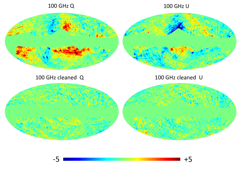
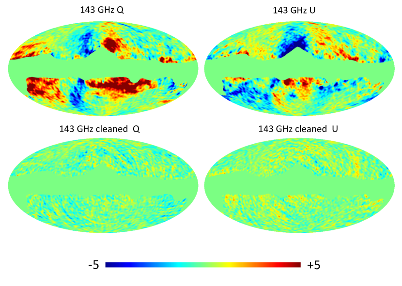
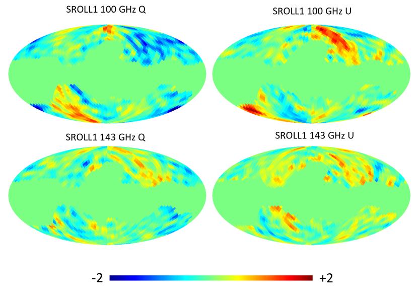
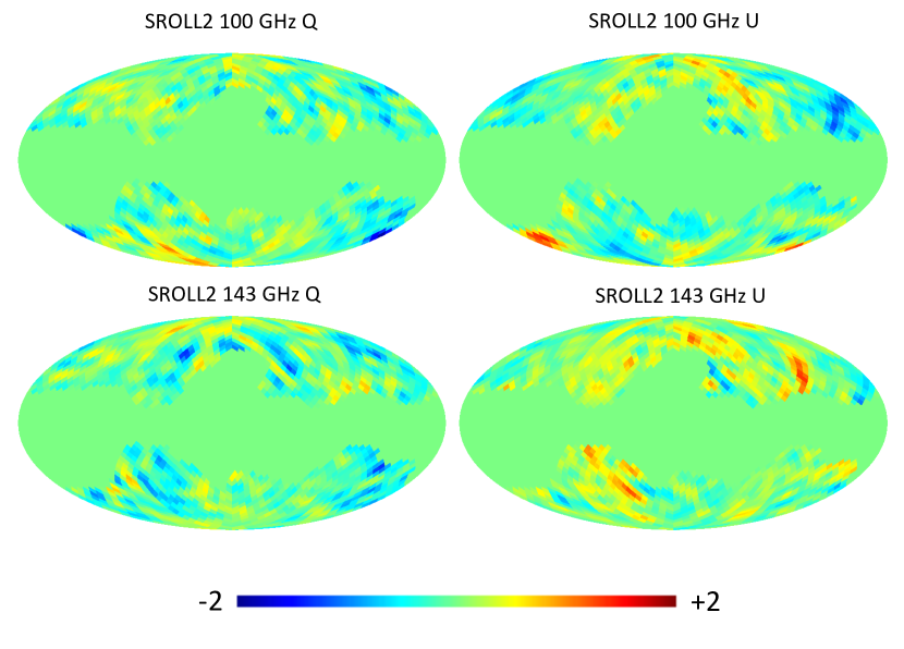
The SRoll2 polarisation maps before and after foreground cleaning are plotted in Fig. 2, which shows clearly that the polarisation maps at $100$ and $143$ GHz are dust dominated at low multipoles before foreground subtraction. Fig. 3 shows the foreground cleaned $N^{\rm lr}_{\rm side}=16$ $Q$ and $U$ maps used for the main cosmological results in this paper. The SRoll1 maps are shown in the upper panels and the SRoll2 maps are shown in the lower panels. One can clearly see systematic features in the SRoll1 maps, particularly at $100$ GHz. These systematic features can be reduced by subtracting a smoothed mean map $\mathbf{\bar{n}}$ determined from end-to-end simulations as discussed in the next section. For reference, the rms fluctuations in the SRoll2 $100$ GHz polarisation maps over the unmasked area shown in Fig. 3 are $\sigma^{P}=0.66\ \mu{\rm K}$ before foreground cleaning and $\sigma^{P}=0.36\ \mu{\rm K}$ after foreground cleaning. The rms of the scaled 353 GHz dust template is $\sigma^{P}=0.55\ \mu{\rm K}$ and for the scaled 30 GHz synchrotron template is $\sigma^{P}=0.11\ \mu{\rm K}$.

3.2 Noise covariance matrices

In this section, we describe how we fit a parametric model to estimates of the pixel-pixel noise covariance matrices (NCMs) computed from end-to-end simulations. Once we have a model for a NCM, we can generate large numbers of simulations on the assumption that the noise is Gaussian, allowing us to construct likelihoods as discussed in Sec. 4. We compute two sets of NCMs, one each for SRoll1 and SRoll2, from the end-to-end simulations of the map-making pipelines. In each case, the fiducial CMB and the input foreground model was subtracted, leaving maps containing noise and map-making systematics. We then construct empirical NCMs, $\mathbf{\hat{N}}$,

$$\mathbf{\hat{N}}=\frac{1}{n_{s}}\sum_{i=1}^{n_{s}}(\mathbf{n}_{i}-\mathbf{\bar{n}})(\mathbf{n}_{i}-\mathbf{\bar{n}})^{\top}\ ,$$ (23)

where $\mathbf{n}_{i}$ are the simulated sky maps for the Stokes parameters $T,Q$ and $U$, $\mathbf{\bar{n}}$ a smoothed template of the mean of the maps (see Eq. (30)) and $n_{s}$ the number of simulations used in the sum in Eq. (23). To test whether our methodology is biased as a consequence of overfitting we do not use all of the end-to-end simulations to compute Eq. (23). We excluded $100$ simulations from each set to allow validation tests of the likelihoods as discussed in Sec. 5.

We approach the problem of fitting a model to $\mathbf{\hat{N}}$ as a maximum likelihood inference problem. We assume a Gaussian probability distribution for each noise realisation

$$\mathcal{L}\equiv\mathbf{\mathcal{P}}(\mathbf{\hat{N}}|\mathcal{\mathbf{M}}) =\prod_{i=1}^{n_{s}}\frac{1}{\sqrt{|2\pi\mathbf{M}|}}e^{-\frac{1}{2}(\mathbf{n}_{i}-\mathbf{\bar{n}})\mathbf{M}^{\raisebox{0.43054pt}{$\scriptscriptstyle-1$}}(\mathbf{n}_{i}-\mathbf{\bar{n}})^{\top}}$$

$$=\frac{1}{|2\pi\mathbf{M}|^{\frac{n_{s}}{2}}}e^{-\frac{n_{s}}{2}\ \mathrm{tr}\ \mathbf{M}^{\raisebox{0.43054pt}{$\scriptscriptstyle-1$}}\mathbf{\hat{N}}}\ ,$$ (24)

where $\mathbf{M}$ is the model for the noise covariance matrix. We assume that $\mathbf{M}$ consists of three terms

$$\mathbf{M}=\alpha\mathbf{N}_{0}+\beta\mathbf{N}_{1}+\mathbf{Y\mathbf{\Psi}Y}^{\top},$$ (25)

where $\alpha$ and $\beta$ are scaling parameters for two matrices $\mathbf{N}_{0}$ and $\mathbf{N}_{1}$ and the term $\mathbf{Y\mathbf{\Psi}Y}^{\top}$ models large-scale modes with parameters $\mathbf{\Psi}$ as described more fully below. Since we are dealing with $Q$ and $U$ maps, the noise covariance matrices $\mathbf{M}$ are of size $(2N_{\rm pix},2N_{\rm pix})$. We neglect noise in temperature and only fit polarisation noise, since the low resolution $T$ maps are signal dominated to high accuracy. Moreover, we assume that the noise for $100$ and $143$ GHz maps is uncorrelated.

The matrices $\mathbf{N}_{0}$ are the $N^{\rm lr}_{\rm side}=16$ low resolution map-making covariance matrices (see e.g Tristram et al., 2011) computed for the parameters of the FFP8 simulations (Planck Collaboration, 2016a, b). These covariance matrices contain structure representing the scanning strategy, detector white noise and ‘$1/f$’-type noise, but do not include complexities associated with corrections for ADCNL. Since these matrices were designed to match the 2015 Planck half-mission maps, they do not necessarily match the noise levels of the SRoll1 and SRoll2 maps at high multipoles. The matrices $\mathbf{N}_{1}$ were constructed from the diagonal components ($(\sigma^{2})^{T}_{i}$, $(\sigma^{2})^{Q}_{i}$, $(\sigma^{2})^{U}_{i}$ of the $3\times 3$ $T,Q,U$ high resolution pixel noise estimates produced by the map-making algorithms. These noise estimates were degraded in resolution to $N^{\rm lr}_{\rm side}=16$ (appropriate for a low resolution map $X_{i}$) by computing:

$$\mathbf{N}_{\rm 1}\equiv\langle\mathbf{X}_{i}\mathbf{X}_{j}\rangle= \sum_{\ell_{1}\ell_{2}}\sum_{pq}\sigma^{2}_{p}\delta_{pq}\frac{(2\ell_{1}+1)}{4\pi}\frac{(2\ell_{2}+1)}{4\pi}\Omega_{p}\Omega_{q}$$

$$\qquad\times P_{\ell_{1}}(\cos{\theta_{ip}})P_{\ell_{2}}(\cos{\theta_{jq}})f_{\ell_{1}}f_{\ell_{2}}\ ,$$ (26)

for each $Q$ and $U$ (see App. A of Efstathiou et al. (2009)). We assume that the noise is diagonal $\langle x_{i}x_{j}\rangle=\sigma^{2}_{p}\delta_{pq}$, $\Omega_{i}$ is the solid angle of a high-resolution map pixel, $P_{\ell}$ denotes the Legendre polynomials and $f_{\ell_{i}}$ is the smoothing operator applied to the high-resolution maps given in Eq. (21). The sum

$$\mathbf{N}=\alpha\mathbf{N}_{0}+\beta\mathbf{N}_{1}$$ (27)

therefore allows us to model destriping noise correlations with adjustable ‘white noise’ levels, using the matrices $\mathbf{N}_{0}$ and $\mathbf{N}_{1}$ as templates.

The final term in Eq. (25) models additional large-scale noise correlations in the SRoll1 and SRoll2 end-to-end simulations. Terms up to $\ell_{\rm max}=4$ are added to the noise model via $\mathbf{Y}\mathbf{\Psi}\mathbf{Y}^{\top}$, where each column of the matrix $\mathbf{Y}$ is a map of the spherical harmonic functions $Y_{\ell m}(\theta,\varphi)$. The square matrix $\mathbf{\Psi}$, with dimensions equal to the number of large-scale modes that we wish to fit ($42$ modes to model $QQ$, $QU$ and $UU$ correlations), controls the covariance of the modes. In the noise fitting procedure we apply the binary polarisation mask with $f_{\rm sky}=0.54$, shown in Fig. 1, to the $Q$ and $U$ maps. This avoids fitting modes behind the Galactic plane.

To solve our inference problem, we minimise the ‘action’ $\mathcal{S}\equiv-\ln(\mathbf{\mathcal{P}}(\mathbf{\hat{N}}|\mathcal{\mathbf{M}}))$

$$\mathcal{S}=\frac{n_{s}}{2}\left(\ \mathrm{tr}\ \mathbf{M}^{\raisebox{0.60275pt}{$\scriptscriptstyle-1$}}\mathbf{\hat{N}}+\ln{|\mathbf{M}|}\right)\$$ (28)

with respect to the free parameters in our model for $\mathbf{M}$. We solve numerically for the scalar parameters $\alpha$ and $\beta$, solving analytically for the $\mathbf{\Psi}$ at each step. The matrix $\mathbf{\Psi}$ is given by (for the derivation see App. A)

$$\mathbf{\Psi}=(\mathbf{Y}^{\top}\mathbf{N}^{\raisebox{0.60275pt}{$\scriptscriptstyle-1$}}\mathbf{Y})^{\raisebox{0.60275pt}{$\scriptscriptstyle-1$}}\left(\mathbf{Y}^{\top}\mathbf{N}^{\raisebox{0.60275pt}{$\scriptscriptstyle-1$}}\left[\mathbf{\hat{N}}-\mathbf{M}\right]\mathbf{N}^{\raisebox{0.60275pt}{$\scriptscriptstyle-1$}}\mathbf{Y}\right)(\mathbf{Y}^{\top}\mathbf{N}^{\raisebox{0.60275pt}{$\scriptscriptstyle-1$}}\mathbf{Y})^{\raisebox{0.60275pt}{$\scriptscriptstyle-1$}}\ .$$ (29)

When fitting the NCM $\mathbf{M}$ using Eq. (25) the dominating components are the $1/f$-type noise matrix ($\alpha\approx 1.8$) as well as the large scale modes up to $\ell_{\rm max}=4$. The smoothed low resolution covariance matrix $\mathbf{N}_{\rm lr}$ only subtracted a small amount of power from the diagonal with $\beta\approx-0.1$.

As summarised in the start of this section, uncorrected ADCNL leads to ‘stripy’ residuals in the Planck $Q$ and $U$ maps at 100, 143, and 217 GHz, which are substantially reduced in SRoll2 compared to SRoll1 (see, for example, Fig. 4 in Pagano et al., 2020). The end-to-end simulations provide templates for these residuals. Instead of subtracting the mean map averaged over the simulations, $\bar{\mathbf{x}}$, we subtract a smoothed template

$$\bar{\mathbf{n}}=\mathbf{Y}(\mathbf{Y}^{\top}\mathbf{N}_{0}^{\raisebox{0.60275pt}{$\scriptscriptstyle-1$}}\mathbf{Y})^{\raisebox{0.60275pt}{$\scriptscriptstyle-1$}}\mathbf{Y}^{\top}\mathbf{N}_{0}^{\raisebox{0.60275pt}{$\scriptscriptstyle-1$}}\bar{\mathbf{x}}\ ,$$ (30)

with $\ell_{\rm max}=4$ (this is the maximum likelihood solution of the map-making equation, as discussed in e.g. Tegmark (1997b)). We have approximated the NCM in Eq. (30) by the term $\mathbf{N_{0}}$ to avoid having to iterate to obtain a solution for $\mathbf{M}$.

3.3 Quadratic temperature and polarisation power spectra

Figure 4: Low-$\ell$ QCS estimates for $100\times 143$ temperature ($TT$, $TE$) and polarisation ($EE$, $BB$) full-mission cross-spectra of SRoll2 (red) and Planck 2018 (blue) maps with $\mathcal{D}_{\ell}=\ell(\ell+1)C_{\ell}/(2\pi)$. The COMMANDER 2018 $TT$ cross-spectrum (PCP18) (dotted lined) with the associated error bar as a grey shaded region is shown for comparison. The maps are foreground cleaned with the 30 GHz and 353 GHz channel for synchrotron and dust emission, respectively. Theoretical spectra are shown for $\tau=0.055$ (solid line) and $\tau=0.070$ (dashed line).

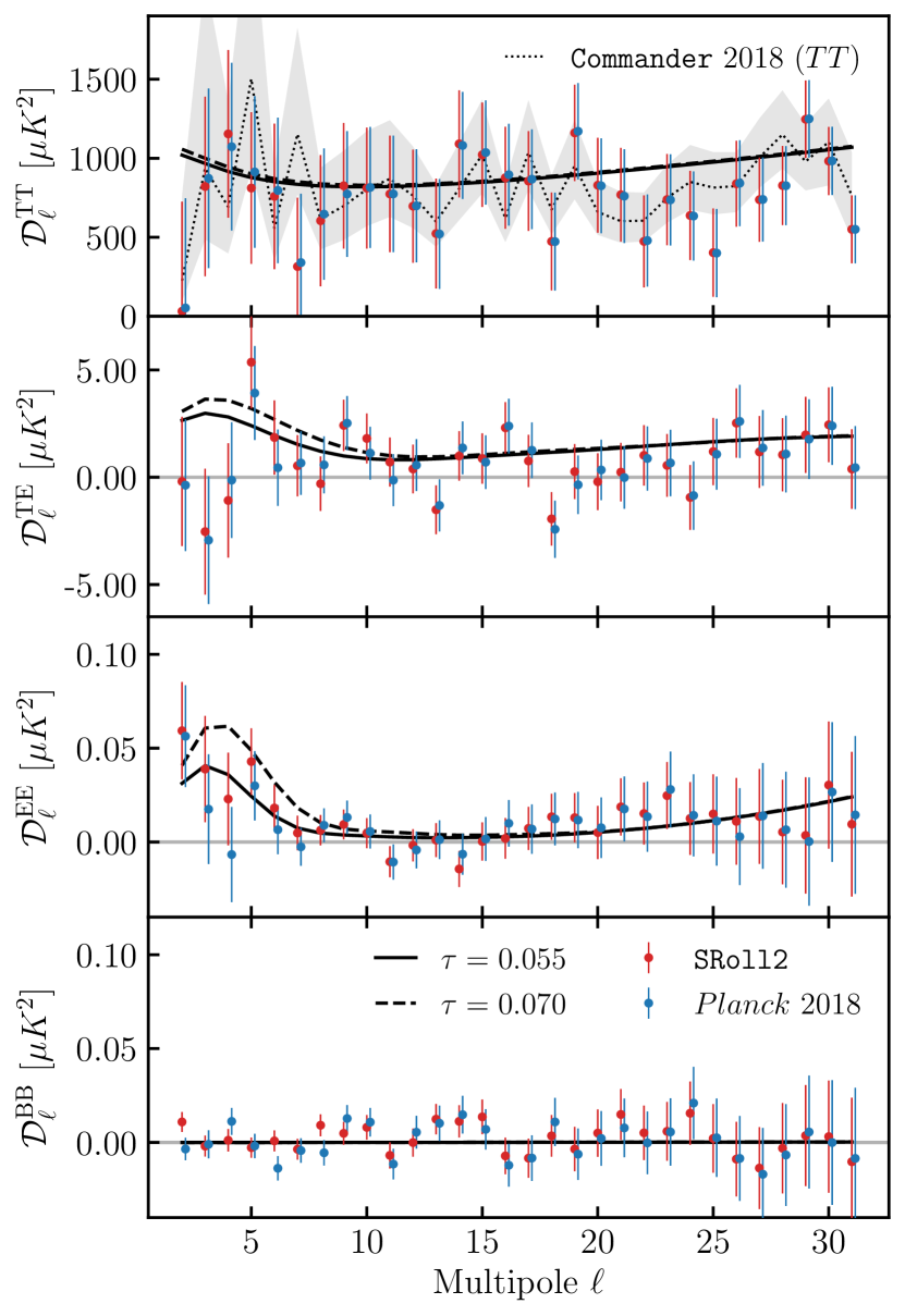
As an illustration of our methods, Fig. 4 shows the $TT$, $TE$, $EE$ and $BB$ spectra, computed using the QCS estimator technique presented in Sec. 2, for the cross correlation of the $100$ and $143$ GHz full-mission maps for both SRoll1 and SRoll2 for $2\leq\ell\leq 31$. The $T$, $Q$ and $U$ maps have been foreground cleaned as discussed in Sec. 3.1. We apply a mask with $f_{\rm sky}=0.70$, shown in Fig. 1, to the $T$ maps and we apply a mask with $f_{\rm sky}=0.54$, also shown in Fig. 1, to the $Q$ and $U$ maps. For the $TT$ cross-spectra we compare our results with the COMMANDER 2018 spectrum (PCP18) and observe good agreement between them, even though the COMMANDER $TT$ spectrum is computed using a mask with larger sky fraction ($f_{\rm sky}=0.86$). In particular, we observe the same behaviour in the spectra: first, at $\ell=2$ there is a very low value, and, second, there is a ‘dip’ at around $\ell\simeq 20-25$. The error bars on the COMMANDER spectrum are asymmetric $1\sigma$ posterior widths.

To guide the eye, the solid and dashed black lines in Fig. 4 show the $TT$, $TE$ and $EE$ spectra for base $\Lambda$CDM model with $\tau=0.055$, close to the best fit value for the SRoll1 and SRoll2 maps cited in Eqs. (3a) and (3b), and for $\tau=0.070$, which is disfavoured at about the $2-3\sigma$ level. The $TT$ and $TE$ spectra have large cosmic variance and so do not provide strong constraints on $\tau$ given the low values of $\tau$ inferred from the $EE$ spectra. The SRoll1 and SRoll2 $TT$, $TE$ and $EE$ spectra are very similar and mainly show differences at low multipoles. The $BB$ spectra are approximately consistent with zero, providing an important null-test for SRoll1 and SRoll2. The $\chi^{2}$ values divided by the degrees of freedom (29 multipoles) are 1.28 for SRoll1 and 1.13 for SRoll2.

Figure 5: Low-$\ell$ QCS estimates for $TT$, $TE$, $EE$ and $BB$ auto- and cross-spectra of detector set combinations for 100 and 143 GHz low-resolution SRoll2 maps with $\mathcal{D}_{\ell}=\ell(\ell+1)C_{\ell}/(2\pi)$. The maps are foreground cleaned with the 30 GHz and 353 GHz channels for synchrotron and dust emission, respectively. Theoretical spectra are shown for $\tau=0.055$ (solid line) and $\tau=0.070$ (dashed line). For comparison, the black circles show the $100\times 143$ full-mission QCS estimates with corresponding error bars.

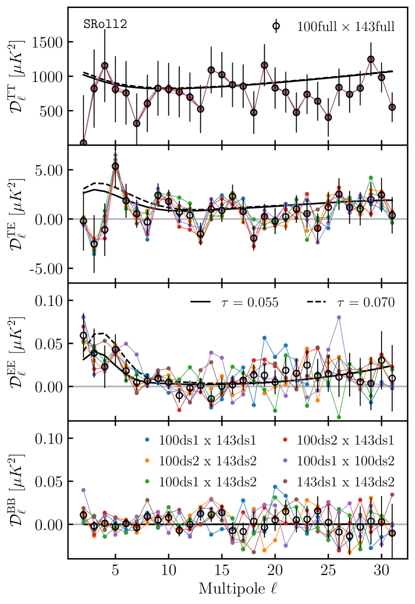
Fig. 5 shows $TT$, $TE$, $EE$ and $BB$ spectra computed using the QCS scheme for intra- and inter-frequency cross-spectra for combinations of the publicly available SRoll2 detector set maps. The $T$, $Q$ and $U$ maps are foreground cleaned, following the procedure discussed in Sec. 3, i.e. the ds1 maps are cleaned using 353 GHz HM1 and 30 GHz HM1 maps and the ds2 maps are cleaned with 353 GHz HM2 and 30 GHz HM2 maps. The temperature and polarisation masks are the same as those used as for the previously discussed full-mission cross-spectra and shown in Fig. 1. For comparison, the empty black circles are the $100\times 143$ full-mission QCS estimates with the corresponding error bars (as in Fig. 4).

For the signal-dominated $TT$ and $TE$ cases seen in Fig. 5, we measure almost identical spectra for the different detector set combinations as expected. In the low multipole $EE$ polarisation regime that is most constraining for $\tau$ ($2\leq\ell\lesssim 12$), the estimates scatter between the theoretical curves with $\tau=0.055$ and $\tau=0.070$. This indicates that higher values of $\tau$ may be favoured for some detector set combinations. At intermediate scales, $10\leq\ell\leq 25$, the spectra scatter around the theoretical curves and no clear trend is visible. However, the $100\ \mathrm{ds1}\times 100\ \mathrm{ds2}$ intra-frequency cross spectrum shows a few outliers in polarisation (purple line). This potentially suggests that the 100 GHz maps are more affected by noise and unresolved systematics than the 143 GHz ones. The illustrated $BB$ spectra are all approximately consistent with the null hypothesis of zero signal power.

4 Likelihoods

In this section we present and compare a simulation-based likelihood, a likelihood-approximation scheme and a likelihood-free approach. The methods are called: SimBaL, glass and delfi and their respective likelihoods are named C-SimLow , momento and pydelfi.

4.1 Simulation-based likelihood

The simulation-based likelihood (SimBaL), originally presented in PSRoll1, uses low-$\ell$ QCS estimates of only the $EE$ polarisation spectrum to measure the optical depth.

The joint sampling distribution for all the power spectrum elements is in general a function of all the power spectra components defining the model. However, the QCS procedure with reshaping, see Eq. (7), does a good job of approximately factorising this distribution by multipole. Then the distribution of the power spectrum elements at a given multipole depends mainly on the theory elements at that multipole. By only considering a single spectrum, $EE$ in this case, the requirement to handle intra-multipole correlations is avoided, motivating an approximate likelihood form:

$$\mathcal{L}(\mathbf{C}|\mathbf{\hat{C}})=\prod_{\ell=\ell_{\rm min}}^{\ell_{\rm max}}\mathcal{L}_{\ell}(C_{\ell}|\hat{C}_{\ell})\ ,$$ (31)

with $\ell_{\rm min}=2$ and $\ell_{\rm max}=29$, a product of one-dimensional functions.

One then uses realisations generated according to a set of theory models to fit parametric forms to each of these one-dimensional sampling distributions. This is done for each $\ell$ at the input theory $C_{\ell}$ values that happen to occur in the models considered. These fits are then evaluated at a realised $C_{\ell}$ value set equal to that of the real data $\hat{C}_{\ell}$. Finally, a further fit to these numbers, now as a function of the theory $C_{l}$, gives the effective likelihood function at that multipole.

As the mask and noise do correlate the multipoles even with QCS, one may ask where such effects manifest themselves in the above procedure. At a given $\ell=\ell_{0}$ say, one can imagine computing the marginalised one-dimensional sampling distribution for $\hat{C}_{\ell_{0}}$ for a specific theory power spectrum. Because of the couplings, in general this will differ between models even if they happen to share the same value of $C_{\ell_{0}}$. The fitting procedure above then effectively averages over these distributions. One expects the variations to be relatively modest for plausible models, and hopes that the theory models used to generate the realisations are close enough to reality not to lead to significant errors in the effective averaging.

We therefore need to generate full maps of the observed CMB on which to measure the spectra. Considering the theory $C_{\ell}$’s for each mode over a large region of the parameter space would be computationally costly, since one would typically spend much time exploring low probability regions. We thus only explore the region of the power spectrum around the theory $C_{\ell}$ of interest.

Our implementation of the simulation-based likelihood largely follows that of Planck Collaboration (2020c). The main difference is that we use Gaussian realisations of our noise fit to the Planck simulations, rather than using the outputs of the noise simulations directly, given the limited number of the latter. This allows us to use many more independent noise realisations throughout the procedure.

We generate 191 theoretical power spectra, $C_{\ell}(\tau,\theta)$, uniformly sampled over a range of $\tau$ values from $0.01-0.2$ inclusive with a step size of $\Delta\tau=0.001$, where $\theta$ denotes all the cosmological model parameters defined in Sec. 6. Only $A_{s}$ is varied along with $\tau$, to keep the product $10^{9}A_{s}e^{-2\tau}$ fixed at $1.870$, consistent with a high-$\ell$ likelihood constraint. For each of these theoretical power spectra, we generate 10000 Monte Carlo realisations of the CMB. Using the fitted NCM discussed in Sec. 3.2, we generate Gaussian noise realisations that capture noise and systematics for the relevant frequency and detector set maps. At the map level, we combine the signal and noise maps. With this large suite of simulations we set up the simulation-based likelihood in the following way:

1. Compute low-$\ell$ QCS estimates of the simulations, $\hat{C}_{\ell}^{\rm sim}$, from given theory power spectra that have values $C_{\ell}$.

2. Compute the quasi-conditional $\mathcal{P}(\hat{C}_{\ell}^{\rm sim}|C_{\ell})$ by fitting $\ell$-by-$\ell$ a model to the distribution of spectra. We perform an unbinned maximum likelihood fit to the log-distribution, $\ln{\mathcal{P}(\hat{C}_{\ell}^{\rm sim}|C_{\ell})}$ as a function of $\hat{C}_{\ell}^{\rm sim}$, using a third-order polynomial for the central part of the distribution and a first-order polynomial for its tails. Using Lagrange multipliers, we impose smoothness and continuity at the boundaries ensuring a good fit, $f_{\ell}(\hat{C}_{\ell}^{\rm sim}|C_{\ell})$, to the conditional.

3. We evaluate the above fits across the models at $\hat{C}_{\ell}$, the QCS spectra for the data, fitting the same functional form as that used above but this time for the $C_{\ell}$ dependence.

4. Finally we construct our likelihood by combining the fits for each multipole as given in Eq. (31), yielding

   $$\ln\mathcal{P}(\mathbf{\hat{C}}|\mathbf{C})=\sum_{\ell=2}^{29}\ln f_{\ell}(\hat{C}_{\ell}|C_{\ell})\ .$$ (32)

The method will be called SimBaL throughout the paper and we shall denote our implementation of it by C-SimLow. In the present paper, we use C-SimLow with only polarisation data for the reason discussed above of the difficulties in handling correlations between variables.

4.2 Likelihood approximation scheme

The General Likelihood Approximate Solution Scheme (glass; Gratton, 2017) was developed to allow a principled Bayesian analysis of data even in situations where the sampling distribution for the data is not fully known. Our low-$\ell$ analysis of the CMB polarisation is a case in point – because of difficulties in quantifying the noise in the maps, we choose to use quadratic cross-spectra for robustness. However, the joint distribution of the multipoles of such spectra, computed on a masked sky, does not have a simple analytic form. Instead, glass assumes one can compute certain moments of functions of the data, here the spectral multipoles, as a function of the parameters of the model under investigation. One can then imagine glass uses a maximum entropy construction to compute a least-presumptive sampling distribution consistent with these moments. We now introduce the method, briefly summarising Gratton (2017), to which the reader is referred for a fuller presentation.

For an initial illustration, consider a situation in which one can obtain the mean $\bar{x}(q)$ and variance $\sigma^{2}_{x}(q)$ of some function of the data $x$ in terms of a model parameter $q$, ideally analytically but also potentially via forward simulations. Then, one maximises the entropy of the system

$$H(\mathcal{P})=-\int\mathrm{d}x\ \mathcal{P}(x)\ln{\frac{\mathcal{P}(x)}{\pi(x)}}\$$ (33)

subject to the constraints on $\bar{x}(q)$, $\sigma^{2}(q)$ and normalisation of $\mathcal{P}(x)$, imposed via Lagrange multipliers. The required values of the multipliers, $\lambda_{x}(q)$ and $\lambda_{xx}(q)$, may be solved for, in general numerically, as a function of $q$. The sampling distribution is then given as

$$\mathcal{P}(x)=\frac{\pi(x)e^{-\lambda_{x}x-\lambda_{xx}x^{2}}}{\int dx\pi(x)e^{-\lambda_{x}x-\lambda_{xx}x^{2}}}=\frac{1}{\mathcal{Z}}\pi(x)e^{-\lambda_{x}x-\lambda_{xx}x^{2}}\ ,$$ (34)

where $\mathcal{Z}$ is a theory-dependent normalisation constant (also called the evidence or partition function).

Equivalently, this can be understood as solving for the action (or negative log-likelihood) $\mathcal{S}$,

$$\mathcal{S}(x,q)=-\ln{\pi(x)}+\lambda_{x}(q)x+\lambda_{xx}(q)x^{2}+\ln{\mathcal{Z}(\lambda(q))}\ .$$ (35)

The method naturally extends to multiple statistics $x^{i},\ i\in\mathopen{[}1,\dots,n\mathclose{]}$ fitted to models with multiple parameters $q^{\alpha},\ \alpha\in\mathopen{[}1,\dots,m\mathclose{]}$, and using higher moments:

$$\mathcal{S}(x,q) =-\ln{\pi(x)}+\lambda_{i}x^{i}+\lambda_{ij}x^{i}x^{j}+$$ (36)

$$\qquad+\lambda_{ijk}x^{i}x^{j}x^{k}+\dots+\ln{\mathcal{Z}(\lambda(q^{\alpha}))}\ ,$$

where summation is implied over multiple indices.

However, the evaluation of the Lagrange multipliers quickly becomes very expensive, requiring the numerical computation of many multi-dimensional integrals. We can avoid this cost by instead computing more moments. To simplify notation, we introduce a ‘meta-index’ $I$ to first run over all indices $i$, then all pairs of indices $ij$, and so on. $X^{I}$ then runs over the $x^{i}$, then the $x^{i}x^{j}$ and so on, and similarly $\lambda_{I}$ runs over the $\lambda_{i}$, then the $\lambda_{ij}$ and so on. We can express the moments of the $X^{I}$ as derivatives of the evidence $\mathcal{Z}$ with respect to the Lagrange multipliers:

$$\langle X^{I}\rangle(\lambda) =-\frac{\partial\ln\mathcal{Z}}{\partial\lambda_{I}}\ ,$$ (37)

$$\langle\langle X^{I}X^{J}\rangle\rangle(\lambda) =\frac{\partial^{2}\ln\mathcal{Z}}{\partial\lambda_{I}\partial\lambda_{J}}\ .$$ (38)

Next, we differentiate Eq. (37) with respect to $q^{\alpha}$

$$\langle X^{I}\rangle_{,a}=-\frac{\partial^{2}\ln\mathcal{Z}}{\partial\lambda_{J}\partial\lambda_{I}}\frac{\partial\lambda_{J}}{\partial q^{\alpha}}=-\langle\langle X^{I}X^{J}\rangle\rangle\lambda_{J_{,a}}.$$ (39)

Now, differentiating the action in Eq. (36) yields

$$\mathcal{S}_{,a}=(X^{I}-\langle X^{I}\rangle)\lambda_{J_{,a}}\ .$$ (40)

We can solve Eq. (39) for the $\lambda_{J_{,a}}$ in terms of the derivatives of the first moments and second order cumulants. Substituting into (40), and adopting a vector/matrix notation to avoid explicitly writing meta-indices, we obtain

$$\mathcal{S}_{,a}=-(X-\langle X^{\top}\rangle)\langle\langle XX^{\top}\rangle\rangle^{\raisebox{0.60275pt}{$\scriptscriptstyle-1$}}\langle X\rangle_{,a}\ ,$$ (41)

which does not depend explicitly on the prior and the Lagrange multipliers. So, obtaining the moments by calculation or simulations, we can compute the gradient of $\mathcal{S}$. This gradient can then subsequently be integrated between two points in parameter space in order to find the difference in approximate log-likelihood between the two models.

For an instructive if overly simple example, consider applying the above procedure in a 1-d problem in which the prior $\pi(x)$ is uniform and the first two moments of $x$ happen to be calculable as $\langle x\rangle=\mu$ and $\langle x^{2}\rangle=\mu^{2}+\sigma^{2}$, where $\mu$ is a variable parameter of the model and $\sigma^{2}$ is fixed. Assume we will work to linear order in $x$ for $\mathcal{S}$. $I$ then ranges over just one element, with $X^{0}$ simply being $x$. Knowing up to second moments in $x$ is then sufficient to evaluate the single component of $\langle\langle XX^{\top}\rangle\rangle$, which is $\langle x^{2}\rangle-\langle x\rangle^{2}=\sigma^{2}$. Eq. (41) simply reads

$$\mathcal{S}_{,\mu}=-(x-\mu)\frac{1}{\sigma^{2}}\cdot 1$$ (42)

which in this case we can integrate by inspection to find $\mathcal{S}=(x\mu-\mu^{2}/2)/\sigma^{2}$ up to a constant. For inference of $\mu$ this of course may be rewritten as $\mathcal{S}=(x-\mu)^{2}/(2\sigma^{2})+\mathrm{const}$, the exact Gaussian result that one might have anticipated from the form of the moments.

For a more complicated example, consider observing a number of vectors $\mathbf{y}$ of Gaussian-distributed components, with the vectors being independent of each other but allowing components within a single vector to be correlated with each other according to a covariance matrix $\mathbf{C}$. The sampling distribution is then

$$\mathcal{P}(y|\mathbf{C})\mathop{}\!\mathrm{d}^{2\ell+1}y=\frac{\mathop{}\!\mathrm{d}^{2\ell+1}y}{|2\pi\mathbf{C}|^{(2\ell+1)/2}}e^{-\frac{1}{2}\sum_{i}y_{i}^{\top}\mathbf{C}^{\raisebox{0.43054pt}{$\scriptscriptstyle-1$}}y_{i}}\ ,$$ (43)

and we see that the components of the observed covariance matrix $\hat{\mathbf{C}}$,

$$\hat{\mathbf{C}}\equiv\frac{1}{2\ell+1}\sum_{i}y_{i}y_{i}^{\top}\ ,$$ (44)

serve as sufficient statistics for learning about the components of $\mathbf{C}$. The glass scheme recovers the posterior associated with (43) simply by working to linear order in the components of $\hat{\mathbf{C}}$ for $\mathcal{S}$: after calculating their first and second moments, with some work Eq. (41) recovers the optimal result

$$\mathcal{S}_{\mathrm{true}}=\left(\ell+\frac{1}{2}\right)\left(\ \mathrm{tr}\ \mathbf{C}^{\raisebox{0.60275pt}{$\scriptscriptstyle-1$}}\hat{\mathbf{C}}+\ln{\frac{|\mathbf{C}|}{|\hat{\mathbf{C}}|}}-1\right)\ .$$ (45)

Hence we see how to use glass to compute an approximate likelihood, which we name momento, for the cross-spectra in our problem. One can in principle compute all of the intra- and inter- $\ell$ cumulants between all the (TT, TE and) EE cross-spectra up to some required degree of approximation, assuming the underlying maps are gaussianly-distributed (around some offset noise template). In practice this is relatively easily manageable up to fourth order in the spectra for moderate $\ell_{\mathrm{max}}$. Such moments are the natural generalisations of the following formulae for a single multipole of a single cross spectrum $\hat{C}_{12}$ on the full sky with isotropic noise (and no unsubtracted map mean noise template):

$$\langle\hat{C}_{12}\rangle =C\ ,$$ (46)

$$(2l+1)\langle\langle\hat{C}_{12}^{2}\rangle\rangle =C^{2}+(C+N_{11})(C+N_{22})\ ,$$ (47)

$$(2l+1)^{2}\langle\langle\hat{C}_{12}^{3}\rangle\rangle =2C^{3}+6C(C+N_{11})(C+N_{22})\ ,$$ (48)

$$(2l+1)^{3}\langle\langle\hat{C}_{12}^{4}\rangle\rangle =6\left(C^{4}+(C+N_{11})^{2}(C+N_{22})^{2}\right.$$

$$\qquad\left.+\ 6C^{2}(C+N_{11})(C+N_{22})\right)\ .$$ (49)

Taking the theory power components themselves as parameters of the theory, using such cumulants we can numerically integrate $\mathcal{S}_{,a}$ up along a path from a fiducial model to a model in question, for a selection of degrees of approximation (linear and quadratic, requiring from quadratic up to fourth order moments of the spectra). We find that even the linear approximation performs well and so typically use this in our work.

To summarise, momento uses QCS power spectra, which use a reasonable fiducial model with power spectrum $C_{\ell}^{\mathrm{fid}}$ to construct the appropriate matrices. Then, for each likelihood evaluation, momento:

1. takes as input a set of theory $C_{\ell}$’s,

2. computes the difference $\Delta C_{\ell}\equiv C_{\ell}-C_{\ell}^{\mathrm{fid}}$ between the theory and the fiducial model

3. uses Romberg integration to compute the change in $\mathcal{S}$ going from the fiducial $C_{\ell}^{\mathrm{fid}}$’s to the theory $C_{\ell}$’s along the line $C_{\ell}^{\mathrm{fid}}+a\Delta C_{\ell}$ in power spectrum space, with $a$ being a parameter ranging from zero to one. We choose to use a step size in $a$ of $0.25$.

4. This requires the computation of gradients of $\mathcal{S}$ with respect to $a$ at four new positions in power spectrum space for every new likelihood evaluation (at $a=0.25,0.5,0.75,1$), as those computed at the fiducial model ($a=0$) can be reused.

5. The gradients of $\mathcal{S}$ with respect to $a$ are linear combinations of those of $\mathcal{S}$ with respect to the associated $C_{\ell}$’s, and

6. these $\partial\mathcal{S}/\partial C_{\ell}$’s are computed via Eq. (41), which require both the QCS power spectra of the data and

7. the multidimensional moments/cumulants of the QCS power spectra evaluated at the theory model corresponding to each $a$, via the appropriate multidimensional generalisations of Eqs. (46) - (47) in quick ‘linear’ mode or Eqs. (46) - (49) in the fuller ‘quadratic’ mode.

In general, glass is a very flexible scheme to compute principled posteriors where likelihoods are challenging to compute either for computational efficiency or more fundamental reasons. Since the approach is physically motivated, we do not have the ‘black box’ behaviour seen in delfi or other neural-network-based approaches. In contrast to the two other methods, which are dependent on the use of simulations to train their models, momento only needs simulations for the computation of suitable NCMs, which are then used in the computation of moments as required.

4.3 Density-estimation likelihood-free inference

The final method takes an alternative approach to perform a simulation-based likelihood and is called the ‘likelihood-free’ approach. In Sec. 4.1 we fit a functional form to the likelihood $\mathcal{L}(C_{\ell}|\hat{C}_{\ell})$ and obtained a total likelihood by assuming that each $\ell$ is independent. In this section we instead seek an invertible remapping of the measured cross-spectra, $\hat{C}_{\ell}$, to a set of variables $u_{\ell}$, such that the resulting variables are statistically independent, Gaussian random variables. This mapping is obtained using a neural network (NN). With such a mapping the likelihood can be trivially evaluated as it is a multidimensional Gaussian combined with an appropriate Jacobian. The challenge with this approach is to obtain the mapping when the functional form of the distribution of the $\hat{C}_{\ell}$ is unknown.

More precisely, we start with a set of $N$ variables, $u_{\ell}$, that are unit-variance normal variables when conditioned on the parameters, i.e. $u_{\ell}|\mathbf{\theta}\sim\mathcal{N}(0,I)$, where $\mathbf{\theta}$ denotes the conditional parameters (in our case $\tau$). We wish to find an invertible function such that $\hat{C}_{\ell}=f(u_{\ell})$. Given such a mapping we see that

$$\mathcal{P}(\hat{C}_{\ell}|\theta)\mathrm{d}^{N}\hat{C}_{\ell} =\mathcal{P}(f(u_{\ell})|\theta)\left|\frac{\partial\hat{C}_{\ell}}{\partial u_{\ell}}\right|\mathrm{d}^{N}u_{\ell}$$

$$=\mathcal{P}_{u}(u_{\ell}|\theta)\mathrm{d}^{N}u_{\ell}\ ,$$ (50)

where the density for $u_{\ell}$, $\mathcal{P}_{u}(u_{\ell}|\theta)$, is just a normal distribution. Finding the mapping $f(u_{\ell})$, with a tractable Jacobian, seems a daunting task in general; the mapping from the $N$-dimensional normal distribution to potentially multimodal distributions is likely non-trivial. To solve this challenge we use a second technique: the above remapping can be expressed as a series of $D$ simpler mappings, i.e.

$$\hat{C}_{\ell}=f(u_{\ell})=f_{D}(f_{D-1}(\dots f_{1}(u_{\ell})))$$ (51)

with the only modification that Eq. (4.3) is changed to a product of Jacobians. The intuition is that we decompose the complex mapping into a series of simple transformations that slowly deform the probability density into a distribution that approaches that of the complex mapping. We consider a particularly simple series of mappings. For the j^th mapping we perform the following transformation:

$$f_{j}^{i}(\mathbf{x}|\theta)=\frac{\mathbf{x}^{i}-\mu^{i}_{j}(\mathbf{x}^{1...i-1},\theta)}{\sigma^{i}_{j}(\mathbf{x}^{1...i-1},\theta)}\ ,$$ (52)

i.e. that the $i^{\mathrm{th}}$ output of the mapping is obtained by subtracting and scaling the $i^{\mathrm{th}}$ input by a function of all the previous ($i-1$) inputs. This has the nice property that the Jacobian in Eq. (4.3) for each transformation has the trivial form of the product of the functions $\sigma^{i}_{j}(x^{1...i-1},\theta)$ . Thus, the desired distribution can be written as

$$\mathcal{P}(\hat{C}_{\ell}|\theta)\mathrm{d}^{N}\hat{C}_{\ell}=\mathcal{P}(u_{\ell}|\theta)\prod\limits_{j=1}^{D}\prod\limits_{i=1}^{N}\sigma^{i}_{j}(u_{\ell},\theta)\,\mathrm{d}^{N}u_{\ell}\ .$$ (53)

This expression of the problem has shifted the complexity from fitting a functional form for the likelihood to identifying a suitable series of mapping functions $\sigma^{i}_{j}(u_{\ell};\theta)$.

To proceed we consider a family of functions $\sigma^{i}_{j}(u_{\ell},\theta|\mathbf{w})$, parametrised by $\mathbf{w}$, and optimise the parameters to find the appropriate mapping. Equivalently stated, we solve a variational inference problem: we have a parametrised form for the likelihood $\mathcal{P}(\hat{C}_{\ell}|\theta;\mathbf{w})$ and we wish to optimise the parameters so that we can approximate the true likelihood as accurately as possible.

To find the best fitting weights of the NN, we minimise the Kullback-Leibler divergence $D_{\rm KL}(\mathcal{P}^{*}|\mathcal{P})$, between the parametric distribution $\mathcal{P}(\hat{C}_{\ell}|\theta;\mathbf{w})$ and the true distribution $\mathcal{P}^{*}(\hat{C}_{\ell}|\theta)$, which is defined as

$$D_{\rm KL}(\mathcal{P}^{*}|\mathcal{P})=-\int\mathcal{P}^{*}(\hat{C}_{\ell}|\theta)\ln\frac{\mathcal{P}(\hat{C}_{\ell}|\theta;\mathbf{w})}{\mathcal{P}^{*}(\hat{C}_{\ell}|\theta)}\mathrm{d}^{N}{\hat{C}}_{\ell}\ .$$ (54)

The Kullback-Leibler divergence is a measure of the difference between probability distributions; it is a non-negative function that is zero only when the two distributions are identical. By minimising this function, we minimise the mismatch between our parametric conditional distribution and the true conditional distribution.

As we do not have access to the true distribution, only samples, we perform a Monte Carlo approximation of the Kullback-Leibler divergence using

$$D^{\rm Monte\ Carlo}_{\rm KL}(\mathcal{P}^{*}|\mathcal{P})=-\sum_{i=1}^{N_{\rm samples}}\ln{\mathcal{P}(\hat{C}_{\ell}|\theta;\mathbf{w}}),$$ (55)

which, as the number of samples tends to infinity, approaches Eq. (54) up to an additive constant.

In principle, any family of functions can be used to perform the parametric fitting in this approach. However, if an overly restrictive set of functions is chosen we will have a poor approximation of the true distribution. Thus, in this work we choose the set of functions to be representable by a NN. NN are universal approximators, thus given sufficient data they can represent any function meaning we have a sufficiently flexible class of functions.

We use the pydelfi implementation of this method to construct a polarisation-only and a joint temperature-polarisation likelihood, with the precise configuration shown in App. C. When dealing with a high-dimensional problem ($D\lower 2.15277pt\hbox{$\;\buildrel>\over{\sim}\;$}30$) in likelihood-free-inference, score compression is required both to reduce computational cost and give stable results. The greater the degree of compression, the more sub-optimal the likelihood. As a consequence, the results of our $TTTEEE$ pydelfi likelihood have larger uncertainties, as discussed in detail in App. C.3 (for a more general discussion, see Alsing et al. (2018)).

5 Likelihood validation on simulations

Figure 6: A test of the three likelihoods (C-SimLow, momento and pydelfi) on 100 simulated signal maps with an input $\tau=0.060$ and 100 noise and systematics maps from the SRoll2 end-to-end simulations. Each posterior per simulation is shown in black and the dashed black line is the mean of the maximum likelihood values for each method. The $\tau$ value in each top right corner shows the mean of the maximum likelihood values for $\tau$ over the simulations and the mean of the posterior widths.

Figure 7: Scatter plots between the maximum likelihood values corresponding to the posteriors shown in Fig. 6 for the three pairs of the likelihood methods (C-SimLow, momento and pydelfi). The grey shaded area shows the typical posterior width for the optical depth $\sigma(\tau)$. The black, red and green dashed lines show linear fits to each set of points. Their correlation coefficients (slopes of the linear fit) are given in the legend. There is a high degree of correlation between all three methods, especially between C-SimLow and pydelfi.

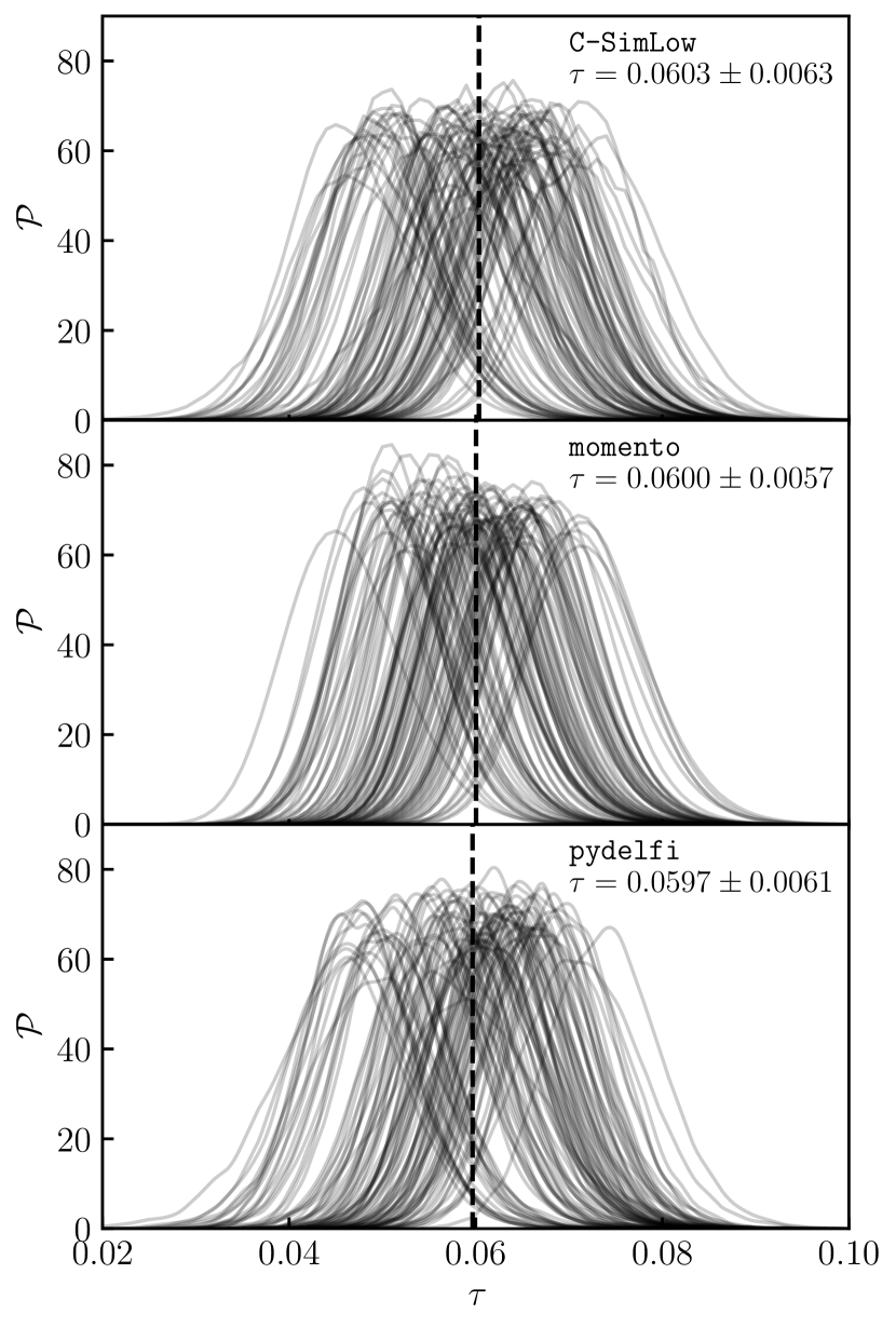
In this section we present tests of the three likelihood methods discussed in Sec. 4 against simulations. The aim is to investigate whether there are biases or significant differences in their performance. We also test what happens if the input value of $\tau$ in the simulations is changed to be higher or lower than the fiducial value of $0.06$ used to construct the covariance matrices required for the QCS estimator.

Since end-to-end simulations are used to model noise, we have taken care to use an independent subset of the simulations for the tests described in this section. Thus, the noise estimation steps used all but 100 end-to-end simulations for each SRoll1 and SRoll2, leaving the remaining simulations available for likelihood validation. We also generated 100 new Gaussian CMB realisations for each of three values of $\tau$: $\tau=0.05$, $0.06$ and $0.07$, using the same CMB realisations for SRoll1 and SRoll2. We use the same masks for the tests as for the data analysis (illustrated in Fig. 1).

Fig. 6 compares the performance of the three likelihood methods for polarisation-only ($EE$) inferences on $\tau$ for the SRoll2 simulations (the SRoll1 case is very similar). The figure shows posteriors for each of the 100 test simulations using the $\tau=0.06$ CMB realisations. All three likelihoods perform satisfactorily, without significant bias. The mean maximum likelihood values $\overline{\tau_{\rm ML}}$, mean of the posterior widths $\overline{\sigma(\tau)}$ and the standard deviation of the maximum likelihood values $\sigma(\tau_{\rm ML})$ found for each likelihood are given in Table 2 (which also lists values for the $\tau=0.05$ and $0.07$ CMB realisations).

Likelihoods	$\tau_{\rm in}=0.050$			$\tau_{\rm in}=0.060$			$\tau_{\rm in}=0.070$
	$\overline{\tau_{\rm ML}}$	$\overline{\sigma(\tau)}$	$\sigma(\tau_{\rm ML})$	$\overline{\tau_{\rm ML}}$	$\overline{\sigma(\tau)}$	$\sigma(\tau_{\rm ML})$	$\overline{\tau_{\rm ML}}$	$\overline{\sigma(\tau)}$	$\sigma(\tau_{\rm ML})$
C-SimLow	0.0503	0.0064	0.0077	0.0603	0.0063	0.0069	0.0703	0.0063	0.0066
momento	0.0498	0.0056	0.0063	0.0600	0.0057	0.0063	0.0704	0.0060	0.0065
pydelfi	0.0496	0.0064	0.0077	0.0597	0.0060	0.0068	0.0697	0.0058	0.0065

Table 2: Summary of likelihood tests performed using Gaussian realisations of CMB signal maps and 100 end-to-end SRoll2 simulations for the simulation-based likelihood (C-SimLow), the likelihood approximation scheme (momento) and the density-estimation likelihood-free (pydelfi) method. Here we make inferences on $\tau$ using low-$\ell$ polarisation data only. For each likelihood the mean maximum likelihood values $\overline{\tau_{\rm ML}}$, mean of the posterior widths $\overline{\sigma(\tau)}$ and the standard deviation of the maximum likelihood values $\sigma(\tau_{\rm ML})$ are computed. The input $\tau$ for the CMB realisations is denoted by $\tau_{\rm in}$. No evidence for any bias in the recovered $\tau_{\rm ML}$’s, even when the CMB is drawn from a distribution that does match the fiducial model with $\tau=0.06$, is seen.

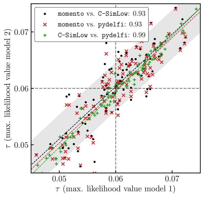
As well as investigating the average behaviour of the likelihoods, we have also compared them realisation by realisation. Fig. 7 shows scatter plots of the maximum likelihood values for each pair of likelihoods for SRoll2 with an input $\tau$ of $0.06$. To guide the eye, the grey shaded area shows the range expected for a $\pm 1\sigma$ error of $\delta\tau=0.006$. There is a high degree of correlation between all three likelihoods, especially between C-SimLow and pydelfi, as discussed in Sec. 4.3. This behaviour is expected since the pydelfi approach is effectively a generalisation of the simulation-based likelihood C-SimLow (fitting a set of Gaussian’s to the conditional distributions, instead of using a pre-defined functional form). The scatter between C-SimLow and pydelfi is about a sixth of a sigma, and between either C-SimLow or pydelfi and momento it is roughly half a sigma. Applied to the same simulations, methodological differences in the likelihood implementation lead to differences in the maximum likelihood value of $\tau$ of less than a standard deviation.

Table 2 also gives results for simulations in which the CMB realisations are generated from models with both lower ($0.05$) and higher ($0.07)$ values of $\tau$ than the fiducial value $\tau=0.06$ used to compute the QCS estimates. No bias is seen for any of the likelihoods confirming that the methods are insensitive to the choice of fiducial cosmology.

We note that the posteriors on $\tau$ determined from momento are about $10$% tighter than those determined from either C-SimLow or pydelfi. The distribution of peak maximum likelihood values of $\tau$, shown in Fig. 6, is also tighter for momento. We have therefore chosen to use momento as our default low-$\ell$ likelihood in Sec. 6 when combining with the high-$\ell$ $TTTEEE$ likelihood. Finally, all methods give average posterior widths that are slightly less than the scatter of their maximum likelihood values. The distribution of maximum likelihood values of $\tau$ should be closely related to the width of the posterior distribution but is not guaranteed to be the same. The agreement is, however, close enough to demonstrate that the widths of the posterior distributions are not seriously in error.

6 Results

In this section, we use the three likelihoods described in Sec. 4 to derive constraints on $\tau$ from both the Planck 2018 legacy maps (SRoll1) and the SRoll2 maps. In Sec. 6.1 we present results for the cross-correlation of the $100$ GHz and $143$ GHz full-mission maps, since this choice of maps was used in PCP18 and Pagano et al. (2020) to derive the results quoted in Eqs. (3a) and (3b). Sec. 6.2 presents a more extensive investigation of the SRoll2 data set comparing all six combinations of $100$ GHz and $143$ GHz detector set maps to test whether the results are sensitive to different splits of the Planck data. To reduce the computational burden, in Secs. 6.1 and 6.2 we perform one-dimensional parameter scans in $\tau$, allowing $A_{s}$ to change according to a fixed value of $10^{9}A_{s}e^{-2\tau}=1.870$. The other parameters of the base $\Lambda$CDM cosmology fixed to $H_{0}=67.04$, $\Omega_{\rm b}h^{2}=0.0221$, $\Omega_{\rm c}h^{2}=0.12$, $\Omega_{\nu}h^{2}=0.00064$, $\theta_{*}=1.0411$, $n_{\rm s}=0.96$ (PCP18). In Sec. 6.3, we relax the constraint on $10^{9}A_{s}e^{-2\tau}$ and perform a full Monte Carlo exploration of the six cosmological parameter space using momento in conjunction with the high-$\ell$ CamSpec v12.5HM likelihood (EG19).

6.1 Constraints using 100 $\times$ 143 full-mission QCS

Data Set	Likelihood	$\tau\ (EE)$	$\tau\ (TTTEEE)$
Planck 2018	C-SimLow	$0.0530\pm 0.0071$	…
	momento	$0.0507\pm 0.0063$	$0.0527\pm 0.0058$
	pydelfi	$0.0517\pm 0.0070$	$0.0513\pm 0.0078$
SRoll2	C-SimLow	$0.0582\pm 0.0057$	…
	momento	$0.0581\pm 0.0055$	$0.0604\pm 0.0052$
	pydelfi	$0.0588\pm 0.0054$	$0.0580\pm 0.0064$

Table 3: Summary of $\tau$ constraints for $100\times 143$ full-mission cross-spectra obtained using a simulation-based likelihood (C-SimLow), a likelihood approximation scheme (momento) and a density-estimation likelihood-free (pydelfi) approach. For $\tau(EE)$ we measure $\tau$ only using the low multipole polarisation data and for $\tau(TTTEEE)$ we compute a joint likelihood for temperature and polarisation data.

Figure 8: Summary plot of $\tau$ posteriors obtained from $100\times 143$ full-mission Planck 2018 and SRoll2 maps using a simulation-based likelihood (C-SimLow), a likelihood approximation scheme (momento) and a likelihood-free inference (pydelfi) approach. pydelfi and momento measure $\tau$ by, first, using only polarisation ($EE$) and, second, using temperature and polarisation data combined ($TTTEEE$). The vertical dashed lines and corresponding shaded regions indicate maximum likelihood values only using $EE$ polarisation data, for Planck 2018 (SRoll1) (PCP18) and SRoll2 (Pagano et al., 2020).

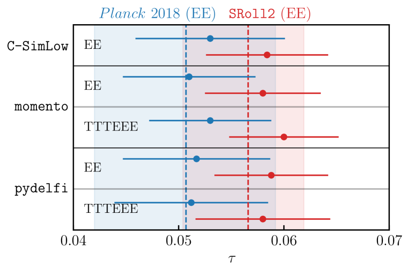
Table 3 summarises the results from foreground-cleaned $100\times 143$ full-mission maps. These results are plotted in Fig. 8 and compared with the results of Eqs. (3a) and (3b) (shown as the blue and red dashed lines respectively, together with $1\sigma$ errors shown by the red and blue shaded areas). For all three likelihood approximations, our results reproduce the upward movement in $\tau$ between SRoll1 and SRoll2 (as noted in Delouis et al. (2019)). Furthermore, the results from all three likelihoods are consistent with each other. There are, however, some interesting features that are worth noting:

$\ \ \nu\times\nu^{\prime}$	SRoll2	C-SimLow $($EE$){}^{*}$	C-SimLow ($EE$)	momento ($EE$)	momento ($TTTEEE$)	pydelfi ($EE$)	pydelfi ($TTTEEE$)∗
$\left[\mathrm{GHz^{2}}\right]$		∗no synch. removal					∗with compression
100 $\times$ 143	full $\times$ full	$0.0585\pm 0.0057$	$0.0582\pm 0.0057$	$0.0581\pm 0.0055$	$0.0604\pm 0.0052$	$0.0588\pm 0.0054$	$0.0580\pm 0.0064$
100 $\times$ 143	ds1 $\times$ ds1	$0.0642\pm 0.0077$	$0.0609\pm 0.0076$	$0.0595\pm 0.0068$	$0.0606\pm 0.0066$	$0.0594\pm 0.0074$	$0.0603\pm 0.0079$
	ds1 $\times$ ds2	$0.0622\pm 0.0073$	$0.0589\pm 0.0073$	$0.0586\pm 0.0067$	$0.0603\pm 0.0065$	$0.0607\pm 0.0072$	$0.0604\pm 0.0076$
	ds2 $\times$ ds1	$0.0559\pm 0.0071$	$0.0538\pm 0.0070$	$0.0579\pm 0.0067$	$0.0589\pm 0.0062$	$0.0531\pm 0.0066$	$0.0526\pm 0.0081$
	ds2 $\times$ ds2	$0.0597\pm 0.0066$	$0.0585\pm 0.0068$	$0.0570\pm 0.0066$	$0.0594\pm 0.0061$	$0.0579\pm 0.0065$	$0.0575\pm 0.0075$
100 $\times$ 100	ds1 $\times$ ds2	$0.0719\pm 0.0079$	$0.0643\pm 0.0079$	$0.0638\pm 0.0072$	$0.0657\pm 0.0071$	$0.0619\pm 0.0077$	$0.0662\pm 0.0076$
143 $\times$ 143	ds1 $\times$ ds2	$0.0702\pm 0.0082$	$0.0651\pm 0.0073$	$0.0676\pm 0.0068$	$0.0725\pm 0.0067$	$0.0656\pm 0.0075$	$0.0703\pm 0.0071$
mean	…	$0.0640\pm 0.0075$	$0.0603\pm 0.0074$	$0.0607\pm 0.0068$	$0.0629\pm 0.0065$	$0.0600\pm 0.0072$	$0.0612\pm 0.0076$

Table 4: Summary of $\tau$ posteriors derived from SRoll2 maps. Synchrotron and dust emission have been removed from the maps through template fitting, except for the column indicated which shows results obtained when only dust was subtracted. Hence the two C-SimLow columns illustrate the difference at the parameters level caused by the removal of synchrotron emission at the map level. The bottom row assumes that the six detector based likelihoods are highly correlated and shows the mean of these results. The pydelfi ($TTTEEE$) likelihood score compresses the power spectra before inferring the optical depth which results in wider posteriors than for the uncompressed pydelfi ($EE$)-only likelihood.

(i) The $TTTEEE$ pydelfi results have larger error bars than the $EE$ results alone, even though additional data is included in the $TTTEEE$ likelihood (though the best-fit value of $\tau$ hardly changes). As outlined in Sec. 4.3 one of the drawbacks of likelihood-free inference is that higher dimensional problems ($D\lower 2.15277pt\hbox{$\;\buildrel>\over{\sim}\;$}30$) require additional data compression. In our $TTTEEE$ implementation we compressed the $84$ power spectrum components for $2\leq\ell\leq 29$ into three summary statistics, one each for $TT$, $TE$ and $EE$, whereas for the $EE$-only implementation we were able to avoid compression entirely, using all 29 $EE$ power spectrum multipoles. The larger $TTTEEE$ pydelfi error is a consequence of lossy compression which actually degrades the $EE$ block. In fact, we found that a score-compressed $EE$ posterior from pydelfi gives a maximum likelihood value for $\tau$ that is lower by $\sim 0.25\sigma$ compared to the results without compression. With compression the $TE$ data does actually pull the posterior upwards by $\sim 0.3\sigma$, largely cancelling the effects of compression on $EE$. This is discussed further in App. C.3.

(ii) For momento, adding $TT$ and $TE$ spectra to $EE$ causes upward shifts in $\tau$ of approximately $0.002$ ($\sim 0.4\sigma$) for both SRoll1 and SRoll2 $\tau$ values. The posterior width is reduced by a modest $\sim 5\%$. This behaviour is consistent with the parameter-shift criteria developed by Gratton & Challinor (2020).

(iii) The SRoll2 likelihoods consistently yield higher values of $\tau$, and with slightly tighter errors, than the corresponding SRoll1 likelihoods.

(iv) The errors on $\tau$ from our application of C-SimLow to SRoll1 are about $20\%$ smaller than those quoted in Eqs. (3a). There are two reasons for this: (a) the results of PCP18 used a sub-optimal noise model based on Planck FFP8 end-to-end simulations for the QCS computations; (b) we subtracted a smoothed noise template at the map level (see Eq. (30)), which reduces the size of the posterior widths by $\sim 5$–$10\%$ for SRoll1, as explained in more detail in App. B.

Recently, a new set of Planck maps for the LFI and HFI frequency bands have been developed (Planck Collaboration, 2020e, hereafter NPIPE). As with SRoll1 and SRoll2, a set of systematic templates are fitted as part of the map-making stage. However, amongst other differences, NPIPE retains the CMB Solar dipole in each map and uses foreground polarisation priors at $30$, $217$ and $353$ GHz to break parameter degeneracies. The use of polarisation priors leads to a suppression of the polarisation signal at low multipoles, necessitating the calibration of $EE$ power spectrum transfer functions from end-to-end numerical simulations. The transfer functions corrections are quite large for the $EE$ multipoles $\ell=2$-$7$ that contain most of the information on $\tau$. The analysis of the NPIPE $100\times 143$ $EE$ spectrum presented in Planck Collaboration (2020e) gives a value for $\tau$ that is lower by $1.2\sigma-1.6\sigma$ compared to the results of Table 3. The $\tau$ results from NPIPE are therefore broadly in agreement with those from SRoll1 and SRoll2.

6.2 The optical depth from inter- and intra-frequency detector set combinations of SRoll2 maps

To assess the robustness of the results of the previous section, we have analysed the inter- and intra-frequency spectra computed from SRoll2 detector set maps. The SRoll2 cross-spectra used in this sub-section are shown in Fig. 5.

We stress that the likelihoods for each map pair have been computed/trained afresh using the appropriate detector set noise covariance matrices constructed from the relevant simulations. The results of the cross-checks, for each of the three likelihoods, are presented in Table 4. Each column lists the mean value for $\tau$ and the associated posterior width for the indicated spectrum combination.

Focusing on the results from momento, the posterior widths for $143$ds1$\times 143$ds2 are about $5\%$ smaller than for $100$ds1$\times 100$ds2, which is expected because the $143$ GHz maps are less noisy than the $100$ GHz maps. (The reduction in errors is, however, smaller in the other two likelihoods). More significantly, at multipoles $\ell=3-5$ the $143$ds1$\times 143$ds2 $EE$ spectrum lies above the $\tau=0.055$ theoretical line. As a consequence, for all likelihoods, the $143$ds1$\times 143$ds2 value of $\tau$ is higher than that for the $100\times 143$ spectra by about $1.4-2\sigma$. The $100$ds1$\times 100$ds2 also shows a preference for higher values of $\tau$ compared to the $100\times 143$ spectra, but to a lesser extent. This is suggestive of correlated residual systematics in the $100$ GHz detset and $143$ GHz detset maps which partially cancel when $100$ GHz detset maps are cross-correlated against $143$ GHz detset maps (as discussed by Pagano et al., 2020). The effects are relatively small, but in agreement with the conclusions of Pagano et al. (2020), our results suggest that the $100\times 143$ spectra are likely to provide the most reliable constraints on $\tau$.

The last row in Table 4 shows the mean of $\tau$ values for all of the inter- and intra-frequency cross detector set spectra constraints (ignoring correlations). The $100$ds1$\times 100$ds2 and $143$ds1$\times 143$ds2 results pull the means to slightly higher values of $\tau$ compared to the $100\times 143$ full-mission results, but only by about $0.5\sigma$. Thus, while there is some evidence of small systematic-related biases in the $100$ds1$\times 100$ds2 and $143$ds1$\times 143$ds2 $\tau$ values, the net effect of residual systematics on the $100\times 143$ full-mission results are probably at the level of a standard deviation or less. This statement depends on the fidelity of the noise and systematics simulations.

Columns 3 and 4 of Table 4 illustrate the impact of polarised synchrotron cleaning on $\tau$. (This test was done only for the C-SimLow likelihood). As expected, the effect on $\tau$ is most pronounced for $100$ds1$\times 100$ds2, with synchrotron cleaning lowering $\tau$ by about $1\sigma$ and bringing it into closer agreement with the $100\times 143$ full-mission result. However, the effects of synchrotron cleaning on the $100\times 143$ and $143$ds1$\times 143$ds2 spectra are significantly smaller, leading to changes in $\tau$ of $\sim 0.3\sigma$. Synchrotron cleaning, while non-negligible, is not a critical factor in the $\tau$ constraints from the $100\times 143$ spectra.

6.3 Full Monte Carlo Markov Chain Parameter Exploration

Likelihoods	CamSpec ($TTTEEE$) + Planck low-$\ell$ $TT$+ momento ($EE$)	CamSpec ($TTTEEE$) $+$ momento ($TTTEEE$)
	SRoll1
$\tau$	$0.0520^{+0.0055}_{-0.0062}$	$0.0552^{+0.0056}_{-0.0065}$
$\Omega_{b}h^{2}$	$0.02226\pm 0.00014$	$0.02228\pm 0.00015$
$\Omega_{c}h^{2}$	$0.1196\pm 0.0013$	$0.1194\pm 0.0013$
$100\theta_{\rm MC}$	$1.04103\pm 0.00028$	$1.04108\pm 0.00028$
$10^{9}A_{\mathrm{s}}e^{-2\tau}$	$1.880\pm 0.011$	$1.879\pm 0.012$
$n_{\rm s}$	$0.9669\pm 0.0043$	$0.9677\pm 0.0044$
$H_{0}$	$67.43\pm 0.55$	$67.57^{+0.54}_{-0.60}$
$\sigma_{8}$	$0.8086\pm 0.0066$	$0.8101\pm 0.0066$
$z_{\rm re}$	$7.45\pm 0.62$	$7.77\pm 0.61$
	SRoll2
$\tau$	$0.0592^{+0.0051}_{-0.0058}$	$0.0627^{+0.0050}_{-0.0058}$
$\Omega_{b}h^{2}$	$0.02229\pm 0.00015$	$0.02231\pm 0.00014$
$\Omega_{c}h^{2}$	$0.1194\pm 0.0013$	$0.1191\pm 0.0013$
$100\theta_{\rm MC}$	$1.04107\pm 0.00028$	$1.04109\pm 0.00027$
$10^{9}A_{\mathrm{s}}e^{-2\tau}$	$1.879\pm 0.011$	$1.878\pm 0.011$
$n_{\rm s}$	$0.9678\pm 0.0044$	$0.9688\pm 0.0047$
$H_{0}$	$67.56\pm 0.57$	$67.67\pm 0.57$
$\sigma_{8}$	$0.8136\pm 0.0063$	$0.8155\pm 0.0062$
$z_{\rm re}$	$8.18\pm 0.54$	$8.51\pm 0.52$

Table 5: Cosmological parameter constraints for $\Lambda$CDM cosmology obtained using momento with $100\times 143$ full-mission spectra at low-$\ell$ and the CamSpec v12.5HM ($TTTEEE$) at high-$\ell$ with 68% confidence levels. We compare the effect on the parameter constraints by combining our polarisation-only or joint temperature-polarisation low-$\ell$ likelihood momento with the high-$\ell$ ($\ell\geq 30$) likelihood CamSpec. The redshift of reionization $z_{\rm re}$ is defined in the same way as in PCP18.

We explore the full $\Lambda$CDM cosmological parameter space by combining our full-mission $100\times 143$ momento $EE$ and $TTTEEE$ likelihoods at low multipoles for both SRoll1 and SRoll2 with the high-$\ell$ CamSpec v12.5HM ($TTTEEE$) likelihood (which uses SRoll1 maps). The $EE$ momento likelihood uses the multipole range $2\leq\ell\leq 29$ and is utilised with the Planck 2018 low-$\ell$ $TT$ likelihood over the same multipole range. The momento $TTTEEE$ likelihood uses the multipole range $2\leq\ell\leq 10$ to speed up the low multipole likelihood evaluations. The multipoles $11-29$ in $TE$ and $EE$ have very little constraining power on $\tau$ and so little information on $\tau$ is lost by truncating the momento likelihood at $\ell=10$. The momento $TTTEEE$ likelihood is used with the Planck 2018 low-$\ell$ $TT$ likelihood over the multipole range $11\leq\ell\leq 29$, so that there are no multipole gaps in the $TT$ likelihood.

Table 5 lists the results of full MCMC exploration of the parameters of the base $\Lambda$CDM cosmology. These results are similar to those summarised in Table 3 for the one-dimensional $\tau$ scans. The SRoll2 results for $\tau$ are about $1\sigma$ higher than those from SRoll1, and the $TTTEEE$ momento likelihoods give values for $\tau$ that are about $0.3\sigma$ higher than those using the $EE$ momento likelihoods. The values for $10^{9}A_{s}e^{-2\tau}$ are also within about $1\sigma$ of the value assumed for the one-dimensional $\tau$ scans.

We can compare the results from momento with those of full parameter analyses using the SimBaL $EE$ likelihood combined with the low multipole $TT$ likelihood and the Plik high multipole $TTTEEE$ likelihood reported in PCP18 and Pagano et al. (2020):

$$\tau=0.0544^{+0.0070}_{-0.0081},\qquad\texttt{SRoll1},$$ (56a)

$$\tau=0.0591^{+0.0054}_{-0.0068},\qquad\texttt{SRoll2}.$$ (56b)

Our results using momento are higher by about $0.3-0.5\sigma$ and (formally) have slightly smaller error bars.

Figure 9: Parameter constraints for the base $\Lambda$CDM cosmology for $\tau$ and $\ln(10^{10}A_{s})$. The high-$\ell$ likelihood is CamSpec v12.5HM ($TTTEEE$) and the three different low-$\ell$ likelihood combinations are: (i) Planck $TT$ together with Planck $EE$ (grey), (ii) Planck $TT$ together with momento ($EE$) (red) and (iii) momento ($TTTEEE$) with Planck $TT$ (restricted to $11\leq\ell\leq 29$) (blue).

Figure 10: Marginalised posterior distributions for $\tau$ derived from the high-$\ell$ CamSpec v12.5HM ($TTTEEE$) likelihood combined with low-$\ell$ likelihoods as discussed in the text. The black lines in both plots use the low-$\ell$ Planck 2018 SimLow polarisation likelihood as in PCP18. The results of replacing SimLow with SRoll1 and SRoll2 momento likelihoods are shown in the left and right hand plots, respectively.

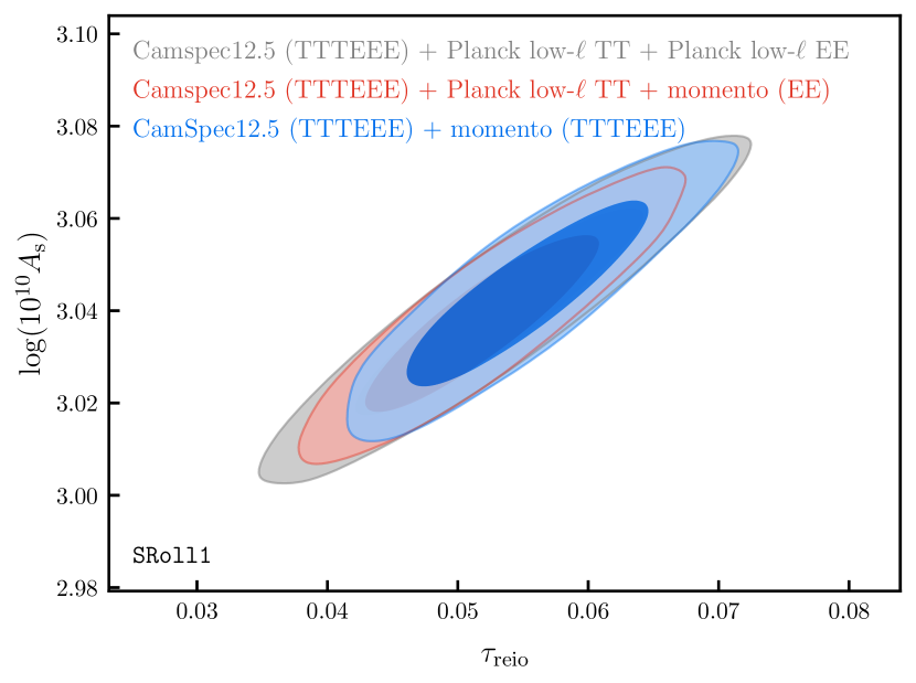
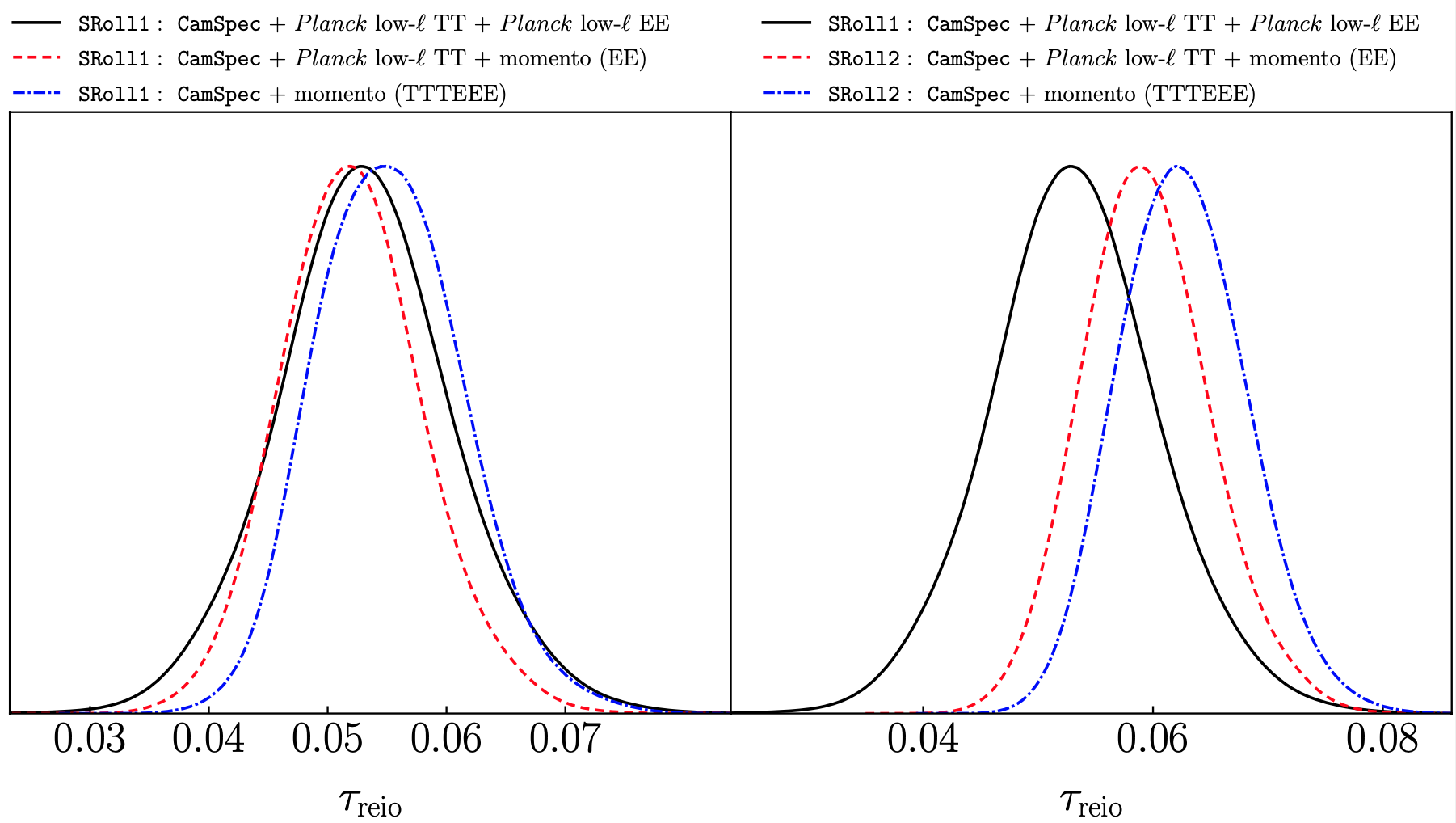
Fig. 9 illustrates the changes to the $\tau$ constraints caused by switching from SimLow to momento $EE$ and then to momento $TTTEEE$. This figure shows contours in the $\ln 10^{10}A_{s}$–$\tau$ plane for base $\Lambda$CDM. In each case we use the same high-$\ell$ CamSpec v12.5HM $TTTEEE$ likelihood for $30\leq\ell\leq 2500$ and so only the low-$\ell$ likelihoods change: grey contours for SimLow, red contours for SRoll1 momento $EE$ and blue for SRoll1 momento $TTTEEE$. Interestingly, the momento $TTTEEE$ likelihood disfavours values of $\tau\lower 2.15277pt\hbox{$\;\buildrel<\over{\sim}\;$}0.04$ that are already excluded by the Gunn-Peterson test (see Eq. (2)). In other words, the posteriors of the momento likelihood are consistent with what we know about the intergalactic medium.

The main results of this section are summarised in Fig. 10. The plot to the left shows the marginalised posterior distribution for $\tau$ for CamSpec combined with the SRoll1 likelihoods as described above. This shows the small shifts in $\tau$ when we use the SRoll1 momento likelihoods in place of the Planck 2018 low-$\ell$ $EE$ likelihood. The right hand plot shows how the posteriors change if we use the SRoll2 momento likelihoods. The momento constraints shift to higher values of $\tau$ as a consequence of the changes to the HFI map-making. We take as our ‘best’ estimate of $\tau$ and redshift of reionization, $z_{\rm re}$, the results from the combined CamSpec + SRoll2 momento $TTTEEE$ likelihood:

$$\tau=0.0627^{+0.0050}_{-0.0058},\qquad z_{\rm re}=8.51\pm 0.52,$$ (57)

slightly higher than the result of Eq. (56b).

7 Summary and conclusions

The determination of the optical depth to reionization $\tau$ from the CMB is extremely challenging, yet of great importance for our understanding of the intergalactic medium and the formation of the first stars and galaxies. Improvements in the HFI map-making algorithms described in PSRoll1 and PSRoll2 have led to maps which have low levels of residual systematics in polarisation resulting in low values of $\tau$ (Eqs. (56a) and (56b)). Producing high fidelity polarisation maps is only one part of the story however. To derive accurate constraints on $\tau$ requires an accurate likelihood. The construction of a $TTTEEE$ likelihood is not straightforward at low multipoles for maps with complex noise properties and partial sky coverage. There is no analytic guide to help create such a likelihood, particularly if the likelihood is built around quadratic cross-spectra. In PSRoll1 and PSRoll2, an $EE$ likelihood was constructed based on a relatively small number of end-to-end simulations, leading to the results of Eqs. (56a) and (56b).

In this paper we have developed and compared three likelihood techniques on the Planck SRoll1 and SRoll2 maps. The first is a variant of the SimBaL scheme described in PSRoll1 and PSRoll2, but using more accurate simulation-based noise covariance matrices to construct quadratic cross-spectra and to generate a large number of independent noise realisations. The second (momento) is based on the glass maximum entropy approach developed by Gratton (2017) and the third (pydelfi) is a density-estimation ‘likelihood free’ scheme that follows closely the implementation described by Alsing et al. (2019). The momento and pydelfi approaches can be generalised to construct low multipole $TTTEEE$ likelihoods. (Though not explored in this paper, it is straightforward to adapt these schemes to develop likelihoods incorporating other low multipole spectra, e.g. $BB$, $ET$.)

Our main conclusion is that all three likelihood methods are in good agreement and support the conclusions on $\tau$ reported in PCP18 and Pagano et al. (2020); we do, however, see small differences between the likelihoods as summarised in Tables 3 and 4. Using only the spectra at low multipoles, our results tend to give higher values of $\tau$ than those using SimBaL (Eqs. (3a)) and (3b)) by up to $\sim 0.8\sigma$. However, if we include the high multipole CamSpec $TTTEEE$ likelihood, the results for $\tau$ using the SRoll2 momento $EE$ likelihood is very close to that given in Eq. (56b) though with a smaller formal error.

We constructed low multipole $TTTEEE$ likelihoods using momento and pydelfi. For momento, using a $TTTEEE$ likelihood leads to smaller errors on $\tau$ than using $EE$ alone, as expected. However, we had to apply data compression to produce a pydelfi $TTTEEE$ likelihood that was numerically fast and robust enough for likelihood analysis. This resulted in a loss of information and to $\tau$ constraints that had slightly larger errors using pydelfi $TTTEEE$ compared to using pydelfi $EE$, though with no evidence of any bias; see App. C.3 for a detailed discussion.

We also made a thorough analysis of different detector set data splits at $100$ and $143$ GHz, as summarised in Table 4. For all likelihoods, the $100$ds1$\times 100$ds2 and $143$ds1$\times 143$ds2 spectra give $\tau$ values that are higher than those from the baseline $100\times 143$ full-mission analysis by between $0.8$ and $2\sigma$. There is therefore evidence that within a frequency band there remain correlated systematic effects (as is apparent visually from Fig. 3) that bias $\tau$ high by $\sim 0.01$. The series of null tests described in PSRoll2, together with the absence of any statistically significant $B$-mode signal at low multipoles, suggests that the $100\times 143$ full-mission cross-spectra should provide unbiased estimates of $\tau$. The changes between PSRoll1 and PSRoll2 suggest an upper bound of about $1\sigma$ to biases in $\tau$ caused by residual systematics.

As noted above, the likelihood techniques explored here have wider applications and can be adapted to other problems involving low multipole polarisation maps, particularly if the maps have complex noise properties. An obvious example is the measurement of the tensor-to-scalar ratio $r$, in addition to $\tau$, from the forthcoming CMB satellite LiteBIRD (Sugai et al., 2020).

Data availability

The data underlying this article will be shared on reasonable request. The Planck 2018 (SRoll1) and SRoll2 frequency maps and end-to-end simulations are publicly available: SRoll1 simulations (labelled FFP10) at https://pla.esac.esa.int; SRoll2 simulations at http://sroll20.ias.u-psud.fr.

Appendix A Analytic solution to the noise inference problem

In order to minimise Eq. (28) analytically for $\mathbf{\Psi}$, we first consider the variation in $\delta\mathcal{S}$ caused by small changes in $\mathbf{M}$. Omitting the $n_{s}/2$ prefactor, we have:

$$\delta\mathcal{S} =\ \mathrm{tr}(\delta(\mathbf{M}^{\raisebox{0.60275pt}{$\scriptscriptstyle-1$}})\,\hat{\mathbf{N}})+\delta\ln|\mathbf{M}|$$ (58)

$$=\ \mathrm{tr}\left[-\mathbf{M}^{\raisebox{0.60275pt}{$\scriptscriptstyle-1$}}(\delta\mathbf{M})\mathbf{M}^{\raisebox{0.60275pt}{$\scriptscriptstyle-1$}}\hat{\mathbf{N}}+\mathbf{M}^{\raisebox{0.60275pt}{$\scriptscriptstyle-1$}}(\delta\mathbf{M})\right]$$ (59)

$$=\ \mathrm{tr}\left[-\mathbf{M}^{\raisebox{0.60275pt}{$\scriptscriptstyle-1$}}\mathbf{Y}(\delta\mathbf{\Psi})\mathbf{Y}^{\top}\mathbf{M}^{\raisebox{0.60275pt}{$\scriptscriptstyle-1$}}\hat{\mathbf{N}}+\mathbf{M}^{\raisebox{0.60275pt}{$\scriptscriptstyle-1$}}\mathbf{Y}(\delta\mathbf{\Psi})\mathbf{Y}^{\top}\right]$$ (60)

using the standard results for matrices that $\delta(\mathbf{M}^{\raisebox{0.60275pt}{$\scriptscriptstyle-1$}})=-\mathbf{M}^{\raisebox{0.60275pt}{$\scriptscriptstyle-1$}}(\delta\mathbf{M})\mathbf{M}^{\raisebox{0.60275pt}{$\scriptscriptstyle-1$}}$ and $\delta\ln|\mathbf{M}|=\ \mathrm{tr}\mathbf{M}^{\raisebox{0.60275pt}{$\scriptscriptstyle-1$}}\delta\mathbf{M}$, and $\delta\mathbf{M}=\mathbf{Y}\delta\mathbf{\Psi}\mathbf{Y}^{\top}$. Next we use the cyclic property of the trace to obtain:

$$\delta\mathcal{S} =\ \mathrm{tr}\left[\delta\mathbf{\Psi}\left(\mathbf{Y}^{\top}\mathbf{M}^{\raisebox{0.60275pt}{$\scriptscriptstyle-1$}}(\mathbf{M}-\hat{\mathbf{N}})\mathbf{M}^{\raisebox{0.60275pt}{$\scriptscriptstyle-1$}}\mathbf{Y}\right)\right].$$ (61)

At the minimum we require $\delta\mathcal{S}=0$ for arbitrary $\delta\Psi$ and thus need

$$\mathbf{Y}^{\top}\mathbf{M}^{\raisebox{0.60275pt}{$\scriptscriptstyle-1$}}(\mathbf{M}-\hat{\mathbf{N}})\mathbf{M}^{\raisebox{0.60275pt}{$\scriptscriptstyle-1$}}\mathbf{Y}=\mathbf{0}.$$ (62)

We now use the generalised Sherman–Morrison–Woodbury formula

$$\mathbf{M}^{\raisebox{0.60275pt}{$\scriptscriptstyle-1$}}=\mathbf{N}^{\raisebox{0.60275pt}{$\scriptscriptstyle-1$}}-\mathbf{N}^{\raisebox{0.60275pt}{$\scriptscriptstyle-1$}}\mathbf{Y}(\mathbf{\Psi}^{\raisebox{0.60275pt}{$\scriptscriptstyle-1$}}+\mathbf{Y}^{\top}\mathbf{N}^{\raisebox{0.60275pt}{$\scriptscriptstyle-1$}}\mathbf{Y})^{\raisebox{0.60275pt}{$\scriptscriptstyle-1$}}\mathbf{Y}^{\top}\mathbf{N}^{\raisebox{0.60275pt}{$\scriptscriptstyle-1$}}$$ (63)

(and adding and subtracting $\mathbf{\Psi}^{\raisebox{0.60275pt}{$\scriptscriptstyle-1$}}$) to rewrite $\mathbf{Y}^{\top}\mathbf{M}^{\raisebox{0.60275pt}{$\scriptscriptstyle-1$}}$ as

$$\mathbf{Y}^{\top}\mathbf{M}^{\raisebox{0.60275pt}{$\scriptscriptstyle-1$}} =\mathbf{Y}^{\top}\left(\mathbf{N}^{\raisebox{0.60275pt}{$\scriptscriptstyle-1$}}-\mathbf{N}^{\raisebox{0.60275pt}{$\scriptscriptstyle-1$}}\mathbf{Y}(\mathbf{\Psi}^{\raisebox{0.60275pt}{$\scriptscriptstyle-1$}}+\mathbf{Y}^{\top}\mathbf{N}^{\raisebox{0.60275pt}{$\scriptscriptstyle-1$}}\mathbf{Y})^{\raisebox{0.60275pt}{$\scriptscriptstyle-1$}}\mathbf{Y}^{\top}\mathbf{N}^{\raisebox{0.60275pt}{$\scriptscriptstyle-1$}}\right)$$ (64)

$$=\mathbf{Y}^{\top}\mathbf{N}^{\raisebox{0.60275pt}{$\scriptscriptstyle-1$}}-(\mathbf{Y}^{\top}\mathbf{N}^{\raisebox{0.60275pt}{$\scriptscriptstyle-1$}}\mathbf{Y}+\mathbf{\Psi}^{\raisebox{0.60275pt}{$\scriptscriptstyle-1$}}-\mathbf{\Psi}^{\raisebox{0.60275pt}{$\scriptscriptstyle-1$}})$$

$$\qquad\qquad\times(\mathbf{\Psi}^{\raisebox{0.60275pt}{$\scriptscriptstyle-1$}}+\mathbf{Y}^{\top}\mathbf{N}^{\raisebox{0.60275pt}{$\scriptscriptstyle-1$}}\mathbf{Y})^{\raisebox{0.60275pt}{$\scriptscriptstyle-1$}}\mathbf{Y}^{\top}\mathbf{N}^{\raisebox{0.60275pt}{$\scriptscriptstyle-1$}}$$ (65)

$$=\mathbf{\Psi}^{\raisebox{0.60275pt}{$\scriptscriptstyle-1$}}(\mathbf{\Psi}^{\raisebox{0.60275pt}{$\scriptscriptstyle-1$}}+\mathbf{Y}^{\top}\mathbf{N}^{\raisebox{0.60275pt}{$\scriptscriptstyle-1$}}\mathbf{Y})^{\raisebox{0.60275pt}{$\scriptscriptstyle-1$}}\mathbf{Y}^{\top}\mathbf{N}^{\raisebox{0.60275pt}{$\scriptscriptstyle-1$}}\ .$$ (66)

Substituting this and its transpose into Eq. (62) yields

$$\mathbf{Y}^{\top}\mathbf{N}^{\raisebox{0.60275pt}{$\scriptscriptstyle-1$}}\left[\mathbf{N}+\mathbf{Y}\mathbf{\Psi}\mathbf{Y}^{\top}-\hat{\mathbf{N}}\right]\mathbf{N}^{\raisebox{0.60275pt}{$\scriptscriptstyle-1$}}\mathbf{Y}=\mathbf{0}.$$ (67)

Rearranging this for $\mathbf{\Psi}$ then gives the desired Eq. (29).

Appendix B Smoothed Template Subtraction

Figure 11: Effect of smoothed noise template subtraction on the $\tau$ posterior computed from $100\times 143$ full-mission cross-spectra of Planck 2018 maps. This test is performed using the simulation-based likelihood C-SimLow. The solid (dashed) line shows the posterior obtained when the subtraction is (is not) performed.

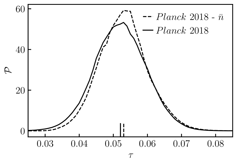
This appendix discusses the effect of smoothed template subtraction. The ADCNL effectively leads to CMB-independent offsets in Planck HFI maps. The CMB signal can then suffer chance correlations with these offsets, leading to additional scatter in power spectra. This effect is seen in simulations and, as discussed in Sec. 3.2, can potentially be mitigated by computing a smoothed estimate of the offset for each map and then subtracting the appropriate estimate from each of the QCS input maps. Applying this prescription to SRoll1 spectra leads to a $\sim 10\%$ reduction in the posterior width for $\tau$ from SRoll1 and to a $\sim 5\%$ reduction from SRoll2. This is consistent with the hypothesis that SRoll2 better reduces large-scale residuals than SRoll1 and so sees less of an improvement. Note that the procedure of removing smoothed templates from real data only leads one closer to the truth if the simulations from which the smoothed templates are computed are relatively accurate not only in the power spectrum domain but also in the map domain.

Fig. 11 shows the effect of smoothed template subtraction on the $\tau$ posterior for Planck 2018 data using C-SimLow ($EE$). The solid line yields a posterior of $\tau=0.0521\pm 0.0077$ where no smoothed templates have been subtracted. The dashed line yields a posterior $\tau=0.0530\pm 0.0071$.

B.1 Comparison between SRoll1 and SRoll2

Figure 12: QCS estimates for $TE$, $EE$ and $BB$ $100\times 143$ full-mission foreground-cleaned cross-spectra computed for the difference between SRoll2 and SRoll1 maps. The black points show the spectra computed before any smoothed templates are removed, while the red points show the spectra computed after the maps have their corresponding templates subtracted. The error bars for the cross-spectra are taken from the $BB$ spectrum as the signal has been removed. The $TT$ residual spectrum is not shown as it is consistent with zero. Note that the $BB$ errors plotted on the $TE$ spectrum are smaller than the points at low $\ell$; there are significant changes (relative to the $BB$ noise) between SRoll1 and SRoll2 in $TE$.

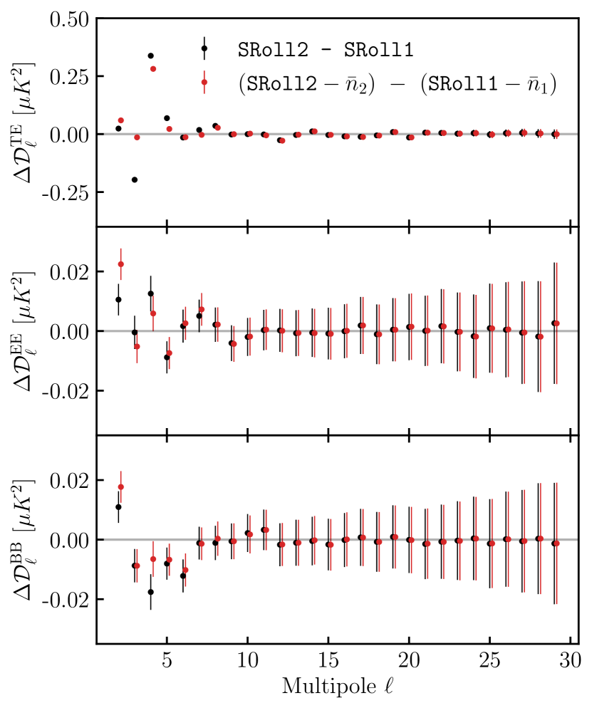
Power spectra of the difference maps computed between SRoll1 and SRoll2 are shown in Fig. 12. The error bars are based on the error estimates obtained from the $BB$ spectra since no signal should be left in the difference maps. Both maps have been foreground cleaned with the respective maps, as detailed in Sec. 3.1. The red points show the spectra computed from maps that have corresponding smoothed templates (denoted $n_{1}$ for SRoll1 and $n_{2}$ for SRoll2) subtracted. The black points show the difference at the map level without subtracting the templates. We note that the subtractions only have large effects for $\ell\leq 4$ (as one would expect given that this is the maximum multipole retained in the templates) and, except for the quadrupole, reduce the residuals. With or without the template subtractions, the residual cross-spectra show differences for the very low multipoles below $\ell\sim 10$ for $TE$, $EE$ and $BB$. We do not show the $TT$ spectrum since it is signal dominated and, as shown in Fig. 4, the $TT$ spectra are almost identical for SRoll1 and SRoll2. This test confirms that the SRoll2 map-making algorithm indeed alters large-scale polarisation features relative to SRoll1.

Appendix C Technical details for density-estimation likelihood-free inference

In the present Appendix, we will elaborate on the technical details of the likelihood-free inference code pydelfi (Alsing et al., 2019), based on theoretical ground work by Leclercq (2018); Alsing et al. (2018); Alsing et al. (2019); Lueckmann et al. (2018); Papamakarios et al. (2018). These methods provide a means of performing Bayesian inference when it is possible to produce high accuracy simulations of the observables in question, even when it is not possible to write down an explicit analytic expression for the likelihood. Examples of such problems include measuring cosmological parameters from type Ia supernovae (Weyant et al., 2013), weak lensing peak counts (Lin & Kilbinger, 2015; Jeffrey et al., 2020), analysing the galaxy-halo connection (Hahn et al., 2017), inferring photometric redshifts and size evolution of galaxies (Carassou et al., 2017), measuring cosmological redshift distributions (Kacprzak et al., 2018), estimating the ionising background from the Lyman-$\alpha$ and Lyman-$\beta$ forests (Davies et al., 2018) and inferring the sum of the masses of Andromeda and the Milky Way (Lemos et al., 2021).

The key principle behind LF methods is the understanding that a simulated observable, $\mathbf{d}$, and the input parameters, $\bf{\theta}$, are a sample from the joint probability distribution $\mathcal{P}(\mathbf{d},\mathbf{\theta}|\mathcal{M})$ conditioned on the theoretical model. For compactness we will hereafter suppress the conditional aspect of the distribution and make the assumption that our simulations accurately represent the true physical process. With a sufficiently large number of samples from $\mathcal{P}(\mathbf{d},\mathbf{\theta})$ we can obtain a posterior on the parameters by selecting the samples that have $\mathbf{d}_{\mathrm{data}}=\mathbf{d}_{\mathrm{sim}}$. In many situations, it is essentially impossible to obtain $\mathbf{d}_{\mathrm{data}}\equiv\mathbf{d}_{\mathrm{sim}}$ and thus $|\mathbf{d}_{\mathrm{data}}-\mathbf{d}_{\mathrm{sim}}|<\epsilon$ is used (for some suitable metric).

An immediate challenge to the above idea is that, for many situations including cases in cosmology, it can require an incredibly large number of simulations to obtain samples from the posterior, especially if one requires a small $\epsilon$ parameter. This is particularly true when the dimension of the observable is large. This challenge can be addressed with density estimation likelihood-free inference (delfi). The conceptually simplest delfi methods use a density estimator to obtain a parametric form for the joint distribution $\mathcal{P}(\mathbf{d},\theta|w)$, where w are the parameters of the density estimator. These methods have been found to require many orders of magnitude fewer simulations. In this work we use a slight variation: we use a density estimator to model the conditional distribution $\mathcal{P}(\mathbf{d}|\theta,w)$, utilising the fact that, when conditioned on the parameters, $\mathbf{d}_{\rm sim}$ is a sample from $\mathcal{P}(\mathbf{d}|\theta)$. This variation means that one can be agnostic about the properties of the chosen simulation points; see Alsing et al. (2019) for a more detailed discussion. The likelihood is then obtained by evaluating this conditional distribution at the observed data $\mathbf{d}_{0}$. Given the likelihood and a prior, we then use MCMC sampling to obtain posterior samples.

C.1 Masked Autoregressive Flows

We require the density estimation to be flexible enough to allow us to accurately approximate the true conditional distribution and also to be computationally tractable in order to both fit and use. Recent work by e.g. Papamakarios & Murray (2016); Uria et al. (2016) have shown that Masked Autoregressive Flows (MAFs) provide one such method.

MAFs rely on two steps to achieve these goals. Firstly they utilise the chain rule to express the multidimensional conditional distribution, $\mathcal{P}(\mathbf{d}|\mathbf{\theta})$, as a series of one dimensional conditionals

$$\mathcal{P}(\mathbf{d}|\mathbf{\theta})=\prod_{i=1}^{n}\mathcal{P}(d_{i}|\mathbf{d}_{1:i-1},\mathbf{\theta})\ .$$ (68)

A model utilising this decomposition is known as an autoregressive model. Next, a form is chosen for the one dimensional conditional distributions. We assume the conditionals are one dimensional Gaussian distributions whose means, $\mathbf{\mu}$, and standard deviations, $\mathbf{\sigma}$, depend on $\mathbf{d}_{1:i-1}$ and $\mathbf{\theta}$. To achieve the desired flexibility we use neural networks, with parameters $\mathbf{w}$, to parametrise these functions as $\mathbf{\mu}(\mathbf{d}_{1:i-1},\mathbf{\theta}|\mathbf{w})$ and $\mathbf{\sigma}(\mathbf{d}_{1:i-1},\mathbf{\theta}|\mathbf{w})$. As was shown in Germain et al. (2015) this setup can equivalently be formulated as developing a mapping from $\mathbf{d}$ to the variable $u_{i}=x_{i}-\mu_{i}(\mathbf{d}_{1:i-1},\mathbf{\theta}|\mathbf{w})/\sigma_{i}(\mathbf{d}_{1:i-1},\mathbf{\theta}|\mathbf{w})$ where $\mathbf{u}$ are independent zero mean, unit variance Gaussian random variables. This means the density estimator has the simple form

$$\mathcal{P}(\mathbf{d}|\mathbf{\theta},\mathbf{w})=\mathcal{N}[\mathbf{u}(\mathbf{d,\theta;w})|\mathbf{0,1}]\times\prod_{i=1}^{n}\sigma_{i}^{n}(\mathbf{d,\theta;w}),$$ (69)

where the product over the standard deviations is the Jacobian from transforming from $\mathbf{u}$ to $\mathbf{d}$. We use an efficient implementation of this setup called the Gaussian Masked Autoencoders for Density Estimation and hereafter refer to this method as MADE.

There are two main limitations for using MADE: first, they depend sensitively on the order of factorisation and, second, the assumption of Gaussian conditionals may be overly restrictive. To mitigate these shortcomings we stack a series of MADEs to make a MAF. The output $\mathbf{u}$ of each MADE is the input of the next one. The conditional density estimator is thus given by

$$\mathcal{P}(\mathbf{d}|\mathbf{\theta;w}) =\prod_{i}\mathcal{P}(d_{i}|\mathbf{d}_{1:i-1},\mathbf{\theta})$$

$$=\mathcal{N}[\mathbf{u}(\mathbf{d,\theta;w})|\mathbf{0,1}]\times\prod_{n=1}^{N_{\rm MADE}}\prod_{i=1}^{n}\sigma_{i}^{n}(\mathbf{d,\theta;w})\ .$$ (70)

Thus we obtain a conditional distribution that is both analytically tractable (a simple product of Gaussians) and highly flexible.

Finally we fit the weights of the neural network as detailed in Sec. 4.3 around Eq. (54). By minimising the negative loss function in Eq. (55) we train the neural density estimators (NDEs) with respect to the network weights. The problem of overfitting is mitigated by applying the standard machine learning procedures of early stopping, dropouts and the random selection of training and testing subsets.

C.2 Architecture of pydelfi

No.	$N_{\rm MADE}$	Hidden Layers	Units	Validation Loss	$\tau$ Posterior
1	20	2	50	26.0	$0.0519\pm 0.0071$
2	10	2	50	25.9	$0.0512\pm 0.0071$
3	5	2	50	26.0	$0.0526\pm 0.0073$
4	3	2	75	26.0	$0.0526\pm 0.0069$
5	5	2	75	25.8	$0.0529\pm 0.0073$
6	10	2	75	25.9	$0.0514\pm 0.0070$
7	20	2	75	26.0	$0.0519\pm 0.0068$
8	5	3	35	26.0	$0.0521\pm 0.0067$

Table 6: Details of the eight MAFs making up the NDEs of the pydelfi architecture used in this paper, along with the $\tau$ posteriors from each NDE for the SRoll1 $100\times 143$ $EE$ analysis. (The individual posteriors are shown in Fig. 13.)

Figure 13: Planck 2018 posteriors obtained from our eight NDEs in our pydelfi architecture. The black lines show the individual constraints, and the blue solid line shows the weighted average that makes our pydelfi result. (The means and standard deviations of the individual posteriors are given in Table 6.)

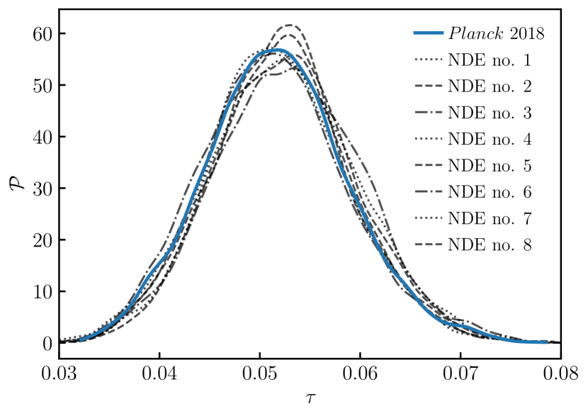
For the density estimation, we select an ensemble of NDEs, all of them MAFs, with different numbers of MADEs, hidden layers and neurons per layer, as shown in Table 6. All the NDEs use a $\tanh$ activation function, and are trained using the stochastic gradient optimiser adam (Kingma & Ba, 2014). To shorten training times of the NN, we trained the model on graphics processing units. To avoid overfitting, we use one tenth of the training set at each training cycle to validate our posterior (i.e. perform ‘early-stopping’) and use a learning rate of 0.001.

The result from density estimation of the different NDEs is shown in Fig. 13. This is a powerful cross-check to determine whether or not our architecture was chosen appropriately, remembering that there is no general procedure for choosing NN architectures. Each NDE yields a consistent posterior, also shown in Table 6. All the NDEs are then stacked and weighted by the loss evaluated during training,

$$\mathcal{P}(\bf{t}|\bf{\theta;w})=\sum_{\alpha=1}^{N_{\rm NDE}}\beta_{\alpha}p_{\alpha}(\bf{t}|\bf{\theta;w})\ ,$$ (71)

following (Alsing et al., 2019), also illustrated in Fig. 13. This is motivated by the demonstration of Smyth & Wolpert (1998, 1999) that stacking multiple NDEs is typically more robust than using an individual one. (In fact, the high degree of consistency between the NDEs makes us suspect that using fewer of them would still be sufficient to constrain $\tau$, saving training time.)

C.3 Score and data compression

To compute a joint likelihood using low multipole temperature and polarisation QCS spectra ($TT$, $TE$, $EE$) an additional compression step is required to reduce the dimensionality of the problem. Therefore, the full $N$-dimensional data set $\mathbf{D}\in\mathbb{R}^{N}$ is first compressed to quadratic cross-spectra, i.e. summary statistics $\mathbf{d}\in\mathbb{R}^{M}$, with $M<N$. Then, we score compress the vector of $M$ power spectrum measurements $\mathbf{d}$ into a vector of $n$ components $\mathbf{t}\in\mathbb{R}^{n}$, with $n<M<N$. In order to inform the choice of statistic for the score compression, an approximate form of the log-likelihood function $\mathcal{L}$ is assumed. The statistic $\mathbf{t}$ is then the gradient of the approximate log-likelihood, evaluated at some fiducial parameter values $\mathbf{\theta}_{*}$, i.e. $\mathbf{d}\mapsto\mathbf{t}=\nabla_{\mathbf{\theta}}\mathcal{L}_{*}$.

In the main body of the paper we compressed the $TT$, $TE$ and $EE$ cross-spectra separately for computational simplicity. This is suboptimal, as power spectrum elements between spectra are correlated. However this does not bias our cosmological constraints and pydelfi does capture residual correlations between the individual $TT$, $TE$ and $EE$ statistics. The approximate log-likelihood we use for the score compression step is the analytic result that can be derived for cross-spectra computed on the full sky with Gaussian isotropic noise, namely the variance-gamma distribution (Pearson et al., 1929):

$$\mathcal{P}(\hat{C}^{XY}_{\ell}) =\frac{(2\ell+1)\left|\hat{C}^{XY}_{\ell}\right|^{\ell}}{\Gamma(\frac{2\ell+1}{2})\sqrt{2^{2\ell}\pi(1-\rho_{\ell}^{2})\left(C_{\ell}^{XX}C_{\ell}^{YY}\right)^{\ell+1}}}$$

$$\quad\times K_{\ell}\left(\frac{(2\ell+1)\left|\hat{C}_{\ell}^{XY}\right|}{(1-\rho_{\ell}^{2})\sqrt{C_{\ell}^{XX}C_{\ell}^{YY}}}\right)$$

$$\quad\times\exp\left(\frac{(2\ell+1)\rho_{\ell}\left|\hat{C}_{\ell}^{XY}\right|}{(1-\rho_{\ell}^{2})\sqrt{C^{XX}_{\ell}C^{YY}_{\ell}}}\right)\ .$$ (72)

Here $\Gamma(n)$ is the gamma function, $K_{n}(x)$ is the modified Bessel function of the second kind and $\rho_{\ell}\equiv C^{XY}/\sqrt{C^{XX}C^{YY}}$ is the correlation coefficient. Using a fiducial model with $\tau=0.06$, we differentiate Eq. (C.3) to obtain

$$t=\left.\nabla_{\mathbf{\tau}}\ln\mathcal{P}(\hat{C}^{XY}_{\ell})\right|_{\theta_{*}},$$ (73)

one each for $TT$, $TE$ and $EE$.

We then fit the parameters of the pydelfi likelihood using the compressed statistics of the simulations and the compressed data vector, yielding the pair $\{\tau,t\}$. For the case where we only consider $EE$, the compressed statistic is related to the maximum likelihood estimate for $\tau$; see Alsing et al. (2018) for a more detailed discussion. The limitations of the compression steps are discussed further in Alsing et al. (2018).

C.4 Effect of score compression on the maximum likelihood value of $\tau$ and comparison between pydelfi and momento

Figure 14: Score-compressed pydelfi posteriors from SRoll2 $100\times 143$ spectra. The individual $\tau$ posteriors for the $EE$ (dashed black line), $TE$ (dash-dotted black line) and $TT$ (dotted black line) statistics are shown, along with the result from the three-statistic $TTTEEE$ likelihood (solid red line).

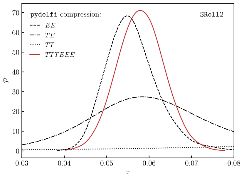
This section considers in more detail the properties of the score-compressed pydelfi likelihoods, both amongst themselves and then in comparison with momento.

First, in Fig. 14 we illustrate the score-compressed posteriors obtained with $100\times 143$ spectra from SRoll2 frequency maps using pydelfi. The different posteriors from the $EE$ (dashed line), $TE$ (dash-dotted line) and $TT$ (dotted line) statistics are shown, along with that from the combined three-statistic $TTTEEE$ likelihood (solid red line). These all used the full multipole range ($2\leq\ell\leq 29$) for the construction of the statistic(s). The $EE$ posterior is most constraining, the $TE$ posterior somewhat so, whereas the $TT$ one hardly varies over the $\tau$ scan. In the three-statistic likelihood, the addition of $TE$ information moves the mean $\tau$ value upwards by $\sim 0.25\sigma$ from that from the $EE$-statistic likelihood. This upwards shift is also seen for momento in Table 3 but is not apparent there for pydelfi. This is because the table shows results from the non-score-compressed pydelfi $EE$ likelihood and from the score-compressed three-statistic pydelfi $TTTEEE$ likelihood. The upwards shift from adding $TE$ partially cancels the downward movement caused in passing from a full $EE$ likelihood to a score-compressed one.

Figure 15: Comparison of $\tau$ posteriors from $100\times 143$ SRoll2 $TTTEEE$ spectra using pydelfi with (dotted line) and without compression (dashed line) and using momento (solid line). For this test all likelihoods use the same multipole range of $2\leq\ell\leq 10$. We note that avoiding score compression for pydelfi results in a shift upwards by $\sim 0.5\sigma$ of the $\tau$ maximum likelihood value compared to that from the score compressed likelihood, leading to a similar result to momento.

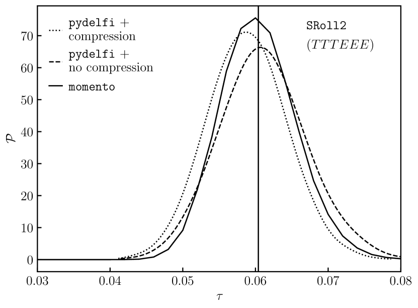
Second, to further understand how pydelfi performs in comparison to momento in the joint temperature-polarisation case, we produce a version of pydelfi that does not need score compression. By limiting the power spectrum multipoles to those that are most constraining for $\tau$, i.e. $2\leq\ell\leq 10$, rather than $2\leq\ell\leq 29$, we have a computationally-manageable 27-dimensional problem, rather than a difficult 84-dimensional one. Comparing the posteriors with and without score compression on SRoll2 maps for the three-statistic $TTTEEE$ likelihoods, we obtain:

$$\tau=0.0578\pm 0.0063,\quad({\rm\texttt{pydelfi},\,\ell\leq 10+comp.}),$$ (74a)

$$\tau=0.0612\pm 0.0060,\quad({\rm\texttt{pydelfi},\,\ell\leq 10+no\ comp.}).$$ (74b)

Fig. 15 illustrates these posteriors and compares them to the momento posterior. This confirms the role of the score compression discussed above in affecting constraints on $\tau$.

References

- Aiola et al. (2020) Aiola S., et al., 2020, J. Cosmology Astropart. Phys., 2020, 047
- Alsing et al. (2018) Alsing J., Wandelt B., Feeney S., 2018, MNRAS, 477, 2874
- Alsing et al. (2019) Alsing J., Charnock T., Feeney S., Wandelt B., 2019, MNRAS, 488, 4440
- Bautista et al. (2020) Bautista J. E., et al., 2020, MNRAS,
- Carassou et al. (2017) Carassou S., de Lapparent V., Bertin E., Le Borgne D., 2017, A&A, 605, A9
- Davies et al. (2018) Davies F. B., Hennawi J. F., Eilers A.-C., Lukić Z., 2018, ApJ, 855, 106
- Delouis et al. (2019) Delouis J. M., Pagano L., Mottet S., Puget J. L., Vibert L., 2019, A&A, 629, A38
- Efstathiou (2006) Efstathiou G., 2006, MNRAS, 370, 343
- Efstathiou & Gratton (2014) Efstathiou G., Gratton S., 2014, Planck Internal Communication
- Efstathiou & Gratton (2019) Efstathiou G., Gratton S., 2019, arXiv e-prints, p. arXiv:1910.00483
- Efstathiou et al. (2009) Efstathiou G., Gratton S., Paci F., 2009, MNRAS, 397, 1355
- Fan et al. (2006) Fan X., et al., 2006, AJ, 132, 117
- Foreman-Mackey et al. (2013) Foreman-Mackey D., Hogg D. W., Lang D., Goodman J., 2013, PASP, 125, 306
- Germain et al. (2015) Germain M., Gregor K., Murray I., Larochelle H., 2015, arXiv e-prints, p. arXiv:1502.03509
- Gil-Marín et al. (2020) Gil-Marín H., et al., 2020, MNRAS, 498, 2492
- Górski et al. (2005) Górski K. M., Hivon E., Banday A. J., Wandelt B. D., Hansen F. K., Reinecke M., Bartelmann M., 2005, ApJ, 622, 759
- Gratton (2017) Gratton S., 2017, arXiv e-prints, p. arXiv:1708.08479
- Gratton & Challinor (2020) Gratton S., Challinor A., 2020, MNRAS, 499, 3410
- Gunn & Peterson (1965) Gunn J. E., Peterson B. A., 1965, ApJ, 142, 1633
- Hahn et al. (2017) Hahn C., Vakili M., Walsh K., Hearin A. P., Hogg D. W., Campbell D., 2017, MNRAS, 469, 2791
- Hamimeche & Lewis (2008) Hamimeche S., Lewis A., 2008, Phys. Rev. D, 77, 103013
- Handley et al. (2015a) Handley W. J., Hobson M. P., Lasenby A. N., 2015a, MNRAS, 450, L61
- Handley et al. (2015b) Handley W. J., Hobson M. P., Lasenby A. N., 2015b, MNRAS, 453, 4384
- Henning et al. (2018) Henning J. W., et al., 2018, ApJ, 852, 97
- Hinshaw et al. (2013) Hinshaw G., et al., 2013, ApJS, 208, 19
- Hinton (2016) Hinton S. R., 2016, JOSS, 1, 00045
- Huang et al. (2018) Huang C.-W., Krueger D., Lacoste A., Courville A., 2018, arXiv e-prints, p. arXiv:1804.00779
- Jaini et al. (2019) Jaini P., Selby K. A., Yu Y., 2019, arXiv e-prints, p. arXiv:1905.02325
- Jeffrey et al. (2020) Jeffrey N., Alsing J., Lanusse F., 2020, arXiv e-prints, p. arXiv:2009.08459
- Kacprzak et al. (2018) Kacprzak T., Herbel J., Amara A., Réfrégier A., 2018, J. Cosmology Astropart. Phys., 2018, 042
- Kingma & Ba (2014) Kingma D. P., Ba J., 2014, arXiv e-prints, p. arXiv:1412.6980
- Kulkarni et al. (2019) Kulkarni G., Keating L. C., Haehnelt M. G., Bosman S. E. I., Puchwein E., Chardin J., Aubert D., 2019, MNRAS, 485, L24
- Lattanzi et al. (2017) Lattanzi M., et al., 2017, J. Cosmology Astropart. Phys., 2017, 041
- Leclercq (2018) Leclercq F., 2018, Phys. Rev. D, 98, 063511
- Lemos et al. (2021) Lemos P., Jeffrey N., Whiteway L., Lahav O., Libeskind N., Hoffman Y., 2021, Phys. Rev. D, 103, 023009
- Lin & Kilbinger (2015) Lin C.-A., Kilbinger M., 2015, A&A, 583, A70
- Lueckmann et al. (2018) Lueckmann J.-M., Bassetto G., Karaletsos T., Macke J. H., 2018, arXiv e-prints, p. arXiv:1805.09294
- Mangilli et al. (2015) Mangilli A., Plaszczynski S., Tristram M., 2015, MNRAS, 453, 3174
- Natale et al. (2020) Natale U., Pagano L., Lattanzi M., Migliaccio M., Colombo L. P., Gruppuso A., Natoli P., Polenta G., 2020, A&A, 644, A32
- Pagano et al. (2020) Pagano L., Delouis J. M., Mottet S., Puget J. L., Vibert L., 2020, A&A, 635, A99
- Page et al. (2007) Page L., et al., 2007, ApJS, 170, 335
- Papamakarios & Murray (2016) Papamakarios G., Murray I., 2016, NIPS 2016
- Papamakarios et al. (2018) Papamakarios G., Sterratt D. C., Murray I., 2018, arXiv e-prints, p. arXiv:1805.07226
- Pearson et al. (1929) Pearson K., Jeffery G. B., Elderton E. M., 1929, Biometrika, 21, 164
- Planck Collaboration (2016a) Planck Collaboration 2016a, A&A, 594, A8
- Planck Collaboration (2016b) Planck Collaboration 2016b, A&A, 594, A12
- Planck Collaboration (2016c) Planck Collaboration 2016c, A&A, 596, A107
- Planck Collaboration (2020a) Planck Collaboration 2020a, A&A, 641, A2
- Planck Collaboration (2020b) Planck Collaboration 2020b, A&A, 641, A3
- Planck Collaboration (2020c) Planck Collaboration 2020c, A&A, 641, A5
- Planck Collaboration (2020d) Planck Collaboration 2020d, A&A, 641, A6
- Planck Collaboration (2020e) Planck Collaboration 2020e, A&A, 643, A42
- Smyth & Wolpert (1998) Smyth P., Wolpert D., 1998, NIPS 1997, p. 668–674
- Smyth & Wolpert (1999) Smyth P., Wolpert D., 1999, Machine Learning, 36, 59
- Sugai et al. (2020) Sugai H., et al., 2020, \jltp, 199, 1107
- Tegmark (1997a) Tegmark M., 1997a, Phys. Rev. D, 55, 5895
- Tegmark (1997b) Tegmark M., 1997b, Phys. Rev. D, 56, 4514
- Tegmark & de Oliveira-Costa (2001) Tegmark M., de Oliveira-Costa A., 2001, Phys. Rev. D, 64, 063001
- Torrado & Lewis (2020) Torrado J., Lewis A., 2020, arXiv e-prints, p. arXiv:2005.05290
- Tristram et al. (2011) Tristram M., Filliard C., Perdereau O., Plaszczynski S., Stompor R., Touze F., 2011, A&A, 534, A88
- Uria et al. (2016) Uria B., Côté M.-A., Gregor K., Murray I., Larochelle H., 2016, arXiv e-prints, p. arXiv:1605.02226
- Weyant et al. (2013) Weyant A., Schafer C., Wood-Vasey W. M., 2013, ApJ, 764, 116