Evaluation of deep learning models for multi-step ahead time series prediction

Abstract

Time series prediction with neural networks has been the focus of much research in the past few decades. Given the recent deep learning revolution, there has been much attention in using deep learning models for time series prediction, and hence it is important to evaluate their strengths and weaknesses. In this paper, we present an evaluation study that compares the performance of deep learning models for multi-step ahead time series prediction. The deep learning methods comprise simple recurrent neural networks, long short-term memory (LSTM) networks, bidirectional LSTM networks, encoder-decoder LSTM networks, and convolutional neural networks. We provide a further comparison with simple neural networks that use stochastic gradient descent and adaptive moment estimation (Adam) for training. We focus on univariate time series for multi-step-ahead prediction from benchmark time-series datasets and provide a further comparison of the results with related methods from the literature. The results show that the bidirectional and encoder-decoder LSTM network provides the best performance in accuracy for the given time series problems.

=-15pt

I Introduction

Apart from econometric models, machine learning methods became extremely popular for time series prediction and forecasting in the last few decades [1, 2, 3, 4, 5, 6, 7]. Some of the popular categories include one-step, multi-step, and multivariate prediction. Recently, some attention has been given to dynamic time series prediction where the size of the input to the model can dynamically change [8]. Just as the term indicates, one-step prediction refers to the use of a model to make a prediction one-step ahead in time whereas a multi-step prediction refers to a series of steps ahead in time from an observed trend in a time series [9, 10]. In the latter case, the prediction horizon defines the extent of future prediction. The challenge is to develop models that produce low prediction errors as the prediction horizon increases given the chaotic nature and noise in the dataset [11, 12, 13]. There are two major approaches for multi-step-ahead prediction which include recursive and direct strategies. The recursive strategy features the prediction from a one-step-ahead prediction model as the input for future prediction horizon [14, 15], where error in the prediction for the next horizon is accumulated in future horizons. The direct strategy encodes the multi-step-ahead problem as a multi-output problem [16, 17], which in the case of neural networks can be represented by multiple neurons in the output layer for the prediction horizons. The major challenges in multi-step-ahead prediction include highly chaotic time series and those that have missing data which has been approached with non-linear filters and neural networks [18].

Neural networks have been popular for time series prediction for various applications [19]. Different neural network architectures have different strengths and weaknesses. Time series prediction requires careful integration of knowledge in temporal sequences; hence, it is important to choose the right neural network architecture and training algorithm. Recurrent neural networks (RNNs) are well known for modelling temporal sequences [20, 21, 22, 23, 24] and dynamical systems when compared to feedforward networks [25, 26, 27]. The Elman RNN [20, 28] is one of the earliest architectures to be trained by backpropagation through-time, which is an extension of the backpropagation algorithm [21]. The limitation in learning long-term dependencies in temporal sequences using canonical RNNs [29, 30] have been addressed by long short-term memory (LSTM) networks [23].

Recent deep learning revolution [24] contributed to further improvements in LSTM networks with gated recurrent unit (GRU) networks [31, 32], which provides similar performance and are simpler to implement. Some of the other extensions include predictive state RNNs [33] that combines RNNs with the power of predictive state representation [34]. Bidirectional RNNs connect two hidden layers of opposite directions to the same output, where the output layer can get information from past and future states simultaneously [35]. The idea was further extended into bidirectional-LSTM networks for phoneme classification [36] which performed better than standard RNNs and LSTM networks. Further work has been done by combining bidirectional LSTM networks with convolutional neural networks (CNNs) for natural language processing with problem of named entity recognition [37]. Further extensions have been done by encoder-decoder LSTM networks that used a LSTM to map the input sequence to a vector of a fixed dimensionality, and uses another LSTM to decode the target sequence for language task such as English to French translation [38]. CNNs with regularisation methods such as dropouts during training can improve generalisation [39]. Adaptive gradient methods such as the adaptive moment estimation (Adam optimiser) has become very prominent for training neural networks [40]. Apart from these, neuroevolution that uses evolutionary algorithms and multi-task learning have been used for time series prediction [41, 8]. RNNs have also been trained by neuroevolution with applications for time series prediction [42, 10].

We note that limited work has been done to compare FNN and RNNs for multi-step time series prediction [43, 44]. It is important to evaluate the advancements of deep learning methods for a challenging problem which in our case is multi-step time series prediction. LSTM network applications have dominated applications in natural language processing and signal processing such as phoneme recognition; however, there is no work that evaluates their performance for time series prediction, particularly multi-step ahead prediction. Since the underlying feature of LSTM networks is in handling temporal sequences, it is worthwhile to investigate their predictive power, i.e. accuracy as the prediction horizon increases.

In this paper, we present an evaluation study that compares the performance of selected deep learning models for multi-step ahead time series prediction. We examine univariate time series prediction with selected models and learning algorithms for benchmark time series datasets. The deep learning methods comprise of standard LSTM, bidirectional LSTM, encoder-decoder LSTM, and CNNs. We also compare the results with canonical neural networks that use stochastic gradient descent learning and Adam optimiser. We further compare our results with other related machine learning methods for multi-step time series prediction from the literature.

The rest of the paper is organised as follows. Section 2 presents a background and literature review of related work. Section 3 presents the details of the different deep learning models, and Section 4 presents experiments and results. Section 5 provides a discussion and Section 6 concludes the paper with discussion of future work.

II Related Work

II-A Multi-step time series prediction

One of the first attempts for recursive strategy multi-step-ahead prediction used state-space Kalman filter and smoothing [45] followed by recurrent neural networks [46]. Later, a dynamic recurrent network used current and delayed observations as inputs to the network which reported excellent generalization performance [47]. The non-parametric Gaussian process model was used to incorporate the uncertainty about intermediate regressor values [48]. The Dempster–Shafer regression technique for prognosis of data-driven machinery used iterative strategy with promising performance [49]. Lately, reinforced real-time recurrent learning was used with iterative strategy for flood forecasts [12]. One of the earliest work done using direct strategy for multi-step-ahead prediction used RNNs trained by backpropagation through-time algorithm [13]. A review of single-output versus multiple-output approaches showed direct strategy more promising choice over recursive strategy [17]. Multiple-output support vector regression (M-SVR) achieved better forecasts when compared to standard SVR using direct and iterated strategies [50].

The combination of recursive and direct strategies has also been prominent such as multiple SVR models that were trained independently based on the same training data and with different targets [14]. Optimally pruned extreme learning machine (OP-ELM) used recursive, direct and a combination of the two strategies in an ensemble approach where the combination gave better performance than standalone methods [51]. Chandra et al. [52] presented recursive and cascaded neural networks inspired by multi-task learning trained via cooperative neuroevolution where the tasks represented different prediction horizons. We note that neuroevolution provides an alternate training method that does not require gradients [53]. Ye and Dai [54] presented a multitask learning method which considers different prediction horizons as tasks and explores the relatedness amongst prediction horizons. The method consistently achieved lower error values over all horizons when compared to other related iterative and direct prediction methods. A comprehensive study on the different strategies was given using a large experimental benchmark (NN5 forecasting competition) [3], and further comparison for macroeconomic time series. It was reported that the iterated forecasts typically outperformed the direct forecasts [55]. The relative performance of the iterated forecasts improved with the forecast horizon, with further comparison that presented an encompassing representation for derivation auto-regressive coefficients [56]. A study on the properties shows that direct strategy provides prediction values that are relatively robust and the benefits increases with the prediction horizon [57].

The applications for real-world problems include 1.) auto-regressive models for predicting critical levels of abnormality in physiological signals [58], 2.) flood forecasting using recurrent neural networks [59, 60], 3.) emissions of nitrogen oxides using a neural network and related approaches [61], 4.) photo-voltaic power forecasting using hybrid support vector machine [62], 5.) Earthquake ground motions and seismic response prediction [63], and 6. central-processing unit (CPU) load prediction [64]. Recently, Wu [65] employed an adaptive-network-based fuzzy inference system with uncertainty quantification the prediction of short-term wind and wave conditions for marine operations. Wang and Li [66] used multi-step ahead prediction for wind speed prediction which was based on optimal feature extraction, LSTM networks, and an error correction strategy. The method showed lower error values for one, three and five-step ahead predictions in comparison to related methods. Wang and Li [67] also used hybrid strategy for wind speed prediction with empirical wavelet transformation for feature extraction. Moreover, they used autoregressive fractionally integrated moving average and swarm-based backpropagation neural network.

II-B Deep learning for time series prediction

Deep learning has been very successful for computer vision [68], computer games [69], multimedia, and big data related problems. Deep learning methods have also been prominent for modelling temporal sequences [70, 24]. RNNs have been popular in forecasting time series with their ability to capture temporal information [22, 71, 10, 72, 73]. Mirikitani and Nikolaev used [74] variational inference for implementing Bayesian RNNs in order to provide uncertainty quantification in predictions. CNNs have gained attention recently in forecasting time series. Wang et al. [75] used CNNs with wavelet transform for probabilistic wind power forecasting. Xingjian et al. [76] used CNNs in conjunction with LSTM networks to capture spatiotemporal sequences for forecasting precipitation. Amarasinghe et al. [77] employed CNNs for energy load forecasting, and Huang and Kuo [78] combined CNNs and LSTM networks for air pollution quality forecasting. Sudriani et al. [79] employed LSTM networks for forecasting discharge level of a river for managing water resources. Ding et al. [80] employed CNNs to evaluate different events on stock price behavior, and Nelson et al. [81] used LSTM networks to forecast stock market trends. Chimmula and Zhand employed LSTM networks for forecasting COVID-19 transmission in Canada [82].

III Methodology

III-A Data reconstruction

The original time series data needs to be embedded (reconstructed) for multi-step-ahead prediction. Taken’s embedding theorem expresses that the reconstruction can reproduce important features of the original time series [83]. Therefore, given an observed time series $x(t)$, an embedded phase space $Y(t)=[(x(t),x(t-T),...,x(t-(D-1)T)]$ can be generated; where $T$ is the time delay, $D$ is the embedding dimension (window size) given $t=0,1,2,...,N-DT-1$, and $N$ is the length of the original time series. A study needs to be done to determine optimal values for $D$ and $T$ in order to efficiently apply Taken’s theorem [84]. Taken’s proved that if the original attractor is of dimension $d$, then $D=2d+1$ would be sufficient [83].

III-B Shallow learning via simple neural networks

We refer to the backpropagation neural network and multilayer perceptron as simple neural networks which has been typically trained by the stochastic gradient descent (SGD) algorithm. SGD maintains a single learning rate for all the weight updates which does not change during training. The Adam optimiser [85] extends SGD by adapting the learning rate for each parameter (weight) as learning unfolds. Using first and second moments of the gradients, Adam computes adaptive learning rate, inspired by the adaptive gradient algorithm (AdaGrad) [86]. In the literature, Adam has shown better results when compared to SGD and AdaGrad for a wide range of problems. In our experiments, we evaluate them further for multi-step ahead time series prediction. Adam optimiser updates for the set of neural network parameters represented by weights $w$ and bias $b$ for iteration $t$ can be formulated as

$$\Theta_{t-1} = [{w_{t-1},b_{t-1}}]$$

$$g_{t} = \nabla_{\Theta}J_{t}(\Theta_{t-1})$$

$$m_{t} = \beta_{1}.m_{t-1}+(1-\beta_{1}).g_{t}$$

$$v_{t} = \beta_{2}.v_{t-1}+(1-\beta_{2}).g_{t}^{2}$$

$$\hat{m}_{t} = m_{t}/(1-\beta^{t}_{1})$$

$$\hat{v}_{t} = v_{t}/(1-\beta^{t}_{2})$$

$$\Theta_{t} = \Theta_{t-1}-\alpha.\hat{m}_{t}/(\sqrt[]{\hat{v}_{t}}+\epsilon)$$ (1)

where, $m_{t},v_{t}$ are the respective first and second moment vectors for iteration $t$; $\beta_{1},\beta_{2}$ are constants $\in[0,1]$, $\alpha$ is the learning rate, and $\epsilon$ is a close to zero constant.

III-C Simple RNN

The Elman RNN [28] is a prominent example of simple RNNs that feature a context layer to act as memory and incorporate current state for propagating information into future states to handle given future inputs. The use of context layer is to store the output of the state neurons from computation of the previous time steps making them applicable for time-varying patterns in data. The context layer maintains memory of the prior hidden layer result as shown in Figure 1. A vectorised formulation for simple RNNs is given as follows

$$h_{t} =\sigma_{h}(W_{h}x_{t}+U_{h}h_{t-1}+b_{h})$$ (2)

$$y_{t} =\sigma_{y}(W_{y}h_{t}+b_{y})$$

where; $x_{t}$ input vector, $h_{t}$ hidden layer vector, $y_{t}$ output vector, $W$ represent the weights for hidden and output layer, $U$ is the context state weights, $b$ is the bias, and $\sigma_{h}$ and $\sigma_{y}$ are the respective activation functions. Backpropagation through time (BPTT) [21] has been a prominent method for training simple RNNs. In comparison to simple neural networks, BPTT in RNNs propagate the error for a deeper network architecture that features states defined by time.

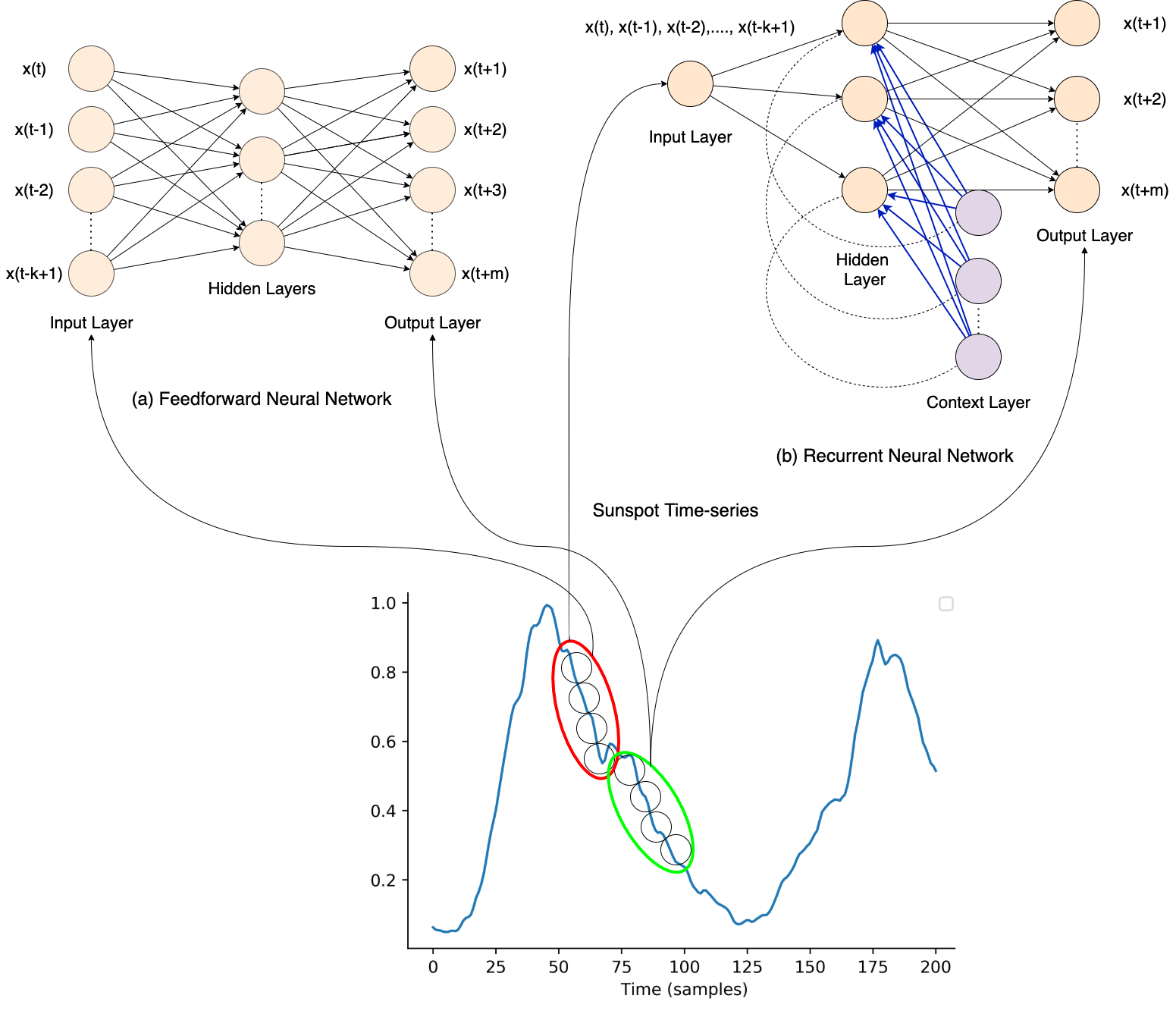
Figure 1: Feedforward neural network and Elman recurrent neural network for time series prediction.

III-D LSTM networks

Simple RNNs have the [23] limitation of learning long-term dependencies with problems in vanishing and exploding gradients [29]. LSTM networks employ memory cells and gates for much better capabilities in remembering the long-term dependencies in temporal sequences as shown in Figure 2. LSTM units are trained in a supervised fashion on a set of training sequences using an adaptation of the BPTT algorithm that considers the respective gates [23]. LSTM networks calculate a hidden state $h_{t}$ as

$$i_{t} =\sigma\big{(}x_{t}U^{i}+h_{t-1}W^{i}\big{)}$$ (3)

$$f_{t} =\sigma\big{(}x_{t}U^{f}+h_{t-1}W^{f}\big{)}$$

$$o_{t} =\sigma\big{(}x_{t}U^{o}+h_{t-1}W^{o}\big{)}$$

$$\tilde{C}_{t} =\tanh\big{(}x_{t}U^{g}+h_{t-1}W^{g}\big{)}$$

$$C_{t} =\sigma\big{(}f_{t}\ast C_{t-1}+i_{t}\ast\tilde{C}_{t}\big{)}$$

$$h_{t} =\tanh(C_{t})\ast o_{t}$$

where, $i_{t}$, $f_{t}$ and $o_{t}$ refer to the input, forget and output gates, at time $t$, respectively. $x_{t}$ and $h_{t}$ refer to the number of input features and number of hidden units, respectively. $W$ and $U$ is the weight matrices adjusted during learning along with $b$ which is the bias. The initial values are $c_{0}=0$ and $h_{0}=0$. All the gates have the same dimensions $d_{h}$, the size of your hidden state. $\tilde{C}_{t}$ is a “candidate” hidden state, and $C_{t}$ is the internal memory of the unit as shown in Figure 2. Note that * denotes element-wise multiplication.

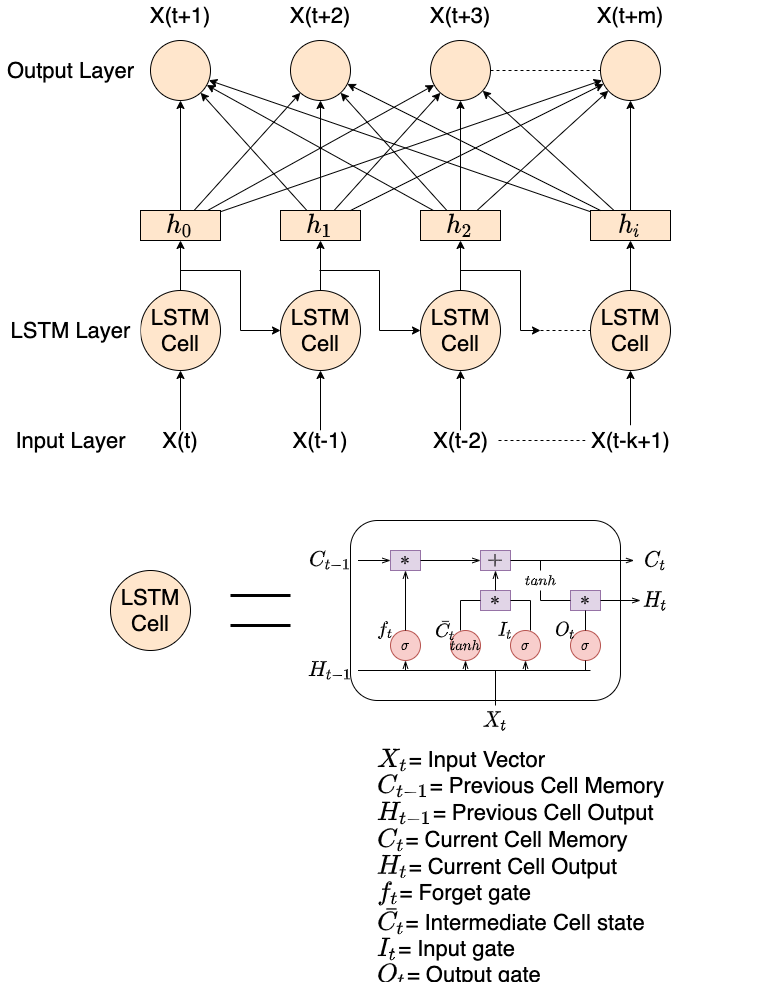
Figure 2: Long Short-Term Memory (LSTM) networks. The LSTM cell denotes memory cells that uses gates and cell memory for remembering long-term dependencies.

III-E Bi-directional LSTM networks

A major shortcoming of conventional RNNs is that they only make use of previous context state for determining future states. Bidirectional RNNs (BD-RNNs) [35] process information in both directions with two separate hidden layers, which are then propagated forward to the same output layer. BD-RNNs consist of placing two independent RNNs together to allow both backward and forward information about the sequence at every time step. BD-RNN computes the forward hidden sequence $h_{f}$, the backward hidden sequence $h_{b}$, and the output sequence $y$ by iterating information from the backward layer, i.e. $t=T$ to $t=1$. Then information in the other network is propagated from $t=1$ to $t=T$ in order to update the output layer; when both networks are combined, information is propagated in bidirectional manner.

Bi-directional LSTM networks (BD-LSTM) [36] have been originally proposed for word-embedding in natural language processing in order to access long-range context or state in both directions, similar to BD-RNNs. BD-LSTM would intake inputs in two ways, one from past to future and one from future to past which differ from conventional LSTM networks. By running information backwards, state information from the future is preserved. Hence, with two hidden states combined, at any point in time the network can preserve information from both past and future as shown in Figure 3. BD-LSTM networks have been used in several real-world sequence processing problems such as phoneme classification [36], continuous speech recognition [87], and speech synthesis [88].

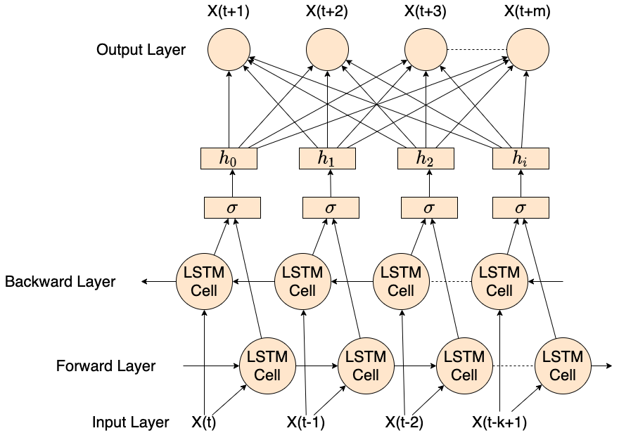
Figure 3: Bi-directional LSTM network.

III-F Encoder-Decoder LSTM networks

Sutskever et al. [89] introduced the encoder-decoder LSTM network (ED-LSTM) which is a sequence to sequence model for mapping a fixed-length input to a fixed-length output [90]. The length of the input and output may differ which makes them applicable in automatic language translation tasks (such as English to French). Hence, the input can be the sequence of video frames $(x_{1},...,x_{n})$, and the output is the sequence of words $(y_{1},...,y_{m})$. Therefore, we estimate the conditional probability of an output sequence $(y_{1},...,y_{m})$, given an input sequence $(x_{1},...,x_{n})$, i.e. $p(y_{1},...,y_{m}|x_{1},...,x_{n})$. In the case of multi-step series prediction, both the input and outputs are of variable lengths. ED-LSTM networks handle variable-length input and outputs by first encoding the input sequences one at a time, using a latent vector representation, and then decoding them from that representation. In the encoding phase, given an input sequence, the ED-LSTM computes a sequence of hidden states. In the decoding phase, it defines a distribution over the output sequence given the input sequence as shown in Figure 4.

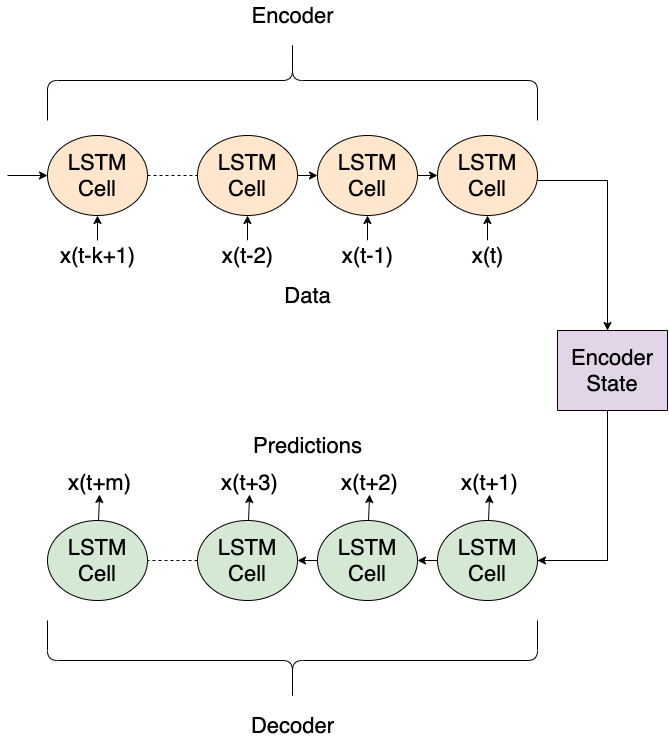
Figure 4: Encoder-Decoder LSTM network.

III-G CNNs

CNNs introduced by LeCun [91, 92] are prominent deep learning architecture inspired by the natural visual system of mammals. CNNs can be trained using backpropagation algorithm for tasks such as handwritten digit classification [93]. CNNs have been prominent in many computer vision and image processing tasks. Recently, CNNs have been applied for time series prediction and produced very promising results [77, 76, 75]. CNNs learn spatial hierarchies of features by using multiple building blocks, such as convolution, pooling layers, and fully connected layers. Figure 5 shows an example of a CNN used for time series prediction using a univariate time series as input where multiple output neurons represent different prediction horizons. We note that CNNs are more appropriate for multivariate time series with use of features extracted via the convolutional and the pooling layers.

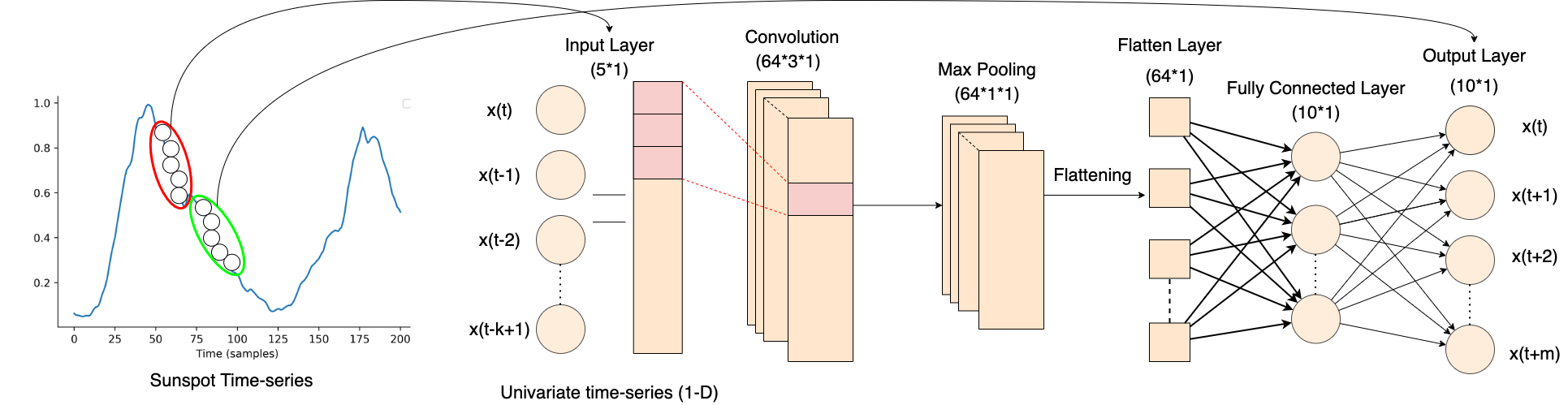
Figure 5: One-dimensional convolutional neural network for multi-step ahead time series prediction.

IV Experiments and Results

IV-A Experimental Design

We use a combination of benchmark problems that include simulated and real-world time series. The simulated time series are Mackey-Glass[94], Lorenz [95], Henon [96], and Rossler [97]. The real-world time series are Sunspot [98], Lazer [99] and ACI-financial time series [100]. They have been used in our previous works and have been prominent for time series problems [101, 102, 103]. The Sunspot time series indicates solar activities from November 1834 to June 2001 and consists of 2000 data points [98]. The ACI-finance time series contains closing stock prices from December 2006 to February 2010, featuring 800 data points [100]. The Lazer time series is from the Santa Fe competition that consists of 500 points [99].

The respective time series are processed into a state-space vector [83] with embedding dimension $D=5$ and time-lag $T=1$ for 10-step-ahead prediction. We determine respective model hyper-parameters from trial experiments that include number of hidden neurons, and learning rate. Table I gives details for the topology of the respective models in terms of input, hidden and output layers. We use maximum time of 1000 epochs with rectifier linear units (Relu) in all the respective models. The simple neural networks feature SGD and Adam optimiser (FNN-SGD and FNN-Adam). Adam optimiser is used in the deep learning models that include simple RNNs, LSTM networks, ED-LSTM, BD-LSTM, and CNNs.

The time series are scaled in the range [0,1]. We used first 1000 data points from which the first 60% are used for training and remaining for testing. We use the root-mean-squared error (RMSE) as the main performance measure ( Equation 4) for the different prediction horizons

$$RMSE=\sqrt{\frac{1}{N}\sum_{i=1}^{N}(y_{i}-\hat{y}_{i})^{2}}$$ (4)

where, $y_{i},\hat{y}_{i}$ are the observed data, predicted data, respectively. $N$ is the length of the observed data.

TABLE I: Configuration of models

	Input	Hidden Layers	Output	Comments
FNN-Adam	5	1	10	Hidden layer = 10 neurons
FNN-SGD	5	1	10	Hidden layer = 10 neurons
LSTM	5	1	10	Hidden layer = 10 cells
BD-LSTM	5	1	10	Forward and backward layer = 10 cells each
ED-LSTM	5	4	10	Two LSTM networks with a time distributed layer
RNN	5	2	10	Hidden layer = 10 neurons
CNN	5	4	10	Filters=64, convolutional window size=3, and max-pooling window size=2

IV-B Results

We report the mean and 95 % confidence interval of RMSE for each prediction horizon for the respective problem for train and test datasets from 30 experimental runs with different initial neural network weights. Figure 9 to Figure 12 presents the results for the simulated time series (Tables VIII to XI in Appendix). Figure 6 to 8 presents the results for the real-world time series (Tables V to VII in Appendix). We define robustness as the confidence interval which must be as low as possible to indicate high confidence in prediction. We consider scalability as the ability to provide consistent performance as the the prediction horizon increases. The results are given in terms of the RMSE where the lower values indicate better performance. Each problem reports 10-step-ahead prediction results with RMSE mean and 95% confidence interval as error bars, shown in Figures 6 to 12.

We first review results for real-world time series that feature noise (ACI-Finance, Sunspot, Lazer). Figure 6 shows the results for the ACI-fiancee problem. We observe that the test performance is better than the train performance in Figure 6 (a), where deep learning models provide more reliable performance. The prediction error (RMSE) increases with the prediction horizon, and the deep learning methods do much better than simple neural networks (FNN-SGD and FNN-Adam). We find that LSTM provides the best overall performance as shown in Figure 6 (b). The overall test performance shown in Figure 6 (a) indicates that FNN-Adam and LSTM provide similar performance, which are better than rest of the problems. Figure 13 shows ACI-finance prediction performance of the best experiment run with selected prediction horizons that indicate how the prediction deteriorates as prediction horizon increases.

Next, we consider the results for the Sunspot time series shown in Figure 7 which follows a similar trend as the ACI-finance problem in terms of the increase in prediction error along with the prediction horizon. The test performance is better than the train performance as evident from Figure 7 (a). The LSTM methods (LSTM, ED-LSTM, BD-LSTM) gives better performance than the other methods as can be observed from Figure 7 (a) and 7 (b). Note that the FNN-SGD gives the worst performance and the performance of RNN is better than that of CNN, FNN-SGD, and FNN-Adam, but poorer than LSTM methods. Figure 14 shows Sunspot prediction performance of the best experiment run with selected prediction horizons.

The results for Lazer time series is shown in Figure 8, which exhibits a similar trend in terms of the train and test performance as the other real-world time series problems. Note that the Lazer problem is highly chaotic (as visually evident in Figure 16), which seems to be the primary reason behind the difference in performance for the prediction horizon in contrast to other problems as displayed in Figure 8 (b). It is striking that none of the methods appear to be showing any trend for the prediction accuracy along the prediction horizon, as seen in previous problems. In terms of scalability, all the methods appear to be performing better in comparison with the other problems. The performance of CNN is better than that of RNN, which is different from other real-world time series. Figure 16 shows Lazer prediction performance of the best experiment run using ED-LSTM with selected prediction horizons. We note that due to the chaotic nature of the time series, the prediction performance is visually not clear.

We now consider simulated time series that do not feature noise (Henon, Mackey-Glass, Rosssler, Lorenz). The Henon time series in Figure 9 shows that ED-LSTM provides the best performance. Note that there is a more significant difference between the three LSTM methods when compared to other problems. The trends are similar to the ACI-finance and the Sunspot problem given the prediction horizon performance in Figure 9 (a) and 9 (b), where the simple neural networks (FNN-SGD and FNN-Adam) appear to be more scalable than the other methods along the prediction horizon, although they perform poorly. Figure 17 and Figure 15 show Mackey-Glass and Henon prediction performance of the best experiment run using ED-LSTM for selected prediction horizons. The Henon prediction in Figure 15 indicates that it is far more chaotic than Mackey-Glass; hence, it faces more challenges. We show them since these are cases with no noise when compared to real-world time series previously shown. They have a larger deterioration in prediction performance as the prediction horizon increases (Figures 13 and Figure 14).

In the Lorenz, Mackey-Glass and Rossler simulated time series, the deep learning methods are performing far better than the simple neural networks as shown in Figures 10, 11 and 12. The trend along the prediction horizon is similar to previous problems, i.e., the prediction error increases along with the prediction horizon. If we consider scalability, the deep learning methods are more scalable in the Lorenz, Mackey-Glass and Rossler problems than the previous problems. This is the first instance where the CNN has outperformed LSTM for Mackey-Glass and Rossler time series.

We note that there have been distinct trends in prediction for the different types of problems. In the simulated time series, given that we exclude Henon, we observe a similar trend for Mackey-Glass, Lorenz and Rossler time series. The trend indicates that simple neural networks face major difficulties. ED-LSTM and BD-LSTM networks provides the best performance, which also applies to Henon time series, except that it has close performance for simple neural networks when compared to deep learning models for 7-10 prediction horizons (Figure 9 b). This difference reflects in the nature of the time series which is highly chaotic in nature (Figure 15). We further note that in the case of the simple neural networks, Henon (Figure 9) does not deteriorate in performance as the prediction horizon increases when compared to Mackley-Glass, Lorenz and Rossler problems. Simple neural networks in this case performs poorly from the beginning prediction horizon.

The performance of simple neural networks in Lazer problem shows a similar trend in Lazer time series, where the predictions are poor from the beginning and its striking that LSTM networks actually improve the performance as the prediction horizon increases (Figure 8 b). This trend is a clear outlier when compared to the rest of real-world and simulated problems, since they all show deep learning models deteriorate as the prediction horizon increases.

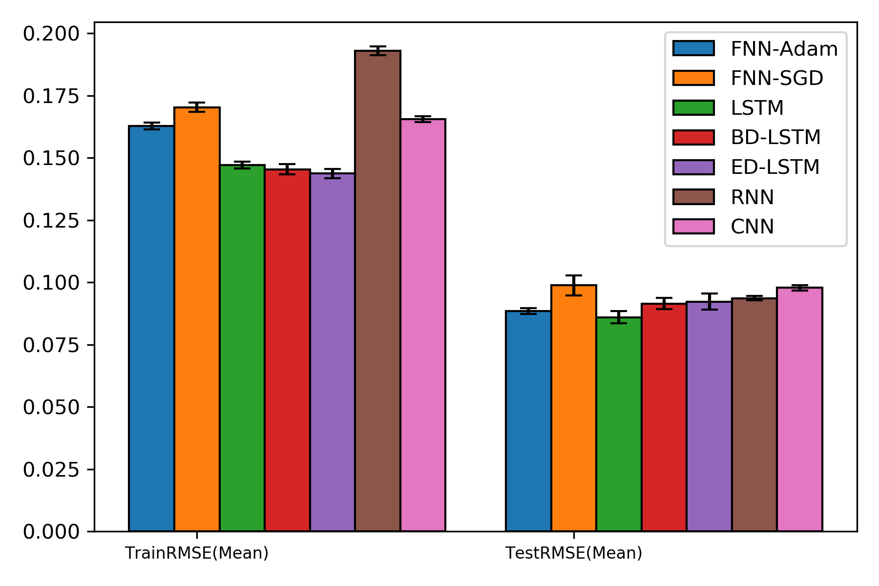
(a) RMSE across 10 prediction horizons

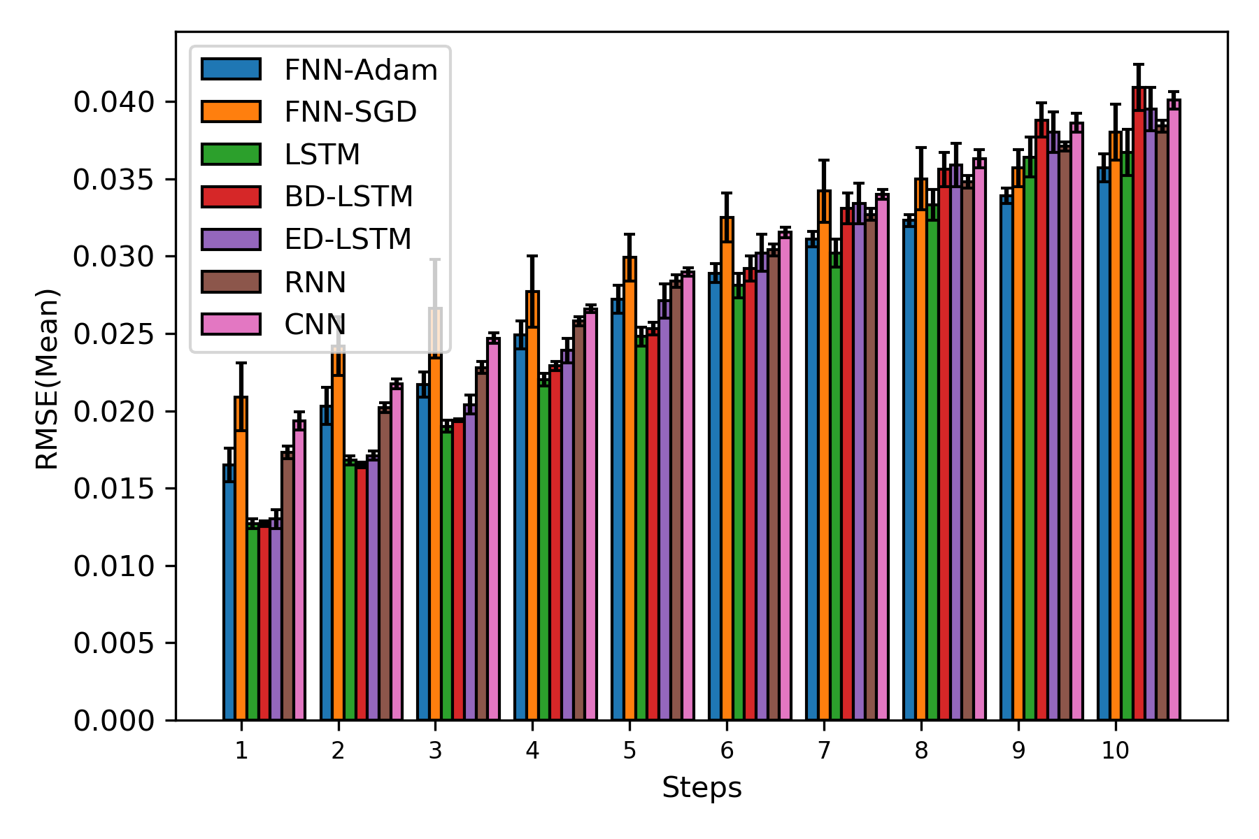
(b) 10 step-ahead prediction

Figure 6: ACI-finance time series: performance evaluation of respective methods (RMSE mean and 95% confidence interval as error bar).

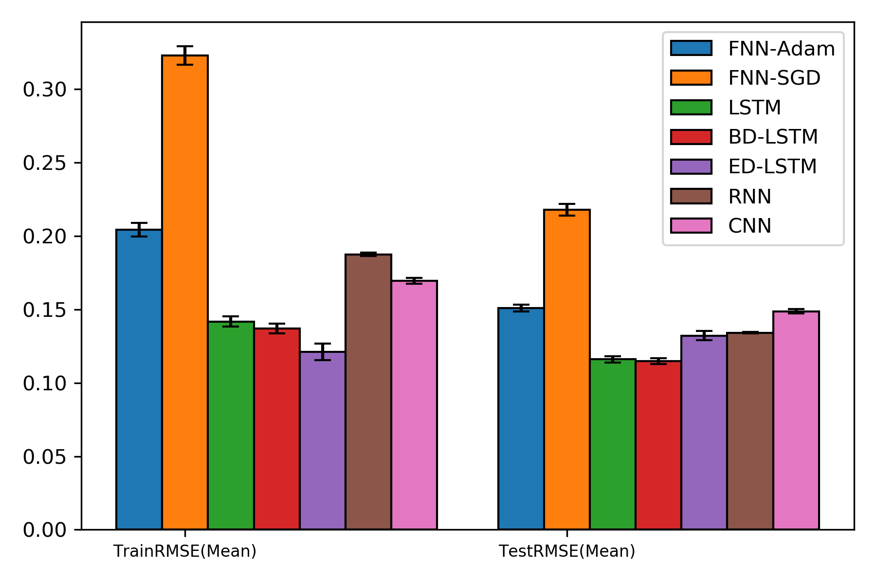
(a) RMSE across 10 prediction horizons

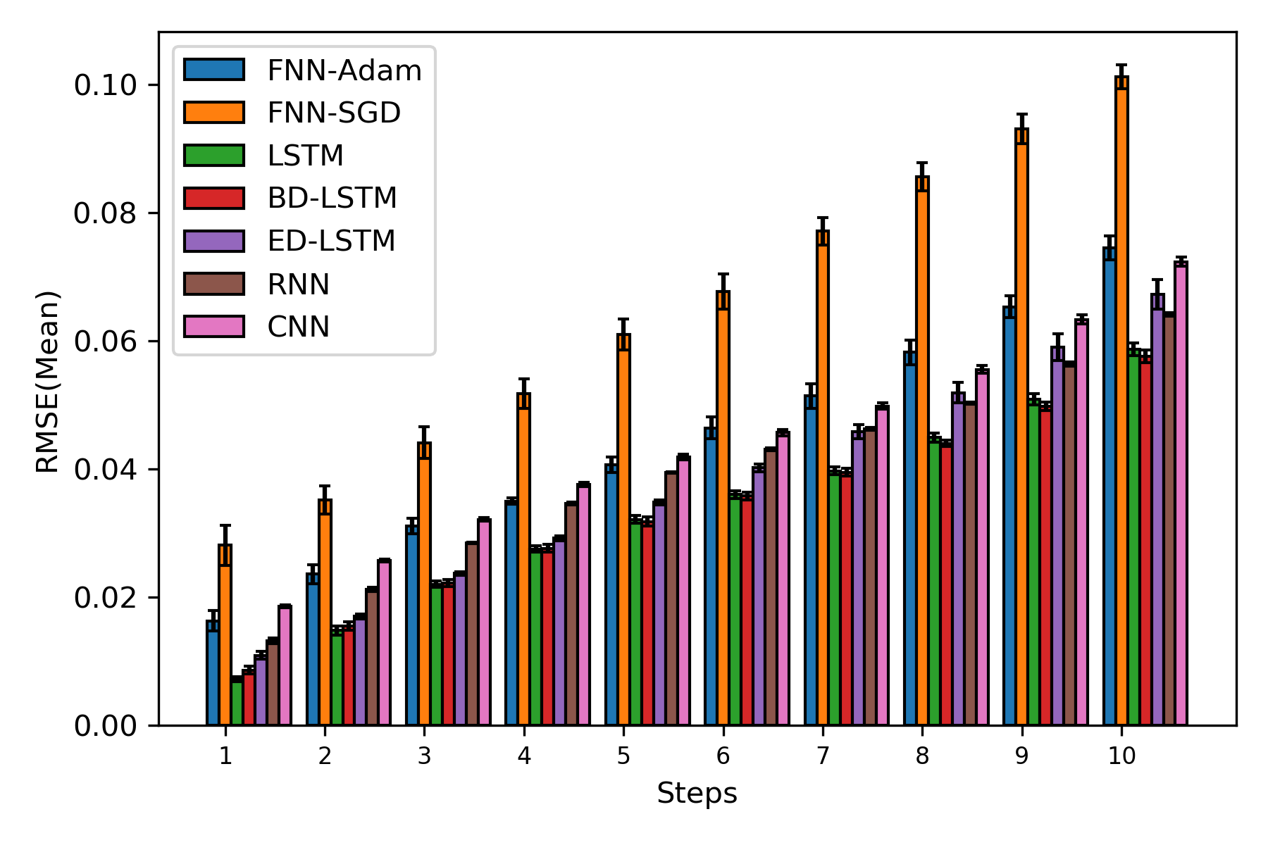
(b) 10 step-ahead prediction

Figure 7: Sunspot time series: performance evaluation of respective methods (RMSE mean and 95% confidence interval as error bar).

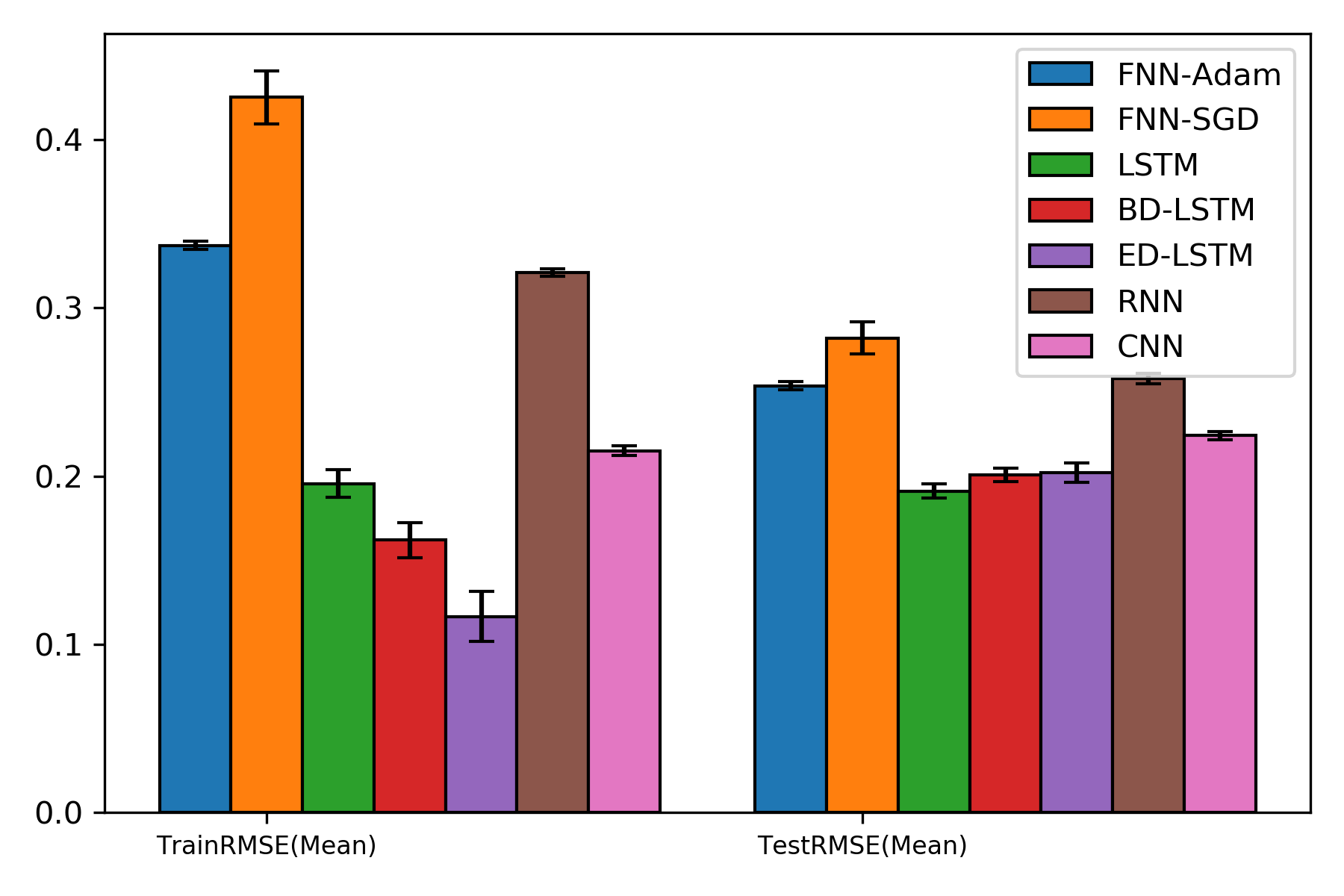
(a) RMSE across 10 prediction horizons

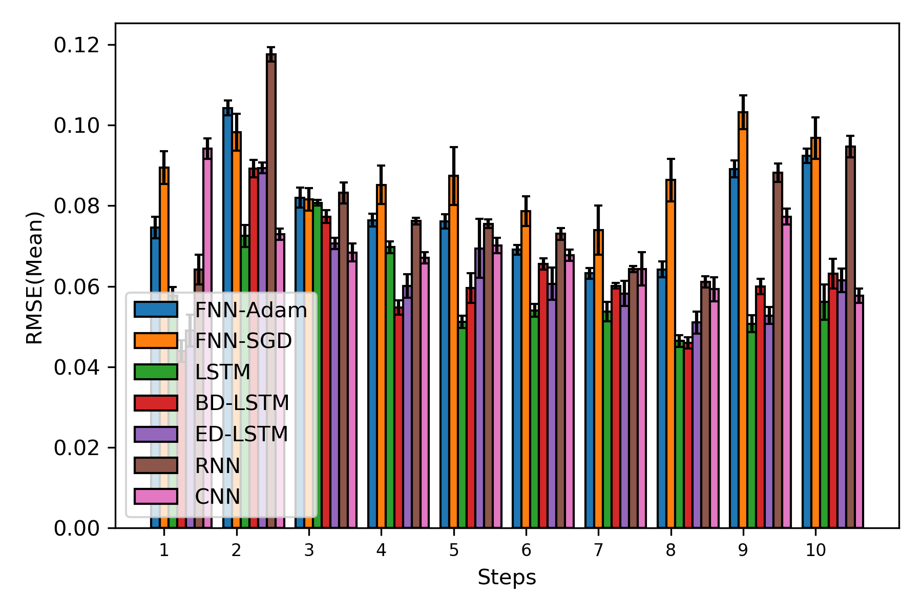
(b) 10 step-ahead prediction

Figure 8: Lazer time series: performance evaluation of respective methods (RMSE mean and 95% confidence interval as error bar).

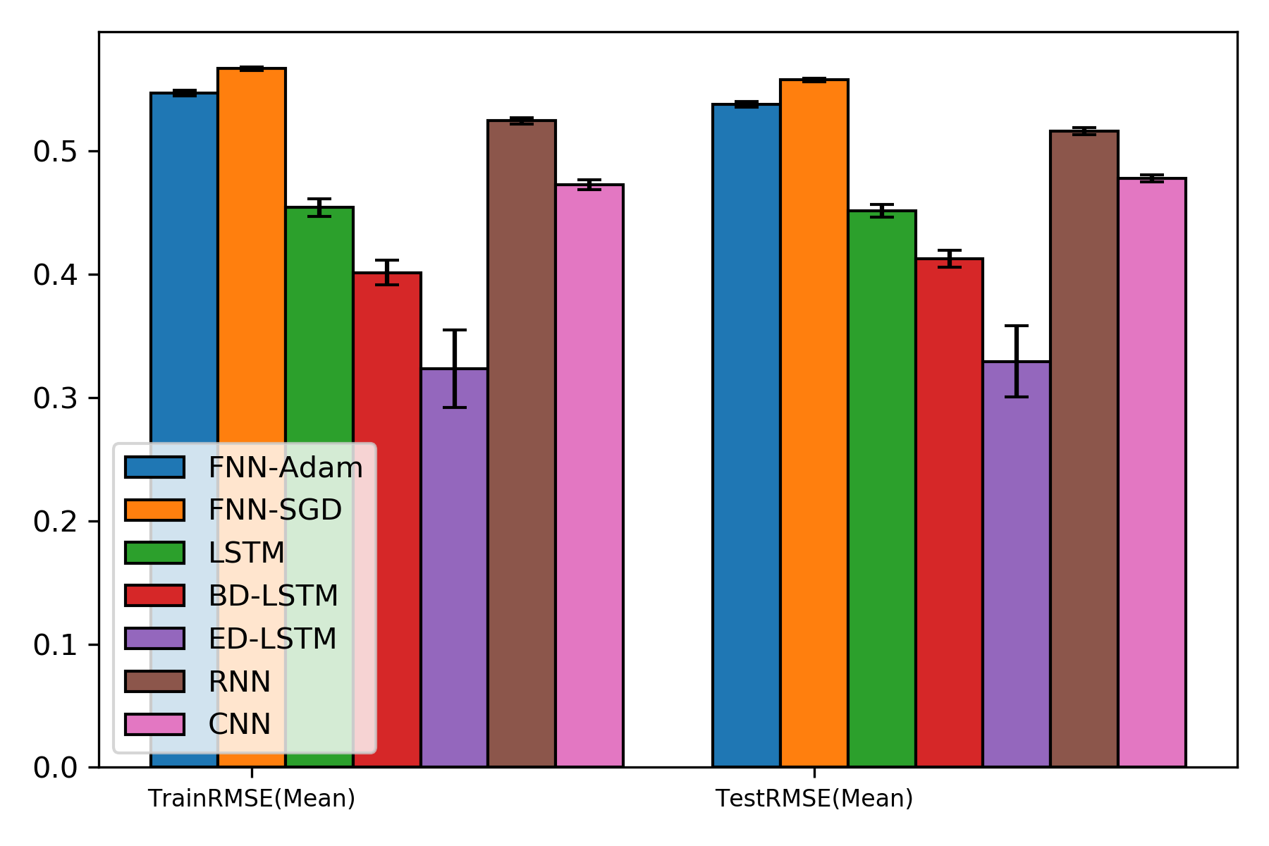
(a) RMSE-Mean

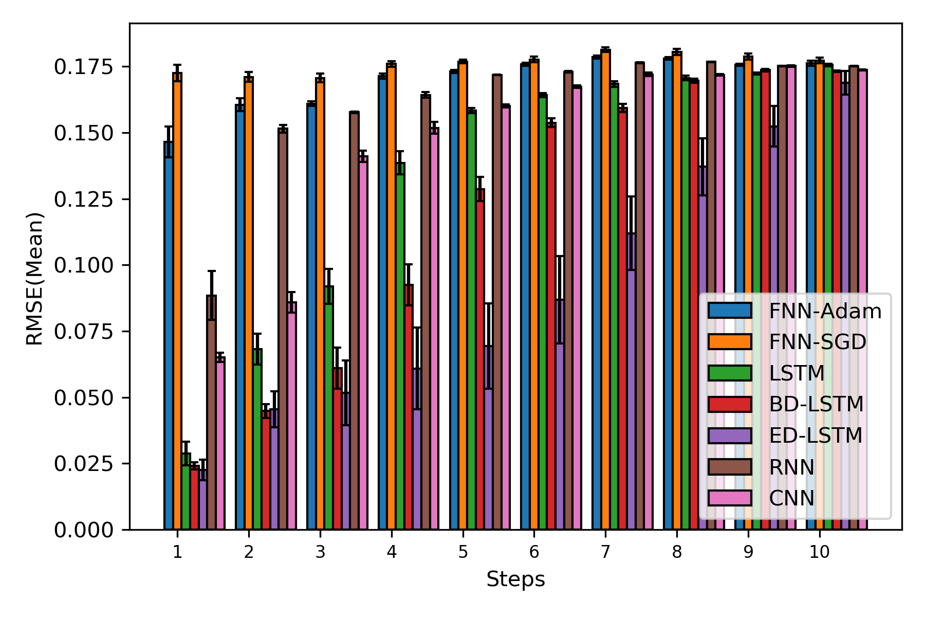
(b) 10 step-ahead prediction

Figure 9: Henon time series: performance evaluation of respective methods (RMSE mean and 95% confidence interval as error bar).

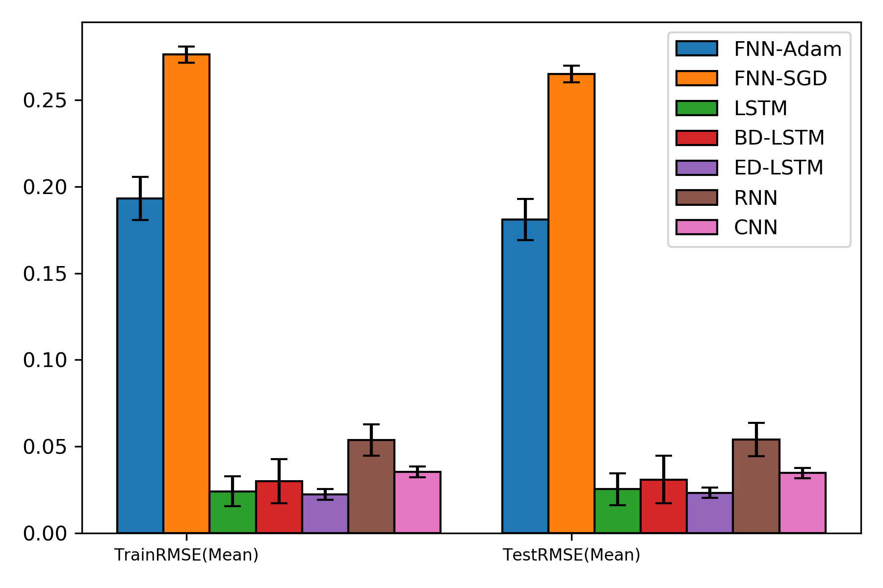
(a) RMSE across 10 prediction horizons

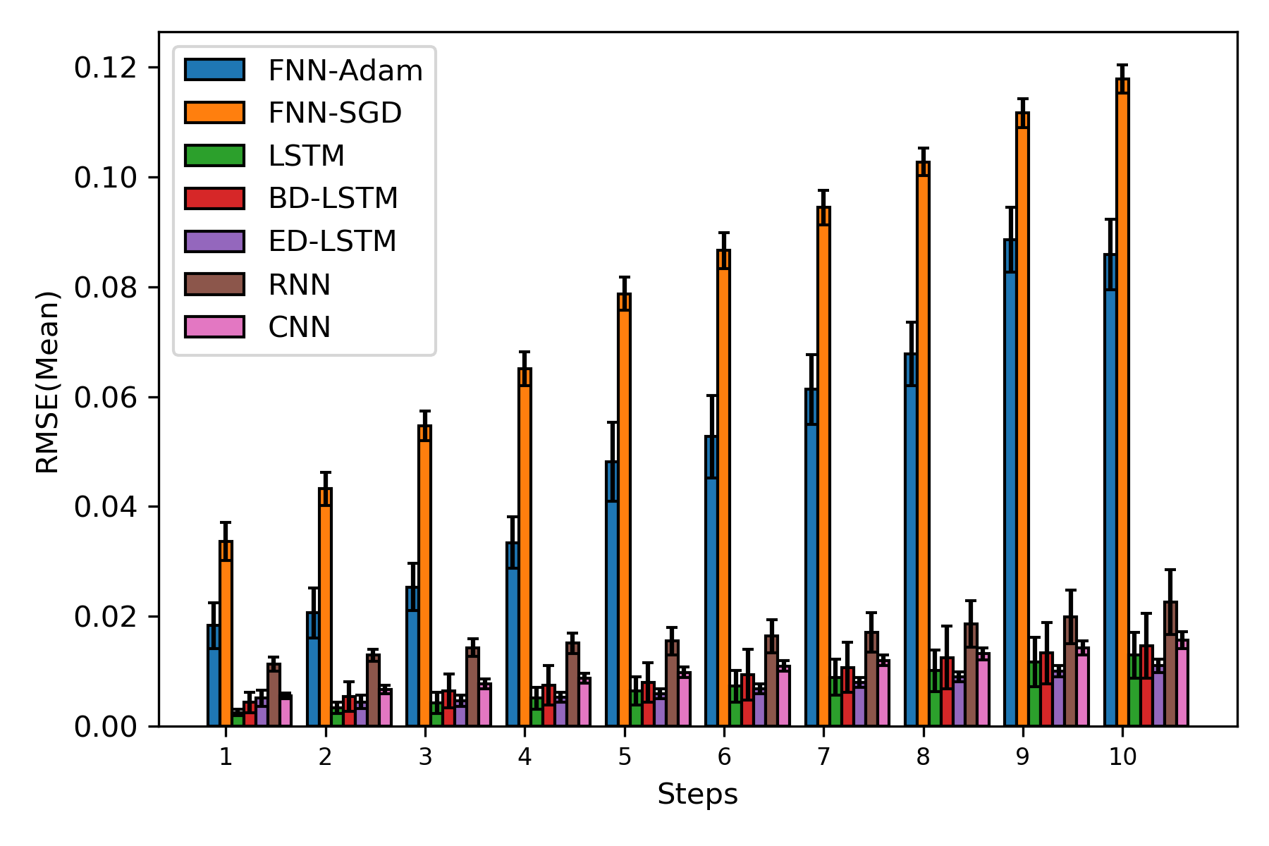
(b) 10 step-ahead prediction

Figure 10: Lorenz time series: performance evaluation of respective methods (RMSE mean and 95% confidence interval as error bar).

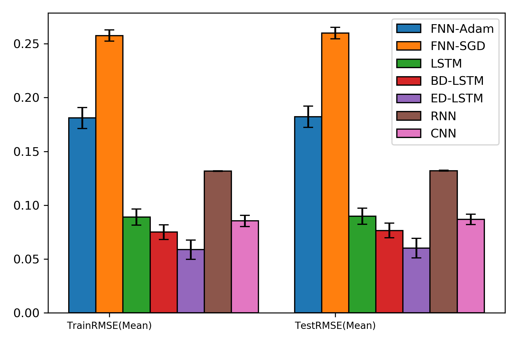
(a) RMSE across 10 prediction horizons

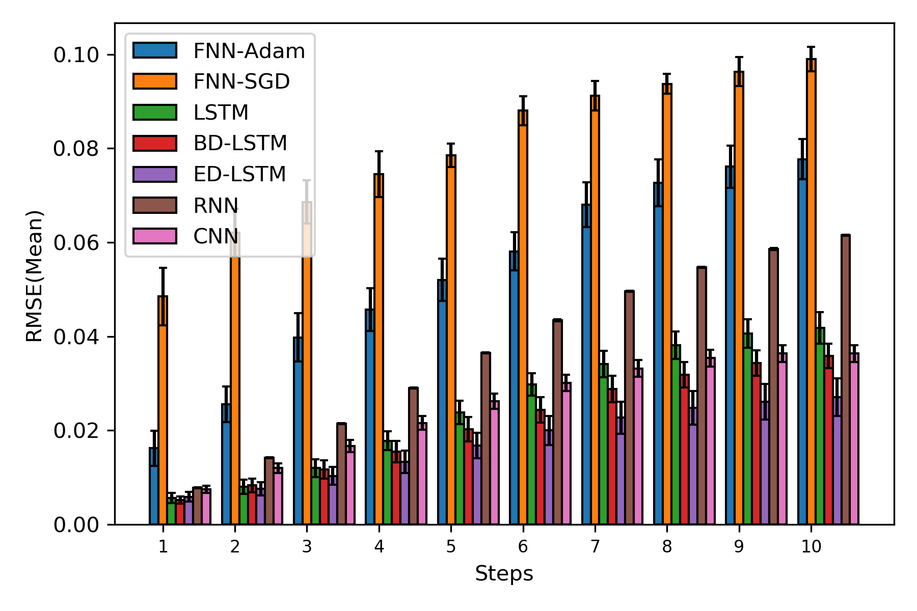
(b) 10 step-ahead prediction

Figure 11: Mackey-Glass time series: performance evaluation of respective methods (RMSE mean and 95% confidence interval as error bar).

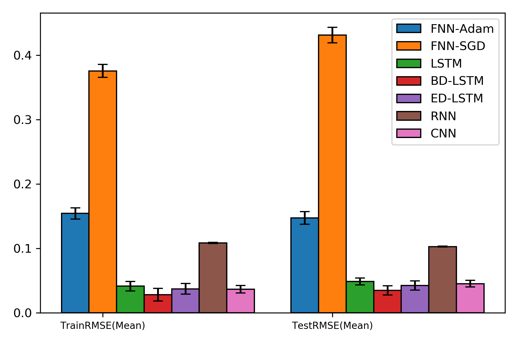
(a) RMSE across 10 prediction horizons

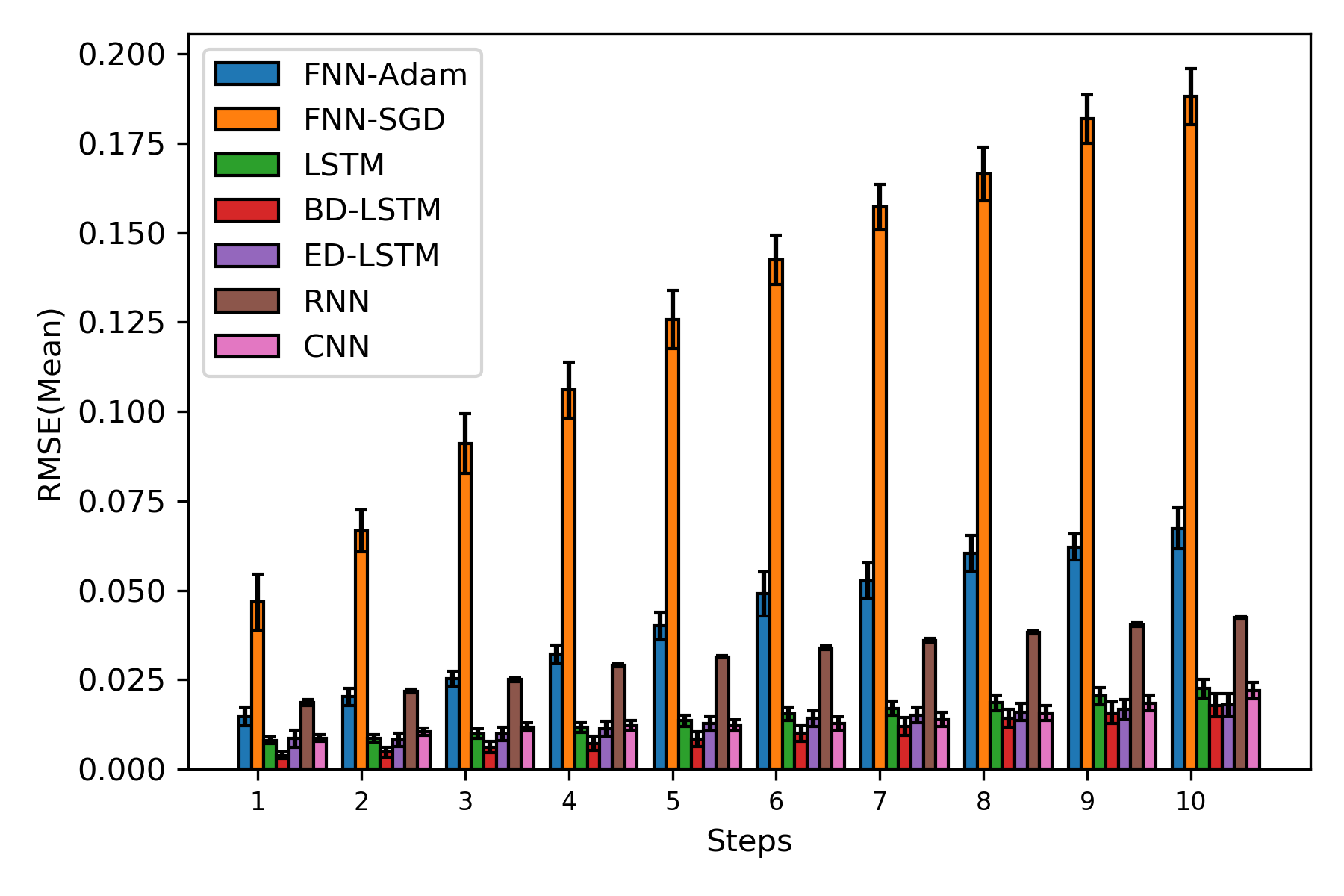
(b) 10 step-ahead prediction

Figure 12: Rossler time series: performance evaluation of respective methods (RMSE mean and 95% confidence interval as error bar).

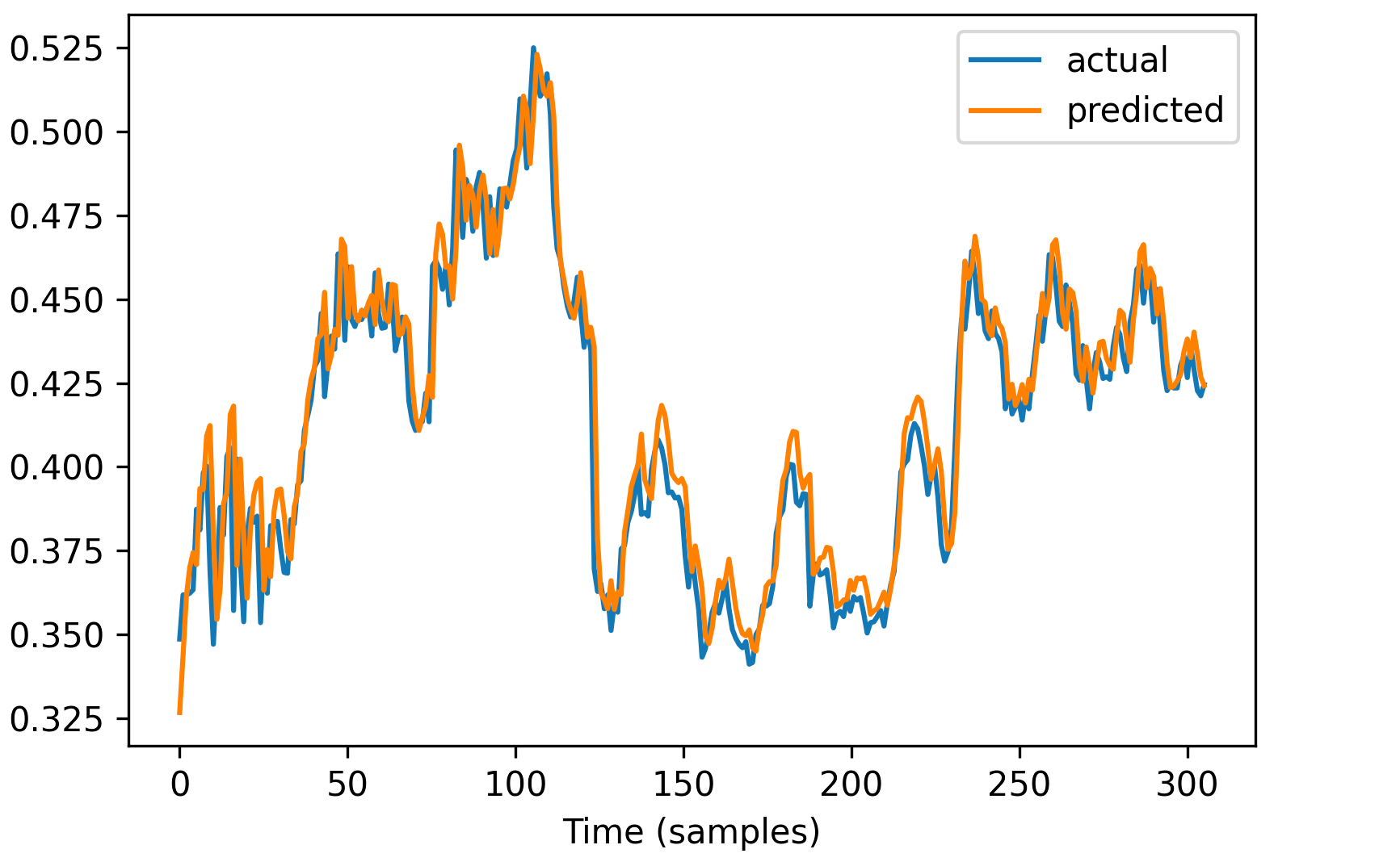
(a) Step 1

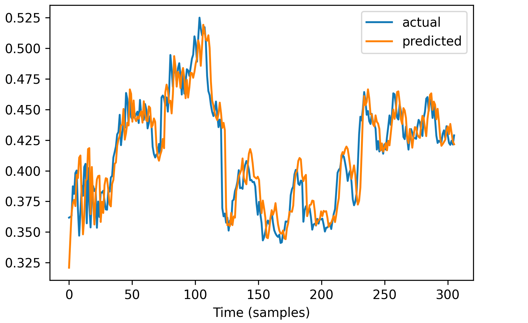
(b) Step 3

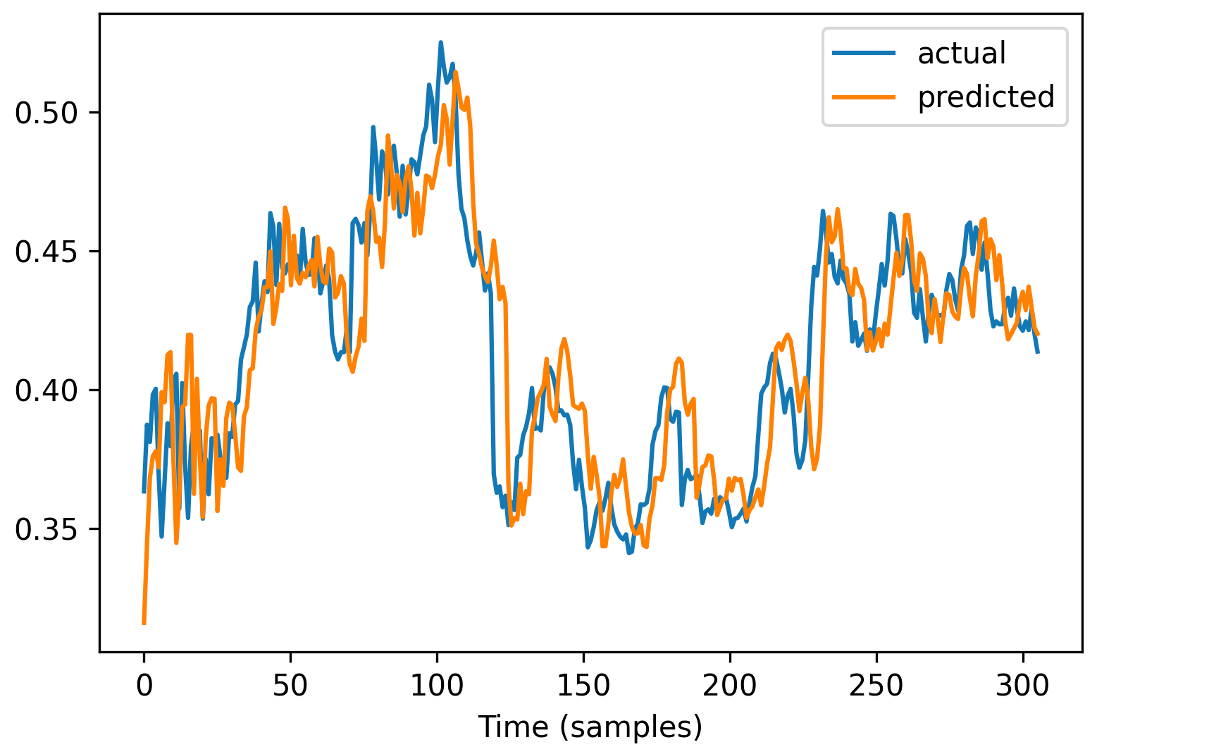
(c) Step 5

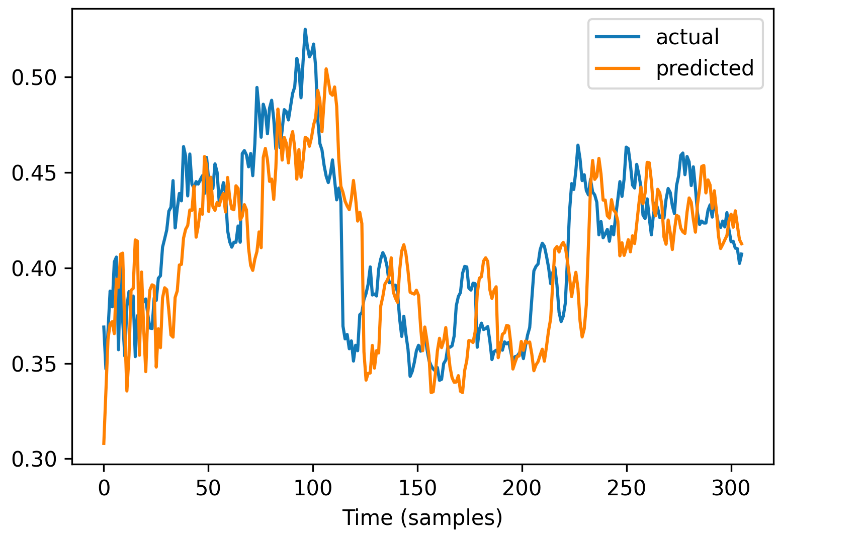
(d) Step 10

Figure 13: ACI-finance actual vs predicted values for Encoder-Decoder LSTM Model

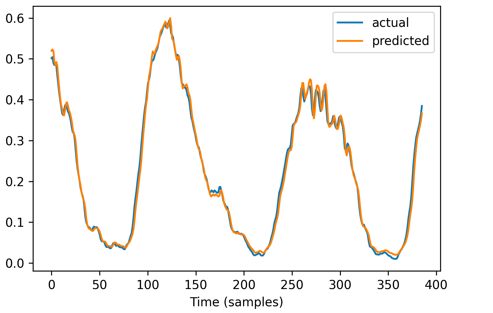
(a) Step 1

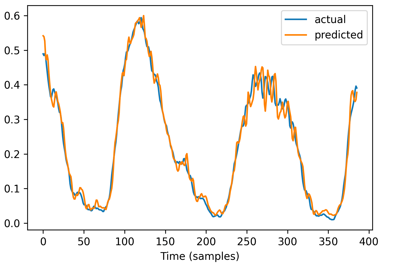
(b) Step 3

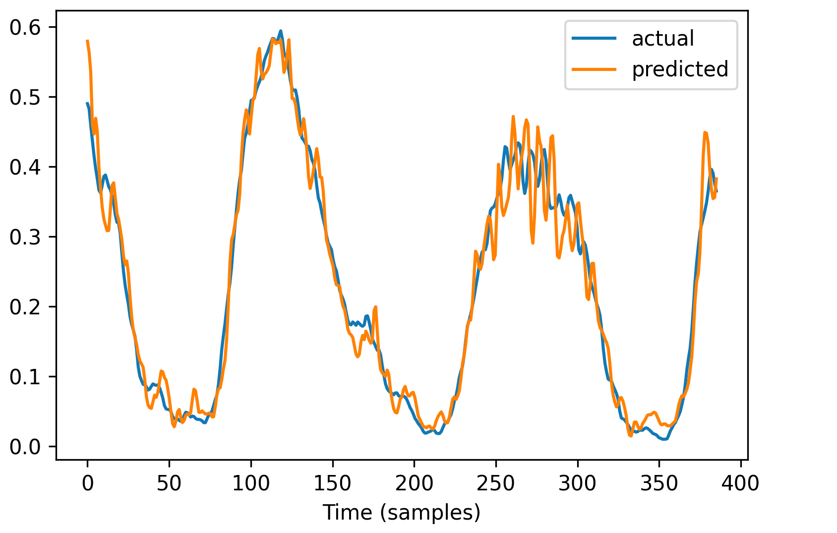
(c) Step 5

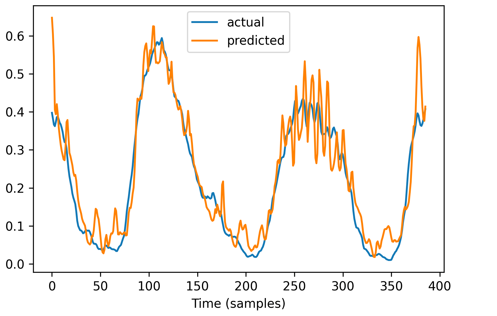
(d) Step 10

Figure 14: Sunspot actual vs predicted values for Encoder-Decoder LSTM Model

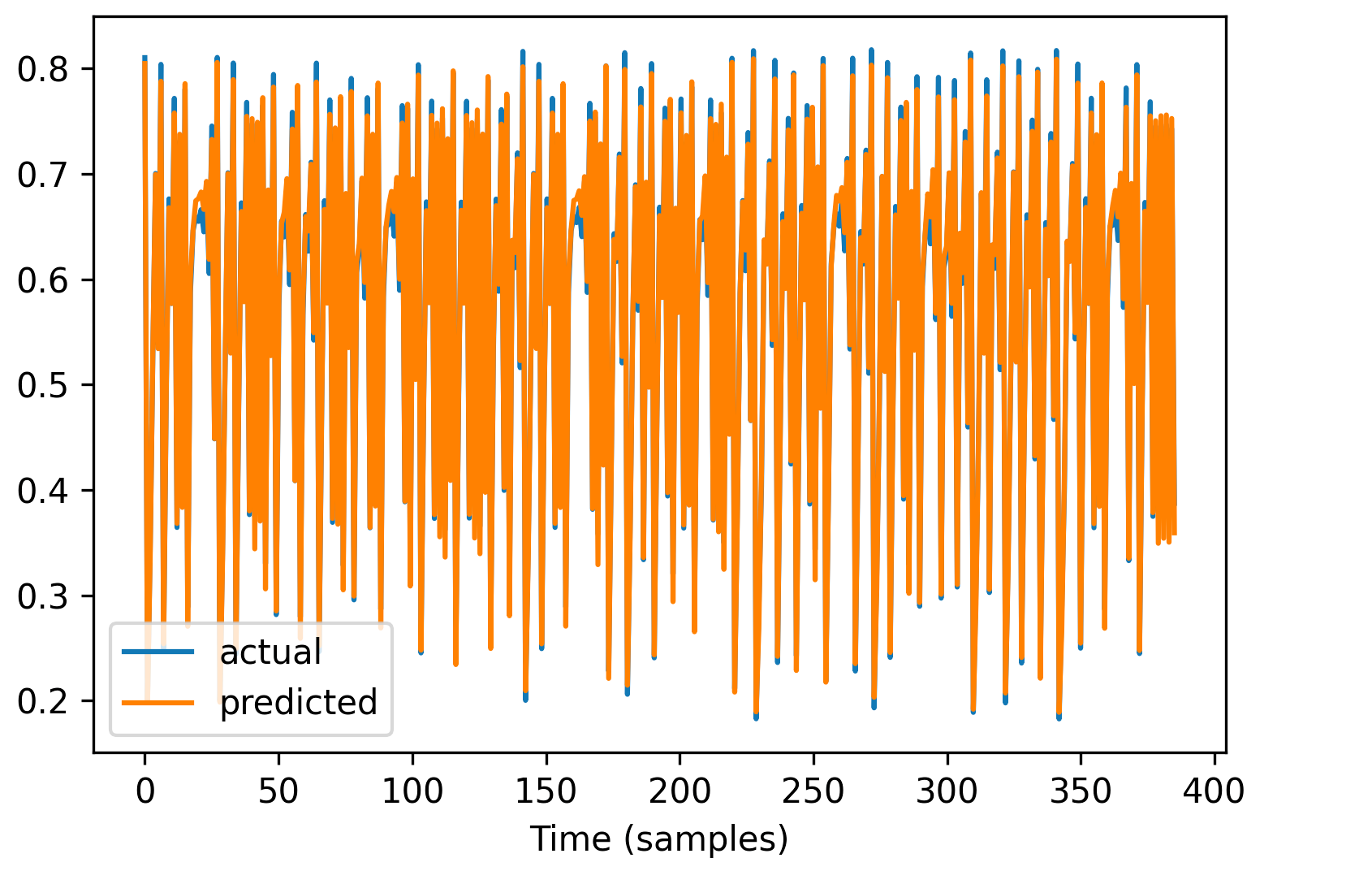
(a) Step 1

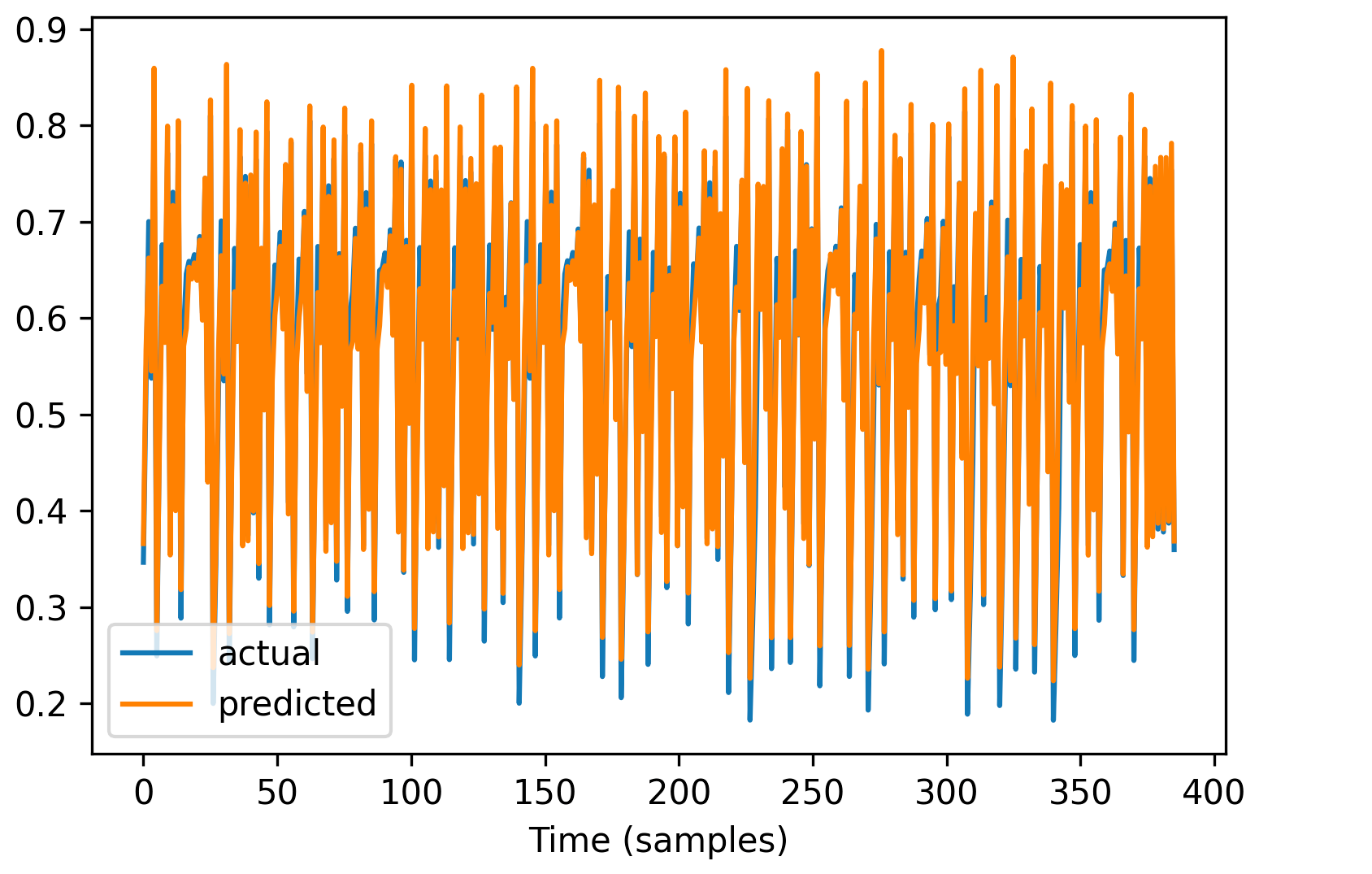
(b) Step 3

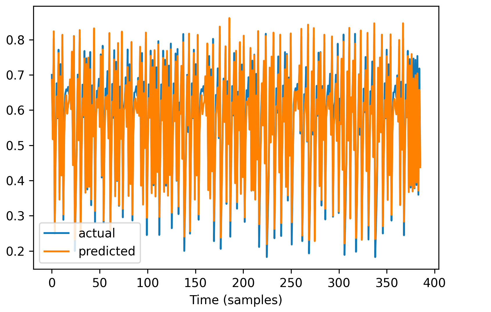
(c) Step 5

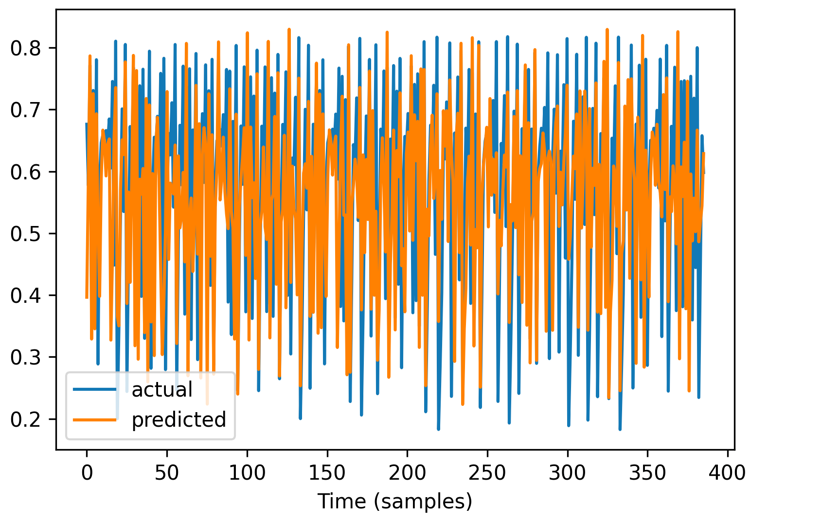
(d) Step 10

Figure 15: Henon actual vs predicted values for Encoder-Decoder LSTM Model

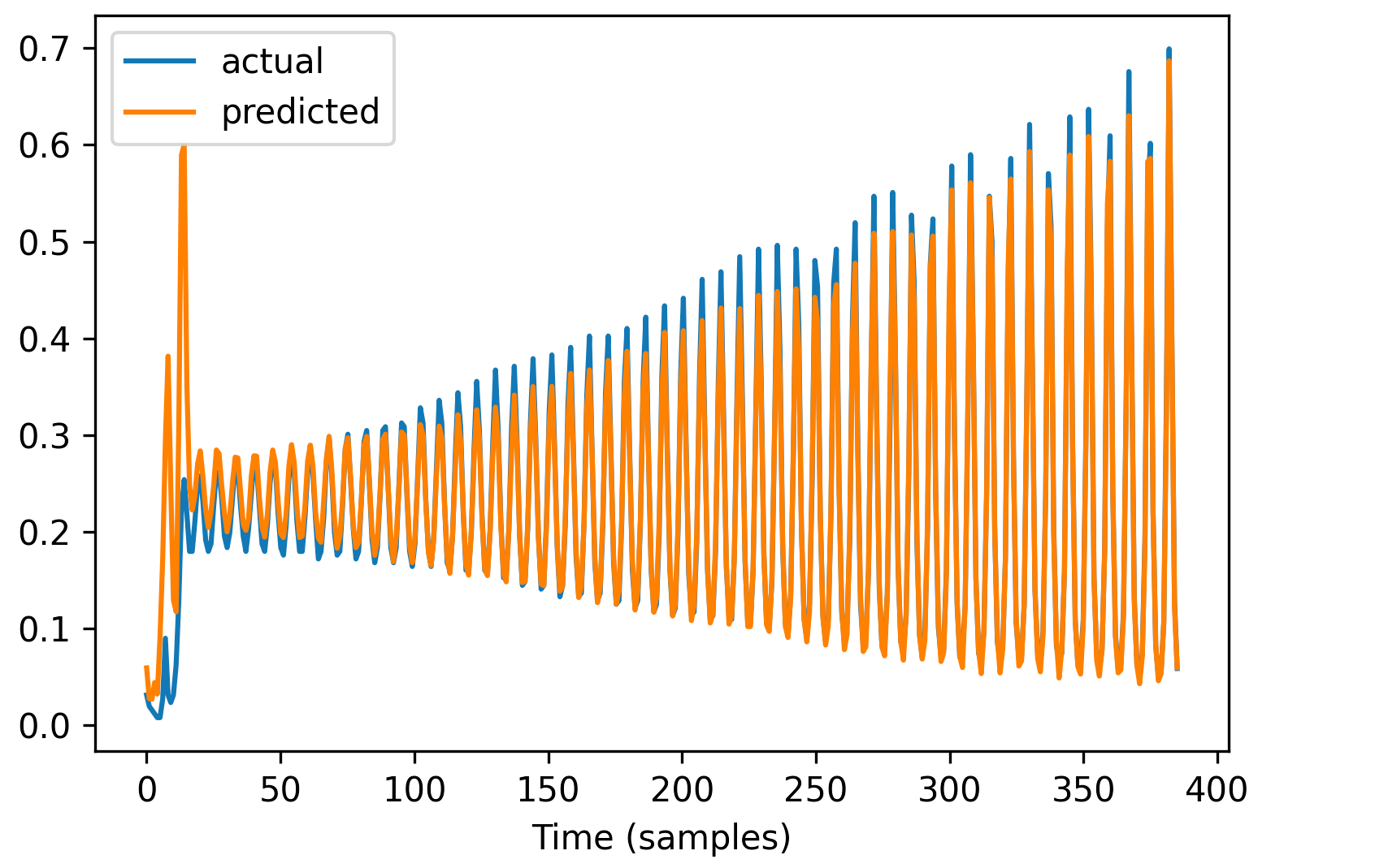
(a) Step 1

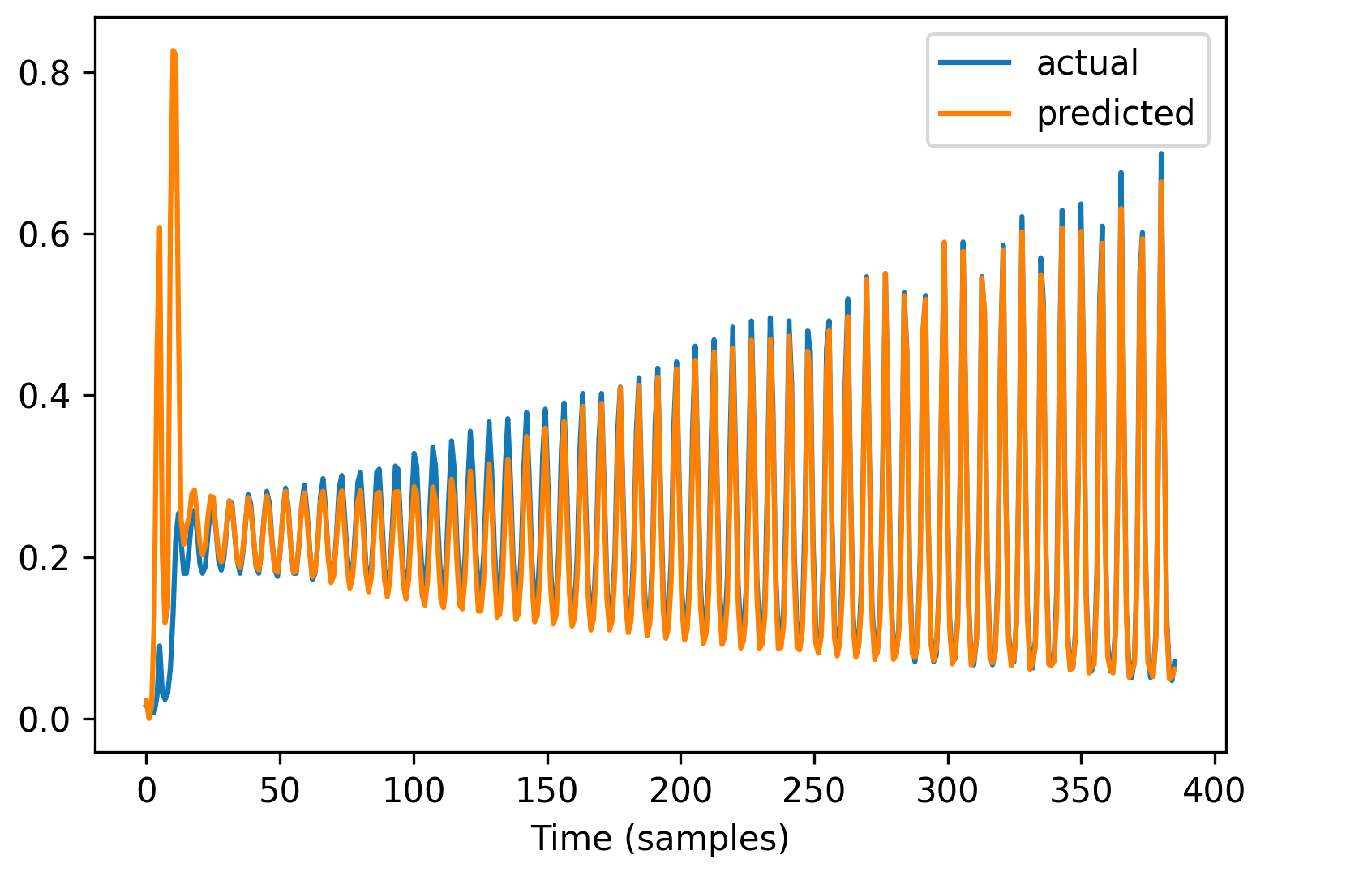
(b) Step 3

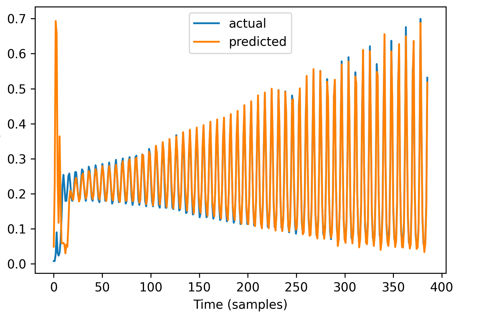
(c) Step 5

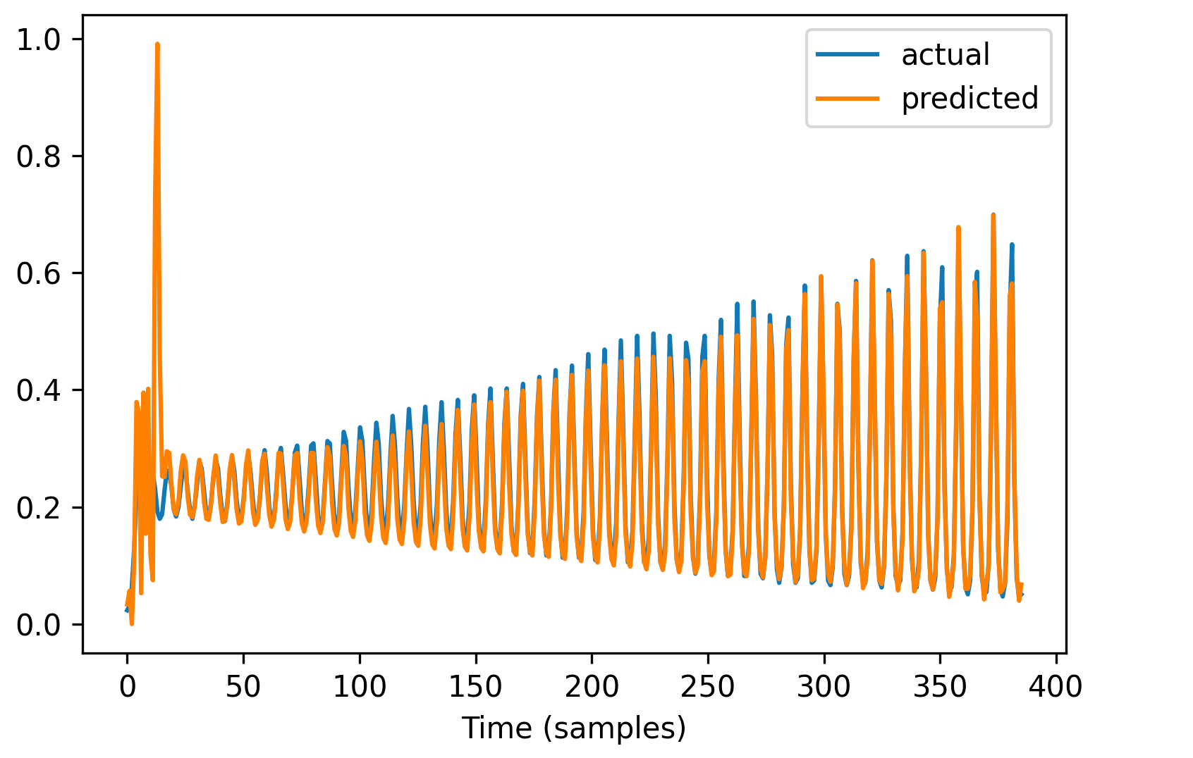
(d) Step 10

Figure 16: Lazer actual vs predicted values for Encoder-Decoder LSTM Model

(a) Step 1

(b) Step 3

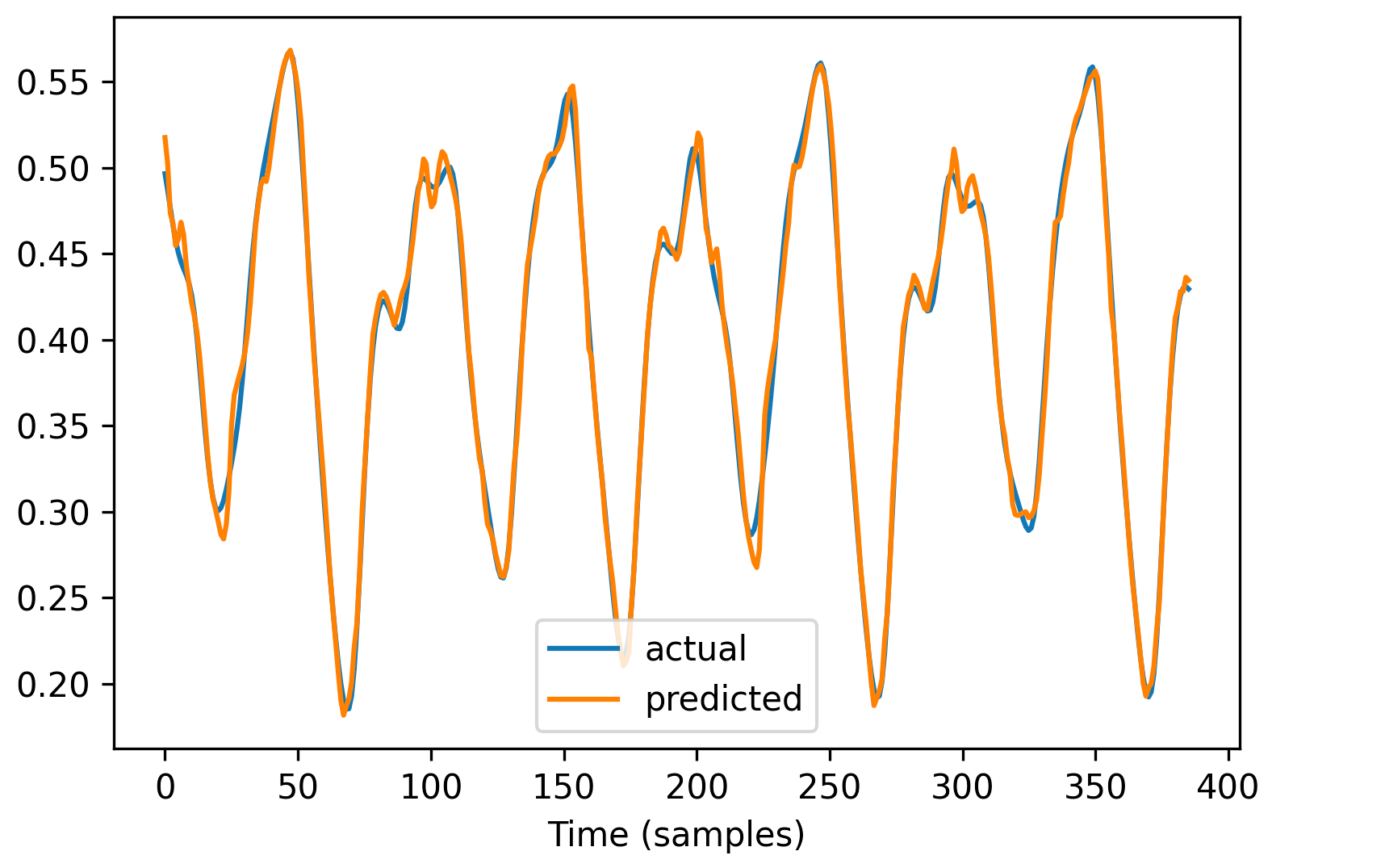
(c) Step 5

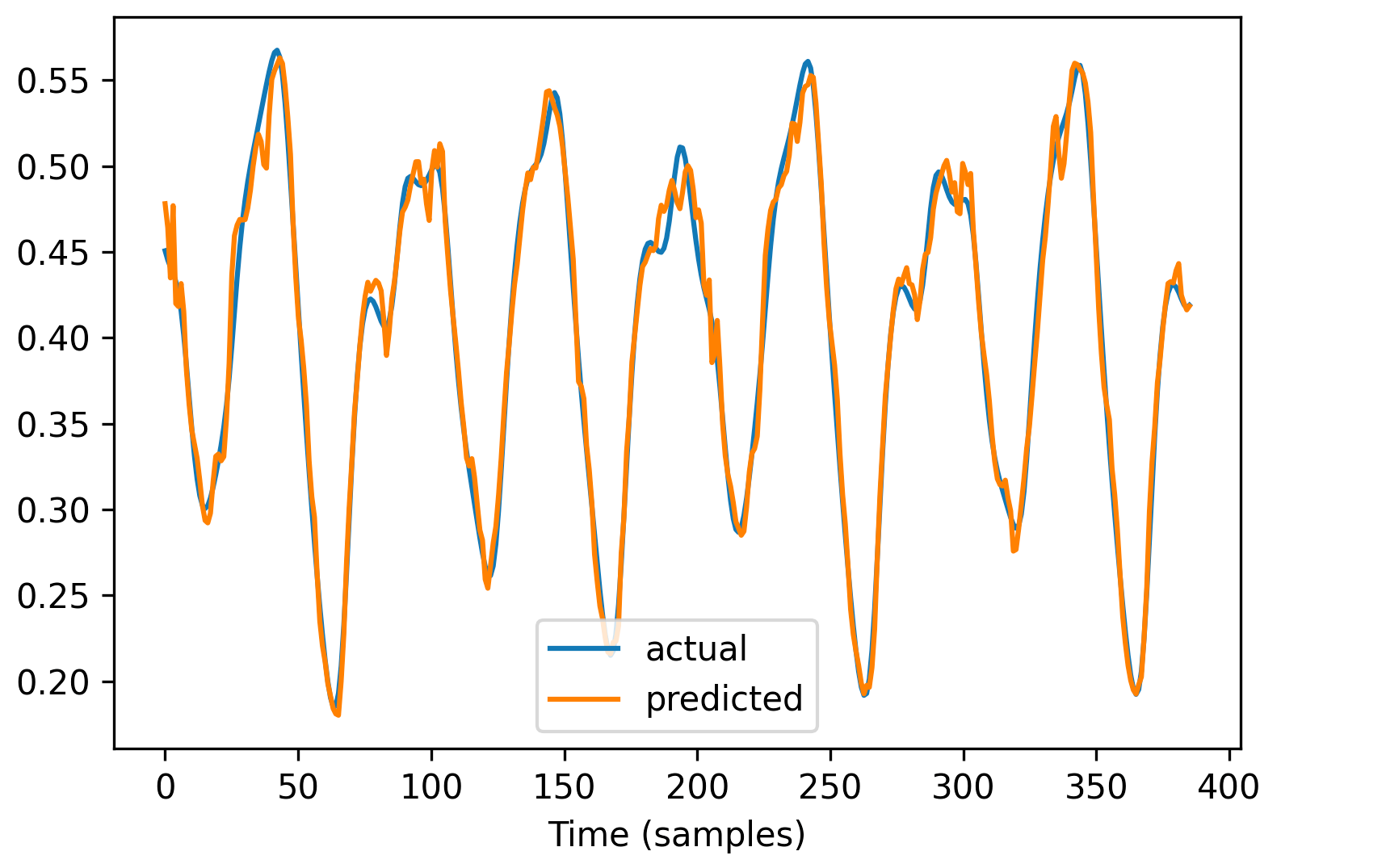
(d) Step 10

Figure 17: Mackey-Glass actual vs predicted values for Encoder-Decoder LSTM Model

TABLE II: Performance (rank) of different models for respective time-series problems. Note lower rank denotes better performance.

	FNN-Adam	FNN-SGD	LSTM	BD-LSTM	ED-LSTM	RNN	CNN
ACI-finance	2	7	1	3	4	5	6
Sunspot	6	7	2	1	3	4	5
Lazer	6	7	1	2	3	5	4
Henon	6	7	3	2	1	5	4
Lorenz	6	7	2	3	1	5	4
Mackey-Glass	6	7	4	2	1	5	1
Rossler	6	7	4	1	2	5	3
Mean-Rank	5.42	7.00	2.42	2.00	2.14	4.85	3.85

IV-C Comparison with the literature

TABLE III: Comparison with Literature for Simulated time series.

Problem	Method	2-step	5-step	8-step	10 steps
Mackey-Glass
	2SA-RTRL* [12]	0.0035
	ESN*[12]	0.0052
	EKF[104]		0.2796
	G-EKF [104]		0.2202
	UKF [104]		0.1374
	G-UKF [104]		0.0509
	GPF[104]		0.0063
	G-GPF[104]		0.0022
	Multi-KELM[54]	0.0027	0.0031	0.0028	0.0029
	MultiTL-KELM[54]	0.0025	0.0029	0.0026	0.0028
	CMTL [52]	0.0550	0.0750	0.0105	0.1200
	ANFIS(SL) [105]	0.0051	0.0213	0.0547
	R-ANFIS(SL) [105]	0.0045	0.0195	0.0408
	R-ANFIS(GL) [105]	0.0042	0.0127	0.0324
	FNN-Adam	0.0256$\pm$ 0.0038	0.0520$\pm$ 0.0044	0.0727$\pm$ 0.0050	0.0777$\pm$ 0.0043
	FNN-SGD	0.0621$\pm$ 0.0051	0.0785$\pm$ 0.0025	0.0937$\pm$ 0.0022	0.0990$\pm$ 0.0026
	LSTM	0.0080$\pm$ 0.0014	0.0238$\pm$ 0.0024	0.0381$\pm$ 0.0029	0.0418$\pm$ 0.0033
	BD-LSTM	0.0083$\pm$ 0.0015	0.0202$\pm$ 0.0026	0.0318$\pm$ 0.0027	0.0359$\pm$ 0.0026
	ED-LSTM	0.0076$\pm$ 0.0014	0.0168$\pm$ 0.0027	0.0248$\pm$ 0.0036	0.0271$\pm$ 0.0040
	RNN	0.0142$\pm$ 0.0001	0.0365$\pm$ 0.0001	0.0547$\pm$ 0.0001	0.0615$\pm$ 0.0001
	CNN	0.0120$\pm$ 0.0010	0.0262$\pm$ 0.0016	0.0354$\pm$ 0.0018	0.0364$\pm$ 0.0017
Lorenz
	2SA-RTRL*[12]	0.0382
	ESN*[12]	0.0476
	CMTL [52]	0.0490	0.0550	0.0710	0.0820
	FNN-Adam	0.0206$\pm$ 0.0046	0.0481$\pm$ 0.0072	0.0678$\pm$ 0.0058	0.0859$\pm$ 0.0065
	FNN-SGD	0.0432$\pm$ 0.0030	0.0787$\pm$ 0.0030	0.1027$\pm$ 0.0025	0.1178$\pm$ 0.0026
	LSTM	0.0033$\pm$ 0.0010	0.0064$\pm$ 0.0026	0.0101$\pm$ 0.0038	0.0129$\pm$ 0.0042
	BD-LSTM	0.0054$\pm$ 0.0026	0.0079$\pm$ 0.0036	0.0125$\pm$ 0.0057	0.0146$\pm$ 0.0059
	ED-LSTM	0.0044$\pm$ 0.0012	0.0059$\pm$ 0.0009	0.0090$\pm$ 0.0009	0.0110$\pm$ 0.0012
	RNN	0.0129$\pm$ 0.0012	0.0155$\pm$ 0.0024	0.0186$\pm$ 0.0042	0.0226$\pm$ 0.0058
	CNN	0.0067 $\pm$0.0007	0.0098$\pm$ 0.0009	0.0132$\pm$ 0.0011	0.0157$\pm$ 0.0015
Rossler
	CMTL [52]	0.0421	0.0510	0.0651	0.0742
	FNN-Adam	0.0202$\pm$ 0.0024	0.0400$\pm$ 0.0039	0.0603$\pm$ 0.0050	0.0673$\pm$ 0.0056
	FNN-SGD	0.0666$\pm$ 0.0058	0.1257$\pm$ 0.0082	0.1664$\pm$ 0.0075	0.1881$\pm$ 0.0078
	LSTM	0.0086$\pm$ 0.0011	0.0135$\pm$ 0.0015	0.0185$\pm$ 0.0022	0.0225$\pm$ 0.0026
	BD-LSTM	0.0047$\pm$ 0.0014	0.0084$\pm$ 0.0021	0.0142$\pm$ 0.0027	0.0178$\pm$ 0.0032
	ED-LSTM	0.0082$\pm$ 0.0019	0.0128$\pm$ 0.0021	0.0159$\pm$ 0.0024	0.0180$\pm$ 0.0030
	RNN	0.0218$\pm$ 0.0005	0.0314$\pm$ 0.0004	0.0382$\pm$ 0.0004	0.0424$\pm$ 0.0004
	CNN	0.0105$\pm$ 0.0011	0.0122$\pm$ 0.0016	0.0157$\pm$ 0.0020	0.0220$\pm$ 0.0022
Henon
	Multi-KELM[54]	0.0041	0.2320	0.2971	0.2968
	MultiTL-KELM[54]	0.0031	0.1763	0.2452	0.2516
	CMTL [52]	0.2103	0.2354	0.2404	0.2415
	FNN-Adam	0.1606 $\pm$ 0.0024	0.1731 $\pm$ 0.0005	0.1781 $\pm$ 0.0005	0.1762 $\pm$ 0.0009
	FNN-SGD	0.1711 $\pm$ 0.0018	0.1769 $\pm$ 0.0007	0.1805 $\pm$ 0.0012	0.1773 $\pm$ 0.0011
	LSTM	0.0682 $\pm$ 0.0058	0.1584 $\pm$ 0.0010	0.1707 $\pm$ 0.0008	0.1756 $\pm$ 0.0005
	BD-LSTM	0.0448 $\pm$ 0.0026	0.1287 $\pm$ 0.0046	0.1697 $\pm$ 0.0008	0.1733 $\pm$ 0.0003
	ED-LSTM	0.0454 $\pm$ 0.0069	0.0694 $\pm$ 0.0161	0.1371 $\pm$ 0.0107	0.1689 $\pm$ 0.0046
	RNN	0.1515$\pm$ 0.0016	0.1718 $\pm$ 0.0001	0.1768 $\pm$ 0.0001	0.1751 $\pm$ 0.0002
	CNN	0.0859 $\pm$ 0.0038	0.1601$\pm$ 0.0007	0.1718$\pm$ 0.0003	0.1737$\pm$ 0.0002

TABLE IV: Comparison with Literature for Real World time series.

Problem	Method	2-step	5-step	8-step	10-step
Lazer
	CMTL [52]	0.0762	0.1333	0.1652	0.1885
	FNN-Adam	0.1043 $\pm$ 0.0018	0.0761 $\pm$ 0.0019	0.0642 $\pm$ 0.0020	0.0924$\pm$ 0.0018
	FNN-SGD	0.0983 $\pm$ 0.0046	0.0874 $\pm$ 0.0072	0.0864$\pm$ 0.0053	0.0968$\pm$ 0.0052
	LSTM	0.0725 $\pm$ 0.0027	0.0512 $\pm$ 0.0015	0.0464$\pm$ 0.0015	0.0561$\pm$ 0.0044
	BD-LSTM	0.0892 $\pm$ 0.0022	0.0596 $\pm$ 0.0036	0.0460$\pm$ 0.0015	0.0631$\pm$ 0.0037
	ED-LSTM	0.0894 $\pm$ 0.0013	0.0694 $\pm$ 0.0073	0.0510$\pm$ 0.0027	0.0615$\pm$ 0.0030
	RNN	0.1176 $\pm$ 0.0019	0.0755 $\pm$ 0.0011	0.0611$\pm$ 0.0015	0.0947$\pm$ 0.0027
	CNN	0.0729$\pm$ 0.0014	0.0701$\pm$ 0.0020	0.0593$\pm$ 0.0029	0.0577$\pm$ 0.0018
Sunspot
	M-SVR [14]				0.2355 $\pm$ 0.0583
	SVR-I [14]				0.2729 $\pm$0.1414
	SVR-D [14]				0.2151 $\pm$ 0.0538
	CMTL [52]	0.0473	0.0623	0.0771	0.0974
	FNN-Adam	0.0236$\pm$ 0.0015	0.0407$\pm$ 0.0012	0.0582$\pm$ 0.0019	0.0745$\pm$ 0.0020
	FNN-SGD	0.0352$\pm$ 0.0022	0.0610$\pm$ 0.0024	0.0856$\pm$ 0.0023	0.1012$\pm$ 0.0019
	LSTM	0.0148$\pm$ 0.0007	0.0321$\pm$ 0.0006	0.0449$\pm$ 0.0007	0.0587$\pm$ 0.0010
	BD-LSTM	0.0155$\pm$ 0.0007	0.0318$\pm$ 0.0007	0.0440$\pm$ 0.0005	0.0576$\pm$ 0.0010
	ED-LSTM	0.0170$\pm$ 0.0004	0.0348$\pm$ 0.0004	0.0519$\pm$ 0.0016	0.0673$\pm$ 0.0022
	RNN	0.0212$\pm$ 0.0003	0.0395$\pm$ 0.0002	0.0503$\pm$ 0.0002	0.0641$\pm$ 0.0003
	CNN	0.0257$\pm$ 0.0002	0.0419 $\pm$0.0004	0.0555$\pm$ 0.0006	0.0723$\pm$ 0.0008
ACI-Finance
	CMTL [52]	0.0486	0.0755	0.08783	0.1017
	FNN-Adam	0.0203 $\pm$ 0.0012	0.0272 $\pm$ 0.0008	0.0323 $\pm$ 0.0004	0.0357 $\pm$ 0.0008
	FNN-SGD	0.0242 $\pm$ 0.0020	0.0299 $\pm$ 0.0015	0.0350 $\pm$ 0.0021	0.0380 $\pm$ 0.0018
	LSTM	0.0168 $\pm$ 0.0003	0.0248 $\pm$ 0.0006	0.0333 $\pm$ 0.0010	0.0367$\pm$ 0.0015
	BD-LSTM	0.0165 $\pm$ 0.0002	0.0253 $\pm$ 0.0004	0.0356 $\pm$ 0.0010	0.0409 $\pm$ 0.0015
	ED-LSTM	0.0171 $\pm$ 0.0003	0.0271 $\pm$ 0.0010	0.0359 $\pm$ 0.0014	0.0395 $\pm$ 0.0014
	RNN	0.0202 $\pm$ 0.0003	0.0284 $\pm$ 0.0004	0.0348 $\pm$ 0.0004	0.0384 $\pm$ 0.0003
	CNN	0.0217 $\pm$0.0004	0.0290 $\pm$0.0002	0.0363 $\pm$0.0006	0.0401$\pm$ 0.0005

Tables III and IV show a comparison with related methods from the literature for simulated and real-world time series, respectively. We note that the comparison is not fair as other methods may have employed different models with different data processing and also in reporting of results with different measures of error. Moreover, some papers report best experimental run and do not show mean and standard deviation of the results. We highlight in bold the best performance for respective prediction horizon. In Table III, we compare the Mackey-Glass and Lorenz time series performance for two-step-ahead prediction by real-time recurrent learning (RTRL) and echo state networks (ESN) [12]. Note that * in the results implies that the comparison is not fair due to different embedding dimension in state-space reconstruction and it is not clear if the mean or the best run has been reported. We show further comparison for Mackey-Glass for 5th prediction horizon using Extended Kalman Filtering (EKF), the Unscented Kalman Filtering (UKF) and the Gaussian Particle Filtering (GPF), along with their generalized versions G-EKF, G-UKF and G-GPF, respectively [104]. In the case of MultiTL-KELM [54], we find that it beats all our proposed methods for Mackey-Glass, except for the Henon time series. In general, we find that our proposed deep learning methods (LSTM, BD-LSTM, ED-LSTM) outperform most of the methods from the literature for the simulated time series, except for the Mackey-Glass time series.

In Table IV, we compare the performance of Sunspot time series with support vector regression (SVR), iterated (SVR-I), direct (SVR-D), and multiple models (M-SVR) methods [14]. In the respective problems, we also compare with coevolutionary multi-task learning (CMTL) [52]. We observe that our proposed deep learning methods have given the best performance for the respective problems for most of the prediction horizons. Moreover, we find the FNN-Adam overtakes CMTL in all time-series problems except in 8-step ahead prediction in Mackey-Glass and 2-step ahead prediction in Lazer time series. It should also be noted that except for the Mackey-Glass and ACI-Finance time series, the deep learning methods are the best which motivates further applications for challenging forecasting problems.

V Discussion

We provide a ranking of the methods in terms of performance accuracy over the test dataset across the prediction horizons in Table II. We observe that FNN-SGD gives the worst performance for all time-series problems followed by FNN-Adam in most cases. We observe that the BD-LSTM and ED-LSTM models provide one of the best performance across different problems with different properties. We also note that across all the problems, the confidence interval of RNN is the lowest, followed by CNN which indicates that they provide more robust performance accuracy given different model initialisations in weight space.

We note that it is natural for the performance accuracy to deteriorate as the prediction horizons increases in multi-step ahead problems. The prediction is based on current values and the information gap increases with the prediction horizon due to our problem formulated as direct strategy of multi-step ahead prediction, as opposed to iterated prediction strategy. ACI-finance problem is unique in a way where there is not a major difference with simple neural networks and deep learning models (Figure 7 b) when considering the higher prediction horizons (7 - 10).

Long term dependency problems arise in the analysis of time series where the rate of decay of statistical dependence of two points increase with time interval. Simple RNNs had difficulty in training long-term dependency problems [29]; hence, LSTM networks were developed [23]. The time series problems in our experiments are not long-term dependency problems; however, LSTM networks provide better performance when compared to simple RNNs. It seems that the memory gates in LSTM networks help better capture information in temporal sequences, even though they do not have long-term dependencies. We note that the memory gates in LSTM networks were originally designed to cater for the vanishing gradient problem. It seems the memory gates of LSTM networks are helpful in capturing salient features in temporal series that help in predicting future tends much better than simple RNNs. We note that simple RNNs provide better results than simple neural networks (FNN-SGD and FNN-Adam) since they are more suited for temporal series. Moreover, we find striking results given that CNNs which are suited for image processing perform better than simple RNNs in general. This could be due to the convolutional layers in CNNs that help in better capturing hidden features for temporal sequences.

Moving on, it is important to understand why the novel LSTM network models (ED-LSTM and BD-LSTM) have given much better results. The ED-LSTM model was designed for language modeling tasks, primarily sequence to sequence modelling for language translation where encoder LSTM maps a source sequence to a fixed-length vector, and the decoder LSTM maps the vector representation back to a variable-length target sequence [38]. In our case, the encoder maps an input time series to a fixed length vector and then the decoder LSTM maps the vector representation to the different prediction horizons. Although the application is different, the underlying task of mapping inputs to outputs remains the same; hence, ED-LSTM models have been very effective for multi-step ahead prediction.

Simple RNNs make use of only the previous context states for determining future states. On the other hand, BD-LSTMs process information using two LSTM models to feature forward and backward information about the sequence at every time step [36]. Although these have been useful for language modelling tasks, our results show that they are applicable for mapping current and future states for time series modelling. The information from past and future states are somewhat preserved which seems to be the key feature in achieving better performance for multi-step prediction problems when compared to conventional LSTM models.

VI Conclusion and Future Work

In this paper, we provide a comprehensive evaluation of emerging deep learning models for multi-step-ahead time series problems. Our results indicate that encoder-decoder and bi-directional LSTM networks provide best performance for both simulated and real-world time series problems. The results have significantly improved over related time series prediction methods given in the literature.

In future work, it would be worthwhile to provide similar evaluation for multivariate time series prediction problems. Moreover, it is worthwhile to investigate the performance of given deep learning models for spatiotemporal problems, such as the prediction of certain characteristics of storms and cyclones. Further applications to other real-world problems would also be feasible, such as air pollution and energy forecasting.

Software and Data

We provide open source implementation in Python along with data for the respective methods for further research .

Appendix

TABLE V: ACI-finance reporting RMSE mean and 95 % confidence interval ($\pm$).

	FNN-Adam	FNN-SGD	LSTM	BD-LSTM	ED-LSTM	RNN	CNN
Train	0.1628 $\pm$ 0.0012	0.1703 $\pm$ 0.0018	0.1471 $\pm$ 0.0014	0.1454 $\pm$ 0.0021	0.1437 $\pm$ 0.0019	0.1930 $\pm$ 0.0018	0.1655 $\pm$0.0013
Test	0.0885 $\pm$ 0.0011	0.0988 $\pm$ 0.0040	0.0860 $\pm$ 0.0025	0.0915 $\pm$ 0.0023	0.0923 $\pm$ 0.0032	0.0936 $\pm$ 0.0009	0.0978$\pm$ 0.0011
Step-1	0.0165 $\pm$ 0.0011	0.0209 $\pm$ 0.0022	0.0127 $\pm$ 0.0003	0.0127 $\pm$ 0.0002	0.0130 $\pm$ 0.0005	0.0173 $\pm$ 0.0004	0.0193$\pm$ 0.0006
Step-2	0.0203 $\pm$ 0.0012	0.0242 $\pm$ 0.0020	0.0168 $\pm$ 0.0003	0.0165 $\pm$ 0.0002	0.0171 $\pm$ 0.0003	0.0202 $\pm$ 0.0003	0.0217 $\pm$0.0004
Step-3	0.0217 $\pm$ 0.0008	0.0266 $\pm$ 0.0032	0.0190 $\pm$ 0.0004	0.0194 $\pm$ 0.0002	0.0204 $\pm$ 0.0006	0.0228 $\pm$ 0.0003	0.0247$\pm$ 0.0003
Step-4	0.0249 $\pm$ 0.0009	0.0277 $\pm$ 0.0023	0.0220 $\pm$ 0.0004	0.0229 $\pm$ 0.0003	0.0239 $\pm$ 0.0008	0.0258 $\pm$ 0.0004	0.0266$\pm$ 0.0002
Step-5	0.0272 $\pm$ 0.0008	0.0299 $\pm$ 0.0015	0.0248 $\pm$ 0.0006	0.0253 $\pm$ 0.0004	0.0271 $\pm$ 0.0010	0.0284 $\pm$ 0.0004	0.0290 $\pm$0.0002
Step-6	0.0289 $\pm$ 0.0006	0.0325 $\pm$ 0.0016	0.0281 $\pm$ 0.0008	0.0292 $\pm$ 0.0007	0.0302 $\pm$ 0.0012	0.0304 $\pm$ 0.0004	0.0315 $\pm$0.0004
Step-7	0.0311 $\pm$ 0.0005	0.0342 $\pm$ 0.0020	0.0302 $\pm$ 0.0008	0.0331 $\pm$ 0.0010	0.0334 $\pm$ 0.0014	0.0327 $\pm$ 0.0004	0.0340$\pm$ 0.0003
Step 8	0.0323 $\pm$ 0.0004	0.0350 $\pm$ 0.0021	0.0333 $\pm$ 0.0010	0.0356 $\pm$ 0.0010	0.0359 $\pm$ 0.0014	0.0348 $\pm$ 0.0004	0.0363 $\pm$0.0006
Step 9	0.0339 $\pm$ 0.0005	0.0357 $\pm$ 0.0012	0.0364 $\pm$ 0.0013	0.0388 $\pm$ 0.0011	0.0380 $\pm$ 0.0014	0.0371 $\pm$ 0.0003	0.0386$\pm$ 0.0006
Step 10	0.0357 $\pm$ 0.0008	0.0380 $\pm$ 0.0018	0.0367$\pm$ 0.0015	0.0409 $\pm$ 0.0015	0.0395 $\pm$ 0.0014	0.0384 $\pm$ 0.0003	0.0401$\pm$ 0.0005

TABLE VI: Sunspot reporting RMSE mean and 95 % confidence interval ($\pm$).

	FNN-Adam	FNN-SGD	LSTM	BD-LSTM	ED-LSTM	RNN	CNN
Train	0.2043$\pm$ 0.0047	0.3230$\pm$ 0.0064	0.1418$\pm$ 0.0034	0.1369$\pm$ 0.0033	0.1210$\pm$ 0.0057	0.1875$\pm$ 0.0011	0.1695$\pm$ 0.0019
Test	0.1510$\pm$ 0.0024	0.2179$\pm$ 0.0041	0.1160$\pm$ 0.0021	0.1147$\pm$ 0.0020	0.1322$\pm$ 0.0032	0.1342$\pm$ 0.0004	0.1487$\pm$ 0.0015
Step-1	0.0163$\pm$ 0.0016	0.0281$\pm$ 0.0032	0.0072$\pm$ 0.0005	0.0086$\pm$ 0.0006	0.0109$\pm$ 0.0006	0.0132$\pm$ 0.0004	0.0186$\pm$ 0.0002
Step-2	0.0236$\pm$ 0.0015	0.0352$\pm$ 0.0022	0.0148$\pm$ 0.0007	0.0155$\pm$ 0.0007	0.0170$\pm$ 0.0004	0.0212$\pm$ 0.0003	0.0257$\pm$ 0.0002
Step-3	0.0311$\pm$ 0.0013	0.0441$\pm$ 0.0025	0.0220$\pm$ 0.0005	0.0222$\pm$ 0.0006	0.0237$\pm$ 0.0003	0.0285$\pm$ 0.0002	0.0321$\pm$ 0.0003
Step-4	0.0350$\pm$ 0.0006	0.0518$\pm$ 0.0022	0.0275$\pm$ 0.0005	0.0276$\pm$ 0.0006	0.0292$\pm$ 0.0003	0.0346$\pm$ 0.0002	0.0376$\pm$ 0.0003
Step-5	0.0407$\pm$ 0.0012	0.0610$\pm$ 0.0024	0.0321$\pm$ 0.0006	0.0318$\pm$ 0.0007	0.0348$\pm$ 0.0004	0.0395$\pm$ 0.0002	0.0419 $\pm$0.0004
Step-6	0.0464$\pm$ 0.0016	0.0677$\pm$ 0.0027	0.0360$\pm$ 0.0006	0.0358$\pm$ 0.0006	0.0402$\pm$ 0.0006	0.0431$\pm$ 0.0002	0.0457$\pm$ 0.0004
Step-7	0.0514$\pm$ 0.0019	0.0771$\pm$ 0.0020	0.0397$\pm$ 0.0006	0.0395$\pm$ 0.0006	0.0458$\pm$ 0.0011	0.0463$\pm$ 0.0002	0.0498$\pm$ 0.0005
Step 8	0.0582$\pm$ 0.0019	0.0856$\pm$ 0.0023	0.0449$\pm$ 0.0007	0.0440$\pm$ 0.0005	0.0519$\pm$ 0.0016	0.0503$\pm$ 0.0002	0.0555$\pm$ 0.0006
Step 9	0.0653$\pm$ 0.0016	0.0931$\pm$ 0.0023	0.0509$\pm$ 0.0009	0.0498$\pm$ 0.0007	0.0590$\pm$ 0.0020	0.0564$\pm$ 0.0002	0.0633$\pm$ 0.0007
Step 10	0.0745$\pm$ 0.0020	0.1012$\pm$ 0.0019	0.0587$\pm$ 0.0010	0.0576$\pm$ 0.0010	0.0673$\pm$ 0.0022	0.0641$\pm$ 0.0003	0.0723$\pm$ 0.0008

TABLE VII: Lazer reporting RMSE mean and 95 % confidence interval ($\pm$).

	FNN-Adam	FNN-SGD	LSTM	BD-LSTM	ED-LSTM	RNN	CNN
Train	0.3371 $\pm$ 0.0026	0.4251 $\pm$ 0.0157	0.1954 $\pm$ 0.0082	0.1619 $\pm$ 0.0106	0.1166 $\pm$ 0.0147	0.3210 $\pm$ 0.0020	0.2151$\pm$ 0.0029
Test	0.2537 $\pm$ 0.0024	0.2821 $\pm$ 0.0098	0.1910 $\pm$ 0.0042	0.2007 $\pm$ 0.0042	0.2020 $\pm$ 0.0057	0.2580 $\pm$ 0.0031	0.2240$\pm$ 0.0025
Step-1	0.0746 $\pm$ 0.0027	0.0895 $\pm$ 0.0041	0.0577 $\pm$ 0.0021	0.0439 $\pm$ 0.0027	0.0490 $\pm$ 0.0039	0.0641 $\pm$ 0.0037	0.0942$\pm$ 0.0025
Step-2	0.1043 $\pm$ 0.0018	0.0983 $\pm$ 0.0046	0.0725 $\pm$ 0.0027	0.0892 $\pm$ 0.0022	0.0894 $\pm$ 0.0013	0.1176 $\pm$ 0.0019	0.0729$\pm$ 0.0014
Step-3	0.0820 $\pm$ 0.0026	0.0816 $\pm$ 0.0028	0.0807 $\pm$ 0.0007	0.0773 $\pm$ 0.0016	0.0707 $\pm$ 0.0014	0.0832 $\pm$ 0.0026	0.0684$\pm$ 0.0022
Step-4	0.0764 $\pm$ 0.0017	0.0852 $\pm$ 0.0048	0.0697 $\pm$ 0.0015	0.0547 $\pm$ 0.0018	0.0601 $\pm$ 0.0029	0.0762 $\pm$ 0.0008	0.0671$\pm$ 0.0013
Step-5	0.0761 $\pm$ 0.0019	0.0874 $\pm$ 0.0072	0.0512 $\pm$ 0.0015	0.0596 $\pm$ 0.0036	0.0694 $\pm$ 0.0073	0.0755 $\pm$ 0.0011	0.0701$\pm$ 0.0020
Step-6	0.0691 $\pm$ 0.0013	0.0787 $\pm$ 0.0037	0.0540 $\pm$ 0.0016	0.0655 $\pm$ 0.0014	0.0606 $\pm$ 0.0041	0.0730 $\pm$ 0.0015	0.0677 $\pm$0.0014
Step-7	0.0632 $\pm$ 0.0013	0.0740 $\pm$ 0.0061	0.0537 $\pm$ 0.0024	0.0601 $\pm$ 0.0007	0.0582 $\pm$ 0.0031	0.0643 $\pm$ 0.0009	0.0643 $\pm$ 0.0041
Step 8	0.0642 $\pm$ 0.0020	0.0864$\pm$ 0.0053	0.0464$\pm$ 0.0015	0.0460$\pm$ 0.0015	0.0510$\pm$ 0.0027	0.0611$\pm$ 0.0015	0.0593$\pm$ 0.0029
Step 9	0.0891$\pm$ 0.0021	0.1032$\pm$ 0.0042	0.0507$\pm$ 0.0021	0.0599$\pm$ 0.0019	0.0527$\pm$ 0.0021	0.0882$\pm$ 0.0023	0.0773$\pm$ 0.0019
Step 10	0.0924$\pm$ 0.0018	0.0968$\pm$ 0.0052	0.0561$\pm$ 0.0044	0.0631$\pm$ 0.0037	0.0615$\pm$ 0.0030	0.0947$\pm$ 0.0027	0.0577$\pm$ 0.0018

TABLE VIII: Henon reporting RMSE mean and 95 % confidence interval ($\pm$).

	FNN-Adam	FNN-SGD	LSTM	BD-LSTM	ED-LSTM	RNN	CNN
Train	0.5470 $\pm$ 0.0023	0.5670 $\pm$ 0.0015	0.4542 $\pm$ 0.0071	0.4014 $\pm$ 0.0100	0.3235 $\pm$ 0.0316	0.5247 $\pm$ 0.0027	0.4728$\pm$ 0.0038
Test	0.5378 $\pm$ 0.0022	0.5578 $\pm$ 0.0016	0.4516 $\pm$ 0.0052	0.4127 $\pm$ 0.0066	0.3294 $\pm$ 0.0290	0.5162 $\pm$ 0.0027	0.4779$\pm$ 0.0027
Step-1	0.1465 $\pm$ 0.0058	0.1725 $\pm$ 0.0031	0.0287 $\pm$ 0.0045	0.0241 $\pm$ 0.0014	0.0226 $\pm$ 0.0039	0.0885 $\pm$ 0.0093	0.0650$\pm$ 0.0018
Step-2	0.1606 $\pm$ 0.0024	0.1711 $\pm$ 0.0018	0.0682 $\pm$ 0.0058	0.0448 $\pm$ 0.0026	0.0454 $\pm$ 0.0069	0.1515$\pm$ 0.0016	0.0859 $\pm$ 0.0038
Step-3	0.1610 $\pm$ 0.0008	0.1707 $\pm$ 0.0017	0.0920 $\pm$ 0.0066	0.0610 $\pm$ 0.0077	0.0517 $\pm$ 0.0122	0.1577 $\pm$ 0.0003	0.1411$\pm$ 0.0021
Step-4	0.1714 $\pm$ 0.0009	0.1760 $\pm$ 0.0011	0.1386 $\pm$ 0.0044	0.0925 $\pm$ 0.0077	0.0609 $\pm$ 0.0154	0.1643 $\pm$ 0.0011	0.1519$\pm$ 0.0022
Step-5	0.1731 $\pm$ 0.0005	0.1769 $\pm$ 0.0007	0.1584 $\pm$ 0.0010	0.1287 $\pm$ 0.0046	0.0694 $\pm$ 0.0161	0.1718 $\pm$ 0.0001	0.1601$\pm$ 0.0007
Step-6	0.1758 $\pm$ 0.0006	0.1777 $\pm$ 0.0010	0.1642 $\pm$ 0.0007	0.1538 $\pm$ 0.0017	0.0868 $\pm$ 0.0165	0.1730 $\pm$ 0.0003	0.1674$\pm$ 0.0004
Step-7	0.1786 $\pm$ 0.0006	0.1814 $\pm$ 0.0009	0.1684$\pm$ 0.0011	0.1593 $\pm$ 0.0016	0.1120 $\pm$ 0.0139	0.1764 $\pm$ 0.0003	0.1721$\pm$ 0.0006
Step 8	0.1781 $\pm$ 0.0005	0.1805 $\pm$ 0.0012	0.1707 $\pm$ 0.0008	0.1697 $\pm$ 0.0008	0.1371 $\pm$ 0.0107	0.1768 $\pm$ 0.0001	0.1718$\pm$ 0.0003
Step 9	0.1757 $\pm$ 0.0004	0.1788 $\pm$ 0.0011	0.1723 $\pm$ 0.0005	0.1737 $\pm$ 0.0004	0.1524 $\pm$ 0.0077	0.1752 $\pm$ 0.0001	0.1752$\pm$ 0.0003
Step 10	0.1762 $\pm$ 0.0009	0.1773 $\pm$ 0.0011	0.1756 $\pm$ 0.0005	0.1733 $\pm$ 0.0003	0.1689 $\pm$ 0.0046	0.1751 $\pm$ 0.0002	0.1737$\pm$ 0.0002

TABLE IX: Lorenz reporting RMSE mean and 95 % confidence interval ($\pm$).

	FNN-Adam	FNN-SGD	LSTM	BD-LSTM	ED-LSTM	RNN	CNN
Train	0.1932$\pm$ 0.0124	0.2761$\pm$ 0.0048	0.0242$\pm$ 0.0086	0.0300$\pm$ 0.0127	0.0225$\pm$ 0.0031	0.0538$\pm$ 0.0091	0.0354$\pm$ 0.0032
Test	0.1809$\pm$ 0.0119	0.2649$\pm$ 0.0048	0.0254$\pm$ 0.0093	0.0310$\pm$ 0.0137	0.0234$\pm$ 0.0031	0.0542$\pm$ 0.0097	0.0347$\pm$ 0.0029
Step-1	0.0183$\pm$ 0.0042	0.0336$\pm$ 0.0035	0.0025$\pm$ 0.0006	0.0043$\pm$ 0.0019	0.0051$\pm$ 0.0015	0.0113$\pm$ 0.0013	0.0055$\pm$ 0.0006
Step-2	0.0206$\pm$ 0.0046	0.0432$\pm$ 0.0030	0.0033$\pm$ 0.0010	0.0054$\pm$ 0.0026	0.0044$\pm$ 0.0012	0.0129$\pm$ 0.0012	0.0067 $\pm$0.0007
Step-3	0.0253$\pm$ 0.0043	0.0547$\pm$ 0.0028	0.0042$\pm$ 0.0019	0.0064$\pm$ 0.0031	0.0046$\pm$ 0.0010	0.0143$\pm$ 0.0016	0.0077$\pm$ 0.0009
Step-4	0.0334$\pm$ 0.0048	0.0651$\pm$ 0.0032	0.0051$\pm$ 0.0020	0.0074$\pm$ 0.0035	0.0052$\pm$ 0.0009	0.0151$\pm$ 0.0018	0.0087$\pm$ 0.0009
Step-5	0.0481$\pm$ 0.0072	0.0787$\pm$ 0.0030	0.0064$\pm$ 0.0026	0.0079$\pm$ 0.0036	0.0059$\pm$ 0.0009	0.0155$\pm$ 0.0024	0.0098$\pm$ 0.0009
Step-6	0.0527$\pm$ 0.0076	0.0866$\pm$ 0.0033	0.0073$\pm$ 0.0029	0.0094$\pm$ 0.0046	0.0068$\pm$ 0.0008	0.0164$\pm$ 0.0029	0.0109 $\pm$0.0010
Step-7	0.0613$\pm$ 0.0064	0.0944$\pm$ 0.0031	0.0089$\pm$ 0.0033	0.0107$\pm$ 0.0047	0.0079$\pm$ 0.0009	0.0171$\pm$ 0.0036	0.0120 $\pm$0.0010
Step 8	0.0678$\pm$ 0.0058	0.1027$\pm$ 0.0025	0.0101$\pm$ 0.0038	0.0125$\pm$ 0.0057	0.0090$\pm$ 0.0009	0.0186$\pm$ 0.0042	0.0132$\pm$ 0.0011
Step 9	0.0885$\pm$ 0.0060	0.1116$\pm$ 0.0027	0.0117$\pm$ 0.0045	0.0133$\pm$ 0.0056	0.0100$\pm$ 0.0010	0.0199$\pm$ 0.0049	0.0142$\pm$ 0.0013
Step 10	0.0859$\pm$ 0.0065	0.1178$\pm$ 0.0026	0.0129$\pm$ 0.0042	0.0146$\pm$ 0.0059	0.0110$\pm$ 0.0012	0.0226$\pm$ 0.0058	0.0157$\pm$ 0.0015

TABLE X: Mackey-Glass reporting RMSE mean and 95 % confidence interval ($\pm$).

	FNN-Adam	FNN-SGD	LSTM	BD-LSTM	ED-LSTM	RNN	CNN
Train	0.1810$\pm$ 0.0097	0.2576$\pm$ 0.0053	0.0890$\pm$ 0.0076	0.0750$\pm$ 0.0067	0.0587$\pm$ 0.0090	0.1317$\pm$ 0.0003	0.0854$\pm$ 0.0052
Test	0.1822$\pm$ 0.0098	0.2599$\pm$ 0.0054	0.0897$\pm$ 0.0075	0.0765$\pm$ 0.0068	0.0602$\pm$ 0.0090	0.1321$\pm$ 0.0003	0.0868$\pm$ 0.0048
Step-1	0.0162$\pm$ 0.0037	0.0485$\pm$ 0.0061	0.0056$\pm$ 0.0011	0.0052$\pm$ 0.0009	0.0059$\pm$ 0.0010	0.0078$\pm$ 0.0001	0.0075$\pm$ 0.0007
Step-2	0.0256$\pm$ 0.0038	0.0621$\pm$ 0.0051	0.0080$\pm$ 0.0014	0.0083$\pm$ 0.0015	0.0076$\pm$ 0.0014	0.0142$\pm$ 0.0001	0.0120$\pm$ 0.0010
Step-3	0.0398$\pm$ 0.0051	0.0686$\pm$ 0.0046	0.0120$\pm$ 0.0018	0.0117$\pm$ 0.0019	0.0103$\pm$ 0.0020	0.0214$\pm$ 0.0001	0.0167$\pm$ 0.0013
Step-4	0.0457$\pm$ 0.0045	0.0745$\pm$ 0.0049	0.0178$\pm$ 0.0020	0.0155$\pm$ 0.0023	0.0133$\pm$ 0.0024	0.0290$\pm$ 0.0001	0.0216$\pm$ 0.0015
Step-5	0.0520$\pm$ 0.0044	0.0785$\pm$ 0.0025	0.0238$\pm$ 0.0024	0.0202$\pm$ 0.0026	0.0168$\pm$ 0.0027	0.0365$\pm$ 0.0001	0.0262$\pm$ 0.0016
Step-6	0.0581$\pm$ 0.0042	0.0880$\pm$ 0.0031	0.0298$\pm$ 0.0025	0.0244$\pm$ 0.0027	0.0200$\pm$ 0.0031	0.0434$\pm$ 0.0001	0.0301$\pm$ 0.0017
Step-7	0.0680$\pm$ 0.0047	0.0912$\pm$ 0.0031	0.0341$\pm$ 0.0028	0.0288$\pm$ 0.0028	0.0227$\pm$ 0.0033	0.0496$\pm$ 0.0001	0.0332$\pm$ 0.0018
Step 8	0.0727$\pm$ 0.0050	0.0937$\pm$ 0.0022	0.0381$\pm$ 0.0029	0.0318$\pm$ 0.0027	0.0248$\pm$ 0.0036	0.0547$\pm$ 0.0001	0.0354$\pm$ 0.0018
Step 9	0.0761$\pm$ 0.0046	0.0963$\pm$ 0.0031	0.0406$\pm$ 0.0030	0.0343$\pm$ 0.0027	0.0261$\pm$ 0.0038	0.0586$\pm$ 0.0001	0.0364$\pm$ 0.0017
Step 10	0.0777$\pm$ 0.0043	0.0990$\pm$ 0.0026	0.0418$\pm$ 0.0033	0.0359$\pm$ 0.0026	0.0271$\pm$ 0.0040	0.0615$\pm$ 0.0001	0.0364$\pm$ 0.0017
$\pm$

TABLE XI: Rossler reporting RMSE mean and 95 % confidence interval ($\pm$).

	FNN-Adam	FNN-SGD	LSTM	BD-LSTM	ED-LSTM	RNN	CNN
Train	0.1546$\pm$ 0.0087	0.3757$\pm$ 0.0100	0.0416$\pm$ 0.0074	0.0281$\pm$ 0.0098	0.0374$\pm$ 0.0082	0.1088$\pm$ 0.0009	0.0367$\pm$ 0.0059
Test	0.1473$\pm$ 0.0098	0.4314$\pm$ 0.0122	0.0488$\pm$ 0.0054	0.0349$\pm$ 0.0070	0.0427$\pm$ 0.0072	0.1030$\pm$ 0.0008	0.0454$\pm$ 0.0052
Step-1	0.0148$\pm$ 0.0026	0.0467$\pm$ 0.0077	0.0080$\pm$ 0.0009	0.0038$\pm$ 0.0008	0.0085$\pm$ 0.0025	0.0186$\pm$ 0.0009	0.0086$\pm$ 0.0010
Step-2	0.0202$\pm$ 0.0024	0.0666$\pm$ 0.0058	0.0086$\pm$ 0.0011	0.0047$\pm$ 0.0014	0.0082$\pm$ 0.0019	0.0218$\pm$ 0.0005	0.0105$\pm$ 0.0011
Step-3	0.0252$\pm$ 0.0022	0.0910$\pm$ 0.0083	0.0099$\pm$ 0.0013	0.0061$\pm$ 0.0017	0.0098$\pm$ 0.0018	0.0250$\pm$ 0.0005	0.0118$\pm$ 0.0011
Step-4	0.0322$\pm$ 0.0024	0.1060$\pm$ 0.0078	0.0117$\pm$ 0.0014	0.0072$\pm$ 0.0020	0.0112$\pm$ 0.0021	0.0290$\pm$ 0.0004	0.0122$\pm$ 0.0014
Step-5	0.0400$\pm$ 0.0039	0.1257$\pm$ 0.0082	0.0135$\pm$ 0.0015	0.0084$\pm$ 0.0021	0.0128$\pm$ 0.0021	0.0314$\pm$ 0.0004	0.0122$\pm$ 0.0016
Step-6	0.0490$\pm$ 0.0063	0.1424$\pm$ 0.0069	0.0155$\pm$ 0.0019	0.0100$\pm$ 0.0023	0.0141$\pm$ 0.0021	0.0339$\pm$ 0.0004	0.0128$\pm$ 0.0019
Step-7	0.0527$\pm$ 0.0049	0.1572$\pm$ 0.0063	0.0170$\pm$ 0.0020	0.0120$\pm$ 0.0024	0.0151$\pm$ 0.0022	0.0360$\pm$ 0.0004	0.0139$\pm$ 0.0020
Step 8	0.0603$\pm$ 0.0050	0.1664$\pm$ 0.0075	0.0185$\pm$ 0.0022	0.0142$\pm$ 0.0027	0.0159$\pm$ 0.0024	0.0382$\pm$ 0.0004	0.0157$\pm$ 0.0020
Step 9	0.0621$\pm$ 0.0036	0.1818$\pm$ 0.0067	0.0204$\pm$ 0.0024	0.0157$\pm$ 0.0030	0.0167$\pm$ 0.0026	0.0404$\pm$ 0.0005	0.0185$\pm$ 0.0021
Step 10	0.0673$\pm$ 0.0056	0.1881$\pm$ 0.0078	0.0225$\pm$ 0.0026	0.0178$\pm$ 0.0032	0.0180$\pm$ 0.0030	0.0424$\pm$ 0.0004	0.0220$\pm$ 0.0022

Rohitash Chandra (IEEE M’2009–SM’2021) is a Senior Lecturer in Data Science at the UNSW School of Mathematics and Statistics. Dr Chandra has built a program of research encircling methodologies and applications of artificial intelligence; particularly in areas of Bayesian deep learning, neuroevolution, Bayesian inference via MCMC, climate extremes, landscape and reef evolution models, and mineral exploration. Dr Chandra has been developing novel methods for machine learning inspired by neural systems and learning behaviour that include transfer and multi-task learning, with the goal of developing modular deep learning methods. The current focus has been on Bayesian deep learning with a focus on recurrent, convolutional, and graph neural networks, with application to language models involving sentiment analysis and COVID-19. Dr Chandra has attracted multi-million dollar funding with a leading international interdisciplinary team and part of the Australian Research Council (ARC ITTC) Training Centre for Data Analytics in Minerals and Resources (2020-2025). Dr Chandra is an Associate Editor for Neurocomputing, IEEE Transactions on Neural Networks and Learning Systems, and Geoscientific Model Development (Topical Editor).

Shaurya Goyal (IIT Delhi 2018-present) is pursuing an integrated B.Tech and M.Tech degree in Mathematics and Computing Department at Indian Institute of Technology, Delhi. His research interests mainly lie in areas of deep learning, reinforcement learning, and time series prediction.

Rishabh Gupta (IIT Kharagpur 2016-2021) is pursuing an integrated M.Sc. degree in applied geology and a minor in computer science and engineering at Indian Institute of Technology, Kharagpur. His research interests are in areas of robotics, computer vision, deep learning, and reinforcement learning.

References

- [1] A. Tealab, “Time series forecasting using artificial neural networks methodologies: A systematic review,” Future Computing and Informatics Journal, vol. 3, no. 2, pp. 334–340, 2018.
- [2] C. Cheng, A. Sa-Ngasoongsong, O. Beyca, T. Le, H. Yang, Z. Kong, and S. T. Bukkapatnam, “Time series forecasting for nonlinear and non-stationary processes: A review and comparative study,” Iie Transactions, vol. 47, no. 10, pp. 1053–1071, 2015.
- [3] S. B. Taieb, G. Bontempi, A. F. Atiya, and A. Sorjamaa, “A review and comparison of strategies for multi-step ahead time series forecasting based on the nn5 forecasting competition,” Expert systems with applications, vol. 39, no. 8, pp. 7067–7083, 2012.
- [4] N. K. Ahmed, A. F. Atiya, N. E. Gayar, and H. El-Shishiny, “An empirical comparison of machine learning models for time series forecasting,” Econometric Reviews, vol. 29, no. 5-6, pp. 594–621, 2010.
- [5] J. G. De Gooijer and R. J. Hyndman, “25 years of time series forecasting,” International journal of forecasting, vol. 22, no. 3, pp. 443–473, 2006.
- [6] G. Li, H. Song, and S. F. Witt, “Recent developments in econometric modeling and forecasting,” Journal of Travel Research, vol. 44, no. 1, pp. 82–99, 2005.
- [7] D. F. Hendry and J.-F. Richard, “The econometric analysis of economic time series,” International Statistical Review / Revue Internationale de Statistique, vol. 51, no. 2, pp. 111–148, 1983.
- [8] R. Chandra, Y.-S. Ong, and C.-K. Goh, “Co-evolutionary multi-task learning for dynamic time series prediction,” Applied Soft Computing, vol. 70, pp. 576–589, 2018.
- [9] H. Sandya, P. Hemanth Kumar, and S. B. Patil, “Feature extraction, classification and forecasting of time series signal using fuzzy and garch techniques,” in Research & Technology in the Coming Decades (CRT 2013), National Conference on Challenges in. IET, 2013, pp. 1–7.
- [10] R. Chandra and M. Zhang, “Cooperative coevolution of elman recurrent neural networks for chaotic time series prediction,” Neurocomputing, vol. 86, pp. 116–123, 2012.
- [11] S. B. Taieb and A. F. Atiya, “A bias and variance analysis for multistep-ahead time series forecasting,” 2015.
- [12] L.-C. Chang, P.-A. Chen, and F.-J. Chang, “Reinforced two-step-ahead weight adjustment technique for online training of recurrent neural networks,” Neural Networks and Learning Systems, IEEE Transactions on, vol. 23, no. 8, pp. 1269–1278, 2012.
- [13] R. Boné and M. Crucianu, “Multi-step-ahead prediction with neural networks: a review,” 9emes rencontres internationales: Approches Connexionnistes en Sciences, vol. 2, pp. 97–106, 2002.
- [14] L. Zhang, W.-D. Zhou, P.-C. Chang, J.-W. Yang, and F.-Z. Li, “Iterated time series prediction with multiple support vector regression models,” Neurocomputing, vol. 99, pp. 411–422, 2013.
- [15] S. Ben Taieb and R. Hyndman, “Recursive and direct multi-step forecasting: the best of both worlds,” Monash University, Department of Econometrics and Business Statistics, Tech. Rep., 2012.
- [16] “Methodology for long-term prediction of time series,” Neurocomputing, vol. 70, no. 16-18, pp. 2861–2869, 2007.
- [17] S. B. Taieb, A. Sorjamaa, and G. Bontempi, “Multiple-output modeling for multi-step-ahead time series forecasting,” Neurocomputing, vol. 73, no. 10–12, pp. 1950 – 1957, 2010.
- [18] X. Wu, Y. Wang, J. Mao, Z. Du, and C. Li, “Multi-step prediction of time series with random missing data,” Applied Mathematical Modelling, vol. 38, no. 14, pp. 3512 – 3522, 2014. [Online]. Available: http://www.sciencedirect.com/science/article/pii/S0307904X13007658
- [19] R. J. Frank, N. Davey, and S. P. Hunt, “Time series prediction and neural networks,” Journal of intelligent and robotic systems, vol. 31, no. 1-3, pp. 91–103, 2001.
- [20] J. L. Elman and D. Zipser, “Learning the hidden structure of speech,” The Journal of the Acoustical Society of America, vol. 83, no. 4, pp. 1615–1626, 1988. [Online]. Available: http://link.aip.org/link/?JAS/83/1615/1
- [21] P. J. Werbos, “Backpropagation through time: what it does and how to do it,” Proceedings of the IEEE, vol. 78, no. 10, pp. 1550–1560, 1990.
- [22] J. T. Connor, R. D. Martin, and L. E. Atlas, “Recurrent neural networks and robust time series prediction,” IEEE transactions on neural networks, vol. 5, no. 2, pp. 240–254, 1994.
- [23] S. Hochreiter and J. Schmidhuber, “Long short-term memory,” Neural computation, vol. 9, no. 8, pp. 1735–1780, 1997.
- [24] J. Schmidhuber, “Deep learning in neural networks: An overview,” Neural networks, vol. 61, pp. 85–117, 2015.
- [25] C. W. Omlin, K. K. Thornber, and C. L. Giles, “Fuzzy finite-state automata can be deterministically encoded into recurrent neural networks,” IEEE Transactions on Fuzzy Systems, vol. 6, no. 1, pp. 76–89, 1998.
- [26] C. W. Omlin and C. L. Giles, “Training second-order recurrent neural networks using hints,” in Proceedings of the Ninth International Conference on Machine Learning. Morgan Kaufmann, 1992, pp. 363–368.
- [27] C. L. Giles, C. W. Omlin, and K. K. Thornber, “Equivalence in knowledge representation: automata, recurrent neural networks, and dynamical fuzzy systems,” Proceedings of the IEEE, vol. 87, no. 9, pp. 1623–1640, 1999.
- [28] J. L. Elman, “Finding structure in time,” Cognitive Science, vol. 14, pp. 179–211, 1990.
- [29] S. Hochreiter, “The vanishing gradient problem during learning recurrent neural nets and problem solutions,” International Journal of Uncertainty, Fuzziness and Knowledge-Based Systems, vol. 6, no. 02, pp. 107–116, 1998.
- [30] Y. Bengio, P. Simard, and P. Frasconi, “Learning long-term dependencies with gradient descent is difficult,” Neural Networks, IEEE Transactions on, vol. 5, no. 2, pp. 157–166, 1994.
- [31] J. Chung, C. Gulcehre, K. Cho, and Y. Bengio, “Empirical evaluation of gated recurrent neural networks on sequence modeling,” arXiv preprint arXiv:1412.3555, 2014.
- [32] K. Cho, B. Van Merriënboer, C. Gulcehre, D. Bahdanau, F. Bougares, H. Schwenk, and Y. Bengio, “Learning phrase representations using rnn encoder-decoder for statistical machine translation,” arXiv preprint arXiv:1406.1078, 2014.
- [33] C. Downey, A. Hefny, B. Boots, G. J. Gordon, and B. Li, “Predictive state recurrent neural networks,” in Advances in Neural Information Processing Systems, 2017, pp. 6053–6064.
- [34] S. Singh, M. R. James, and M. R. Rudary, “Predictive state representations: A new theory for modeling dynamical systems,” in Proceedings of the 20th conference on Uncertainty in artificial intelligence. AUAI Press, 2004, pp. 512–519.
- [35] M. Schuster and K. K. Paliwal, “Bidirectional recurrent neural networks,” IEEE transactions on Signal Processing, vol. 45, no. 11, pp. 2673–2681, 1997.
- [36] A. Graves and J. Schmidhuber, “Framewise phoneme classification with bidirectional lstm and other neural network architectures,” Neural networks, vol. 18, no. 5-6, pp. 602–610, 2005.
- [37] J. P. Chiu and E. Nichols, “Named entity recognition with bidirectional lstm-cnns,” Transactions of the Association for Computational Linguistics, vol. 4, pp. 357–370, 2016.
- [38] I. Sutskever, O. Vinyals, and Q. V. Le, “Sequence to sequence learning with neural networks,” in Advances in neural information processing systems, 2014, pp. 3104–3112.
- [39] N. Srivastava, G. Hinton, A. Krizhevsky, I. Sutskever, and R. Salakhutdinov, “Dropout: A simple way to prevent neural networks from overfitting,” The Journal of Machine Learning Research, vol. 15, no. 1, pp. 1929–1958, 2014.
- [40] J. M. Adams, N. M. Gasparini, D. E. J. Hobley, G. E. Tucker, E. W. H. Hutton, S. S. Nudurupati, and E. Istanbulluoglu, “The landlab v1.0 overlandflow component: a python tool for computing shallow-water flow across watersheds,” Geoscientific Model Development, vol. 10, no. 4, pp. 1645–1663, 2017.
- [41] R. Chandra and S. Cripps, “Coevolutionary multi-task learning for feature-based modular pattern classification,” Neurocomputing, vol. 319, pp. 164 – 175, 2018.
- [42] X. Cai, N. Zhang, G. K. Venayagamoorthy, and D. C. Wunsch II, “Time series prediction with recurrent neural networks trained by a hybrid pso–ea algorithm,” Neurocomputing, vol. 70, no. 13-15, pp. 2342–2353, 2007.
- [43] T. Koskela, M. Lehtokangas, J. Saarinen, and K. Kaski, “Time series prediction with multilayer perceptron, fir and elman neural networks,” in Proceedings of the World Congress on Neural Networks. Citeseer, 1996, pp. 491–496.
- [44] R. Chandra and S. Chand, “Evaluation of co-evolutionary neural network architectures for time series prediction with mobile application in finance,” Applied Soft Computing, vol. 49, pp. 462–473, 2016.
- [45] C. N. Ng and P. C. Young, “Recursive estimation and forecasting of non-stationary time series,” Journal of Forecasting, vol. 9, no. 2, pp. 173–204, 1990.
- [46] H. T. Su, T. J. McAvoy, and P. Werbos, “Long-term predictions of chemical processes using recurrent neural networks: a parallel training approach,” Industrial & Engineering Chemistry Research, vol. 31, no. 5, pp. 1338–1352, 1992.
- [47] A. Parlos, O. Rais, and A. Atiya, “Multi-step-ahead prediction using dynamic recurrent neural networks,” Neural Networks, vol. 13, no. 7, pp. 765 – 786, 2000. [Online]. Available: http://www.sciencedirect.com/science/article/pii/S0893608000000484
- [48] A. Girard, C. E. Rasmussen, J. Q. nonero Candela, and R. Murray-Smith, “Gaussian process priors with uncertain inputs application to multiple-step ahead time series forecasting,” in Advances in Neural Information Processing Systems 15, S. Becker, S. Thrun, and K. Obermayer, Eds. MIT Press, 2003, pp. 545–552. [Online]. Available: http://papers.nips.cc/paper/2313-gaussian-process-priors-with-uncertain-inputs-application-to-multiple-step-ahead-time-series-forecasting.pdf
- [49] G. Niu and B.-S. Yang, “Dempster–shafer regression for multi-step-ahead time-series prediction towards data-driven machinery prognosis,” Mechanical Systems and Signal Processing, vol. 23, no. 3, pp. 740 – 751, 2009. [Online]. Available: http://www.sciencedirect.com/science/article/pii/S0888327008002094
- [50] Y. Bao, T. Xiong, and Z. Hu, “Multi-step-ahead time series prediction using multiple-output support vector regression,” Neurocomputing, vol. 129, pp. 482 – 493, 2014. [Online]. Available: http://www.sciencedirect.com/science/article/pii/S092523121300917X
- [51] A. Grigorievskiy, Y. Miche, A.-M. Ventelä, E. Séverin, and A. Lendasse, “Long-term time series prediction using op-elm,” Neural Networks, vol. 51, pp. 50 – 56, 2014.
- [52] R. Chandra, Y.-S. Ong, and C.-K. Goh, “Co-evolutionary multi-task learning with predictive recurrence for multi-step chaotic time series prediction,” Neurocomputing, vol. 243, pp. 21–34, 2017.
- [53] A. Rawal and R. Miikkulainen, “Evolving deep lstm-based memory networks using an information maximization objective,” in Proceedings of the Genetic and Evolutionary Computation Conference 2016. ACM, 2016, pp. 501–508.
- [54] R. Ye and Q. Dai, “Multitl-kelm: A multi-task learning algorithm for multi-step-ahead time series prediction,” Applied Soft Computing, vol. 79, pp. 227 – 253, 2019. [Online]. Available: http://www.sciencedirect.com/science/article/pii/S1568494619301656
- [55] M. Marcellino, J. H. Stock, and M. W. Watson, “A comparison of direct and iterated multistep ar methods for forecasting macroeconomic time series,” Journal of econometrics, vol. 135, no. 1, pp. 499–526, 2006.
- [56] T. Proietti, “Direct and iterated multistep {AR} methods for difference stationary processes,” International Journal of Forecasting, vol. 27, no. 2, pp. 266 – 280, 2011. [Online]. Available: http://www.sciencedirect.com/science/article/pii/S0169207010001068
- [57] G. Chevillon, “Multistep forecasting in the presence of location shifts,” International Journal of Forecasting, vol. 32, no. 1, pp. 121 – 137, 2016. [Online]. Available: http://www.sciencedirect.com/science/article/pii/S0169207015000801
- [58] H. ElMoaqet, D. M. Tilbury, and S. K. Ramachandran, “Multi-step ahead predictions for critical levels in physiological time series,” IEEE Transactions on Cybernetics, vol. 46, no. 7, pp. 1704–1714, July 2016.
- [59] P.-A. Chen, L.-C. Chang, and F.-J. Chang, “Reinforced recurrent neural networks for multi-step-ahead flood forecasts,” Journal of Hydrology, vol. 497, pp. 71 – 79, 2013. [Online]. Available: http://www.sciencedirect.com/science/article/pii/S0022169413004150
- [60] F.-J. Chang, P.-A. Chen, Y.-R. Lu, E. Huang, and K.-Y. Chang, “Real-time multi-step-ahead water level forecasting by recurrent neural networks for urban flood control,” Journal of Hydrology, vol. 517, pp. 836 – 846, 2014. [Online]. Available: http://www.sciencedirect.com/science/article/pii/S0022169414004739
- [61] J. Smrekar, P. Potočnik, and A. Senegačnik, “Multi-step-ahead prediction of {NOx} emissions for a coal-based boiler,” Applied Energy, vol. 106, pp. 89 – 99, 2013. [Online]. Available: http://www.sciencedirect.com/science/article/pii/S0306261912007751
- [62] M. D. Giorgi, M. Malvoni, and P. Congedo, “Comparison of strategies for multi-step ahead photovoltaic power forecasting models based on hybrid group method of data handling networks and least square support vector machine,” Energy, vol. 107, pp. 360 – 373, 2016. [Online]. Available: http://www.sciencedirect.com/science/article/pii/S0360544216304261
- [63] D. Yang and K. Yang, “Multi-step prediction of strong earthquake ground motions and seismic responses of {SDOF} systems based on emd-elm method,” Soil Dynamics and Earthquake Engineering, vol. 85, pp. 117 – 129, 2016. [Online]. Available: http://www.sciencedirect.com/science/article/pii/S0267726116000695
- [64] D. Yang, J. Cao, J. Fu, J. Wang, and J. Guo, “A pattern fusion model for multi-step-ahead cpu load prediction,” Journal of Systems and Software, vol. 86, no. 5, pp. 1257 – 1266, 2013. [Online]. Available: http://www.sciencedirect.com/science/article/pii/S0164121212003354
- [65] “Prediction of short-term wind and wave conditions for marine operations using a multi-step-ahead decomposition-ANFIS model and quantification of its uncertainty,” Ocean Engineering, vol. 188, p. 106300, 2019.
- [66] J. Wang and Y. Li, “Multi-step ahead wind speed prediction based on optimal feature extraction, long short term memory neural network and error correction strategy,” Applied Energy, vol. 230, pp. 429 – 443, 2018. [Online]. Available: http://www.sciencedirect.com/science/article/pii/S0306261918312844
- [67] ——, “An innovative hybrid approach for multi-step ahead wind speed prediction,” Applied Soft Computing, vol. 78, pp. 296 – 309, 2019. [Online]. Available: http://www.sciencedirect.com/science/article/pii/S1568494619300985
- [68] K. He, X. Zhang, S. Ren, and J. Sun, “Deep residual learning for image recognition,” in Proceedings of the IEEE conference on computer vision and pattern recognition, 2016, pp. 770–778.
- [69] V. Mnih, K. Kavukcuoglu, D. Silver, A. Graves, I. Antonoglou, D. Wierstra, and M. Riedmiller, “Playing atari with deep reinforcement learning,” arXiv preprint arXiv:1312.5602, 2013.
- [70] Y. LeCun, Y. Bengio, and G. Hinton, “Deep learning,” nature, vol. 521, no. 7553, p. 436, 2015.
- [71] M. Hüsken and P. Stagge, “Recurrent neural networks for time series classification,” Neurocomputing, vol. 50, pp. 223–235, 2003.
- [72] R. Chandra, “Competition and collaboration in cooperative coevolution of elman recurrent neural networks for time-series prediction,” IEEE Trans. Neural Netw. Learning Syst., vol. 26, no. 12, pp. 3123–3136, 2015. [Online]. Available: http://dx.doi.org/10.1109/TNNLS.2015.2404823
- [73] D. Salinas, V. Flunkert, J. Gasthaus, and T. Januschowski, “Deepar: Probabilistic forecasting with autoregressive recurrent networks,” International Journal of Forecasting, vol. 36, no. 3, pp. 1181 – 1191, 2020.
- [74] D. T. Mirikitani and N. Nikolaev, “Recursive bayesian recurrent neural networks for time-series modeling,” IEEE Transactions on Neural Networks, vol. 21, no. 2, pp. 262–274, 2010.
- [75] H.-z. Wang, G.-q. Li, G.-b. Wang, J.-c. Peng, H. Jiang, and Y.-t. Liu, “Deep learning based ensemble approach for probabilistic wind power forecasting,” Applied energy, vol. 188, pp. 56–70, 2017.
- [76] S. Xingjian, Z. Chen, H. Wang, D.-Y. Yeung, W.-K. Wong, and W.-c. Woo, “Convolutional lstm network: A machine learning approach for precipitation nowcasting,” in Advances in neural information processing systems, 2015, pp. 802–810.
- [77] K. Amarasinghe, D. L. Marino, and M. Manic, “Deep neural networks for energy load forecasting,” in 2017 IEEE 26th International Symposium on Industrial Electronics (ISIE), 2017, pp. 1483–1488.
- [78] C.-J. Huang and P.-H. Kuo, “A deep cnn-lstm model for particulate matter (pm2.5) forecasting in smart cities,” Sensors (Basel, Switzerland), vol. 18, no. 7, 2018.
- [79] Y. Sudriani, I. Ridwansyah, and H. A. Rustini, “Long short term memory (lstm) recurrent neural network (rnn) for discharge level prediction and forecast in cimandiri river, indonesia,” in IOP Conference Series: Earth and Environmental Science, vol. 299, no. 1. IOP Publishing, 2019, p. 012037.
- [80] X. Ding, Y. Zhang, T. Liu, and J. Duan, “Deep learning for event-driven stock prediction,” in Proceedings of the 24th International Conference on Artificial Intelligence. AAAI Press, 2015, p. 2327–2333.
- [81] D. M. Nelson, A. C. Pereira, and R. A. de Oliveira, “Stock market’s price movement prediction with lstm neural networks,” in 2017 International joint conference on neural networks (IJCNN). IEEE, 2017, pp. 1419–1426.
- [82] V. K. R. Chimmula and L. Zhang, “Time series forecasting of COVID-19 transmission in canada using lstm networks,” Chaos, Solitons & Fractals, vol. 135, p. 109864, 2020.
- [83] F. Takens, “Detecting strange attractors in turbulence,” in Dynamical Systems and Turbulence, Warwick 1980, ser. Lecture Notes in Mathematics, D. Rand and L.-S. Young, Eds. Berlin, Heidelberg: Springer Berlin Heidelberg, 1981, pp. 366–381.
- [84] C. Frazier and K. Kockelman, “Chaos theory and transportation systems: Instructive example,” Transportation Research Record: Journal of the Transportation Research Board, vol. 20, pp. 9–17, 2004.
- [85] D. P. Kingma and J. Ba, “Adam: A method for stochastic optimization,” arXiv preprint arXiv:1412.6980, 2014.
- [86] J. Duchi, E. Hazan, and Y. Singer, “Adaptive subgradient methods for online learning and stochastic optimization,” Journal of Machine Learning Research, vol. 12, no. Jul, pp. 2121–2159, 2011.
- [87] Y. Fan, Y. Qian, F.-L. Xie, and F. K. Soong, “Tts synthesis with bidirectional lstm based recurrent neural networks,” in INTERSPEECH, 2014.
- [88] A. Graves, N. Jaitly, and A.-r. Mohamed, “Hybrid speech recognition with deep bidirectional lstm,” in 2013 IEEE workshop on automatic speech recognition and understanding. IEEE, 2013, pp. 273–278.
- [89] I. Sutskever, O. Vinyals, and Q. V. Le, “Sequence to sequence learning with neural networks,” in Advances in Neural Information Processing Systems 27, Z. Ghahramani, M. Welling, C. Cortes, N. D. Lawrence, and K. Q. Weinberger, Eds. Curran Associates, Inc., 2014, pp. 3104–3112. [Online]. Available: http://papers.nips.cc/paper/5346-sequence-to-sequence-learning-with-neural-networks.pdf
- [90] K. Cho, B. van Merriënboer, D. Bahdanau, and Y. Bengio, “On the properties of neural machine translation: Encoder-decoder approaches,” 09 2014.
- [91] Y. LeCun, B. E. Boser, J. S. Denker, D. Henderson, R. E. Howard, W. E. Hubbard, and L. D. Jackel, “Handwritten digit recognition with a back-propagation network,” in Advances in Neural Information Processing Systems 2, 1990, pp. 396–404.
- [92] Y. Lecun, L. Bottou, Y. Bengio, and P. Haffner, “Gradient-based learning applied to document recognition,” Proceedings of the IEEE, vol. 86, no. 11, pp. 2278–2324, 1998.
- [93] Hecht-Nielsen, “Theory of the backpropagation neural network,” in International 1989 Joint Conference on Neural Networks, vol. 1, 1989, pp. 593–605.
- [94] M. Mackey and L. Glass, “Oscillation and chaos in physiological control systems,” Science, vol. 197, no. 4300, pp. 287–289, 1977.
- [95] E. Lorenz, “Deterministic non-periodic flows,” Journal of Atmospheric Science, vol. 20, pp. 267 – 285, 1963.
- [96] M. Hénon, “A two-dimensional mapping with a strange attractor,” Communications in Mathematical Physics, vol. 50, no. 1, pp. 69–77, 1976.
- [97] O. Rössler, “An equation for continuous chaos,” Physics Letters A, vol. 57, no. 5, pp. 397 – 398, 1976.
- [98] S. S., “Solar cycle forecasting: A nonlinear dynamics approach,” Astronomy and Astrophysics, vol. 377, pp. 312–320, 2001.
- [99] KK, A. S. Weigend, and N. A. Gershenfeld, “Time series prediction: Forecasting the future and understanding the past. proceedings of the NATO advanced research workshop on a comparative time series analysis held in santa fe, new mexico, 14-17 may 1992.” vol. 89, no. 427. Santa Fe, New Mexico: JSTOR, sep 1994, p. 1149. [Online]. Available: https://doi.org/10.2307%2F2290964
- [100] “NASDAQ Exchange Daily: 1970-2010 Open, Close, High, Low and Volume,” accessed: 02-02-2015. [Online]. Available: http://www.nasdaq.com/symbol/aciw/stock-chart
- [101] R. Chandra, K. Jain, R. V. Deo, and S. Cripps, “Langevin-gradient parallel tempering for bayesian neural learning,” Neurocomputing, 2019.
- [102] R. Chandra, “Competition and collaboration in cooperative coevolution of Elman recurrent neural networks for time-series prediction,” Neural Networks and Learning Systems, IEEE Transactions on, vol. 26, pp. 3123–3136, 2015.
- [103] R. Chandra, Y.-S. Ong, and C.-K. Goh, “Co-evolutionary multi-task learning with predictive recurrence for multi-step chaotic time series prediction,” Neurocomputing, vol. 243, pp. 21–34, 2017.
- [104] X. Wu and Z. Song, “Multi-step prediction of chaotic time-series with intermittent failures based on the generalized nonlinear filtering methods,” Applied Mathematics and Computation, vol. 219, no. 16, pp. 8584 – 8594, 2013. [Online]. Available: http://www.sciencedirect.com/science/article/pii/S0096300313002099
- [105] Y. Zhou, S. Guo, and F.-J. Chang, “Explore an evolutionary recurrent anfis for modelling multi-step-ahead flood forecasts,” Journal of Hydrology, vol. 570, pp. 343 – 355, 2019. [Online]. Available: http://www.sciencedirect.com/science/article/pii/S0022169419300137