One-loop $W$ boson contributions to the decay $H\rightarrow Z\gamma$ in the general $R_{\xi}$ gauge

Abstract

One-loop $W$ boson contributions to the decay $H\rightarrow Z\gamma$ in the general $R_{\xi}$ gauge are presented. The analytical results are expressed in terms of well-known Passarino-Veltman functions which their numerical evaluations can be generated using LoopTools. In the limit $d\rightarrow 4$, we have shown that these analytical results are independent of the unphysical parameter $\xi$ and consistent with previous results. The gauge parameter independence are also checked numerically for consistence. Our results are also well stable with different values of $\xi=0,1,100,$ and $\xi\rightarrow\infty$.

1 Introduction

The decay process of the standard model-like (SM-like) Higgs boson $H\rightarrow Z\gamma$ is of great interest at the Large Hadron Collider (LHC) as well as future colliders [1, 2, 3, 4]. Similar to the important loop-induced decay $H\rightarrow\gamma\gamma$, which is one of the key channel for finding the SM-like Higgs boson at LHC, the partial decay width of the decay $H\rightarrow Z\gamma$ will provide important information on the nature of Higgs sector. Since the leading contributions to this decay amplitude are from one-loop Feynman diagrams, it is sensitive to new physics predicted by many recent models beyond the standard model (BSM), i.e., new contributions of many new heavy charged particles that exchange in the loop diagrams. Therefore, detailed calculations for one-loop and higher-loop contributions to the decay channel $H\rightarrow Z\gamma$ are necessary.

There have been many computations for one-loop contributions to the decay channel $H\rightarrow Z\gamma$ within standard model (SM) and its extensions in [5, 6, 7, 8, 9, 10, 11, 12, 13, 14, 15, 16, 17, 18, 19, 20, 21, 22, 23, 24] also in the references therein. In the paper Ref. [25], the authors have proposed the dispersion theoretic evaluations for $H\rightarrow Z\gamma$. In addition, hypergeometric presentation for one-loop contribution to the amplitude of the decay $H\rightarrow Z\gamma$ has been presented in Ref. [26]. Almost the calculations were carried out in the unitary gauge because of the less number of the Feynman diagrams in this gauge than the other ones. However, the results may appear problems of the large numerical cancellations, especially the higher-rank tensor one-loop integrals occur in the diagrams due to the $W$ boson exchange. In our opinion, the derivation the one-loop $W$ boson contributions to the decay amplitude $H\rightarrow Z\gamma$ in the general $R_{\xi}$ gauge is mandatory, even in the SM framework. This helps to verify the correctness of the final results supposed to be independent of the unphysical parameter $\xi$. Furthermore, one can obtain a good stability of the results by fixing suitable values of $\xi$.

Many recent BSMs are electroweak gauge extensions such as the left-right models (LR) constructed from the $SU(2)_{L}\times SU(2)_{R}\times U(1)_{Y}$ [27, 28, 29], the 3-3-1 models ($SU(3)_{L}\times U(1)_{X}$) [30, 31, 32, 33, 34, 35], the 3-4-1 models ($SU(4)_{L}\times U(1)_{X}$) [35], ect. They all predict new charged gauge bosons which may give considerable one-loop contributions to the decay amplitude $H\rightarrow Z\gamma$. Once their couplings and the respective golstone bosons and ghosts are determined, their contributions to the decay amplitude $H\rightarrow Z\gamma$ can be presented analytically using the results given in this paper, although it is limited in the standard model framework. They can be used to cross-check with other results calculated in the unitary gauge [20]. This is another way to confirm the complicated properties of the couplings relating with new goldstone bosons appearing in BSM.

As the above reasons, detailed calculations for one-loop $W$ boson contributions to $H\rightarrow Z\gamma$ in the $R_{\xi}$ gauge will be presented in this paper. The analytical results will be grouped in form factors that are written in terms of the Passarino-Veltman functions so that their numerical evaluations can be generated by LoopTools [39]. In the limit $d\rightarrow 4$, the analytic results will be used to check for the $\xi$-independence and confirm previous results. Numerical checks for the $\xi$-independence of the form factors will be also discussed. The stability of results will be tested with varying $\xi=0,1,100$ and $\xi\rightarrow\infty$.

The layout of the paper is as follows: In section 2, we present briefly one-loop tensor reduction method. Notations for one-loop form factors contributing to the amplitude of the SM-like Higgs decay into a $Z$ boson and a photon will be defined before listing all analytical results in this section. Conclusions and outlook are devoted in section $3$. In appendices, Feynman rules and one-loop amplitude for the decay channel are discussed.

2 Calculations

In general, an one-loop decay amplitude is decomposed into one-loop tensor integrals which can be reduced frequently to the final forms being sums of only scalar functions. Our calculation will follow the tensor reduction method for one-loop integrals developed in Ref. [37]. This technique is described briefly in the following.

The notations of one-loop one-, two- and three-point tensor integrals with rank $P$ are given by

$$\{A;B;C\}^{\mu_{1}\mu_{2}\cdots\mu_{P}}=\int\frac{d^{d}k}{(2\pi)^{d}}\dfrac{k^{\mu_{1}}k^{\mu_{2}}\cdots k^{\mu_{P}}}{\{D_{1};D_{1}D_{2};D_{1}D_{2}D_{3}\}}.$$ (1)

In this formula, $D_{j}$ ($j=1,2,3$) are the inverse Feynman propagators

$$D_{j}=(k+q_{j})^{2}-m_{j}^{2}+i\rho,$$ (2)

$q_{j}=\sum\limits_{i=1}^{j}p_{i}$, $p_{i}$ are the external momenta, and $m_{j}$ are internal masses in the loops.

The explicit reduction formulas for one-loop one-, two-, three-points tensor integrals up to rank $P=3$ are written as follows [37]:

$$A^{\mu} = 0,$$ (3)

$$A^{\mu\nu} = g^{\mu\nu}A_{00},$$ (4)

$$A^{\mu\nu\rho} = 0,$$ (5)

$$B^{\mu} = q^{\mu}B_{1},$$ (6)

$$B^{\mu\nu} = g^{\mu\nu}B_{00}+q^{\mu}q^{\nu}B_{11},$$ (7)

$$B^{\mu\nu\rho} = \{g,q\}^{\mu\nu\rho}B_{001}+q^{\mu}q^{\nu}q^{\rho}B_{111},$$ (8)

$$C^{\mu} = q_{1}^{\mu}C_{1}+q_{2}^{\mu}C_{2}=\sum\limits_{i=1,2}q_{i}^{\mu}C_{i},$$ (9)

$$C^{\mu\nu} = g^{\mu\nu}C_{00}+\sum\limits_{i,j=1,2}q_{i}^{\mu}q_{j}^{\nu}C_{ij},$$ (10)

$$C^{\mu\nu\rho} = \sum_{i=1}^{2}\{g,q_{i}\}^{\mu\nu\rho}C_{00i}+\sum_{i,j,k=1}^{2}q^{\mu}_{i}q^{\nu}_{j}q^{\rho}_{k}C_{ijk}.$$ (11)

For convenience, another short notation [37] $\{g,q_{i}\}^{\mu\nu\rho}$ will be used as follows: $\{g,q_{i}\}^{\mu\nu\rho}=g^{\mu\nu}q^{\rho}_{i}+g^{\nu\rho}q^{\mu}_{i}+g^{\mu\rho}q^{\nu}_{i}$. Following this approach, the scalar coefficients $A_{00},B_{1},\cdots,C_{222}$ in the right hand sides of the above equations are so-called Passarino-Veltman functions [37]. Their analytic formulas for numerical calculations are well-known. More convenience, these functions can be calculated numerically using the available package LoopTools [39].

The above notations will be used to evaluate the one-loop $W$ contributions to the decay amplitude $H\rightarrow Z(p_{1})\gamma(p_{2})$. In the SM framework, these contributions comes from the Feynman diagrams given in Fig. 1, where all particles $W$ boson, Goldstone boson and Ghost exchanging in the loop must be considered in the general $R_{\xi}$ gauge.

The total amplitude of the decay channel is then expressed in terms of the Lorentz invariant structure as follows:

$$\mathcal{A}_{H\rightarrow Z\gamma}=\mathcal{A}_{\mu\nu}\epsilon_{\mu}^{*}(p_{1})\epsilon_{\nu}^{*}(p_{2})=\Big{\{}\mathcal{A}_{00}g^{\mu\nu}+\sum\limits_{i,j=1}^{2}\mathcal{A}_{ij}p_{i}^{\mu}p_{j}^{\nu}\Big{\}}\epsilon_{\mu}^{*}(p_{1})\epsilon_{\nu}^{*}(p_{2}).$$ (12)

All kinematic invariant variables are relevant in this process:

$$p_{1}^{2} = M_{Z}^{2},$$ (13)

$$p_{2}^{2} = 0,$$ (14)

$$p^{2} = (p_{1}+p_{2})^{2}=M_{H}^{2},$$ (15)

which results in a consequence that

$$p_{1}p_{2}=\frac{M_{H}^{2}-M_{Z}^{2}}{2}.$$ (16)

The Ward identity $p_{2}^{\nu}\epsilon_{\nu}^{*}(p_{2})=0$ implies that the two form factors $\mathcal{A}_{22}$ and $\mathcal{A}_{12}$ do not contribute to the amplitude given in Eq. (12). In addition, we have $p_{2}^{\nu}\mathcal{A}_{\mu\nu}=0$, leading to another zero form factor, namely $\mathcal{A}_{11}=0$. Now, the amplitude has a very simple form as follows

$$\mathcal{A}_{H\rightarrow Z\gamma}=\Big{\{}\mathcal{A}_{00}g^{\mu\nu}+\mathcal{A}_{21}p_{1}^{\nu}p_{2}^{\mu}\Big{\}}\epsilon_{\mu}^{*}(p_{1})\epsilon_{\nu}^{*}(p_{2}).$$ (17)

The form factors $\mathcal{A}_{00},\mathcal{A}_{21}$ will be expressed in terms of the Passarino-Veltman functions mentioned in the beginning of this section. The derivation are performed with the help of Package-X [38] for handling all Dirac traces in $d$ dimensions. One-loop form factors are presented in the standard notations defined in LoopTools [39] on a diagram-by-diagram basis.

2.1 In the general $R_{\xi}$ gauge

We first arrive the calculations in general $R_{\xi}$ gauge. To simplify the computations, the $W$ boson propagator is decomposed into the following form

$$\dfrac{-i}{p^{2}-M_{W}^{2}}\Bigg{[}g^{\mu\nu}-(1-\xi)\dfrac{p^{\mu}p^{\nu}}{p^{2}-M_{\xi}^{2}}\Bigg{]}=\dfrac{-i}{p^{2}-M_{W}^{2}}\left(g^{\mu\nu}-\dfrac{k^{\mu}k^{\nu}}{M_{W}^{2}}\right)+\dfrac{-i}{p^{2}-M_{\xi}^{2}}\dfrac{k^{\mu}k^{\nu}}{M_{W}^{2}}$$ (18)

with $M_{\xi}^{2}=\xi M_{W}^{2}$. The first term in the right hand side of Eq. (18) is nothing but the $W$ boson propagator in unitary gauge. While the second term relates to the propagators of Goldstone boson and Ghost particles. In the convention of Eq. (18), each diagram with $W$ boson exchanging in the loop will be separated into several parts. For an example, the Feynman amplitude for diagram $(a)$ in Fig. 1 is divided into $8$ terms as follows:

$$\mathcal{A}^{(a)}=\sum\limits_{i,j,k=1}^{2}\mathcal{A}^{(a)}_{ijk}.$$ (19)

The notation $\mathcal{A}^{(a)}_{ijk}$ is corresponding to which term on the right hand side of Eq. (18) is taken. In this scheme, the amplitude in (17) is presented by mean of

$$\mathcal{A}_{H\rightarrow Z\gamma}=\Big{\{}\Big{[}\sum\limits_{\text{diag}\equiv\{a,\cdots,j\}}\mathcal{A}_{L}^{(\text{diag})}(\xi)\Big{]}g^{\mu\nu}+\Big{[}\sum\limits_{\text{diag}\equiv\{a,\cdots,j\}}\mathcal{A}_{T}^{(\text{diag})}(\xi)\Big{]}p_{2}^{\mu}p_{1}^{\nu}\Big{\}}\epsilon_{\mu}^{*}(p_{1})\epsilon_{\nu}^{*}(p_{2}).$$ (20)

The terms $\mathcal{A}_{L}^{(\text{diag})}(\xi)$ and $\mathcal{A}_{T}^{(\text{diag})}(\xi)$ will be collected on a diagram-by-diagram basis in the following subsections. In this article, we show analytic results for $\mathcal{A}_{T}^{(\text{diag})}(\xi)$ as examples.

2.1.1 Diagrams $a$ and $a^{\prime}$

We first calculate the topologies $(a+a^{\prime})$ having only $W$ boson in the loop diagrams (see the two diagrams $a$ and $a^{\prime}$ in Fig. 1). The respective form factors denoted in Eq. (20) are splitted into the $8$ pieces, namely

$$\mathcal{A}_{T}^{(a+a^{\prime})}(\xi) = \dfrac{g_{HWW}g_{ZWW}g_{AWW}}{32\pi^{2}M_{W}^{4}}\Big{\{}\mathcal{A}_{111}^{T}(\xi)+\mathcal{A}_{112}^{T}(\xi)+\mathcal{A}_{121}^{T}(\xi)+\mathcal{A}_{211}^{T}(\xi)+\mathcal{A}_{122}^{T}(\xi)$$ (21)

$$+\mathcal{A}_{212}^{T}(\xi)+\mathcal{A}_{221}^{T}(\xi)+\mathcal{A}_{222}^{T}(\xi)\Big{\}}.$$

All terms in the above equations are presented in terms of the Passarino-Veltman functions as follows:

$$\mathcal{A}_{111}^{T}(\xi) = (2M_{H}^{2}+4M_{W}^{2})\Big{[}B_{11}+B_{1}\Big{]}(M_{H}^{2},M_{W}^{2},M_{W}^{2})+4M_{W}^{2}B_{0}(M_{H}^{2},M_{W}^{2},M_{W}^{2})$$ (22)

$$+8M_{W}^{2}(4M_{W}^{2}-M_{Z}^{2})C_{0}(M_{H}^{2},M_{Z}^{2},0,M_{W}^{2},M_{W}^{2},M_{W}^{2})$$

$$+2\Big{[}2M_{H}^{2}(2M_{W}^{2}-M_{Z}^{2})+8(d-1)M_{W}^{4}-4M_{W}^{2}M_{Z}^{2}\Big{]}\times$$

$$\hskip 122.34692pt\times[C_{22}+C_{12}+C_{2}](M_{Z}^{2},0,M_{H}^{2},M_{W}^{2},M_{W}^{2},M_{W}^{2}),$$

$$\mathcal{A}_{112}^{T}(\xi) = -4M_{W}^{2}B_{0}(M_{H}^{2},M_{W}^{2},M_{\xi}^{2})+(6M_{W}^{2}M_{Z}^{2}-8M_{W}^{4})C_{0}(M_{Z}^{2},0,M_{H}^{2},M_{W}^{2},M_{W}^{2},M_{\xi}^{2})$$ (23)

$$+2M_{W}^{2}M_{Z}^{2}C_{1}(M_{Z}^{2},0,M_{H}^{2},M_{W}^{2},M_{W}^{2},M_{\xi}^{2})+[M_{H}^{2}-M_{W}^{2}(\xi-1)]\times$$

$$\times\Big{\{}(3M_{Z}^{2}-4M_{W}^{2})\Big{[}C_{22}+C_{12}\Big{]}(M_{Z}^{2},0,M_{H}^{2},M_{W}^{2},M_{W}^{2},M_{\xi}^{2})$$

$$\hskip 28.45274pt-2B_{11}(M_{H}^{2},M_{W}^{2},M_{\xi}^{2})\Big{\}}+[M_{H}^{2}-M_{W}^{2}(\xi-3)]\times$$

$$\times\Big{[}-2B_{1}(M_{H}^{2},M_{W}^{2},M_{\xi}^{2})-(4M_{W}^{2}-3M_{Z}^{2})C_{2}(M_{Z}^{2},0,M_{H}^{2},M_{W}^{2},M_{W}^{2},M_{\xi}^{2})\Big{]},$$

$$\mathcal{A}_{121}^{T}(\xi) = 2M_{H}^{2}(M_{Z}^{2}-M_{W}^{2})\Big{[}C_{22}+C_{12}+C_{2}\Big{]}(M_{Z}^{2},0,M_{H}^{2},M_{W}^{2},M_{\xi}^{2},M_{W}^{2})$$ (24)

$$+4M_{W}^{2}(M_{Z}^{2}-M_{W}^{2})\Big{[}C_{22}+C_{12}+C_{2}+C_{1}+C_{0}\Big{]}(M_{Z}^{2},0,M_{H}^{2},M_{W}^{2},M_{\xi}^{2},M_{W}^{2}),$$

$$\mathcal{A}_{211}^{T}(\xi) = [M_{W}^{2}(\xi+1)-M_{H}^{2}]\times$$

$$\times\Big{\{}2B_{1}(M_{H}^{2},M_{\xi}^{2},M_{W}^{2})+(4M_{W}^{2}-3M_{Z}^{2})C_{1}(M_{H}^{2},M_{Z}^{2},0,M_{\xi}^{2},M_{W}^{2},M_{W}^{2})\Big{\}}$$

$$+4M_{W}^{2}(2M_{W}^{2}-M_{Z}^{2})C_{1}(M_{Z}^{2},0,M_{H}^{2},M_{\xi}^{2},M_{W}^{2},M_{W}^{2})$$

$$+[M_{H}^{2}-M_{W}^{2}(\xi-1)]\times$$

$$\times\Big{\{}(3M_{Z}^{2}-4M_{W}^{2})\Big{[}C_{22}+C_{12}\Big{]}(M_{Z}^{2},0,M_{H}^{2},M_{\xi}^{2},M_{W}^{2},M_{W}^{2})-2B_{11}(M_{H}^{2},M_{\xi}^{2},M_{W}^{2})\Big{\}},$$

$$\mathcal{A}_{122}^{T}(\xi) = M_{Z}^{2}[M_{W}^{2}(\xi-1)-M_{H}^{2}]\Big{[}C_{12}+C_{11}\Big{]}(M_{H}^{2},M_{Z}^{2},0,M_{W}^{2},M_{\xi}^{2},M_{\xi}^{2})$$ (26)

$$-2M_{Z}^{2}M_{W}^{2}\Big{[}C_{2}+C_{0}\Big{]}(M_{H}^{2},M_{Z}^{2},0,M_{W}^{2},M_{\xi}^{2},M_{\xi}^{2})$$

$$-M_{Z}^{2}[M_{H}^{2}-M_{W}^{2}(\xi-3)]C_{1}(M_{H}^{2},M_{Z}^{2},0,M_{W}^{2},M_{\xi}^{2},M_{\xi}^{2}),$$

$$\mathcal{A}_{212}^{T}(\xi) = 2(M_{H}^{2}-2M_{\xi}^{2})\Big{[}B_{11}+B_{1}\Big{]}(M_{H}^{2},M_{\xi}^{2},M_{\xi}^{2})$$ (27)

$$+2(M_{W}^{2}-M_{Z}^{2})(M_{H}^{2}-2M_{\xi}^{2})\Big{[}C_{22}+C_{12}+C_{2}\Big{]}(M_{Z}^{2},0,M_{H}^{2},M_{\xi}^{2},M_{W}^{2},M_{\xi}^{2}),$$

$$\mathcal{A}_{221}^{T}(\xi) = M_{Z}^{2}[M_{W}^{2}(\xi+1)-M_{H}^{2}]C_{2}(M_{Z}^{2},0,M_{H}^{2},M_{\xi}^{2},M_{\xi}^{2},M_{W}^{2})$$ (28)

$$+M_{Z}^{2}[M_{W}^{2}(\xi-1)-M_{H}^{2}]\Big{[}C_{22}+C_{12}\Big{]}(M_{Z}^{2},0,M_{H}^{2},M_{\xi}^{2},M_{\xi}^{2},M_{W}^{2}),$$

$$\mathcal{A}_{222}^{T}(\xi) = 0.$$ (29)

2.1.2 Diagram $b$

We next consider the topology $b$ having two $W$ boson internal lines. One-loop form factors read:

$$\mathcal{A}_{11}^{T}(\xi) = \Big{[}M_{H}^{2}B_{111}+2B_{001}+(M_{H}^{2}-M_{W}^{2})B_{11}+B_{00}-M_{W}^{2}(B_{1}+B_{0})\Big{]}(M_{H}^{2},M_{W}^{2},M_{W}^{2}),$$

$$\mathcal{A}_{12}^{T}(\xi) = \Big{[}M_{W}^{2}(B_{0}+B_{1})-B_{00}-M_{H}^{2}(B_{11}+B_{111})-2B_{001}\Big{]}(M_{H}^{2},M_{W}^{2},M_{\xi}^{2}),$$ (31)

$$\mathcal{A}_{21}^{T}(\xi) = \Big{[}[M_{W}^{2}(1-\xi)-M_{H}^{2}]B_{11}-M_{\xi}^{2}B_{1}-M_{H}^{2}B_{111}-B_{00}-2B_{001}\Big{]}(M_{H}^{2},M_{\xi}^{2},M_{W}^{2}),$$ (32)

$$\mathcal{A}_{22}^{T}(\xi) = \Big{[}(M_{H}^{2}+M_{\xi}^{2})B_{11}+M_{\xi}^{2}B_{1}+M_{H}^{2}B_{111}+B_{00}+2B_{001}\Big{]}(M_{H}^{2},M_{\xi}^{2},M_{\xi}^{2}).$$ (33)

2.1.3 Diagrams $c$ and $c^{\prime}$

The form factors due to the triangle diagrams having two $W$ bosons and a Goldstone boson in the loop are next considered. They are expressed in the same scheme

$$\mathcal{A}_{T}^{(c+c^{\prime})}(\xi) = \mathcal{A}_{110}^{T}(\xi)+\mathcal{A}_{120}^{T}(\xi)+\mathcal{A}_{210}^{T}(\xi)+\mathcal{A}_{220}^{T}(\xi).$$ (34)

The related terms in the above equations are shown

$$\mathcal{A}_{110}^{T}(\xi) = \dfrac{g_{HWX}g_{ZWW}g_{AWX}}{8\pi^{2}M_{W}^{4}}\Big{\{}2M_{W}^{2}(2M_{W}^{2}-M_{Z}^{2})C_{0}(M_{Z}^{2},0,M_{H}^{2},M_{W}^{2},M_{W}^{2},M_{\xi}^{2})$$ (35)

$$-2M_{W}^{2}M_{Z}^{2}C_{1}(M_{Z}^{2},0,M_{H}^{2},M_{W}^{2},M_{W}^{2},M_{\xi}^{2})$$

$$+(2M_{W}^{2}-M_{Z}^{2})[M_{H}^{2}-M_{W}^{2}(\xi-1)]\Big{[}C_{12}+C_{22}\Big{]}(M_{Z}^{2},0,M_{H}^{2},M_{W}^{2},M_{W}^{2},M_{\xi}^{2})$$

$$+(2M_{W}^{2}-M_{Z}^{2})[M_{H}^{2}-M_{W}^{2}(\xi-3)]C_{2}(M_{Z}^{2},0,M_{H}^{2},M_{W}^{2},M_{W}^{2},M_{\xi}^{2})\Big{\}}$$

$$+\dfrac{g_{HWX}g_{AWW}g_{ZWX}}{8\pi^{2}M_{W}^{4}}\Big{\{}4M_{W}^{4}C_{0}(M_{H}^{2},M_{Z}^{2},0,M_{W}^{2},M_{\xi}^{2},M_{W}^{2})$$

$$+2M_{W}^{2}[M_{H}^{2}-M_{W}^{2}(\xi-1)]\Big{[}C_{12}+C_{11}\Big{]}(M_{H}^{2},M_{Z}^{2},0,M_{W}^{2},M_{\xi}^{2},M_{W}^{2})$$

$$+2M_{W}^{2}[M_{H}^{2}-M_{W}^{2}(\xi-3)]C_{1}(M_{H}^{2},M_{Z}^{2},0,M_{W}^{2},M_{\xi}^{2},M_{W}^{2})\Big{\}},$$

$$\mathcal{A}_{120}^{T}(\xi) = \dfrac{g_{HWX}g_{ZWW}g_{AWX}}{8\pi^{2}M_{W}^{4}}\Big{\{}(M_{W}^{2}-M_{Z}^{2})[M_{W}^{2}(\xi-3)-M_{H}^{2}]C_{2}(M_{Z}^{2},0,M_{H}^{2},M_{W}^{2},M_{\xi}^{2},M_{\xi}^{2})$$ (36)

$$+(M_{Z}^{2}-M_{W}^{2})[M_{H}^{2}-M_{W}^{2}(\xi-1)]\Big{[}C_{22}+C_{12}\Big{]}(M_{Z}^{2},0,M_{H}^{2},M_{W}^{2},M_{\xi}^{2},M_{\xi}^{2})$$

$$+2M_{W}^{2}(M_{Z}^{2}-M_{W}^{2})\Big{[}C_{1}+C_{0}\Big{]}(M_{Z}^{2},0,M_{H}^{2},M_{W}^{2},M_{\xi}^{2},M_{\xi}^{2})\Big{\}}$$

$$+\dfrac{g_{HWX}g_{AWW}g_{ZWX}}{8\pi^{2}M_{W}^{4}}\Big{\{}M_{W}^{2}[M_{W}^{2}(\xi-3)-M_{H}^{2}]C_{1}(M_{H}^{2},M_{Z}^{2},0,M_{W}^{2},M_{\xi}^{2},M_{\xi}^{2})$$

$$-M_{W}^{2}[M_{H}^{2}-M_{W}^{2}(\xi-1)]\Big{[}C_{12}+C_{11}\Big{]}(M_{H}^{2},M_{Z}^{2},0,M_{W}^{2},M_{\xi}^{2},M_{\xi}^{2})$$

$$-2M_{W}^{4}\Big{[}C_{2}+C_{0}\Big{]}(M_{H}^{2},M_{Z}^{2},0,M_{W}^{2},M_{\xi}^{2},M_{\xi}^{2})\Big{\}},$$

$$\mathcal{A}_{210}^{T}(\xi) = \dfrac{g_{HWX}g_{ZWW}g_{AWX}}{8\pi^{2}M_{W}^{4}}\Big{\{}(M_{\xi}^{2}-M_{H}^{2})(M_{W}^{2}-M_{Z}^{2})\times$$ (37)

$$\hskip 142.26378pt\times\Big{[}C_{22}+C_{12}+C_{2}\Big{]}(M_{Z}^{2},0,M_{H}^{2},M_{\xi}^{2},M_{W}^{2},M_{\xi}^{2})\Big{\}}$$

$$+\dfrac{g_{HWX}g_{AWW}g_{ZWX}}{8\pi^{2}M_{W}^{4}}\Big{\{}(M_{\xi}^{2}-M_{H}^{2})M_{W}^{2}\times$$

$$\hskip 142.26378pt\times\Big{[}C_{12}+C_{11}+C_{1}\Big{]}(M_{H}^{2},M_{Z}^{2},0,M_{\xi}^{2},M_{\xi}^{2},M_{W}^{2})\Big{\}},$$

$$\mathcal{A}_{220}^{T}(\xi) = \dfrac{g_{HWX}g_{ZWW}g_{AWX}}{8\pi^{2}M_{W}^{4}}\Big{\{}M_{Z}^{2}(M_{\xi}^{2}-M_{H}^{2})\Big{[}C_{22}+C_{12}+C_{2}\Big{]}(M_{Z}^{2},0,M_{H}^{2},M_{\xi}^{2},M_{\xi}^{2},M_{\xi}^{2})\Big{\}}.$$

2.1.4 Diagrams $d$ and $d^{\prime}$

We are now going to consider one-loop two-point diagrams with exchanging a $W$ boson and a Goldstone boson in the loop (seen diagrams $d$ and $d^{\prime}$). The form factors are divided into two parts as follows:

$$\mathcal{A}_{T}^{(d+d^{\prime})}(\xi) = \mathcal{A}_{10}^{T}(\xi)+\mathcal{A}_{20}^{T}(\xi).$$ (39)

All components in the equations are given

$$\mathcal{A}_{10}^{T}(\xi) = 0,$$ (40)

$$\mathcal{A}_{20}^{T}(\xi) = \dfrac{g_{HZWX}g_{AWX}}{8\pi^{2}M_{W}^{2}}\Big{[}B_{00}-M_{W}^{2}B_{0}\Big{]}(0,M_{W}^{2},M_{\xi}^{2})$$ (41)

$$+\dfrac{g_{HAWX}g_{ZWX}}{8\pi^{2}M_{W}^{2}}\Big{[}B_{00}-M_{W}^{2}B_{0}\Big{]}(M_{Z}^{2},M_{\xi}^{2},M_{W}^{2}).$$

2.1.5 Diagrams $e$ and $e^{\prime}$

One-loop topologies with two Goldstone bosons and one $W$ boson in internal lines are concerned. The form factors are written as:

$$\mathcal{A}^{(e+e^{\prime})}_{T}(\xi) = \dfrac{g_{HWX}(g_{ZWX}g_{AXX}+g_{AWX}g_{ZXX})}{4\pi^{2}M_{W}^{2}}\Big{[}\mathcal{A}_{100}^{T}(\xi)+\mathcal{A}_{200}^{T}(\xi)\Big{]}.$$ (42)

The related terms in the equation are decomposed as

$$\mathcal{A}_{100}^{T}(\xi) = [M_{H}^{2}+M_{W}^{2}(3-\xi)]C_{2}(M_{Z}^{2},0,M_{H}^{2},M_{W}^{2},M_{\xi}^{2},M_{\xi}^{2})$$

$$+2M_{W}^{2}\Big{[}C_{0}+C_{1}\Big{]}(M_{Z}^{2},0,M_{H}^{2},M_{W}^{2},M_{\xi}^{2},M_{\xi}^{2})$$

$$+[M_{H}^{2}+M_{W}^{2}(1-\xi)]\Big{[}C_{22}+C_{12}\Big{]}(M_{Z}^{2},0,M_{H}^{2},M_{W}^{2},M_{\xi}^{2},M_{\xi}^{2}),$$

$$\mathcal{A}_{200}^{T}(\xi) = (M_{\xi}^{2}-M_{H}^{2})\Big{[}C_{22}+C_{12}+C_{2}\Big{]}(M_{Z}^{2},0,M_{H}^{2},M_{\xi}^{2},M_{\xi}^{2},M_{\xi}^{2}).$$ (44)

2.1.6 Diagrams $f$ and $f^{\prime}$

Other topologies with two $W$ bosons and one Goldstone in the loop are mentioned. The corresponding form factors are presented in the form of

$$\mathcal{A}_{T}^{(f+f^{\prime})}(\xi) = \dfrac{g_{HWW}g_{ZWX}g_{AWX}}{16\pi^{2}M_{W}^{4}}\Big{[}\mathcal{A}_{101}^{T}(\xi)+\mathcal{A}_{102}^{T}(\xi)+\mathcal{A}_{201}^{T}(\xi)+\mathcal{A}_{202}^{T}(\xi)\Big{]}.$$ (45)

Where the relevant terms are expressed in terms of Passarino-Veltman functions. The results read in detail

$$\mathcal{A}_{101}^{T}(\xi) = (M_{H}^{2}+2M_{W}^{2})\Big{[}C_{22}+C_{12}+C_{2}\Big{]}(M_{Z}^{2},0,M_{H}^{2},M_{W}^{2},M_{\xi}^{2},M_{W}^{2})$$ (46)

$$+2M_{W}^{2}\Big{[}C_{0}+C_{1}\Big{]}(M_{Z}^{2},0,M_{H}^{2},M_{W}^{2},M_{\xi}^{2},M_{W}^{2}),$$

$$\mathcal{A}_{102}^{T}(\xi) = [M_{W}^{2}(\xi-1)-M_{H}^{2}]\Big{[}C_{22}+C_{12}\Big{]}(M_{Z}^{2},0,M_{H}^{2},M_{W}^{2},M_{\xi}^{2},M_{\xi}^{2})$$ (47)

$$-2M_{W}^{2}\Big{[}C_{0}+C_{1}\Big{]}(M_{Z}^{2},0,M_{H}^{2},M_{W}^{2},M_{\xi}^{2},M_{\xi}^{2})$$

$$+[M_{W}^{2}(\xi-3)-M_{H}^{2}]C_{2}(M_{Z}^{2},0,M_{H}^{2},M_{W}^{2},M_{\xi}^{2},M_{\xi}^{2}),$$

$$\mathcal{A}_{201}^{T}(\xi) = [M_{W}^{2}(\xi-1)-M_{H}^{2}]\Big{[}C_{22}+C_{12}\Big{]}(M_{Z}^{2},0,M_{H}^{2},M_{\xi}^{2},M_{\xi}^{2},M_{W}^{2})$$ (48)

$$+[M_{W}^{2}(\xi+1)-M_{H}^{2}]C_{2}(M_{Z}^{2},0,M_{H}^{2},M_{\xi}^{2},M_{\xi}^{2},M_{W}^{2}),$$

$$\mathcal{A}_{202}^{T}(\xi) = (M_{H}^{2}-2M_{\xi}^{2})\Big{\{}C_{22}+C_{12}+C_{2}\Big{\}}(M_{Z}^{2},0,M_{H}^{2},M_{\xi}^{2},M_{\xi}^{2},M_{\xi}^{2}).$$ (49)

2.1.7 Diagrams $g$ and $g^{\prime}$

Applying the same procedure, the form factors for diagrams $g$ and $g^{\prime}$ are shown in this subsection. The results read

$$\mathcal{A}_{T}^{(g+g^{\prime})}(\xi) = \dfrac{g_{HXX}g_{ZWX}g_{AWX}}{8\pi^{2}M_{W}^{2}}\Big{[}\mathcal{A}_{010}^{T}(\xi)+\mathcal{A}_{020}^{T}(\xi)\Big{]}.$$ (50)

All terms in these equations are obtained

$$\mathcal{A}_{010}^{T}(\xi) = \Big{[}C_{22}+C_{12}+C_{2}\Big{]}(M_{Z}^{2},0,M_{H}^{2},M_{\xi}^{2},M_{W}^{2},M_{\xi}^{2}),$$ (51)

$$\mathcal{A}_{020}^{T}(\xi) = -\Big{[}C_{22}+C_{12}+C_{2}\Big{]}(M_{Z}^{2},0,M_{H}^{2},M_{\xi}^{2},M_{\xi}^{2},M_{\xi}^{2}).$$ (52)

2.1.8 Diagrams $h$ and $h^{\prime}$

We also have

$$\mathcal{A}_{T}^{(h+h^{\prime})}(\xi) = \dfrac{g_{HXX}g_{ZXX}g_{AXX}}{2\pi^{2}}\Big{[}C_{22}+C_{12}+C_{2}\Big{]}(M_{Z}^{2},0,M_{H}^{2},M_{\xi}^{2},M_{\xi}^{2},M_{\xi}^{2}).$$ (53)

2.1.9 Diagram $i$

We next have

$$\mathcal{A}_{T}^{(i)}(\xi)=0.$$ (54)

2.1.10 Diagrams $j$ and $j^{\prime}$

Finally, we obtain

$$\mathcal{A}_{T}^{(j+j^{\prime})}(\xi) = -\xi\;\dfrac{g_{Hcc}g_{Zcc}g_{Acc}}{4\pi^{2}}\Big{[}C_{22}+C_{12}+C_{2}\Big{]}(M_{Z}^{2},0,M_{H}^{2},M_{\xi}^{2},M_{\xi}^{2},M_{\xi}^{2}).$$ (55)

2.2 In ’t Hooft-Veltman gauge

Summing all of the contributions listed in the previous subsection, we obtain the analytic results of the one-loop form factors needed to determine the decay amplitude $H\rightarrow Z\gamma$ in the general $R_{\xi}$. In this subsection, we set $\xi=1$ corresponding to the ’t Hooft-Veltman gauge. The form factors read in a compact form as follows:

$$(16\pi^{2})\times\mathcal{A}_{21}^{T} = \Big{\{}4g_{ZWW}[(2d-3)g_{AWW}g_{HWW}+g_{AWX}g_{HWX}]-4g_{Acc}g_{Hcc}g_{Zcc}$$ (56)

$$+8g_{AXX}(g_{HWX}g_{ZWX}+g_{HXX}g_{ZXX})\Big{\}}[C_{22}+C_{12}](M_{Z}^{2},0,M_{H}^{2},M_{W}^{2},M_{W}^{2},M_{W}^{2})$$

$$+\Big{\{}4g_{ZWW}[(2d-3)g_{AWW}g_{HWW}+3g_{AWX}g_{HWX}]-4g_{Acc}g_{Hcc}g_{Zcc}$$

$$+8g_{AXX}(3g_{HWX}g_{ZWX}+g_{HXX}g_{ZXX})\Big{\}}C_{2}(M_{Z}^{2},0,M_{H}^{2},M_{W}^{2},M_{W}^{2},M_{W}^{2})$$

$$+\Big{(}2g_{AWW}g_{HWW}g_{ZWW}-8g_{AWW}g_{HWX}g_{ZWX}+16g_{AWX}g_{HWX}g_{ZXX}\Big{)}\times$$

$$\times C_{2}(M_{H}^{2},M_{Z}^{2},0,M_{W}^{2},M_{W}^{2},M_{W}^{2})$$

$$+\Big{(}10g_{AWW}g_{HWW}g_{ZWW}+8g_{AWX}g_{HWX}g_{ZWW}+16g_{AXX}g_{HWX}g_{ZWX}\Big{)}\times$$

$$\times C_{0}(M_{Z}^{2},0,M_{H}^{2},M_{W}^{2},M_{W}^{2},M_{W}^{2}).$$

2.3 In unitary gauge

In the unitary gauge, we only take $\mathcal{A}^{(a+a^{\prime})}_{111}$ and $\mathcal{A}^{(b)}_{11}$ into account. The result reads

$$(32\pi^{2}M_{W}^{4})\times\mathcal{A}_{21}^{T} = \Big{[}2(M_{H}^{2}+2M_{W}^{2})g_{AWW}g_{HWW}g_{ZWW}+4(M_{H}^{2}-M_{W}^{2})g_{HWW}g_{ZAWW}\Big{]}\times$$

$$\times B_{11}(M_{H}^{2},M_{W}^{2},M_{W}^{2})$$

$$+4M_{W}^{2}g_{HWW}\big{(}g_{AWW}g_{ZWW}-g_{ZAWW}\big{)}B_{0}(M_{H}^{2},M_{W}^{2},M_{W}^{2})$$

$$+2g_{HWW}\Big{[}(M_{H}^{2}+2M_{W}^{2})g_{AWW}g_{ZWW}-2M_{W}^{2}g_{ZAWW}\Big{]}B_{1}(M_{H}^{2},M_{W}^{2},M_{W}^{2})$$

$$+4g_{HWW}g_{ZAWW}\Big{[}M_{H}^{2}B_{111}+B_{00}+2B_{001}\Big{]}(M_{H}^{2},M_{W}^{2},M_{W}^{2})$$

$$+4g_{AWW}g_{HWW}g_{ZWW}\Big{[}2M_{W}^{2}(M_{H}^{2}-M_{Z}^{2})-M_{H}^{2}M_{Z}^{2}+4(d-1)M_{W}^{4}\Big{]}$$

$$\times[C_{22}+C_{12}+C_{2}](M_{Z}^{2},0,M_{H}^{2},M_{W}^{2},M_{W}^{2},M_{W}^{2})$$

$$+8M_{W}^{2}\big{(}4M_{W}^{2}-M_{Z}^{2}\big{)}g_{AWW}g_{HWW}g_{ZWW}C_{0}(M_{H}^{2},M_{Z}^{2},0,M_{W}^{2},M_{W}^{2},M_{W}^{2}).$$

In the limit $d\rightarrow 4$, the form factors in the three different gauges $R_{\xi}$, ’t Hooft-Veltam and unitary result in the same simple form given as follows:

$$\mathcal{A}^{d\rightarrow 4}_{H\rightarrow Z\gamma} = \dfrac{eg^{2}\cos\theta_{W}}{32\pi^{2}M_{H}^{2}M_{W}^{3}\big{(}M_{H}^{2}-M_{Z}^{2}\big{)}^{2}}\Big{[}2\,p_{2}^{\mu}p_{1}^{\nu}-(M_{H}^{2}-M_{Z}^{2})g^{\mu\nu}\Big{]}\times$$ (58)

$$\times\Bigg{\{}M_{Z}^{2}\sqrt{M_{H}^{4}-4M_{H}^{2}M_{W}^{2}}\Big{[}M_{H}^{2}\big{(}2M_{W}^{2}-M_{Z}^{2}\big{)}+12M_{W}^{4}-2M_{W}^{2}M_{Z}^{2}\Big{]}\times$$

$$\times\ln\Bigg{[}\dfrac{\sqrt{M_{H}^{4}-4M_{H}^{2}M_{W}^{2}}+2M_{W}^{2}-M_{H}^{2}}{2M_{W}^{2}}\Bigg{]}$$

$$+M_{H}^{2}M_{W}^{2}\Big{[}M_{H}^{2}\big{(}M_{Z}^{2}-6M_{W}^{2}\big{)}+12M_{W}^{4}+6M_{W}^{2}M_{Z}^{2}-2M_{Z}^{4}\Big{]}\times$$

$$\times\ln^{2}\Bigg{[}\dfrac{\sqrt{M_{H}^{4}-4M_{H}^{2}M_{W}^{2}}+2M_{W}^{2}-M_{H}^{2}}{2M_{W}^{2}}\Bigg{]}$$

$$+M_{H}^{2}\sqrt{M_{Z}^{4}-4M_{W}^{2}M_{Z}^{2}}\Big{[}M_{H}^{2}\big{(}M_{Z}^{2}-2M_{W}^{2}\big{)}+2M_{W}^{2}\big{(}M_{Z}^{2}-6M_{W}^{2}\big{)}\Big{]}\times$$

$$\times\ln\Bigg{[}\dfrac{\sqrt{M_{Z}^{4}-4M_{W}^{2}M_{Z}^{2}}+2M_{W}^{2}-M_{Z}^{2}}{2M_{W}^{2}}\Bigg{]}$$

$$-M_{H}^{2}M_{W}^{2}\Big{[}M_{H}^{2}\big{(}M_{Z}^{2}-6M_{W}^{2}\big{)}+12M_{W}^{4}+6M_{W}^{2}M_{Z}^{2}-2M_{Z}^{4}\Big{]}\times$$

$$\times\ln^{2}\Bigg{[}\dfrac{\sqrt{M_{Z}^{4}-4M_{W}^{2}M_{Z}^{2}}+2M_{W}^{2}-M_{Z}^{2}}{2M_{W}^{2}}\Bigg{]}$$

$$+2M_{H}^{2}M_{W}^{2}\big{(}M_{H}^{2}-M_{Z}^{2}\big{)}^{2}+M_{H}^{2}\big{(}12M_{W}^{4}-M_{H}^{2}M_{Z}^{2}\big{)}\big{(}M_{H}^{2}-M_{Z}^{2}\big{)}\Bigg{\}}.$$

By taking $M_{Z}^{2}\rightarrow 0$ in Eq. (58), we then verify again many previous results for $H\rightarrow\gamma\gamma$, take [40, 41] as examples. For $W$ bosons exchanging in the loop, their masses are included the Feynman’s prescription as $M_{W}^{2}-i\rho$. Therefore all the above logarithmic functions are well-defined in complex plane.

3 Numerical tests for the $\xi$-independence

Numerical illustrations of the form factors relating with the decay amplitude $H\rightarrow Z\gamma$ in different gauges are shown in Table 1. The last line of this Table gives the numerical value of the form factors after taking out the coefficient $\frac{eg^{2}}{16\pi^{2}}$. The related masses are fixed as follows: $M_{H}=125$ GeV, $M_{Z}=91.2$ GeV, and $M_{W}=80.4$ GeV. We find that the results are well stable with different values $\xi=0,1,100$ and $\xi\rightarrow\infty$.

$\textbf{Diagrams}/\xi$	$\xi\rightarrow 0$	$\xi=1$	$\xi=100$	$\xi\rightarrow\infty$
$a$	$0.05985185065310632$	$0.06215891398415416$	$0.3209209899754058$	$3.045808943133905\cdot 10^{7}$
	$+0.00467528078266156\,i$
$b$	$-0.004780425280300761$	$0$	$-0.2507738185381761$	$-3.045808936065990\cdot 10^{7}$
	$-0.012912138304675886\,i$
$c$	$0.01420681172938953$	$0.011041675936102476$	$0.0011888522641987549$	$0.0005410399289955083$
	$+0.00618230306965115\,i$
$d$	$0$	$0$	$0$	$0$
$e$	$0.003381779143108288$	$0.0004225556213988878$	$0.00007343857541803593$	$0.00006391517156179955$
	$-0.003941724009915961\,i$
$f$	$-0.005045377867037107$	$0$	$0.0001476405256009515$	$0.0002619707739754035$
	$+0.005184705008759242\,i$
$g$	$0.0001233773368155624$	$0$	$1.0436687818979681\cdot 10^{-6}$	$1.0553816412933658\cdot 10^{-14}$
	$+0.0008115734535198974\,i$
$h$	$0.004721799775923751$	$-0.002769766130017844$	$-0.00001581903805520466$	$-1.575446161278000\cdot 10^{-13}$
$i$	$0$	$0$	$0$	$0$
$j$	$\mathcal{O}(10^{-23})$	$0.001606436079367905$	$0.0009174880578314728$	$0.0009137426900957666$
Sum	$0.07245981549100559$	$0.07245981549100559$	$0.07245981549100559$	$0.07245981549100559$

Table 1: Numerical checks for the $\xi$-independence of the form factors are studied.

The numerical result of the form factor in Eq. (21) (as a example of numerical cross-check) of Ref. [20] is

$$\mathcal{F}_{21} = 0.07245981549100559\times\frac{eg^{2}}{16\pi^{2}}.$$ (59)

We find a perfect agreement between the result in this paper with that in Ref. [20].

4 Conclusions

The analytical results for the form factors presenting one-loop contributions of the $W$ boson to the decay amplitude $H\rightarrow Z\gamma$ in the $R_{\xi}$ gauge have been collected. They are expressed as functions of the Passarino-Veltman functions that numerical calculations are easily generated with LoopTools. In the limit of $d\rightarrow 4$, we have shown that these analytic results are independent of the unphysical parameter $\xi$ and consistent with those given in previous works. Numerical checks for the $\xi$-independence of the form factors has also discussed. The results are also in good stability with varying $\xi=0,1,100$ and $\xi\rightarrow\infty$. We emphasize that the results in this paper will be applied to calculate one-loop contributions of new charged gauge bosons appearing in many BSMs. They can be used to cross-checks for consistence with well-known results given in the unitary gauge. This is another indirect way to confirm the new goldstone boson couplings which often have complicated forms in the BSMs.

Acknowledgment:  This research is funded by Vietnam National Foundation for Science and Technology Development (NAFOSTED) under the grant number $103.01$-$2019.346$.

Appendix A Feynman rules and Feynman diagrams

In this Appendix, we list Feynman rules needed for writing precisely all one-loop integrals contributing to the decay amplitude of the process $H\rightarrow Z\gamma$. All propagators and related couplings are shown in Tables 2 and 3, respectively.

Types	propagators
Goldstone boson	$\dfrac{i}{p^{2}-M_{\xi}^{2}}$
Ghost	$\dfrac{i}{p^{2}-M_{\xi}^{2}}$
$W$ boson	$\dfrac{-i}{p^{2}-M_{W}^{2}}\Bigg{[}g^{\mu\nu}-(1-\xi)\dfrac{p^{\mu}p^{\nu}}{p^{2}-M_{\xi}^{2}}\Bigg{]}$

Table 2: Feynman rules involving the decay $H\rightarrow Z\gamma$ through $W$ boson loops in the $R_{\xi}$ gauge.

Vertices	Couplings
$H\cdot W_{\mu}\cdot W_{\nu}$, $H(p_{1})\cdot W_{\mu}\cdot\chi(p_{2})$, $H\cdot\chi\cdot\chi$, $H\cdot c\cdot c$	$ig_{HWW}g_{\mu\nu}$, $-ig_{HWX}(p_{2}-p_{1})_{\mu}$, $-ig_{HXX}$, $-i\xi g_{Hcc}$
$A_{\mu}(p_{1})\cdot W^{+}_{\nu}(p_{2})\cdot W^{-}_{\lambda}(p_{3})$, $Z_{\mu}(p_{1})\cdot W^{+}_{\nu}(p_{2})\cdot W^{-}_{\lambda}(p_{3})$	$-ig_{AWW}\Gamma_{\mu\nu\lambda}(p_{1},p_{2},p_{3})$, $-ig_{ZWW}\Gamma_{\mu\nu\lambda}(p_{1},p_{2},p_{3})$
$A_{\mu}\cdot A_{\nu}\cdot W^{+}_{\alpha}\cdot W^{-}_{\beta}$, $Z_{\mu}\cdot A_{\nu}\cdot W^{+}_{\alpha}\cdot W^{-}_{\beta}$	$-ig_{AAWW}S_{\mu\nu,\alpha\beta}$, $-ig_{ZAWW}S_{\mu\nu,\alpha\beta}$
$A_{\mu}\cdot W_{\nu}\cdot\chi$, $Z_{\mu}\cdot W_{\nu}\cdot\chi$	$-ig_{AWX}g_{\mu\nu}$, $-ig_{ZWX}g_{\mu\nu}$
$A_{\mu}\cdot\chi(p_{1})\cdot\chi(p_{2})$, $Z_{\mu}\cdot\chi(p_{1})\cdot\chi(p_{2})$	$-ig_{AXX}(p_{2}-p_{1})_{\mu}$, $-ig_{ZXX}(p_{2}-p_{1})_{\mu}$
$A_{\mu}\cdot A_{\nu}\cdot\chi\cdot\chi$, $Z_{\mu}\cdot A_{\nu}\cdot\chi\cdot\chi$	$ig_{AAXX}g_{\mu\nu}$, $ig_{ZAXX}g_{\mu\nu}$
$H\cdot A_{\mu}\cdot W_{\nu}\cdot\chi$, $H\cdot Z_{\mu}\cdot W_{\nu}\cdot\chi$	$-ig_{HAWX}g_{\mu\nu}$, $-ig_{HZWX}g_{\mu\nu}$
$A_{\mu}\cdot c\cdot c$, $Z_{\mu}\cdot c\cdot c$	$-ig_{Acc}p_{\mu}$, $-ig_{Zcc}p_{\mu}$

Table 3: All couplings involving the decay $H\rightarrow Z\gamma$ through $W$ boson loops in the $R_{\xi}$ gauge. The notations defining these couplings are: $g_{HWW}=gM_{W},g_{HWX}=g/2,g_{HXX}=gM_{H}^{2}/(2M_{W}),g_{Hcc}=gM_{W}/2,g_{AWW}=e,g_{ZWW}=-g\cos\theta_{W},g_{AAWW}=e^{2},g_{ZAWW}=-eg\cos\theta_{W},g_{AWX}=eM_{W},g_{ZWX}=gM_{Z}\sin^{2}\theta_{W},g_{AXX}=e,g_{ZXX}=-g\cos 2\theta_{W}/(2\cos\theta_{W}),g_{AAXX}=2e^{2},g_{ZAXX}=-eg\cos 2\theta_{W}/(\cos\theta_{W}),g_{HAWX}=eg/2,g_{HZWX}=g^{2}\sin^{2}\theta_{W}/(2\cos\theta_{W}),g_{Acc}=e,g_{Zcc}=-g\cos\theta_{W}$. The standard Lorentz tensors of the gauge boson self couplings are $\Gamma_{\mu\nu\lambda}(p_{1},p_{2},p_{3})=g_{\mu\nu}(p_{1}-p_{2})_{\lambda}+g_{\lambda\nu}(p_{2}-p_{3})_{\mu}+g_{\mu\lambda}(p_{3}-p_{1})_{\nu}$ and $S_{\mu\nu,\alpha\beta}=2g_{\mu\nu}g_{\alpha\beta}-g_{\mu\alpha}g_{\nu\beta}-g_{\mu\beta}g_{\nu\alpha}$.

Feynman diagrams for one-loop contributions to the decay amplitude $H\rightarrow Z\gamma$ in $R_{\xi}$ gauge are plotted in Fig. 1.

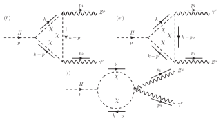
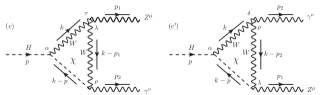
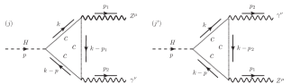
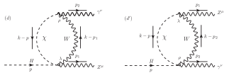
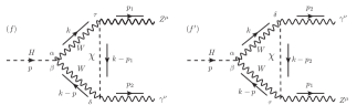
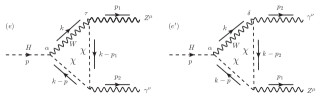
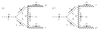
Figure 1: Feynman diagrams of one-loop $W$ boson contributions to $H\rightarrow Z\gamma$ in $R_{\xi}$.

References

- [1] V. M. Abazov et al. [D0], Phys. Lett. B 671 (2009), 349-355.
- [2] S. Chatrchyan et al. [CMS], Phys. Lett. B 726 (2013), 587-609.
- [3] M. Aaboud et al. [ATLAS], JHEP 10 (2017), 112.
- [4] G. Aad et al. [ATLAS], Phys. Lett. B 809 (2020), 135754.
- [5] R. N. Cahn, M. S. Chanowitz and N. Fleishon, Phys. Lett. B 82 (1979), 113-116.
- [6] L. Bergstrom and G. Hulth, Nucl. Phys. B 259 (1985), 137-155.
- [7] R. Martinez, M. A. Perez and J. J. Toscano, Phys. Lett. B 234 (1990), 503-507.
- [8] A. Djouadi, V. Driesen, W. Hollik and A. Kraft, Eur. Phys. J. C 1 (1998) 163.
- [9] A. Djouadi, J. Kalinowski and M. Spira, Comput. Phys. Commun. 108 (1998), 56-74.
- [10] C. W. Chiang and K. Yagyu, Phys. Rev. D 87 (2013) no.3, 033003.
- [11] C. S. Chen, C. Q. Geng, D. Huang and L. H. Tsai, Phys. Rev. D 87 (2013), 075019.
- [12] J. Cao, L. Wu, P. Wu and J. M. Yang, JHEP 09 (2013), 043.
- [13] R. Bonciani, V. Del Duca, H. Frellesvig, J. M. Henn, F. Moriello and V. A. Smirnov, JHEP 08 (2015), 108.
- [14] A. Hammad, S. Khalil and S. Moretti, Phys. Rev. D 92 (2015) no.9, 095008.
- [15] G. Belanger, V. Bizouard and G. Chalons, Phys. Rev. D 89 (2014) no.9, 095023.
- [16] J. M. No and M. Spannowsky, Phys. Rev. D 95 (2017) no.7, 075027.
- [17] S. Taheri Monfared, S. Fayazbakhsh and M. Mohammadi Najafabadi, Phys. Lett. B 762 (2016), 301-308.
- [18] D. Fontes, J. C. Romão and J. P. Silva, JHEP 12 (2014), 043.
- [19] S. Funatsu, H. Hatanaka and Y. Hosotani, Phys. Rev. D 92 (2015) no.11, 115003.
- [20] L. T. Hue, A. B. Arbuzov, T. T. Hong, T. P. Nguyen, D. T. Si and H. N. Long, Eur. Phys. J. C 78 (2018) no.11, 885.
- [21] H. T. Hung, T. T. Hong, H. H. Phuong, H. L. T. Mai and L. T. Hue, Phys. Rev. D 100 (2019) no.7, 075014.
- [22] M. Herrero and R. A. Morales, Phys. Rev. D 102 (2020) no.7, 075040.
- [23] A. Dedes, K. Suxho and L. Trifyllis, JHEP 06 (2019), 115 doi:10.1007/JHEP06(2019)115
- [24] T. Gehrmann, S. Guns and D. Kara, JHEP 09 (2015), 038 doi:10.1007/JHEP09(2015)038
- [25] I. Boradjiev, E. Christova and H. Eberl, Phys. Rev. D 97 (2018) no.7, 073008
- [26] K. H. Phan and D. T. Tran, PTEP 2020 (2020) no.5, 053B08.
- [27] J. C. Pati and A. Salam, Phys. Rev. D 10, 275-289 (1974) [erratum: Phys. Rev. D 11, 703-703 (1975)]
- [28] R. N. Mohapatra and J. C. Pati, Phys. Rev. D 11, 2558 (1975)
- [29] G. Senjanovic and R. N. Mohapatra, Phys. Rev. D 12, 1502 (1975)
- [30] M. Singer, J. W. F. Valle and J. Schechter, Phys. Rev. D 22, 738 (1980)
- [31] J. W. F. Valle and M. Singer, Phys. Rev. D 28, 540 (1983)
- [32] F. Pisano and V. Pleitez, Phys. Rev. D 46, 410-417 (1992)
- [33] P. H. Frampton, Phys. Rev. Lett. 69, 2889-2891 (1992)
- [34] R. A. Diaz, R. Martinez and F. Ochoa, Phys. Rev. D 72, 035018 (2005) [arXiv:hep-ph/0411263 [hep-ph]].
- [35] R. Foot, H. N. Long and T. A. Tran, Phys. Rev. D 50, no.1, R34-R38 (1994) [arXiv:hep-ph/9402243 [hep-ph]].
- [36] S. P. He, Phys. Rev. D 102 (2020) no.7, 075035.
- [37] A. Denner and S. Dittmaier, Nucl. Phys. B 734 (2006) 62.
- [38] H. H. Patel, Comput. Phys. Commun. 197 (2015), 276-290.
- [39] T. Hahn and M. Perez-Victoria, Comput. Phys. Commun. 118 (1999), 153-165.
- [40] W. J. Marciano, C. Zhang and S. Willenbrock, Phys. Rev. D 85 (2012) 013002.
- [41] K. H. Phan and D. T. Tran, [arXiv:2103.10045 [hep-ph]].