On the molecular correlations that result in field-dependent conductivities
in electrolyte solutions

Abstract

Employing recent advances in response theory and nonequilibrium ensemble reweighting, we study the dynamic and static correlations that give rise to an electric field-dependent ionic conductivity in electrolyte solutions. We consider solutions modeled with both implicit and explicit solvents, with different dielectric properties, and at multiple concentrations. Implicit solvent models at low concentrations and small dielectric constants exhibit strongly field-dependent conductivities. We compared these results to the Onsager-Wilson theory of the Wien effect, which provides a qualitatively consistent prediction at low concentrations and high static dielectric constants, but is inconsistent away from these regimes. The origin of the discrepancy is found to be increased ion correlations under these conditions. Explicit solvent effects act to suppress nonlinear responses, yielding a weakly field-dependent conductivity over the range of physically realizable field strengths. By decomposing the relevant time correlation functions, we find that the insensitivity of the conductivity to the field results from the persistent frictional forces on the ions from the solvent. Our findings illustrate the utility of nonequilibrium response theory in rationalizing nonlinear transport behavior.

I Introduction

Due to their ubiquity and importance, electrolyte solutions have been central to the development of theoretical physical chemistry.Harned and Owen (1959) Early research into their structure and dynamics ushered in modern theoretical techniques employing pair distribution functions and linear response theories.Zwanzig (1970); Onsager and Samaras (1934); Onsager and Fuoss (2002); Kubo (1956) Motivated by developments in the theory of systems far from equilibrium and growing experimental capabilities for probing highly nonlinear transport behavior, Gao and Limmer developed a theory of nonlinear response based on a large deviation formalism.Gao and Limmer (2019) Applying this theory to ionic solutions in recent workLesnicki et al. (2020), we demonstrated the ability to employ generalized response relations valid within nonequilibrium steady states together with a nonequilibrium ensemble reweighting scheme to discern the electric field-dependence of the ionic conductivity. In this paper, we examine these relations further, considering models with both implicit and explicit solvent, and comparing our findings to existing analytical theories valid in dilute regimes. We find generally that we are able to estimate the field-dependent conductivity with high accuracy and that its form reflects an interplay between ionic relaxational effects and solvent friction.

Efforts to predict the response of systems far from equilibrium from underlying molecular properties have been stimulated recently in part by a growing body of experimental observations on nanofluidic devices.Bocquet and Charlaix (2010); Bocquet (2020); Kavokine, Netz, and Bocquet (2021) In these systems, nonlinear transport is especially pervasive and often qualitatively sensitive to chemical composition. For example, ionic mobilities have been observed to depend on the driving force of the flow, in a manner dependent on the ion pair and the confining material.Mouterde et al. (2019) Other nonlinear responses, such as ionic rectification, can be achieved in nanofluidic diodes or conical pores.Karnik et al. (2007); He et al. (2009); Picallo et al. (2013); Cheng and Guo (2010) Traditional linear response theory such as Green-Kubo relations are incapable of describing such behaviors due to the breaking of time-reversal symmetry within a steady-state driven by a constant applied field.Zwanzig (1965) Stochastic thermodynamics have offered means of moving beyond equilibrium linear response theory,Seifert (2012) and a number of generalized fluctuation-dissipation relations and bounds have been proposed within its context.Speck and Seifert (2006); Baiesi, Maes, and Wynants (2009); Prost, Joanny, and Parrondo (2009); Dechant and Sasa (2020) Using large deviation theory,Touchette (2018) a nonequilibrium trajectory ensemble framework has been proposed in the context of field driven steady-states for stochastic equations of motion that enables the relationship between fluctuations of time extensive observables in or out of equilibrium to be transparently derived.Gao and Limmer (2017, 2019) Applications to transport and self-assembly have been elucidated in simple systems.Ray and Limmer (2019); Lesnicki et al. (2020); Das and Limmer (2021); GrandPre et al. (2021)

In this work, we extend these efforts to decode the relationship between dynamical fluctuations and response far from equilibrium to systems with full molecular detail in the context of ionic conductivities of electrolyte solutions. To accomplish this, we devise methods of efficiently evaluating the probability of rare dynamical fluctuations through a nonequilibrium ensemble reweighting principle. With access to these probability distributions, we are able to compute averaged observables like the differential conductance and ion pair correlation functions for arbitrary applied fields and concentrations. In what follows, we consider separately models of electrolyte solutions in which the solvent is implicit, allowing us to compare to the Onsager-Wilson continuum theoryWilson (1936) of the Onsager-Wien effect,Onsager and Kim (1957) and those in which the solvent is explicit, allowing us to elucidate the role of ion-water correlations in the conductivity. Snapshots of the systems are shown in Fig. 1. In each section, the theory and numerical methods are first detailed followed by a discussion of the numerical results.

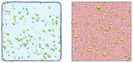
Figure 1: Characteristic snapshots of NaCl solutions from the molecular dynamics simulations with implicit (left) and explicit (right) solvent.

II Implicit Solvent Model

We first consider a model under implicit solvent condition. Specifically, we study a 0.1 M NaCl electrolyte composed of $N_{\mathrm{a}}$ anions and $N_{\mathrm{c}}$ cations with $N=N_{\mathrm{a}}+N_{\mathrm{c}}$ in a volume $V$ and fixed temperature, $T$=300 K. The particles’ positions and velocities are denoted, $\mathbf{r}^{N}=\{\mathbf{r}_{1},\mathbf{r}_{2},\dots,\mathbf{r}_{N}\}$ and $\mathbf{v}^{N}=\{\mathbf{v}_{1},\mathbf{v}_{2},\dots,\mathbf{v}_{N}\}$, respectively. These variables evolve according to an underdamped Langevin equation,

$$\dot{\mathbf{x}}_{i}=\mathbf{v}_{i}\,,\quad m_{i}\dot{\mathbf{v}}_{i}=-\zeta_{i}\mathbf{v}_{i}+\mathbf{F}_{i}\left(\mathbf{r}^{N}\right)+z_{i}\mathbf{E}+\bm{\eta}_{i}$$ (1)

where $m_{i}$ and $z_{i}$ are the $i$th particle’s mass and charge, $\zeta_{i}$ is the friction and $\mathbf{F}_{i}(\mathbf{r}^{N})$ is the interparticle force on the particle $i$. The ions interact through a screened Coulomb potential with dielectric constants $\varepsilon$ = 10 or 60, and Lennard-Jones (LJ) potential. The solutions with low and high values of the dielectric constant we refer to as weak and strong electrolytes, respectively, referring to whether the screening length is comparable or larger than the characteristic ionic size. For pairs $ij$ the total potential $U_{ij}(r)$ is

$$U_{ij}(r)=4\epsilon_{ij}\left[\left(\frac{\sigma_{ij}}{r}\right)^{12}-\left(\frac{\sigma_{ij}}{r}\right)^{6}\right]+\frac{1}{4\pi\varepsilon_{0}\varepsilon}\frac{z_{i}z_{j}}{r}$$ (2)

where $\sigma_{ij}$ and $\epsilon_{ij}$ are the LJ length and energy parameters. To model Na⁺ and Cl^-, we adopt the parameters of Ref. 29. The usual Lorenz-Berthelot combining rules, $\sigma_{ij}=(\sigma_{i}+\sigma_{j})/2$ and $\epsilon_{ij}=(\epsilon_{i}\epsilon_{j})^{1/2}$, were used to calculate the LJ interactions. Each cartesian component of the random force, ${\eta}_{i\alpha}$, obeys Gaussian statistics with mean $\langle{\eta}_{i\alpha}\rangle=0$ and variance $\langle{\eta}_{i\alpha}(t){\eta}_{j\beta}(t^{\prime})\rangle=2k_{\mathrm{B}}T\zeta_{i}\delta_{ij}\delta_{\alpha\beta}\delta(t-t^{\prime})$, where $k_{\mathrm{B}}$ is Boltzmann’s constant. Finally, $\mathbf{E}$ denotes an applied electric field, with magnitude $E$ that drives an ionic current through the periodically replicated system.

In order to reproduce the dynamics of the ions in explicit solvent (see Sec. III), we use the dielectric constant $\varepsilon=60$ of the corresponding water model and the frictions corresponding to the diffusion coefficients calculated for the ions at infinite dilution in the explicit solution: $\zeta_{i}=m_{i}/\tau_{i}$ with relaxation times $\tau_{\mathrm{c}}=10.1$ fs and $\tau_{\mathrm{a}}=21.3$ fs, for the cations and anions with masses $m_{\mathrm{c}}=22.99$ a.m.u. and $m_{\mathrm{a}}=35.45$ a.m.u., respectively. These large frictions effectively render the dynamics overdamped, and we explicitly neglect hydrodynamic effects resulting from integrating out the surrounding solvent flow.Jardat et al. (1999); Ladiges et al. (2021) Simulations are performed for 100 ion pairs, using the LAMMPS codePlimpton (1995); LAM with a modified Langevin thermostat to ensure a Gaussian distribution of the noise. Results for the conductivity are obtained from 10 ns nonequilibrium simulations for finite fields between 0 and 0.1 V/Å, in steps of 0.01 V/Å, with statistical error estimated from bootstrapping, while those for spatial correlations are obtained from 10 independent 10 ns trajectories.

II.1 Nonlinear response from trajectory reweighting

To compute the molar ionic conductivity as a function of the electric field, we employ the formalism of our previous work based on the reweighting of nonequilibrium trajectories. Lesnicki et al. (2020) The differential conductivity $\sigma(E)$ and its molar counterpart $\lambda(E)$ are defined from the derivative of the current with respect to the field,

$$\lambda(E)=\frac{1}{N}V\sigma(E)=\frac{1}{N}\frac{d\langle J\rangle_{E}}{dE}\;,$$ (3)

where given the trajectory, $\mathbf{X}(t_{\mathrm{N}})$, or sequence of positions and velocities over an observation time, $t_{\mathrm{N}}$, the current is given by

$$J[\mathbf{X}(t_{\mathrm{N}})]=\frac{1}{t_{\mathrm{N}}}\int_{0}^{t_{\mathrm{N}}}dt\,j(t)\,,\quad j(t)=\sum_{i=1}^{N}z_{i}v_{i}(t)$$ (4)

a time average of a charge weighted ionic velocity. The $\langle\dots\rangle_{E}$ denotes an average over a trajectory ensemble, where the ions are evolved under the action of an electric field with magnitude $E$. Assuming the fluid is isotropic, the velocity in Eq.  4 is the component in the direction of the applied field. Note that the current $J$ is usually defined in experiments with a factor $1/V$, which explains that with the present notations $d\langle J\rangle_{E}/dE=V\sigma(E)$.

In order to compute Eq. 3 efficiently, we relate the current of a system perturbed by an additional applied field to a system with no applied field. Given the equation of motion in Eq. 1, the probability of observing a trajectory, $\mathbf{X}(t_{\mathrm{N}})$ with an applied field, is

$$P_{\mathbf{E}}[\mathbf{X}(t_{\mathrm{N}})]\propto e^{-\beta U_{\mathbf{E}}[\mathbf{X}(t_{\mathrm{N}})]}$$ (5)

where $\beta=1/k_{B}T$ and for the uncorrelated Gaussian noise, we have an Onsager-Machlup stochastic action of the formKleinert (2009)

$$U_{\mathbf{E}}[\mathbf{X}(t_{\mathrm{N}})] =\sum_{i=1}^{N}\int_{0}^{t_{\mathrm{N}}}dt\frac{\left[m_{i}\dot{\mathbf{v}}_{i}+\zeta_{i}\mathbf{v}_{i}-\mathbf{F}_{i}(\mathbf{r}^{N})-z_{i}\mathbf{E}\right]^{2}}{4\zeta_{i}}\,$$ (6)

where the stochastic calculus is interpreted in the Itô sense. We will consider trajectories in the limit that $t_{\mathrm{N}}$ is large so that only time extensive quantities are relevant.

A perturbing field on the system adds an extra drift to the Gaussian action. As a consequence, we can write the ratio of the probability to observe a trajectory in the presence of the field, denoted as $\mathbf{E}$, relative to no applied field through a Girsanov transformGirsanov (1960)

$$\frac{P_{\mathbf{E}}[\mathbf{X}(t_{\mathrm{N}})]}{P_{\mathbf{0}}[\mathbf{X}(t_{\mathrm{N}})]}=e^{\beta\Delta U_{\mathbf{E}}[\mathbf{X}(t_{\mathrm{N}})]}$$ (7)

where the dimensionless relative action, $\beta\Delta U_{\mathbf{E}}[\mathbf{X}(t_{\mathrm{N}})]$, can be expressed compactly as a sum of three terms, depending on their symmetry under time reversalBasu and Maes (2015)

$$\frac{\Delta U_{\mathbf{E}}}{t_{\mathrm{N}}}=J\frac{E}{2}+Q\frac{E}{2}-N\lambda_{\mathrm{id}}\frac{E^{2}}{4}\,$$ (8)

where for simplicity we take the field along one cartesian direction so that the relative action depends only on its magnitude. The first term is asymmetric under time reversal and identified as the excess entropy production due to the increased nonequilibrium driving. It is given by the product of the total, time averaged current in the direction of the field and the field $E$. The second term in Eq. 8 is symmetric under time reversal and is the product of the field by a quantity referred to as the excess frenesyBaiesi, Maes, and Wynants (2009)

$$Q[\mathbf{X}(t_{\mathrm{N}})] = \frac{1}{t_{\mathrm{N}}}\int_{0}^{t_{\mathrm{N}}}dt\,q(t)$$ (9)

$${\rm with}\ q(t) = \sum_{i=1}^{N}\frac{z_{i}}{\zeta_{i}}\left[m_{i}\dot{v}_{i}(t)-F_{i}(\mathbf{r}^{N})\right]\;,$$

which includes the total time integrated force in the direction of the field weighted by $z_{i}/\zeta_{i}$, and a boundary term resulting in a difference in velocities at times 0 and $t_{\mathrm{N}}$. The remaining term in Eq. 8 is a trajectory independent constant,

$$\lambda_{\mathrm{id}}=\sum_{i=\mathrm{a},\mathrm{c}}\frac{N_{i}}{N}\lambda_{i}=\sum_{i=\mathrm{a},\mathrm{c}}\frac{N_{i}}{N}\frac{D_{i}z_{a}^{2}}{k_{\mathrm{B}}T}$$ (10)

where $D_{i}=k_{\mathrm{B}}T/\zeta_{i}$ is the diffusion coefficient for an isolated ion of type $i$. This constant is the molar Nernst-Einstein conductivity of the solution and is fully determined by the nature of the electrolyte under finite dilutation, i.e. the molar fraction, charge and diffusion coefficients of the independent ions.

With the relative measure between trajectory ensembles defined in Eq. 7, we can relate nonequilibrium trajectory averages in the presence of the field, to equilibrium trajectory averages without the field. For a trajectory observable, $O[\mathbf{X}(t_{\mathrm{N}})]$, this relation is

$$\left\langle O\right\rangle_{E}=\left\langle Oe^{\beta\Delta U_{\mathbf{E}}[\mathbf{X}(t_{\mathrm{N}})]}\right\rangle_{0}$$ (11)

where trajectory averages are over the measure in Eq. 5 with fields $E$ and 0. Setting $O$ to 1, we find a sum rule inherited from the underlying Gaussian process that is quadratic in the field,

$$\left\langle e^{\beta t_{\mathrm{N}}(J[\mathbf{X}(t_{\mathrm{N}})]+Q[\mathbf{X}(t_{\mathrm{N}})])E/2}\right\rangle_{0}=e^{\beta t_{\mathrm{N}}N\lambda_{\mathrm{id}}E^{2}/4}$$ (12)

which is interpretable as the ratio of nonequilibrium to equilibrium trajectory partition functions.

Identifying the joint probability of observing a value of the current and frenesy as $p_{E}(J,Q)=\langle\delta(J-J[\mathbf{X}(t_{\mathrm{N}})],Q-Q[\mathbf{X}(t_{\mathrm{N}})])\rangle_{E}$, we can relate $p_{E}(J,Q)$ to its equilibrium counterpart, using Eq. 11,

$$\frac{\ln p_{0}(J,Q)}{t_{\mathrm{N}}}=\frac{\ln p_{E}(J,Q)}{t_{\mathrm{N}}}-\beta(J+Q)\frac{E}{2}+\beta N\lambda_{\mathrm{id}}\frac{E^{2}}{4}$$ (13)

and thus have a means by which sampling simulations at a variety of finite fields, we are able to reconstruct the joint distribution, $p_{0}(J,Q)$, far into its tails in a manner similar to parallel tempering or replica exchange.Earl and Deem (2005); Sugita, Kitao, and Okamoto (2000) Moreover, with knowledge of the full $p_{0}(J,Q)$, we can in principle compute the molar conductivity $\lambda(E)$ as a continuous function of the applied field. This is done by substituting Eq. 3 into Eq. 11,

$$\lambda(E)=\lim_{t_{\textrm{N}}\rightarrow\infty}\frac{\beta t_{\textrm{N}}}{2N}\left\langle(\delta J^{2}+\delta J\delta Q)e^{\beta\Delta U_{\mathbf{E}}(J,Q)}\right\rangle_{0}$$ (14)

which provides a direct means of evaluating the conductivity. This relation extends the more familiar Einstein-Helfand expressionHelfand (1960); Zwanzig (2001), which is recovered in the absence of the external field.Lesnicki et al. (2020) As we have detailed previously, this route is statistically superior to the explicit estimate afforded from a finite difference approximation to the derivative of the current with applied field. In addition, the above estimator provides information on the conductivity away from points of explicit simulation that is reliable as along as the trajectories ensembles are well overlapping.Frenkel and Smit (2001) We note that as in equilibrium, fluctuation relations like that above can be found for differential quantities, unlike their integral counterparts.Limmer et al. (2013)

II.2 Comparison to Onsager-Wilson theory

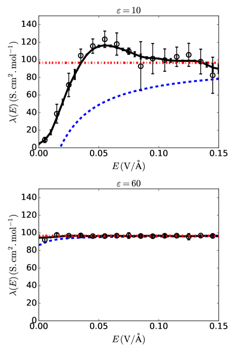
Figure 2: Field-dependent molar ionic conductivities for $\varepsilon=10$ (top panel) and 60 (bottom panel). Black lines are computed from reweighting $p(J,Q)$, and symbols are computed from finite differences of $\left<J\right>_{E}$ versus $E$. Errorbars are one standard deviation of the mean. The red dashed lines correspond to the Nernst-Einstein molar ionic conductivities $\lambda_{\mathrm{id}}$ (Eq. 10). The blue dashed lines correspond to the Wilson molar ionic conductivities considering solely the effect of drag due to the ionic atmosphere (see Eq. 37).

Shown in Fig. 2 are the molar ionic conductivities computed from Eq. 14 continuously as a function of the applied field and from a numerical derivative of the average current versus applied field smoothed with a spline function. In order to apply Eq. 14, we constructed $p_{0}(J,Q)$ with a series of simulations at finite fields at the locations of the direct estimate in Fig. 2, using a generalized version of WHAMKumar et al. (1992) employing the ensemble relation in Eq. 13 to stitch joint histograms of $J$ and $Q$ together. We find quantitative agreement between both estimates, but the calculation employing the ensemble reweighting principle has systematically smaller statistical errors. This is due in part to the avoidance of taking a numerical derivative and in part due to the ability to use information on the conductivity from adjacent fields.

As previously observed,Lesnicki et al. (2020) for the weak electrolyte $\varepsilon=10$, we find a field-dependent conductivity that increases initially quadratically before plateauing at large fields to the Nernst-Einstein limit. At intermediate fields, the weak electrolyte exhibits a slight maxima in ionic molar conductivity. This peak is a consequence of markedly non-Gaussian current fluctuations, with fat tails that are emphasized by the nonequilibrium reweighting at finite field. This behavior is in contrast to that of the strong electrolyte $\varepsilon=60$, which exhibits a nearly field-independent conductivity. The strong electrolyte conductivity is found to saturate to the Nernst-Einstein limiting value for the smallest values of the applied fields considered.

The field-dependent conductivity was considered theoretically by Wilson,Wilson (1936) following foundational work on the linear conductivity by Onsager and Fuoss.Onsager and Fuoss (2002) In his work, Wilson considered a strong electrolyte in the dilute limit, in which the pair correlations are well described by Debye-Hückel theory in the absence of an applied field. From the field-dependence of the pair correlation functions, a force balance on the ions leads to the following expression of the molar conductivityLesnicki et al. (2020)

$$\lambda(E)=\lambda_{\mathrm{id}}+\sum_{i,j=\mathrm{a},\mathrm{c}}\frac{z_{i}}{\zeta_{i}}\int{\rm d}\mathbf{r}\,\bar{\rho}_{j}g^{\prime}_{ij}(r,\theta|E)F_{ij,x}(\mathbf{r})$$ (15)

where $r=|\mathbf{r}|$, $\cos(\theta)=\mathbf{r}\cdot\hat{\mathbf{x}}$ and $g^{\prime}_{ij}(r,\theta|E)=dg_{E}(r,\theta)/dE$ is the derivative of the $ij$ pair distribution function at finite field $E$. The force $F_{ij,x}(\mathbf{r})$ is the component of the pair force in the direction of the field, here assumed to be along the $x$ direction and $\bar{\rho}_{j}=N_{j}/V$.

The Onsager-Wilson predictions are shown in Fig. 2, with the complete expressions for $\lambda(E)$ shown in App. A. In Fig. 2, we have included only the term from ionic relaxation, not the additional electrophoretic terms that result from the counterflow of the solvent (i.e. $\Delta\sigma_{\rm rel}$ but not $\Delta\sigma_{\rm hyd}$ in Eq. 37). This is because in our implicit model, the latter effect is not present. Comparing the theoretical prediction to our numerical results we find poor agreement for the low dielectric system, with Wilson’s theory predicting an unphysical negative conductivity before increasing towards the Nernst-Einstein limit. This failure is due to the break down of the Debye-Hückel approximation, as the low dielectric constant results in a large, nonperturbative interaction between the ions. The agreement is better for the high dielectric system, though the theory predicts a smaller conductivity at zero applied field and a larger response to the field than observed in the simulation.

In order to understand the relationship between our numerical results and Onsager-Wilson theory, we compare the response functions of the pair correlation functions directly. The pair distribution, $g_{\mathrm{a}\mathrm{c}}(r,\theta|E)$, between an anion and a cation can be computed exactly, up to quadrature Hemmer, Holden, and Ratkje (1996); Eu (2010), and its first order correction with applied field is simple. For a symmetric electrolyte, with charges $z=\pm qe$, Onsager’s theory predicts for cations around anions

$$g^{\prime}_{\mathrm{a}\mathrm{c}}(r,\theta|0)= -\cos(\theta)\frac{\beta^{2}z^{3}}{2\pi\varepsilon_{0}\varepsilon\kappa^{2}r^{2}}\times$$

$$\left[\left(1+\kappa r\right)e^{-\kappa r}-\left(1+\frac{\kappa r}{\sqrt{2}}\right)e^{-\kappa r/\sqrt{2}}\right]$$

where $\kappa=\sqrt{4\pi\ell_{\mathrm{B}}\sum_{i=\mathrm{a},\mathrm{c}}\bar{\rho}_{i}q_{i}^{2}}$ is the inverse Debye screening length and $\ell_{\mathrm{B}}=\beta e^{2}/4\pi\varepsilon_{0}\varepsilon$ is the Bjerrum length. The predictions of Onsager theory for the response of the pair distribution functions are shown in Fig. 3 for 0.1M, for both $\varepsilon=60$ ($\kappa^{-1}=8.4~{}\mathrm{\AA}$) and $\varepsilon=10$ ($\kappa^{-1}=3.4~{}\mathrm{\AA}$). The response function is asymmetric, reflecting the polarization of the ionic distribution due to the field. Specifically, there is a build up of cations around anions in the direction of the field and a suppression in the opposite direction. The radial extent of the response is much larger for $\varepsilon=60$ than for $\varepsilon=10$, reflecting the much stronger interactions between the ions (hence smaller $\kappa^{-1}$) in the latter case.

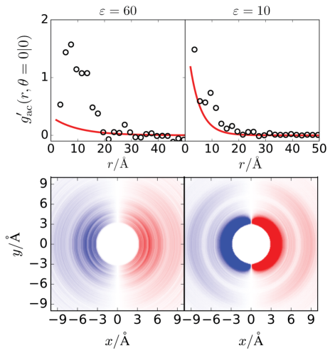
Figure 3: Response of the pair distribution to an applied field for cations around an anion, at equilibrium ($E=0$) for $\varepsilon=60$ (left) and $\varepsilon=10$ (right). Results are shown (top) for Onsager-Wilson theory Eq. II.2 in the solid red line and from simulations using Eq. 19 in the black symbols. Response function, $g_{ac}^{\prime}(x,y|0)$, in the $(x,y)=(r\cos\theta,r\sin\theta)$ plane (bottom) from simulations using Eq. 19. The red (blue) color indicates excess (depletion) of cations in the presence of a field oriented from left to right. The color scale is conserved in both panels but saturates at lower and higher extremes.

The calculation of the response of the ion pair correlation function to an applied electric field within our molecular dynamics simulations is complicated by the use of periodic boundary conditions and finite simulation volumes. The direct calculation from a finite difference of the correlation function evaluated in equilibrium and at small applied field predicts a polarization of the ion distribution erroneously opposite of that predicted by Onsager-Wilson theory. Instead of computing it from an explicit nonequilibrium simulation, we employ a linearized version of Eq. 11 to compute the response function directly within an equilibrium calculation.

Denoting the total configurational distribution at time $t_{\mathrm{N}}$, $\rho_{E}(\mathbf{r}^{N})=\langle\delta[\mathbf{r}^{N}-\mathbf{r}^{N}(t_{\mathrm{N}})]\rangle_{E}$, its form under applied field $E$ relative to its form in equilibrium is given by

$$\rho_{E}(\mathbf{r}^{N})=\rho_{0}(\mathbf{r}^{N})\frac{\langle e^{\beta Et_{\mathrm{N}}(J[\mathbf{X}(t_{\mathrm{N}})]+Q[\mathbf{X}(t_{\mathrm{N}})])/2}\rangle_{0,\mathbf{r}^{N}(t_{\mathrm{N}})}}{\langle e^{\beta Et_{\mathrm{N}}(J[\mathbf{X}(t_{\mathrm{N}})]+Q[\mathbf{X}(t_{\mathrm{N}})])/2}\rangle_{0}}$$ (17)

where we have rewritten the numerator as an equilibrium average conditioned on ending in a particular configuration $\mathbf{r}^{N}(t_{\mathrm{N}})$ at time $t_{\mathrm{N}}$. This form of a nonequilibrium distribution is similar to the Kawasaki distribution.Yamada and Kawasaki (1967); Morriss and Evans (1985); Crooks (2000)

Assuming that the field is small, we can linearize the exponentials to find the first order correction to the configurational distribution. Invoking time-reversal symmetry to move the conditioning to the initial time and a sum rule to eliminate $Q$,Gao and Limmer (2019) we arrive at,

$$\rho_{E}(\mathbf{r}^{N})=\rho_{0}(\mathbf{r}^{N})\left[1-\beta Et_{\mathrm{N}}\langle\delta J\rangle_{0,\mathbf{r}^{N}(0)}\right]+\mathcal{O}(E^{2})$$ (18)

where $\langle\delta J\rangle_{0,\mathbf{r}^{N}(0)}=\langle J\rangle_{0,\mathbf{r}^{N}(0)}-\langle J\rangle_{0}$ is the difference in the time integrated current in the conditioned ensemble with its equilibrium value. This result demonstrates that the correction to the steady state distribution is just the entropy produced upon relaxation from a fixed initial configuration $\mathbf{r}^{N}_{0}$. The average current in equilibrium is zero, but subtracting it out explicitly produces a better estimator for the response function. Specializing to the pair distribution by integrating over all but two ion positions, for one ion of type $i$ and another of type $j$,

$$g^{\prime}_{ij}(r,\theta|0)=\lim_{t_{\textrm{N}}\rightarrow\infty}-\beta g_{ij}(r,\theta|0)t_{\mathrm{N}}\langle\delta J\rangle_{0,r_{ij}(0),\theta_{ij}(0)}$$ (19)

we arrive at a numerically tractable means of computing the change of the ion distribution function from an equilibrium simulation. Namely we correlate an initial density to its transient current. Analogous results have been arrived at through alternative means for computing the Green’s function for the velocity field due to point force in a fluidLesnicki and Vuilleumier (2017) or the mobility profile for a confined fluid.Mangaud and Rotenberg (2020)

We find qualitative similarities to Onsager-Wilson theory, including an accumulation of cations in front of the anion and a depletion at the back of the anion as shown in Fig. 3. However, the magnitudes and characteristic lengthscales are not quantitatively reproduced by the approximate theory, compared in Fig. 3. For both cases, the theory does not correctly predict the magnitude of the response. This is due to the weak coupling approximation used in Onsager-Wilson theory that is valid only in the limit of small $\kappa$ and weak ion correlations. This is manifested in the qualitatively inaccurate prediction of the field-dependent conductivity for the weak electrolyte, and a stronger field-dependence than observed in the strong electrolyte. In the low dielectric solution, ions interact strongly and are much more responsive to the field in both the simulation and the theory. The ionic relaxation effect decreases the conductivity from the Nernst-Einstein value, and its overprediction is the cause of the spurious negative conductivity predicted in Fig. 2.

III Explicit Solvent Model

We next consider a model with explicit solvent conditions. Specifically, we study a NaCl electrolyte composed of $N_{\mathrm{a}}$ anions, $N_{\mathrm{c}}$ cations and $N_{\mathrm{w}}$ water molecules in a volume $V$ and fixed temperature $T=300$K. We will consider two concentrations of ions, 0.1 M and 1.0 M. As before, the species’ positions and velocities are denoted, $\mathbf{r}^{N}=\{\mathbf{r}_{1},\mathbf{r}_{2},\dots,\mathbf{r}_{N}\}$ and $\mathbf{v}^{N}=\{\mathbf{v}_{1},\mathbf{v}_{2},\dots,\mathbf{v}_{N}\}$, respectively. These variables evolve according to the same underdamped Langevin equation as in Eq. 1. The relaxation time $\tau=1000$ fs is used for all species. The pairwise interaction potential $U_{ij}(r)$ consists of LJ and electrostatic terms such that

$$U_{ij}(r)=4\epsilon_{ij}\left[\left(\frac{\sigma_{ij}}{r}\right)^{12}-\left(\frac{\sigma_{ij}}{r}\right)^{6}\right]+\frac{1}{4\pi\varepsilon_{0}}\frac{z_{i}z_{j}}{r}$$ (20)

where $z_{i}$ and $z_{j}$ are the charges on sites $i$ and $j$, $r_{ij}$ is the site-site separation, $\sigma_{ij}$ and $\epsilon_{ij}$ are the length and energy parameters, and $\epsilon_{0}$ is the permittivity of free space. The LJ parameters for Na⁺ and Cl^- are chosen the same as in the implicit model, while the water molecules are modeled with the flexible q-TIP4P/F model Habershon, Markland, and Manolopoulos (2009). The usual Lorenz-Berthelot combining rules, $\sigma_{ij}=(\sigma_{i}+\sigma_{j})/2$ and $\epsilon_{ij}=(\epsilon_{i}\epsilon_{j})^{1/2}$, were used to calculate the LJ interactions. Simulations are performed for 100 ion pairs and 55508 (5540) water molecules for the 0.1M (1M) solution, using the LAMMPS codePlimpton (1995); LAM with a modified Langevin thermostat to ensure a Gaussian distribution of the noise. Results for the conductivity are obtained from a series of 1 ns nonequilibrium simulations for finite field between 0 and 0.1 V/Å, in steps of 0.01 V/Å, with statistical error estimated from bootstrapping, while those for temporal correlations are obtained from 10 independent 10 ns trajectories.

III.1 Trajectory reweighting of multicomponent systems

As in the implicit model, the stochastic action can be constructed by comparing the ratio of the probability to observe a trajectory with and without a perturbing field. The flexible water model employed allows for independent noises to act on each atom in the water molecule, while a rigid model would color the noise due to the imposed geometric constraint. For generality and for utility in subsequent analysis, we consider different perturbing fields with magnitudes, $\mathbf{E}=\{{E}_{\textrm{i}},{E}_{\textrm{w}}\}$ for the ions and water, respectively. As before, we take the field along one cartesian direction so that the relative action depends only on these magnitudes. We further introduce the notation $\mathbf{E^{(2)}}=\{{E}_{\textrm{i}}^{2},{E}_{\textrm{w}}^{2}\}$. The stochastic action, decomposed according to symmetry under time reversal, is then

$$\frac{\Delta U_{\mathbf{E}}}{t_{N}}=\frac{1}{2}[\mathbf{J}+\mathbf{Q}]\cdot\mathbf{E}-\frac{1}{4}\bm{N\lambda}\cdot\mathbf{E}^{(2)}$$ (21)

which now depends on components of the currents, $\mathbf{J}=\{J_{\textrm{i}},J_{\textrm{w}}\}$, and excess frenesy, $\mathbf{Q}=\{Q_{\textrm{i}},Q_{\textrm{w}}\}$, and vector $\bm{N\lambda}=\{N_{\mathrm{a}}\lambda_{\mathrm{a}}+N_{\mathrm{c}}\lambda_{\mathrm{c}},N_{\mathrm{w}}\lambda_{\mathrm{w}}\}$ from the ions and the water, respectively. The definitions of the dynamical variables are the same as in the implicit model, where sums are interpreted atom-wise over the specified group. Specifically for group $\alpha=\{\mathrm{i},\mathrm{w}\}$, the associated current is

$$J_{\alpha}[\mathbf{X}(t_{\mathrm{N}})] =\frac{1}{t_{\mathrm{N}}}\int_{0}^{t_{\mathrm{N}}}dt\,j_{\alpha}(t)\,,\quad j_{\alpha}(t)=\sum_{i\in N_{\alpha}}z_{i}v_{i}(t)$$ (22)

and frenesy,

$$Q_{\alpha}[\mathbf{X}(t_{\mathrm{N}})] = \frac{1}{t_{\mathrm{N}}}\int_{0}^{t_{\mathrm{N}}}dt\,q_{\alpha}(t)$$ (23)

$$q_{\alpha}(t) = \sum_{i\in N_{\alpha}}\frac{z_{i}}{\zeta_{i}}\left[m_{i}\dot{v}_{i}(t)-F_{i}(\mathbf{r}^{N})\right]$$

The constant $\lambda_{\mathrm{w}}$ introduced above in $\bm{N\lambda}$ is defined for ions as in Eq. 10, with a sum over oxygen and hydrogen atoms, but it no longer has the interpretation of a contribution to the molar Nernst-Einstein conductivity. While the waters are flexible, they are not dissociable, and their motion is described by a center of mass motion, with additional rotational and vibrational modes. The charge neutrality of the water molecule dictates that its center of mass motion does not contribute to the ionic current, however rotational and vibrational motions may, transiently.

With the relative measure between trajectory ensembles defined in Eq. 7, we can relate nonequilibrium trajectory averages in the presence of the field, to equilibrium trajectory averages without the field. Following our previous workLesnicki et al. (2020), an average of an arbitrary observable $\mathcal{O}$ under an applied field can be expressed as

$$\left\langle\mathcal{O}\right\rangle_{E}=\frac{\left\langle\mathcal{O}e^{\frac{\beta t_{\mathrm{N}}}{2}(\mathbf{J}+\mathbf{Q})\cdot\mathbf{E}}\right\rangle_{0}}{\left\langle e^{\frac{\beta t_{\mathrm{N}}}{2}(\mathbf{J}+\mathbf{Q})\cdot\mathbf{E}}\right\rangle_{0}}$$ (24)

a weighted sum in the absence of the field. The average is over a joint equilibrium distribution that can be obtained by reweighting its nonequilibrium counterpart $p_{E}(\mathbf{J},\mathbf{Q})=\langle\delta(J_{\textrm{i}}-J_{\textrm{i}}[\mathbf{X}(t_{\mathrm{N}})],Q_{\textrm{i}}-Q_{\textrm{i}}[\mathbf{X}(t_{\mathrm{N}})],J_{\textrm{w}}-J_{\textrm{w}}[\mathbf{X}(t_{\mathrm{N}})],Q_{\textrm{w}}-Q_{\textrm{w}}[\mathbf{X}(t_{\mathrm{N}})])\rangle_{E}$ according to the equation

$$\frac{\ln p_{0}(\mathbf{J},\mathbf{Q})}{t_{\mathrm{N}}}=\frac{\ln p_{E}(\mathbf{J},\mathbf{Q})}{t_{\mathrm{N}}}-\beta(\mathbf{J}+\mathbf{Q})\cdot\frac{\mathbf{E}}{2}+\frac{\beta}{4}\bm{N\lambda}\cdot\mathbf{E}^{(2)}$$ (25)

as before. Note that in Eq. 24, the dynamical quantities of the water are coupled with the ions through the relative action. Even for observables that depend only on a subset of degrees of freedom, like those of the ions, the exponential bias correlates them with the entire set of degrees of freedom in the system.

A practical difficulty arises in applying Eq. 25 straightforwardly. As $\mathbf{J}$ and $\mathbf{Q}$ are both extensive variables in particle number and observation time, when both are large, $p_{E}(\mathbf{J},\mathbf{Q})$ becomes exponentially peaked about its most typical values, and the reweighting factors become large enough that it is difficult to represent them numerically. This makes performing the reweighting cumbersome. A solution is found for observables that depend only on the ion degrees of freedom, by treating the contribution to the reweighting factor from the water approximately. An accurate approximation can be found by first writing the joint distribution using Bayes theorem,

$$p_{E}(\mathbf{J},\mathbf{Q}) = p_{E}(J_{\textrm{i}},Q_{\textrm{i}}|J_{\textrm{w}},Q_{\textrm{w}})p_{E}(J_{\textrm{w}},Q_{\textrm{w}})$$

$$= p_{E}(J_{\textrm{i}},Q_{\textrm{i}}|J_{\textrm{w}},Q_{\textrm{w}})\exp[-N_{\mathrm{w}}t_{\mathrm{N}}I_{E}(\bar{j}_{\textrm{w}},\bar{q\vphantom{j}}_{\textrm{w}})]$$

where the first term on the right hand side is a conditional probability, and in the second line $I_{E}(\bar{j}_{\textrm{w}},\bar{q\vphantom{j}}_{\textrm{w}})$ is the rate function for intensive variables $\bar{j}_{\mathrm{w}}=J_{\textrm{w}}/N_{\mathrm{w}}$ and $\bar{q\vphantom{j}}_{\textrm{w}}=Q_{\textrm{w}}/N_{\mathrm{w}}$. The form of the marginal distribution of the water variables is known as a large deviation form, and holds in the limit of large number of particles and observation time. Under the assumption that the joint distribution $I_{E}(\bar{j}_{\textrm{w}},\bar{q\vphantom{j}}_{\textrm{w}})$ is peaked in $(\bar{j}_{\textrm{w}},\bar{q\vphantom{j}}_{\textrm{w}})$, we use a saddle point approximation to evaluate their contribution to the reweighting factors in Eq. 24. For the marginal distribution of the ion variables $p_{0}(J_{\mathrm{i}},Q_{\mathrm{i}})$ this leads to an approximate reweighting,

$$\ln p_{0}(J_{\mathrm{i}},Q_{\mathrm{i}}) \approx\ln p_{E}[J_{\mathrm{i}},Q_{\mathrm{i}}|j_{\textrm{w}}^{*}(E_{\textrm{w}}),q_{\textrm{w}}^{*}(E_{\textrm{w}})]$$ (27)

$$-\beta t_{\mathrm{N}}(J_{\mathrm{i}}+Q_{\mathrm{i}})\frac{{E}_{\mathrm{i}}}{2}-\mathcal{N}(E_{\mathrm{i}},E_{\mathrm{w}})$$

where $[j_{\textrm{w}}^{*}(E),q_{\textrm{w}}^{*}(E)]$ denotes the maximizer

$$[j_{\textrm{w}}^{*}(E),q_{\textrm{w}}^{*}(E)]=\underset{(\bar{j}_{\textrm{w}},\bar{q\vphantom{j}}_{\textrm{w}})}{\textrm{argmin}}\left\{\,I_{E}(\bar{j}_{\textrm{w}},\bar{q\vphantom{j}}_{\textrm{w}})+\beta(\bar{j}_{\textrm{w}}+\bar{q\vphantom{j}}_{\textrm{w}})E/2\right\}$$ (28)

and the normalization constant $\mathcal{N}(E_{\mathrm{i}},E_{\mathrm{w}})$ becomes

$$\mathcal{N}=N_{\mathrm{w}}t_{\mathrm{N}}I_{E_{\textrm{w}}}(j^{*}_{\textrm{w}},q^{*}_{\textrm{w}})+\frac{\beta}{2}N_{\mathrm{w}}t_{\mathrm{N}}(j^{*}_{\textrm{w}}+q^{*}_{\textrm{w}})E_{\textrm{w}}-\frac{\beta}{4}t_{\mathrm{N}}\bm{N\lambda}\cdot\mathbf{E}^{(2)}$$ (29)

which depends only on the applied external fields, not on any fluctuating variables.

We use this approximate expression for the reweighting procedure in the results presented below. As the extensive dynamical variables related to water molecules are usually larger in magnitude compared to the ions by an order of magnitude, due to $N_{\mathrm{w}}\gg N_{\mathrm{i}}$, this expression greatly reduces numerical issues in dealing with the exponential of very large numbers. Note that when the rate function $I_{E}(\bar{j}_{\textrm{w}},\bar{q\vphantom{j}}_{\textrm{w}})$ is quadratic, or the ions and water are uncorrelated, this approximation is exact. Outside of those regimes, we still find it admits a faithful approximation to the exact reweighting relation in Eq. 25, especially when using additional fields to reconstruct $\ln p_{0}(J_{\mathrm{i}},Q_{\mathrm{i}})$ far into the tails of the distribution.

To compute the molar ionic conductivity, we can straightforwardly adapt Eq. 14. We first consider the physical condition where the same field $E_{\textrm{i}}=E_{\textrm{w}}=E$ is applied on the whole system. The ionic conductivity defined as $\lambda(E)=(1/N_{\textrm{i}})d\langle J_{\textrm{i}}\rangle_{E}/dE$ can be computed as

$$\lambda(E)= \lim_{t_{\textrm{N}}\rightarrow\infty}\frac{\beta t_{\textrm{N}}}{2N_{\textrm{i}}}\left\langle(\delta J_{\textrm{i}}^{2}+\delta J_{\textrm{i}}\delta Q_{\textrm{i}}+\delta J_{\textrm{i}}\delta J_{\textrm{w}}\right.$$ (30)

$$\left.+\delta J_{\textrm{i}}\delta Q_{\textrm{w}})e^{\beta\Delta U_{\mathbf{E}}[\mathbf{X}(t_{\mathrm{N}})]}\right\rangle_{0}$$

which includes both the self-correlations among the ions, and the cross-correlations between ions and water molecules. This becomes evident upon a Taylor expansion on Eq. 30 to second order in the applied field, where the long time limit is implied but suppressed for brevity,

$$\lambda(E)=\frac{\beta t_{\mathrm{N}}}{2N_{\textrm{i}}}\left(\left\langle J_{\textrm{i}}^{2}\right\rangle_{0}+\left\langle J_{\textrm{i}}J_{\textrm{w}}\right\rangle_{0}\right)$$ (31)

$$+\frac{3\beta^{3}t_{\mathrm{N}}^{3}}{8N_{\textrm{i}}}\left(\frac{1}{6}\left\langle J_{\textrm{i}}^{4}\right\rangle_{0}-\frac{1}{2}\left\langle J_{\textrm{i}}^{2}\right\rangle_{0}^{2}+\frac{1}{2}\left\langle\delta(J_{\textrm{i}}^{2})\delta(Q_{\textrm{i}}^{2})\right\rangle_{0}\right.$$

$$+\frac{1}{2}\left\langle J_{\textrm{i}}^{3}J_{\textrm{w}}\right\rangle_{0}-\frac{3}{2}\left\langle J_{\textrm{i}}J_{\textrm{w}}\right\rangle_{0}\left\langle J_{\textrm{i}}^{2}\right\rangle_{0}+\left\langle\delta(J_{\textrm{i}}^{2})\delta(Q_{\textrm{i}}Q_{\textrm{w}})\right\rangle_{0}$$

$$+\frac{1}{2}\left\langle\delta(J_{\textrm{i}}J_{\textrm{w}})\delta(Q_{\textrm{i}}^{2})\right\rangle_{0}+\frac{1}{2}\left\langle\delta(J_{\textrm{i}}^{2})\delta(J_{\textrm{w}}^{2}))\right\rangle_{0}-\left\langle J_{\textrm{i}}J_{\textrm{w}}\right\rangle_{0}^{2}$$

$$+\frac{1}{2}\left\langle\delta(J_{\textrm{i}}^{2})\delta(Q_{\textrm{w}}^{2})\right\rangle_{0}+\left\langle\delta(J_{\textrm{i}}J_{\textrm{w}})\delta(Q_{\textrm{i}}Q_{\textrm{w}})\right\rangle_{0}+\frac{1}{6}\left\langle J_{\textrm{i}}J_{\textrm{w}}^{3}\right\rangle_{0}$$

$$\left.-\frac{1}{2}\left\langle J_{\textrm{i}}J_{\textrm{w}}\right\rangle_{0}\left\langle J_{\textrm{i}}^{2}\right\rangle_{0}+\frac{1}{2}\left\langle\delta(J_{\textrm{i}}J_{\textrm{w}})\delta(Q_{\textrm{w}}^{2})\right\rangle_{0}\right)E^{2}+O(E^{4})$$

where time-reversal and spatial symmetry are invoked to eliminate terms of zero value.

Alternatively, one can construct an artificial perturbation where $E_{\mathrm{i}}=E$ and $E_{\mathrm{w}}=0$, where the external field is only applied to the ions. While this condition is not physical, its utility is illustrated in the expression for molar ionic conductivity,

$$\tilde{\lambda}(E_{i})=\lim_{t_{\textrm{N}}\rightarrow\infty}\frac{\beta t_{\textrm{N}}}{2N_{\textrm{i}}}\left\langle(\delta J_{\textrm{i}}^{2}+\delta J_{\textrm{i}}\delta Q_{\textrm{i}})e^{\beta\Delta U_{\mathbf{E}_{i}}[\mathbf{X}(t_{\mathrm{N}})]}\right\rangle_{0}$$ (32)

where compared to Eq. 30, all the cross-correlations between the ions and the water disappear in the Taylor expansion, where again the long time limit is implied

$$\tilde{\lambda}(E_{i}) =\frac{\beta t_{\mathrm{N}}}{2N_{\textrm{i}}}\left\langle J_{\textrm{i}}^{2}\right\rangle_{0}+\frac{3\beta^{3}t_{\mathrm{N}}^{3}}{8N_{\textrm{i}}}\left(\frac{1}{6}\left\langle J_{\textrm{i}}^{4}\right\rangle_{0}-\frac{1}{2}\left\langle J_{\textrm{i}}^{2}\right\rangle_{0}^{2}\right.$$ (33)

$$+\left.\frac{1}{2}\left\langle\delta(J_{\textrm{i}}^{2})\delta(Q_{\textrm{i}}^{2})\right\rangle_{0}\right)E_{i}^{2}+O(E_{i}^{4})$$

Thus by comparing the conductivity under the two scenarios, we can obtain an estimate of the contribution from ion-water correlations, which is not readily extracted from direct simulations and integrations of correlations functions.

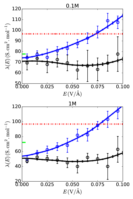
Figure 4: Field-dependent conductivities of the explicit model where an external field is applied on both the ions and water (black), and only applied on the ions (blue). The lines are computed from the reweighting method, while the symbols are computed from finite differences of $\left\langle J_{\textrm{i}}\right\rangle_{E}$ versus $E$, with one standard deviation as errorbars. The top are computed at 0.1 M and bottom 1.0 M. Green tick marks on the left axis denote the MSA prediction for $E=0$.

III.2 Ion-water correlations suppress nonlinear response

Shown in Fig. 4 are the field-dependent conductivities of the explicit solvent system at two concentrations, 0.1M and 1M. The reweighted results for both are computed from Eq. 27 using $t_{\mathrm{N}}=10\textrm{fs}$, which is long enough to justify the saddle point approximation and converge the mean reweighted current. Specifically, we first constructed $p_{0}(J_{\textrm{i}},Q_{\textrm{i}})$ using a series of simulations at finite fields at the locations of the direct estimate in Fig. 4, and the generalized version of WHAM to stitch joint histograms of $J_{\textrm{i}}$ and $Q_{\textrm{i}}$ together. Additionally, we have computed the conductivity from a numerical derivative of the average current directly from a set of simulations at fixed field. While the two estimates are in good quantitative agreement, the statistical errors are much smaller for the reweighted results, as data across the whole fields are supplemented in each estimate.

We find the conductivity is only weakly dependent on the field and the curve is well fitted by a polynomial with a positive fourth order and a negative second order term. The curves for the two different concentrations, 0.1M and 1M are remarkably similar, though the latter exhibits a consistently lower conductivity. The conductivity at zero field for both concentrations is suppressed relative to its value at infinite dilution, or compared to its implicit solvent value. For 0.1M, the ionic molar conductivity at zero field agrees well with the result from the mean spherical approximation (MSA, see App. B),Dufrêche et al. (2005) which is equal to 78 S cm${}^{2}/$mol using ionic radii $r_{\textrm{c}}=3.05$Å and $r_{\textrm{a}}=3.62$Å ). This agreement implies that at 0.1M, the dynamical response of the ions is well described by Gaussian fluctuations in the density and velocity fields.Chandler (1993); Speck (2013) More details are available in App. B. MSA however overpredicts the conductivity at 1.0 M with a value of 72 S cm${}^{2}/$mol, reflecting the underestimation of ionic correlation effects. At unphysically high fields, there is a significant nonlinear response due to the dielectric saturation of the solvent, see App. C.

From the ensemble reweighting theory presented in the previous section, we have a means of decoupling the contributions to the field-dependent conductivity from the solvent and those from the ions. Specifically, we can use a generalized ensemble where only a field is applied to the ions, not the water, to deduce which correlations suppress the field-dependence that result directly from the water. When the field is only applied on the ions for both concentrations, the conductivity grows quadratically with a large positive second order term. This is shown in Fig. 4. The drastic difference between these two sets of results can be unravelled by a comparison between the generalized fluctuation-dissipation relationships in Eq. 31 and Eq. 33, where all cross-correlations between the ions and water are absent from the latter expression. More specifically, the lower conductivity at zero field when the field is applied on both the ions and water is a direct result of negative correlations in $\left\langle J_{\textrm{i}}J_{\textrm{w}}\right\rangle_{0}$ at equilibrium. The negative second order coefficient results from the negative fourth order correlations between ions and water, among which the dominant term is $\left\langle\delta(J_{\textrm{i}}^{2})\delta(Q_{\textrm{w}}^{2})\right\rangle_{0}$ due to the larger number of water molecules and subsequently larger fluctuations in $Q_{\textrm{w}}$.

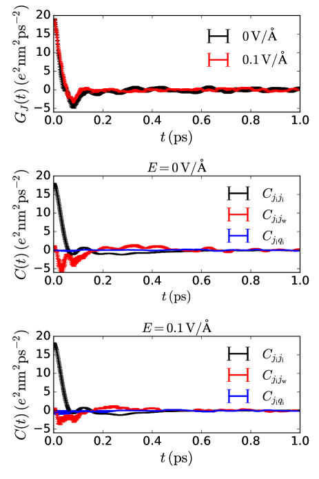
Figure 5: Time correlation functions for field-dependent conductivities of 0.1 M explicit solvent solution. (Top) time correlation functions $G_{J}(t)=C_{j_{\textrm{i}}j_{\textrm{i}}}(t)+C_{j_{\textrm{i}}j_{\textrm{w}}}(t)$ for $E=0$ and $E=0.1\,$V$/\mathrm{\AA}$. (Middle) Contributions to the conductivity from current-current and current-frenesy for $E=0\,$V$/\mathrm{\AA}$. (Bottom) Contributions to the conductivity from current-current and current-frenesy for $E=0.1\,$V$/\mathrm{\AA}$. Throughout errorbars are one standard deviation from the mean.

To gain more physical insight into the relevant correlations, we rewrite the equation for the conductivity using time integrated correlation functions

$$\lambda(E) =\lim_{t_{\mathrm{N}}\rightarrow\infty}\frac{\beta t_{\mathrm{N}}}{2N_{\textrm{i}}}\left\langle\delta J_{\textrm{i}}^{2}+\delta J_{\textrm{i}}\delta J_{\textrm{w}}+\delta J_{\textrm{i}}\delta Q_{\textrm{i}}+\delta J_{\textrm{i}}\delta Q_{\textrm{w}}\right\rangle_{E}$$ (34)

$$=\frac{\beta}{N_{\textrm{i}}}\int_{0}^{\infty}dt\,\,\left[G_{J}(t)+G_{Q}(t)\right]$$

where $G_{J}(t)=C_{j_{\textrm{i}}j_{\textrm{i}}}(t)+C_{j_{\textrm{i}}j_{\textrm{w}}}(t)$, with

$$C_{j_{\textrm{i}}j_{\textrm{i}}}(t) =\left\langle\delta j_{\textrm{i}}(0)\delta j_{\textrm{i}}(t)\right\rangle_{E}$$ (35)

$$C_{j_{\textrm{i}}j_{\textrm{w}}}(t) =\frac{1}{2}\left\langle\delta j_{\textrm{i}}(0)\delta j_{\textrm{w}}(t)+\delta j_{\textrm{i}}(0)\delta j_{\textrm{w}}(-t)\right\rangle_{E}$$

and $G_{Q}(t)=C_{j_{\textrm{i}}q_{\textrm{i}}}(t)+C_{j_{\textrm{i}}q_{\textrm{w}}}(t)$, with

$$C_{j_{\textrm{i}}q_{\textrm{i}}}(t) =\frac{1}{2}\left\langle\delta j_{\textrm{i}}(0)\delta q_{\textrm{i}}(t)+\delta j_{\textrm{i}}(0)\delta q_{\textrm{i}}(-t)\right\rangle_{E}$$ (36)

$$C_{j_{\textrm{i}}q_{\textrm{w}}}(t) =\frac{1}{2}\left\langle\delta j_{\textrm{i}}(0)\delta q_{\textrm{w}}(t)+\delta j_{\textrm{i}}(0)\delta q_{\textrm{w}}(-t)\right\rangle_{E}$$

The conductivity away from equilibrium is a sum of the integrated current-current correlation function, denoted by $G_{J}$, and integrated current-frenesy correlation function, denoted by $G_{Q}$. At zero field, $G_{Q}$ is zero due to time reversal symmetry, leaving $G_{J}$ as the only contribution to the zero-field conductivity. At finite fields when $G_{Q}$ should contribute to the conductivity as well, for the concentrations studied, we find that the contribution from $C_{j_{\textrm{i}}q_{\textrm{i}}}(t)$ is negligible compared to the other three terms. This is due to the screening effect of the explicit water molecules that results in the ions being largely dissociated, so that the effect of ion-ion interactions arises mainly from the relaxation of the ionic cloud rather than from ion pairing and is thus weaker than short-range ion-water interactions. The $C_{j_{\textrm{i}}q_{\textrm{w}}}(t)$ term exhibits large statistical fluctuations due to the larger number and stronger intramolecular forces of the water molecules, and is thus much more difficult to converge by brute force calculations. We have to infer its contribution from the measured conductivities using the generalized fluctuation-dissipation relationships.

Figure 5 shows the current-current contribution to the response function for the 0.1M explicit system at equilibrium $E=0$ and at a finite field $E=0.1\mathrm{V/\AA}$. Also in Fig. 5, the total correlation function for $E=0$ and $E=0.1\mathrm{V/\AA}$ are decomposed into their various pieces. At zero field, both the ion-ion current self-correlation and the ion-water current cross-correlation exhibit noticeable recoil effects evident in transient negative correlations. The former (ion-ion), which spreads over longer timescales, integrates to a positive contribution, and is the only term responsible for the zero-field conductivity when the field is only applied to the ions. The latter (ion-water) integrates to a much smaller negative contribution, which accounts for the difference between the zero-field conductivities between the two sets in Fig. 4. At a higher field $E=0.1~{}\mathrm{V/\AA}$, the recoil effect in both correlations is reduced, resulting in a larger integrated value of both current-current correlation functions, and a more positive $G_{J}(t)$.

We can infer the large contribution from $C_{j_{\textrm{i}}q_{\textrm{w}}}(t)$ at finite field by contrasting the behavior of $\lambda(E)$ and $\tilde{\lambda}(E)$. In the case where the field is applied only on the ions, the correlation function $C_{j_{\textrm{i}}j_{\textrm{i}}}(t)$ integrates to a similarly large contribution as in the case when the field is applied to both ions and water, and one that is larger than its zero field value. As $C_{j_{\textrm{i}}j_{\textrm{w}}}(t)$ and $C_{j_{\textrm{i}}q_{\textrm{i}}}(t)$ are persistently small at $E=0.1\mathrm{V/\AA}$, the large difference difference between $\lambda(E)$ and $\tilde{\lambda}(E)$ must result from significant negative contributions in the current-frenesy correlation function $C_{j_{\textrm{i}}q_{\textrm{w}}}(t)$ between the ions and the water. The physical origin of this negative correlation is the relaxation effects that result from ion displacements that transiently distort the local dielectric environment and generate a restoring force on the water molecules from the compensating ionic cloud left behind. This term dominates the total correlation function and compensates the increase in the current-current correlation functions, yielding a weak dependence on field of the conductivity. Thus while the current-frenesy correlation function is difficult to compute explicitly, from the above analysis we are able to infer its effect using the decomposition of time correlation functions.

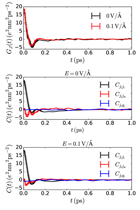
Figure 6: Time correlation functions for field-dependent conductivities of 1.0 M explicit solvent solution. (Top) time correlation functions $G_{J}(t)=C_{j_{\textrm{i}}j_{\textrm{i}}}(t)+C_{j_{\textrm{i}}j_{\textrm{w}}}(t)$ for $E=0$ and $E=0.1\,$V$/\mathrm{\AA}$. (Middle) Contributions to the conductivity from current-current and current-frenesy for $E=0\,$V$/\mathrm{\AA}$. (Bottom) Contributions to the conductivity from current-current and current-frenesy for $E=0.1\,$V$/\mathrm{\AA}$. Throughout errorbars are one standard deviation from the mean.

Figure  6 shows the correlation functions for the 1.0 M system. Qualitatively, they are very similar to those for the 0.1 M solution. Both systems exhibit noticeable recoil effects in the current-current function due to ion-ion terms. In the 1.0 M solution, the transient negative correlation is larger than in the 0.1 M solution. This is also true for the current-current function due to ion-water terms. The combination of these negative correlations results in the reduced conductivity at $E=0~{}\mathrm{V/\AA}$. As for the small concentration, the currrent-frenesy correlations from ion-ion terms are negligible even at 0.1 V/$\mathrm{\AA}$, and the suppressed field-dependence results from the currrent-frenesy correlations from ion-water terms.

IV Comparison between implicit and explicit solvents

The ability to efficiently compute field-dependent conductivities generally enables a comparison between different solvent representations. Comparing the implicit and explicit models, we find that at the same concentration of 0.1 M the conductivity in the implicit model is higher by nearly 30 %. The implicit model has been parameterized to yield the correct limiting conductivity in the infinite dilution regime, so the enhanced conductivity in the implicit model at zero applied field results from an inaccurate description of ion-ion correlations. It is well known that inter-ionic correlations are not accurately described by screening by a lone dielectric constant, as explicit solvent models induce potentials of mean force between ions that exhibit significant structure.Pettitt and Rossky (1986) Additionally, in our study only the explicit model considers hydrodynamic effects that result from momentum transfer and counter flows around the ion. When we neglect hydrodynamic effects for the implicit solvent, we find consistent agreement between Onsager’s theory and MSA for the strong electrolyte. Indeed, in the dilute limit MSA reduces to Wilson’s theory. However, neither linear theory is capable of describing the weak electrolyte, as both MSA and Onsager’s theory erroneously predict a negative conductivity. MSA is capable of qualitatively predicting the reduced conductivity with concentration for the strong electrolyte, but is not quantitatively accurate.

With application of an electric field, we find that both the implicit and explicit models have a nearly constant conductivity for this strong electrolyte system, but for different reasons. The implicit model saturates its conductivity to the Nernst-Einstein value at zero field. Increasing the field has little effect on the already weak ion correlations. The nearly constant conductivity in the explicit model, however, results from a balancing of decreased inter-ionic correlations that act to increase the conductivity with increased ion-water correlations that suppress it. In other models, there is no reason that these need to be so carefully balanced, suggesting that care should be taken in interpreting results of implicit models under large applied fields.

V Conclusion

We have shown how to relate dynamical fluctuations of molecular quantities within nonequilibrium steady states to observable macroscopic response for detailed molecular models of electrolyte solutions. Such calculations are made possible formally by advances in the theory of nonequilibrium steady statesGao and Limmer (2019) and numerically by employing an ensemble reweighting relation that enables an importance sampling of a probability distribution of time integrated functions.Lesnicki et al. (2020) Considering the field-dependence of the ionic conductivity, we have shown how nonlinear relationships between an ionic current and applied electric field can emerge in weak electrolytes as ion correlations are reduced, and how they are mitigated in strong electrolytes due to persistent solvent friction. Whereas for strong electrolytes at low concentrations, existing approximate theoriesWilson (1936); Dufrêche et al. (2005) can accurately predict the conductivity and its field-dependence, for weak electrolytes or elevated concentrations these theories break down.

In the explicit solvent case, the present theoretical and numerical techniques also provide new opportunities to investigate coupled charge and mass transport in electrolytesSedlmeier et al. (2014) or the origin of the frequency-dependent solvent friction on the ions and its consequences on the conductivity of electrolyte solutions.Chandra and Bagchi (2000); Dufrêche et al. (2002); Balos et al. (2020) The present approach with explicit solvent can also be used to test theories beyond the hypotheses underlying that of Onsager and Wilson, such as based on lattice models,Eyink, Lebowitz, and Spohn (1996) fluctuating hydrodynamicsPéraud et al. (2017); Donev et al. (2019) or stochastic density functional theory.Démery and Dean (2016) While we have considered bulk solutions of monovalent electrolytes, our approach is straightforwardly applied for multivalent ions, where nonlinear responses due to field-induced ion pair dissociation should be more prominent, and can be extended to instances of transport in confinement,Pean et al. (2015); Simonnin et al. (2018); Palmer et al. (2020); Jin et al. (2020); Robin, Kavokine, and Bocquet (2021) in which case generalizations of Eq. 19 for nonlinear response may provide insight into recent experimental observations.Esfandiar et al. (2017) Further, the efficient evaluation of the field-dependent conductivity could be straightforwardly applied to complex fluids like ion transport in polymer electrolytes, which may provide design principles for energy storage devices.Wettstein, Diddens, and Heuer (2021)

Data availability

The data that support the findings of this study are openly available in Zenodo at https://doi.org/10.5281/zenodo.4660193Lesnicki et al.

Appendix A Onsager-Wilson theory

In the main text, we compare our results with Onsager-Wilson analytical theory for the field-dependent conductivity. The theory considers both a relaxation effect, derived from the perturbation of the ionic atmosphere in the presence of the field, and hydrodynamic effect, calculated by solving the Navier-Stokes equation. For a symmetric electrolyte consisting of point ions with charges $\pm|q|e$ and concentration $\bar{\rho}$ in a solvent with relative permittivity $\varepsilon$ and viscosity $\eta$, the conductivity is given by Harned and Owen (1959):

$$\sigma(E)=\sigma_{0}-\Delta\sigma_{\mathrm{rel}}(\beta|q|eE/\kappa)-\Delta\sigma_{\mathrm{hyd}}(\beta|q|eE/\kappa)$$ (37)

with $\sigma_{0}$ the Nernst-Einstein conductivity. The second and third terms account for the relaxation of the ionic cloud and for hydrodynamic interactions between ions, respectively. These depend naturally on the reduced field $x=\beta|q|eE/\kappa$, with $\kappa$ the inverse of the Debye screening length. Specifically, the two contributions are

$$\Delta\sigma_{\mathrm{rel}}(x)=\sigma_{0}\frac{\kappa\ell_{\mathrm{B}}}{2}h(x)$$ (38)

and

$$\Delta\sigma_{\mathrm{hyd}}(x)=\frac{2\bar{\rho}|q|e}{6\sqrt{2}\pi\eta}f(x)$$ (39)

with two smooth functions

$$h(x) = -\frac{1}{2x^{3}}\left[-x\sqrt{1+x^{2}}+\tan^{-1}\frac{x}{\sqrt{1+x^{2}}}\right.$$ (40)

$$\left.+\sqrt{2}x-\tan^{-1}\sqrt{2}x\right]\,.$$

and

$$f(x)=1+\frac{3}{4\sqrt{2}x^{3}}\left[2x^{2}\sinh^{-1}x-x\sqrt{1+x^{2}}+\sqrt{2}x\right.$$

$$\left.-(1+2x^{2})\tan^{-1}\sqrt{2}x+(1+2x^{2})\tan^{-1}\frac{x}{\sqrt{1+x^{2}}}\right]$$ (41)

representing the contributions form the ion relaxation and hydrodynamic effects, respectively. Full equations for the field-dependent pair distribution function can be found in Ref. Eu, 2010.

Appendix B Mean spherical approximation

We report here the expression for the conductivity at equilibrium ($E=0$) within the mean spherical approximation (MSA)Lebowitz and Percus (1966). MSA is a refinement over the Onsager-Fuoss theory, considering excluded volume effects on both electrostatic and hydrodynamic interactions. We consider an electrolyte consisting of ions with diameters $\sigma_{i}$, charges $z_{i}=q_{i}e$ and concentrations $\bar{\rho}_{i}$ (in $m^{-3}$) in a solvent with relative permittivity $\varepsilon$ and viscosity $\eta$: Dufrêche et al. (2005)

$$\sigma_{\mathrm{MSA}}=\sum_{ij}\bar{\rho}_{i}q_{i}q_{j}\frac{L_{ij}}{T}$$ (42)

where $L_{ij}$ are the Onsager coefficients defined by

$$\frac{L_{ij}}{T}=\left(\frac{D_{i}}{k_{\mathrm{B}}T}\delta_{ij}+{\Omega_{ij}}\right)\left(1+\frac{\delta F_{j}^{rel}}{F_{j}^{ext}}\right)$$ (43)

with $\Omega_{ij}$ related to the hydrodynamic interactions between the particles and $\frac{\delta F_{j}^{rel}}{F_{j}^{ext}}$ the relaxation term. The former is obtained from the equilibrium distribution $h_{ij}^{0}(r)$ function

$$\Omega_{ij}=\frac{2}{3\eta}\bar{\rho}_{j}\int_{0}^{\infty}rh_{ij}^{0}(r)dr\;.$$ (44)

Expanding $h_{ij}^{0}(r)$ within the MSA into several contributions results in the following expression:

$$\Omega_{ij}=\Omega^{HS}_{ij}+\Omega^{c1}_{ij}+\Omega^{c2}_{ij}$$ (45)

where $\Omega^{HS}_{ij}$ is the hard sphere electrophoretic term, $\Omega^{c1}_{ij}$ the MSA electrostatic term, $\Omega^{c2}_{ij}$ the second-order electrostatic term. The hard-sphere electrophoretic term is given by

$$\Omega^{HS}_{ij}=-\frac{(\sigma_{j}+\sigma_{j})^{2}}{12\eta}\bar{\rho}_{j}\frac{1-\tilde{X}_{3}/5+\tilde{X}_{3}^{2}/10}{1+2\tilde{X}_{3}}$$ (46)

with $\tilde{X}_{3}=\frac{\pi}{6}\sum\bar{\rho}_{i}\frac{3X_{1}X_{2}/X_{0}+X_{3}}{4X_{0}}$ where $X_{n}=\frac{\pi}{6}\sum\bar{\rho}_{i}\sigma^{n}_{i}$. Introducing the screening parameter $\Gamma$,

$$\Gamma=\left[\pi\ell_{\mathrm{B}}\sum_{i}\bar{\rho}_{i}\left(\frac{q_{i}}{1+\Gamma\sigma_{i}}\right)^{2}\right]^{1/2}$$ (47)

the MSA electrostatic term is

$$\Omega^{c1}_{ij}=-\frac{1}{3\eta}\frac{q_{i}q_{j}\ell_{\mathrm{B}}\bar{\rho}_{j}}{(1+\Gamma\sigma_{i})(1+\Gamma\sigma_{j})\left(\Gamma+\sum_{k}\bar{\rho}_{k}\frac{\pi\ell_{\mathrm{B}}q_{k}^{2}\sigma_{k}}{(1+\Gamma\sigma_{k})^{2}}\right)}$$ (48)

and the second-order electrostatic term is

$$\Omega^{c2}_{ij}=\frac{\ell_{\mathrm{B}}^{2}\bar{\rho}_{j}^{2}q_{i}^{2}q_{j}^{2}}{3\eta(1+\Gamma\sigma_{i})(1+\Gamma\sigma_{j})}e^{2\kappa\sigma_{ij}}\int_{2\kappa\sigma_{ij}}^{\infty}\frac{e^{-u}}{u}\text{d}u$$ (49)

with $\sigma_{ij}=(\sigma_{i}+\sigma_{j})/2$. The relaxation term in Eq. 43 is obtained from relaxation force acting on each particle. In the linear response regime, this results in:

$$\frac{\delta F_{j}^{rel}}{F_{j}^{ext}}=-\frac{\kappa_{ij}^{2}}{3}\frac{\sinh(\kappa_{ij}\sigma_{ij})}{\kappa_{ij}\sigma_{ij}}\int_{\sigma_{ij}}^{\infty}rh^{0}_{ij}(r)e^{-\kappa_{ij}r}\text{d}r$$ (50)

with:

$$\kappa_{ij}^{2}=4\pi\ell_{\mathrm{B}}\frac{\bar{\rho}_{i}q_{i}^{2}D_{i}+\bar{\rho}_{j}q_{j}^{2}D_{j}}{D_{i}+D_{j}}$$ (51)

For consistency with the hydrodynamic terms, the integral is considered up to the same (second) order in the development of the equilibrium pair distribution $h_{ij}^{0}$ within the MSA. This leads to

$$\frac{\delta F_{j}^{rel}}{F_{j}^{ext}}=\frac{\delta E^{(1)}}{E}+\frac{\delta E^{(2)}}{E}$$ (52)

where

$$\frac{\delta E^{(1)}}{E}=\frac{-\kappa_{ij}^{2}|q_{i}q_{j}|}{24\pi\varepsilon_{0}\varepsilon k_{\mathrm{B}}T\sigma_{ij}(1+\Gamma\sigma_{i})(1+\Gamma\sigma_{j})}\times$$

$$\frac{1-e^{-2\kappa_{ij}\sigma_{ij}}}{\left[\kappa_{ij}^{2}+2\Gamma\kappa_{ij}+2\Gamma^{2}-2\pi\ell_{\mathrm{B}}\sum\bar{\rho}_{k}\frac{q_{k}^{2}}{(1+\Gamma\sigma_{k})}e^{-\kappa_{ij}\sigma_{k}}\right]}$$

$$\frac{\delta E^{(2)}}{E}=\frac{-\kappa_{ij}\ell_{\mathrm{B}}^{2}q_{i}^{2}q_{j}^{2}\sinh(\kappa_{ij}\sigma_{ij})}{\sigma_{ij}(1+\Gamma\sigma_{i})^{2}(1+\Gamma\sigma_{j})^{2}}e^{2\kappa\sigma_{ij}}$$

$$\times\int_{(\kappa_{q}+2\kappa)\sigma_{ij}}^{\infty}\frac{e^{-u}}{u}\text{d}u$$

Within the MSA approximation, the only unkown parameters are the diameters of the ions. The values reported in the main text are those of Ref. 53.

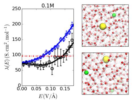
Figure 7: (left) High field behavior of the lower concentration, explicit solvent system in an ensemble with the field on both the water and the ions, $E_{\mathrm{i}}=E_{\mathrm{w}}=E$ (black) or just on the ions $E_{\mathrm{i}}=E$ and $E_{\mathrm{w}}=0$ (blue). Lines are computed from reweighting $p_{0}(J,Q)$, and symbols are computed from finite differences of $\left<J\right>_{E}$ versus $E$. Errorbars are one standard deviation of the mean. The red dashed line corresponds to the Nernst-Einstein molar ionic conductivity $\lambda_{\mathrm{id}}$. (right) Charactoristic snapshots from the molecular dynamics simulations at $E=0$ (top) and $E=0.15\mathrm{V/\AA}$ (bottom).

Appendix C High field behavior in the explicit model

While the ionic conductivity under the moderate field considered in Fig. 4 is weakly field-dependent, it does eventually grow quadratically under very high fields as shown in Fig. 7. The conductivity is found to exceed the Nernst-Einstein limit for free ions. However, this behavior is unphysical. Under fields higher than $E=0.1~{}\mathrm{V/\AA}$, in our molecular simulations, we find that the dipoles of the water molecule all align with the high field, restraining dipole fluctuations, and leading to dielectric breakdown. Further, water molecules will start to spontaneously dissociate at such high fields,Saitta, Saija, and Giaquinta (2012) which is not allowed due to the constraints on water molecules in our model.

References

References

- Harned and Owen (1959) H. S. Harned and B. B. Owen, Journal of The Electrochemical Society 106, 15C (1959).
- Zwanzig (1970) R. Zwanzig, The Journal of chemical physics 52, 3625 (1970).
- Onsager and Samaras (1934) L. Onsager and N. N. Samaras, The Journal of Chemical Physics 2, 528 (1934).
- Onsager and Fuoss (2002) L. Onsager and R. Fuoss, The Journal of Physical Chemistry 36, 2689 (2002).
- Kubo (1956) R. Kubo, Canadian Journal of Physics 34, 1274 (1956).
- Gao and Limmer (2019) C. Y. Gao and D. T. Limmer, Journal of Chemical Physics 151, 014101 (2019).
- Lesnicki et al. (2020) D. Lesnicki, C. Y. Gao, B. Rotenberg, and D. T. Limmer, Physical review letters 124, 206001 (2020).
- Bocquet and Charlaix (2010) L. Bocquet and E. Charlaix, Chemical Society Reviews 39, 1073 (2010).
- Bocquet (2020) L. Bocquet, Nature Materials 19, 254 (2020), number: 3 Publisher: Nature Publishing Group.
- Kavokine, Netz, and Bocquet (2021) N. Kavokine, R. R. Netz, and L. Bocquet, Annual Review of Fluid Mechanics 53, 377 (2021).
- Mouterde et al. (2019) T. Mouterde, A. Keerthi, A. Poggioli, S. Dar, A. Siria, A. Geim, L. Bocquet, and B. Radha, Nature 567, 87 (2019).
- Karnik et al. (2007) R. Karnik, C. Duan, K. Castelino, H. Daiguji, and A. Majumdar, Nano letters 7, 547 (2007).
- He et al. (2009) Y. He, D. Gillespie, D. Boda, I. Vlassiouk, R. S. Eisenberg, and Z. S. Siwy, Journal of the American Chemical Society 131, 5194 (2009).
- Picallo et al. (2013) C. B. Picallo, S. Gravelle, L. Joly, E. Charlaix, and L. Bocquet, Physical Review Letters 111, 244501 (2013).
- Cheng and Guo (2010) L.-J. Cheng and L. J. Guo, Chemical Society Reviews 39, 923 (2010), publisher: The Royal Society of Chemistry.
- Zwanzig (1965) R. Zwanzig, Annual Review of Physical Chemistry 16, 67 (1965).
- Seifert (2012) U. Seifert, Reports on progress in physics 75, 126001 (2012).
- Speck and Seifert (2006) T. Speck and U. Seifert, EPL (Europhysics Letters) 74, 391 (2006).
- Baiesi, Maes, and Wynants (2009) M. Baiesi, C. Maes, and B. Wynants, Physical review letters 103, 010602 (2009).
- Prost, Joanny, and Parrondo (2009) J. Prost, J.-F. Joanny, and J. Parrondo, Physical review letters 103, 090601 (2009).
- Dechant and Sasa (2020) A. Dechant and S.-i. Sasa, Proceedings of the National Academy of Sciences 117, 6430 (2020).
- Touchette (2018) H. Touchette, Physica A: Statistical Mechanics and its Applications 504, 5 (2018).
- Gao and Limmer (2017) C. Y. Gao and D. T. Limmer, Entropy 19, 571 (2017).
- Ray and Limmer (2019) U. Ray and D. T. Limmer, Physical Review B 100, 241409 (2019).
- Das and Limmer (2021) A. Das and D. T. Limmer, The Journal of Chemical Physics 154, 014107 (2021).
- GrandPre et al. (2021) T. GrandPre, K. Klymko, K. K. Mandadapu, and D. T. Limmer, Physical Review E 103, 012613 (2021).
- Wilson (1936) W. Wilson, The theory of the Wien effect for a binary electrolyte, Ph.D. thesis, PhD Thesis, Yale University (1936).
- Onsager and Kim (1957) L. Onsager and S. K. Kim, The Journal of Physical Chemistry 61, 198 (1957).
- Koneshan, Lynden-Bell, and Rasaiah (1998) S. Koneshan, R. M. Lynden-Bell, and J. C. Rasaiah, Journal of the American Chemical Society 120, 12041 (1998).
- Jardat et al. (1999) M. Jardat, O. Bernard, P. Turq, and G. R. Kneller, The Journal of chemical physics 110, 7993 (1999).
- Ladiges et al. (2021) D. R. Ladiges, A. Nonaka, K. Klymko, G. Moore, J. Bell, S. Carney, A. Garcia, S. Natesh, and A. Donev, Physical Review Fluids 6, 044309 (2021).
- Plimpton (1995) S. Plimpton, J. Comput. Phys. 117, 1 (1995).
- (33) “Large-scale Atomic/Molecular Massively Parallel Simulator,” https://lammps.sandia.gov, accessed: 2020-08-20.
- Kleinert (2009) H. Kleinert, Path integrals in quantum mechanics, statistics, polymer physics, and financial markets (World scientific, 2009).
- Girsanov (1960) I. V. Girsanov, Theory of Probability & Its Applications 5, 285 (1960).
- Basu and Maes (2015) U. Basu and C. Maes, in Journal of Physics: Conference Series, Vol. 638 (IOP Publishing, 2015) p. 012001.
- Earl and Deem (2005) D. J. Earl and M. W. Deem, Physical Chemistry Chemical Physics 7, 3910 (2005).
- Sugita, Kitao, and Okamoto (2000) Y. Sugita, A. Kitao, and Y. Okamoto, The Journal of Chemical Physics 113, 6042 (2000).
- Helfand (1960) E. Helfand, Physical Review 119, 1 (1960).
- Zwanzig (2001) R. Zwanzig, Nonequilibrium statistical mechanics (Oxford University Press, 2001).
- Frenkel and Smit (2001) D. Frenkel and B. Smit, Understanding molecular simulation: from algorithms to applications, Vol. 1 (Elsevier, 2001).
- Limmer et al. (2013) D. T. Limmer, C. Merlet, M. Salanne, D. Chandler, P. A. Madden, R. Van Roij, and B. Rotenberg, Physical review letters 111, 106102 (2013).
- Kumar et al. (1992) S. Kumar, J. M. Rosenberg, D. Bouzida, R. H. Swendsen, and P. A. Kollman, Journal of computational chemistry 13, 1011 (1992).
- Note (1) For historical context concerning the work of Wilson, reviewed extensively in Ref \rev@citealpnumharned1959physical but published only in his PhD thesis, see Ref \rev@citealpnumeu2010onsager.
- Hemmer, Holden, and Ratkje (1996) P. C. Hemmer, H. Holden, and S. K. Ratkje, The Collected Works of Lars Onsager (WORLD SCIENTIFIC, 1996).
- Eu (2010) B. C. Eu, arXiv:1005.5308 (2010).
- Yamada and Kawasaki (1967) T. Yamada and K. Kawasaki, Progress of Theoretical Physics 38, 1031 (1967).
- Morriss and Evans (1985) G. P. Morriss and D. J. Evans, Molecular Physics 54, 629 (1985).
- Crooks (2000) G. E. Crooks, Physical review E 61, 2361 (2000).
- Lesnicki and Vuilleumier (2017) D. Lesnicki and R. Vuilleumier, The Journal of chemical physics 147, 094502 (2017).
- Mangaud and Rotenberg (2020) E. Mangaud and B. Rotenberg, The Journal of Chemical Physics 153, 044125 (2020).
- Habershon, Markland, and Manolopoulos (2009) S. Habershon, T. E. Markland, and D. E. Manolopoulos, The Journal of Chemical Physics 131, 024501 (2009).
- Dufrêche et al. (2005) J.-F. Dufrêche, O. Bernard, S. Durand-Vidal, and P. Turq, The Journal of Physical Chemistry B 109, 9873 (2005).
- Chandler (1993) D. Chandler, Physical Review E 48, 2898 (1993).
- Speck (2013) T. Speck, Physical Review E 88, 014103 (2013).
- Pettitt and Rossky (1986) B. M. Pettitt and P. J. Rossky, The Journal of chemical physics 84, 5836 (1986).
- Sedlmeier et al. (2014) F. Sedlmeier, S. Shadkhoo, R. Bruinsma, and R. R. Netz, The Journal of Chemical Physics 140, 054512 (2014).
- Chandra and Bagchi (2000) A. Chandra and B. Bagchi, The Journal of Chemical Physics 112, 1876 (2000), publisher: American Institute of PhysicsAIP.
- Dufrêche et al. (2002) J.-F. Dufrêche, O. Bernard, P. Turq, A. Mukherjee, and B. Bagchi, Physical Review Letters 88, 095902 (2002).
- Balos et al. (2020) V. Balos, S. Imoto, R. R. Netz, M. Bonn, D. J. Bonthuis, Y. Nagata, and J. Hunger, Nature Communications 11, 1611 (2020).
- Eyink, Lebowitz, and Spohn (1996) G. L. Eyink, J. L. Lebowitz, and H. Spohn, Journal of Statistical physics 83, 385 (1996).
- Péraud et al. (2017) J.-P. Péraud, A. J. Nonaka, J. B. Bell, A. Donev, and A. L. Garcia, Proceedings of the National Academy of Sciences 114, 10829 (2017).
- Donev et al. (2019) A. Donev, A. L. Garcia, J.-P. Péraud, A. J. Nonaka, and J. B. Bell, Current Opinion in Electrochemistry 13, 1 (2019).
- Démery and Dean (2016) V. Démery and D. S. Dean, Journal of Statistical Mechanics: Theory and Experiment 2016, 023106 (2016).
- Pean et al. (2015) C. Pean, B. Daffos, B. Rotenberg, P. Levitz, M. Haefele, P.-L. Taberna, P. Simon, and M. Salanne, Journal of the American Chemical Society 137, 12627 (2015).
- Simonnin et al. (2018) P. Simonnin, V. Marry, B. Noetinger, C. Nieto-Draghi, and B. Rotenberg, The Journal of Physical Chemistry C 122, 18484 (2018).
- Palmer et al. (2020) B. J. Palmer, J. Chun, J. F. Morris, C. J. Mundy, and G. K. Schenter, Physical Review E 102, 022129 (2020).
- Jin et al. (2020) Y. Jin, T. Ng, R. Tao, S. Luo, Y. Su, and Z. Li, Physical Review E 102, 033112 (2020).
- Robin, Kavokine, and Bocquet (2021) P. Robin, N. Kavokine, and L. Bocquet, arXiv preprint arXiv:2105.07904 (2021).
- Esfandiar et al. (2017) A. Esfandiar, B. Radha, F. Wang, Q. Yang, S. Hu, S. Garaj, R. Nair, A. Geim, and K. Gopinadhan, Science 358, 511 (2017).
- Wettstein, Diddens, and Heuer (2021) A. Wettstein, D. Diddens, and A. Heuer, Macromolecules 54, 2256 (2021).
- (72) D. Lesnicki, C. Y. Gao, D. T. Limmer, and B. Rotenberg, Zendo, v1.0, Dataset https://doi.org/10.5281/zenodo.4660193 .
- Lebowitz and Percus (1966) J. Lebowitz and J. Percus, Physical Review 144, 251 (1966).
- Saitta, Saija, and Giaquinta (2012) A. M. Saitta, F. Saija, and P. V. Giaquinta, Physical review letters 108, 207801 (2012).