Boosting Binary Masks for Multi-Domain Learning through Affine Transformations

Abstract

In this work, we present a new, algorithm for multi-domain learning. Given a pretrained architecture and a set of visual domains received sequentially, the goal of multi-domain learning is to produce a single model performing a task in all the domains together. Recent works showed how we can address this problem by masking the internal weights of a given original conv-net through learned binary variables. In this work, we provide a general formulation of binary mask based models for multi-domain learning by affine transformations of the original network parameters. Our formulation obtains significantly higher levels of adaptation to new domains, achieving performances comparable to domain-specific models while requiring slightly more than 1 bit per network parameter per additional domain. Experiments on two popular benchmarks showcase the power of our approach, achieving performances close to state-of-the-art methods on the Visual Decathlon Challenge.

1 Introduction

A crucial requirement for visual systems is the ability to adapt an initial pretrained model to novel application domains. Achieving this goal requires facing multiple challenges. First, learning a new domain should not negatively affect the performance on old domains. Secondly, we should avoid adding many parameters to the model for each new domain that we want to learn, to ensure scalability. In this context, while deep learning algorithms have achieved impressive results on many computer vision benchmarks krizhevsky2012imagenet ; he2016deep ; girshick2014rich ; long2015fully , mainstream approaches for adapting deep models to novel domains tend to suffer from the problems mentioned above. In fact, fine-tuning a given architecture to new data does produce a powerful model on the novel domain, at the expense of degraded performance on the old ones, resulting in the well-known phenomenon of catastrophic forgetting french1999catastrophic ; goodfellow2013empirical . At the same time, replicating the network parameters and training a separate network for each domain is a powerful approach that preserves performances on old domains, but at the cost of an explosion of the network parameters rebuffi2017learning .

Different works addressed these problems by either considering losses encouraging the preservation of the current weights li2017learning ; kirkpatrick2017overcoming or by designing domain-specific network parameters rusu2016progressive ; rebuffi2017learning ; rosenfeld2017incremental ; mallya2017packnet ; mallya2018piggyback . Interestingly, in mallya2018piggyback ; mancini2018adding the authors showed that an effective strategy for achieving good multi-domain learning performances with a minimal increase in terms of network size is to create a binary mask for each domain. In mallya2018piggyback this mask is then multiplied by the main network weights, determining which of them are useful for addressing the new domain. Similarly, in mancini2018adding the masks are used as a scaled additive component to the network weights.

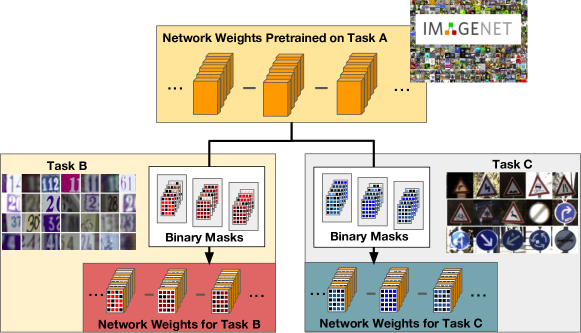
Figure 1: Idea behind our approach. A network pretrained on a given recognition domain A (i.e. ImageNet) can be extended to tackle other recognition domains B (e.g. digits) and C (e.g. traffic sign) by simply transforming the network weights (orange cubes) through domain-specific binary masks (colored grids).

In this work, we take inspiration from mallya2018piggyback ; mancini2018adding , formulating multi-domain learning as the problem of learning a transformation of a baseline, pretrained network, in a way to maximize the performance on a new domain. Importantly, the transformation should be compact in the sense of limiting the number of additional parameters required with respect to the baseline network. To this extent, we apply an affine transformation to each convolutional weight of the baseline network, which involves both a learned binary mask and a few additional parameters. The binary mask is used as a scaled and shifted additive component and as a multiplicative filter to the original weights. Figure 1 shows an example application of our algorithm. Given a network pretrained on a particular domain (i.e. ImageNet russakovsky2015imagenet , orange blocks) we can transform its original weights through binary masks (colored grids) and obtain a network which effectively addresses a novel domain (e.g. digit netzer2011reading or traffic sign stallkamp2012man recognition). Our solution allows to achieve two main goals: 1) boosting the performance of each domain-specific network that we train, by leveraging the higher degree of freedom in transforming the baseline network, while 2) keeping a low per-domain overhead in terms of additional parameters (slightly more than 1 bit per parameter per domain).

We assess the validity of our method, and some variants thereof, on standard benchmarks including the Visual Decathlon Challenge rebuffi2017learning . The experimental results show that our model achieves performances comparable with fine-tuning separate networks for each recognition domain on all benchmarks while retaining a very small overhead in terms of additional parameters per domain. Notably, we achieve results comparable to state-of-the-art models on the Visual Decathlon Challenge rebuffi2017learning but without requiring multiple training stages Li_2019_CVPR or a large number of domain-specific parameters Guo_2019_CVPR ; rebuffi2018efficient .

This paper extends our earlier work mancini2018adding in many aspects. In particular, we provide a general formulation of binary mask based methods for multi-domain learning, with mancini2018adding and mallya2018piggyback obtained as special cases. We show how this general formulation allows boosting the performances of binary mask based methods in multiple scenarios, achieving close to state-of-the-art results in the Visual Domain Decathlon Challenge. Finally, we significantly expand our experimental evaluation by 1) considering more recent multi-domain learning methods, 2) ablating the various components of our model as well as various design choices and 3) showing additional quantitative and qualitative results, employing multiple backbone architectures.

2 Related works

Multi-domain Learning. The need for visual models capable of addressing multiple domains received a lot of attention in recent years for what concerns both multi-task learning zamir2018taskonomy ; liu2019end ; cermelli2019rgb and multi-domain learning rebuffi2017learning ; rosenfeld2017incremental . Multi-task learning focuses on learning multiple visual tasks (e.g. semantic segmentation, depth estimation liu2019end ) with a single architecture. On the other hand, the goal of multi-domain learning is building a model able to address a task (e.g. classification) in multiple visual domains (e.g. real photos, digits) without forgetting previous domains and by using fewer parameters possible. An important work in this context is bilen2017universal , where the authors showed how multi-domain learning can be addressed by using a network sharing all parameters except for batch-normalization (BN) layers ioffe2015batch . In rebuffi2017learning , the authors introduced the Visual Domain Decathlon Challenge, a first multi-domain learning benchmark. The first attempts in addressing this challenge involved domain-specific residual components added in standard residual blocks, either in series rebuffi2017learning or in parallel rebuffi2018efficient , In rosenfeld2017incremental the authors propose to use controller modules where the parameters of the base architecture are recombined channel-wise, while in liu2019end exploits domain-specific attention modules. Other effective approaches include devising instance-specific fine-tuning strategies Guo_2019_CVPR , target-specific architectures Morgado_2019_CVPR and learning covariance normalization layers Li_2019_CVPR .

In mallya2017packnet only a reserved subset of network parameters is considered for each domain. The intersection of the parameters used by different domains is empty, thus the network can be trained end-to-end for each domain. Obviously, as the number of domain increases, fewer parameters are available for each domain, with a consequent limitation on the performances of the network. To overcome this issue, in mallya2018piggyback the authors proposed a more compact and effective solution based on directly learning domain-specific binary masks. The binary masks determine which of the network parameters are useful for the new domain and which are not, changing the actual composition of the features extracted by the network. This approach inspired subsequent works, improving both either the power of the binary masks mancini2018adding or their amount of bits required, masking directly an entire channel berriel2019budget . In this work, we take inspiration from these last research trends. In particular, we generalize the design of the binary masks employed in mallya2018piggyback and mancini2018adding . In particular, we consider neither simple multiplicative binary masks nor simple affine transformations of the original weights mancini2018adding but a general and flexible formulation capturing both cases. Experiments show how our approach leads to a boost in the performances while using a comparable number of parameters per domain. Moreover, our approach achieves performances comparable to more complex models rebuffi2018efficient ; Morgado_2019_CVPR ; Li_2019_CVPR ; Guo_2019_CVPR in the challenging Visual Domain Decathlon challenge, largely reducing the gap of binary-mask based methods with the current state of the art.

Incremental Learning. The keen interest in incremental and life-long learning methods dates back to the pre-convnet era, with shallow learning approaches ranging from large margin classifiers KuzborskijOC13 ; KuzborskijOC17 to non-parametric methods MensinkVPC13 ; RistinGGG16 . In recent years, various works have addressed the problem of incremental and life-long learning within the framework of deep architectures RebuffiKSL17 ; GuerrieroCM18 ; BendaleB16 ; cermelli2020modeling . A major risk when training a neural network on a novel task/domain is to deteriorate the performances of the network on old domains, discarding previous knowledge. This phenomenon is called catastrophic forgetting mccloskey1989catastrophic ; french1999catastrophic ; goodfellow2013empirical . To address this issue, various works designed constrained optimization procedures taking into account the initial network weights, trained on previous domains. In li2017learning , the authors exploit knowledge distillation hinton2015distilling to obtain target objectives for previous domains/tasks, while training for novel ones. The additional objective ensures the preservation of the activation for previous domains, making the model less prone to experience the catastrophic forgetting problem. In kirkpatrick2017overcoming the authors consider computing the update of the network parameters, based on their importance for previously seen domains. While these approaches are optimal in terms of the required parameters, i.e. they maintain the same number of parameters of the original network, they limit the catastrophic forgetting problem to the expenses of lower performance on both old and new domains. Recent methods overcome this issue by devising domain-specific parameters which are added as new domains are learned. If the initial network parameters remain untouched, the catastrophic forgetting problem is avoided but at the cost of the additional parameters required. The extreme case is the work of rusu2016progressive in the context of reinforcement learning, where a parallel network is added each time a new domain is presented with side domain connections, exploited to improve the performances on novel domains.

Our work addresses catastrophic forgetting by adding domain-specific parameters, as in rusu2016progressive and the mask-based approaches mallya2017packnet ; mallya2018piggyback . However, our domain-specific parameters require lower overhead with respect to rusu2016progressive while at the same time being more effective than the ones in mallya2017packnet ; mallya2018piggyback .

Network Binarization. Due to the low overhead required by the binary domain-specific parameters, our method is linked to recent works on binarization courbariaux2016binarized ; hubara2016binarized ; rastegari2016xnor and quantization hubara2016quantized ; lin2016fixed ; zhou2016dorefa of network parameters. Binarization methods courbariaux2016binarized ; hubara2016binarized binarize network parameters and activations in order to obtain a lower computational cost, making the architecture usable in devices with constrained computational capabilities. Binarization can be performed at multiple levels. In courbariaux2016binarized ; hubara2016binarized , network weights and activations are binarized between -1 and 1 at run time and used to compute the parameters gradients. In rastegari2016xnor , standard dot products are replaced by XNOR operations among binarized parameters and inputs. A closely related research thread is network quantization hubara2016quantized , where instead of binary, low bitwidth networks and activations are considered. In zhou2016dorefa ; lin2015neural , also the network gradients are quantized, reducing the memory and computation footprint in the backward pass.

Similarly to these works, here we are interested in obtaining a network representation with a low memory footprint. However, opposite to these works, we compress neither the whole architecture nor its activations but a subset of its parameters (i.e. the domain-specific ones) in order to make the sequential extension to multiple domains scalable. Despite these differences, the optimization techniques used in these works (e.g. hubara2016binarized ) are fundamental building blocks of our algorithm.

3 Method

We address the problem of multi-domain learning, where we want to extend an architecture pretrained on a given task (e.g. ResNet-50 pretrained on ImageNet) to perform the same task (e.g. classification) in different domains (e.g. traffic signal classification, digits recognition) with different output spaces. As in mallya2017packnet ; mallya2018piggyback , we consider the case where we receive the different domains one at the time, in a sequential fashion. We highlight that the term sequential refers to the nature of the problem but our current formulation of the model extends the pretrained model one domain at the time, without considering the order in which the domains are received.

In this context, our goal is to maximize the performance of the base model on the new set of domains, while limiting the memory occupied by the additional parameters needed. The solution we propose exploits the key idea from Piggyback mallya2018piggyback of learning domain-specific masks, but instead of pursuing the simple multiplicative transformation of the parameters of the baseline network, we define a parametrized, affine transformation mixing a binary mask and real parameters that significantly increases the expressiveness of the approach, leading to a rich and nuanced ability to adapt the old parameters to the needs of the new domains. This brings considerable improvements on the conducted experiments, as we will show in the experimental section, while retaining a reduced, per-domain overhead.

3.1 Overview

Let us assume to be given a pretrained, baseline network $f_{0}(\cdot;\Theta,\Omega_{0}):\mathcal{X}\to\mathcal{Y}_{0}$ assigning a class label in $\mathcal{Y}_{0}$ to elements of an input space $\mathcal{X}$ (e.g. images). The parameters of the baseline network are partitioned into two sets: $\Theta$ comprises parameters that will be shared for other domains, whereas $\Omega_{0}$ entails the rest of the parameters (e.g. the classifier). Our goal is to learn for each domain $i\in\{1,\ldots,\mathsf{m}\}$, with a possibly different output space $\mathcal{Y}_{i}$, a classifier $f_{i}(\cdot;\Theta,\Omega_{i}):\mathcal{X}\to\mathcal{Y}_{i}$. Here, $\Omega_{i}$ entails the parameters specific for the $i$th domain, while $\Theta$ holds the shareable parameters of the baseline network mentioned above.

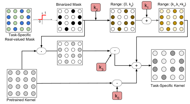
Figure 2: Overview of the proposed model (best viewed in color). Given a convolutional kernel, for each domain, we exploit a real-valued mask to generate a domain-specific binary mask. An affine transformation directly applied to the binary masks, which changes their range (through a scale parameter $k_{2}$) and their minimum value (through $k_{1}$). A multiplicative mask applied to the original kernels and the pretrained kernel themselves are scaled by the factors $k_{3}$ and $k_{0}$ respectively. All the different masks are summed to produce the final domain-specific kernel.

Each domain-specific network $f_{i}$ shares the same structure of the baseline network $f_{0}$, except for having a possibly differently sized classification layer. For each convolutional layer of $f_{0}$ with parameters $\mathtt{W}$, the domain-specific network $f_{i}$ holds a binary mask $\mathtt{M}$, with the same shape of $\mathtt{W}$, that is used to mask original filters. The way the mask is exploited to specialize the network filters produces different variants of our model, which we describe in the following.

3.2 Affine Weight Transformation through Binary Masks

Following previous works mallya2018piggyback ; mancini2018adding , we consider domain-specific networks $f_{i}$ that are shaped as the baseline network $f_{0}$ and we store in $\Omega_{i}$ a binary mask $\mathtt{M}$ for each convolutional kernel $\mathtt{W}$ in the shared set $\Theta$. However, differently from mallya2018piggyback ; mancini2018adding , we consider a more general affine transformation of the base convolutional kernel $\mathtt{W}$ that depends on a binary mask $\mathtt{M}$ as well as additional parameters. Specifically, we transform $\mathtt{W}$ into

$$\tilde{\mathtt{W}}=k_{0}\mathtt{W}+k_{1}\mathtt{1}+k_{2}\mathtt{M}+k_{3}\mathtt{W}\circ\mathtt{M}\,,$$ (1)

where $k_{j}\in\mathbb{R}$ are additional domain-specific parameters in $\Omega_{i}$ that we learn along with the binary mask $\mathtt{M}$, $\mathtt{1}$ is an opportunely sized tensor of $1$s, and $\circ$ is the Hadamard (or element-wise) product. The transformed parameters $\hat{\mathtt{W}}$ are then used in the convolutional layer of $f_{i}$. We highlight that the domain-specific parameters that are stored in $\Omega_{i}$ amount to just a single bit per parameter in each convolutional layer plus a few scalars per layer, yielding a low overhead per additional domain while retaining a sufficient degree of freedom to build new convolutional weights. Figure 2 provides an overview of the transformation in (1).

Our model, can be regarded as a parametrized generalization of mallya2018piggyback , since we can recover the formulation of mallya2018piggyback by setting $k_{0,1,2}=0$ and $k_{3}=1$. Similarly, if we get rid of the multiplicative component, i.e. we set $k_{3}=0$, we obtained the following simplified transformation

$$\check{\mathtt{W}}=k_{0}\mathtt{W}+k_{1}\mathtt{1}+k_{2}\mathtt{M}\,,$$ (2)

which corresponds to the method presented in our previous work mancini2018adding and will be taken into account in our analysis.

We want to highlight that each model (i.e. ours,mallya2018piggyback and mancini2018adding ) has different representation capabilities. In fact, in mallya2018piggyback , the domain-specific parameters can take only two possible values: either $0$ (i.e. if $m=0$) or the original pretrained weights (i.e. if $m=1$). On the other hand, the scalar components of our previous work mancini2018adding allow both scaling (i.e. with $k_{0}$) and shifting (i.e. with $k_{1}$) the original network weights, with the additive binary mask adding a bias term (i.e. $k_{2}$) selectively to a group of parameters (i.e. the one with $m=1$). Our work generalizes mallya2018piggyback and mancini2018adding by considering the multiplicative binary-mask term $\mathtt{W}\circ\mathtt{M}$ as an additional bias component scaled by the scalar $k_{3}$. In this way, our model has the possibility to obtain parameter-specific bias components, something that was not possible neither in mallya2018piggyback nor in mancini2018adding . The additional degrees of freedom makes the search space of our method larger with respect to mallya2018piggyback ; mancini2018adding , with the possibility to express more complex (and tailored) domain-specific transformations. Thus, as we show in the experimental section, the additional parameters that we introduce with our method bring a negligible per-domain overhead compared to mallya2018piggyback and mancini2018adding , which is nevertheless generously balanced out by a significant boost of the performance of the domain-specific classifiers.

Finally, following bilen2017universal ; mancini2018adding , we opt also for domain-specific batch-normalization parameters (i.e. mean, variance, scale and bias), unless otherwise stated. Those parameters will not be fixed (i.e. they do not belong to $\Theta$) but are part of $\Omega_{i}$, and thus optimized for each domain. As in mancini2018adding , in the cases where we have a convolutional layer followed by batch normalization, we keep the corresponding parameter $k_{0}$ fixed to $1$, because the output of batch normalization is invariant to the scale of the convolutional weights.

3.3 Learning Binary Masks

Given the training set of the $i_{th}$ domain, we learn the domain-specific parameters $\Omega_{i}$ by minimizing a standard supervised loss, i.e. the classification log-loss. However, while the domain-specific batch-normalization parameters can be learned by employing standard stochastic optimization methods, the same is not feasible for the binary masks. Indeed, optimizing the binary masks directly would turn the learning into a combinatorial problem. To address this issue, we follow the solution adopted in mallya2018piggyback ; mancini2018adding , i.e. we replace each binary mask $\mathtt{M}$ with a thresholded real matrix $\mathtt{R}$. By doing so, we shift from optimizing discrete variables in $\mathtt{M}$ to continuous ones in $\mathtt{R}$. However, the gradient of the hard threshold function $h(r)=1_{r\geq 0}$ is zero almost everywhere, making this solution apparently incompatible with gradient-based optimization approaches. To address this issue we consider a strictly increasing, surrogate function $\tilde{h}$ that will be used in place of $h$ only for the gradient computation, i.e.

$$h^{\prime}(r)\approx\tilde{h}^{\prime}(r)\,,$$

where $h^{\prime}$ denotes the derivative of $h$ with respect to its argument. The gradient that we obtain via the surrogate function has the property that it always points in the right down hill direction in the error surface. Let $r$ be a single entry of $\mathtt{R}$, with $m=h(r)$ and let $E(m)$ be the error function. Then

$$\operatorname{sgn}((E\circ h)^{\prime}(r))=\operatorname{sgn}(E^{\prime}(m)h^{\prime}(r))=\operatorname{sgn}\left(E^{\prime}(m)\tilde{h}^{\prime}(r)\right)$$

and, since $\tilde{h}^{\prime}(r)>0$ by construction of $\tilde{h}$, we obtain the sign agreement

$$\operatorname{sgn}\left((E\circ h)^{\prime}(r)\right)=\operatorname{sgn}\left(E^{\prime}(m)\right)\,.$$

Accordingly, when the gradient of $E(h(r))$ with respect to $r$ is positive (negative), this induces a decrease (increase) of $r$. By the monotonicity of $h$ this eventually induces a decrease (increase) of $m$, which is compatible with the direction pointed by the gradient of $E$ with respect to $m$.

In the experiments, we set $\tilde{h}(x)=x$, i.e. the identity function, recovering the workaround suggested in hin12 and employed also in mallya2018piggyback ; mancini2018adding . However, other choices are possible. For instance, by taking $\tilde{h}(x)=(1+e^{-x})^{-1}$, i.e. the sigmoid function, we obtain a better approximation that has been suggested in goodman1994learning ; bengio2013estimating . We test different choices for $\tilde{h}(x)$ in the experimental section.

4 Experiments

Datasets. In the following, we test our method on two different multi-domain benchmarks, where the multiple domains regard different classification tasks. For the first benchmark we follow mallya2018piggyback , and we use 6 datasets: ImageNet russakovsky2015imagenet , VGG-Flowers nilsback2008automated , Stanford Cars krause20133d , Caltech-UCSD Birds (CUBS) wah2011caltech , Sketches eitz2012humans and WikiArt saleh2015large . VGG-Flowers nilsback2008automated is a dataset of fine-grained recognition containing images of 102 categories, corresponding to different kind of flowers. There are 2’040 images for training and 6’149 for testing. Stanford Cars krause20133d contains images of 196 different types of cars with approximately 8 thousand images for training and 8 thousand for testing. Caltech-UCSD Birds wah2011caltech is another dataset of fine-grained recognition containing images of 200 different species of birds, with approximately 6 thousand images for training and 6 thousand for testing. Sketches eitz2012humans is a dataset composed of 20 thousand sketch drawings, 16 thousand for training and 4 thousand for testing. It contains images of 250 different objects in their sketched representations. WikiArt saleh2015large contains painting from 195 different artists. The dataset has 42’129 images for training and 10628 images for testing. These datasets contain a lot of variations both from the category addressed (i.e. cars krause20133d vs birds wah2011caltech ) and the appearance of their instances (from natural images russakovsky2015imagenet to paintings saleh2015large and sketches eitz2012humans ), thus representing a challenging benchmark for multi-domain learning techniques.

The second benchmark is the Visual Domain Decathlon Challenge rebuffi2017learning . This challenge has been introduced to check the capability of a single algorithm to tackle 10 different classification tasks. The tasks are taken from the following datasets: ImageNet russakovsky2015imagenet , CIFAR-100 krizhevsky2009learning , Aircraft maji2013fine , Daimler pedestrian classification (DPed) munder2006experimental , Describable textures (DTD) cimpoi2014describing , German traffic signs (GTSR) stallkamp2012man , Omniglot lake2015human , SVHN netzer2011reading , UCF101 Dynamic Images bilen2016dynamic ; soomro2012ucf101 and VGG-Flowers nilsback2008automated . A more detailed description of the challenge and the datasets can be found in rebuffi2017learning . For this challenge, an independent scoring function is defined rebuffi2017learning . This function $S$ is expressed as:

$$S=\sum^{10}_{d=1}\alpha_{d}\text{max}\{0,E_{d}^{\text{max}}-E_{d}\}^{2}$$ (3)

where $E_{d}^{\text{max}}$ is the test error of the baseline in the domain $d$, $E_{d}$ is the test error of the submitted model and $\alpha$ is a scaling parameter ensuring that the perfect score for each domain is 1000, thus with a maximum score of 10000 for the whole challenge. The baseline error is computed doubling the error of 10 independent models fine-tuned on the single domains. This score function takes into account the performances of a model on all 10 classes, preferring models with good performances on all of them compared to models outperforming by a large margin the baseline in just a few. Following berriel2019budget , we use this metric also for the first benchmark, keeping the same upper-bound of 1000 points for each domain. Moreover, as in berriel2019budget , we report the ratio among the score obtained and the parameters used, denoting it as ${S}_{p}$. This metric allows capturing the trade-off among the performances and model size.

Networks and training protocols. For the first benchmark, we use 3 networks: ResNet-50 he2016deep , DenseNet-121 huang2017densely and VGG-16 simonyan2014very , reporting the results of Piggyback mallya2018piggyback , PackNet mallya2017packnet and both the simple mancini2018adding and full version of our model described in Section 3.

Following the protocol of mallya2018piggyback , for all the models we start from the networks pretrained on ImageNet and train the domain-specific networks using Adam kingma2014adam as optimizer except for the classifiers where SGD bottou2010large with momentum is used. The networks are trained with a batch-size of 32 and an initial learning rate of 0.0001 for Adam and 0.001 for SGD with momentum 0.9. Both the learning rates are decayed by a factor of 10 after 15 epochs. In this scenario, we use input images of size $224\times 224$ pixels, with the same data augmentation (i.e. mirroring and random rescaling) of mallya2017packnet ; mallya2018piggyback . The real-valued masks are initialized with random values drawn from a uniform distribution with values between $0.0001$ and $0.0002$. Since our model is independent of the order of the domains, we do not take into account different possible orders, reporting the results as accuracy averaged across multiple runs. For simplicity, in the following, we will denote this scenario as ImageNet-to-Sketch.

For the Visual Domain Decathlon, we employ the Wide ResNet-28 zagoruyko2016wide adopted by previous methods rebuffi2017learning ; rosenfeld2017incremental ; mallya2018piggyback , with a widening factor of 4 (i.e. 64, 128 and 256 channels in each residual block). Following rebuffi2017learning we rescale the input images to $72\times 72$ pixels giving as input to the network images cropped to $64\times 64$. We follow the protocol in mallya2018piggyback , by training the simple and full versions of our model for 60 epochs for each domain, with a batch-size of 32, and using again Adam for the entire architecture but the classifier, where SGD with momentum is used. The same learning rates of the first benchmark are adopted and are decayed by a factor of 10 after 45 epochs. Similarly, the same initialization scheme is used for the real-valued masks. No hyperparameter tuning has been performed as we used a single training schedule for all the 10 domains, except for the ImageNet pretrained model, which was trained following the schedule of rebuffi2017learning . As for data augmentation, mirroring has been performed, except for the datasets with digits (i.e. SVHN), signs (Omniglot, GTSR) and textures (i.e. DTD) as it may be rather harmful (as in the first 2 cases) or unnecessary.

In both benchmarks, we train our network on one domain at the time, sequentially for all domains. For each domain, we introduce the domain-specific binary masks and additional scalar parameters, as described in section 3. Moreover, following previous approaches rebuffi2017learning ; rebuffi2018efficient ; mallya2018piggyback ; rosenfeld2017incremental , we consider a separate classification layer for each domain. This is reflected also in the computation of the parameters overhead required by our model, we do not consider the separate classification layers, following comparison systems rebuffi2017learning ; rebuffi2018efficient ; mallya2018piggyback ; rosenfeld2017incremental .

4.1 Results

ImageNet-to-Sketch. In the following, we discuss the results obtained by our model on the ImageNet-to-Sketch scenario. We compare our method with Piggyback mallya2018piggyback , PackNet mallya2017packnet and two baselines considering (i) the network only as feature extractor, training only the domain-specific classifier, and (ii) individual networks separately fine-tuned on each domain. PackNet mallya2017packnet adds a new domain to a pretrained architecture by identifying which weights are important for the domain, optimizing the architecture through alternated pruning and re-training steps. Since this algorithm is dependent on the order of the domains, we report the performances for two different orderings mallya2018piggyback : starting from the model pretrained on ImageNet, in the first setting ($\downarrow$) the order is CUBS-Cars-Flowers-WikiArt-Sketch while for the second ($\uparrow$) the order is reversed. For our model, we evaluate both the full and the simple version, including domain-specific batch-normalization layers. Since including batch-normalization layers affects the performances, for the sake of presenting a fair comparison, we report also the results of Piggyback mallya2018piggyback obtained as a special case of our model with separate BN parameters per domain for ResNet-50 and DenseNet-121. Moreover, we report the results of the Budget-Aware adapters ($\text{BA}^{2}$) method in berriel2019budget . This method relies on binary masks applied not per-parameter but per-channel, with a budget constraint allowing to further squeeze the network complexity. As in our method, also in berriel2019budget domain-specific BN layers are used.

Results are reported in Tables 1, 2 and 3. We see that both versions of our model are able to fill the gap between the classifier only baseline and the individual fine-tuned architectures almost entirely and in all settings. For larger and more diverse datasets such as Sketch and WikiArt, the gap is not completely covered, but the distance between our models and the individual architectures is always less than 1%. These results are remarkable given the simplicity of our method, not involving any assumption of the optimal weights per domain mallya2017packnet , and the small overhead in terms of parameters that we report in the row ”# Params” (i.e. $1.17$ for ResNet-50, $1.21$ for DenseNet-121 and $1.16$ for VGG-16), which represents the total number of parameters (counting all domains and excluding the classifiers) relative to the ones in the baseline network. For what concerns the comparison with the other algorithms, our model consistently outperforms both the basic version of Piggyback and PackNet in all the settings and architectures, except Sketch for the DenseNet and VGG-16 architectures and CUBS for VGG-16, in which the performances are comparable with those of Piggyback. When domain-specific BN parameters are introduced also for Piggyback (Tables 1 and 2), the gap in performances is reduced, with performances comparable to those of our model in some settings (i.e. CUBS) but with still large gaps in others (i.e. Flowers, Stanford Cars and WikiArt). These results show that the advantages of our model are not only due to the additional BN parameters, but also to the more flexible and powerful affine transformation introduced. This statement is further confirmed with the VGG-16 experiments in Table 3. For this network, when the standard Piggyback model is already able to fill the gap between the feature extractor baseline and the individual architectures, our model achieves either comparable or slightly superior performances (i.e. CUBS, WikiArt and Sketch). However, in the scenarios where Piggyback does not reach the performances of the independently fine-tuned models (i.e. Stanford Cars and Flowers), our model consistently outperforms the baseline, either halving (Flowers) or removing (Stanford Cars) the remained gap. Since this network does not contain batch-normalization layers, it confirms the generality of our model, showing the advantages of both our simple and full versions, even without domain-specific BN layers.

For what concerns the comparison with $\text{BA}^{2}$, the performances of our model are either comparable or superior in most of the settings. Remarkable are the gaps in the WikiArt dataset, with our full model surpassing $\text{BA}^{2}$ by 3% with ResNet-50 and 4% for DenseNet-121. Despite both Piggyback and $\text{BA}^{2}$ use fewer parameters than our approach, our full model outperforms both of them in terms of the final score (Score row) and the ratio among the score and the parameters used (Score/Params row). This shows that our model is the most powerful in making use of the binary masks, achieving not only higher performances but also a more favorable trade-off between performances and model size.

Finally, both Piggyback, $\text{BA}^{2}$ and our model outperform PackNet and, as opposed to the latter method, do not suffer from the heavy dependence on the ordering of the domains. This advantage stems from having a multi-domain learning strategy that is domain-independent, with the base network not affected by the new domains that are learned.

Table 1: Accuracy of ResNet-50 architectures in the ImageNet-to-Sketch scenario.

Dataset	Classifier	PackNetmallya2018piggyback		Piggyback		$\text{BA}^{2}$	Ours		Individual
	Only mallya2018piggyback	$\downarrow$	$\uparrow$	mallya2018piggyback	BN	berriel2019budget	Simple	Full	mallya2018piggyback
# Params	1	1.10		1.16	1.17	1.03	1.17	1.17	6
ImageNet	76.2	75.7	75.7	76.2	76.2	76.2	76.2	76.2	76.2
CUBS	70.7	80.4	71.4	80.4	82.1	81.2	82.6	82.4	82.8
Stanford Cars	52.8	86.1	80.0	88.1	90.6	92.1	91.5	91.4	91.8
Flowers	86.0	93.0	90.6	93.5	95.2	95.7	96.5	96.7	96.6
WikiArt	55.6	69.4	70.3	73.4	74.1	72.3	74.8	75.3	75.6
Sketch	50.9	76.2	78.7	79.4	79.4	79.3	80.2	80.2	80.8
Score	533	732	620	934	1184	1265	1430	1458	1500
Score/Params	533	665	534	805	1012	1228	1222	1246	250

Table 2: Accuracy of DenseNet-121 architectures in the ImageNet-to-Sketch scenario.

Dataset	Classifier	PackNetmallya2018piggyback		Piggyback		$\text{BA}^{2}$	Ours		Individual
	Only mallya2018piggyback	$\downarrow$	$\uparrow$	mallya2018piggyback	BN	berriel2019budget	Simple	Full	mallya2018piggyback
# Params	1	1.11		1.15	1.21	1.17	1.21	1.21	6
ImageNet	74.4	74.4	74.4	74.4	74.4	74.4	74.4	74.4	74.4
CUBS	73.5	80.7	69.6	79.7	81.4	82.4	81.5	81.7	81.9
Stanford Cars	56.8	84.7	77.9	87.2	90.1	92.9	91.7	91.6	91.4
Flowers	83.4	91.1	91.5	94.3	95.5	96.0	96.7	96.9	96.5
WikiArt	54.9	66.3	69.2	72.0	73.9	71.5	75.5	75.7	76.4
Sketch	53.1	74.7	78.9	80.0	79.1	79.9	79.9	79.8	80.5
Score	324	685	607	946	1209	1434	1506	1534	1500
Score/Params	324	617	547	822	999	1226	1245	1268	250

Table 3: Accuracy of VGG-16 architectures in the ImageNet-to-Sketch scenario.

Dataset	Classifier	PackNetmallya2018piggyback		Piggyback	Ours		Individual
	Only mallya2018piggyback	$\downarrow$	$\uparrow$	mallya2018piggyback	Simple	Full	mallya2018piggyback
# Params	1	1.09		1.16	1.16	1.16	6
ImageNet	71.6	70.7	70.7	71.6	71.6	71.6	71.6
CUBS	63.5	77.7	70.3	77.8	77.4	77.4	77.4
Stanford Cars	45.3	84.2	78.3	86.1	87.2	87.3	87.0
Flowers	80.6	89.7	89.8	90.7	91.6	91.5	92.3
WikiArt	50.5	67.2	68.5	71.2	71.6	71.9	67.7
Sketch	41.5	71.4	75.1	76.5	76.5	76.7	76.4
Score	342	1152	979	1441	1530	1538	1500
Score/Params	342	1057	898	1243	1319	1326	250

Visual Decathlon Challenge. In this section, we report the results obtained on the Visual Decathlon Challenge. We compare our model with the baseline method Piggyback mallya2018piggyback (PB), the budget-aware adapters of berriel2019budget ($\text{BA}^{2}$), the improved version of the winning entry of the 2017 edition of the challenge rosenfeld2017incremental (DAN), the network with domain-specific parallel adapters rebuffi2018efficient (PA), the domain-specific attention modules of liu2019end (MTAN), the covariance normalization approach Li_2019_CVPR (CovNorm) and SpotTune Guo_2019_CVPR . We additionally report the baselines proposed by the authors of the challenge rebuffi2017learning . For the latter, we report the results of 5 models: the network used as feature extractor (Feature), 10 different models fine-tuned on the single domains (Finetune), the network with domain-specific residual adapter modules rebuffi2017learning (RA), the same model with increased weight decay (RA-decay) and the same architecture jointly trained on all 10 domains, in a round-robin fashion (RA-joint). The first two models are considered as references. For the parallel adapters approach rebuffi2018efficient we report also the version with a post-training low-rank decomposition of the adapters (PA-SVD). This approach extracts a domain-specific and a domain agnostic component from the learned adapters with the domain-specific components which are further fine-tuned on each domain. Additionally, we report the novel results of the residual adapters rebuffi2017learning as reported in rebuffi2018efficient (RA-N).

Similarly to rosenfeld2017incremental we tune the training schedule, jointly for the 10 domains, using the validation set, and evaluate the results obtained on the test set (via the challenge evaluation server) by a model trained on the union of the training and validation sets, using the validated schedule. As opposed to methods like rebuffi2017learning we use the same schedule for the 9 domains (except for the baseline pretrained on ImageNet), without adopting domain-specific strategies for setting the hyper-parameters. Moreover, we do not employ our algorithm while pretraining the ImageNet architecture as in rebuffi2017learning . For fairness, we additionally report the results obtained by our implementation of mallya2018piggyback using the same pretrained model, training schedule and data augmentation adopted for our algorithm (PB ours).

The results are reported in Table 4 in terms of the $S$-score (see, Eq. (3)) and $S_{p}$. In the first part of the table are shown the baselines (i.e. finetuned architectures and using the base network as feature extractor) while in the middle the models considering a sequential formulation of the problem, against which we compare. In the last part of the table we report, for fairness, the methods that do not consider a sequential multi-domain learning scenario since they either train on all the datasets jointly (RA-joint) or have a multi-process step considering all domains (PA-SVD).

From the table we can see that the full form of our model (F) achieves very high results, being the third best performing method in terms of $S$-score, behind only CovNorm and SpotTune and being comparable to PA. However, SpotTune uses a large amount of parameters (11x) and PA doubles the parameters of the original model. CovNorm uses a very low number of parameters but requires a two-stage pipeline. On the other hand, our model requires neither a large number of parameters (such as SpotTune and PA) nor a two-stage pipeline (as CovNorm) while achieving results close to the state of the art (215 points below CovNorm in terms of $S$-score). Compared to binary mask based approaches, our model surpasses PiggyBack of more than 600 points, $\text{BA}^{2}$ of 300 and the simple affine transformation presented in mancini2018adding of more than 200. It is worth highlighting that these results have been achieved without domain-specific hyperparameter tuning, differently from previous works e.g. rebuffi2017learning ; rebuffi2018efficient ; Li_2019_CVPR .

For what concerns the $S_{p}$ score, our model is the third-best performing model, behind $\text{BA}^{2}$ and CovNorm. We highlight however that CovNorm requires a two-stage pipeline to reduce the amount of parameters needed, while $\text{BA}^{2}$ is explicitly designed with the purpose of limiting the budget (i.e. parameters, flops) required by the model.

Table 4: Results in terms of $S$ and $S_{p}$ scores for the Visual Decathlon Challenge.

Method	#Params	ImNet	Airc.	C100	DPed	DTD	GTSR	Flwr.	Oglt.	SVHN	UCF	Score	${S}_{p}$
Feature rebuffi2017learning	1	59.7	23.3	63.1	80.3	45.4	68.2	73.7	58.8	43.5	26.8	544	544
Finetune rebuffi2017learning	10	59.9	60.3	82.1	92.8	55.5	97.5	81.4	87.7	96.6	51.2	2500	250
RArebuffi2017learning	2	59.7	56.7	81.2	93.9	50.9	97.1	66.2	89.6	96.1	47.5	2118	1059
RA-decayrebuffi2017learning	2	59.7	61.9	81.2	93.9	57.1	97.6	81.7	89.6	96.1	50.1	2621	1311
RA-Nrebuffi2018efficient	2	60.3	61.9	81.2	93.9	57.1	99.3	81.7	89.6	96.6	50.1	3159	1580
DAN rosenfeld2017incremental	2.17	57.7	64.1	80.1	91.3	56.5	98.5	86.1	89.7	96.8	49.4	2852	1314
PA rebuffi2018efficient	2	60.3	64.2	81.9	94.7	58.8	99.4	84.7	89.2	96.5	50.9	3412	1706
MTAN liu2019end	1.74	63.9	61.8	81.6	91.6	56.4	98.8	81.0	89.8	96.9	50.6	2941	1690
SpotTune Guo_2019_CVPR	11	60.3	63.9	80.5	96.5	57.1	99.5	85.2	88.8	96.7	52.3	3612	328
CovNorm Li_2019_CVPR	1.25	60.4	69.4	81.3	98.8	60.0	99.1	83.4	87.7	96.6	48.9	3713	2970
PB mallya2018piggyback	1.28	57.7	65.3	79.9	97.0	57.5	97.3	79.1	87.6	97.2	47.5	2838	2217
PB ours	1.28	60.8	52.3	80.0	95.1	59.6	98.7	82.9	85.1	96.7	46.9	2805	2191
$\text{BA}^{2}$ berriel2019budget	1.03	56.9	49.4	78.1	95.5	55.1	99.4	86.1	88.7	96.9	50.2	3199	3106
Ours (S) mancini2018adding	1.29	60.8	51.3	81.9	94.7	59.0	99.1	88.0	89.3	96.5	48.7	3263	2529
Ours (F)	1.29	60.8	52.8	82.0	96.2	58.7	99.2	88.2	89.2	96.8	48.6	3497	2711
PA-SVDrebuffi2018efficient	1.5	60.3	66.0	81.9	94.2	57.8	99.2	85.7	89.3	96.6	52.5	3398	2265
RA-jointrebuffi2017learning	2	59.2	63.7	81.3	93.3	57.0	97.5	83.4	89.8	96.2	50.3	2643	1322

4.2 Ablation Study

In the following, we analyze the impact of the various components of our model. In particular, we consider the impact of the parameters $k_{0}$, $k_{1}$, $k_{2}$, $k_{3}$ and the surrogate function $\tilde{h}$ on the final results of our model for the ResNet-50 and DenseNet-121 architectures in the ImageNet-to-Sketch scenario. Since the architectures contain batch-normalization layers, we set $k_{0}=1$ for our simplemancini2018adding and full versions and $k_{0}=0$ when we analyze the special case mallya2018piggyback . For the other parameters we adopt various choices: either we fix them to a constant to not take into account their impact, or we train them, to assess their particular contribution to the model. The surrogate function we use is the identity function $\tilde{h}(x)=x$ unless otherwise stated (i.e. with Sigmoid). The results of our analysis are shown in Tables 5 and 6.

As the Tables show, while the BN parameters allow a boost in the performances of Piggyback, adding $k_{1}$ to the model does not provide a further gain in performances. This does not happen for the simple version of our model: without $k_{1}$ our model is not able to fully exploit the presence of the binary masks, achieving comparable or even lower performances with respect to the Piggyback model. We also note that a similar drop affecting our Simple version mancini2018adding when bias was omitted.

Noticeable, the full versions with $k_{2}=0$ suffer a large decrease in performances in almost all settings (e.g. ResNet-50 Flowers from 96.7% to 91.0%), showing that the component that brings the largest benefits to our algorithm is the addition of the binary mask itself scaled by $k_{2}$ (i.e. $k_{2}\cdot\mathtt{M}$). This explains also the reason why the simple version achieves performance similar to the full version of our model. We finally note that there is a limited contribution brought by the standard Piggyback component (i.e. $k_{1}\cdot\mathtt{W}\circ\mathtt{M}$), compared to the new components that we have introduced in the transformation: in fact, there is a clear drop in performance in various scenarios (e.g. CUBS, Cars) when we set either $k_{1}=0$ or $k_{2}=0$. Consequently, as $k_{1}$ is introduced in our Simple model, the boost of performances is significant such that neither the inclusion of $k_{3}$, nor considering channel-wise parameters $k_{1}$ provides further gains. Slightly better results are achieved in larger datasets, such as WikiArt, with the additional parameters giving more capacity to the model, thus better handling the larger amount of information available in the dataset.

As to what concerns the choice of the surrogate $\tilde{h}$, no particular advantage has been noted when $\tilde{h}(x)=\sigma(x)$ with respect to the standard straight-through estimator ($\tilde{h}(x)=x$). This may be caused by the noisy nature of the straight-through estimator, which has the positive effect of regularizing the parameters, as shown in previous works bengio2013estimating ; neelakantan2015adding .

We also note that for DenseNet-121, as opposed to ResNet-50, setting $k_{1}$ to zero degrades the performance only in 1 out of 5 datasets (i.e. CUBS) while the other 4 are not affected, showing that the effectiveness of different components of the model is also dependent on the architecture used.

Table 5: Impact of the parameters $k_{0}$, $k_{1}$, $k_{2}$ and $k_{3}$ of our model using the ResNet-50 architectures in the ImageNet-to-Sketch scenario. ✓ denotes a learned parameter, while ^∗ denotes mallya2018piggyback obtained as a special case of our model.

Method	$k_{0}$	$k_{1}$	$k_{2}$	$k_{3}$	CUBS	CARS	Flowers	WikiArt	Sketch
Piggyback mallya2018piggyback	0	0	0	1	80.4	88.1	93.6	73.4	79.4
Piggyback∗	0	0	0	1	80.4	87.8	93.1	72.5	78.6
Piggyback∗ with BN	0	0	0	1	82.1	90.6	95.2	74.1	79.4
Piggyback∗ with BN	0	✓	0	1	81.9	89.9	94.8	73.7	79.9
Ours (Simple, no bias)	1	0	✓	0	80.8	90.3	96.1	73.5	80.0
Ours (Simple) mancini2018adding	1	✓	✓	0	82.6	91.5	96.5	74.8	80.2
Ours (Simple with Sigmoid)	1	✓	✓	0	82.6	91.4	96.4	75.2	80.2
Ours (Full, no bias)	1	0	✓	✓	80.7	90.2	96.0	72.0	78.8
Ours (Full, no $k_{2}$)	1	✓	0	✓	80.6	87.5	91.0	73.0	78.4
Ours (Full)	1	✓	✓	✓	82.4	91.4	96.7	75.3	80.2
Ours (Full with Sigmoid)	1	✓	✓	✓	82.7	91.4	96.6	75.2	80.2
Ours (Full, channel-wise)	1	✓	✓	✓	82.0	91.0	96.3	74.8	80.0

Table 6: Impact of the parameters $k_{0}$, $k_{1}$, $k_{2}$ and $k_{3}$ of our model using the DenseNet-121 architectures in the ImageNet-to-Sketch scenario. ✓ denotes a learned parameter, while ^∗ denotes mallya2018piggyback obtained as a special case of our model.

Method	$k_{0}$	$k_{1}$	$k_{2}$	$k_{3}$	CUBS	CARS	Flowers	WikiArt	Sketch
Piggyback mallya2018piggyback	0	0	0	1	79.7	87.2	94.3	72.0	80.0
Piggyback∗	0	0	0	1	80.0	86.6	94.4	71.9	78.7
Piggyback∗ with BN	0	0	0	1	81.4	90.1	95.5	73.9	79.1
Piggyback∗ with BN	0	✓	0	1	81.9	90.1	95.4	72.6	79.9
Ours (Simple, no bias)	1	0	✓	0	80.4	91.4	96.7	75.0	79.7
Ours (Simple) mancini2018adding	1	✓	✓	0	81.5	91.7	96.7	75.5	79.9
Ours (Simple with Sigmoid)	1	✓	✓	0	81.5	91.7	97.0	76.0	79.8
Ours (Full, no bias)	1	0	✓	✓	80.2	91.1	96.5	75.1	79.2
Ours (Full, no $k_{2}$)	1	✓	0	✓	79.8	87.2	91.8	73.2	78.1
Ours (Full)	1	✓	✓	✓	81.7	91.6	96.9	75.7	79.9
Ours (Full with Sigmoid)	1	✓	✓	✓	82.0	91.7	97.0	76.0	79.9
Ours (Full, channel-wise)	1	✓	✓	✓	81.4	91.6	96.5	75.5	79.9

4.3 Parameter Analysis

We analyze the values of the parameters $k_{1}$, $k_{2}$ and $k_{3}$ of one instance of our full model in the ImageNet-to-Sketch benchmark. We use two of the architectures employed in that scenario, i.e. ResNet-50 and DenseNet-121, and we plot the values of $k_{1}$, $k_{2}$ and $k_{3}$ as well as the percentage of 1s present inside the binary masks for different layers of the architectures. Together with those values, we report the percentage of 1s for the masks obtained through our implementation of Piggyback. Both models have been trained considering domain-specific batch-normalization parameters. The results are shown in Figures 3 and 4. In all scenarios, our model keeps almost half of the masks active across the whole architecture. Compared to the masks obtained by Piggyback, there are 2 differences: 1) Piggyback exhibits denser masks (i.e. with a larger portion of 1s), 2) the density of the masks in Piggyback tends to decrease as the depth of the layer increases. Both these aspects may be linked to the nature of our model: by having more flexibility through the affine transformation adopted, there is less need to keep active large part of the network, since a loss of information can be recovered through the other components of the model, as well as constraining a particular part of the architecture. For what concerns the value of the parameters $k_{1}$, $k_{2}$ and $k_{3}$ for both architectures $k_{2}$ and $k_{3}$ tend to have larger magnitudes with respect to $k_{1}$. Also, the values of $k_{2}$ and $k_{1}$ tend to have a different sign, which allows the term $k_{1}\mathtt{1}+k_{2}\mathtt{M}$ to span over positive and negative values. We also note that the transformation of the weights is more prominent as the depth increases, which is intuitively explained by the fact that the baseline network requires stronger adaptation to represent the higher-level concepts of different domains. This is even more evident for WikiArt and Sketch due to the variability that these datasets contain with respect to standard natural images.

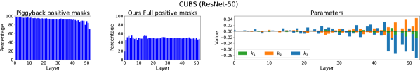
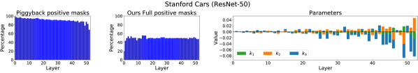
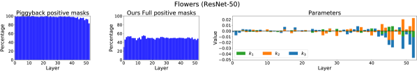
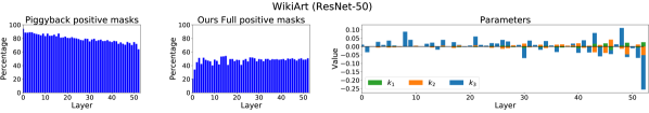
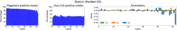
Figure 3: Percentage of 1s in the binary masks at different layers depth for Piggyback (left) and our full model (center) and values of the parameters $k_{1}$, $k_{2}$, $k_{3}$ computed by our full model (right) for all datasets of the Imagenet-to-Sketch benchmark and the ResNet-50 architecture.

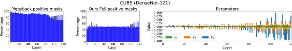
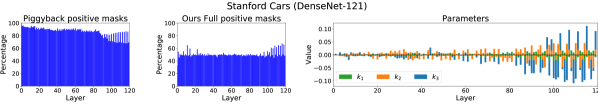
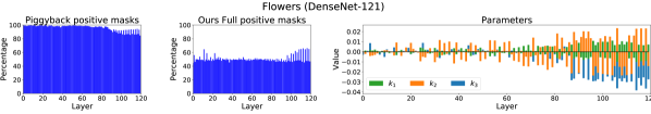
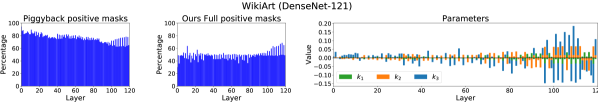
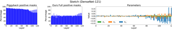
Figure 4: Percentage of 1s in the binary masks at different layers depth for Piggyback (left) and our full model (center) and values of the parameters $k_{1}$, $k_{2}$, $k_{3}$ computed by our full model (right) for all datasets of the Imagenet-to-Sketch benchmark with the DenseNet-121 architecture.

5 Conclusions

This work presents a simple yet powerful method for extending a pretrained deep architecture to novel visual domains. In particular, we generalize previous works on multi-domain learning applying binary masks to the original weights of the network mallya2018piggyback ; mancini2018adding by introducing an affine transformation that acts upon such weights and the masks themselves. Our generalization allows implementing a large variety of possible transformations, better adapting to the specific characteristic of each domain. These advantages are shown experimentally on two public benchmarks, fully confirming the power of our approach which fills the gap between the binary mask based and state-of-the-art methods on the Visual Decathlon Challenge.

Future work will explore the possibility to exploit this approach on several life-long learning scenarios, from incremental class learning RebuffiKSL17 ; li2017learning to open-world recognition bendale2015towardsowr ; mancini2019knowledge ; fontanel2020boosting . Moreover, while we assume to receive the new domains one by one in a sequential fashion, our current model tackles each visual domain independently. To this extent, an interesting research direction would be exploiting the relationship between different domains through cross-domain affine transformations, to force the model to reuse previous knowledge collected from different domains.

- (1) Bendale, A., Boult, T.: Towards open world recognition. In: CVPR (2015)
- (2) Bendale, A., Boult, T.E.: Towards open set deep networks. In: CVPR (2016)
- (3) Bengio, Y., Léonard, N., Courville, A.: Estimating or propagating gradients through stochastic neurons for conditional computation. arXiv preprint arXiv:1308.3432 (2013)
- (4) Berriel, R., Lathuilière, S., Nabi, M., Klein, T., Oliveira-Santos, T., Sebe, N., Ricci, E.: Budget-aware adapters for multi-domain learning. ICCV (2019)
- (5) Bilen, H., Fernando, B., Gavves, E., Vedaldi, A., Gould, S.: Dynamic image networks for action recognition. In: CVPR (2016)
- (6) Bilen, H., Vedaldi, A.: Universal representations: The missing link between faces, text, planktons, and cat breeds. arXiv preprint arXiv:1701.07275 (2017)
- (7) Bottou, L.: Large-scale machine learning with stochastic gradient descent. In: Proceedings of COMPSTAT’2010. Springer (2010)
- (8) Cermelli, F., Mancini, M., Bulò, S.R., Ricci, E., Caputo, B.: Modeling the background for incremental learning in semantic segmentation. In: CVPR (2020)
- (9) Cermelli, F., Mancini, M., Ricci, E., Caputo, B.: The rgb-d triathlon: Towards agile visual toolboxes for robots. In: IROS (2019)
- (10) Cimpoi, M., Maji, S., Kokkinos, I., Mohamed, S., Vedaldi, A.: Describing textures in the wild. In: CVPR (2014)
- (11) Courbariaux, M., Hubara, I., Soudry, D., El-Yaniv, R., Bengio, Y.: Binarized neural networks: Training deep neural networks with weights and activations constrained to+ 1 or-1. arXiv preprint arXiv:1602.02830 (2016)
- (12) Eitz, M., Hays, J., Alexa, M.: How do humans sketch objects? ACM Transactions on Graphics 31(4), 44–1 (2012)
- (13) Fontanel, D., Cermelli, F., Mancini, M., Bulò, S.R., Ricci, E., Caputo, B.: Boosting deep open world recognition by clustering. arXiv preprint arXiv:2004.13849 (2020)
- (14) French, R.M.: Catastrophic forgetting in connectionist networks. Trends in cognitive sciences 3(4), 128–135 (1999)
- (15) Girshick, R., Donahue, J., Darrell, T., Malik, J.: Rich feature hierarchies for accurate object detection and semantic segmentation. In: CVPR (2014)
- (16) Goodfellow, I.J., Mirza, M., Xiao, D., Courville, A., Bengio, Y.: An empirical investigation of catastrophic forgetting in gradient-based neural networks. arXiv preprint arXiv:1312.6211 (2013)
- (17) Goodman, R.M., Zeng, Z.: A learning algorithm for multi-layer perceptrons with hard-limiting threshold units. In: NIPS Workshops (1994)
- (18) Guerriero, S., Caputo, B., Mensink, T.: Deep nearest class mean classifiers. In: ICLR Worskhops (2018)
- (19) Guo, Y., Shi, H., Kumar, A., Grauman, K., Rosing, T., Feris, R.: Spottune: Transfer learning through adaptive fine-tuning. In: CVPR (2019)
- (20) He, K., Zhang, X., Ren, S., Sun, J.: Deep residual learning for image recognition. In: CVPR (2016)
- (21) Hinton, G.: Neural networks for machine learning (2012). Coursera, video lectures.
- (22) Hinton, G., Vinyals, O., Dean, J.: Distilling the knowledge in a neural network. arXiv preprint arXiv:1503.02531 (2015)
- (23) Huang, G., Liu, Z., Weinberger, K.Q., van der Maaten, L.: Densely connected convolutional networks. In: CVPR (2017)
- (24) Hubara, I., Courbariaux, M., Soudry, D., El-Yaniv, R., Bengio, Y.: Binarized neural networks. In: NIPS (2016)
- (25) Hubara, I., Courbariaux, M., Soudry, D., El-Yaniv, R., Bengio, Y.: Quantized neural networks: Training neural networks with low precision weights and activations. JMLR 18(187), 1–30 (2018)
- (26) Ioffe, S., Szegedy, C.: Batch normalization: Accelerating deep network training by reducing internal covariate shift. In: ICML (2015)
- (27) Kingma, D.P., Ba, J.: Adam: A method for stochastic optimization. arXiv preprint arXiv:1412.6980 (2014)
- (28) Kirkpatrick, J., Pascanu, R., Rabinowitz, N., Veness, J., Desjardins, G., Rusu, A.A., Milan, K., Quan, J., Ramalho, T., Grabska-Barwinska, A., et al.: Overcoming catastrophic forgetting in neural networks. Proceedings of the National Academy of Sciences 114(13), 3521–3526 (2017)
- (29) Krause, J., Stark, M., Deng, J., Fei-Fei, L.: 3d object representations for fine-grained categorization. In: ICCV Workshops (2013)
- (30) Krizhevsky, A., Hinton, G.: Learning multiple layers of features from tiny images (2009)
- (31) Krizhevsky, A., Sutskever, I., Hinton, G.E.: Imagenet classification with deep convolutional neural networks. In: NIPS (2012)
- (32) Kuzborskij, I., Orabona, F., Caputo, B.: From N to N+1: multiclass transfer incremental learning. In: CVPR (2013)
- (33) Kuzborskij, I., Orabona, F., Caputo, B.: Scalable greedy algorithms for transfer learning. CVIU 156, 174–185 (2017)
- (34) Lake, B.M., Salakhutdinov, R., Tenenbaum, J.B.: Human-level concept learning through probabilistic program induction. Science 350(6266), 1332–1338 (2015)
- (35) Li, Y., Vasconcelos, N.: Efficient multi-domain learning by covariance normalization. In: CVPR (2019)
- (36) Li, Z., Hoiem, D.: Learning without forgetting. IEEE T-PAMI (2017)
- (37) Lin, D., Talathi, S., Annapureddy, S.: Fixed point quantization of deep convolutional networks. In: ICML (2016)
- (38) Lin, Z., Courbariaux, M., Memisevic, R., Bengio, Y.: Neural networks with few multiplications. arXiv preprint arXiv:1510.03009 (2015)
- (39) Liu, S., Johns, E., Davison, A.J.: End-to-end multi-task learning with attention. In: CVPR (2019)
- (40) Long, J., Shelhamer, E., Darrell, T.: Fully convolutional networks for semantic segmentation. In: CVPR (2015)
- (41) Maji, S., Rahtu, E., Kannala, J., Blaschko, M., Vedaldi, A.: Fine-grained visual classification of aircraft. arXiv preprint arXiv:1306.5151 (2013)
- (42) Mallya, A., Lazebnik, S.: Packnet: Adding multiple tasks to a single network by iterative pruning. In: CVPR (2018)
- (43) Mallya, A., Lazebnik, S.: Piggyback: Adding multiple tasks to a single, fixed network by learning to mask. arXiv preprint arXiv:1801.06519 (2018)
- (44) Mancini, M., Karaoguz, H., Ricci, E., Jensfelt, P., Caputo, B.: Knowledge is never enough: Towards web aided deep open world recognition. In: ICRA (2019)
- (45) Mancini, M., Ricci, E., Caputo, B., Rota Bulò, S.: Adding new tasks to a single network with weight transformations using binary masks. In: ECCV-WS (2018)
- (46) McCloskey, M., Cohen, N.J.: Catastrophic interference in connectionist networks: The sequential learning problem. In: Psychology of learning and motivation, vol. 24, pp. 109–165. Elsevier (1989)
- (47) Mensink, T., Verbeek, J.J., Perronnin, F., Csurka, G.: Distance-based image classification: Generalizing to new classes at near-zero cost. IEEE T-PAMI 35(11), 2624–2637 (2013)
- (48) Morgado, P., Vasconcelos, N.: Nettailor: Tuning the architecture, not just the weights. In: CVPR (2019)
- (49) Munder, S., Gavrila, D.M.: An experimental study on pedestrian classification. IEEE T-PAMI 28(11), 1863–1868 (2006)
- (50) Neelakantan, A., Vilnis, L., Le, Q.V., Sutskever, I., Kaiser, L., Kurach, K., Martens, J.: Adding gradient noise improves learning for very deep networks. arXiv preprint arXiv:1511.06807 (2015)
- (51) Netzer, Y., Wang, T., Coates, A., Bissacco, A., Wu, B., Ng, A.Y.: Reading digits in natural images with unsupervised feature learning. In: NIPS Workshops (2011)
- (52) Nilsback, M.E., Zisserman, A.: Automated flower classification over a large number of classes. In: Computer Vision, Graphics & Image Processing, 2008. ICVGIP’08. Sixth Indian Conference on. IEEE (2008)
- (53) Rastegari, M., Ordonez, V., Redmon, J., Farhadi, A.: Xnor-net: Imagenet classification using binary convolutional neural networks. In: ECCV (2016)
- (54) Rebuffi, S., Kolesnikov, A., Sperl, G., Lampert, C.H.: icarl: Incremental classifier and representation learning. In: CVPR (2017)
- (55) Rebuffi, S.A., Bilen, H., Vedaldi, A.: Learning multiple visual domains with residual adapters. In: NIPS (2017)
- (56) Rebuffi, S.A., Bilen, H., Vedaldi, A.: Efficient parametrization of multi-domain deep neural networks. In: CVPR (2018)
- (57) Ristin, M., Guillaumin, M., Gall, J., Gool, L.J.V.: Incremental learning of random forests for large-scale image classification. IEEE T-PAMI 38(3), 490–503 (2016)
- (58) Rosenfeld, A., Tsotsos, J.K.: Incremental learning through deep adaptation. arXiv preprint arXiv:1705.04228 (2017)
- (59) Russakovsky, O., Deng, J., Su, H., Krause, J., Satheesh, S., Ma, S., Huang, Z., Karpathy, A., Khosla, A., Bernstein, M., et al.: Imagenet large scale visual recognition challenge. IJCV 115(3), 211–252 (2015)
- (60) Rusu, A.A., Rabinowitz, N.C., Desjardins, G., Soyer, H., Kirkpatrick, J., Kavukcuoglu, K., Pascanu, R., Hadsell, R.: Progressive neural networks. arXiv preprint arXiv:1606.04671 (2016)
- (61) Saleh, B., Elgammal, A.: Large-scale classification of fine-art paintings: Learning the right metric on the right feature. In: International Conference on Data Mining Workshops (2015)
- (62) Simonyan, K., Zisserman, A.: Very deep convolutional networks for large-scale image recognition. In: ICLR (2015)
- (63) Soomro, K., Zamir, A.R., Shah, M.: Ucf101: A dataset of 101 human actions classes from videos in the wild. arXiv preprint arXiv:1212.0402 (2012)
- (64) Stallkamp, J., Schlipsing, M., Salmen, J., Igel, C.: Man vs. computer: Benchmarking machine learning algorithms for traffic sign recognition. Neural networks 32, 323–332 (2012)
- (65) Wah, C., Branson, S., Welinder, P., Perona, P., Belongie, S.: The caltech-ucsd birds-200-2011 dataset (2011)
- (66) Zagoruyko, S., Komodakis, N.: Wide residual networks. In: BMVC (2016)
- (67) Zamir, A.R., Sax, A., Shen, W., Guibas, L.J., Malik, J., Savarese, S.: Taskonomy: Disentangling task transfer learning. In: CVPR (2018)
- (68) Zhou, S., Wu, Y., Ni, Z., Zhou, X., Wen, H., Zou, Y.: Dorefa-net: Training low bitwidth convolutional neural networks with low bitwidth gradients. arXiv preprint arXiv:1606.06160 (2016)