Abstract

This paper considers batch Reinforcement Learning (RL) with general value function approximation. Our study investigates the minimal assumptions to reliably estimate/minimize Bellman error, and characterizes the generalization performance by (local) Rademacher complexities of general function classes, which makes initial steps in bridging the gap between statistical learning theory and batch RL. Concretely, we view the Bellman error as a surrogate loss for the optimality gap, and prove the followings: (1) In double sampling regime, the excess risk of Empirical Risk Minimizer (ERM) is bounded by the Rademacher complexity of the function class. (2) In the single sampling regime, sample-efficient risk minimization is not possible without further assumptions, regardless of algorithms. However, with completeness assumptions, the excess risk of FQI and a minimax style algorithm can be again bounded by the Rademacher complexity of the corresponding function classes. (3) Fast statistical rates can be achieved by using tools of local Rademacher complexity. Our analysis covers a wide range of function classes, including finite classes, linear spaces, kernel spaces, sparse linear features, etc.

1 Introduction

Statistical learning theory, since its introduction in the late 1960’s, has become one of the most important frameworks in machine learning, to study problems of inference or function estimation from a given collection of data (Hastie et al., 2009; Vapnik, 2013; James et al., 2013). The development of statistical learning has led to a series of new popular algorithms including support vector machines (Cortes and Vapnik, 1995; Suykens and Vandewalle, 1999), boosting (Freund et al., 1996; Schapire, 1999), as well as many successful applications in fields such as computer vision (Szeliski, 2010; Forsyth and Ponce, 2012), speech recognition (Juang and Rabiner, 1991; Jelinek, 1997), and bioinformatics (Baldi et al., 2001).

Notably, in the area of supervised learning, a considerable amount of effort has been spent on obtaining sharp risk bounds. These are valuable, for instance, in the problem of model selection—choosing a model of suitable complexity. Typically, these risk bounds characterize the excess risk—the suboptimality of the learned function compared to the best function within a given function class, via proper complexity measures of that function class. After a long line of extensive research (Vapnik, 2013; Vapnik and Chervonenkis, 2015; Bartlett et al., 2005, 2006), risk bounds are proved under very weak assumptions which do not require realizability—the prespecified function class contains the ground-truth. The complexity measures for general function classes have also been developed, including but not limited to metric entropy (Dudley, 1974), VC dimension (Vapnik and Chervonenkis, 2015) and Rademacher complexity (Bartlett and Mendelson, 2002). (See e.g. Wainwright (2019) for a textbook review.)

Concurrently, batch reinforcement learning (Lange et al., 2012; Levine et al., 2020)—a branch of Reinforcement Learning (RL) that learns from offline data, has been independently developed. This paper considers the value function approximation setting, where the learning agent aims to approximate the optimal value function from a restricted function class that encodes the prior knowledge. Batch RL with value function approximation provides an important foundation for the empirical success of modern RL, and leads to the design of many popular algorithms such as DQN (Mnih et al., 2015) and Fitted Q-Iteration with neural networks (Riedmiller, 2005; Fan et al., 2020).

Despite being a special case of supervised learning, batch RL also brings several unique challenges due to the additional requirement of learning the rich temporal structures within the data. Addressing these unique challenges has been the main focus of the field so far (Levine et al., 2020). Consequently, the field of statistical learning and batch RL have been developed relatively in parallel. In contrast to the mild assumptions required and the generic function class allowed in classical statistical learning theory, a majority of batch RL results (Munos and Szepesvári, 2008; Antos et al., 2008; Lazaric et al., 2012; Chen and Jiang, 2019) remain under rather strong assumptions which rarely hold in practice, and are applicable only to a restricted set of function classes. This raises a natural question: can we bring the rich knowledge in statistical learning theory to advance our understanding in batch RL?

This paper makes initial steps in bridging the gap between statistical learning theory and batch RL. We investigate the minimal assumptions required to reliably estimate or minimize the Bellman error, and characterize the generalization performance of batch RL algorithms by (local) Rademacher complexities of general function classes. Concretely, we establish conditions when the Bellman error can be viewed as a surrogate loss for the optimality gap in values. We then bound the excess risk measured in Bellman errors. We prove the followings:

• In the double sampling regime, the excess risk of a simple Empirical Risk Minimizer (ERM) is bounded by the Rademacher complexity of the function class, under almost no assumptions.

• In the single sampling regime, without further assumptions, no algorithm can achieve small excess risk in the worse case unless the number of samples scales up polynomially with respect to the number of states.

• In the single sampling regime, under additional completeness assumptions, the excess risks of Fitted Q-Iteration (FQI) algorithm and a minimax style algorithm can be again bounded by the Rademacher complexity of the corresponding function classes.

• Fast statistical rates can be achieved by using tools of local Rademacher complexity.

Finally, we specialize our generic theory to concrete examples, and show that our analysis covers a wide range of function classes, including finite classes, linear spaces, kernel spaces, sparse linear features, etc.

1.1 Related Work

We restrict our discussions in this section to the RL results under function approximation.

Batch RL

There exists a stream of literature regarding finite sample guarantees for batch RL with value function approximation. Among the works, fitted value iteration (Munos and Szepesvári, 2008) and policy iteration (Antos et al., 2008; Farahmand et al., 2008; Lazaric et al., 2012; Farahmand et al., 2016; Le et al., 2019) are canonical and popular approaches. When using a linear function space, the sample complexity for batch RL is shown to depend on the dimension (Lazaric et al., 2012). When it comes to general function classes, several complexity measures of function class such as metric entropy and VC dimensions have been used to bound the performance of fitted value iteration and policy iteration (Munos and Szepesvári, 2008; Antos et al., 2008; Farahmand et al., 2016).

Throughout the existing theoretical studies of batch RL, people commonly use concentrability, realizability and completeness assumptions to prove polynomial sample complexity. Chen and Jiang (2019) justify the necessity of low concentrability and hold a debate on realizability and completeness. Xie and Jiang (2020a) develop an algorithm that only relies on the realizability of optimal Q-function and circumvents completeness condition. However, they use a stronger concentrability assumption and the error bound has a slower convergence rate. While the analyses in Chen and Jiang (2019) and Xie and Jiang (2020a) are restricted to discrete function classes with a finite number of elements, Wang et al. (2020a) investigate value function approximation with linear spaces. It is shown that data coverage and realizability conditions are not sufficient for polynomial sample complexity in the linear case.

Off-policy evaluation

Off-policy evaluation (OPE) refers to the estimation of value function given offline data (Precup, 2000; Precup et al., 2001; Xie et al., 2019; Uehara et al., 2020; Kallus and Uehara, 2020; Yin et al., 2020; Uehara et al., 2021), which can be viewed as a subroutine of batch RL. Combining OPE with policy improvement leads to policy-iteration-based or actor-critic algorithms (Dann et al., 2014). OPE is considered as a simpler problem than batch RL and its analyses cannot directly translate to guarantees in batch RL.

Online RL

RL in online mode is in general a more difficult problem than batch RL. The role of value function approximation in online RL remains largely unclear. It requires better tools to measure the capacity of function class in an online manner. In the past few years, there are some investigations in this direction, including using Bellman rank (Jiang et al., 2017) and Eluder dimension (Wang et al., 2020b) to characterize the hardness of RL problem.

1.2 Notation

For any integer $K>0$, let $[K]$ be the collection of $1,2,\ldots,K$. We use $\mathds{1}[\cdot]$ to denote the indicator function. For any function $q(\cdot)$ and any measure $\rho$ over the domain of $q$, we define norm $\|{\cdot}\|_{\rho}$ where $\|{q}\|^{2}_{\rho}\mathrel{\mathop{:}}=\mathbb{E}_{x\sim\rho}q^{2}(x)$. Let $\rho_{1}$ be a measure over $\mathcal{X}_{1}$ and $\rho_{2}(\cdot\mid x_{1})$ be a conditional distribution over $\mathcal{X}_{2}$. Define $\rho_{1}\times\rho_{2}$ as a joint distribution over $\mathcal{X}_{1}\times\mathcal{X}_{2}$, given by $(\rho_{1}\times\rho_{2})(x_{1},x_{2}):=\rho_{1}(x_{1})\rho_{2}(x_{2}\mid x_{1})$. For any finite set $\mathcal{X}$, let $\text{Unif}(\mathcal{X})$ define a uniform distribution over $\mathcal{X}$.

2 Preliminaries

We consider the setting of episodic Markov decision process ${\rm MDP}(\mathcal{S},\mathcal{A},H,\mathbb{P},r)$, where $\mathcal{S}$ is the set of states which possibly has infinitely many elements; $\mathcal{A}$ is a finite set of actions with $|\mathcal{A}|=A$; $H$ is the number of steps in each episode; $\mathbb{P}_{h}(\cdot\mid s,a)$ gives the distribution over the next state if action $a$ is taken from state $s$ at step $h\in[H]$; and $r_{h}\colon\mathcal{S}\times\mathcal{A}\to[0,1]$ is the deterministic reward function at step $h$.

In each episode of an MDP, we start with a fixed initial state $s_{1}$. Then, at each step $h\in[H]$, the agent observes state $s_{h}\in\mathcal{S}$, picks an action $a_{h}\in\mathcal{A}$, receives reward $r_{h}(s_{h},a_{h})$, and then transitions to the next state $s_{h+1}$, which is drawn from the distribution $\mathbb{P}_{h}(\cdot\mid s_{h},a_{h})$. Without loss of generality, we assume there is a terminating state $s_{\text{end}}$ which the environment will always transit to at step $H+1$, and the episode terminates when $s_{\text{end}}$ is reached.

A (non-stationary, stochastic) policy $\pi$ is a collection of $H$ functions $\big{\{}\pi_{h}:\mathcal{S}\rightarrow\Delta_{\mathcal{A}}\big{\}}_{h\in[H]}$, where $\Delta_{\mathcal{A}}$ is the probability simplex over action set $\mathcal{A}$. We denote $\pi_{h}(\cdot\mid s)$ as the action distribution for policy $\pi$ at state $s$ and time $h$. Let $V^{\pi}_{h}\colon\mathcal{S}\to\mathbb{R}$ denote the value function at step $h$ under policy $\pi$, which gives the expected sum of remaining rewards received under policy $\pi$, starting from $s_{h}=s$, until the end of the episode. That is,

$$V^{\pi}_{h}(s)\mathrel{\mathop{:}}=\mathbb{E}_{\pi}\left[\sum_{h^{\prime}=h}^{H}r_{h^{\prime}}(s_{h^{\prime}},a_{h^{\prime}})\Biggm{|}s_{h}=s\right].$$

Accordingly, the action-value function $Q^{\pi}_{h}:\mathcal{S}\times\mathcal{A}\to\mathbb{R}$ at step $h$ is defined as,

$$Q^{\pi}_{h}(s,a)\mathrel{\mathop{:}}=\mathbb{E}_{\pi}\left[\sum_{h^{\prime}=h}^{H}r_{h^{\prime}}(s_{h^{\prime}},a_{h^{\prime}})\Biggm{|}s_{h}=s,a_{h}=a\right].$$

Since the action spaces, and the horizon, are all finite, there always exists (see, e.g., Puterman (2014)) an optimal policy $\pi^{\star}$ which gives the optimal value $V^{\star}_{h}(s)=\sup_{\pi}V_{h}^{\pi}(s)$ for all $s\in\mathcal{S}$ and $h\in[H]$.

For notational convenience, we take shorthands $\mathbb{P}_{h},\mathbb{P}^{\pi}_{h},\mathbb{P}^{\star}_{h}$ as follows, where $(s,a)$ is the state-action pair for the current step, while $(s^{\prime},a^{\prime})$ is the state-action pair for the next step,

$$[\mathbb{P}_{h}V](s,a)\mathrel{\mathop{:}}= \mathbb{E}\big{[}V(s^{\prime})\bigm{|}s,a\big{]},$$

$$[\mathbb{P}^{\pi}_{h}Q](s,a)\mathrel{\mathop{:}}= \mathbb{E}_{\pi}\big{[}Q(s^{\prime},a^{\prime})\big{|}s,a\big{]},$$

$$[\mathbb{P}^{\star}_{h}Q](s,a)\mathrel{\mathop{:}}= \mathbb{E}\big{[}\max_{a^{\prime}}Q(s^{\prime},a^{\prime})\bigm{|}s,a\big{]}.$$

We further define Bellman operators $\mathcal{T}_{h}^{\pi},\mathcal{T}_{h}^{\star}:\mathbb{R}^{\mathcal{S}\times\mathcal{A}}\rightarrow\mathbb{R}^{\mathcal{S}\times\mathcal{A}}$ for $h\in[H]$ as

$$(\mathcal{T}_{h}^{\pi}Q)(s,a)\mathrel{\mathop{:}}=(r_{h}+\mathbb{P}_{h}^{\pi}Q)(s,a),$$

$$(\mathcal{T}_{h}^{\star}Q)(s,a)\mathrel{\mathop{:}}=(r_{h}+\mathbb{P}_{h}^{\star}Q)(s,a).$$

Then the Bellman equation and the Bellman optimality equation can be written as:

$$Q^{\pi}_{h}(s,a)=(\mathcal{T}_{h}^{\pi}Q^{\pi}_{h+1})(s,a),\ Q^{\star}_{h}(s,a)=(\mathcal{T}_{h}^{\star}Q^{\star}_{h+1})(s,a).$$

The objective of RL is to find a near-optimal policy, where the sub-optimality is measured by $V_{1}^{\star}(s_{1})-V_{1}^{\pi}(s_{1})$. Accordingly, we have the following definition of $\epsilon$-optimal policy.

Definition 2.1 ($\epsilon$-optimal policy).

We say a policy $\pi$ is $\epsilon$-optimal if $V_{1}^{\star}(s_{1})-V_{1}^{\pi}(s_{1})\leq\epsilon$.

2.1 (Local) Rademacher complexity

In this paper, we leverage Rademacher complexity to characterize the complexity of a function class. For a generic real-valued function space $\mathcal{F}\subseteq\mathbb{R}^{\mathcal{X}}$ and $n$ fixed data points $X=\{x_{1},\ldots,x_{n}\}\in\mathcal{X}^{n}$, the empirical Rademacher complexity is defined as

$$\widehat{\mathcal{R}}_{X}(\mathcal{F}):=\mathbb{E}\Bigg{[}\sup_{f\in\mathcal{F}}\frac{1}{n}\sum_{i=1}^{n}\sigma_{i}f(x_{i})\Biggm{|}X\Bigg{]},$$

where $\sigma_{i}\sim{\rm Uniform}(\{-1,1\})$ are i.i.d. Rademacher random variables and the expectation is taken with respect to the uncertainties in $\{\sigma_{i}\}_{i=1}^{n}$. Let $\rho$ be the underlying distribution of $x_{i}$. We further define a population Rademacher complexity $\mathcal{R}^{\rho}_{n}(\mathcal{F}):=\mathbb{E}_{\rho}[\widehat{\mathcal{R}}_{X}(\mathcal{F})]$ with expectation taken over data samples $X$. Intuitively, $\mathcal{R}^{\rho}_{n}(\mathcal{F})$ measures the complexity of $\mathcal{F}$ by the extent to which functions in the class $\mathcal{F}$ correlate with random noise $\sigma_{i}$.

This paper further uses the tools of local Rademacher complexity to obtain results with fast statistical rate. For a generic real-valued function space $\mathcal{F}\subseteq\mathbb{R}^{\mathcal{X}}$, and data distribution $\rho$. Let $T$ be a functional $T:\mathcal{F}\rightarrow\mathbb{R}^{+}$, we study the local Radmacher complexity in the form of

$$\mathcal{R}^{\rho}_{n}(\{f\in\mathcal{F}\mid T(f)\leq r\}).$$

A crucial quantity that appears in the generalization error bound using local Rademacher complexity is the critical radius (Bartlett et al., 2005). We define as follows.

Definition 2.2 (Sub-root function).

A function $\psi:\mathbb{R}^{+}\rightarrow\mathbb{R}^{+}$ is sub-root if it is nondecreasing, and $r\rightarrow\psi(r)/\sqrt{r}$ is nonincreasing for $r>0$.

Definition 2.3 (Critical radius of local Radmacher complexity).

The critical radius of the local Radmacher complexity $\mathcal{R}^{\rho}_{n}(\{f\in\mathcal{F}\mid T(f)\leq r\})$ is the infimum of the set $\mathfrak{B}$, where set $\mathfrak{B}$ is defined as follows: for any $r^{\star}\in\mathfrak{B}$, there exists a sub-root function $\psi$ such that $r^{\star}$ is the fixed point of $\psi$, and for any $r\geq r^{\star}$ we have

$$\psi(r)\geq\mathcal{R}^{\rho}_{n}(\{f\in\mathcal{F}\mid T(f)\leq r\}).$$ (1)

We typically obtain an upper bound of this critical radius by constructing one specific sub-root function $\psi$ satisfying (1).

3 Batch RL with Value Function Approximation

This paper focuses on the offline setting where the data in form of tuples $\mathcal{D}=\{(s,a,r,s^{\prime},h)\}$ are collected beforehand, and are given to the agent. In each tuple, $(s,a)$ are the state and action at the $h^{\textrm{th}}$ step, $r$ is the resulting reward, and $s^{\prime}$ is the next state sampled from $\mathbb{P}_{h}(\cdot|s,a)$. For each $h\in[H]$, we have access to $n$ data, that are i.i.d sampled with marginal distribution $\mu_{h}$ over $(s,a)$ at the $h^{\textrm{th}}$ step. We denote $\mu=\mu_{1}\times\mu_{2}\times\ldots\times\mu_{H}$. For each $h\in[H]$, we further denote the marginal distribution of $s^{\prime}$ in tuple $(s,a,s^{\prime},h)$ as $\nu_{h}$ , and let $\nu=\nu_{1}\times\nu_{2}\times\ldots\times\nu_{H}$. Throughout this paper, we will consistently use $\mu$ and $\nu$ to only denote the probability measures defined above.

We assume data distribution $\mu$ is well-behaved and satisfies the following assumption.

Assumption 1 (Concentrability).

Given a policy $\pi$, let $P_{h}^{\pi}$ denote the marginal distribution at time step $h$, starting from $s_{1}$ and following $\pi$. There exists a parameter $C$ such that

$$\sup_{(s,a,h)\in\mathcal{S}\times\mathcal{A}\times[H]}\frac{{\rm d}P_{h}^{\pi}}{{\rm d}\mu_{h}}(s,a)\leq C\qquad\text{for any policy $\pi$}.$$

Assumption 1 requires that for any state-action pair $(s,a)$, if there exists a policy $\pi$ that reaches $(s,a)$ with some descent amount of probability, then the chance that sample $(s,a)$ appears in the dataset would not be low. Intuitively, Assumption 1 ensures that the dataset $\mathcal{D}$ is representative for all the “reachable” state-action pairs. The assumption is frequently used in the literature of batch RL, e.g. equation (7) in Munos (2003), Definition 5.1 in Munos (2007), Proposition 1 in Farahmand et al. (2010), Assumption 1 in Chen and Jiang (2019), etc. We remark that Assumption 1 here is the only assumption of this paper regarding the properties of the batch data.

We consider the setting of value function approximation, where at each step $h$ we use a function $f_{h}$ in class $\mathcal{F}_{h}$ to approximate the optimal $Q$-value function. For notational simplicity, we denote $f:=(f_{1},\cdots,f_{H})\in\mathcal{F}$ with $\mathcal{F}:=\mathcal{F}_{1}\times\cdots\times\mathcal{F}_{H}$. Since no reward is collected in the $(H+1)^{\text{th}}$ steps, we will always use the convention that $f_{H+1}=0$ and $\mathcal{F}_{H+1}=\{0\}$. We assume $f_{h}\in[-H,H]$ for any $f_{h}\in\mathcal{F}_{h}$. Each $f\in\mathcal{F}$ induces a greedy policy $\pi_{f}=\{\pi_{f_{h}}\}_{h=1}^{H}$ where

$$\pi_{f_{h}}(a\mid s)=\mathds{1}\Big{[}a=\operatorname*{arg\,max}_{a^{\prime}}f_{h}(s,a^{\prime})\Big{]}.$$

In valued-based batch RL, we take the offline dataset $\mathcal{D}$ as input and output an estimated optimal $Q$-value function $f$ and the associated policy $\pi_{f}$. We are interested in the performance of $\pi_{f}$, which is measured by suboptimality in values, i.e., $V_{1}^{\star}(s_{1})-V_{1}^{\pi_{f}}(s_{1})$. However, this gap is highly nonsmooth in $f$, which is similar to the case of supervised learning where the $0-1$ losses for classification tasks are also highly nonsmooth and intractable. To mitigate this issue, a popular approach is to use a surrogate loss—the Bellman error.

Definition 3.1 (Bellman error).

Under data distribution $\mu$, we define the Bellman error of function $f=(f_{1},\cdots,f_{H})$ as

$$\mathcal{E}(f):=\frac{1}{H}\sum_{h=1}^{H}\|f_{h}-\mathcal{T}_{h}^{\star}f_{h+1}\|_{\mu_{h}}^{2}.$$ (2)

Bellman error $\mathcal{E}(f)$ appears in many classical RL algorithms including Bellman risk minimization (BRM) (Antos et al., 2008), least-square temporal difference (LSTD) learning (Bradtke and Barto, 1996; Lazaric et al., 2012), etc.

The following lemma shows that under Assumption 1, one can control the suboptimality in values by the Bellman error.

Lemma 3.2 (Bellman error to value suboptimality).

Under Assumption 1, for any $f\in\mathcal{F}$, we have that ,

$$V_{1}^{\star}(s_{1})-V_{1}^{\pi_{f}}(s_{1})\leq 2H\sqrt{C\cdot\mathcal{E}(f)},$$ (3)

where $C$ is the concentrability coefficient in Assumption 1.

Therefore, the Bellman error $\mathcal{E}(f)$ is indeed a surrogate loss for the suboptimality of $\pi_{f}$ under mild conditions. In the next two sections, we will focus on designing efficient algorithms that minimize the Bellman error.

4 Results for Double Sampling Regime

As a starting point for Bellmen error minimization, we consider an empirical version of $\mathcal{E}(f)$ computed from samples. A natural choice of this empirical proxy is as follows

$$\hat{L}_{\text{B}}(f):=\frac{1}{nH}\sum_{(s,a,r,s^{\prime},h)\in\mathcal{D}}\big{(}f_{h}(s,a)-r-V_{f_{h+1}}(s^{\prime})\big{)}^{2},$$ (4)

where $V_{f_{h+1}}(s):=\max_{a\in\mathcal{A}}f_{h+1}(s,a)$. Unfortunately, the estimator $\hat{L}_{\text{B}}$ is biased due to the error-in variable situation (Bradtke and Barto, 1996). In particular, we have the following decomposition.

$$\mathcal{E}(f)=\mathbb{E}_{\mu}\hat{L}_{\text{B}}(f)-\frac{1}{H}\sum_{h=1}^{H}\mathbb{E}_{\mu_{h}}\mathrm{Var}_{s^{\prime}\sim\mathbb{P}_{h}(\cdot|s,a)}(V_{f_{h+1}}(s^{\prime})).$$ (5)

That is, the Bellman error and the expectation of $\hat{L}_{\text{B}}$ differ by a variance term. This variance term is due to the stochastic transitions in the system, which is non-negligible even when $f$ approximates the optimal value function $Q^{\star}$. A direct fix of this problem is to estimate the variance by double samples, where two independent samples of $s_{h+1}$ are drawn when being in state $s_{h}$ (Baird, 1995).

Formally, in this section, we consider the setting where for any $(s,a,r,s^{\prime},h)$ in dataset $\mathcal{D}$, there exists a paired tuple $(s,a,r,\tilde{s}^{\prime},h)$ which share the same state-action pair $(s,a)$ at step $h$, while $s^{\prime},\tilde{s}^{\prime}$ being two independent samples of the next state. Such data can be collected for instance if a simulator is avaliable, or the system allows an agent to revert back to the previous step. For simplicity, we denote this dataset as $\widetilde{\mathcal{D}}=\{(s,a,r,s^{\prime},\tilde{s}^{\prime},h)\}$ without placing additional constraints.

We construct the following empirical risk, which further estimates the variance term in (5) via double samples,

$$\hat{L}_{\text{DS}}(f):=\frac{1}{nH}\sum_{(s,a,r,s^{\prime},\tilde{s}^{\prime},h)\in\widetilde{\mathcal{D}}}\bigg{[}\big{(}f_{h}(s,a)-r-V_{f_{h+1}}(s^{\prime})\big{)}^{2}-\frac{1}{2}\left(V_{f_{h+1}}(s^{\prime})-V_{f_{h+1}}(\tilde{s}^{\prime})\right)^{2}\bigg{]}.$$

We can show that, for any fixed $f\in\mathcal{F}$, $\mathbb{E}\hat{L}_{\text{DS}}(f)=\mathcal{E}(f)$, i.e., $\hat{L}_{\text{DS}}$ is an unbiased estimator of the Bellman error. Our algorithm for this setting is simply the Empirical Risk Minimizer (ERM), and we prove the following guarantee.

Theorem 4.1.

There exists an absolute constant $c>0$, with probability at least $1-\delta$, the ERM estimator $\hat{f}=\operatorname*{arg\,min}_{f\in\mathcal{F}}\hat{L}_{\text{DS}}(f)$ satisfies the following:

$$\mathcal{E}(\hat{f})\leq\min_{f\in\mathcal{F}}\mathcal{E}(f)+cH^{2}\sqrt{\frac{\log(1/\delta)}{n}}+c\sum_{h=1}^{H}\big{(}\mathcal{R}^{\mu_{h}}_{n}(\mathcal{F}_{h})+\mathcal{R}^{\nu_{h}}_{n}(V_{\mathcal{F}_{h+1}})\big{)}.$$

Here, we use shorthand $V_{\mathcal{F}_{h+1}}:=\{V_{f_{h+1}}\mid f_{h+1}\in\mathcal{F}_{h+1}\}$ for any $h\in[H]$. Theorem 4.1 asserts that, in the double sampling regime, simple ERM has its excess risk $\mathcal{E}(\hat{f})-\min_{f\in\mathcal{F}}\mathcal{E}(f)$ upper bounded by the Rademacher complexity of function class $\{\mathcal{F}_{h}\}_{h=1}^{H}$, $\{V_{\mathcal{F}_{h+1}}\}_{h=1}^{H}$ and a small concentration term that scales as $\mathcal{\tilde{O}}(1/\sqrt{n})$.

Most importantly, we remark that Theorem 4.1 holds without any assumption on the input data distribution or the properties of the MDP. Function class $\mathcal{F}$ can also be completely misspecificed in the sense the optimal value function $Q^{\star}$ may be very far from $\mathcal{F}$. This allows Theorem 4.1 to be widely applicable to a large number of applications.

However, a major limitation of Theorem 4.1 is its reliance on double samples. Double samples are not available in most dynamical systems that have no simulators or can not be reverted back to the previous step. In next section, we analyze algorithms in the standard single sampling regime.

5 Results for Single Sampling Regime

In this section, we focus on batch RL in the standard single sampling regime, where each tuple $(s,a,r,s^{\prime},h)$ in dataset $\mathcal{D}$ has a single next step $s^{\prime}$ following $(s,a)$. We first present a sample complexity lower bound for minimizing the Bellman error, showing that in order to acheive an excess risk that does not scale polynomially with respect to the number of states, it is inevitable to have additional structural assumptions on function class $\mathcal{F}$ and the MDP. Then we analyze fitted Q-iteration (FQI) and a minimax estimator respectively, under different completeness assumptions. In addition to Rademacher complexity upper bounds similar to Theorem 4.1, we also utilize localization techniques and prove bounds with faster statistical rate in these two schemes.

5.1 Lower bound

Recall that when double samples are available, the excess risk of ERM estimator is controlled by Rademacher complexities of function classes (Theorem 4.1). In the single sampling regime, one natural question to ask is whether there exists an algorithm with a similar guarantee (i.e. the excess risk is upper bounded by certain complexity measure of the function class). Unfortunately, without further assumptions, the answer is negative.

Theorem 5.1.

Let $\mathfrak{A}$ be an arbitrary algorithm that takes any dataset $\mathcal{D}$ and function class $\mathcal{F}$ as input and outputs an estimator $\hat{f}\in\mathcal{F}$. For any $S\in\mathbb{N}^{+}$ and sample size $n\geq 0$, there exists an $S$-state, single-action MDP paired with a function class $\mathcal{F}$ with $|\mathcal{F}|=2$ such that the $\hat{f}$ output by algorithm $\mathfrak{A}$ satisfies

$$\mathbb{E}\mathcal{E}(\hat{f})\geq\min_{f\in\mathcal{F}}\mathcal{E}(f)+\Omega\left(\min\left\{1,\frac{S^{1/2}}{n}\right\}\right).$$ (6)

Here, the expectation is taken over the randomness in $\mathcal{D}$.

Theorem 5.1 reveals a fundamental difference between the single sampling regime and the double sampling regime. The lower bound in inequality (6) depends polynomially on $S$—the cardinality of state space, which is considered to be intractably large in the setting of function approximation. In batch RL with single sampling, despite the use of function class $\mathcal{F}$, the hardness of Bellman error minimization is still determined by the size of state space. This also suggests that minimizing Bellman error in the single sampling regime, is intrinsically different from the classic supervised learning due to the additional temporal correlation structure presented within the data.

We remark that unlike most lower bounds of similar type in prior works (Sutton and Barto, 2018; Sun et al., 2019), which only apply to certain restrictive classes of algorithms, Theorem 5.1 is completely information-theoretic, and applies to any algorithm.

To circumvent the hardness result in Theorem 5.1, additional structural assumptions are necessary. In the following, we provide statistical gurantees for two batch RL algorithms, where different completeness assumptions on $\mathcal{F}$ are used.

5.2 Fitted Q-iteration (FQI)

Algorithm 1 FQI

1:  initialize $\hat{f}_{H+1}\leftarrow 0$.

2:  for $h=H,H-1,\ldots,1$ do

3:     $\hat{f}_{h}\leftarrow\operatorname*{arg\,min}_{f_{h}\in\mathcal{F}_{h}}\hat{\ell}_{h}(f_{h},\hat{f}_{h+1}):=\frac{1}{n}\sum_{(s,a,r,s^{\prime},h)\in\mathcal{D}_{h}}\big{(}f_{h}(s,a)-r-V_{\hat{f}_{h+1}}(s^{\prime})\big{)}^{2}.$

4:  return $\hat{f}=(\hat{f}_{1},\ldots,\hat{f}_{H})$.

We consider the classical FQI algorithm. We assume that function class $\mathcal{F}=\mathcal{F}_{1}\times\ldots\times\mathcal{F}_{H}$ is (approximately) closed under the optimal Bellman operators $\mathcal{T}_{1}^{\star},\ldots,\mathcal{T}_{H}^{\star}$, which is commonly adopted by prior analyses of FQI (Munos and Szepesvári, 2008; Chen and Jiang, 2019).

Assumption 2.

There exists $\epsilon>0$ such that, for all $h\in[H]$, $\sup_{f_{h+1}\in\mathcal{F}_{h+1}}\inf_{f_{h}\in\mathcal{F}_{h}}\|{f_{h}-\mathcal{T}_{h}^{\star}f_{h+1}}\|^{2}_{\mu_{h}}\leq\epsilon$.

The FQI algorithm is closely related to approximate dynamic programming (Bertsekas and Tsitsiklis, 1995). It starts by setting $\hat{f}_{H+1}:=0$ and then recursively computes Q-value functions at $h=H,H-1,\ldots,1$. Each iteration in FQI is a least squares regression problem based on data collected at that time step. For $h\in[H]$, we denote $\mathcal{D}_{h}$ as set of data at the $h^{\text{th}}$ step. The details of FQI are specified in Algorithm 1.

In the following Theorem 5.2, we upper bound the excess risk of the output of FQI in terms of Rademacher complexity.

Theorem 5.2 (FQI, Rademacher complexity).

There exists an absolute constant $c>0$, under Assumption 2, with probability at least $1-\delta$, the output of FQI $\hat{f}$ satisfies

$$\mathcal{E}(\hat{f})\leq\epsilon+c\sum_{h=1}^{H}\mathcal{R}^{\mu_{h}}_{n}(\mathcal{F}_{h})+cH^{2}\sqrt{\frac{\log(H/\delta)}{n}}.$$ (7)

We remark that Assumption 2 immediately implies that $\min_{f\in\mathcal{F}}\mathcal{E}(f)\leq\epsilon$. Therefore, although the minimal Bellman error $\min_{f\in\mathcal{F}}\mathcal{E}(f)$ does not explicitly appear on the right hand side, inequality (7) is still a variant of excess risk bound.

For typical parametric function classes, the Rademacher complexity scales as $n^{-1/2}$ (see Section 6). Therefore, Theorem 5.2 guarantees that the excess risk decrease as $n^{-1/2}$, up to a constant error $\epsilon$ due to the approximate completeness (in Assumption 2). However, since Bellman error is the average of squared $L^{2}$-norms (Definition 3.1), one may expect a faster statistical rate in this setting, similar to the case of linear regression. For this reason, we take advantage of the localization techniques and develop sharper error bounds in Theorem 5.3.

Theorem 5.3 (FQI, local Rademacher complexity).

There exists an absolute constant $c>0$, under Assumption 2, with probability at least $1-\delta$, the output of FQI $\hat{f}$ satisfies

$$\mathcal{E}(\hat{f})\leq\epsilon+c\sqrt{\epsilon\cdot\Delta}+c\Delta~{},\qquad\text{~{}where~{}}\Delta:=H\sum_{h=1}^{H}r_{h}^{\star}+H^{2}\frac{\log(H/\delta)}{n}~{}.$$ (8)

Here $r^{\star}_{h}$ is the critical radius of local Rademacher complexity $\mathcal{R}^{\mu_{h}}_{n}(\{f_{h}\in\mathcal{F}_{h}~{}|~{}\|{f_{h}-f^{\dagger}_{h}}\|_{\mu_{h}}^{2}\leq r\})$ with $f^{\dagger}_{h}:=\operatorname*{arg\,min}_{f_{h}\in\mathcal{F}_{h}}\|f_{h}-\mathcal{T}_{h}^{\star}\hat{f}_{h+1}\|_{\mu_{h}}$.

On the RHS of inequality (8), the first term $\epsilon$ measures model misspecification. The other two terms $c(\sqrt{\epsilon\cdot\Delta}+\Delta)$ can be viewed as statistical errors since $\Delta\rightarrow 0$ as sample size $n\rightarrow\infty$. For typical parametric function classes, the critical radius of the local Rademacher complexity scales as $n^{-1}$ (see Section 6), which decreases much faster than standard Rademacher complexity. That is, Theorem 5.3 indeed guarantees faster statistical rate comparing to Theorem 5.2.

Finally, we remark that $f_{h}^{\dagger}$ in Theorem 5.3 depends on $\hat{f}_{h+1}$ and therefore is random. We will show later in Section 6 for many examples, the critical radius can be upper bounded independent of the choice of $f_{h}^{\dagger}$, in which case the randomness in $f_{h}^{\dagger}$ does not affect the final results.

5.3 Minimax Algorithm

The (approximate) completeness of $\mathcal{F}$ in Assumption 2 can be stringent sometimes. For instance, if there is a new function $f_{h}$ attached to $\mathcal{F}_{h}$, for the sake of completeness, we need to enlarge $\mathcal{F}_{h-1}$ by adding several approximations of $\mathcal{T}_{h-1}^{\star}f_{h}$. The same goes for $\mathcal{F}_{h-2},\ldots,\mathcal{F}_{1}$. After amplifying the function classes one by one for each step, we may obtain an exceedingly large $\mathcal{F}$.

To avoid the issue above posted by the completeness assumptions on $\mathcal{F}$, we introduce a new function class $\mathcal{G}=\mathcal{G}_{1}\times\cdots\times\mathcal{G}_{H}$, where $\mathcal{G}_{h}$ consists of functions mapping from $\mathcal{S}\times\mathcal{A}$ to $[-H,H]$. We assume that for each $f_{h+1}\in\mathcal{F}_{h+1}$, one can always find a good approximation of $\mathcal{T}_{h}^{\star}f_{h+1}$ in this helper function class $\mathcal{G}_{h}$.

Assumption 3.

There exists $\epsilon>0$ such that, for all $h\in[H]$, $\sup_{f_{h+1}\in\mathcal{F}_{h+1}}\inf_{g_{h}\in\mathcal{G}_{h}}\|g_{h}-\mathcal{T}_{h}^{\star}f_{h+1}\|^{2}_{\mu_{h}}\leq\epsilon$.

According to (5), we can approximate Bellman error $\mathcal{E}(f)$ by subtracting the variance term from $\hat{L}_{\text{B}}(f)$. If $g_{h}$ is close to $\mathcal{T}_{h}^{\star}f_{h+1}$, then $\big{(}g_{h}(s,a)-r-V_{f_{h+1}}(s^{\prime})\big{)}^{2}$ averaged over data provides a good estimator of the variance term. Following this intuition, we define a new loss

$$\hat{L}_{\text{MM}}(f,g):=\frac{1}{nH}\!\!\!\!\sum_{(s,a,r,s^{\prime},h)\in\mathcal{D}}\!\!\!\!\Big{[}\big{(}f_{h}(s,a)-r-V_{f_{h+1}}(s^{\prime})\big{)}^{2}-\big{(}g_{h}(s,a)-r-V_{f_{h+1}}(s^{\prime})\big{)}^{2}\Big{]}.$$

The minimax algorithm (Antos et al., 2008; Chen and Jiang, 2019) then computes

$$\hat{f}:=\operatorname*{arg\,min}_{f\in\mathcal{F}}\max_{g\in\mathcal{G}}\hat{L}_{\text{MM}}(f,g).$$

Now we are ready to state our theoretical guarantees for the minimax algorithms.

Theorem 5.4 (Minimax algorithm, Rademacher complexity).

There exists an absolute constant $c>0$, under Assumption 3, with probability at least $1-\delta$, the minimax estimator $\hat{f}$ satisfies:

$$\mathcal{E}(\hat{f})\leq\min_{f\in\mathcal{F}}\mathcal{E}(f)+\epsilon+cH^{2}\sqrt{\frac{\log(1/\delta)}{n}}+c\sum_{h=1}^{H}\big{(}\mathcal{R}^{\mu_{h}}_{n}(\mathcal{F}_{h})+\mathcal{R}^{\mu_{h}}_{n}(\mathcal{G}_{h})+\mathcal{R}^{\nu_{h}}_{n}(V_{\mathcal{F}_{h+1}})\big{)}.$$

As is shown in Theorem 5.4, the excess risk is simultaneously controlled by the Rademacher complexities of $\{\mathcal{F}_{h}\}_{h=1}^{H}$, $\{\mathcal{G}_{h}\}_{h=1}^{H}$ and $\{V_{\mathcal{F}_{h+1}}\}_{h=1}^{H}$.

Similar to the results for FQI, we can also develop risk bounds with faster statistical rate using the localization techniques. For technical reasons that will be soon discussed, we introduce the following assumption, which can be viewed a variant of the concentrability coefficient in Assumption 1 under different initial distributions.

Assumption 4.

For any policy $\pi$ and $h\in[H]$, let $P_{h,t}^{\pi}$ (or $\widetilde{P}_{h,t}^{\pi}$) denote the marginal distribution at $t>h$, starting from $\mu_{h}$ at time step $h$ (or from $\nu_{h}\times\text{Unif}(\mathcal{A})$ at $h+1$) and following $\pi$. There exists a parameter $\widetilde{C}$ such that

$$\sup_{\begin{subarray}{c}(s,a)\in\mathcal{S}\times\mathcal{A}\\ h\in[H],t>h\end{subarray}}\bigg{(}\frac{{\rm d}P_{h,t}^{\pi}}{{\rm d}\mu_{t}}\vee\frac{{\rm d}\widetilde{P}_{h,t}^{\pi}}{{\rm d}\mu_{t}}\bigg{)}(s,a)\ \leq\widetilde{C}\quad\text{for any policy $\pi$}.$$

For notational convenience, we define

$$f^{\dagger}=(f_{1}^{\dagger},\ldots,f_{H}^{\dagger}):=\operatorname*{arg\,min}\nolimits_{f\in\mathcal{F}}\mathcal{E}(f)\qquad\text{and}\qquad g_{h}^{\dagger}:=\operatorname*{arg\,min}\nolimits_{g_{h}\in\mathcal{G}_{h}}\|g_{h}-\mathcal{T}_{h}^{\star}f_{h+1}^{\dagger}\|_{\mu_{h}}.$$

Now we are ready to state the excess risk bound of the minimax algorithm in terms of local Rademacher complexity as follows.

Theorem 5.5 (Minimax algorithm, local Rademacher complexity).

There exists an absolute constant $c>0$, under Assumptions 3 and 4, with probability at least $1-\delta$, the minimax estimator $\hat{f}$ satisfies:

$$\mathcal{E}(\hat{f})\!\leq\!\min_{f\in\mathcal{F}}\mathcal{E}(f)\!+\!\epsilon+c\!\sqrt{\big{(}\min_{f\in\mathcal{F}}\mathcal{E}(f)\!+\!\epsilon\big{)}\Delta}+c\Delta~{},$$ (9)

$$\begin{aligned} \Delta:=H^{3}\sum_{h=1}^{H}&\left[\widetilde{C}\big{(}r_{f,h}^{\star}+r_{g,h}^{\star}+\tilde{r}_{f,h}^{\star}\big{)}+\sqrt{\widetilde{C}r_{g,h}^{\star}\epsilon}\right]+H^{2}\frac{\log(H/\delta)}{n}~{}.\end{aligned}$$

where $\widetilde{C}$ is the concentrability coefficient in Assumption 4, and $r_{f,h}^{\star},r_{g,h}^{\star},\tilde{r}_{f,h}^{\star}$ are the critical radius of the following local Rademacher complexities respectively:

$$\mathcal{R}^{\mu_{h}}_{n}\big{(}\big{\{}f_{h}\in\mathcal{F}_{h}~{}\big{|}~{}\|{f_{h}-f^{\dagger}_{h}}\|_{\mu_{h}}^{2}\leq r\big{\}}\big{)}~{},$$

$$\mathcal{R}^{\mu_{h}}_{n}\big{(}\big{\{}g_{h}\in\mathcal{G}_{h}~{}\big{|}~{}\|{g_{h}-g_{h}^{\dagger}}\|_{\mu_{h}}^{2}\leq r\big{\}}\big{)}~{},$$

$$\mathcal{R}^{\nu_{h}}_{n}\big{(}\big{\{}V_{f_{h+1}}~{}\big{|}~{}f_{h+1}\in\mathcal{F}_{h+1},\|{f_{h+1}-f^{\dagger}_{h+1}}\|^{2}_{\nu_{h}\times\text{Unif}(\mathcal{A})}\leq r\big{\}}\big{)}~{}.$$

Similar to Theorem 5.3, our upper bound in (9) can also be viewed as a combination of model misspecification error ($\min_{f\in\mathcal{F}}\mathcal{E}(f)+\epsilon$) and statistical error ($c\sqrt{\big{(}\min_{f\in\mathcal{F}}\mathcal{E}(f)+\epsilon\big{)}\Delta}+c\Delta$). As $n\rightarrow\infty$, the model misspecification error is nonvanishing and the statistical error tends to zero. Again for typical parametric function classes, the critical radius of the local Rademacher complexity scales as $n^{-1}$ (see Section 6), and Theorem 5.5 claims the excess risk of the minimax algorithm also decreases as $n^{-1}$ except a constant model misspecification error $\epsilon$.

Intuitively, Assumption 4 is required in Theorem 5.5 to allow that $\mathcal{E}(f)$ close to $\mathcal{E}(f^{\dagger})$ implies $f_{h}$ in the neighborhood of $f_{h}^{\dagger}$ for each step $h\in[H]$. We conjecture such additional assumption is unavoidable if we would like to upper bound the excess risk using the local Rademacher complexity of $\mathcal{F}_{h}$, $\mathcal{G}_{h}$ and $V_{\mathcal{F}_{h+1}}$ for the minimax algorithm.

In Appendix C, we present an alternative version of Theorem 5.3, which does not require Assumption 4 but bound the excess risk using the local Rademacher complexity of a composite function class depending on the loss, $\mathcal{F}$, and $\mathcal{G}$. The alternative version recovers the sharp result in Chen and Jiang (2019) when the function classes $\mathcal{F}$ and $\mathcal{G}$ both have finite elements.

Finally, our upper bounds for the minimax algorithm contain Radermacher complexities of the function class $V_{\mathcal{F}}$. We can conveniently control them using the Radermacher complexities of function class $\mathcal{F}$ as follows.

Proposition 5.6.

Let $\mathcal{F}$ be a set of functions over $\mathcal{S}\times\mathcal{A}$ and $\rho$ be a measure over $\mathcal{S}$. We have the following inequality,

$$\mathcal{R}_{n}^{\rho}(V_{\mathcal{F}})\leq\sqrt{2}A\mathcal{R}_{n}^{\rho\times\text{Unif}(\mathcal{A})}(\mathcal{F}),$$

where $A$ is the cardinality of the set $\mathcal{A}$.

6 Examples

Below we give four examples of function classes, each with an upper bound on Rademacher complexity, as well as the critical radius of the local Rademacher complexity. Throughout this section we use notation $r^{\star,\rho}_{n}(\mathcal{F},f_{o})$ to denote the critical radius of local Rademacher complexity $\mathcal{R}^{\rho}_{n}(\{f\in\mathcal{F}~{}|~{}\|{f-f_{o}}\|^{2}_{\rho}\leq r\})$.

Function class with finite element.

First, we consider the function class $\mathcal{F}$ with $|\mathcal{F}|<\infty$. Under the normalization that $f\in[0,H]$ for any $f\in\mathcal{F}$, we have the following.

Proposition 6.1.

For function class $\mathcal{F}$ defined above, for any data distribution $\rho$ and any anchor function $f_{o}\in\mathcal{F}$:

$$\mathcal{R}^{\rho}_{n}(\mathcal{F})\leq 2H\max\bigg{\{}\sqrt{\frac{\log|\mathcal{F}|}{n}},\frac{\log|\mathcal{F}|}{n}\bigg{\}}~{},\qquad r^{\star,\rho}_{n}(\mathcal{F},f_{o})\leq\frac{2H\log|\mathcal{F}|}{n}~{}.$$

Linear functions.

Let $\phi:\mathcal{S}\times\mathcal{A}\rightarrow\mathbb{R}^{d}$ be the feature map to a $d$-dimensional Euclidean space, and consider the function class $\mathcal{F}\subset\{w^{\top}\phi~{}|~{}w\in\mathbb{R}^{d},\|{w}\|\leq H\}$. Under the normalization that $\|{\phi(s,a)}\|\leq 1$ for any $(s,a)$, we have

Proposition 6.2.

For linear function class $\mathcal{F}$ defined above, for any data distribution $\rho$ and any anchor function $f_{o}\in\mathcal{F}$:

$$\mathcal{R}^{\rho}_{n}(\mathcal{F})\leq H\sqrt{\frac{2d}{n}}~{},\qquad r^{\star,\rho}_{n}(\mathcal{F},f_{o})\leq\frac{2d}{n}.$$

Functions in RKHS.

Consider a Reproducing Kernel Hilbert Space (RKHS) $\mathcal{H}$ associated with a positive kernel $k:(\mathcal{S}\times\mathcal{A})\times(\mathcal{S}\times\mathcal{A})\rightarrow\mathbb{R}$. Suppose that $k\big{(}(s,a),(s,a)\big{)}\leq 1$ for any $(s,a)\in\mathcal{S}\times\mathcal{A}$. Consider the function class $\mathcal{F}\subseteq\{f\in\mathcal{H}~{}|~{}\|{f}\|_{\mathcal{K}}\leq H\}$, here $\|{\cdot}\|_{\mathcal{K}}$ denotes the RKHS norm. Define an integral operator $\mathscr{T}:L^{2}(\rho)\rightarrow L^{2}(\rho)$ as

$$\mathscr{T}f:=\mathbb{E}_{(s,a)\sim\rho}\big{[}k\big{(}\cdot,(s,a)\big{)}f(s,a)\big{]}.$$

Suppose that $\mathbb{E}_{(s,a)\sim\rho}\big{[}k\big{(}(s,a),(s,a)\big{)}\big{]}<+\infty$. Let $\big{\{}\lambda_{i}(\mathscr{T})\big{\}}_{i=1}^{\infty}$ be the eigenvalues of $\mathscr{T}$, arranging in a nonincreasing order. Then

Proposition 6.3.

For kernel function class $\mathcal{F}$ defined above, for any data distribution $\rho$ and any anchor function $f_{o}\in\mathcal{F}$:

$$\mathcal{R}^{\rho}_{n}(\mathcal{F})\leq H\sqrt{\frac{2}{n}\sum_{i=1}^{\infty}1\wedge\big{(}4\lambda_{i}(\mathscr{T})\big{)}},\qquad r^{\star,\rho}_{n}(\mathcal{F},f_{o})\leq 2\min_{j\in\mathbb{N}}\left\{\frac{j}{n}+H\sqrt{\frac{2}{n}\sum_{i=j+1}^{\infty}\lambda_{i}(\mathscr{T})}\right\}.$$

Sparse linear functions.

Let $\phi:\mathcal{S}\times\mathcal{A}\rightarrow\mathbb{R}^{d}$ be the feature map to a $d$-dimensional Euclidean space, and consider the function class $\mathcal{F}\subset\{w^{\top}\phi~{}|~{}w\in\mathbb{R}^{d},\|{w}\|_{0}\leq s\}$. Assume that when $(s,a)\sim\rho$, $\phi(s,a)$ satisfies a Gaussian distribution with covariance $\Sigma$. Assume $\|{f}\|_{\rho}\leq H$ for any $f\in\mathcal{F}$. Furthermore, denote $\kappa_{s}(\Sigma)$ to be the upper bound such that $\kappa_{s}(\Sigma)\geq\lambda_{\max}(M)/\lambda_{\min}(M)$ for any matrix $M$ that is a $s\times s$ principal submatrix of $\Sigma$. Then

Proposition 6.4.

There exists an absolute constant $c>0$, for sparse linear function class $\mathcal{F}$ defined above, assume the data distribution $\rho$ satisfies the conditions specified above, then for any anchor function $f_{o}\in\mathcal{F}$:

$$\mathcal{R}^{\rho}_{n}(\mathcal{F})\leq cH\sqrt{\kappa_{s}(\Sigma)}\sqrt{\frac{s\log d}{n}},\qquad r^{\star,\rho}_{n}(\mathcal{F},f_{o})\leq c^{2}\kappa_{s}(\Sigma)\cdot\frac{s\log d}{n}.$$

End-to-end results.

Finally, to obtain an end-to-end result that upper bounds the suboptimality in values for specific function classes listed above, we can simply combine (a) the result that upper bound the value suboptimality using the Bellman error (Lemma 3.2); (b) the results that upper bound the Bellman error in terms of (local) Rademacher complexity (Theorems 4.1, 5.2-5.5); (c) the upper bounds of (local) Rademacher complexity for specific function classes (Propositions 6.1-6.4).

7 Conclusion

This paper studies batch RL with general value function approximation from the lens of statistical learning theory. We identify the intrinsic difference between batch reinforcement learning and classical supervised learning (Theorem 5.1) due to the additional temporal correlation structure presented in the RL data. Under mild conditions, this paper also provides upper bounds on the generalization performance of several popular batch RL algorithms in terms of the (local) Rademacher complexities of general function classes. We hope our results shed light on the future research in further bridging the gap between statistical learning theory and RL.

Appendix A Proof of Results for Double Sampling (Theorem 4.1)

Throughout the supplementary materials, we omit the subscript $\rho$ in population Rademacher complexty $\mathcal{R}_{n}^{\rho}(\cdot)$ if the distribution is clear from the context.

In this part, we prove Theorem 4.1 in Section 4. We first define some auxiliary notations to simplify the writing. We divide the dataset $\widetilde{\mathcal{D}}$ into $\widetilde{\mathcal{D}}=\widetilde{\mathcal{D}}_{1}\cup\ldots\cup\widetilde{\mathcal{D}}_{H}$, where $\widetilde{\mathcal{D}}_{h}$ consists of $n$ independent sample tuples collected at the $h^{\text{th}}$ time step. For $f_{h},g_{h}\in\mathcal{F}_{h}$, denote

$$\ell_{\text{DS}}(g_{h},f_{h})(s,a,r,s^{\prime},\tilde{s}^{\prime}):=\big{(}g_{h}(s,a)-r-V_{f_{h}}(s^{\prime})\big{)}^{2}-\frac{1}{2}\big{(}V_{f_{h}}(s^{\prime})-V_{f_{h}}(\tilde{s}^{\prime})\big{)}^{2}.$$

Define an expected value $\mathbb{E}_{\mu_{h}}\ell_{\text{DS}}(g_{h},f_{h}):=\mathbb{E}\big{[}\ell_{\text{DS}}(g_{h},f_{h})(s,a,r,s^{\prime},\tilde{s}^{\prime})\big{]}$ with $(s,a)\sim\mu_{h}$, $r=r_{h}(s,a)$, $s^{\prime},\tilde{s}^{\prime}\overset{i.i.d.}{\sim}\mathbb{P}_{h}(\cdot\,|\,s_{h},a_{h})$ and its empirical version $\hat{\ell}_{\text{DS}}(g_{h},f_{h}):=\frac{1}{n}\sum_{(s,a,r,s^{\prime},\tilde{s}^{\prime},h)\in\widetilde{\mathcal{D}}_{h}}\ell_{\text{DS}}(g_{h},f_{h})(s,a,r,s^{\prime},\tilde{s}^{\prime})$. It is easy to see that $\mathbb{E}_{\mu_{h}}\ell_{\text{DS}}(g_{h},f_{h})=\|g_{h}-\mathcal{T}_{h}^{\star}f_{h}\|_{\mu_{h}}^{2}$. For any $f=(f_{1},\ldots,f_{H})\in\mathcal{F}$, we have

$$L_{\text{DS}}(f):=\frac{1}{H}\sum_{h=1}^{H}\ell_{\text{DS}}(f_{h},f_{h+1}),\quad\mathbb{E}_{\mu}L_{\text{DS}}(f)=\mathcal{E}(f)\quad\text{and}\quad\hat{L}_{\text{DS}}(f):=\frac{1}{H}\sum_{h=1}^{H}\hat{\ell}_{\text{DS}}(f_{h},f_{h+1}),$$

where $f_{H+1}:=0$. Note that the loss function $\hat{L}_{\text{DS}}(f)$ is an empirical estimation of $\mathcal{E}(f)$.

Theorem 4.1 provides an upper error bound for the BRM estimator $\hat{f}=\operatorname*{arg\,min}_{f\in\mathcal{F}}\hat{L}_{\text{DS}}(f)$, of which the proof is given below.

See 4.1

Proof of Theorem 4.1.

We apply the uniform concentration inequalites in Lemma G.1. Let $f^{\dagger}$ be a minimizer of the Bellman error within the function class $\mathcal{F}$, i.e. $f^{\dagger}\in\operatorname*{arg\,min}_{f\in\mathcal{F}}\mathcal{E}(f)$. By noting that $L_{\text{DS}}(f)\in\big{[}-2H^{2},4H^{2}\big{]}$, we have with probabliity at least $1-\delta$,

$$\mathbb{E}_{\mu}L_{\text{DS}}(\hat{f})-\mathbb{E}_{\mu}L_{\text{DS}}(f^{\dagger})\leq\big{(}\hat{L}_{\text{DS}}(\hat{f})-\hat{L}_{\text{DS}}(f^{\dagger})\big{)}+2\mathcal{R}_{n}\big{(}\big{\{}L_{\text{DS}}(f)\bigm{|}f\in\mathcal{F}\big{\}}\big{)}+6H^{2}\sqrt{\frac{2\log(2/\delta)}{n}}.$$ (10)

We use the relations $\mathbb{E}_{\mu}L_{\text{DS}}(\hat{f})=\mathcal{E}(\hat{f})$, $\mathbb{E}_{\mu}L_{\text{DS}}(f^{\dagger})=\mathcal{E}(f^{\dagger})=\min_{f\in\mathcal{F}}\mathcal{E}(f)$ and $\hat{L}_{\text{DS}}(\hat{f})\leq\hat{L}_{\text{DS}}(f^{\dagger})$ and reduce eq. 10 to

$$\mathcal{E}(\hat{f})\leq\min_{f\in\mathcal{F}}\mathcal{E}(f)+2\mathcal{R}_{n}\big{(}\big{\{}L_{\text{DS}}\bigm{|}f\in\mathcal{F}\big{\}}\big{)}+6H^{2}\sqrt{\frac{2\log(2/\delta)}{n}}.$$ (11)

It then remains to simplify the form of Rademacher complexity $\mathcal{R}_{n}\big{(}\big{\{}L_{\text{DS}}(f)\bigm{|}f\in\mathcal{F}\big{\}}\big{)}$.

Due to the sub-additivity of Rademacher complexity, we have

$$\mathcal{R}_{n}\big{(}\big{\{}L_{\text{DS}}(f)\bigm{|}f\in\mathcal{F}\big{\}}\big{)}\leq\frac{1}{H}\sum_{h=1}^{H}\mathcal{R}_{n}\big{(}\{\ell_{\text{DS}}(f_{h},f_{h+1})\mid f_{h}\in\mathcal{F}_{h},f_{h+1}\in\mathcal{F}_{h+1}\}\big{)}.$$ (12)

In order to tackle the term $\mathcal{R}_{n}\big{(}\{\ell_{\text{DS}}(f_{h},f_{h+1})\mid f_{h}\in\mathcal{F}_{h},f_{h+1}\in\mathcal{F}_{h+1}\}\big{)}$ on the right hand side, we apply the vector-form contraction property of Rademacher complexity in Lemma G.7. By letting

$$\tilde{\phi}_{h,1}:=f_{h}(s,a),\quad\tilde{\phi}_{h,2}:=r_{h}+V_{f_{h+1}}(s^{\prime})\quad\text{and}\quad\tilde{\phi}_{h,3}:=r_{h}+V_{f_{h+1}}(\tilde{s}^{\prime}),$$

we can write

$$\ell_{\text{DS}}(f_{h},f_{h+1})=\frac{1}{2}\big{(}\tilde{\phi}_{h,1},\tilde{\phi}_{h,2},\tilde{\phi}_{h,3}\big{)}^{\top}\tilde{\bm{A}}\left(\begin{array}[]{c}\tilde{\phi}_{h,1}\\ \tilde{\phi}_{h,2}\\ \tilde{\phi}_{h,3}\end{array}\right)\qquad\text{with }\tilde{\bm{A}}=\left(\begin{array}[]{ccc}2&-2&0\\ -2&1&1\\ 0&1&-1\end{array}\right).$$

Since the spectral norm $\|\tilde{\bm{A}}\|_{2}\leq 4$ and $\big{\|}\big{(}\tilde{\phi}_{h,1},\tilde{\phi}_{h,2},\tilde{\phi}_{h,3}\big{)}^{\top}\big{\|}_{2}\leq\sqrt{3}H$ due to the boundedness of $f_{h}$ and $\mathcal{T}_{h}^{\star}f_{h+1}$, we find that $\ell_{\text{DS}}(f_{h},f_{h+1})$ is ($4\sqrt{3}H$)-Lipschitz with respect to the vector $\big{(}\tilde{\phi}_{h,1},\tilde{\phi}_{h,2},\tilde{\phi}_{h,3}\big{)}^{\top}$. Lemma G.7 then implies

$$\mathcal{R}_{n}\big{(}\big{\{}\ell_{\text{DS}}(f_{h},f_{h+1})\bigm{|}f_{h}\in\mathcal{F}_{h},f_{h+1}\in\mathcal{F}_{h+1}\big{\}}\big{)}\leq 10H\Big{(}\mathcal{R}_{n}\big{(}\big{\{}\tilde{\phi}_{h,1}\big{\}}\big{)}+\mathcal{R}_{n}\big{\{}\tilde{\phi}_{h,2}\big{\}}\big{)}+\mathcal{R}_{n}\big{\{}\tilde{\phi}_{h,3}\big{\}}\big{)}\Big{)}.$$ (13)

Recalling that $s^{\prime}$ and $\tilde{s}^{\prime}$ are i.i.d. conditioned on $(s,a)$, we use the sub-additivity of Rademacher complexity and find that

$$\mathcal{R}_{n}\big{(}\big{\{}\tilde{\phi}_{h,1}\big{\}}\big{)}\leq\mathcal{R}_{n}^{\mu_{h}}(\mathcal{F}_{h})$$ (14)

$$\mathcal{R}_{n}\big{(}\big{\{}\tilde{\phi}_{h,2}\big{\}}\big{)}=\mathcal{R}_{n}\big{(}\big{\{}\tilde{\phi}_{h,3}\big{\}}\big{)}\leq\mathcal{R}_{n}(\{r_{h}\})\!+\!\mathcal{R}_{n}^{\nu_{h}}(V_{\mathcal{F}_{h+1}}),$$

where $\nu_{h}$ is the marginal distribution of $s^{\prime}$ in the $h^{\text{th}}$ step. Note that $\{r_{h}\}$ is a singleton, therefore, $\mathcal{R}_{n}(\{r_{h}\})=0$. It follows from eqs. 13 and 14 that

$$\mathcal{R}_{n}\big{(}\big{\{}\ell_{\text{DS}}(f_{h},f_{h+1})\bigm{|}f_{h}\in\mathcal{F}_{h},f_{h+1}\in\mathcal{F}_{h+1}\big{\}}\big{)}\leq 10H\big{(}\mathcal{R}_{n}^{\mu_{h}}(\mathcal{F}_{h})+2\mathcal{R}_{n}^{\nu_{h}}(V_{f_{h+1}})\big{)}.$$ (15)

Combining eqs. 12 and 15, we learn that

$$\mathcal{R}_{n}\big{(}\big{\{}L_{\text{DS}}(f)\bigm{|}f\in\mathcal{F}\big{\}}\big{)}\leq 10\sum_{h=1}^{H}\big{(}\mathcal{R}_{n}^{\mu_{h}}(\mathcal{F}_{h})+2\mathcal{R}_{n}^{\nu_{h}}(V_{\mathcal{F}_{h+1}})\big{)}.$$ (16)

Plugging eq. 16 into eq. 11, we finish the proof.

∎

Appendix B Proof of Results for FQI (Theorems 5.2 and 5.3)

In this section, we analyze the FQI estimator defined in Algorithm 1. For any $f_{h}\in\mathcal{F}_{h}$ and $f_{h+1}\in\mathcal{F}_{h+1}$, we denote

$$\ell(f_{h},f_{h+1})(s,a,r,s^{\prime}):=\big{(}f_{h}(s,a)-r-V_{f_{h+1}}(s^{\prime})\big{)}^{2},$$ (17)

therefore, $\hat{\ell}_{h}(f_{h},f_{h+1}):=\frac{1}{n}\sum_{(s,a,r,s^{\prime},h)\in\mathcal{D}_{h}}\ell(f_{h},f_{h+1})(s,a,r,s^{\prime})$. Note that each iteration in FQI solves an empirical loss minimization problem $\hat{f}_{h}:=\operatorname*{arg\,min}_{f_{h}\in\mathcal{F}_{h}}\hat{\ell}_{h}(f_{h},\hat{f}_{h+1})$. The empirical loss $\hat{\ell}_{h}(f_{h},\hat{f}_{h+1})$ approximates

$$\mathbb{E}_{\mu_{h}}\ell(f_{h},\hat{f}_{h+1})= \mathbb{E}\big{[}\ell(f_{h},\hat{f}_{h+1})\bigm{|}(s,a)\sim\mu_{h},s^{\prime}\sim\mathbb{P}_{h}(\cdot\mid s,a)\big{]}$$

$$= \|f_{h}-\mathcal{T}_{h}^{\star}\hat{f}_{h+1}\|_{\mu_{h}}^{2}+\mathbb{E}_{\mu_{h}}{\rm Var}_{s^{\prime}\sim\mathbb{P}_{h}(\cdot|s,a)}(V_{\hat{f}_{h+1}}(s^{\prime})).$$

Recall that

$$f^{\dagger}_{h}=\operatorname*{arg\,min}_{f_{h}\in\mathcal{F}_{h}}\|f_{h}-\mathcal{T}_{h}^{\star}\hat{f}_{h+1}\|_{\mu_{h}}.$$ (18)

$f_{h}^{\dagger}$ minimizes $\mathbb{E}_{\mu_{h}}\ell(f_{h},\hat{f}_{h+1})$.

In the sequel, we develop upper bounds for Bellman error $\mathcal{E}(\hat{f})$ based on (local) Rademathcer complexities.

B.1 Analyzing FQI with Rademacher Complexity (Theorem 5.2)

See 5.2

Proof of Theorem 5.2.

By Lemma G.1, with probability at least $1-\delta$, for any $f_{h}\in\mathcal{F}_{h}$,

$$\mathbb{E}_{\mu_{h}}\ell(f_{h},\hat{f}_{h+1})-\mathbb{E}_{\mu_{h}}\ell(f^{\dagger}_{h},\hat{f}_{h+1})\leq \big{(}\hat{\ell}_{h}(f_{h},\hat{f}_{h+1})-\hat{\ell}_{h}(f^{\dagger}_{h},\hat{f}_{h+1})\big{)}$$ (19)

$$+2\mathcal{R}_{n}\big{(}\big{\{}\ell(f_{h},\hat{f}_{h+1})-\ell(f^{\dagger}_{h},\hat{f}_{h+1})\,\big{|}\,f_{h}\in\mathcal{F}_{h}\big{\}}\big{)}+4H^{2}\sqrt{\frac{2\log(2/\delta)}{n}},$$

where $f^{\dagger}_{h}$ is defined in eq. 18 and we have used $\ell(f_{h},\hat{f}_{h+1})-\ell(f^{\dagger}_{h},\hat{f}_{h+1})\in[-2H^{2},2H^{2}]$.

Specifically, we take $f_{h}=\hat{f}_{h}$ in eq. 19. Due to the optimality of $\hat{f}_{h}$, we have $\hat{\ell}_{h}(\hat{f}_{h},\hat{f}_{h+1})\leq\hat{\ell}_{h}(f^{\dagger}_{h},\hat{f}_{h+1})$. We further use the relation

$$\|\hat{f}_{h}-\mathcal{T}_{h}^{\star}\hat{f}_{h+1}\|_{\mu_{h}}^{2}=\big{(}\mathbb{E}_{\mu_{h}}\ell(\hat{f}_{h},\hat{f}_{h+1})-\mathbb{E}_{\mu_{h}}\ell(f_{h}^{\dagger},\hat{f}_{h+1})\big{)}+\|f_{h}^{\dagger}-\mathcal{T}_{h}^{\star}\hat{f}_{h+1}\|_{\mu_{h}}^{2}.$$ (20)

and 2. It follows that

$$\big{\|}\hat{f}_{h}-\mathcal{T}_{h}^{\star}\hat{f}_{h+1}\big{\|}_{\mu_{h}}^{2}\leq 2\mathcal{R}_{n}\big{(}\big{\{}\ell(f_{h},\hat{f}_{h+1})-\ell(f^{\dagger}_{h},\hat{f}_{h+1})\,\big{|}\,f_{h}\in\mathcal{F}_{h}\big{\}}\big{)}+4H^{2}\sqrt{\frac{2\log(2/\delta)}{n}}+\epsilon.$$ (21)

We now simplify the Rademacher complexity term in eq. 21. Due to the symmmetry of Rademacher random variables, we have $\mathcal{R}_{n}\big{(}\big{\{}\ell(f_{h},\hat{f}_{h+1})-\ell(f^{\dagger}_{h},\hat{f}_{h+1})\,\big{|}\,f_{h}\in\mathcal{F}_{h}\big{\}}\big{)}=\mathcal{R}_{n}\big{(}\big{\{}\ell(f_{h},\hat{f}_{h+1})\,\big{|}\,f_{h}\in\mathcal{F}_{h}\big{\}}\big{)}$. We also note that the loss function $\ell$ is ($4H$)-Lipschitz in its first argument. In fact, since $|f_{h}|\leq H$ for all $f_{h}\in\mathcal{F}_{h}$ and $r+V_{\hat{f}_{h+1}}(s^{\prime})\in[-H,H]$, it holds that for any $f_{h},f_{h}^{\prime}\in\mathcal{F}_{h}$,

$$\big{|}\ell(f_{h},\hat{f}_{h+1})(s,a,r,s^{\prime})-\ell(f_{h}^{\prime},\hat{f}_{h+1})(s,a,r,s^{\prime})\big{|}$$ (22)

$$= |f_{h}(s,a)-f_{h}^{\prime}(s,a)|\big{|}f_{h}(s,a)+f_{h}^{\prime}(s,a)-2r-2V_{\hat{f}_{h+1}}(s^{\prime})\big{|}$$

$$\leq 4H|f_{h}(s,a)-f_{h}^{\prime}(s,a)|.$$

According to the contraction property of Rademacher complexity (see Lemma G.6), we have

$$\mathcal{R}_{n}\big{(}\big{\{}\ell(f_{h},\hat{f}_{h+1})-\ell(f^{\dagger}_{h},\hat{f}_{h+1})\,\big{|}\,f_{h}\in\mathcal{F}_{h}\big{\}}\big{)}=\mathcal{R}_{n}\big{(}\big{\{}\ell(f_{h},\hat{f}_{h+1})\,\big{|}\,f_{h}\in\mathcal{F}_{h}\big{\}}\big{)}\leq 2H\mathcal{R}_{n}^{\mu_{h}}(\mathcal{F}_{h}).$$ (23)

Plugging eq. 23 into eq. 21 and applying union bound, we find that with probability at least $1-\delta$,

$$\mathcal{E}(\hat{f})=\frac{1}{H}\sum_{h=1}^{H}\big{\|}\hat{f}_{h}-\mathcal{T}_{h}^{\star}\hat{f}_{h+1}\big{\|}_{\mu_{h}}^{2}\leq 8\sum_{h=1}^{H}\mathcal{R}_{n}^{\mu_{h}}(\mathcal{F}_{h})+4H^{2}\sqrt{\frac{2\log(2H/\delta)}{n}}+\epsilon,$$

which completes the proof. ∎

B.2 Analyzing FQI with Local Rademacher Complexity (Theorem 5.3)

See 5.3

Proof of Theorem 5.3.

Recall that we have shown in eq. 22 that $\ell(f,g)$ is ($4H$)-Lipchitz in its first argument $f$. Under Assumption 2, for $f_{h}^{\dagger}$ shown in eq. 18, we have

$${\rm Var}\big{[}\ell(f_{h},\hat{f}_{h+1})-\ell(f^{\dagger}_{h},\hat{f}_{h+1})\big{]}$$

$$\leq \mathbb{E}\big{[}\big{(}\ell(f_{h},\hat{f}_{h+1})-\ell(f^{\dagger}_{h},\hat{f}_{h+1})\big{)}^{2}\big{]}\leq 16H^{2}\mathbb{E}\Big{[}\big{|}f_{h}(s_{h},a_{h})-f^{\dagger}_{h}(s_{h},a_{h})\big{|}^{2}\Big{]}$$

$$= 16H^{2}\big{\|}f_{h}-f^{\dagger}_{h}\big{\|}_{\mu_{h}}^{2}\leq 32H^{2}\Big{(}\big{\|}f_{h}-\mathcal{T}_{h}^{\star}\hat{f}_{h+1}\big{\|}_{\mu_{h}}^{2}+\big{\|}f^{\dagger}_{h}-\mathcal{T}_{h}^{\star}\hat{f}_{h+1}\big{\|}_{\mu_{h}}^{2}\Big{)}$$

$$= 32H^{2}\Big{[}\Big{(}\big{\|}f_{h}-\mathcal{T}_{h}^{\star}\hat{f}_{h+1}\big{\|}_{\mu_{h}}^{2}-\big{\|}f^{\dagger}_{h}-\mathcal{T}_{h}^{\star}\hat{f}_{h+1}\big{\|}_{\mu_{h}}^{2}\Big{)}+2\big{\|}f^{\dagger}_{h}-\mathcal{T}_{h}^{\star}\hat{f}_{h+1}\big{\|}_{\mu_{h}}^{2}\Big{]}$$

$$\leq 32H^{2}\Big{(}\mathbb{E}_{\mu_{h}}\big{[}\ell(f_{h},\hat{f}_{h+1})-\ell(f^{\dagger}_{h},\hat{f}_{h+1})\big{]}+2\epsilon\Big{)}.$$

When applying Theorem G.3, we are supposed to take a sub-root function larger than

$$\psi_{\mathsf{FQI}}(r):=32H^{2}\mathcal{R}_{n}\Big{\{}\ell(f_{h},\hat{f}_{h+1})-\ell(f^{\dagger}_{h},\hat{f}_{h+1})\,\Big{|}\,f_{h}\in\mathcal{F}_{h},32H^{2}\Big{(}\mathbb{E}\big{[}\ell(f_{h},\hat{f}_{h+1})-\ell(f^{\dagger}_{h},\hat{f}_{h+1})\big{]}+2\epsilon\Big{)}\leq r\Big{\}}.$$

Note that

$$\psi_{\mathsf{FQI}}(r)\leq 32H^{2}\mathcal{R}_{n}\Big{(}\Big{\{}\ell(f_{h},\hat{f}_{h+1})-\ell(f^{\dagger}_{h},\hat{f}_{h+1})\,\Big{|}\,f_{h}\in\mathcal{F}_{h},16H^{2}\big{\|}f_{h}-f^{\dagger}_{h}\big{\|}_{\mu_{h}}^{2}\leq r\Big{\}}\Big{)}$$

$$\leq 128H^{3}\mathcal{R}_{n}\Big{(}\Big{\{}f_{h}-f^{\dagger}_{h}\,\Big{|}\,f_{h}\in\mathcal{F}_{h},16H^{2}\big{\|}f_{h}-f^{\dagger}_{h}\big{\|}_{\mu_{h}}^{2}\leq r\Big{\}}\Big{)}$$

$$= 128H^{3}\mathcal{R}_{n}\Big{(}\Big{\{}f_{h}\in\mathcal{F}_{h}\,\Big{|}\,16H^{2}\big{\|}f_{h}-f^{\dagger}_{h}\big{\|}_{\mu_{h}}^{2}\leq r\Big{\}}\Big{)}\leq 128H^{3}\psi_{h}\Big{(}\frac{r}{16H^{2}}\Big{)}$$

where $\psi_{h}$ is a sub-root function satisfying $\psi_{h}(r)\geq\mathcal{R}_{n}\big{(}\big{\{}f_{h}\in\mathcal{F}_{h}\bigm{|}\|f_{h}-f_{h}^{\dagger}\|_{\mu_{h}}^{2}\leq r\big{\}}\big{)}$ and the positive fixed point $r_{h}^{\star}$ of $\psi_{h}$ is the corresponding critical radius. In the second inequality, we have used the contraction property of Rademacher complexity (see Lemma G.6) and the Lipschitz continuity of $\ell$. The equality in the last line is due to the symmetry of Rademacher random variables. According to Lemma G.5, the positive fixed point of $128H^{3}\psi_{h}\big{(}\frac{r}{16H^{2}}\big{)}$ is upper bounded by $1024H^{4}r_{h}^{\star}$.

We apply eq. 90 in Theorem G.3 and use the eq. 20 and $\hat{\ell}_{h}(\hat{f}_{h},\hat{f}_{h+1})\leq\hat{\ell}_{h}(f^{\dagger}_{h},\hat{f}_{h+1})$. It follows that for a fixed parameter $\theta$, with probability at least $1-\delta$,

$$\big{\|}\hat{f}_{h}-\mathcal{T}_{h}^{\star}\hat{f}_{h+1}\big{\|}_{\mu_{h}}^{2}-\big{\|}f^{\dagger}_{h}-\mathcal{T}_{h}^{\star}\hat{f}_{h+1}\big{\|}_{\mu_{h}}^{2}$$

$$\leq cH^{2}r_{h}^{\star}+\frac{cH^{2}\log(1/\delta)}{n}+c(\theta-1)\bigg{(}H^{2}r_{h}^{\star}+c\frac{H^{2}\log(1/\delta)}{n}\bigg{)}+\frac{2\epsilon}{\theta-1},$$

where $c>0$ is a universal constant. By union bound and 2, we have

$$\mathcal{E}(\hat{f})\leq\epsilon+cH\sum_{h=1}^{H}r_{h}^{\star}+cH^{2}\frac{\log(H/\delta)}{n}+c(\theta-1)\bigg{(}H\sum_{h=1}^{H}r_{h}^{\star}+\frac{H^{2}\log(1/\delta)}{n}\bigg{)}+\frac{2\epsilon}{\theta-1}.$$

We further take $\theta:=1+\frac{\sqrt{\epsilon}}{2H}\big{(}\frac{1}{H}\sum_{h=1}^{H}r_{h}^{\star}+\frac{\log(H/\delta)}{n}\big{)}^{-\frac{1}{2}}$ and find that

$$\mathcal{E}(\hat{f})\leq\epsilon+cH\sum_{h=1}^{H}r_{h}^{\star}+cH^{2}\frac{\log(H/\delta)}{n}+c\sqrt{\epsilon\Big{(}H\sum_{h=1}^{H}r_{h}^{\star}+H^{2}\frac{\log(1/\delta)}{n}\Big{)}},$$

which completes the proof. ∎

Appendix C Proof of Results for Minimax Algorithm (Theorems 5.4, 5.5 and C.1)

In this part, we prove the statistical guarantees for minimax algorithm in Section 5.3.

Notations

We first introduce some notations that will be used later in the analyses. For any vector-valued function $f=(f_{1},\ldots,f_{H})\in L^{2}(\mu_{1})\times\ldots\times L^{2}(\mu_{H})$, we denote $\|f\|_{{\mu}}:=\sqrt{\frac{1}{H}\sum_{h=1}^{H}\|f_{h}\|_{\mu_{h}}^{2}}$ for short. Parallel to the optimal Bellman operator $\mathcal{T}_{h}^{\star}$, we define $\mathcal{T}_{h}^{\dagger}$ and $\widehat{\mathcal{T}}_{h}$ as

$$\mathcal{T}_{h}^{\dagger}f_{h+1}:=\operatorname*{arg\,min}_{g_{h}\in\mathcal{G}_{h}}\|g_{h}-\mathcal{T}_{h}^{\star}f_{h+1}\|_{\mu_{h}}\quad\text{and}\quad\widehat{\mathcal{T}}_{h}f_{h+1}:=\operatorname*{arg\,min}_{g_{h}\in\mathcal{G}_{h}}\frac{1}{n}\sum_{(s,a,r,s^{\prime},h)\in\mathcal{D}_{h}}\big{(}g_{h}(s,a)-r-V_{f_{h+1}}(s^{\prime})\big{)}^{2}.$$

Let ${\mathcal{T}}^{\star}$, ${\mathcal{T}}^{\dagger}$, $\widehat{{\mathcal{T}}}$ be their vector form, given by

$$\begin{aligned} {\mathcal{T}}^{\star}f:=&(\mathcal{T}_{1}^{\star}f_{2},\ldots,\mathcal{T}_{H}^{\star}f_{H+1}),\\ {\mathcal{T}}^{\dagger}f:=&(\mathcal{T}_{1}^{\dagger}f_{2},\ldots,\mathcal{T}_{H}^{\dagger}f_{H+1}),\\ \widehat{{\mathcal{T}}}f:=&(\widehat{\mathcal{T}}_{1}f_{2},\ldots,\widehat{\mathcal{T}}_{H}f_{H+1}),\end{aligned}$$ (24)

for any $f\in\mathcal{F}$.

Similar to the definition of $\ell$ in eq. 17, for any $g_{h}\in\mathcal{G}_{h}\cup\mathcal{F}_{h}$ and $f_{h+1}\in\mathcal{F}_{h+1}$, we take

$$\ell(g_{h},f_{h+1})(s,a,r,s^{\prime})=\big{(}g_{h}(s,a)-r-V_{f_{h+1}}(s^{\prime})\big{)}^{2}.$$

For any $f\in\mathcal{F}$, ${g}\in\mathcal{F}\cup\mathcal{G}$ and $\{(s_{h},a_{h},r_{h},s_{h}^{\prime})\}_{h=1}^{H}\in(\mathcal{S}\times\mathcal{A}\times\mathbb{R}\times\mathcal{S})^{H}$, let

$$\ell({g},f)(\cdot):=\frac{1}{H}\sum_{h=1}^{H}\ell(g_{h},f_{h+1})(s_{h},a_{h},r_{h},s_{h}^{\prime})=\frac{1}{H}\sum_{h=1}^{H}\big{(}g_{h}(s_{h},a_{h})-r_{h}-V_{f_{h+1}}(s_{h}^{\prime})\big{)}^{2}.$$

Denote

$$\mathbb{E}_{{\mu}}\ell({g},f):=\frac{1}{H}\sum_{h=1}^{H}\mathbb{E}_{\mu_{h}}\ell(g_{h},f_{h+1})= \frac{1}{H}\sum_{h=1}^{H}\mathbb{E}\big{[}\ell(g_{h},f_{h+1})(s,a,r,s^{\prime})\bigm{|}(s,a)\sim\mu_{h},s^{\prime}\sim\mathbb{P}_{h}(\cdot\mid s,a)\big{]}$$

$$= \|{g}-{\mathcal{T}}^{\star}f\|_{{\mu}}^{2}+\frac{1}{H}\sum_{h=1}^{H}\mathbb{E}_{\mu_{h}}{\rm Var}_{s^{\prime}\sim\mathbb{P}_{h}(\cdot\mid s,a)}(V_{f_{h+1}}(s^{\prime}))$$

$$\text{and}\qquad\hat{\ell}({g},f):=\frac{1}{H}\sum_{h=1}^{H}\hat{\ell}_{h}(g_{h},f_{h+1})=\frac{1}{nH}\sum_{(s,a,r,s^{\prime},h)\in\mathcal{D}}\big{(}g_{h}(s,a)-r-V_{f_{h+1}}(s^{\prime})\big{)}^{2}.$$

The loss function in minimax algorithm then can be written as

$$\begin{aligned} &L_{\text{MM}}(f,{g}):=\ell(f,f)-\ell({g},f),\\ &\mathbb{E}_{{\mu}}L_{\text{MM}}(f,{g}):=\mathbb{E}_{{\mu}}\ell(f,f)-\mathbb{E}_{{\mu}}\ell({g},f)\\ &\hat{L}_{\text{MM}}(f,{g}):=\hat{\ell}(f,f)-\hat{\ell}({g},f).\end{aligned}$$ (25)

Note that $\mathbb{E}_{{\mu}}L_{\text{MM}}(f,{g})=\|f-{\mathcal{T}}^{\star}f\|_{{\mu}}^{2}-\|{g}-{\mathcal{T}}^{\star}f\|_{{\mu}}^{2}=\mathcal{E}(f)-\|{g}-{\mathcal{T}}^{\star}f\|_{{\mu}}^{2}$.

With our newly-defined notations, we formulate the minimax estimator as

$$\hat{f}=\operatorname*{arg\,min}_{f\in\mathcal{F}}\max_{{g}\in{\mathcal{G}}}\hat{L}_{\text{MM}}(f,{g})=\operatorname*{arg\,min}_{f\in\mathcal{F}}\hat{L}_{\text{MM}}(f,\widehat{{\mathcal{T}}}f).$$ (26)

In the analysis of minimax algorithm, we take $f^{\dagger}$ as the function in $\mathcal{F}$ that minimizes the Bellmen risk, i.e.

$$f^{\dagger}:=\operatorname*{arg\,min}_{f\in\mathcal{F}}\mathcal{E}(f).$$

Main results

See 5.4

See 5.5

Aside from Theorems 5.4 and 5.5, we also have an alternative statistical guarantee for $\mathcal{E}(\hat{f})$ using local Rademacher complexity for composite function $L_{\text{MM}}(f,{\mathcal{T}}^{\dagger}f)$. See Theorem C.1 below.

Theorem C.1 (Minimax algorithm, local Rademacher complexity, alternaltive).

There exists an absolute constant $c>0$, under 3, with probability at least $1-\delta$, the minimax estimator $\hat{f}$ satisfies:

$$\mathcal{E}(\hat{f})\!\leq\!\min_{f\in\mathcal{F}}\mathcal{E}(f)\!+\!\epsilon+c\!\sqrt{\big{(}\min_{f\in\mathcal{F}}\mathcal{E}(f)\!+\!\epsilon\big{)}\Delta}+c\Delta~{},$$ (27)

$$\begin{aligned} \Delta:=H^{2}r_{L}^{\star}+H\sum_{h=1}^{H}r_{g,h}^{\star}+H^{2}\frac{\log(H/\delta)}{n}~{}.\end{aligned}$$

where $r_{L}^{\star}$ and $r_{g,h}^{\star}$ are the critical radius of the following local Rademacher complexities respectively:

$$\mathcal{R}^{\mu_{h}}_{n}\big{(}\big{\{}L_{\text{MM}}(f,{\mathcal{T}}^{\dagger}f)~{}\big{|}~{}f\in\mathcal{F},\mathbb{E}\big{[}L_{\text{MM}}(f,{\mathcal{T}}^{\dagger}f)^{2}\big{]}\leq r\big{\}}\big{)}~{},$$

$$\mathcal{R}^{\mu_{h}}_{n}\big{(}\big{\{}g_{h}\in\mathcal{G}_{h}~{}\big{|}~{}\|{g_{h}-g_{h}^{\dagger}}\|_{\mu_{h}}^{2}\leq r\big{\}}\big{)}~{}.$$

In contrast to Theorem 5.5, Theorem C.1 does not rely on the additional 4. In general, Theorem C.1 provides a tighter upper bound for $\mathcal{E}(\hat{f})$ than Theorem 5.5 when the function class $\big{\{}L_{\text{MM}}(f,{\mathcal{T}}^{\dagger}f)~{}\big{|}~{}f\in\mathcal{F}\big{\}}$ has a clear structure and $r_{L}^{\star}$ is easy to estimate. For instance, this is the case if both $f$ and ${\mathcal{G}}$ have finite elements. Based on Theorem C.1, we can recover the sharp results for finite function classes in Chen and Jiang [2019].

3 used in our analysis of minimax algorithm can be relaxed to:

“There exist constants $$\epsilon>0 \zeta\in[0,1) \inf_{{g}\in{\mathcal{G}}}\|{g}-{\mathcal{T}}^{\star}f\|_{{\mu}}^{2}\leq\epsilon+\zeta\mathcal{E}(f) f\in\mathcal{F}$$ and such that for any .”

In this way, we only need a high-quality approximation of ${\mathcal{T}}^{\star}f$ in ${\mathcal{G}}$ when $f$ lies within a neighborhood of the optimal Q-function. We can easily generalize our analyses to this case. However, in order to avoid unnecessary clutter, we stick to the current 3.

Proof outline

Our analyses in this section are devoted to the proofs of Theorems 5.4, 5.5 and C.1.

1. We first translate the estimation of $\mathcal{E}(\hat{f})$ into deriving uniform concentration bounds for $\hat{L}_{\text{MM}}(f,{\mathcal{T}}^{\dagger}f)-\hat{L}_{\text{MM}}(f^{\dagger},{\mathcal{T}}^{\dagger}f^{\dagger})$ and $\hat{\ell}({g},f)-\hat{\ell}({\mathcal{T}}^{\dagger}f^{\dagger},f^{\dagger})$ (Lemma C.2 in Section C.1). The error decomposition lemma is shared among the proofs of Theorems 5.4, 5.5 and C.1.

2. We then develop the desired uniform concentration bounds using Rademacher complexities (Section C.2) and local Rademacher complexities (Section C.3) separately. In particular, when tackling $\hat{L}_{\text{MM}}(f,{\mathcal{T}}^{\dagger}f)-\hat{L}_{\text{MM}}(f^{\dagger},{\mathcal{T}}^{\dagger}f^{\dagger})$, we have two alternative analyses involving local Rademacher complexities of different types of function classes. One leads to Theorem 5.5 and the other results in Theorem C.1.

3. In Section C.4, we integrate the error decomposition result and uniform concentration bounds, and finish the proofs of theorems.

C.1 Error Decomposition

We provide a decomposition of the Bellman error $\mathcal{E}(\hat{f})$ and upper bound the error using some uniform concentration inequalities.

Lemma C.2 (Error decomposition).

Suppose there exist $\alpha>0$ and $Err_{f},Err_{g}>0$ such that the following concentration inequailities hold simultaneously.

1. For any $f\in\mathcal{F}$,

   $$\mathbb{E}_{{\mu}}L_{\text{MM}}\big{(}f,{\mathcal{T}}^{\dagger}f\big{)}-\mathbb{E}_{{\mu}}L_{\text{MM}}\big{(}f^{\dagger},{\mathcal{T}}^{\dagger}f^{\dagger}\big{)}\leq\alpha\big{(}\hat{L}_{\text{MM}}\big{(}f,{\mathcal{T}}^{\dagger}f\big{)}-\hat{L}_{\text{MM}}\big{(}f^{\dagger},{\mathcal{T}}^{\dagger}f^{\dagger}\big{)}\big{)}+Err_{f}.$$ (28)

2. For any ${g}\in{\mathcal{G}}$,

   $$\mathbb{E}_{{\mu}}\ell\big{(}{g},f^{\dagger}\big{)}-\mathbb{E}_{{\mu}}\ell\big{(}{\mathcal{T}}^{\dagger}f^{\dagger},f^{\dagger}\big{)}\leq\alpha\big{(}\hat{\ell}\big{(}{g},f^{\dagger}\big{)}-\hat{\ell}\big{(}{\mathcal{T}}^{\dagger}f^{\dagger},f^{\dagger}\big{)}\big{)}+Err_{g}.$$ (29)

Then under Assumption 3, the Bellman error satisfies

$$\mathcal{E}(\hat{f})\leq\min_{f\in\mathcal{F}}\mathcal{E}(f)+Err_{f}+Err_{g}+\epsilon.$$ (30)

Proof.

By definition of function $\mathbb{E}_{{\mu}}L_{\text{MM}}(f,g)$ in eq. 25, we find that for any $f\in\mathcal{F}$,

$$\mathbb{E}_{{\mu}}L_{\text{MM}}\big{(}f,{\mathcal{T}}^{\dagger}f\big{)}= \mathbb{E}_{{\mu}}\ell(f,f)-\mathbb{E}_{{\mu}}\ell({\mathcal{T}}^{\dagger}f,f)=\|f-{\mathcal{T}}^{\star}f\|_{{\mu}}^{2}-\|{\mathcal{T}}^{\dagger}f-{\mathcal{T}}^{\star}f\|_{{\mu}}^{2}=\mathcal{E}(f)-\|{\mathcal{T}}^{\dagger}f-{\mathcal{T}}^{\star}f\|_{{\mu}}^{2}.$$

We learn from 3 that $\|{\mathcal{T}}^{\dagger}f-{\mathcal{T}}^{\star}f\|_{{\mu}}^{2}\leq\epsilon$ for any $f\in\mathcal{F}$, therefore,

$$\mathbb{E}_{{\mu}}L_{\text{MM}}\big{(}f,{\mathcal{T}}^{\dagger}f\big{)}-\mathbb{E}_{{\mu}}L_{\text{MM}}\big{(}f^{\dagger},{\mathcal{T}}^{\dagger}f^{\dagger}\big{)}= \mathcal{E}(f)-\mathcal{E}(f^{\dagger})-\|{\mathcal{T}}^{\dagger}f-{\mathcal{T}}^{\star}f\|_{{\mu}}^{2}+\|{\mathcal{T}}^{\dagger}f^{\dagger}-{\mathcal{T}}^{\star}f^{\dagger}\|_{{\mu}}^{2}$$ (31)

$$\geq \mathcal{E}(f)-\mathcal{E}(f^{\dagger})-\epsilon,$$

which implies

$$\mathcal{E}(\hat{f})\leq\min_{f\in\mathcal{F}}\mathcal{E}(f)+\Big{(}\mathbb{E}_{{\mu}}L_{\text{MM}}\big{(}\hat{f},{\mathcal{T}}^{\dagger}\hat{f}\big{)}-\mathbb{E}_{{\mu}}L_{\text{MM}}\big{(}f^{\dagger},{\mathcal{T}}^{\dagger}f^{\dagger}\big{)}\Big{)}+\epsilon.$$

By virtue of eq. 28,

$$\mathcal{E}(\hat{f})\leq\min_{f\in\mathcal{F}}\mathcal{E}(f)+\alpha\Big{(}\hat{L}_{\text{MM}}\big{(}\hat{f},{\mathcal{T}}^{\dagger}\hat{f}\big{)}-\hat{L}_{\text{MM}}\big{(}f^{\dagger},{\mathcal{T}}^{\dagger}f^{\dagger}\big{)}\Big{)}+Err_{f}+\epsilon.$$ (32)

In the following, we leverage eq. 29 to estimate $\hat{L}_{\text{MM}}\big{(}\hat{f},{\mathcal{T}}^{\dagger}\hat{f}\big{)}-\hat{L}_{\text{MM}}\big{(}f^{\dagger},{\mathcal{T}}^{\dagger}f^{\dagger}\big{)}$.

We use the definition of $L_{\text{MM}}$ and find that

$$\hat{L}_{\text{MM}}\big{(}\hat{f},{\mathcal{T}}^{\dagger}\hat{f}\big{)}-\hat{L}_{\text{MM}}\big{(}f^{\dagger},{\mathcal{T}}^{\dagger}f^{\dagger}\big{)}=\hat{\ell}(\hat{f},\hat{f})-\hat{\ell}({\mathcal{T}}^{\dagger}\hat{f},\hat{f})-\hat{\ell}(f^{\dagger},f^{\dagger})+\hat{\ell}({\mathcal{T}}^{\dagger}f^{\dagger},f^{\dagger})$$ (33)

$$= \big{(}\hat{L}_{\text{MM}}\big{(}\hat{f},\widehat{{\mathcal{T}}}\hat{f}\big{)}+\hat{\ell}(\widehat{{\mathcal{T}}}\hat{f},\hat{f})\big{)}-\hat{\ell}({\mathcal{T}}^{\dagger}\hat{f},\hat{f})-\big{(}\hat{L}_{\text{MM}}\big{(}f^{\dagger},\widehat{{\mathcal{T}}}f^{\dagger}\big{)}+\hat{\ell}(\widehat{{\mathcal{T}}}f^{\dagger},f^{\dagger})\big{)}+\hat{\ell}({\mathcal{T}}^{\dagger}f^{\dagger},f^{\dagger})$$

$$= \big{(}\hat{L}_{\text{MM}}\big{(}\hat{f},\widehat{{\mathcal{T}}}\hat{f}\big{)}-\hat{L}_{\text{MM}}\big{(}f^{\dagger},\widehat{{\mathcal{T}}}f^{\dagger}\big{)}\big{)}+\big{(}\hat{\ell}(\widehat{{\mathcal{T}}}\hat{f},\hat{f})-\hat{\ell}({\mathcal{T}}^{\dagger}\hat{f},\hat{f})\big{)}-\big{(}\hat{\ell}(\widehat{{\mathcal{T}}}f^{\dagger},f^{\dagger})-\hat{\ell}({\mathcal{T}}^{\dagger}f^{\dagger},f^{\dagger})\big{)}.$$

Since $(f,{g}):=(\hat{f},\widehat{{\mathcal{T}}}\hat{f})$ solves the minimax optimizaiton problem eq. 26, we have $\hat{L}_{\text{MM}}\big{(}\hat{f},\widehat{{\mathcal{T}}}\hat{f}\big{)}\leq\hat{L}_{\text{MM}}\big{(}f^{\dagger},\widehat{{\mathcal{T}}}f^{\dagger}\big{)}$. Due to the optimality of $\widehat{{\mathcal{T}}}$, it also holds that $\hat{\ell}(\widehat{{\mathcal{T}}}\hat{f},\hat{f})\leq\hat{\ell}({\mathcal{T}}^{\dagger}\hat{f},\hat{f})$. To this end, eq. 33 reduces to

$$\hat{L}_{\text{MM}}\big{(}\hat{f},{\mathcal{T}}^{\dagger}\hat{f}\big{)}-\hat{L}_{\text{MM}}\big{(}f^{\dagger},{\mathcal{T}}^{\dagger}f^{\dagger}\big{)}\leq-\big{(}\hat{\ell}(\widehat{{\mathcal{T}}}f^{\dagger},f^{\dagger})-\hat{\ell}({\mathcal{T}}^{\dagger}f^{\dagger},f^{\dagger})\big{)}.$$ (34)

Additionally, eq. 29 implies

$$\hat{\ell}(\widehat{{\mathcal{T}}}f^{\dagger},f^{\dagger})-\hat{\ell}({\mathcal{T}}^{\dagger}f^{\dagger},f^{\dagger})\geq\alpha^{-1}\Big{(}\mathbb{E}_{{\mu}}\ell\big{(}\widehat{{\mathcal{T}}}f^{\dagger},f^{\dagger}\big{)}-\mathbb{E}_{{\mu}}\ell\big{(}{\mathcal{T}}^{\dagger}f^{\dagger},f^{\dagger}\big{)}\Big{)}-\alpha^{-1}Err_{g}.$$

Note that $\mathbb{E}_{{\mu}}\ell\big{(}\widehat{{\mathcal{T}}}f^{\dagger},f^{\dagger}\big{)}-\mathbb{E}_{{\mu}}\ell\big{(}{\mathcal{T}}^{\dagger}f^{\dagger},f^{\dagger}\big{)}=\|\widehat{{\mathcal{T}}}f^{\dagger}-{\mathcal{T}}^{\star}f^{\dagger}\|_{{\mu}}^{2}-\|{\mathcal{T}}^{\dagger}f^{\dagger}-{\mathcal{T}}^{\star}f^{\dagger}\|_{{\mu}}^{2}$ and $\|\widehat{{\mathcal{T}}}f^{\dagger}-{\mathcal{T}}^{\star}f^{\dagger}\|_{{\mu}}\geq\|{\mathcal{T}}^{\dagger}f^{\dagger}-{\mathcal{T}}^{\star}f^{\dagger}\|_{{\mu}}$ by definition of ${\mathcal{T}}^{\dagger}$, therefore,

$$\hat{\ell}(\widehat{{\mathcal{T}}}f^{\dagger},f^{\dagger})-\hat{\ell}({\mathcal{T}}^{\dagger}f^{\dagger},f^{\dagger})\geq-\alpha^{-1}Err_{g}.$$

It then follows from eq. 34 that

$$\hat{L}_{\text{MM}}\big{(}\hat{f},{\mathcal{T}}^{\dagger}\hat{f}\big{)}-\hat{L}_{\text{MM}}\big{(}f^{\dagger},{\mathcal{T}}^{\dagger}f^{\dagger}\big{)}\leq\alpha^{-1}Err_{g}.$$ (35)

Combining eq. 32 and eq. 35, we obtain eq. 30. ∎

C.2 Analyzing Minimax Algorithm with Rademacher Complexity

In what follows, we develop uniform concentration inequalities eqs. 28 and 29 using Rademacher complexities.

Lemma C.3.

With probability at least $1-\delta$,

$$\mathbb{E}_{{\mu}}L_{\text{MM}}\big{(}f,{\mathcal{T}}^{\dagger}f\big{)}-\mathbb{E}_{{\mu}}L_{\text{MM}}\big{(}f^{\dagger},{\mathcal{T}}^{\dagger}f^{\dagger}\big{)}\leq\big{(}\hat{L}_{\text{MM}}\big{(}f,{\mathcal{T}}^{\dagger}f\big{)}-\hat{L}_{\text{MM}}\big{(}f^{\dagger},{\mathcal{T}}^{\dagger}f^{\dagger}\big{)}\big{)}+Err_{f}\qquad\text{for any $f\in\mathcal{F}$},$$

where

$$Err_{f}:=c\sum_{h=1}^{H}\big{(}\mathcal{R}_{n}^{\mu_{h}}(\mathcal{F}_{h})+\mathcal{R}_{n}^{\mu_{h}}(\mathcal{G}_{h})+\mathcal{R}_{n}^{\nu_{h}}(V_{\mathcal{F}_{h+1}})\big{)}+4H^{2}\sqrt{\frac{2\log(2/\delta)}{n}}$$

for some universal constant $c>0$.

Proof.

Note that $\big{|}L_{\text{MM}}\big{(}f,{\mathcal{T}}^{\dagger}f\big{)}-L_{\text{MM}}\big{(}f^{\dagger},{\mathcal{T}}^{\dagger}f^{\dagger}\big{)}\big{|}\leq 8H^{2}$. We apply Lemma G.1 and find that

$$\mathbb{E}_{{\mu}}L_{\text{MM}}\big{(}f,{\mathcal{T}}^{\dagger}f\big{)}-\mathbb{E}_{{\mu}}L_{\text{MM}}\big{(}f^{\dagger},{\mathcal{T}}^{\dagger}f^{\dagger}\big{)}$$

$$\leq \big{(}\hat{L}_{\text{MM}}\big{(}f,{\mathcal{T}}^{\dagger}f\big{)}-\hat{L}_{\text{MM}}\big{(}f^{\dagger},{\mathcal{T}}^{\dagger}f^{\dagger}\big{)}\big{)}$$

$$+2\mathcal{R}_{n}\big{(}\big{\{}L_{\text{MM}}\big{(}f,{\mathcal{T}}^{\dagger}f\big{)}-L_{\text{MM}}\big{(}f^{\dagger},{\mathcal{T}}^{\dagger}f^{\dagger}\big{)}\,\big{|}\,f\in\mathcal{F}\big{\}}\big{)}+16H^{2}\sqrt{\frac{2\log(2/\delta)}{n}}.$$

Due to the symmetry of Rademacher random variables, we have

$$\mathcal{R}_{n}\big{(}\big{\{}L_{\text{MM}}\big{(}f,{\mathcal{T}}^{\dagger}f\big{)}-L_{\text{MM}}\big{(}f^{\dagger},{\mathcal{T}}^{\dagger}f^{\dagger}\big{)}\,\big{|}\,f\in\mathcal{F}\big{\}}\big{)}=\mathcal{R}_{n}\big{(}\big{\{}L_{\text{MM}}\big{(}f,{\mathcal{T}}^{\dagger}f\big{)}\,\big{|}\,f\in\mathcal{F}\big{\}}\big{)}.$$

We now use Lemma G.7 to simplify the term $\mathcal{R}_{n}\big{(}\big{\{}L_{\text{MM}}\big{(}f,{\mathcal{T}}^{\dagger}f\big{)}\,\big{|}\,f\in\mathcal{F}\big{\}}\big{)}$.

Note that

$$L_{\text{MM}}\big{(}f,{\mathcal{T}}^{\dagger}f\big{)}= \frac{1}{H}\sum_{h=1}^{H}\bm{\phi}_{h}(f)^{\top}\bm{A}\bm{\phi}_{h}(f),\quad\text{where }\bm{A}:=\left(\!\!\begin{array}[]{ccc}1&-1\\ -1&0\end{array}\!\!\right),$$

$$\qquad\bm{\phi}_{h}(f):=\!\big{(}f_{h}(s_{h},a_{h})-\mathcal{T}_{h}^{\dagger}f_{h+1}(s_{h},a_{h}),r_{h}+V_{f_{h+1}}(s_{h}^{\prime})-\mathcal{T}_{h}^{\dagger}f_{h+1}(s_{h},a_{h})\big{)}^{\top}.$$

Since $\|\bm{\phi}_{h}(f)\|_{2}\!\leq\!\sqrt{2}H$ and $\|\bm{A}\|_{2}\!=\!\frac{\sqrt{5}+1}{2}$, we learn that $\bm{\phi}_{h}(f)^{\top}\bm{A}\bm{\phi}_{h}(f)$ is ($\frac{\sqrt{5}+1}{\sqrt{2}}H$)-Lipschitz with respect to $\bm{\phi}_{h}(f)$. According to Lemma G.7,

$$\mathcal{R}_{n}\big{(}\big{\{}L_{\text{MM}}\big{(}f,{\mathcal{T}}^{\dagger}f\big{)}\,\big{|}\,f\in\mathcal{F}\big{\}}\big{)}=\frac{1}{H}\sum_{h=1}^{H}\mathcal{R}_{n}\big{(}\big{\{}\bm{\phi}_{h}(f)^{\top}\bm{A}\bm{\phi}_{h}(f)\,\big{|}\,f\in\mathcal{F}\big{\}}\big{)}$$

$$\leq (\sqrt{5}+1)\sum_{h=1}^{H}\Big{(}\mathcal{R}_{n}\big{(}\big{\{}\phi_{h,1}(f)\,\big{|}\,f\in\mathcal{F}\big{\}}\big{)}+\mathcal{R}_{n}\big{(}\big{\{}\phi_{h,2}(f)\,\big{|}\,f\in\mathcal{F}\big{\}}\big{)}\Big{)}.$$

Here,

$$\mathcal{R}_{n}\big{(}\big{\{}\phi_{h,1}(f)\,\big{|}\,f\in\mathcal{F}\big{\}}\big{)}= \mathcal{R}_{n}\big{(}\big{\{}f_{h}-\mathcal{T}_{h}^{\dagger}f_{h+1}\,\big{|}\,f_{h}\in\mathcal{F}_{h},f_{h+1}\in\mathcal{F}_{h+1}\big{\}}\big{)}$$

$$\leq \mathcal{R}_{n}\big{(}\big{\{}f_{h}-g_{h}\,\big{|}\,f_{h}\in\mathcal{F}_{h},g_{h}\in\mathcal{G}_{h}\big{\}}\big{)}\leq\mathcal{R}_{n}^{\mu_{h}}(\mathcal{F}_{h})+\mathcal{R}_{n}^{\mu_{h}}(\mathcal{G}_{h}),$$

$$\mathcal{R}_{n}\big{(}\big{\{}\phi_{h,2}(f)\,\big{|}\,f\in\mathcal{F}\big{\}}\big{)}= \mathcal{R}_{n}\big{(}\big{\{}r_{h}+V_{f_{h+1}}-\mathcal{T}_{h}^{\dagger}f_{h+1}\,\big{|}\,f_{h+1}\in\mathcal{F}_{h+1}\big{\}}\big{)}$$

$$\leq \mathcal{R}_{n}^{\nu_{h}}(V_{\mathcal{F}_{h+1}})+\mathcal{R}_{n}\big{(}\big{\{}\mathcal{T}_{h}^{\dagger}f_{h+1}\,\big{|}\,f_{h+1}\in\mathcal{F}_{h+1}\big{\}}\big{)}\leq\mathcal{R}_{n}^{\nu_{h}}(V_{\mathcal{F}_{h+1}})+\mathcal{R}_{n}^{\mu_{h}}(\mathcal{G}_{h}).$$

Integrating the pieces, we finish the proof of Lemma C.3. ∎

Lemma C.4.

With probability at least $1-\delta$, for any ${g}\in{\mathcal{G}}$,

$$\mathbb{E}_{{\mu}}\ell\big{(}{g},f^{\dagger}\big{)}-\mathbb{E}_{{\mu}}\ell\big{(}{\mathcal{T}}^{\dagger}f^{\dagger},f^{\dagger}\big{)}\leq\big{(}\hat{\ell}\big{(}{g},f^{\dagger}\big{)}-\hat{\ell}\big{(}{\mathcal{T}}^{\dagger}f^{\dagger},f^{\dagger}\big{)}\big{)}+Err_{g},$$

where

$$Err_{g}:=8\sum_{h=1}^{H}\mathcal{R}_{n}^{\mu_{h}}(\mathcal{G}_{h})+4H^{2}\sqrt{\frac{2\log(2/\delta)}{n}}.$$

Proof.

Note that $\big{|}\ell({g},f^{\dagger})-\ell\big{(}{\mathcal{T}}^{\dagger}f^{\dagger},f^{\dagger}\big{)}\big{|}\leq 2H^{2}$. By Lemma G.1, with probability at least $1-\delta$, for any ${g}\in{\mathcal{G}}$,

$$\mathbb{E}_{{\mu}}\ell\big{(}{g},f^{\dagger}\big{)}-\mathbb{E}_{{\mu}}\ell\big{(}{\mathcal{T}}^{\dagger}f^{\dagger},f^{\dagger}\big{)}\leq \big{(}\hat{\ell}\big{(}{g},f^{\dagger}\big{)}-\hat{\ell}\big{(}{\mathcal{T}}^{\dagger}f^{\dagger},f^{\dagger}\big{)}\big{)}$$ (36)

$$+2\mathcal{R}_{n}\big{(}\big{\{}\ell({g},f^{\dagger})-\ell\big{(}{\mathcal{T}}^{\dagger}f^{\dagger},f^{\dagger}\big{)}\bigm{|}{g}\in{\mathcal{G}}\big{\}}\big{)}+4H^{2}\sqrt{\frac{2\log(2/\delta)}{n}}.$$

We observe that

$$\mathcal{R}_{n}\big{(}\big{\{}\ell({g},f^{\dagger})-\ell\big{(}{\mathcal{T}}^{\dagger}f^{\dagger},f^{\dagger}\big{)}\,\big{|}\,{g}\in{\mathcal{G}}\big{\}}\big{)}=\mathcal{R}_{n}\big{(}\big{\{}\ell({g},f^{\dagger})\,\big{|}\,{g}\in{\mathcal{G}}\big{\}}\big{)}\leq\frac{1}{H}\sum_{h=1}^{H}\mathcal{R}_{n}\big{(}\big{\{}\ell(g_{h},f_{h+1}^{\dagger})\,\big{|}\,g_{h}\in\mathcal{G}_{h}\big{\}}\big{)}.$$ (37)

Similar to eq. 22, we can show that $\ell(g_{h},f_{h+1}^{\dagger})$ is ($4H$)-Lipschitz with respect to $g_{h}$, therefore,

$$\mathcal{R}_{n}\big{(}\big{\{}\ell(g_{h},f_{h+1}^{\dagger})\,\big{|}\,g_{h}\in\mathcal{G}_{h}\big{\}}\big{)}\leq 4H\mathcal{R}_{n}^{\mu_{h}}(\mathcal{G}_{h}).$$ (38)

Combining eq. 36 - eq. 38, we complete the proof. ∎

C.3 Analyzing Minimax Algorithm with Local Rademacher Complexity

In this part, Lemmas C.5 and C.6 are devoted to the uniform concentration of $\hat{L}_{\text{MM}}\big{(}f,{\mathcal{T}}^{\dagger}f\big{)}-\hat{L}_{\text{MM}}\big{(}f^{\dagger},{\mathcal{T}}^{\dagger}f^{\dagger}\big{)}$ and Lemma C.7 is concerned with $\hat{\ell}\big{(}{g},f^{\dagger}\big{)}-\hat{\ell}\big{(}{\mathcal{T}}^{\dagger}f^{\dagger},f^{\dagger}\big{)}$. The proof of Theorem C.1 uses Lemmas C.5 and C.7, while Theorem 5.5 uses Lemmas C.6 and C.7.

Concentration inequality eq. 28, $\hat{L}_{\text{MM}}\big{(}f,{\mathcal{T}}^{\dagger}f\big{)}-\hat{L}_{\text{MM}}\big{(}f^{\dagger},{\mathcal{T}}^{\dagger}f^{\dagger}\big{)}$

Lemma C.5 below will be used as a buiding block of the proof of Theorem C.1.

Lemma C.5.

There exists a universal constant $c>0$ such that under 3, for any fixed parameter $\theta>1$, with probability at least $1-\delta$, we have

$$\mathbb{E}_{{\mu}}L_{\text{MM}}\big{(}f,{\mathcal{T}}^{\dagger}f\big{)}-\mathbb{E}_{{\mu}}L_{\text{MM}}\big{(}f^{\dagger},{\mathcal{T}}^{\dagger}f^{\dagger}\big{)}\leq\frac{\theta}{\theta-1}\big{(}\hat{L}_{\text{MM}}\big{(}f,{\mathcal{T}}^{\dagger}f\big{)}-\hat{L}_{\text{MM}}\big{(}f^{\dagger},{\mathcal{T}}^{\dagger}f^{\dagger}\big{)}\big{)}+Err_{f}$$ (39)

for any $f\in\mathcal{F}$, with

$$Err_{f}:=c\theta H^{2}r_{L}^{\star}+c\theta H^{2}\frac{\log(1/\delta)}{n}+\frac{c}{\theta-1}\big{(}\mathcal{E}(f^{\dagger})+\epsilon\big{)}.$$

Proof.

We consider using Theorem G.3 to analyze the concentration of $\hat{L}_{\text{MM}}\big{(}f,{\mathcal{T}}^{\dagger}f\big{)}-\hat{L}_{\text{MM}}\big{(}f^{\dagger},{\mathcal{T}}^{\dagger}f^{\dagger}\big{)}$. Similar to eq. 22, we can show that for any $f\in\mathcal{F}$,

$$\big{|}L_{\text{MM}}\big{(}f,{\mathcal{T}}^{\dagger}f\big{)}\big{|}\leq 2\sum_{h=1}^{H}\big{|}f_{h}(s_{h},a_{h})-\mathcal{T}_{h}^{\dagger}f_{h+1}(s_{h},a_{h})\big{|}.$$

By Cauchy-Schwarz inequality,

$$\mathbb{E}\big{[}L_{\text{MM}}\big{(}f,{\mathcal{T}}^{\dagger}f\big{)}^{2}\big{]}\leq 4H^{2}\big{\|}f-{\mathcal{T}}^{\dagger}f\big{\|}_{{\mu}}^{2}\leq 8H^{2}\Big{(}\big{\|}f-{\mathcal{T}}^{\star}f\big{\|}_{{\mu}}^{2}+\big{\|}{\mathcal{T}}^{\dagger}f-{\mathcal{T}}^{\star}f\big{\|}_{{\mu}}^{2}\Big{)}\leq 8H^{2}\big{(}\mathcal{E}(f)+\epsilon\big{)},$$ (40)

where we have used 3. It follows that

$${\rm Var}\big{[}L_{\text{MM}}\big{(}f,{\mathcal{T}}^{\dagger}f\big{)}-L_{\text{MM}}\big{(}f^{\dagger},{\mathcal{T}}^{\dagger}f^{\dagger}\big{)}\big{]}\leq\mathbb{E}\big{[}(L_{\text{MM}}\big{(}f,{\mathcal{T}}^{\dagger}f\big{)}-L_{\text{MM}}\big{(}f^{\dagger},{\mathcal{T}}^{\dagger}f^{\dagger}\big{)})^{2}\big{]}$$

$$\leq 2\mathbb{E}\big{[}L_{\text{MM}}\big{(}f,{\mathcal{T}}^{\dagger}f\big{)}^{2}\big{]}+2\mathbb{E}\big{[}L_{\text{MM}}\big{(}f^{\dagger},{\mathcal{T}}^{\dagger}f^{\dagger}\big{)}^{2}\big{]}\leq 16H^{2}\big{(}\mathcal{E}(f)+\mathcal{E}(f^{\dagger})+2\epsilon\big{)}.$$

We also learn from eq. 31 that

$$\mathbb{E}\big{[}L_{\text{MM}}\big{(}f,{\mathcal{T}}^{\dagger}f\big{)}-L_{\text{MM}}\big{(}f^{\dagger},{\mathcal{T}}^{\dagger}f^{\dagger}\big{)}\big{]}\geq\mathcal{E}(f)-\mathcal{E}(f^{\dagger})-\epsilon.$$ (41)

We combine eq. 40 and eq. 41 and find that

$${\rm Var}\big{[}L_{\text{MM}}\big{(}f,{\mathcal{T}}^{\dagger}f\big{)}-L_{\text{MM}}\big{(}f^{\dagger},{\mathcal{T}}^{\dagger}f^{\dagger}\big{)}\big{]}\leq 16H^{2}\big{(}\mathbb{E}\big{[}L_{\text{MM}}\big{(}f,{\mathcal{T}}^{\dagger}f\big{)}-L_{\text{MM}}\big{[}f^{\dagger},{\mathcal{T}}^{\dagger}f^{\dagger}\big{]}\big{]}+2\mathcal{E}(f^{\dagger})+3\epsilon\big{)}.$$

We now apply Theorem G.3 and aim to find a sub-root function $\psi_{L}$ such that $\psi_{L}(r)\geq\widetilde{\psi}(r)$ for

$$\widetilde{\psi}(r):= 16H^{2}\mathcal{R}_{n}\Big{(}\Big{\{}L_{\text{MM}}\big{(}f,{\mathcal{T}}^{\dagger}f\big{)}-L_{\text{MM}}\big{(}f^{\dagger},{\mathcal{T}}^{\dagger}f^{\dagger}\big{)}\Bigm{|}f\in\mathcal{F},$$ (42)

$$\qquad\qquad\qquad\qquad\qquad 16H^{2}\big{(}\mathbb{E}\big{[}L_{\text{MM}}\big{(}f,{\mathcal{T}}^{\dagger}f\big{)}-L_{\text{MM}}\big{(}f^{\dagger},{\mathcal{T}}^{\dagger}f^{\dagger}\big{)}\big{]}+2\mathcal{E}(f^{\dagger})+3\epsilon\big{)}\leq r\Big{\}}\Big{)}$$

$$= 16H^{2}\mathcal{R}_{n}\Big{(}\Big{\{}L_{\text{MM}}\big{(}f,{\mathcal{T}}^{\dagger}f\big{)}\,\Big{|}\,f\in\mathcal{F},$$

$$\qquad\qquad\qquad\qquad\qquad 16H^{2}\big{(}\mathbb{E}\big{[}L_{\text{MM}}\big{(}f,{\mathcal{T}}^{\dagger}f\big{)}-L_{\text{MM}}\big{(}f^{\dagger},{\mathcal{T}}^{\dagger}f^{\dagger}\big{)}\big{]}+2\mathcal{E}(f^{\dagger})+3\epsilon\big{)}\leq r\Big{\}}\Big{)}.$$

Note that by eqs. 40 and 41, we have

$$16H^{2}\big{(}\mathbb{E}\big{[}L_{\text{MM}}\big{(}f,{\mathcal{T}}^{\dagger}f\big{)}-L_{\text{MM}}\big{(}f^{\dagger},{\mathcal{T}}^{\dagger}f^{\dagger}\big{)}\big{]}+2\mathcal{E}(f^{\dagger})+3\epsilon\big{)}\geq 2\mathbb{E}\big{[}L_{\text{MM}}\big{(}f,{\mathcal{T}}^{\dagger}f\big{)}^{2}\big{]},$$

therefore,

$$\widetilde{\psi}(r)\leq 16H^{2}\mathcal{R}_{n}\Big{(}\Big{\{}L_{\text{MM}}\big{(}f,{\mathcal{T}}^{\dagger}f\big{)}\,\Big{|}\,f\in\mathcal{F},2\mathbb{E}\big{[}L_{\text{MM}}\big{(}f,{\mathcal{T}}^{\dagger}f\big{)}^{2}\big{]}\leq r\Big{\}}\Big{)}\leq 16H^{2}\psi_{L}\Big{(}\frac{r}{2}\Big{)},$$

where

$$\psi_{L}(r)=\mathcal{R}_{n}\Big{(}\Big{\{}L_{\text{MM}}\big{(}f,{\mathcal{T}}^{\dagger}f\big{)}\,\Big{|}\,f\in\mathcal{F},\mathbb{E}\big{[}L_{\text{MM}}\big{(}f,{\mathcal{T}}^{\dagger}f\big{)}^{2}\big{]}\leq r\Big{\}}\Big{)}.$$

Let $r_{L}^{\star}$ be the positive fixed point of $\psi_{L}$. Lemma G.5 implies the positive fixed point of mapping $r\mapsto 16H^{2}\psi_{L}\big{(}r/2\big{)}$ is upper bounded by $128H^{4}r_{L}^{\star}$. We then obtain eq. 39 by applying eq. 90 in Theorem G.3. ∎

While Lemma C.5 above uses the local Rademacher complexity of a composite function $L_{\text{MM}}(f,{\mathcal{T}}^{\dagger}f)$, Lemma C.6 below provides an alternative concentration inequality for $\hat{L}_{\text{MM}}\big{(}f,{\mathcal{T}}^{\dagger}f\big{)}-\hat{L}_{\text{MM}}\big{(}f^{\dagger},{\mathcal{T}}^{\dagger}f^{\dagger}\big{)}$, which involves the complexities of $\mathcal{F}_{h}$, $\mathcal{G}_{h}$ and $V_{\mathcal{F}_{h+1}}$.

Lemma C.6.

Suppose Assumptions 3 and 4 hold. There exists a universal constant $c>0$ such that for any fixed parameter $\theta>1$, with probability at least $1-\delta$,

$$\mathbb{E}_{{\mu}}L_{\text{MM}}\big{(}f,{\mathcal{T}}^{\dagger}f\big{)}-\mathbb{E}_{{\mu}}L_{\text{MM}}\big{(}f^{\dagger},{\mathcal{T}}^{\dagger}f^{\dagger}\big{)}\leq\frac{\theta}{\theta-1}\big{(}\hat{L}_{\text{MM}}\big{(}f,{\mathcal{T}}^{\dagger}f\big{)}-\hat{L}_{\text{MM}}\big{(}f^{\dagger},{\mathcal{T}}^{\dagger}f^{\dagger}\big{)}\big{)}+Err_{f}$$ (43)

for any $f\in\mathcal{F}$, with

$$Err_{f}:=c\theta\widetilde{C}H^{3}\sum_{h=1}^{H}\Big{(}r_{f,h}^{\star}+r_{g,h}^{\star}+\widetilde{r}_{f,h+1}^{\star}+\sqrt{\epsilon r_{g,h}^{\star}/\widetilde{C}}\Big{)}+c\theta H^{2}\frac{\log(1/\delta)}{n}+\frac{c}{\theta-1}\big{(}\mathcal{E}(f^{\dagger})+\epsilon\big{)}.$$

Here, $\widetilde{C}$ is the concentrability coefficient in 4.

Proof.

In this proof, we estimate the critical radius of $\widetilde{\psi}(r)$ in eq. 42 in an alternative way. In particular, we use parameters $r_{f,h}^{\star}$, $r_{g,h}^{\star}$ and $\widetilde{r}_{f,h}^{\star}$ defined in the statement of Theorem 5.5. The key step is to upper bound $\widetilde{\psi}(r)$ by the local Rademacher complexities $\mathcal{R}^{\mu_{h}}_{n}\big{(}\big{\{}f_{h}\in\mathcal{F}_{h}~{}\big{|}~{}\|{f_{h}-f^{\dagger}_{h}}\|_{\mu_{h}}^{2}\leq r\big{\}}\big{)}$, $\mathcal{R}^{\mu_{h}}_{n}\big{(}\big{\{}g_{h}\in\mathcal{G}_{h}~{}\big{|}~{}\|{g_{h}-g_{h}^{\dagger}}\|_{\mu_{h}}^{2}\leq r\big{\}}\big{)}$ and $\mathcal{R}^{\nu_{h}}_{n}\big{(}\big{\{}V_{f_{h+1}}~{}\big{|}~{}f_{h+1}\in\mathcal{F}_{h+1},\|{f_{h+1}-f^{\dagger}_{h+1}}\|^{2}_{\nu_{h}\times\text{Unif}(\mathcal{A})}\leq r\big{\}}\big{)}$.

We take a shorthand $\mathcal{F}(r):=\big{\{}f\in\mathcal{F}\,\big{|}\,16H^{2}\big{(}\mathbb{E}\big{[}L_{\text{MM}}\big{(}f,{\mathcal{T}}^{\dagger}f\big{)}-L_{\text{MM}}\big{(}f^{\dagger},{\mathcal{T}}^{\dagger}f^{\dagger}\big{)}\big{]}+2\mathcal{E}(f^{\dagger})+3\epsilon\big{)}\leq r\big{\}}$ and rewrite $\widetilde{\psi}(r)$ as $\widetilde{\psi}(r)=16H^{2}\mathcal{R}_{n}\big{(}\big{\{}L_{\text{MM}}\big{(}f,{\mathcal{T}}^{\dagger}f\big{)}\,\big{|}\,f\in\mathcal{F}(r)\big{\}}\big{)}$. Similar to Lemma C.3, one can show that there exists a univeral constant $c>0$ such that

$$\widetilde{r}\leq cH^{2}\sum_{h=1}^{H}\big{(}\psi_{h,1}(r)+\psi_{h,2}(r)+\psi_{h,3}(r)\big{)}.$$

where $\psi_{h,1}(r):=\mathcal{R}_{n}^{\mu_{h}}\big{(}\big{\{}f_{h}\bigm{|}f\in\mathcal{F}(r)\big{\}}\big{)}$, $\psi_{h,2}(r):=\mathcal{R}_{n}^{\mu_{h}}\big{(}\big{\{}\mathcal{T}_{h}^{\dagger}f_{h+1}\bigm{|}f\in\mathcal{F}(r)\big{\}}\big{)}$ and $\psi_{h,3}(r):=\mathcal{R}_{n}^{\nu_{h}}\big{(}\big{\{}V_{f_{h+1}}\bigm{|}f\in\mathcal{F}(r)\big{\}}\big{)}$. In the sequel, we simplify $\psi_{h,1}$, $\psi_{h,2}$ and $\psi_{h,3}$.

For any $f\in\mathcal{F}(r)$, due to eq. 41, we have

$$\big{\|}(f-{\mathcal{T}}^{\star}f)-(f^{\dagger}-{\mathcal{T}}^{\star}f^{\dagger})\big{\|}_{{\mu}}^{2}\leq 2\big{\|}f-{\mathcal{T}}^{\star}f\big{\|}_{{\mu}}^{2}+2\big{\|}f^{\dagger}-{\mathcal{T}}^{\star}f^{\dagger}\big{\|}_{{\mu}}^{2}=2\mathcal{E}(f)+2\mathcal{E}(f^{\dagger})$$

$$\leq 2\mathbb{E}\big{[}L_{\text{MM}}\big{[}f,{\mathcal{T}}^{\dagger}f\big{]}-L_{\text{MM}}\big{(}f^{\dagger},{\mathcal{T}}^{\dagger}f^{\dagger}\big{)}\big{]}+4\mathcal{E}(f^{\dagger})+2\epsilon\leq\frac{r}{8H^{2}}.$$

We use Lemma F.1 and find that under Assumptions 3 and 4, for any $f\in\mathcal{F}$,

$$\big{\|}f_{h}-f^{\dagger}_{h}\big{\|}_{\mu_{h}}^{2}\leq\frac{\widetilde{C}r}{8},$$

$$\begin{aligned} \big{\|}\mathcal{T}_{h}^{\dagger}f_{h+1}-\mathcal{T}_{h}^{\dagger}f_{h+1}^{\dagger}\big{\|}_{\mu_{h}}^{2}\leq&\big{(}\big{\|}\mathcal{T}_{h}^{\star}f_{h+1}-\mathcal{T}_{h}^{\star}f_{h+1}^{\dagger}\big{\|}_{\mu_{h}}+2\sqrt{\epsilon}\big{)}^{2}\\ \leq&2\big{\|}\mathcal{T}_{h}^{\star}f_{h+1}-\mathcal{T}_{h}^{\star}f_{h+1}^{\dagger}\big{\|}_{\mu_{h}}^{2}+8\epsilon\leq\frac{\widetilde{C}r}{4}+8\epsilon,\end{aligned}$$

$$\big{\|}f_{h+1}-f^{\dagger}_{h+1}\big{\|}_{\nu_{h}\times\text{Unif}(\mathcal{A})}^{2}\leq\frac{\widetilde{C}r}{8}.$$

It follows that

$$\psi_{h,1}(r)=\mathcal{R}_{n}^{\mu_{h}}\big{(}\big{\{}f_{h}\Bigm{|}f\in\mathcal{F}(r)\big{\}}\big{)}\leq\mathcal{R}_{n}^{\mu_{h}}\Big{(}\Big{\{}f_{h}\in\mathcal{F}_{h}\Bigm{|}\big{\|}f_{h}-f^{\dagger}_{h}\big{\|}_{\mu_{h}}^{2}\leq\frac{\widetilde{C}r}{8}\Big{\}}\Big{)},$$

$$\psi_{h,2}(r)=\mathcal{R}_{n}^{\mu_{h}}\big{(}\big{\{}\mathcal{T}_{h}^{\dagger}f_{h+1}\bigm{|}f\in\mathcal{F}(r)\big{\}}\big{)}\leq\mathcal{R}_{n}^{\mu_{h}}\Big{(}\Big{\{}g_{h}\in\mathcal{G}_{h}\Bigm{|}\big{\|}g_{h}-\mathcal{T}_{h}^{\dagger}f_{h+1}^{\dagger}\big{\|}_{\mu_{h}}^{2}\leq\frac{\widetilde{C}r}{4}+8\epsilon\Big{\}}\Big{)},$$

$$\psi_{h,3}(r)=\mathcal{R}_{n}^{\nu_{h}}\big{(}\big{\{}V_{f_{h+1}}\bigm{|}f\in\mathcal{F}(r)\big{\}}\big{)}\leq\mathcal{R}_{n}^{\nu_{h}}\Big{(}\Big{\{}V_{f_{h+1}}\Bigm{|}f_{h+1}\in\mathcal{F}_{h+1},\big{\|}f_{h+1}-f^{\dagger}_{h+1}\big{\|}_{\nu_{h}\times\text{Unif}(\mathcal{A})}^{2}\leq\frac{\widetilde{C}r}{8}\Big{\}}\Big{)}.$$

Recall that $r_{f,h}^{\star}$, $r_{g,h}^{\star}$ and $\widetilde{r}_{f,h+1}^{\star}$ are respectively the fixed points of

$$\psi_{f,h}(r)=\mathcal{R}_{n}^{\mu_{h}}\big{(}\big{\{}f_{h}\in\mathcal{F}_{h}\bigm{|}\big{\|}f_{h}-f_{h}^{\dagger}\|_{\mu_{h}}^{2}\leq r\big{\}}\big{)},$$

$$\psi_{g,h}(r)=\mathcal{R}_{n}^{\mu_{h}}\big{(}\big{\{}g_{h}\in\mathcal{G}_{h}\bigm{|}\big{\|}g_{h}-\mathcal{T}_{h}^{\dagger}f_{h+1}^{\dagger}\|_{\mu_{h}}^{2}\leq r\big{\}}\big{)}\qquad\text{and}$$

$$\widetilde{\psi}_{f,h}(r)=\mathcal{R}_{n}^{\nu_{h}}\big{(}\big{\{}V_{f_{h+1}}\bigm{|}f_{h+1}\in\mathcal{F}_{h+1},\big{\|}f_{h+1}-f^{\dagger}_{h+1}\big{\|}_{\widetilde{\mu}_{h+1}}^{2}\leq r\big{\}}\big{)}.$$

According to Lemma G.5, the positive fixed points of $\psi_{h,1}$, $\psi_{h,2}$ and $\psi_{h,3}$ are upper bounded by $8\widetilde{C}r_{f,h}^{\star}$, $4\widetilde{C}r_{g,h}^{\star}+\sqrt{32\epsilon\widetilde{C}r_{g,h}^{\star}}$ and $8\widetilde{C}\widetilde{r}_{f,h}$, therefore, the critical radius $\widetilde{r}^{\star}$ of $\widetilde{\psi}(r)$ satisfies

$$\widetilde{r}^{\star}\leq c^{2}H^{4}\Bigg{(}\sum_{h=1}^{H}\Big{(}\sqrt{8\widetilde{C}r_{f,h}^{\star}}+\sqrt{4\widetilde{C}r_{g,h}^{\star}}+\sqrt[4]{32\epsilon\widetilde{C}r_{g,h}^{\star}}+\sqrt{8\widetilde{C}\widetilde{r}_{f,h}^{\star}}\Big{)}\Bigg{)}^{2}$$

$$\leq c^{\prime}\widetilde{C}H^{5}\sum_{h=1}^{H}\Big{(}r_{f,h}^{\star}+r_{g,h}^{\star}+\widetilde{r}_{f,h}^{\star}+\sqrt{\epsilon r_{g,h}^{\star}/\widetilde{C}}\Big{)},$$

where $c,c^{\prime}>0$ are universal constants.

We then apply eq. 90 in Theorem G.3 and obtain eq. 43. ∎

Concentration inequality eq. 29, $\hat{\ell}\big{(}{g},f^{\dagger}\big{)}-\hat{\ell}\big{(}{\mathcal{T}}^{\dagger}f^{\dagger},f^{\dagger}\big{)}$

Lemma C.7.

Suppose Assumption 3 holds. Then there exists a universal constant $c>0$ such that for any fixed parameter $\theta>1$, with probability at least $1-\delta$,

$$\mathbb{E}_{{\mu}}\ell\big{(}{g},f^{\dagger}\big{)}-\mathbb{E}_{{\mu}}\ell\big{(}{\mathcal{T}}^{\dagger}f^{\dagger},f^{\dagger}\big{)}\leq\frac{\theta}{\theta-1}\big{(}\hat{\ell}\big{(}{g},f^{\dagger}\big{)}-\hat{\ell}\big{(}{\mathcal{T}}^{\dagger}f^{\dagger},f^{\dagger}\big{)}\big{)}+Err_{g},$$ (44)

$$\text{with}\qquad Err_{g}:=c\theta H\sum_{h=1}^{H}r_{g,h}^{\star}+c\theta H^{2}\frac{\log(H/\delta)}{n}+\frac{c\epsilon}{\theta-1}.$$

Proof.

Note that

$$\ell\big{(}{g},f^{\dagger}\big{)}-\ell\big{(}{\mathcal{T}}^{\dagger}f^{\dagger},f^{\dagger}\big{)}= \frac{1}{H}\sum_{h=1}^{H}\big{(}\ell(g_{h},f_{h+1}^{\dagger})-\ell\big{(}\mathcal{T}_{h}^{\dagger}f_{h+1}^{\dagger},f_{h+1}^{\dagger}\big{)}\big{)}.$$

We can analyze the concentration of $\ell(g_{h},f_{h+1}^{\dagger})-\ell\big{(}\mathcal{T}_{h}^{\dagger}f_{h+1}^{\dagger},f_{h+1}^{\dagger}\big{)}$ in a way similar to Theorem 5.3. It follows that for any $h\in[H]$, with probability at least $1-\delta$,

$$\mathbb{E}_{{\mu}}\ell(g_{h},f_{h+1}^{\dagger})-\mathbb{E}_{{\mu}}\ell\big{(}\mathcal{T}_{h}^{\dagger}f_{h+1}^{\dagger},f_{h+1}^{\dagger}\big{)}$$

$$\leq \frac{\theta}{\theta-1}\big{(}\hat{\ell}(g_{h},f_{h+1}^{\dagger})-\hat{\ell}\big{(}\mathcal{T}_{h}^{\dagger}f_{h+1}^{\dagger},f_{h+1}^{\dagger}\big{)}\big{)}+8c_{1}\theta H^{2}r_{g,h}^{\star}+(2c_{2}+8c_{3}\theta)H^{2}\frac{\log(1/\delta)}{n}+\frac{2\epsilon}{\theta-1},$$

for any $g_{h}\in\mathcal{G}_{h}$, where $c_{1},c_{2},c_{3}$ are the constants in Theorem G.3. By union bound, we can further derive eq. 44. ∎

C.4 Proof of Theorems  5.4, 5.5 and C.1

Proof of Theorem 5.4.

Combining Lemmas C.2, C.3 and C.4, we obtain Theorem 5.4. ∎

Proof of Theorems 5.5 and C.1.

Plugging Lemmas Lemmas C.5 and C.7 into Lemma C.2 yields that with probability at least $1-\delta$,

$$\mathcal{E}(\hat{f})\leq \min_{f\in\mathcal{F}}\mathcal{E}(f)+\epsilon+c\theta H^{2}\Bigg{(}r_{L}^{\star}+\frac{1}{H}\sum_{h=1}^{H}r_{g,h}^{\star}+\frac{\log(H/\delta)}{n}\Bigg{)}+\frac{c}{\theta-1}\big{(}\mathcal{E}(f^{\dagger})+\epsilon\big{)}$$

for a universal constant $c>0$. By letting

$$\theta:=1+\sqrt{\frac{\mathcal{E}(f^{\dagger})+\epsilon}{cH^{2}\big{(}r_{L}^{\star}+\frac{1}{H}\sum_{h=1}^{H}r_{g_{h}}^{\star}+\frac{\log(H/\delta)}{n}\big{)}}},$$

we have

$$\mathcal{E}(\hat{f})\leq \min_{f\in\mathcal{F}}\mathcal{E}(f)+\epsilon+cH^{2}\Bigg{(}r_{L}^{\star}+\frac{1}{H}\sum_{h=1}^{H}r_{g_{h}}^{\star}+\frac{\log(H/\delta)}{n}\Bigg{)}$$

$$+cH\sqrt{\big{(}\min_{f\in\mathcal{F}}\mathcal{E}(f^{\dagger})+\epsilon\big{)}\Bigg{(}r_{L}^{\star}+\frac{1}{H}\sum_{h=1}^{H}r_{g_{h}}^{\star}+\frac{\log(H/\delta)}{n}\Bigg{)}},$$

which finishes the proof of Theorem C.1.

Similarly, by combining Lemmas C.2, C.6 and C.7, we prove Theorem 5.5. ∎

Appendix D Examples (Propositions 6.1 to 6.4)

In this part, we provide estimates for the (local) Rademacher complexities of four special function spaces, namely function class with finite elements, linear function space, kernel class and sparse linear space. The results presented here slightly generalize Propositions 6.1, 6.2, 6.3 and 6.4.

D.1 Function class with finite elements (Proposition 6.1)

Lemma D.1 (Full version of Proposition 6.1).

Suppose $\mathcal{F}$ is a discrete function class with $|\mathcal{F}|<\infty$ and $f\in[0,D]$ for any $f\in\mathcal{F}$. Then for any distribution $\rho$,

$$\mathcal{R}_{n}^{\rho}(\mathcal{F})\leq 2D\max\bigg{\{}\sqrt{\frac{\log|\mathcal{F}|}{n}},\frac{\log|\mathcal{F}|}{n}\bigg{\}}.$$ (45)

For any function $f^{\circ}$ with range in $[0,D]$, we have

$$\mathcal{R}_{n}^{\rho}\big{(}\big{\{}f\in\mathcal{F}\bigm{|}\|f-f^{\circ}\|_{\rho}^{2}\leq r\big{\}}\big{)}\leq\psi(r),\quad\text{where }\psi(r):=2\max\bigg{\{}\sqrt{\frac{r\log|\mathcal{F}|}{n}},\frac{D\log|\mathcal{F}|}{n}\bigg{\}}.$$ (46)

$\psi$ is a sub-root function with positive fixed point

$$r^{\star}=\frac{2(D\vee 2)\log|\mathcal{F}|}{n}.$$

We remark that Proposition 6.1 is a corollary of Lemma D.1 with $D:=H$.

In order to prove Lemma D.1, we first present a preliminary lemma that will be used later. See Lemma D.2.

Lemma D.2.

Suppose a random variable $X$ satisfies $|X|\leq D$ and $\mathbb{E}[X]=0$. Then for any $\lambda>0$, we have

$$\mathbb{E}[e^{\lambda X}]\leq\exp\left\{\lambda^{2}{\rm Var}[X]\left(\frac{e^{\lambda D}-1-\lambda D}{\lambda^{2}D^{2}}\right)\right\}.$$ (47)

Proof.

Note that $X\leq D$ and the mapping $x\mapsto\frac{e^{x}-1-x}{x^{2}}$ is nondecreasing, therefore, $\frac{e^{\lambda X}-1-\lambda X}{\lambda^{2}X^{2}}\leq\frac{e^{\lambda D}-1-\lambda D}{\lambda^{2}D^{2}}$. It follows that

$$\mathbb{E}[e^{\lambda X}]=1+\lambda\mathbb{E}[X]+\lambda^{2}\mathbb{E}\bigg{[}X^{2}\bigg{(}\frac{e^{\lambda X}-1-\lambda X}{\lambda^{2}X^{2}}\bigg{)}\bigg{]}\leq 1+\lambda^{2}{\rm Var}[X]\bigg{(}\frac{e^{\lambda D}-1-\lambda D}{\lambda^{2}D^{2}}\bigg{)},$$ (48)

where we have used the fact $\mathbb{E}[X]=0$. Since $1+x\leq e^{x}$ for any $x\in\mathbb{R}$, eq. 48 implies eq. 47. ∎

We are now ready to prove Lemma D.1.

Proof of Lemma D.1.

We can easily see that eq. 45 is a corollary of eq. 46 by letting $f^{\circ}=0$ and $r=D^{2}$, therefore, we focus on proving eq. 46. By definition of Rademacher complexity and the symmetry of Rademacher variables, we have

$$\mathcal{R}_{n}^{\rho}\big{(}\big{\{}f\in\mathcal{F}\bigm{|}\|f-f^{\circ}\|_{\rho}^{2}\leq r\big{\}}\big{)}= \mathcal{R}_{n}^{\rho}\big{(}\big{\{}f-f^{\circ}\in\mathcal{F}\bigm{|}\|f-f^{\circ}\|_{\rho}^{2}\leq r\big{\}}\big{)}$$

$$= \mathbb{E}\max\Bigg{\{}\frac{1}{n}\sum_{i=1}^{n}\sigma_{i}\big{(}f(X_{i})-f^{\circ}(X_{i})\big{)}\biggm{|}f\in\mathcal{F},\|f-f^{\circ}\|_{\rho}^{2}\leq r\Bigg{\}}.$$

For any $\lambda>0$, it holds that

$$\mathcal{R}_{n}^{\rho}\big{(}\big{\{}f\in\mathcal{F}\bigm{|}\|f-f^{\circ}\|_{\rho}^{2}\leq r\big{\}}\big{)}= \frac{1}{\lambda n}\mathbb{E}\log\max_{\begin{subarray}{c}f\in\mathcal{F}:\\ \|f-f^{\circ}\|_{\rho}^{2}\leq r\end{subarray}}\exp\Bigg{\{}\lambda\sum_{i=1}^{n}\sigma_{i}\big{(}f(X_{i})-f^{\circ}(X_{i})\big{)}\Bigg{\}}$$ (49)

$$\leq \frac{1}{\lambda n}\mathbb{E}\log\sum_{\begin{subarray}{c}f\in\mathcal{F}:\\ \|f-f^{\circ}\|_{\rho}^{2}\leq r\end{subarray}}\exp\Bigg{\{}\lambda\sum_{i=1}^{n}\sigma_{i}\big{(}f(X_{i})-f^{\circ}(X_{i})\big{)}\Bigg{\}}$$

$$\leq \frac{1}{\lambda n}\log\sum_{\begin{subarray}{c}f\in\mathcal{F}:\\ \|f-f^{\circ}\|_{\rho}^{2}\leq r\end{subarray}}\mathbb{E}\exp\Bigg{\{}\lambda\sum_{i=1}^{n}\sigma_{i}\big{(}f(X_{i})-f^{\circ}(X_{i})\big{)}\Bigg{\}},$$

where the last line is due to Jensen’s inequality. Since $(\sigma_{1},X_{1}),\ldots,(\sigma_{n},X_{n})$ are i.i.d. samples,

$$\mathbb{E}\exp\Bigg{\{}\lambda\sum_{i=1}^{n}\sigma_{i}\big{(}f(X_{i})-f^{\circ}(X_{i})\big{)}\Bigg{\}}=\Big{(}\mathbb{E}\exp\big{\{}\lambda\sigma_{1}\big{(}f(X_{1})-f^{\circ}(X_{1})\big{)}\big{\}}\Big{)}^{n}.$$ (50)

Note that $\big{|}\sigma_{1}\big{(}f(X_{1})-f^{\circ}(X_{1})\big{)}\big{|}\leq D$ and $\mathbb{E}\big{[}\sigma_{1}\big{(}f(X_{1})-f^{\circ}(X_{1})\big{)}\big{]}=0$ since $\mathbb{E}[\sigma_{1}]=0$. For any $f\in\mathcal{F}$ such that $\|f-f^{\circ}\|_{\rho}^{2}\leq r$, we have ${\rm Var}\big{[}\sigma_{1}\big{(}f(X_{1})-f^{\circ}(X_{1})\big{)}\big{]}=\mathbb{E}\big{[}\big{(}f(X_{1})-f^{\circ}(X_{1})\big{)}^{2}\big{]}=\|f-f^{\circ}\|_{\rho}^{2}\leq r$. We apply Lemma D.2 and derive that

$$\mathbb{E}\exp\big{\{}\lambda\sigma_{1}\big{(}f(X_{1})-f^{\circ}(X_{1})\big{)}\big{\}}\leq\exp\bigg{\{}\lambda^{2}r\left(\frac{e^{\lambda D}-1-\lambda D}{\lambda^{2}D^{2}}\right)\bigg{\}}.$$ (51)

Combining eqs. 49, 50 and 51, we obtain

$$\mathcal{R}_{n}^{\rho}\big{(}\big{\{}f\in\mathcal{F}\bigm{|}\|f-f^{\circ}\|_{\rho}^{2}\leq r\big{\}}\big{)}\leq \frac{1}{\lambda n}\log\sum_{\begin{subarray}{c}f\in\mathcal{F}:\\ \|f-f^{\circ}\|_{\rho}^{2}\leq r\end{subarray}}\Big{(}\mathbb{E}\exp\big{\{}\lambda\sigma_{1}\big{(}f(X_{1})-f^{\circ}(X_{1})\big{)}\big{\}}\Big{)}^{n}$$ (52)

$$\leq \frac{1}{\lambda n}\log\Bigg{(}|\mathcal{F}|\exp\bigg{\{}n\lambda^{2}r\bigg{(}\frac{e^{\lambda D}-1-\lambda D}{\lambda^{2}D^{2}}\bigg{)}\bigg{\}}\Bigg{)}$$

$$= \frac{\log|\mathcal{F}|}{\lambda n}+\lambda r\bigg{(}\frac{e^{\lambda D}-1-\lambda D}{\lambda^{2}D^{2}}\bigg{)}.$$

For $r\geq\frac{D^{2}\log|\mathcal{F}|}{n}$, by letting $\lambda:=\sqrt{\frac{\log|\mathcal{F}|}{rn}}$, eq. 52 implies $\mathcal{R}_{n}^{\rho}\big{(}\big{\{}f\in\mathcal{F}\bigm{|}\|f-f^{\circ}\|_{\rho}^{2}\leq r\big{\}}\big{)}\leq 2\sqrt{\frac{r\log|\mathcal{F}|}{n}}$, where we have used the fact $\frac{e^{x}-1-x}{x^{2}}\leq 1$ for any $x\leq 1$. When $0\leq r<\frac{D^{2}\log|\mathcal{F}|}{n}$, by letting $\lambda:=\frac{1}{D}$, eq. 52 ensures $\mathcal{R}_{n}\big{(}\big{\{}f\in\mathcal{F}\bigm{|}P(f-f^{\circ})^{2}\leq r\big{\}}\big{)}\leq\frac{2D\log|\mathcal{F}|}{n}$. Integrating the pieces, we complete the proof of eq. 46.

It is easy to see that the right hand side of eq. 46 is a sub-root function with positive fixed point $\frac{2(D\vee 2)\log|\mathcal{F}|}{n}$. ∎

D.2 Linear Space (Proposition 6.2)

Lemma D.3 (Full version of Proposition 6.2).

Let $\phi:\mathcal{S}\times\mathcal{A}\rightarrow\mathbb{R}^{d}$ be a feature map to $d$-dimensional Euclidean space and $\rho$ be a distribution over $\mathcal{S}\times\mathcal{A}$. Consider a function class

$$\mathcal{F}=\big{\{}f=w^{\top}\phi\bigm{|}w\in\mathbb{R}^{d},\|f\|_{\rho}^{2}\leq B\big{\}},$$

where $B>0$. It holds that

$$\mathcal{R}_{n}^{\rho}(\mathcal{F})\leq\sqrt{\frac{2Bd}{n}}.$$

For any $f^{\circ}\in\mathcal{F}$, we have

$$\mathcal{R}_{n}^{\rho}\big{(}\big{\{}f\in\mathcal{F}\bigm{|}\|f-f^{\circ}\|_{\rho}^{2}\leq r\big{\}}\big{)}\leq\psi(r),\quad\text{where $\psi(r):=\sqrt{\frac{2rd}{n}}$}.$$

$\psi$ is sub-root and has a positive fixed point

$$r^{\star}=\frac{2d}{n}.$$

Proposition 6.2 in Section 6 is a corollary to Lemma D.3. In Proposition 6.2, conditions $\|w\|\leq H$ and $\|\phi(s,a)\|\leq 1$ ensure $\|f\|_{\infty}\leq H$ for $f=w^{\top}\phi$ and therefore $\|f\|_{\rho}^{2}\leq H^{2}$. By letting $B:=H^{2}$ in Lemma D.3, we obtain Proposition 6.2.

Proof of Lemma D.3.

Lemma D.3 can be viewed as a consequence of Lemma D.4 in Section D.3. Without loss of generality, suppose that $\phi$ is orthonormal in $L^{2}(\rho)$, that is, $\int_{\mathcal{S}\times\mathcal{A}}\phi_{i}(s,a)\phi_{j}(s,a)\rho(s,a){\rm d}s{\rm d}a=\begin{cases}1&\text{if $i=j$},\\ 0&\text{if $i\neq j$}.\end{cases}$ Define a kernel function $k\big{(}(s,a),(s^{\prime},a^{\prime})\big{)}=\phi(s,a)^{\top}\phi(s^{\prime},a^{\prime})$. The RKHS associated with kernel $k$ is the linear space spanned by $\phi$ endorsed with inner product $\langle f,f^{\prime}\rangle_{\mathcal{K}}:=w^{\top}w^{\prime}$ for $f=\phi^{\top}w$, $f^{\prime}=\phi^{\top}w^{\prime}$. In this way, we have $\|\cdot\|_{\rho}=\|\cdot\|_{\mathcal{K}}$. For any $f\in\mathcal{F}$, $\|f\|_{\rho}^{2}\leq B$ implies $\|f\|_{\mathcal{K}}\leq\sqrt{B}$. We apply the results in Lemma D.4 with $D=\sqrt{B}$. It follows that $\mathcal{R}_{n}^{\rho}(\mathcal{F})\leq\sqrt{\frac{2B}{n}\sum_{i=1}^{\infty}1\wedge(4\lambda_{i})}\leq\sqrt{\frac{2Bd}{n}}$ and $\mathcal{R}_{n}^{\rho}\big{(}\big{\{}f\in\mathcal{F}\bigm{|}\|f-f^{\circ}\|_{\rho}^{2}\leq r\big{\}}\big{)}\leq\sqrt{\frac{2}{n}\sum_{i=1}^{\infty}r\wedge\big{(}4B\lambda_{k}\big{)}}\leq\sqrt{\frac{2rd}{n}}$ since $\lambda_{i}=0$ for $i>d$. ∎

D.3 Kernel Class (Proposition 6.3)

We now consider kernel class, that is, a sphere in an RKHS $\mathcal{H}$ associated with a positive definite kernel $k:\mathcal{X}\times\mathcal{X}\rightarrow\mathbb{R}$. In our paper, $\mathcal{X}=\mathcal{S}\times\mathcal{A}$. Let $\rho$ be a distribution over $\mathcal{X}$. We are interested in Rademacher complexities of function class

$$\mathcal{F}=\big{\{}f\in\mathcal{H}\bigm{|}\|f\|_{\mathcal{K}}\leq D,\|f\|_{\rho}^{2}\leq B\big{\}}.$$ (53)

Here, $\|\cdot\|_{\mathcal{K}}$ denotes the RKHS norm and $D,B\geq 0$ are some constants. Suppose that $\mathbb{E}_{\rho}k(X,X)<\infty$ for $X\sim\rho$. We define an integral operator $\mathscr{T}:L^{2}(\rho)\rightarrow L^{2}(\rho)$ as

$$\mathscr{T}f=\int k(\cdot,y)f(y)\rho(y){\rm d}y.$$

It is easy to see that $\mathscr{T}$ is positive semidefinite and trace-class. Let $\{\lambda_{i}\}_{i=1}^{\infty}$ be the eigenvalues of $\mathscr{T}$, arranging in a nonincreasing order. By using these eigenvalues, we have an estimate for (local) Rademacher complexities of $\mathcal{F}$ in Lemma D.4 below.

Lemma D.4 (Full version of Proposition 6.3).

For function class $\mathcal{F}$ defined in eq. 53, we have

$$\mathcal{R}_{n}^{\rho}(\mathcal{F})\leq\sqrt{\frac{2}{n}\sum_{i=1}^{\infty}B\wedge(4D^{2}\lambda_{i})}.$$ (54)

Let $f^{\circ}$ be an arbitrary function in $\mathcal{F}$. The local Rademacher complexity around $f^{\circ}$ satisfies

$$\mathcal{R}_{n}^{\rho}\big{(}\big{\{}f\in\mathcal{F}\bigm{|}\|f-f^{\circ}\|_{\rho}^{2}\leq r\big{\}}\big{)}\leq\psi(r),\quad\text{where }\psi(r):=\sqrt{\frac{2}{n}\sum_{i=1}^{\infty}r\wedge\big{(}4D^{2}\lambda_{i}\big{)}}.$$ (55)

$\psi$ is a sub-root function with positive fixed point

$$r^{\star}\leq 2\min_{j\in\mathbb{N}}\left\{\frac{j}{n}+D\sqrt{\frac{2}{n}\sum_{i=j+1}^{\infty}\lambda_{i}}\right\}.$$ (56)

In Proposition 6.3, we assume that $k(x,x)\leq 1$ for any $x\in\mathcal{X}$ and $\|f\|_{\mathcal{K}}\leq H$ for any $f\in\mathcal{F}$. It is then guaranteed that $|f(x)|=\big{|}\langle f,k(\cdot,x)\rangle_{\mathcal{K}}\big{|}\leq\|f\|_{\mathcal{K}}\big{\|}k(\cdot,x)\big{\|}_{\mathcal{K}}=\|f\|_{\mathcal{K}}\sqrt{k(x,x)}\leq H$, which further implies $\|f\|_{\rho}^{2}\leq H^{2}$. To this end, Proposition 6.3 is a consequence of lemma D.4 by taking $D:=H$ and $B:=H^{2}$.

We remark on the rate of $r^{\star}$ with respect to sample size $n$. Firstly, it is evident that $r^{\star}\lesssim n^{-\frac{1}{2}}$. When $\lambda_{i}\lesssim i^{-\alpha}$ for $\alpha>1$, $r_{h}^{\star}$ has order $n^{-\frac{\alpha}{1+\alpha}}$ which is typical in nonparametric estimation. When the eigenvalues $\{\lambda_{i}\}_{i=1}^{\infty}$ decay exponentially quickly, i.e. $\lambda_{i}\lesssim\exp(-\beta i^{\alpha})$ for $\alpha,\beta>0$, $r^{\star}$ can be of order $n^{-1}(\log n)^{1/\alpha}$.

Our proof of Lemma D.4 is based on a classical result shown in Theorem D.5.

Theorem D.5 (Theorem 41 in Mendelson [2002]).

For every $r>0$, we have

$$\mathcal{R}_{n}^{\rho}\big{(}\big{\{}f\in\mathcal{H}\bigm{|}\|f\|_{\mathcal{K}}\leq 1,\|f\|_{\rho}^{2}\leq r\big{\}}\big{)}\leq\sqrt{\frac{2}{n}\sum_{i=1}^{\infty}r\wedge\lambda_{i}}.$$

Now we are ready to prove Lemma D.4.

Proof of Lemma D.4.

Since eq. 54 is a corollary of eq. 55 by setting $r=B$, we only consider eqs. 55 and 56.

Due to the symmetry of Rademacher random variables,

$$\mathcal{R}_{n}^{\rho}\big{(}\big{\{}f\in\mathcal{F}\bigm{|}\|f-f^{\circ}\|_{\rho}^{2}\leq r\big{\}}\big{)}=\mathcal{R}_{n}^{\rho}\big{(}\big{\{}f-f^{\circ}\bigm{|}f\in\mathcal{F},\|f-f^{\circ}\|_{\rho}^{2}\leq r\big{\}}\big{)}.$$ (57)

Since $\|f\|_{\mathcal{K}}\leq D$ implies $\|f-f^{\circ}\|_{\mathcal{K}}\leq 2D$, we have $\mathcal{F}\subseteq\big{\{}f\in\mathcal{H}\bigm{|}\|f-f^{\circ}\|_{\mathcal{K}}\leq 2D\big{\}}$. It follows that

$$\mathcal{R}_{n}^{\rho}\big{(}\big{\{}f\in\mathcal{F}\bigm{|}\|f-f^{\circ}\|_{\rho}^{2}\leq r\big{\}}\big{)}\leq \mathcal{R}_{n}^{\rho}\big{(}\big{\{}f-f^{\circ}\bigm{|}f\in\mathcal{H},\|f-f^{\circ}\|_{\mathcal{K}}\leq 2D,\|f-f^{\circ}\|_{\rho}^{2}\leq r\big{\}}\big{)}$$

$$= \mathcal{R}_{n}^{\rho}\big{(}\big{\{}f\in\mathcal{H}\bigm{|}\|f\|_{\mathcal{K}}\leq 2D,\|f\|_{\rho}^{2}\leq r\big{\}}\big{)}$$

$$\overset{f_{h}^{\prime}:=f_{h}/(2D)}{=} 2D\cdot\mathcal{R}_{n}^{\rho}\bigg{(}\bigg{\{}f^{\prime}\in\mathcal{H}\biggm{|}\|f^{\prime}\|_{\mathcal{K}}\leq 1,\|f^{\prime}\|_{\rho}^{2}\leq\frac{r}{4D^{2}}\bigg{\}}\bigg{)},$$

where we have used the translational symmetry of RKHS $\mathcal{H}$. We apply Theorem D.5 and derive that

$$\mathcal{R}_{n}^{\rho}\big{(}\big{\{}f\in\mathcal{F}\bigm{|}\|f-f^{\circ}\|_{\rho}^{2}\leq r\big{\}}\big{)}\leq 2D\sqrt{\frac{2}{n}\sum_{i=1}^{\infty}\frac{r}{4D^{2}}\wedge\lambda_{i}}=\sqrt{\frac{2}{n}\sum_{i=1}^{\infty}r\wedge\big{(}4D^{2}\lambda_{i}\big{)}}=\psi(r).$$

It is evident that $\psi$ is sub-root. In the following, we estimate the positive fixed point $r^{\star}$ of $\psi$.

If $r\leq r^{\star}$, then $r\leq\psi(r)$, which implies

$$r^{2}\leq\frac{2}{n}\sum_{i=1}^{\infty}r\wedge\big{(}4D^{2}\lambda_{i}\big{)}\leq\frac{2}{n}\Bigg{(}jr+4D^{2}\sum_{i=j+1}^{\infty}\lambda_{i}\Bigg{)}\qquad\text{for any $j\in\mathbb{N}$}.$$

Solving the quadratic inequality yields

$$r\leq\frac{2j}{n}+2D\sqrt{\frac{2}{n}\sum_{i=j+1}^{\infty}\lambda_{i}}\qquad\text{for any $j\in\mathbb{N}$}.$$

It ensures that

$$r^{\star}\leq 2\min_{j\in\mathbb{N}}\left\{\frac{j}{n}+D\sqrt{\frac{2}{n}\sum_{i=j+1}^{\infty}\lambda_{i}}\right\}.$$

∎

D.4 Sparse Linear Class (Proposition 6.4)

Let $\phi:\mathcal{S}\times\mathcal{A}\rightarrow\mathbb{R}^{d}$ be a $d$-dimensional feature map and $\rho$ be a distribution over $\mathcal{S}\times\mathcal{A}$. We are interested in function class

$$\mathcal{F}_{s}=\big{\{}f=w^{\top}\phi\bigm{|}w\in\mathbb{R}^{d},\|w\|_{0}\leq s,\|f\|_{\rho}^{2}\leq B\big{\}}.$$

In the following, we provide an estimate for (local) Rademacher complexities of $\mathcal{F}_{s}$ based on the transportation $T_{2}$ inequality. Proposition 6.4 would be a special case of our result in this part since Gaussian distributions always satisfy $T_{2}$ inequality.

Notations

We denote by $\alpha\subseteq[d]$ an index set with $s$ elements. Let $\mathcal{I}:=\big{\{}\alpha\subseteq[d]\bigm{|}|\alpha|=s\big{\}}$. Note that $|\mathcal{I}|\leq d^{s}$. For any $\alpha\in\mathcal{I}$, let $\phi_{\alpha}$ be the subvector of $\phi$ with $\phi_{\alpha}:=(\phi_{\alpha_{1}},\phi_{\alpha_{2}},\ldots,\phi_{\alpha_{s}})^{\top}$. Denote covariance matrix $\Sigma:=\mathbb{E}_{\rho}\big{[}\phi\phi^{\top}\big{]}\in\mathbb{R}^{d\times d}$. Let $\Sigma_{\alpha}:=\mathbb{E}_{\rho}\big{[}\phi_{\alpha}\phi_{\alpha}^{\top}\big{]}\in\mathbb{R}^{s\times s}$ be the principal submatrix of $\Sigma$ with indices given by $\alpha$.

We use Orlicz norms $\|\cdot\|_{\psi_{1}}$ and $\|\cdot\|_{\psi_{2}}$ in the spaces of random variables. For a real-valued random variable $X$, define $\|X\|_{\psi_{1}}:=\inf\big{\{}c>0\bigm{|}\mathbb{E}[\exp(|X|/c)-1]\leq 1\big{\}}$ and $\|X\|_{\psi_{2}}:=\inf\big{\{}c>0\bigm{|}\mathbb{E}[\exp(X^{2}/c^{2})-1]\leq 1\big{\}}$. For a random vector $X\in\mathbb{R}^{d}$, define $\|X\|_{\psi_{1}}:=\sup_{u\in\mathbb{S}^{d-1}}\|u^{\top}X\|_{\psi_{1}}$ and $\|X\|_{\psi_{2}}:=\sup_{u\in\mathbb{S}^{d-1}}\|u^{\top}X\|_{\psi_{2}}$.

For any positive semidefinite (PSD) matrix $M\in\mathbb{R}^{d\times d}$, let $M^{\dagger}$ denote its Moore–Penrose inverse and $\sqrt{M^{\dagger}}\in\mathbb{R}^{d\times d}$ be the unique PSD matrix such that $\big{(}\sqrt{M^{\dagger}}\big{)}^{2}=M^{\dagger}$. We define a $M^{\dagger}$-weighted vector norm $\|\cdot\|_{M^{\dagger}}$ as $\|{\bf x}\|_{M^{\dagger}}=\sqrt{{\bf x}^{\top}M^{\dagger}{\bf x}}:=\big{\|}\sqrt{M^{\dagger}}{\bf x}\big{\|}_{2}$ for any ${\bf x}\in\mathbb{R}^{d}$.

For any two distributions $\mu$ and $\nu$ on a same metric space $(\mathbb{X},d)$, we say a measure $p(X,Y)$ over $\mathbb{X}\times\mathbb{X}$ is a coupling of $\mu$ and $\nu$ if the marginal distributions of $p$ are $\mu$ and $\nu$ respectively, i.e. $p(\cdot,\mathbb{X})=\mu$ and $p(\mathbb{X},\cdot)=\nu$. The quadratic Wasserstein metric of $\mu$ and $\nu$ is defined as

$$W_{2}(\mu,\nu):=\inf_{p(X,Y)\in\mathcal{C}(\mu,\nu)}\sqrt{\mathbb{E}[d(X,Y)^{2}]},$$

where $\mathcal{C}(\mu,\nu)$ is the collection of all couplings of $\mu,\nu$.

Main results

Before the statement of main results, we first introduce the notion of $T_{2}$ property. See Definition D.6 below.

Definition D.6 ($T_{2}(\sigma)$ distribution).

Suppose that a probability measure $\rho$ on metric space $(\mathbb{X},d)$ satisfy the quadratic transportation cost ($T_{2}$) inequality

$$W_{2}(\rho,\nu)\leq\sqrt{2\sigma^{2}KL\left(\nu,\rho\right)}\qquad\text{for all measures $\nu$ on $\mathbb{X}$},$$

then we say $\rho$ is a $T_{2}(\sigma)$ distribution.

We remark that $T_{2}$ is a broad class that contains many common distributions as special cases. For example, Gaussian distribution $\mathcal{N}(\cdot,M)$ satisfies $T_{2}\big{(}\sqrt{\|M\|_{2}}\big{)}$-inequality. Strongly log-concave distributions are $T_{2}$. Suppose $\rho$ is a continuous measure with a convex and compact support set. If its smallest density is lower bounded within the support, then $\rho$ is $T_{2}$.

We have an estimate of the (local) Rademacher complexities of $\mathcal{F}_{s}$ in Lemma D.7.

Lemma D.7 (Full version of Proposition 6.4).

Suppose that for $X\sim\rho$, the distribution of $\phi_{\alpha}(X)\in\mathbb{R}^{s}$ satisfies $T_{2}\big{(}\sigma(\alpha)\big{)}$-inequality for any $\alpha\in\mathcal{I}$. Let $\sigma_{\min}^{2}(\alpha)$ be the smallest positive eigenvalue of $\Sigma_{\alpha}=\mathbb{E}_{\rho}\big{[}\phi_{\alpha}\phi_{\alpha}^{\top}\big{]}$. Let $\eta_{s}$ be a constant such that $\eta_{s}\geq\sigma(\alpha)/\sigma_{\min}(\alpha)$ for any $\alpha\in\mathcal{I}$. There exists a universal constant $c>0$ such that when $n\geq cs\log d$,

$$\mathcal{R}_{n}^{\rho}(\mathcal{F}_{s})\leq c(1+\eta_{s})\sqrt{\frac{Bs\log d}{n}}.$$

Moreover, when $n\geq cs\log d$, for any $f^{\circ}\in\mathcal{F}_{s}$, the local Rademacher complexity of $\mathcal{F}_{s}$ satisfies

$$\mathcal{R}_{n}^{\rho}\big{(}\big{\{}f\in\mathcal{F}_{s}\bigm{|}\|f-f^{\circ}\|_{\rho}^{2}\leq r\big{\}}\big{)}\leq\psi(r),\qquad\text{with }\psi(r):=c\sqrt{r}(1+\eta_{s})\sqrt{\frac{s\log d}{n}}.$$

Here, $\psi(r)$ is a sub-root function with a unique positive fixed point

$$r^{\star}=c^{2}(1+\eta_{s})^{2}\cdot\frac{s\log d}{n}.$$

When $\phi(X)$ follows a non-degenerated Gaussian distribution with covariance matrix $\Sigma\in\mathbb{R}^{d\times d}$, we have $\sigma(\alpha)\leq\sqrt{\lambda_{\max}(\Sigma_{\alpha})}$. Since $\mathbb{E}_{\rho}\big{[}\phi_{\alpha}\phi_{\alpha}^{\top}\big{]}\succeq\Sigma_{\alpha}$, it also holds that $\sigma_{\min}(\alpha)=\sqrt{\lambda_{\min}\big{(}\mathbb{E}_{\rho}\big{[}\phi_{\alpha}\phi_{\alpha}^{\top}\big{]}\big{)}}\geq\sqrt{\lambda_{\min}(\Sigma_{\alpha})}$. According to Lemma D.7, we take a parameter $\kappa_{s}(\Sigma)$ such that $\kappa_{s}(\Sigma)\geq{\lambda_{\max}(\Sigma_{\alpha})/\lambda_{\min}(\Sigma_{\alpha})}\geq 1$ for all $\alpha\in\mathcal{I}$. In this way, the result in Lemma D.7 holds for $\eta_{s}=\sqrt{\kappa_{s}(\Sigma)}$ and reduces to Proposition 6.4.

Proof of main results

In the sequel, we prove Lemma D.7. We first present some preliminary results.

Lemma D.8.

For arbitrary random variables $X_{1},X_{2},\ldots,X_{m}\geq 0$ ($m\geq 2$) satisfying $\|X_{i}\mathds{1}_{\{|X_{i}|\leq R\}}\|_{\psi_{2}}\leq\kappa_{2}$ and $\|X_{i}\mathds{1}_{\{|X_{i}|>R\}}\|_{\psi_{1}}\leq\kappa_{1}$ for $i=1,2,\ldots,m$ and some parameter $R\geq 1$, we have

$$\mathbb{E}\max_{1\leq i\leq m}X_{i}\leq c\Big{(}\kappa_{2}\sqrt{\log m}+m(\kappa_{1}+R)e^{-cR/\kappa_{1}}\Big{)},$$

where $c>0$ is a universal constant.

Proof.

We first note that $\mathbb{E}\big{[}\max_{1\leq i\leq m}X_{i}\big{]}\leq U+V$ with $U:=\mathbb{E}\big{[}\max_{1\leq i\leq m}X_{i}\mathds{1}_{\{X_{i}\leq R\}}\big{]}$ and $V:=\mathbb{E}\big{[}\max_{1\leq i\leq m}X_{i}\mathds{1}_{\{|X_{i}|\geq R\}}\big{]}$. In what follows, we analyze $U$ and $V$ separately.

By definition of $\psi_{2}$-norm and our assumption $\big{\|}X_{i}\mathds{1}_{\{|X_{i}|\leq R\}}\big{\|}_{\psi_{2}}\leq\kappa_{2}$, we have $\mathbb{E}\big{[}\exp(X_{i}^{2}\mathds{1}_{\{|X_{i}|\leq R\}}/\kappa_{2}^{2})-1\big{]}\leq 1$ for $i=1,2,\ldots,m$. It follows that

$$\mathbb{E}\bigg{[}\max_{1\leq i\leq m}\frac{X_{i}^{2}\mathds{1}_{\{|X_{i}|\leq R\}}}{\kappa_{2}^{2}}\bigg{]}\overset{\begin{subarray}{c}\text{Jensen's}\\ \text{inequality}\end{subarray}}{\leq} \log\mathbb{E}\bigg{[}\max_{1\leq i\leq m}\exp\Big{(}\frac{X_{i}^{2}\mathds{1}_{\{|X_{i}|\leq R\}}}{\kappa_{2}^{2}}\Big{)}\bigg{]}$$

$$\leq \log\Bigg{(}\sum_{i=1}^{m}\mathbb{E}\bigg{[}\exp\Big{(}\frac{X_{i}^{2}\mathds{1}_{\{|X_{i}|\leq R\}}}{\kappa_{2}^{2}}\Big{)}\bigg{]}\Bigg{)}\leq\log(2m)\leq 2\log m.$$

Therefore, by Jensen’s inequality $U=\mathbb{E}\big{[}\max_{1\leq i\leq m}X_{i}\mathds{1}_{\{|X_{i}|\leq R\}}\big{]}\leq\sqrt{\mathbb{E}\big{[}\max_{1\leq i\leq m}X_{i}^{2}\mathds{1}_{\{|X_{i}|\leq R\}}\big{]}}\leq\kappa_{2}\sqrt{2\log m}$.

Recall that $\|X_{i}\mathds{1}_{\{|X_{i}|>R\}}\|_{\psi_{1}}\leq\kappa_{1}$, which implies there exists a universal constant $c\geq 1$ such that $\mathbb{P}\big{(}|X_{i}|\mathds{1}_{\{|X_{i}|\geq R\}}>t\big{)}\leq ce^{-ct/\kappa_{1}}$. Using this fact, we find that

$$V\leq \mathbb{E}\bigg{[}\max_{1\leq i\leq m}|X_{i}|\mathds{1}_{\{|X_{i}|>R\}}\bigg{]}=\bigg{(}\int_{0}^{R}+\int_{R}^{\infty}\bigg{)}\mathbb{P}\Big{(}\max_{1\leq i\leq m}|X_{i}|\mathds{1}_{\{|X_{i}|>R\}}\geq t\Big{)}{\rm d}t$$

$$= R\mathbb{P}\Big{(}\max_{1\leq i\leq m}|X_{i}|\mathds{1}_{\{|X_{i}|>R\}}\geq R\Big{)}+\int_{R}^{\infty}\mathbb{P}\Big{(}\max_{1\leq i\leq m}|X_{i}|\mathds{1}_{|X_{i}|>R\}}\geq t\Big{)}{\rm d}t$$

$$\overset{\begin{subarray}{c}\text{union}\\ \text{bound}\end{subarray}}{\leq} mR\mathbb{P}\big{(}|X_{i}|\mathds{1}_{\{|X_{i}|>R\}}\geq R\big{)}+m\int_{R}^{\infty}\mathbb{P}\big{(}|X_{i}|\mathds{1}_{\{|X_{i}|>R\}}\geq t\big{)}{\rm d}t$$

$$\leq mR\cdot ce^{-cR/\kappa_{1}}+m\int_{R}^{\infty}ce^{-ct/\kappa_{1}}{\rm d}t=cmRe^{-cR/\kappa_{1}}+m\kappa_{1}e^{-cR/\kappa_{1}}\leq cm(\kappa_{1}+R)e^{-cR/\kappa_{1}}.$$

Integrating the pieces, we finish the proof. ∎

Lemma D.9.

Let $X_{1},X_{2},\ldots,X_{n}\in\mathbb{R}^{d}$ be i.i.d. random vectors satisfying $T_{2}(\sigma)$-inequality and $\mathbb{E}[X_{1}X_{1}^{\top}]=M\in\mathbb{R}^{d\times d}$. Suppose that $n\geq d$. Let $\sigma_{1},\sigma_{2},\ldots,\sigma_{n}$ be Rademacher random variables independent of $X_{1},X_{2},\ldots,X_{n}$. Then $Y:=\big{\|}\frac{1}{n}\sum_{k=1}^{n}\sigma_{k}X_{k}\big{\|}_{M^{{\dagger}}}$ satisfies

$$\big{\|}|Y-\mathbb{E}[Y]|\mathds{1}\big{\{}|Y-\mathbb{E}[Y]|\leq\big{(}1+\sigma\textstyle{\sqrt{\|M^{\dagger}\|_{2}}}\big{)}\big{\}}\big{\|}_{\psi_{2}}\leq\displaystyle{c\bigg{(}\frac{1}{\sqrt{n}}+\sigma\sqrt{\frac{\|M^{\dagger}\|_{2}}{n}}\bigg{)}}$$

$$\text{and}\qquad\qquad\big{\|}|Y-\mathbb{E}[Y]|\mathds{1}\big{\{}|Y-\mathbb{E}[Y]|>\big{(}1+\sigma\textstyle{\sqrt{\|M^{\dagger}\|_{2}}}\big{)}\big{\}}\big{\|}_{\psi_{1}}\leq\displaystyle{c\bigg{(}\frac{1}{n}+\frac{\sigma\sqrt{\|M^{\dagger}\|_{2}}}{n}\bigg{)}}.$$

Proof.

We take shorthands ${\bf X}:=[X_{1},X_{2},\ldots,X_{n}]\in\mathbb{R}^{d\times n}$, $\bm{\sigma}:=(\sigma_{1},\ldots,\sigma_{n})^{\top}\in\mathbb{R}^{n}$ and rewrite $Y$ as $Y=\frac{1}{n}\|{\bf X}\bm{\sigma}\|_{M^{\dagger}}$. Note that $Y-\mathbb{E}Y=\big{(}Y-\mathbb{E}_{\bm{\sigma}}[Y\mid{\bf X}]\big{)}+\big{(}\mathbb{E}_{\bm{\sigma}}[Y\mid{\bf X}]-\mathbb{E}Y\big{)}$. In the following, we analyze these two terms separately.

Note that $\nabla_{\sigma}Y=n^{-1}\|{\bf X}\bm{\sigma}\|_{M^{\dagger}}^{-1}{\bf X}^{\top}M^{\dagger}{\bf X}\bm{\sigma}$ and $\|\nabla_{\bm{\sigma}}Y\|_{2}\leq n^{-1}\big{\|}\sqrt{M^{\dagger}}{\bf X}\big{\|}_{2}$, therefore, $Y$ is ($n^{-1}\big{\|}\sqrt{M^{\dagger}}{\bf X}\big{\|}_{2}$)-Lipschitz with respect to $\sigma$ in the Euclidean norm. Moreover, $Y$ is convex in $\bm{\sigma}$ and the Rademacher random variables are independent and bounded. We use Talagrand’s inequality (See Theorem 4.20 and Corollary 4.23 in van Handel [2014].) and obtain that there exists a universal constant $c>0$ such that

$$\mathbb{P}\Big{(}\big{|}Y-\mathbb{E}_{\bm{\sigma}}[Y\mid{\bf X}]\big{|}\geq t_{1}n^{-1}\big{\|}\sqrt{M^{\dagger}}{\bf X}\big{\|}_{2}\Bigm{|}{\bf X}\Big{)}\leq ce^{-ct_{1}^{2}}\qquad\text{for any $t_{1}>0$}.$$ (58)

We next consider the concentration of $\big{\|}\sqrt{M^{\dagger}}{\bf X}\big{\|}_{2}$. For random vector $X$, we define

$$\|X\|_{\psi_{2}}:=\sup_{{\bf u}\in\mathbb{R}^{d},\|{\bf u}\|_{2}\leq 1}\|{\bf u}^{\top}X\|_{\psi_{2}}.$$

Since $X$ satisfies $T_{2}(\sigma)$-inequality, according to Gozlan’s theorem (Theorem 4.31 in van Handel [2014]), we find that $\big{\|}\sqrt{M^{\dagger}}(X-\mathbb{E}X)\big{\|}_{\psi_{2}}\leq c\sigma\sqrt{\|M^{\dagger}\|_{2}}$ for some universal constant $c>0$. Additionally, we have $\big{\|}\sqrt{M^{\dagger}}\mathbb{E}X\big{\|}_{2}\leq\sqrt{\big{\|}\mathbb{E}\big{[}\sqrt{M^{\dagger}}XX^{\top}\sqrt{M^{\dagger}}\big{]}\big{\|}_{2}}=1$. Therefore, $\big{\|}\sqrt{M^{\dagger}}X\big{\|}_{\psi_{2}}\leq\big{\|}\sqrt{M^{\dagger}}(X-\mathbb{E}X)\big{\|}_{\psi_{2}}+\big{\|}\sqrt{M^{\dagger}}\mathbb{E}X\big{\|}_{2}\leq 1+c\sigma\sqrt{\|M^{\dagger}\|_{2}}$. We now apply Theorem 5.39 in Vershynin [2010] and obtain that

$$\mathbb{P}\Big{(}\big{\|}\sqrt{M^{\dagger}}{\bf X}\big{\|}_{2}\geq\sqrt{n}+c(\sqrt{d}+t)\big{\|}\sqrt{M^{\dagger}}X\big{\|}_{\psi_{2}}\Big{)}\leq ce^{-ct^{2}},$$

which further implies

$$\mathbb{P}\Big{(}\big{\|}\sqrt{M^{\dagger}}{\bf X}\big{\|}_{2}\geq\sqrt{n}+c\big{(}\sqrt{d}+t_{2}\big{)}\big{(}1+\sigma\textstyle{\sqrt{\|M^{\dagger}\|_{2}}}\big{)}\Big{)}\leq ce^{-ct_{2}^{2}}\qquad\text{for all $t_{2}>0$}.$$ (59)

Combining eq. 58 and eq. 59, we learn that

$$\mathbb{P}\Big{(}\big{|}Y-\mathbb{E}_{\bm{\sigma}}[Y\mid{\bf X}]\big{|}\geq t_{1}n^{-\frac{1}{2}}+ct_{1}n^{-1}\big{(}\sqrt{d}+t_{2}\big{)}\big{(}1+\sigma\textstyle{\sqrt{\|M^{\dagger}\|_{2}}}\big{)}\Big{)}\leq c\big{(}e^{-ct_{1}^{2}}+e^{-ct_{2}^{2}}\big{)}.$$ (60)

As for the second term $\mathbb{E}_{\bm{\sigma}}[Y\mid{\bf X}]-\mathbb{E}Y$, we use the $T_{2}(\sigma)$ property of sample distribution and Gozlan’s theorem (Theorem 4.31 in van Handel [2014]). We first show that $\mathbb{E}_{\bm{\sigma}}[Y\mid{\bf X}]$ is $\sqrt{\frac{\|M^{\dagger}\|_{2}}{n}}$-Lipschitz with respect to Frobenius norm $\|\cdot\|_{F}$. In fact,

$$\big{|}\mathbb{E}_{\sigma}[Y\mid{\bf X}]-\mathbb{E}_{\bm{\sigma}}[Y\mid{\bf X}^{\prime}]\big{|}=\frac{1}{n}\big{|}\mathbb{E}_{\sigma}\|{\bf X}\bm{\sigma}\|_{M^{\dagger}}-\mathbb{E}_{\bm{\sigma}}\|{\bf X}^{\prime}\sigma\|_{M^{\dagger}}\big{|}\leq\frac{1}{n}\mathbb{E}_{\bm{\sigma}}\big{|}\|{\bf X}\bm{\sigma}\|_{M^{\dagger}}-\|{\bf X}^{\prime}\bm{\sigma}\|_{M^{\dagger}}\big{|}$$

$$\leq \frac{1}{n}\mathbb{E}_{\bm{\sigma}}\big{\|}({\bf X}-{\bf X}^{\prime})\bm{\sigma}\big{\|}_{M^{\dagger}}\leq\frac{1}{n}\sqrt{\|M^{\dagger}\|_{2}}\|{\bf X}-{\bf X}^{\prime}\|_{2}\mathbb{E}_{\bm{\sigma}}\|\bm{\sigma}\|_{2}\leq\sqrt{\frac{\|M^{\dagger}\|_{2}}{n}}\|{\bf X}-{\bf X}^{\prime}\|_{F}.$$

We then apply Gozlan’s theorem and find that there exists a universal constant $c>0$ such that

$$\mathbb{P}\Bigg{(}\big{|}\mathbb{E}_{\sigma}[Y\mid{\bf X}]-\mathbb{E}[Y]\big{|}\geq t_{1}\sigma\sqrt{\frac{\|M^{\dagger}\|_{2}}{n}}\Bigg{)}\leq ce^{-ct_{1}^{2}}\qquad\text{for any $t_{1}>0$}.$$ (61)

Integrating eq. 60 and eq. 61 and using the condition $n\geq d$, we find that

$$\mathbb{P}\Big{(}\big{|}Y-\mathbb{E}[Y]\big{|}\geq t_{1}n^{-\frac{1}{2}}\big{(}1+cn^{-\frac{1}{2}}t_{2}\big{)}\big{(}1+\sigma\textstyle{\sqrt{\|M^{\dagger}\|_{2}}}\big{)}\Big{)}\leq c\big{(}e^{-ct_{1}^{2}}+e^{-ct_{2}^{2}}\big{)}.$$

If $0\leq t_{1}\leq\sqrt{n}$, then by letting $t_{2}=\sqrt{n}$, we have

$$\mathbb{P}\Big{(}\big{|}Y-\mathbb{E}[Y]\big{|}\geq ct_{1}n^{-\frac{1}{2}}\big{(}1+\sigma\textstyle{\sqrt{\|M^{\dagger}\|_{2}}}\big{)}\Big{)}\leq ce^{-ct_{1}^{2}}.$$

Otherwise, when $t_{1}>\sqrt{n}$, we take $t_{2}=t_{1}$ and obtain

$$\mathbb{P}\Big{(}\big{|}Y-\mathbb{E}[Y]\big{|}\geq ct_{1}^{2}n^{-1}\big{(}1+\sigma\textstyle{\sqrt{\|M^{\dagger}\|_{2}}}\big{)}\Big{)}\leq ce^{-ct_{1}^{2}}.$$

We then finish the proof by combining these two cases. ∎

We are now ready to prove Lemma D.7.

Proof of Lemma D.7.

Note that $\mathcal{R}_{n}^{\rho}\big{(}\big{\{}f\in\mathcal{F}_{s}\bigm{|}\|f-f^{\circ}\|_{\rho}^{2}\leq r\big{\}}\big{)}=\mathcal{R}_{n}^{\rho}\big{(}\big{\{}f-f^{\circ}\bigm{|}f\in\mathcal{F}_{s},\|f-f^{\circ}\|_{\rho}^{2}\leq r\big{\}}\big{)}\leq\mathcal{R}_{n}^{\rho}\big{(}\big{\{}f\in\mathcal{F}_{2s}\bigm{|}\|f\|_{\rho}^{2}\leq r\big{\}}\big{)}$. Therefore, we can easily obtain upper bounds for $\mathcal{R}_{n}^{\rho}\big{(}\big{\{}f\in\mathcal{F}_{s}\bigm{|}\|f-f^{\circ}\|_{\rho}^{2}\leq r\big{\}}\big{)}$ by analyzing $\mathcal{R}_{n}^{\rho}\big{(}\big{\{}f\in\mathcal{F}_{s}\bigm{|}\|f\|_{\rho}^{2}\leq r\big{\}}\big{)}$. To this end, in the following, we focus on the local Rademacher complexity

$$\mathcal{R}_{n}^{\rho}\big{(}\big{\{}f\in\mathcal{F}_{s}\bigm{|}\|f\|_{\rho}^{2}\leq r\big{\}}\big{)}.$$

To simplify the notation, we write $x:=(s,a)$. Note that

$$\mathcal{R}_{n}^{\rho}\big{(}\big{\{}f\in\mathcal{F}_{s}\bigm{|}\|f\|_{\rho}^{2}\leq r\big{\}}\big{)}= \mathbb{E}\sup\Bigg{\{}\frac{1}{n}\sum_{k=1}^{K}\sigma_{k}f(x_{k})\biggm{|}f\in\mathcal{F},\|f\|_{\rho}^{2}\leq r\Bigg{\}}$$

$$= \mathbb{E}\sup\Bigg{\{}\frac{1}{n}\sum_{k=1}^{n}\sigma_{k}\phi_{\alpha}(x_{k})^{\top}w\biggm{|}\alpha\in\mathcal{I},w\in\mathbb{R}^{s},w^{\top}\Sigma_{\alpha}w\leq r\Bigg{\}}.$$

We fix $\alpha$, $\{\sigma_{k}\}_{k=1}^{n}$ and $\{x_{k}\}_{k=1}^{n}$ and then optimize $w\in\mathbb{R}^{s}$. Since $x_{k}\in{\rm supp}(\rho)$, one always has $\frac{1}{n}\sum_{k=1}^{K}\sigma_{k}\phi_{\alpha}(x_{k})\in{\rm range}(\Sigma_{\alpha})$ with probability one. The supremum is therefore acheived at

$$w:=\frac{\sqrt{r}\Sigma_{\alpha}^{{\dagger}}\big{[}\frac{1}{n}\sum_{k=1}^{n}\sigma_{k}\phi_{\alpha}(x_{k})\big{]}}{\big{\|}\frac{1}{n}\sum_{k=1}^{n}\sigma_{k}\phi_{\alpha}(x_{k})\big{\|}_{\Sigma_{\alpha}^{{\dagger}}}}.$$

It follows that

$$\mathcal{R}_{n}^{\rho}\big{(}\big{\{}f\in\mathcal{F}_{s}\bigm{|}\|f\|_{\rho}^{2}\leq r\big{\}}\big{)}=\sqrt{r}\mathbb{E}\max_{\alpha\in\mathcal{I}}Y_{\alpha},\qquad\text{where }Y_{\alpha}:=\Bigg{\|}\frac{1}{n}\sum_{k=1}^{n}\sigma_{k}\phi_{\alpha}(x_{k})\Bigg{\|}_{\Sigma_{\alpha}^{{\dagger}}}.$$

We further upper bound the local Rademacher complexity by

$$\mathcal{R}_{n}^{\rho}\big{(}\big{\{}f\in\mathcal{F}_{s}\bigm{|}\|f\|_{\rho}^{2}\leq r\big{\}}\big{)}\leq\sqrt{r}\bigg{(}\underbrace{\max_{\alpha\in\mathcal{I}}\mathbb{E}[Y_{\alpha}]}_{E_{1}}+\underbrace{\mathbb{E}\Big{[}\max_{\alpha\in\mathcal{I}}\big{(}Y_{\alpha}-\mathbb{E}[Y_{\alpha}]\big{)}\Big{]}}_{E_{2}}\bigg{)}.$$ (62)

In the following, we estimate the two terms in the right hand side of eq. 62 separately.

Define $\bm{\sigma}:=(\sigma_{1},\ldots,\sigma_{n})^{\top}\in\mathbb{R}^{n}$ and $\Phi_{\alpha}:=\big{[}\phi_{\alpha}(x_{1}),\ldots,\phi_{\alpha}(x_{n})\big{]}\in\mathbb{R}^{s\times n}$. We reform $Y_{\alpha}$ as $Y_{\alpha}=n^{-1}\|\Phi_{\alpha}\bm{\sigma}\|_{\Sigma_{\alpha}^{{\dagger}}}$. It follows that

$$\mathbb{E}[Y_{\alpha}^{2}]=\frac{1}{n^{2}}{\mathbb{E}\big{[}\|\Phi_{\alpha}\bm{\sigma}\|_{\Sigma_{\alpha}^{{\dagger}}}^{2}\big{]}}=\frac{1}{n^{2}}{\mathbb{E}\big{[}(\Phi_{\alpha}\bm{\sigma})^{\top}\Sigma_{\alpha}^{{\dagger}}(\Phi_{\alpha}\bm{\sigma})\big{]}}=\frac{1}{n^{2}}{\mathbb{E}\big{[}{\rm Tr}(\Sigma_{\alpha}^{{\dagger}}\Phi_{\alpha}\bm{\sigma}\bm{\sigma}^{\top}\Phi_{\alpha}^{\top})\big{]}}.$$

We use the relations $\frac{1}{n}\mathbb{E}\big{[}\Phi_{\alpha}\Phi_{\alpha}^{\top}\big{]}=\Sigma_{\alpha}$ and $\mathbb{E}[\bm{\sigma}\bm{\sigma}^{\top}]=I_{s}$ where $I_{r}$ represents the identity matrix in $\mathbb{R}^{s\times s}$. The inequality above is then reduced to

$$\mathbb{E}[Y_{\alpha}]\leq\sqrt{\mathbb{E}[Y_{\alpha}^{2}]}\leq\frac{1}{\sqrt{n}}\sqrt{{\rm rank}(\Sigma_{\alpha})}\leq\sqrt{\frac{s}{n}}.$$ (63)

To this end, we have $E_{1}\leq\sqrt{s/n}$.

Now we focus on $E_{2}$. Since $\phi_{\alpha}(x)$ satisfies $T_{2}\big{(}\sigma(\alpha)\big{)}$-inequality. Applying Lemma D.9, we find that if $n\geq s$,

$$\big{\|}|Y_{\alpha}-\mathbb{E}[Y_{\alpha}]|\mathds{1}\big{\{}|Y_{\alpha}-\mathbb{E}[Y_{\alpha}]|\leq\big{(}1+\sigma(\alpha)/\sigma_{\min}(\alpha)\big{)}\big{\}}\big{\|}_{\psi_{2}}\leq\frac{c}{\sqrt{n}}\bigg{(}1+\frac{\sigma(\alpha)}{\sigma_{\min}(\alpha)}\bigg{)}\leq\frac{c}{\sqrt{n}}(1+\eta_{s})$$

$$\text{and}\qquad\qquad\big{\|}|Y_{\alpha}-\mathbb{E}[Y_{\alpha}]|\mathds{1}\big{\{}|Y_{\alpha}-\mathbb{E}[Y_{\alpha}]|>\big{(}1+\sigma(\alpha)/\sigma_{\min}(\alpha)\big{)}\big{\}}\big{\|}_{\psi_{1}}\leq\frac{c}{n}\bigg{(}1+\frac{\sigma(\alpha)}{\sigma_{\min}(\alpha)}\bigg{)}\leq\frac{c}{n}(1+\eta_{s}).$$

We further use Lemma D.9 and obtain

$$\mathbb{E}\max_{\alpha\in\mathcal{I}}|Y_{\alpha}-\mathbb{E}[Y_{\alpha}]|\leq c(1+\eta_{s})\Big{(}n^{-\frac{1}{2}}\sqrt{\log|\mathcal{I}|}+|\mathcal{I}|e^{-cn}\Big{)}$$

$$\leq c(1+\eta_{s})\Big{(}n^{-\frac{1}{2}}\sqrt{s\log d}+\exp\big{(}-cn+s\log d\big{)}\Big{)}.$$

If $n\geq c^{\prime}s\log d$ for some sufficiently large constant $c^{\prime}$, then

$$E_{2}=\mathbb{E}\max_{\alpha\in\mathcal{I}}\big{|}Y_{\alpha}-\mathbb{E}[Y_{\alpha}]\big{|}\leq c(1+\eta_{s})\sqrt{\frac{s\log d}{n}}.$$ (64)

Plugging eqs. 63 and 64 into eq. 62, we complete our proof. ∎

Appendix E Proof of Lower Bound (Theorem 5.1)

In this section, we will prove a stronger version of Theorem 5.1, which is Theorem E.1. In Theorem E.1, we show that in the same setting as Theorem 5.1, even if additionally assuming 1 holds with $C=1$, i.e., $\mu_{h}$ is the true marginal distribution of the single-action MDP, and the algorithm knows $\{\mu_{h}\}_{h=1}^{H}$, it still takes $\Omega(\frac{\sqrt{S}}{\varepsilon^{2}})$ samples for the learning algorithm $\mathfrak{A}$ to achieve $\varepsilon$ optimality gap for Bellman error. This further justifies the necessity of 2 and 3 in the single sampling regime.

See 5.1

Theorem E.1.

For any $\varepsilon<0.5$ and $S\geq 2$, there is a family of single-action, $S+5$-state MDPs ($H=3$) with the same underlying distributions $\mu_{h}$ (satisfying 1 with $C=1$) and the same reward function (thus the MDPs only differ in probabiilty transition matrices) and a function class $\mathcal{F}$ of size $2$, such that all learning algorithm $\mathfrak{A}$ that takes $n$ pairs of states $(s,a,r,s^{\prime})$ and output a value function in $\mathcal{F}$ must suffer $\Omega(\varepsilon^{2})$ expected optimality gap in terms of mean-squared bellman error w.r.t $\mu$ if $n=O(\frac{\sqrt{S}}{\varepsilon^{2}})$.

Mathematically, it means for any learning algorithm $\mathfrak{A}$, there is a single-action, $S+5$-state MDP defined above, such that for $D=\cup_{h}\{(s_{i},a_{i},r_{i},s^{\prime}_{i},h)\}_{i=1}^{n}$ sampled from $\mathcal{M}$ and $\mu$, if $n=O(\frac{\sqrt{S}}{\varepsilon^{2}})$, we have

$$\mathbb{E}_{D}\left[\mathcal{E}_{\mathcal{M}}\left(\mathfrak{A}(D)\right)\right]\geq\min_{f\in\mathcal{F}}\mathcal{E}_{\mathcal{M}}\left(f\right)+\Omega(\varepsilon^{2}).$$

Below we will prove Theorem E.1. To better illustrate the idea of the hard instance, we will first prove a slightly weaker version with $C=2$ (Theorem E.2) in Section E.1 and in Section E.2 we will prove Theorem E.1 by slightly twisting the proof in Section E.1.

E.1 Warm-up with $C=2$

We construct the hard instances for single sampling in the following way.

Hard Instance Construction:

We first generate a uniform random bit $c\in\{-1,1\}$, and a Radamacher vector ${\bm{\sigma}}\in\{\pm 1\}^{S}$. For each $c,{\bm{\sigma}}$, we define MDP $\mathcal{M}^{\varepsilon}_{c,{\bm{\sigma}}}=(\mathcal{S},\mathcal{A},H,\mathbb{P}^{\varepsilon}_{c,{\bm{\sigma}}},r)$ below, where $0<\varepsilon<0,5$. The claim is the distribution of $\mathcal{M}^{\varepsilon}_{c,{\bm{\sigma}}}$ serves as the distribution of hard instances. Note that only $\mathbb{P}^{\varepsilon}_{c,{\bm{\sigma}}}$ in the tuple defining $\mathcal{M}^{\varepsilon}_{c,{\bm{\sigma}}}$ depends on $c$ and ${\bm{\sigma}}$. Here the probability transition matrix $\mathcal{M}^{\varepsilon}_{c,{\bm{\sigma}}}$ is the same for all $h=1,2,\ldots,H$.

Let $\mathcal{S}=\{s_{\text{start}}\}\cup\{1,\ldots,{S}\}\cup\{t_{j,k}\}_{j,k\in\{-1,1\}}$, $H=2$, $|\mathcal{A}|=1$ and the initial state is $s_{\text{start}}$. Since there’s only one action, below we will just drop the dependence on action and thus simplify the notation. We will always define the probability transition matrix in the way such that in the $2$nd step, we will reach some state among $1,\ldots,S$ and in the $3$rd step, we will reach some state among $t_{j,k}$.

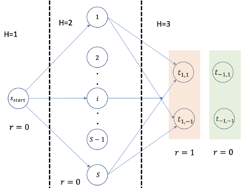
(a) Illustration of the $3$-stage, single action MDP. Each state can be visited for at most one $h=1,2,3$. $r$ is the reward for each state.(action omitted since there’s only one)

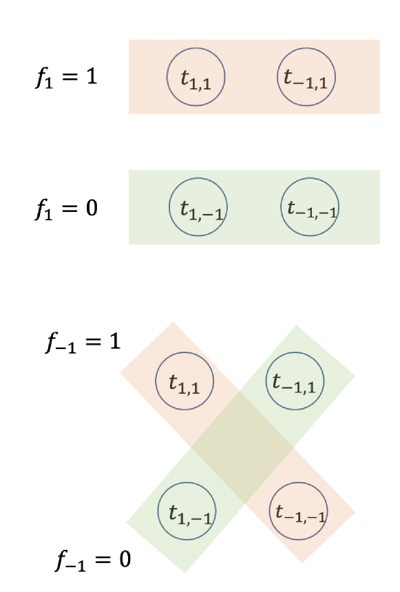
(b) Illustration of $f_{1}$ and $f_{-1}$. They only differ on $t_{-1,1}$ and $t_{-1,-1}$. For $h=3$, the Bellman error $\|{f_{c^{\prime}}-\mathcal{T}^{3}_{c,{\bm{\sigma}}}f_{c^{\prime}}}\|_{2,\mu_{3}}^{2}=0.5$, regardless of $c^{\prime}$ and $c$.

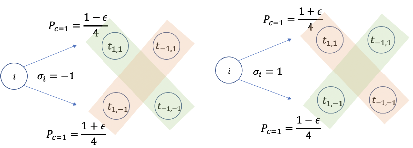
(c) Illustration of $\overline{\mathbb{P}}^{\varepsilon}_{1,\sigma_{i}}$. When $c=1$, there are two different but equally likely types of state $i$, depending on their probability transition matrix for the next step.

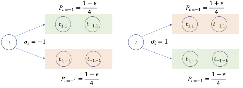
(d) Illustration of $\overline{\mathbb{P}}^{\varepsilon}_{-1,\sigma_{i}}$. When $c=1$, there are two different but equally likely types of state $i$, depending on their probability transition matrix for the next step.

Figure 1: Graphical illustration of the hard instances $\mathcal{M}^{\varepsilon}_{c,{\bm{\sigma}}}$. As shown in Equation 65, the total Bellman error is only determined by the Bellman error for $h=2$, which is equal to optimal error + $\frac{\varepsilon^{2}}{12}\mathds{1}\left[c\neq c^{\prime}\right]$ if $f_{c^{\prime}}$ is the returned function. The main idea of the proof is to show it’s difficult to guess $c$ via the observed dataset $D$ if $D$ only contains single-sampled data. As a sanity check, for any $c$ and sample $(i,t_{j,k})$, if $\sigma_{i}\overset{unif}{\sim}\{\pm 1\}$, the marginal distribution of $t_{j,k}$ is always uniform, but for double sampling of form $(i,t_{j,k},t_{j^{\prime},k^{\prime}})$, we can decide $c$ by simply looking at histogram of $(t_{j,k},t_{j^{\prime},k^{\prime}})$.

Function class:

$\mathcal{F}=\{f_{1},f_{-1}\}$, where $f_{c}(s_{\text{start}})=\frac{1}{2}$, $f_{c}(i)=\frac{1}{2},\forall 1\leq i\leq S$ and $f_{c}(t_{j,k})=\frac{k\max(c,j)+1}{2}$, $\forall c,j,k\in\{\pm 1\}$. Compared to the notation in the main paper, we drop the dependency on $h$ for $f\in\mathcal{F}$. This is because the MDP will reach a disjoint set of states for each step $h$ (see below).

Probability Transition Matrix:

We define the probability transition matrix below. Specifically, for $i\in\{1,\ldots,S\}$ and $j,k\in\{\pm 1\}$, $\mathbb{P}^{\varepsilon}_{c,{\bm{\sigma}}}(t_{j,k}\mid i)\equiv\overline{\mathbb{P}}^{\varepsilon}_{c,\sigma_{i}}(t_{j,k}):=0.25(1+\varepsilon k\max(-c,j)\sigma_{i}).$

	$s_{\text{start}}$	$i(i=1,\ldots,S)$	$t_{j,k}$	$s_{\text{end}}$
$s_{\text{start}}$	0	$\frac{1}{S}$	0	0
$i(i=1,\ldots,S)$	0	0	$\overline{\mathbb{P}}^{\varepsilon}_{c,\sigma_{i}}(t_{j,k}):=0.25(1+\varepsilon k\max(-c,j)\sigma_{i})$	0
$t_{j,k}$	$0$	$0$	$0$	1

Table 1: Probability Transition Matrix $\mathbb{P}^{\varepsilon}_{c,{\bm{\sigma}}}$ for MDP $\mathcal{M}^{\varepsilon}_{c,{\bm{\sigma}}}$. Starting from $s_{\text{start}}$, the process terminates as it reaches $s_{\text{end}}$ in the $4$th step.

Reward Function:

$r(s_{\text{start}})=0,r(i)=0,\forall 1\leq i\leq S$, $r(t_{j,k})=\frac{j+1}{2},\forall j,k\in\{-1,1\}$.

Underlying distribution:

We define the underlying distribution for batch data $\mu$ as $\mu_{2}(i)=\frac{1}{S}$ and $\mu_{3}(t_{j,k})=\frac{1}{4}$, we can check that 1 is satisfied with $C=2$ as $\varepsilon<0.5$. Define $\mathcal{T}^{1}_{c,{\bm{\sigma}}},\mathcal{T}^{2}_{c,{\bm{\sigma}}},\mathcal{T}^{3}_{c,{\bm{\sigma}}}$ be the Bellman operator of $\mathcal{M}^{\varepsilon}_{c,\sigma}$, we have $\forall{\bm{\sigma}}\in\{-1,1\}^{S}$, $\forall c,c^{\prime}\in\{-1,1\}$,

$$\|{f_{c^{\prime}}-\mathcal{T}^{3}_{c,{\bm{\sigma}}}f_{c^{\prime}}}\|_{2,\mu_{3}}^{2}=\|{f_{c^{\prime}}-r}\|_{2,\mu_{3}}^{2}=\mathop{\mathbb{missing}}{P}\left[j\neq k\max(c^{\prime},j)\right]=0.5,$$

$$\|{f_{c^{\prime}}-\mathcal{T}^{2}_{c,{\bm{\sigma}}}f_{c^{\prime}}}\|_{2,\mu_{2}}^{2}= \Bigg{\|}\sum_{j,k\in\{\pm 1\}}\mathbb{P}_{c,{\bm{\sigma}}}(t_{j,k}\mid i)f_{c^{\prime}}(t_{j,k})\Bigg{\|}_{2,\mu_{2}}^{2}$$

$$= \frac{1}{64}\bigg{\|}\sum_{j,k}\varepsilon\sigma_{i}k^{2}\max(j,c)\max(j,-c^{\prime})\bigg{\|}_{2,\mu_{2}}^{2}=\frac{\varepsilon^{2}}{4}\mathds{1}\left[c\neq c^{\prime}\right],$$

$$\|{f_{c^{\prime}}-\mathcal{T}^{1}_{c,{\bm{\sigma}}}f_{c^{\prime}}}\|_{2,\mu_{3}}^{2}=\|{f_{c}(s_{\text{start}})-f_{c}(i)}\|_{2,\mu_{1}}^{2}=0.$$

Thus

$$\mathcal{E}_{c,{\bm{\sigma}}}(f_{c^{\prime}})\equiv\mathcal{E}_{\mathcal{M}_{c,{\bm{\sigma}}}}(f_{c^{\prime}})=\frac{1}{3}\sum_{h=1}^{3}\|{f_{c^{\prime}}-\mathcal{T}^{h}_{c,{\bm{\sigma}}}f_{c^{\prime}}}\|_{2,\mu_{h}}^{2}=\frac{1}{3}(0.5+\frac{\varepsilon^{2}}{4}\mathds{1}\left[c\neq c^{\prime}\right]).$$ (65)

From eq. 65 we can see minimizing Bellman error in this case is equivalent to predict $-c$. And any algorithm predicts $c$ wrongly, i.e., outputs $f_{c^{\prime}}$ with $c^{\prime}\neq c$ with constant probability, will suffer $\Omega(\varepsilon^{2})$ expected optimality gap. More specifically, we can show that for random ${\bm{\sigma}}$, it’s information-theoretically hard to predict $c$ correctly given $D$, which leads to the following theorem.

Theorem E.2.

For $c\overset{iid}{\sim}\{-1,1\}$, ${\bm{\sigma}}\overset{iid}{\sim}\{-1,1\}^{S}$, $D=\cup_{h=1}^{3}\{(s_{i},a_{i},r_{i},s^{\prime}_{i},h)\}_{i=1}^{n}$ sampled from $\mathcal{M}^{\varepsilon}_{c,{\bm{\sigma}}}$ and $\mu$, we have for any learning algorithm $\mathfrak{A}$ with $n=O(\frac{\sqrt{S}}{\varepsilon^{2}})$ samples,

$$\mathbb{E}_{c,{\bm{\sigma}}}\mathbb{E}_{D}\left[\mathcal{E}_{c,{\bm{\sigma}}}\left(\mathfrak{A}(D)\right)\right]\geq\mathbb{E}_{c,{\bm{\sigma}}}\left[\min_{c^{\prime}\in\{-1,1\}}\mathcal{E}_{c,{\bm{\sigma}}}\left(f_{c^{\prime}}\right)\right]+\Omega(\varepsilon^{2}).$$

Or equivalently (and more specifically), if we view $\widetilde{\mathfrak{A}}(D)$ as the modified version of $\mathfrak{A}$, whose range is $\{-1,1\}$ and satisfies $\mathfrak{A}=f_{c}$ with $c=\widetilde{\mathfrak{A}}(D)$. Then we have

$$\mathbb{E}_{c,{\bm{\sigma}}}\mathbb{E}_{D}\left[\mathds{1}\left[\widetilde{\mathfrak{A}}(D)\neq c\right]\right]\geq\Omega(\varepsilon^{2}).$$

Towards proving Theorem E.2, we need the following lower bound, where $\mu_{2}\circ\mathbb{P}^{\varepsilon}_{c,{\bm{\sigma}}}$ is defined as the joint distribution of $(s,s^{\prime})$, where $s\sim\mu_{2}$ and $s^{\prime}\sim\mathbb{P}_{c,{\bm{\sigma}}|s}$. Note that when $\varepsilon=0$, $\mathbb{P}^{0}_{c,{\bm{\sigma}}}(\cdot\mid i)$ becomes uniform distribution for every $1\leq i\leq S$, and thus is independent of $c,{\bm{\sigma}}$, which could be denoted by $\mathbb{P}^{0}$ therefore.

Lemma E.3.

If $n\leq 0.1\frac{S^{0.5}}{\varepsilon^{2}}$, then $\|{\mathbb{E}_{{\bm{\sigma}}}\left(\mu_{2}\circ\mathbb{P}^{\varepsilon}_{c,{\bm{\sigma}}}\right)^{n}-\left(\mu_{2}\circ\mathbb{P}^{0}\right)^{n}}\|_{TV}\leq 0.1$, for all $c\in\{-1,1\}$.

Proof.

For convenience, we denote $\left(\mu_{2}\circ\mathbb{P}^{0}\right)^{n}$ by $P$ and $\mathbb{E}_{{\bm{\sigma}}}\left(\mu_{2}\circ\mathbb{P}^{\varepsilon}_{c,{\bm{\sigma}}}\right)^{n}$ by $Q$. By Pinsker’s inequality, we have $\|{P-Q}\|_{TV}\leq\sqrt{2KL(P,Q)}$, for any distribution $P,Q$. Thus it suffices to upper bound $KL(P,Q)$ by $0.05$.

We define $E_{i}$ as a random subset, i.e., $E_{i}=\{l|1\leq l\leq n,s_{l}=i\}$, given $D=\{(s_{i},s_{i}^{\prime})\}_{i=1}^{n}$. Then for both $\mathbb{E}_{{\bm{\sigma}}}\left(\mu_{2}\circ\mathbb{P}^{\varepsilon}_{c,{\bm{\sigma}}}\right)^{n}$ and $\left(\mu_{2}\circ\mathbb{P}^{0}\right)^{n}$, $s_{1},\ldots,s_{n}$ are i.i.d. distributed by $\mu_{2}$. Note that

$$\begin{split}&Q(s^{\prime}_{1},\ldots,s^{\prime}_{n}\mid s_{1},\ldots,s_{n})\\ =&\sum_{{\bm{\sigma}}\in\{-1,1\}^{S}}p({\bm{\sigma}})Q(s^{\prime}_{1},\ldots,s^{\prime}_{n}\mid s_{1},\ldots,s_{n},{\bm{\sigma}})\\ =&\sum_{{\bm{\sigma}}\in\{-1,1\}^{S}}\prod_{i=1}^{S}p(\sigma_{i})\prod_{i=1}^{S}Q(s^{\prime}_{E_{i}}|E_{i},\sigma_{i})\\ =&\prod_{i=1}^{S}\left(\sum_{\sigma_{i}\in\{-1,1\}}p(\sigma_{i})Q(s^{\prime}_{E_{i}}|E_{i},\sigma_{i})\right),\end{split}$$ (66)

and

$$\begin{split}P(s^{\prime}_{1},\ldots,s^{\prime}_{n}\mid s_{1},\ldots,s_{n})=\prod_{i=1}^{S}P(s^{\prime}_{E_{i}}|E_{i}).\\ \end{split}$$ (67)

For any tuple $(s_{1},\ldots,s_{n})$ and subset $E\subset\{1,\ldots,n\}$, we define $s_{E}$ as the sub-tuple of $s$ with length $|E|$ selected by $E$. Define $P_{E_{i}},Q_{E_{i}}$ as the distribution of $s^{\prime}_{E_{i}}$ conditioned on $E_{i}$. In detail, $Q_{E_{i}}(s^{\prime}_{E_{i}})=\sum\limits_{\sigma_{i}\in\{-1,1\}}p(\sigma_{i})Q(s^{\prime}_{E_{i}}|E_{i},\sigma_{i})$ and $P_{E_{i}}(s^{\prime}_{E_{i}})=P(s^{\prime}_{E_{i}}|E_{i})$. Note that for $Q$, $s^{\prime}_{E_{i}}$ are i.i.d. conditioned on $E_{i}$ and $\sigma_{i}$, i,.e., $Q(s^{\prime}_{E_{i}}|E_{i},\sigma_{i})=\prod_{l\in E_{i}}\overline{\mathbb{P}}^{\varepsilon}_{c,\sigma_{i}}(s^{\prime}_{l})$. Therefore the distribution $Q_{E_{i}}$ only depends on $|E_{i}|$, so does $P_{E_{i}}$.

Thus we can write the KL divergence as:

$$\begin{split}&KL\left(\left(\mu_{2}\circ\mathbb{P}^{0}\right)^{n},\mathbb{E}_{{\bm{\sigma}}}\left(\mu_{2}\circ\mathbb{P}^{\varepsilon}_{c,{\bm{\sigma}}}\right)^{n}\right)=KL\left(P,Q\right)=\mathop{\mathbb{missing}}{E}_{D\sim P}\left[\log\frac{P(D)}{Q(D)}\right]\\ =&\mathop{\mathbb{missing}}{E}_{D\sim P}\left[\log\frac{P(s^{\prime}_{1},\ldots,s^{\prime}_{n}\mid s_{1},\ldots,s_{n})}{Q(s^{\prime}_{1},\ldots,s^{\prime}_{n}\mid s_{1},\ldots,s_{n})}+\log\frac{P(s_{1},\ldots,s_{n})}{Q(s_{1},\ldots,s_{n})}\right]\\ =&\mathop{\mathbb{missing}}{E}_{D\sim P}\left[\log\frac{\prod_{i=1}^{S}P(s^{\prime}_{E_{i}}|E_{i})}{\prod_{i=1}^{S}Q(s^{\prime}_{E_{i}}|E_{i})}+\log\frac{P(s_{1},\ldots,s_{n})}{Q(s_{1},\ldots,s_{n})}\right]\quad(P(s_{1},\ldots,s_{n})=Q(s_{1},\ldots,s_{n}))\\ =&\mathop{\mathbb{missing}}{E}_{D\sim P}\left[\sum_{i=1}^{S}\log\frac{P_{E_{i}}(s^{\prime}_{E_{i}})}{Q_{E_{i}}(s^{\prime}_{E_{i}})}\right]\\ =&\sum_{i=1}^{S}\mathop{\mathbb{missing}}{E}_{D\sim P}\left[\log\frac{P_{E_{i}}(s^{\prime}_{E_{i}})}{Q_{E_{i}}(s^{\prime}_{E_{i}})}\right].\\ \end{split}$$ (68)

By the definition of $P$ and $Q$, given $c\in{\pm 1}$ and $\varepsilon>0$, we can see that $\mathop{\mathbb{missing}}{E}_{D\sim P}\left[\log\frac{P_{E_{i}}(s^{\prime}_{E_{i}})}{Q_{E_{i}}(s^{\prime}_{E_{i}})}\right]$ only a function of $|E_{i}|$, and we denote it by $G_{c,\varepsilon}(|E_{i}|)$. Thus we have

$$\begin{split}&KL\left(\left(\mu_{2}\circ\mathbb{P}^{0}\right)^{n},\mathbb{E}_{{\bm{\sigma}}}\left(\mu_{2}\circ\mathbb{P}^{\varepsilon}_{c,{\bm{\sigma}}}\right)^{n}\right)\\ =&KL\left(P,Q\right)\\ =&\sum_{i=1}^{S}\sum_{m=0}^{n}\mathop{\mathbb{missing}}{E}_{D\sim P}\left[\sum_{i=1}^{S}\log\frac{P_{E_{i}}(s^{\prime}_{E_{i}})}{Q_{E_{i}}(s^{\prime}_{E_{i}})}\middle||E_{i}|=m\right]P(|E_{i}|=m)\\ =&\sum_{i=1}^{S}\sum_{m=0}^{n}G_{c,\varepsilon}(m)P(|E_{i}|=m)\\ =&S\sum_{m=0}^{n}G_{c,\varepsilon}(m)P(|E_{1}|=m).\\ \end{split}$$ (69)

The last step is because $E_{i}$ are i.i.d. distributed. For convenience, we will denote $P(|E_{1}|=m)$ by $P_{N}(m)$.

It can be shown that $G_{c,\varepsilon}(m)$ is independent of $c$, and thus we drop $c$ in the subscription. We could even simplify the expression of $G_{\varepsilon}(m)$ by defining $R_{\sigma,\varepsilon}(j)=0.5(1+j\sigma\varepsilon)$ over $\{-1,1\}$ (For $c=1$, this is effectively grouping $(t_{1,1},t_{-1,-1})$ into a state, say $1$, and $(t_{1,-1},t_{-1,1})$ into another state, say $-1$.)

$$G_{\varepsilon}(m)=KL\left(\left(\textrm{Unif}\{-1,1\}\right)^{m},\frac{\left(R^{\prime}_{-1,\varepsilon}\right)^{m}+\left(R^{\prime}_{1,\varepsilon}\right)^{m}}{2}\right).$$

Below are some basic properties of $G_{\varepsilon}(m)$.

• $G_{\varepsilon}(0)=0$.

• $G_{\varepsilon}(1)=0$.

• $G_{\varepsilon}(m)\leq\frac{6m^{2}+m}{8}\varepsilon^{4}+\frac{m}{2}\frac{\varepsilon^{4}}{1-\varepsilon^{2}}\leq 2m\varepsilon^{4}$, for $\varepsilon^{2}\leq\frac{1}{2}$.

The first two properties can be verified by direct calculation, and the third property is proved in Lemma E.4.

Now it remains to calculate $P_{N}(1)$ and $\mathop{\mathbb{missing}}{E}_{P}\left[|E_{1}|^{2}\right]$. We have

$$P_{N}(1)=n\frac{1}{S}(1-\frac{1}{S})^{n-1}\leq\frac{n}{S}(1-\frac{n}{S}),$$

and

$$\mathop{\mathbb{missing}}{E}_{P}\left[|E_{1}|^{2}\right]=\mathop{\mathbb{missing}}{E}_{P}\left[(\sum_{i=1^{n}}\mathds{1}\left[s_{i}=1\right])^{2}\right]=\mathop{\mathbb{missing}}{E}_{P}\left[\sum_{i=1}^{n}\mathds{1}\left[s_{i}=1\right]+\sum_{i,j=1,\i\neq j}^{n}\mathds{1}\left[s_{i}=s_{j}=1\right]\right]=\frac{n}{S}+\frac{n(n-1)}{S^{2}}.$$

Thus we conclude that

$$KL\left(P,Q\right)= S\sum_{m=2}^{n}P_{N}(m)G_{\varepsilon}(m)\leq S\sum_{m=2}^{n}P_{N}(m)\cdot 2m^{2}\varepsilon^{4}=2\big{(}\sum_{m=2}^{n}P_{N}(m)m^{2}\big{)}S\varepsilon^{4}$$

$$= 2\left(\mathop{\mathbb{missing}}{E}_{P}\left[|E_{1}|^{2}\right]-P_{N}(1)\right)S\varepsilon^{4}=2\left(\frac{n(n-1)}{S^{2}}+\frac{n^{2}}{S^{2}}\right)S\varepsilon^{4}\leq\frac{4n^{2}\varepsilon^{4}}{S}.$$

Since $n\leq 0.1\frac{S^{0.5}}{\varepsilon^{2}}$, we have $\|{P-Q}\|_{TV}\leq\sqrt{2KL(P,Q)}\leq\sqrt{0.08}\leq 0.1$, which completes the proof. ∎

Lemma E.4.

For $\varepsilon^{2}\leq\frac{1}{2}$, we have

$$G_{\varepsilon}(m)\leq\frac{6m^{2}+m}{8}\varepsilon^{4}+\frac{m}{2}\frac{\varepsilon^{4}}{1-\varepsilon^{2}}\leq 2m^{2}\varepsilon^{4}.$$

Proof of Lemma E.4.

Let $x_{1},\ldots,x_{n}\overset{i.i.d.}{\sim}\{-1,1\}$, we have

$$G_{\varepsilon}(m)=-\mathop{\mathbb{missing}}{E}_{{\bm{x}}}\left[\log\left(\prod_{i=1}^{m}(1-x_{i}\varepsilon)+\prod_{i=1}^{m}(1+x_{i}\varepsilon)\right)\right].$$

For convenience, we define $|{\bm{x}}|:=|\sum_{i=1}^{m}x_{i}|$. Note that

$$\prod_{i=1}^{m}(1-x_{i}\varepsilon)+\prod_{i=1}^{m}(1+x_{i}\varepsilon)=\left((1-\varepsilon)^{|{\bm{x}}|}+(1+\varepsilon)^{|{\bm{x}}|}\right)(1-\varepsilon^{2})^{\frac{m-|{\bm{x}}|}{2}}.$$

Thus

$$G_{\varepsilon}(m)=-\mathop{\mathbb{missing}}{E}_{{\bm{x}}}\left[\log\left((1-\varepsilon)^{|{\bm{x}}|}+(1+\varepsilon)^{|{\bm{x}}|}\right)\right]-\frac{m-|{\bm{x}}|}{2}\mathop{\mathbb{missing}}{E}_{{\bm{x}}}\left[\log(1-\varepsilon^{2})\right].$$

For the first term, we have

$$-\mathop{\mathbb{missing}}{E}_{{\bm{x}}}\left[\log\left((1-\varepsilon)^{|{\bm{x}}|}+(1+\varepsilon)^{|{\bm{x}}|}\right)\right]$$

$$\leq -\mathop{\mathbb{missing}}{E}_{{\bm{x}}}\left[\log\left(1+\frac{|{\bm{x}}|(|{\bm{x}}|-1)}{2}\varepsilon^{2}\right)\right]$$

$$\leq \mathop{\mathbb{missing}}{E}_{{\bm{x}}}\left[-\frac{|{\bm{x}}|(|{\bm{x}}|-1)}{2}\varepsilon^{2}+\frac{1}{2}\left(\frac{|{\bm{x}}|(|{\bm{x}}|-1)}{2}\varepsilon^{2}\right)^{2}\right]$$

$$\leq \mathop{\mathbb{missing}}{E}_{{\bm{x}}}\left[-\frac{|{\bm{x}}|(|{\bm{x}}|-1)}{2}\varepsilon^{2}+\frac{|{\bm{x}}|^{4}}{8}\varepsilon^{4}\right]$$

$$= -\frac{m}{2}\varepsilon^{2}+\mathop{\mathbb{missing}}{E}_{{\bm{x}}}\left[\frac{|{\bm{x}}|}{2}\right]\varepsilon^{2}+\frac{6m^{2}+m}{8}\varepsilon^{4}.$$

For the second term, we have

$$-\mathop{\mathbb{missing}}{E}_{{\bm{x}}}\left[\log(1-\varepsilon^{2})\right]=\mathop{\mathbb{missing}}{E}_{{\bm{x}}}\left[\log(1+\frac{\varepsilon^{2}}{1-\varepsilon^{2}})\right]\leq\frac{\varepsilon^{2}}{1-\varepsilon^{2}}=\varepsilon^{2}+\frac{\varepsilon^{4}}{1-\varepsilon^{2}}.$$

Thus $G_{\varepsilon}(m)$ only contains $\varepsilon^{4}$ terms, i.e.,

$$G_{\varepsilon}(m)\leq\frac{6m^{2}+m}{8}\varepsilon^{4}+\frac{m}{2}\frac{\varepsilon^{4}}{1-\varepsilon^{2}}\leq 2m^{2}\varepsilon^{4},$$

the last step is by assumption $\varepsilon^{2}\leq\frac{1}{2}$. ∎

Proof of Theorem E.2.

In our case, since $r$ is known and $|\mathcal{A}|=1$, we can simplify the each data in $D$ into the form of $(s,s^{\prime},h)$. Further since the probability transition matrix for $h=1$ and $h=3$ are known, below we will assume $D$ only contains $n$ pairs of $(s,s^{\prime},2)$, and we will call these states by $\{s_{i}\}_{i=1}^{n}$ and $\{s^{\prime}_{i}\}_{i=1}^{n}$. Since $\|{f_{c^{\prime}}-\mathcal{T}^{3}_{c,{\bm{\sigma}}}f_{c^{\prime}}}\|_{2,\mu_{2}}^{1}$ and $\|{f_{c^{\prime}}-\mathcal{T}^{3}_{c,{\bm{\sigma}}}f_{c^{\prime}}}\|_{2,\mu_{2}}^{1}$ are constant for all $c,c^{\prime}$, we only need to consider $\|{f_{c^{\prime}}-\mathcal{T}^{2}_{c,{\bm{\sigma}}}f_{c^{\prime}}}\|_{2,\mu_{3}}^{2}$ as our loss.

Recall we define $\mu_{2}\circ\mathbb{P}^{\varepsilon}_{c,{\bm{\sigma}}}$ as the joint distribution of $(s,s^{\prime})$, where $s\sim\mu_{2}$ and $s^{\prime}\sim\mathbb{P}_{c,{\bm{\sigma}}|s}$. Thus the dataset $D$ can be viewed as sampled from $\mathbb{E}_{c,{\bm{\sigma}}}\left(\mu_{2}\circ\mathbb{P}_{c,{\bm{\sigma}}}\right)^{n}$, i.e., $D$ is sampled from a mixture of product measures.

By Lemma E.3, we know

$$\big{\|}\mathbb{E}_{{\bm{\sigma}}}\left(\mu_{2}\circ\mathbb{P}^{\varepsilon}_{1,{\bm{\sigma}}}\right)^{n}-\mathbb{E}_{{\bm{\sigma}}}\left(\mu_{2}\circ\mathbb{P}^{\varepsilon}_{-1,{\bm{\sigma}}}\right)^{n}\big{\|}_{TV}$$

$$\leq \big{\|}\mathbb{E}_{{\bm{\sigma}}}\left(\mu_{2}\circ\mathbb{P}^{\varepsilon}_{1,{\bm{\sigma}}}\right)^{n}-\mathbb{E}_{{\bm{\sigma}}}\left(\mu_{2}\circ\mathbb{P}^{0}\right)^{n}\big{\|}_{TV}+\big{\|}\mathbb{E}_{{\bm{\sigma}}}\left(\mu_{2}\circ\mathbb{P}^{\varepsilon}_{-1,{\bm{\sigma}}}\right)^{n}-\mathbb{E}_{{\bm{\sigma}}}\left(\mu_{2}\circ\mathbb{P}^{0}\right)^{n}\big{\|}_{TV}$$

$$\leq 0.2.$$

Thus if we denote the distribution of $widetilde{\mathfrak{A}}(D)$ by $X_{c}$, where $D\sim\mathbb{E}_{{\bm{\sigma}}}\left(\mu_{2}\circ\mathbb{P}^{\varepsilon}_{c,{\bm{\sigma}}}\right)^{n}$ and ${\bm{\sigma}}\sim\{-1,1\}^{S}$, and $\widetilde{\mathfrak{A}}$ can be random, the above inequality implies $\mathop{\mathbb{missing}}{P}\left[X_{-1}\neq X_{1}\right]\leq 0.2$, and therefore we have

$$\begin{split}\mathbb{E}_{c,{\bm{\sigma}}}\mathbb{E}_{D}\left[\mathcal{E}_{c,{\bm{\sigma}}}\left(\mathfrak{A}(D)\right)\right]=&\frac{1}{2}\left(\mathbb{E}_{{\bm{\sigma}},D}\left[\mathcal{E}_{1,{\bm{\sigma}}}\left(\mathfrak{A}(D)\right)\right]+\mathbb{E}_{{\bm{\sigma}},D}\left[\mathcal{E}_{-1,{\bm{\sigma}}}\left(\mathfrak{A}(D)\right)\right]\right)\\ =&\frac{1}{6}+\frac{\varepsilon^{2}}{24}\left(\mathop{\mathbb{missing}}{P}\left[X_{1}\neq 1\right]+\mathop{\mathbb{missing}}{P}\left[X_{-1}\neq-1\right]\right)\\ =&\frac{1}{6}+\frac{\varepsilon^{2}}{24}\left(\mathop{\mathbb{missing}}{P}\left[X_{1}\neq 1\right]+\mathop{\mathbb{missing}}{P}\left[X_{-1}\neq-1\right]+\mathop{\mathbb{missing}}{P}\left[X_{1}\neq X_{-1}\right]\right)-\frac{\varepsilon^{2}}{24}\mathop{\mathbb{missing}}{P}\left[X_{1}\neq X_{-1}\right]\\ \geq&\frac{1}{6}+\frac{\varepsilon^{2}}{24}-\frac{\varepsilon^{2}}{24}\mathop{\mathbb{missing}}{P}\left[X_{1}\neq X_{-1}\right]\\ \geq&\frac{1}{6}+\frac{\varepsilon^{2}}{24}-\frac{\varepsilon^{2}}{24}\times 0.2\\ =&\frac{1}{6}+\frac{\varepsilon^{2}}{30}\\ =&\mathbb{E}_{c,{\bm{\sigma}}}\left[\min_{c^{\prime}\in\{-1,1\}}\mathcal{E}_{c,{\bm{\sigma}}}\left(f_{c^{\prime}}\right)\right]+\frac{\varepsilon^{2}}{30}.\end{split}$$ (70)

∎

E.2 Proof of Theorem E.1

Now we will prove Theorem E.1 by slightly twisting the distribution of hard instances (MDPs) constructed in the previous subsection.

Proof of Theorem E.1.

W.O.L.G, we can assume $S$ is even and $S=2S^{\prime}$ (o.w. we can just abandon one state.) The only modification from the previous lower bound with $C=2$ is now the distribution of $\sigma$ is defined as the conditional distribution of $P$ on $\sum_{i=1}^{S}=0$, i.e., $P^{\prime}({\bm{\sigma}})=P({\bm{\sigma}}|\sum_{i=1}^{S}\sigma_{i}=0)$, where $P$ is the uniform distribution on $\{-1,1\}^{S}$. The main idea is that the data distribution (i.e., distribution of $(s,s^{\prime})$) shouldn’t be very different even if we add this additional ‘balancedness’ restriction. We further define a metric $d$ on $\{-1,1\}^{S}$. In detail, for ${\bm{\sigma}},{\bm{\sigma}}^{\prime}\in\{-1,1\}^{d}$, we define $d({\bm{\sigma}},{\bm{\sigma}}^{\prime})=\frac{\sum_{i=1}^{S}|\sigma_{i}-\sigma^{\prime}_{i}|}{2S}$. We have the following lemma:

Lemma E.5.

$$W_{1}^{d}(P,P^{\prime})=\frac{1}{2S}\mathbb{E}_{P}{\left|\sum_{i=1}^{S}\sigma_{i}\right|},$$ (71)

where $W_{1}^{d}(P,P^{\prime})$ is defined as $\min\limits_{{\bm{\sigma}}\sim P,{\bm{\sigma}}^{\prime}\sim P^{\prime}}\mathbb{E}[d({\bm{\sigma}},{\bm{\sigma}}^{\prime})]$.

By Cauchy Inequality, we have

$$W_{1}^{d}(P,P^{\prime})=\frac{1}{2S}\mathbb{E}_{P}{\left|\sum_{i=1}^{S}\sigma_{i}\right|}\leq\frac{1}{2S}\sqrt{\mathbb{E}_{P}{\left(\sum_{i=1}^{S}\sigma_{i}\right)^{2}}}=\frac{1}{2\sqrt{S}}$$ (72)

Proof.

For even $S$, we define $B$ as the set of the “balanced” ${\bm{\sigma}}$, i.e., $B=\{{\bm{\sigma}}|\sum_{i=1}^{S}\sigma_{i}^{\prime}=0\}$. For every ${\bm{\sigma}}\in\{-1,1\}^{S}$, we define $Q_{\bm{\sigma}}$ as the uniform distribution on $U_{\bm{\sigma}}=\{{\bm{\sigma}}^{\prime}\mid d({\bm{\sigma}},{\bm{\sigma}}^{\prime})=\frac{|\sum_{i=1}^{S}\sigma_{i}|}{2S}\}\cap B$, i.e. ${\bm{\sigma}}^{\prime}\in U_{\bm{\sigma}}$ if and only if ${\bm{\sigma}}^{\prime}\in B$ and $d({\bm{\sigma}},{\bm{\sigma}}^{\prime})=\min_{{\bm{\sigma}}^{\prime}\in B}d({\bm{\sigma}},{\bm{\sigma}}^{\prime})$.

Now we define $\Gamma({\bm{\sigma}},{\bm{\sigma}}^{\prime})=P({\bm{\sigma}})Q_{\bm{\sigma}}({\bm{\sigma}}^{\prime})$. By definition the marginal distribution of $\Gamma$ on ${\bm{\sigma}}$ is $P$. By symmetry, the marginal distribution of ${\bm{\sigma}}^{\prime}$ is $P^{\prime}$. Thus by definition of $W_{1}$,

$$W_{1}^{d}(P,P^{\prime})\leq\mathop{\mathbb{missing}}{E}_{{\bm{\sigma}},{\bm{\sigma}}^{\prime}\sim\Gamma}\left[d({\bm{\sigma}},{\bm{\sigma}}^{\prime})\right]=\frac{1}{2S}\mathbb{E}_{P}{\left|\sum_{i=1}^{S}\sigma_{i}\right|}.$$

∎

Lemma E.6.

$$\big{\|}\left(\mu_{2}\circ\mathbb{P}^{\varepsilon}_{c,{\bm{\sigma}}}\right)^{n}-\left(\mu_{2}\circ\mathbb{P}^{\varepsilon}_{c,{\bm{\sigma}}^{\prime}}\right)^{n}\big{\|}_{TV}\leq C\varepsilon\sqrt{nd({\bm{\sigma}},{\bm{\sigma}}^{\prime})}.$$ (73)

Proof.

First, note that

$$\begin{split}&KL\left(\mu_{2}\circ\mathbb{P}^{\varepsilon}_{c,{\bm{\sigma}}},\mu_{2}\circ\mathbb{P}^{\varepsilon}_{c,{\bm{\sigma}}^{\prime}}\right)\\ =&KL\left(\mu_{2},\mu_{2}\right)+\mathop{\mathbb{missing}}{E}_{i\sim\mu_{2}}\left[KL\left(\mathbb{P}^{\varepsilon}_{c,{\bm{\sigma}}}(\cdot\mid i),\mathbb{P}^{\varepsilon}_{c,{\bm{\sigma}}^{\prime}}(\cdot\mid i)\right)\right]\\ =&0+\mathop{\mathbb{missing}}{E}_{i\sim\mu_{2}}\left[KL\left(\mathbb{P}^{\varepsilon}_{c,\sigma_{i}},\mathbb{P}^{\varepsilon}_{c,\sigma^{\prime}_{i}}\right)\right]\\ =&\mathop{\mathbb{missing}}{P}_{i\sim\mu_{2}}\left[\sigma_{i}\neq\sigma^{\prime}_{i}\right]\cdot\left(\frac{1+\varepsilon}{2}\log\frac{1+\varepsilon}{1-\varepsilon}+\frac{1-\varepsilon}{2}\log\frac{1-\varepsilon}{1+\varepsilon}\right)\\ =&\mathop{\mathbb{missing}}{P}_{i\sim\mu_{2}}\left[\sigma_{i}\neq\sigma^{\prime}_{i}\right]\cdot\varepsilon\log\frac{1+\varepsilon}{1-\varepsilon}\\ =&\mathop{\mathbb{missing}}{P}_{i\sim\mu_{2}}\left[\sigma_{i}\neq\sigma^{\prime}_{i}\right]\cdot\frac{2\varepsilon^{2}}{1-\varepsilon}\\ \leq&4d({\bm{\sigma}},{\bm{\sigma}}^{\prime})\varepsilon^{2}.\end{split}$$ (74)

Thus we have

$$\begin{split}&\big{\|}\left(\mu_{2}\circ\mathbb{P}^{\varepsilon}_{c,{\bm{\sigma}}}\right)^{n}-\left(\mu_{2}\circ\mathbb{P}^{\varepsilon}_{c,{\bm{\sigma}}^{\prime}}\right)^{n}\big{\|}_{TV}\\ \leq&\sqrt{2KL\left(\left(\mu_{2}\circ\mathbb{P}^{\varepsilon}_{c,{\bm{\sigma}}}\right)^{n},\left(\mu_{2}\circ\mathbb{P}^{\varepsilon}_{c,{\bm{\sigma}}^{\prime}}\right)^{n}\right)}\\ \leq&\sqrt{2nKL\left(\mu_{2}\circ\mathbb{P}^{\varepsilon}_{c,{\bm{\sigma}}},\mu_{2}\circ\mathbb{P}^{\varepsilon}_{c,{\bm{\sigma}}^{\prime}}\right)}\\ \leq&\varepsilon\sqrt{8md({\bm{\sigma}},{\bm{\sigma}}^{\prime})}.\end{split}$$ (75)

∎

Let $\Gamma({\bm{\sigma}},{\bm{\sigma}}^{\prime})$ be the joint probabilistic distribution on $\{-1,1\}^{S}\times\{-1,1\}^{S}$ which attains the eq. 71. Therefore the marginal distribution of $\Gamma$ is $P$ and $P^{\prime}$. And thus we have for any $c\in\{-1,1\}$,

$$\begin{split}&\|{\mathop{\mathbb{missing}}{E}_{{\bm{\sigma}}\sim P}\left[\left(\mu_{2}\circ\mathbb{P}^{\varepsilon}_{c,{\bm{\sigma}}}\right)^{n}\right]-\mathop{\mathbb{missing}}{E}_{{\bm{\sigma}}\sim P^{\prime}}\left[\left(\mu_{2}\circ\mathbb{P}^{\varepsilon}_{c,{\bm{\sigma}}^{\prime}}\right)^{n}\right]}\|_{TV}\\ \leq&\mathop{\mathbb{missing}}{E}_{{\bm{\sigma}},{\bm{\sigma}}^{\prime}\sim\Gamma}\left[\|{\left(\mu_{2}\circ\mathbb{P}^{\varepsilon}_{c,{\bm{\sigma}}}\right)^{n}-\left(\mu_{2}\circ\mathbb{P}^{\varepsilon}_{c,{\bm{\sigma}}^{\prime}}\right)^{n}}\|_{TV}\right]\\ \leq&\mathop{\mathbb{missing}}{E}_{{\bm{\sigma}},{\bm{\sigma}}^{\prime}\sim\Gamma}\left[\varepsilon\sqrt{8nd({\bm{\sigma}},{\bm{\sigma}}^{\prime})}\right]\\ \leq&\varepsilon\sqrt{n\mathop{\mathbb{missing}}{E}_{{\bm{\sigma}},{\bm{\sigma}}^{\prime}\sim\Gamma}\left[8d({\bm{\sigma}},{\bm{\sigma}}^{\prime})\right]}\\ =&\varepsilon\sqrt{8nW_{1}^{d}(P,P^{\prime})}\\ \leq&2\varepsilon n^{0.5}S^{-0.25}.\end{split}$$ (76)

Therefore, when $n\leq\frac{\sqrt{S}}{400\varepsilon^{2}}$, for any $c\in\{-1,1\}$,

$$\|{\mathop{\mathbb{missing}}{E}_{{\bm{\sigma}}\sim P}\left[\left(\mu_{2}\circ\mathbb{P}^{\varepsilon}_{c,{\bm{\sigma}}}\right)^{n}\right]-\mathop{\mathbb{missing}}{E}_{{\bm{\sigma}}\sim P^{\prime}}\left[\left(\mu_{2}\circ\mathbb{P}^{\varepsilon}_{c,{\bm{\sigma}}^{\prime}}\right)^{n}\right]}\|_{TV}\leq 0.1.$$

By Lemma E.3, we have

$$\|{\mathop{\mathbb{missing}}{E}_{{\bm{\sigma}}\sim P^{\prime}}\left[\left(\mu_{2}\circ\mathbb{P}^{\varepsilon}_{1,{\bm{\sigma}}^{\prime}}\right)^{n}\right]-\mathop{\mathbb{missing}}{E}_{{\bm{\sigma}}\sim P^{\prime}}\left[\left(\mu_{2}\circ\mathbb{P}^{\varepsilon}_{-1,{\bm{\sigma}}^{\prime}}\right)^{n}\right]}\|_{TV}\leq 0.1+0.1+0.1+0.1=0.4.$$

Thus using the same argument in eq. 70, In detail, denote the distribution of $\mathfrak{A}(D)$ by $X_{c}$, where $D\sim\mathbb{E}_{{\bm{\sigma}}}\left(\mu_{2}\circ\mathbb{P}^{\varepsilon}_{c,{\bm{\sigma}}}\right)^{n}$, ${\bm{\sigma}}\sim\{-1,1\}^{S}$, the above inequality implies $\mathop{\mathbb{missing}}{P}\left[X_{-1}\neq X_{1}\right]\leq 0.4$, and therefore we have

$$\begin{split}\mathbb{E}_{c,{\bm{\sigma}}}\mathbb{E}_{D}\left[\mathcal{E}_{c,{\bm{\sigma}}}\left(\mathfrak{A}(D)\right)\right]=&\frac{1}{2}\left(\mathbb{E}_{{\bm{\sigma}},D}\left[\mathcal{E}_{1,{\bm{\sigma}}}\left(\mathfrak{A}(D)\right)\right]+\mathbb{E}_{{\bm{\sigma}},D}\left[\mathcal{E}_{-1,{\bm{\sigma}}}\left(\mathfrak{A}(D)\right)\right]\right)\\ =&\frac{1}{6}+\frac{\varepsilon^{2}}{24}\left(\mathop{\mathbb{missing}}{P}\left[X_{1}\neq 1\right]+\mathop{\mathbb{missing}}{P}\left[X_{-1}\neq-1\right]\right)\\ =&\frac{1}{6}+\frac{\varepsilon^{2}}{24}\left(\mathop{\mathbb{missing}}{P}\left[X_{1}\neq 1\right]+\mathop{\mathbb{missing}}{P}\left[X_{-1}\neq-1\right]+\mathop{\mathbb{missing}}{P}\left[X_{1}\neq X_{-1}\right]\right)-\frac{\varepsilon^{2}}{24}\mathop{\mathbb{missing}}{P}\left[X_{1}\neq X_{-1}\right]\\ \geq&\frac{1}{6}+\frac{\varepsilon^{2}}{24}-\frac{\varepsilon^{2}}{24}\times 0.4\\ =&\frac{1}{6}+\frac{1}{40}\varepsilon^{2}\\ =&\mathbb{E}_{c,{\bm{\sigma}}}\left[\min_{c^{\prime}\in\{-1,1\}}\mathcal{E}_{c,{\bm{\sigma}}}\left(f_{c^{\prime}}\right)\right]+\frac{\varepsilon^{2}}{40}.\end{split}$$ (77)

∎

Appendix F Auxiliary Results

In this section, we prove some auxiliary lemmas. Section F.1 considers the relation between Bellman error and suboptimality in values (Lemma 3.2). Section F.2 provides a supporting lemma used in the proof of Theorem 5.5. Section F.3 presents a full version of Proposition 5.6.

F.1 Connections between Bellman error and suboptimality in value (Lemma 3.2)

In this part, we present several possible ways to connect Bellman error $\mathcal{E}(f)$ with the suboptimality gap $V_{1}^{\star}(s_{1})-V_{1}^{\pi_{f}}(s_{1})$.

Via concentrability coefficient

See 3.2

Lemma 3.2 gives a feasible method to upper bound $V_{1}^{\star}(s_{1})-V_{1}^{\pi_{f}}(s_{1})$ with $\mathcal{E}(f)$ using the concentrability coefficient introduced in 1. We provide the proof of Lemma 3.2 below.

Proof of Lemma 3.2.

The proof of Lemma 3.2 is analogous to Theorem 2 in Xie and Jiang [2020b]. We place it here for the self-containedness of our paper. In discussions below, we omit the subscript $h$ in policy $\pi_{f_{h}}$ and simply write $\pi_{f}$ to ease the notation. We first note that since $\pi_{f}$ is greedy w.r.t $f$, therefore,

$$V_{1}^{\star}(s_{1})-V_{1}^{\pi_{f}}(s_{1})\leq V_{1}^{\star}(s_{1})-f_{1}\big{(}s_{1},\pi^{\star}(s_{1})\big{)}+f_{1}\big{(}s_{1},\pi_{f}(s_{1})\big{)}-V_{1}^{\pi_{f}}(s_{1}).$$ (78)

Consider any policy $\pi$. Since $f_{H+1}=0$ and $V_{1}^{\pi}(s_{1})=\mathbb{E}\big{[}\sum_{h=1}^{H}r_{h}\,\big{|}\,s_{1},\pi\big{]}$ by definition, we have

$$f_{1}\big{(}s_{1},\pi(s_{1})\big{)}-V_{1}^{\pi}(s_{1})=\mathbb{E}\Bigg{[}\sum_{h=1}^{H}\Big{(}f_{h}(s_{h},a_{h})-\mathbb{E}_{h}^{\pi}\big{[}r_{h}+f_{h+1}\big{(}s_{h+1},a_{h+1}\big{)}\,\big{|}\,s_{h},a_{h}\big{]}\Big{)}\,\Bigg{|}\,s_{1},\pi\Bigg{]}.$$

Therefore, combined with the fact $\pi_{f}$ is the greedy policy w.r.t. $f$, we can show that

$$f_{1}\big{(}s_{1},\pi^{\star}(s_{1})\big{)}-V_{1}^{\star}(s_{1})\geq \mathbb{E}\Bigg{[}\sum_{h=1}^{H}\big{(}f_{h}-\mathcal{T}_{h}^{\star}f_{h+1}\big{)}(s_{h},a_{h})\,\Bigg{|}\,s_{1},\pi^{\star}\Bigg{]},$$ (79)

$$f_{1}(s_{1},\pi_{f}(s_{1}))-V_{1}^{\pi_{f}}(s_{1})= \mathbb{E}\Bigg{[}\sum_{h=1}^{H}\big{(}f_{h}-\mathcal{T}_{h}^{\star}f_{h+1}\big{)}(s_{h},a_{h})\,\Bigg{|}\,s_{1},\pi_{f}\Bigg{]}.$$ (80)

Plugging eqs. 79 and 80 into eq. 78 yields

$$V_{1}^{\star}(s_{1})-V_{1}^{\pi_{f}}(s_{1})\leq-\mathbb{E}\Bigg{[}\sum_{h=1}^{H}\big{(}f_{h}-\mathcal{T}_{h}^{\star}f_{h+1}\big{)}(s_{h},a_{h})\,\Bigg{|}\,s_{1},\pi^{\star}\Bigg{]}+\mathbb{E}\Bigg{[}\sum_{h=1}^{H}\big{(}f_{h}-\mathcal{T}_{h}^{\star}f_{h+1}\big{)}(s_{h},a_{h})\,\Bigg{|}\,s_{1},\pi_{f}\Bigg{]}.$$

Under 1, by Cauchy-Swartz inequality, it holds that for any policy $\pi$:

$$\Bigg{|}\mathbb{E}\Bigg{[}\sum_{h=1}^{H}\big{(}f_{h}-\mathcal{T}_{h}^{\star}f_{h+1}\big{)}(s_{h},a_{h})\,\Bigg{|}\,s_{1},\pi\Bigg{]}\Bigg{|}\leq \sqrt{H\sum_{h=1}^{H}\mathbb{E}\Bigg{[}\big{(}f_{h}-\mathcal{T}_{h}^{\star}f_{h+1}\big{)}^{2}(s_{h},a_{h})\,\Bigg{|}\,s_{1},\pi\Bigg{]}}$$

$$\leq \sqrt{C}H\sqrt{\frac{1}{H}\sum_{h=1}^{H}\big{\|}f_{h}-\mathcal{T}_{h}^{\star}f_{h+1}\big{\|}_{\mu_{h}}^{2}},$$

which finishes the proof. ∎

Via a weaker concentrability assumption

We observe that Lemma 3.2 does not necessarily need an assumption as strong as 1. In fact, the inequality $V_{1}^{\star}(s_{1})-V_{1}^{\pi_{f}}(s_{1})\leq 2H\sqrt{C\cdot\mathcal{E}(f)}$ still holds if

$$\mathbb{E}\big{[}\big{(}f_{h}-\mathcal{T}_{h}^{\star}f_{h+1}\big{)}(s_{h},a_{h})\bigm{|}s_{1},\pi\big{]}\leq\sqrt{C}\big{\|}f_{h}-\mathcal{T}_{h}^{\star}f_{h+1}\big{\|}_{\mu_{h}}\qquad\text{for $\pi=\pi^{\star}$ or $\pi=\pi_{f}$ for $f\in\mathcal{F}$}.$$ (81)

If the function class $\mathcal{F}$ and ${\mathcal{T}}^{\star}\mathcal{F}=\big{\{}{\mathcal{T}}^{\star}f=(\mathcal{T}_{1}^{\star}f_{2},\ldots,\mathcal{T}_{H}^{\star}f_{H+1})\bigm{|}f\in\mathcal{F}\big{\}}$ have good structures, we may have a tighter estimate of the required $C$. For illustrative purpose, we take a simple example where $\mathcal{F}_{h}$ is a subset of a finite dimensional linear space and $\mathcal{T}_{h}^{\star}f_{h+1}\in\mathcal{F}_{h}$ for any $f_{h+1}\in\mathcal{F}_{h+1}$. Let $\phi:\mathcal{S}\times\mathcal{A}\rightarrow\mathbb{R}^{d}$ be a basis of $\mathcal{F}_{h}$ with $\|\phi(s,a)\|_{2}\leq 1$. Define $\Sigma_{h}:=\mathbb{E}_{\mu_{h}}[\phi\phi^{\top}]\in\mathbb{R}^{d\times d}$. For any $f=w^{\top}\phi\in\mathcal{F}_{h}$, $\|f\|_{\infty}\leq\|w\|_{2}\leq\|\Sigma_{h}^{\frac{1}{2}}w\|_{2}\sqrt{1/\lambda_{\min}(\Sigma_{h})}=\|f\|_{\mu_{h}}\sqrt{1/\lambda_{\min}(\Sigma_{h})}$. Therefore, eq. 81 holds for $C=\max_{h\in[H]}\{1/\lambda_{\min}(\Sigma_{h})\}$.

F.2 Proof of Supporting Lemmas in Minimax Algorithm Analysis

Lemma F.1.

Suppose 4 holds. Denote $f^{\dagger}:=\min_{f\in\mathcal{F}}\mathcal{E}(f)$. For $h\in[H]$, it holds that

$$\big{\|}f_{h}-f^{\dagger}_{h}\big{\|}_{\rho_{h}}^{2}\leq\widetilde{C}H(H-h+1)\big{\|}\big{(}f-{\mathcal{T}}^{\star}f\big{)}-\big{(}f^{\dagger}-{\mathcal{T}}^{\star}f^{\dagger}\big{)}\big{\|}_{{\mu}}^{2}\quad\text{for $\rho_{h}=\mu_{h}$ or $\nu_{h}\times\text{Unif}(\mathcal{A})$},$$ (82)

$$\text{and}\qquad\big{\|}\mathcal{T}_{h}^{\star}f_{h+1}-\mathcal{T}_{h}^{\star}f^{\dagger}_{h+1}\big{\|}_{\mu_{h}}^{2}\leq\widetilde{C}H(H-h)\big{\|}\big{(}f-{\mathcal{T}}^{\star}f\big{)}-\big{(}f^{\dagger}-{\mathcal{T}}^{\star}f^{\dagger}\big{)}\big{\|}_{{\mu}}^{2}.$$ (83)

Proof.

1. Let $\pi_{f}$ be the greedy policy associated with $f\in\mathcal{F}$. Since $f_{H+1}=f^{\dagger}_{H+1}=0$, we have

$$f_{h}(s,a)-f^{\dagger}_{h}(s,a)= \mathbb{E}\Bigg{[}\sum_{\tau=h}^{H}\bigg{[}\Big{(}f_{\tau}\big{(}s_{\tau},a_{\tau}\big{)}-\mathbb{E}\big{[}r_{\tau}+f_{\tau+1}\big{(}s_{\tau+1},a_{\tau+1}\big{)}\,\big{|}\,s_{\tau},a_{\tau}\big{]}\Big{)}$$ (84)

$$\qquad-\Big{(}f^{\dagger}_{\tau}\big{(}s_{\tau},a_{\tau}\big{)}-\mathbb{E}\big{[}r_{\tau}+f^{\dagger}_{\tau+1}\big{(}s_{\tau+1},a_{\tau+1}\big{)}\,\big{|}\,s_{\tau},a_{\tau}\big{]}\Big{)}\bigg{]}\,\Bigg{|}\,s_{h}=s,a_{h}=a,\pi_{f}\Bigg{]}.$$

Note that

$$\mathbb{E}\big{[}r_{\tau}+f_{\tau+1}\big{(}s_{\tau+1},\pi_{f_{\tau+1}}(s_{\tau+1})\big{)}\,\big{|}\,s_{\tau},a_{\tau}\big{]}=\mathcal{T}_{\tau}^{\star}f_{\tau+1}(s_{\tau},a_{\tau}),$$ (85)

$$\mathbb{E}\big{[}r_{\tau}+f^{\dagger}_{\tau+1}\big{(}s_{\tau+1},\pi_{f_{\tau+1}}(s_{\tau+1})\big{)}\,\big{|}\,s_{\tau},a_{\tau}\big{]}\leq\mathcal{T}_{\tau}^{\star}f^{\dagger}_{\tau+1}(s_{\tau},a_{\tau}).$$

Combining eqs. 84 and 85, we learn that

$$f_{h}(s,a)-f^{\dagger}_{h}(s,a)\leq\mathbb{E}\Bigg{[}\sum_{\tau=h}^{H}\Big{[}\big{(}f_{\tau}-\mathcal{T}_{\tau}^{\star}f_{\tau+1}\big{)}-\big{(}f^{\dagger}_{\tau}-\mathcal{T}_{\tau}^{\star}f^{\dagger}_{\tau+1}\big{)}\Big{]}(s_{\tau},a_{\tau})\,\Bigg{|}\,s_{h}=s,a_{h}=a,\pi_{f}\Bigg{]}.$$ (86)

By symmetry, it also holds that

$$f^{\dagger}_{h}(s,a)-f_{h}(s,a)\leq\mathbb{E}\Bigg{[}\sum_{\tau=h}^{H}\Big{[}\big{(}f^{\dagger}_{\tau}-\mathcal{T}_{\tau}^{\star}f^{\dagger}_{\tau+1}\big{)}-\big{(}f_{\tau}-\mathcal{T}_{\tau}^{\star}f_{\tau+1}\big{)}\Big{]}(s_{\tau},a_{\tau})\,\Bigg{|}\,s_{h}=s,a_{h}=a,\pi_{f^{\dagger}}\Bigg{]}.$$ (87)

Under 4, by Cauchy-Swartz inequality, for any policy $\pi$:

$$\mathbb{E}_{(s_{h},a_{h})\sim\mu_{h}}\Bigg{(}\mathbb{E}\Bigg{[}\sum_{\tau=h}^{H}\Big{[}\big{(}f_{\tau}-\mathcal{T}_{\tau}^{\star}f_{\tau+1}\big{)}-\big{(}f^{\dagger}_{\tau}-\mathcal{T}_{\tau}^{\star}f^{\dagger}_{\tau+1}\big{)}\Big{]}(s_{\tau},a_{\tau})\,\Bigg{|}\,s_{h},a_{h},\pi\Bigg{]}\Bigg{)}^{2}$$

$$\leq (H-h+1)\mathbb{E}\Bigg{[}\sum_{\tau=h}^{H}\Big{[}\big{(}f_{\tau}-\mathcal{T}_{\tau}^{\star}f_{\tau+1}\big{)}-\big{(}f^{\dagger}_{\tau}-\mathcal{T}_{\tau}^{\star}f^{\dagger}_{\tau+1}\big{)}\Big{]}^{2}(s_{\tau},a_{\tau})\,\Bigg{|}\,(s_{h},a_{h})\sim\mu_{h},\pi\Bigg{]}$$

$$\leq \widetilde{C}(H-h+1)\sum_{\tau=h}^{H}\big{\|}\big{(}f_{\tau}-\mathcal{T}_{\tau}^{\star}f_{\tau+1}\big{)}-\big{(}f^{\dagger}_{\tau}-\mathcal{T}_{\tau}^{\star}f^{\dagger}_{\tau+1}\big{)}\big{\|}_{\mu_{\tau}}^{2}$$

$$\leq \widetilde{C}H(H-h+1)\big{\|}\big{(}f-{\mathcal{T}}^{\star}f\big{)}-\big{(}f^{\dagger}-{\mathcal{T}}^{\star}f^{\dagger}\big{)}\big{\|}_{\mu}^{2}.$$

Therefore, eqs. 86 and 87 imply eq. 82.

2. We now consider $\big{\|}\mathcal{T}_{h}^{\star}f_{h+1}-\mathcal{T}_{h}^{\star}f_{h+1}^{\dagger}\big{\|}_{\mu_{h}}$. Take $\widetilde{\pi}_{h+1}(s):=\operatorname*{arg\,max}_{a\in\mathcal{A}}\big{\{}f_{h+1}(s,a)\vee f_{h+1}^{\dagger}(s,a)\big{\}}$. Then we have

$$\big{|}V_{f_{h+1}}(s)-V_{f_{h+1}^{\dagger}}(s)\big{|}\leq\big{|}f_{h+1}\big{(}s,\widetilde{\pi}_{h+1}(s)\big{)}-f^{\dagger}_{h+1}\big{(}s,\widetilde{\pi}_{h+1}(s)\big{)}\big{|}.$$

It follows that

$$\big{\|}\mathcal{T}_{h}^{\star}f_{h+1}-\mathcal{T}_{h}^{\star}f_{h+1}^{\dagger}\big{\|}_{\mu_{h}}= \big{\|}\mathbb{E}\big{[}V_{f_{h+1}}(s^{\prime})-V_{f_{h+1}^{\dagger}}(s^{\prime})\,\big{|}\,s,a\big{]}\big{\|}_{\mu_{h}}$$

$$\leq \big{\|}V_{f_{h+1}}-V_{f_{h+1}^{\dagger}}\big{\|}_{\nu_{h}}\leq\big{\|}f_{h+1}-f_{h+1}^{\dagger}\big{\|}_{\nu_{h}\times\widetilde{\pi}_{h+1}}.$$

Similar to eqs. 86 and 87, we find that

$$\big{\|}f_{h+1}-f_{h+1}^{\dagger}\big{\|}_{\nu_{h}\times\widetilde{\pi}_{h+1}}^{2}$$

$$\leq \max_{\pi=\pi_{f}\text{ or }\pi_{f^{\dagger}}}\mathbb{E}_{(s_{h+1},a_{h+1})\sim\nu_{h}\times\widetilde{\pi}_{h+1}}\Bigg{(}\mathbb{E}\Bigg{[}\sum_{\tau=h+1}^{H}\Big{[}\big{(}f_{\tau}-\mathcal{T}_{\tau}^{\star}f_{\tau+1}\big{)}-\big{(}f^{\dagger}_{\tau}-\mathcal{T}_{\tau}^{\star}f^{\dagger}_{\tau+1}\big{)}\Big{]}(s_{\tau},a_{\tau})\,\Bigg{|}\,s_{h+1},a_{h+1},\pi\Bigg{]}\Bigg{)}^{2}$$

$$\leq (H-h)\max_{\pi=\pi_{f}\text{ or }\pi_{f^{\dagger}}}\mathbb{E}_{(s_{h+1},a_{h+1})\sim\nu_{h}\times\widetilde{\pi}_{h+1}}\mathbb{E}\Bigg{[}\sum_{\tau=h+1}^{H}\Big{[}\big{(}f_{\tau}-\mathcal{T}_{\tau}^{\star}f_{\tau+1}\big{)}-\big{(}f^{\dagger}_{\tau}-\mathcal{T}_{\tau}^{\star}f^{\dagger}_{\tau+1}\big{)}\Big{]}^{2}(s_{\tau},a_{\tau})\,\Bigg{|}\,s_{h+1},a_{h+1},\pi\Bigg{]}$$

$$\leq \widetilde{C}(H-h)\sum_{\tau=h+1}^{H}\big{\|}\big{(}f_{\tau}-\mathcal{T}_{\tau}^{\star}f_{\tau+1}\big{)}-\big{(}f^{\dagger}_{\tau}-\mathcal{T}_{\tau}^{\star}f^{\dagger}_{\tau+1}\big{)}\big{\|}_{\mu_{\tau}}^{2}\leq\widetilde{C}H(H-h)\big{\|}\big{(}f-{\mathcal{T}}^{\star}f\big{)}-\big{(}f^{\dagger}-{\mathcal{T}}^{\star}f^{\dagger}\big{)}\big{\|}_{\mu}^{2}.$$

Therefore, we conclude that $\big{\|}\mathcal{T}_{h}^{\star}f_{h+1}-\mathcal{T}_{h}^{\star}f_{h+1}^{\dagger}\big{\|}_{\mu_{h}}^{2}\leq\widetilde{C}H(H-h)\big{\|}\big{(}f-{\mathcal{T}}^{\star}f\big{)}-\big{(}f^{\dagger}-{\mathcal{T}}^{\star}f^{\dagger}\big{)}\big{\|}_{\mu}^{2}$. ∎

F.3 Proof of Proposition 5.6

Lemma F.2 (Full version of Proposition 5.6).

Let $\widetilde{\mathcal{F}}_{h+1}$ be any subset of $\mathcal{F}_{h+1}$. We have the following inequality,

$$\mathcal{R}_{n}^{\mu_{h}}\big{(}\big{\{}\mathcal{T}_{h}^{\star}f_{h+1}\,\big{|}\,f_{h+1}\in\widetilde{\mathcal{F}}_{h+1}\big{\}}\big{)}\leq\mathcal{R}_{n}^{\nu_{h}}\big{(}V_{\widetilde{\mathcal{F}}_{h+1}}\big{)}\leq\sqrt{2}A\mathcal{R}_{n}^{\nu_{h}\times\text{Unif}(\mathcal{A})}\big{(}\widetilde{\mathcal{F}}_{h+1}\big{)}.$$

Proof.

1. Due to the symmetry of Rademacher random variables,

$$\mathcal{R}_{n}^{\mu_{h}}\big{(}\big{\{}\mathcal{T}_{h}^{\star}f_{h+1}\,\big{|}\,f_{h+1}\in\widetilde{\mathcal{F}}_{h+1}\big{\}}\big{)}= \mathcal{R}_{n}^{\mu_{h}}\Big{(}\Big{\{}r_{h}+\mathbb{E}\big{[}V_{f_{h+1}}(s_{h}^{\prime})\,\big{|}\,s_{h},a_{h}\big{]}\,\Big{|}\,f_{h+1}\in\widetilde{\mathcal{F}}_{h+1}\Big{\}}\Big{)}$$

$$= \mathcal{R}_{n}^{\mu_{h}}\Big{(}\Big{\{}\mathbb{E}\big{[}V_{f_{h+1}}(s_{h}^{\prime})\,\big{|}\,s_{h},a_{h}\big{]}\,\Big{|}\,f_{h+1}\in\widetilde{\mathcal{F}}_{h+1}\Big{\}}\Big{)}.$$

By definition,

$$\mathcal{R}_{n}^{\mu_{h}}\Big{(}\Big{\{}\mathbb{E}\big{[}V_{f_{h+1}}(s_{h}^{\prime})\,\big{|}\,s_{h},a_{h}\big{]}\,\Big{|}\,f_{h+1}\in\widetilde{\mathcal{F}}_{h+1}\Big{\}}\Big{)}=\mathbb{E}_{\mu_{h}}\Bigg{[}\sup_{f_{h+1}\in\widetilde{\mathcal{F}}_{h+1}}\sum_{k=1}^{n}\sigma_{k}\mathbb{E}\big{[}V_{f_{h+1}}(s_{k,h}^{\prime})\,\big{|}\,s_{k,h},a_{k,h}\big{]}\Bigg{]}.$$

Switching the order of supremum and the inner expectation, we derive that

$$\mathcal{R}_{n}^{\mu_{h}}\Big{(}\Big{\{}\mathbb{E}\big{[}V_{f_{h+1}}(s_{h}^{\prime})\,\big{|}\,s_{h},a_{h}\big{]}\,\Big{|}\,f_{h+1}\in\widetilde{\mathcal{F}}_{h+1}\Big{\}}\Big{)}\leq\mathbb{E}\Bigg{[}\sup_{f_{h+1}\in\widetilde{\mathcal{F}}_{h+1}}\sum_{k=1}^{n}\sigma_{k}V_{f_{h+1}}(s_{k,h}^{\prime})\Bigg{]}=\mathcal{R}_{n}^{\nu_{h}}\big{(}V_{\widetilde{\mathcal{F}}_{h+1}}\big{)}.$$

2. For notational convenience, let $\mathcal{A}=[A]$. Consider a vector function $\vec{f}_{h+1}:\mathcal{S}\rightarrow\mathbb{R}^{A}$ defined as $\vec{f}_{h+1}(s):=\big{(}f_{h+1}(s,1),f_{h+1}(s,2),\ldots,f_{h+1}(s,A)\big{)}\!^{\top}\in\mathbb{R}^{A}$. Then for any $f_{h+1},f^{\prime}_{h+1}\in\mathcal{F}_{h+1}$, $\big{|}V_{f_{h+1}}(s)-V_{f^{\prime}_{h+1}}(s)\big{|}\leq\|\vec{f}_{h+1}-\vec{f}^{\prime}_{h+1}\|_{\infty}\leq\|\vec{f}_{h+1}-\vec{f}^{\prime}_{h+1}\|_{2}$, i.e. the mapping $\mathbb{R}^{A}\ni\vec{f}_{h+1}(s)\mapsto V_{f_{h+1}}(s)$ is $1$-Lipschitz. By Lemma G.7, we have

$$\mathcal{R}_{n}^{\nu_{h}}\big{(}V_{\widetilde{\mathcal{F}}_{h+1}}\big{)}\leq\sqrt{2}\mathbb{E}\Bigg{[}\sup_{f_{h+1}\in\widetilde{\mathcal{F}}_{h+1}}\sum_{k=1}^{n}\sum_{a\in\mathcal{A}}\sigma_{k,a}f_{h+1}(s_{k}^{\prime},a)\Bigg{]},$$

where $s_{1}^{\prime},s_{2}^{\prime},\ldots,s_{n}^{\prime}$ are i.i.d. samples generated from $\nu_{h}$. Let $a_{1}^{\prime},a_{2}^{\prime},\ldots,a_{n}^{\prime}\in\mathcal{A}$ be random variables such that $\mathbb{P}(a_{k}^{\prime}=a\,|\,s_{k}^{\prime})=A^{-1}$ for $a\in\mathcal{A}$. It follows that

$$\mathbb{E}\Bigg{[}\sup_{f_{h+1}\in\widetilde{\mathcal{F}}_{h+1}}\sum_{k=1}^{n}\sum_{a\in\mathcal{A}}\sigma_{k,a}f_{h+1}(s_{k}^{\prime},a)\Bigg{]}\leq A\mathbb{E}\Bigg{[}\frac{1}{A}\sum_{a\in\mathcal{A}}\sup_{f_{h+1}\in\widetilde{\mathcal{F}}_{h+1}}\sum_{k=1}^{n}\sigma_{k,a}f_{h+1}(s_{k}^{\prime},a)\Bigg{]}$$

$$= A\mathbb{E}\Bigg{[}\sup_{f_{h+1}\in\widetilde{\mathcal{F}}_{h+1}}\sum_{k=1}^{n}\sigma_{k,a_{k}^{\prime}}f_{h+1}(s_{k}^{\prime},a_{k}^{\prime})\Bigg{]}=A\mathcal{R}_{n}^{\nu_{h}\times\text{Unif}(\mathcal{A})}\big{(}\widetilde{\mathcal{F}}_{h+1}\big{)}.$$

Therefore, $\mathcal{R}_{n}^{\nu_{h}}\big{(}V_{\widetilde{\mathcal{F}}_{h+1}}\big{)}\leq\sqrt{2}A\mathcal{R}_{n}^{\nu_{h}\times\text{Unif}(\mathcal{A})}\big{(}\widetilde{\mathcal{F}}_{h+1}\big{)}$. ∎

Appendix G Useful Results for (Local) Rademacher Complexity

In this section, we sumarize some useful results for (local) Rademacher complexity that are used throughout our analysis.

G.1 Concentration with Rademacher Complexity

Lemma G.1 below shows some uniform concentration inequalities with Rademacher complexity.

Lemma G.1.

Let $\mathcal{F}$ be a class of functions with ranges in $[a,b]$. With probability at least $1-\delta$,

$$Pf\leq P_{n}f+2\mathcal{R}_{n}(\mathcal{F})+(b-a)\sqrt{\frac{2\log(2/\delta)}{n}},\qquad\text{for any $f\in\mathcal{F}$}.$$

Also, with probability at least $1-\delta$,

$$P_{n}f\leq Pf+2\mathcal{R}_{n}(\mathcal{F})+(b-a)\sqrt{\frac{2\log(2/\delta)}{n}},\qquad\text{for any $f\in\mathcal{F}$}.$$

Proof.

Consider the empirical process $\sup_{f\in\mathcal{F}}(Pf-P_{n}f)$. By McDiarmid’s inequality, with probability at least $1-\delta$,

$$\sup_{f\in\mathcal{F}}\big{(}Pf-P_{n}f\big{)}\leq\mathbb{E}\sup_{f\in\mathcal{F}}\big{(}Pf-P_{n}f\big{)}+(b-a)\sqrt{\frac{2\log(2/\delta)}{n}}.$$ (88)

The basic property of Rademacher complexity ensures that

$$\mathbb{E}\sup_{f\in\mathcal{F}}\big{(}Pf-P_{n}f\big{)}\leq 2\mathcal{R}_{n}(\mathcal{F}).$$ (89)

Combining eqs. 88 and 89, we finish the proof. ∎

G.2 Concentration with Local Rademacher complexity

In this part, we present some auxiliary results regarding local Rademacher complexity. In particular, Lemma G.2 guarantees the well-definedness of critical radius, Theorem G.3 provides concentration inequalities and Lemma G.5 gives some useful properties of sub-root functions.

G.2.1 Well-definedness of critical radius

Recall that in Definition 2.3, the critical radius $r^{\star}$ of local Rademacher complexity $\mathcal{R}_{n}^{\rho}(\{f\in\mathcal{F}\mid T(f)\leq r\})$ is defined as the possitive fixed point of some sub-root functions $\psi(r)$. The following Lemma G.2 ensures that $r^{\star}$ exists and is unique.

Lemma G.2 (Lemma 3.2 in Bartlett et al. [2005]).

If $\psi:[0,\infty)\rightarrow[0,\infty)$ is a nontrivial sub-root function, then it is continuous on $[0,\infty)$ and the equation $\psi(r)=r$ has a unique positive solution $r^{\star}$. Moreover, for all $r>0$, $r\geq\psi(r)$ if and only if $r^{\star}\leq r$.

G.2.2 Concentration inequalities

Throughout the paper, we use Theorem G.3 below to prove uniform concentration with local Rademacher complexity. Theorem G.3 is a variant of Theorem 3.3 in Bartlett et al. [2005].

Theorem G.3 (Corollary of Theorem 3.3 in Bartlett et al. [2005]).

Let $\mathcal{F}$ be a class of functions with ranges in $[a,b]$ and assume that there are some functional $T:\mathcal{F}\rightarrow\mathbb{R}^{+}$ and some constants $B$ and $\eta$ such that for every $f\in\mathcal{F}$, ${\rm Var}[f]\leq T(f)\leq B(Pf+\eta)$. Let $\psi$ be a sub-root function and let $r^{\star}$ be the fixed point of $\psi$. Assume that $\psi$ satisfies, for any $r\geq r^{\star}$, $\psi(r)\geq B\mathcal{R}_{n}\big{(}\big{\{}f\in\mathcal{F}\,\big{|}\,T(f)\leq r\big{\}}\big{)}$. Then for any $\theta>1$, with probability at least $1-\delta$,

$$Pf\leq\frac{\theta}{\theta-1}P_{n}f+\frac{c_{1}\theta}{B}r^{\star}+\big{(}c_{2}(b-a)+c_{3}B\theta\big{)}\frac{\log(1/\delta)}{n}+\frac{\eta}{\theta-1},\qquad\text{for any $f\in\mathcal{F}$}.$$ (90)

Also, with probability at least $1-\delta$,

$$P_{n}f\leq\frac{\theta+1}{\theta}Pf+\frac{c_{1}\theta}{B}r^{\star}+\big{(}c_{2}(b-a)+c_{3}B\theta\big{)}\frac{\log(1/\delta)}{n}+\frac{\eta}{\theta},\qquad\text{for any $f\in\mathcal{F}$}.$$

Here, $c_{1},c_{2},c_{3}>0$ are some universal constants.

Proof.

Theorem G.3 is proved in the same way as the first part of Theorem 3.3 in Bartlett et al. [2005], by applying the following Lemma G.4 instead of Lemma 3.8 in Bartlett et al. [2005]. ∎

Given a class $\mathcal{F}$, $\lambda>1$ and $r>0$, let $w(f):=\min\big{\{}r\lambda^{k}\,\big{|}\,k\in\mathbb{N},r\lambda^{k}\geq T(f)\big{\}}$ and set $\mathcal{G}_{r}:=\big{\{}\frac{r}{w(f)}f\,\big{|}\,f\in\mathcal{F}\big{\}}$. Define $V_{r}^{+}:=\sup_{g\in\mathcal{G}_{r}}Pg-P_{n}g$ and $V_{r}^{-}:=\sup_{g\in\mathcal{G}_{r}}P_{n}g-Pg$.

Lemma G.4 (Corollary of Lemma 3.8 in Bartlett et al. [2005]).

Assume that there is a constant $B>0$ such that for every $f\in\mathcal{F}$, $T(f)\leq B(Pf+\eta)$. Fix $\theta>1$, $\lambda>0$ and $r>0$. If $V_{r}^{+}\leq\frac{r}{\lambda B\theta}$, then $Pf\leq\frac{\theta}{\theta-1}P_{n}f+\frac{r}{\lambda B\theta}+\frac{\eta}{\theta-1}$. Also, if $V_{r}^{-}\leq\frac{r}{\lambda B\theta}$, then $P_{n}f\leq\frac{\theta+1}{\theta}Pf+\frac{r}{\lambda B\theta}+\frac{\eta}{\theta}$.

Proof.

When $V_{r}^{+}\leq\frac{r}{\lambda B\theta}$, following the same reasoning as Lemma 3.8 in Bartlett et al. [2005], we derive that $Pf\leq P_{n}f+\theta^{-1}(Pf+\eta)$ under the modified condition $T(f)\leq B(Pf+\eta)$. It immediately implies the first statement. Similarly, the second part is proved by showing that $P_{n}f\leq Pf+\theta^{-1}(Pf+\eta)$. ∎

G.2.3 Properties of sub-root functions

We apply the following Lemma G.5 to simplify the forms of critical radii.

Lemma G.5.

If $\psi\!:\![0,\infty)\!\rightarrow\![0,\infty)$ is a nontrivial sub-root function and $r^{\star}$ is its positive fixed point, then

1. $\psi(r)\leq\sqrt{r^{\star}r}$ for any $r\geq r^{\star}$.

2. For any $c>0$, $\widetilde{\psi}(r):=c\psi(c^{-1}r)$ is sub-root and its positive fixed point $\widetilde{r}^{\star}$ satisfies $\widetilde{r}^{\star}=cr^{\star}$.

3. For any $C>0$, $\widetilde{\psi}(r):=C\psi(r)$ is sub-root and its positive fixed point $\widetilde{r}^{\star}$ satisfies $\widetilde{r}^{\star}\leq(C^{2}\vee 1)r^{\star}$.

4. For any $\Delta r\!>\!0$, $\widetilde{\psi}(r):=\psi(r\!+\!\Delta r)$ is sub-root and its positive fixed point $\widetilde{r}^{\star}$ satisfies $\widetilde{r}^{\star}\!\leq\!r^{\star}\!+\!\sqrt{r^{\star}\Delta r}$.

If $\psi_{i}\!\!:\!\![0,\infty)\!\rightarrow\![0,\infty)$, $\!i\!=\!\!1,...,\!n$ are nontrivial sub-root functions and $r_{i}^{\star}\!$ is the positive fixed point of $\psi_{i}$, then

1. $\widetilde{\psi}(r)=\sum_{i=1}^{n}\psi_{i}(r)$ is sub-root and its positive fixed point $\widetilde{r}^{\star}$ satisfies $\widetilde{r}^{\star}\leq\big{(}\sum_{i=1}^{n}\sqrt{r_{i}^{\star}}\big{)}^{2}$.

Proof.

1. Since $\psi$ is a sub-root function, we have $\frac{\psi(r)}{\sqrt{r}}\leq\frac{\psi(r^{\star})}{\sqrt{r^{\star}}}$ for any $r\geq r^{\star}$. Note that $r^{\star}>0$ is the fixed point and $\frac{\psi(r^{\star})}{\sqrt{r^{\star}}}=\sqrt{r^{\star}}$. Therefore, $\psi(r)\leq\sqrt{r^{\star}r}$ for $r\geq r^{\star}$.

2. It is evident that $\widetilde{\psi}$ is sub-root. Additionally, if $r\geq cr^{\star}$, then by Lemma G.2, we have $\widetilde{\psi}(r)=c\psi(c^{-1}r)\leq c(c^{-1}r)=r$. In contrast, if $0<r<cr^{\star}$, then $\widetilde{\psi}(r)=c\psi(c^{-1}r)>c(c^{-1}r)=r$. To this end, we can conclude that $\widetilde{r}^{\star}=cr^{\star}$.

3. We use part 1 and derive that if $\widetilde{r}^{\star}\geq r^{\star}$ then $\widetilde{r}^{\star}=\widetilde{\psi}(\widetilde{r}^{\star})=C\psi(\widetilde{r}^{\star})\leq C\sqrt{r^{\star}\widetilde{r}^{\star}}$, which further implies $\widetilde{r}^{\star}\leq C^{2}r^{\star}$. Therefore, $\widetilde{r}^{\star}\leq(C^{2}\vee 1)r^{\star}$.

4. If $\widetilde{r}^{\star}+\Delta r\geq r^{\star}$, then we have $\widetilde{r}^{\star}=\widetilde{\psi}(\widetilde{r}^{\star})=\psi(\widetilde{r}^{\star}+\Delta r)\leq\sqrt{r^{\star}(\widetilde{r}^{\star}+\Delta r)}$ due to part 1. It follows that $\widetilde{r}^{\star}\leq\frac{1}{2}\big{(}r^{\star}+\sqrt{(r^{\star})^{2}+4r^{\star}\Delta r}\big{)}\leq r^{\star}+\sqrt{r^{\star}\Delta r}$.

5. If $\widetilde{r}^{\star}\geq\max_{i\in[n]}r_{i}^{\star}$, then we apply part 1 and obtain $\widetilde{r}^{\star}=\widetilde{\psi}(\widetilde{r}^{\star})=\sum_{i=1}^{n}\psi_{i}(\widetilde{r}^{\star})\leq\sum_{i=1}^{n}\sqrt{r_{i}^{\star}\widetilde{r}^{\star}}$. Hence, $\widetilde{r}^{\star}\leq\big{(}\sum_{i=1}^{n}\sqrt{r_{i}^{\star}}\big{)}^{2}$. ∎

G.3 Contraction property of Rademacher complexity

Our analyses use contraction properties of Rademacher complexity. See Lemmas G.6 and G.7.

Lemma G.6 (Contraction property of Rademacher complexity, Ledoux and Talagrand [2013], Theorem A.6 in Bartlett et al. [2005]).

Suppose $\mathcal{F}\subseteq\{f:\mathcal{X}\rightarrow\mathbb{R}\}$. Let $\phi:\mathbb{R}\rightarrow\mathbb{R}$ be a contraction such that $|\phi(x)-\phi(y)|\leq|y-y^{\prime}|$ for any $y,y^{\prime}\in\mathbb{R}$. Then for any $X_{1},X_{2},\ldots,X_{n}\in\mathcal{X}$,

$$\widehat{\mathcal{R}}_{X}(\phi\circ\mathcal{F})=\mathbb{E}_{\bm{\sigma}}\bigg{[}\sup_{f\in\mathcal{F}}\frac{1}{n}\sum_{i=1}^{n}\sigma_{i}\phi\big{(}f(X_{i})\big{)}\bigg{]}\leq\mathbb{E}_{\bm{\sigma}}\bigg{[}\sup_{f\in\mathcal{F}}\frac{1}{n}\sum_{i=1}^{n}\sigma_{i}f(X_{i})\bigg{]}=\widehat{\mathcal{R}}_{X}(\mathcal{F}).$$

Lemma G.7 (Vector-form contraction property of Rademacher complexity, Maurer [2016]).

Suppose $\bm{\mathcal{F}}$ is a collection of vector-valued functions $\bm{f}:\mathcal{X}\rightarrow\mathbb{R}^{d}$ and $h:\mathbb{R}^{d}\rightarrow\mathbb{R}$ is $L$-Lipschitz with respect to the Euclidean norm, i.e. $\big{|}h(y)-h(y^{\prime})\big{|}\leq L\|y-y^{\prime}\|_{2}$ for any $y,y^{\prime}\in\mathbb{R}^{d}$. Then for any $X_{1},X_{2},\ldots,X_{n}\in\mathcal{X}$,

$$\widehat{\mathcal{R}}_{X}(h\circ\bm{\mathcal{F}})= \mathbb{E}_{\bm{\sigma}}\bigg{[}\sup_{\bm{f}\in\bm{\mathcal{F}}}\frac{1}{n}\sum_{i=1}^{n}\sigma_{i}h\big{(}\bm{f}(X_{i})\big{)}\bigg{]}$$

$$\leq \sqrt{2}L\mathbb{E}_{\bm{\sigma}}\Bigg{[}\sup_{\bm{f}\in\bm{\mathcal{F}}}\frac{1}{n}\sum_{i=1}^{n}\sum_{j=1}^{d}\sigma_{i,j}f_{j}(X_{i})\Bigg{]}\leq\sqrt{2}L\sum_{j=1}^{d}\widehat{\mathcal{R}}_{X}\big{(}\big{\{}f_{j}\,\big{|}\,\bm{f}\in\bm{\mathcal{F}}\big{\}}\big{)}.$$

References

- Antos et al. [2008] A. Antos, C. Szepesvári, and R. Munos. Learning near-optimal policies with bellman-residual minimization based fitted policy iteration and a single sample path. Machine Learning, 71(1):89–129, 2008.
- Baird [1995] L. Baird. Residual algorithms: Reinforcement learning with function approximation. In Machine Learning Proceedings 1995, pages 30–37. Elsevier, 1995.
- Baldi et al. [2001] P. Baldi, S. Brunak, and F. Bach. Bioinformatics: the machine learning approach. MIT press, 2001.
- Bartlett and Mendelson [2002] P. L. Bartlett and S. Mendelson. Rademacher and gaussian complexities: Risk bounds and structural results. Journal of Machine Learning Research, 3(Nov):463–482, 2002.
- Bartlett et al. [2005] P. L. Bartlett, O. Bousquet, S. Mendelson, et al. Local rademacher complexities. The Annals of Statistics, 33(4):1497–1537, 2005.
- Bartlett et al. [2006] P. L. Bartlett, M. I. Jordan, and J. D. McAuliffe. Convexity, classification, and risk bounds. Journal of the American Statistical Association, 101(473):138–156, 2006.
- Bertsekas and Tsitsiklis [1995] D. P. Bertsekas and J. N. Tsitsiklis. Neuro-dynamic programming: an overview. In Proceedings of 1995 34th IEEE conference on decision and control, volume 1, pages 560–564. IEEE, 1995.
- Bradtke and Barto [1996] S. J. Bradtke and A. G. Barto. Linear least-squares algorithms for temporal difference learning. Machine learning, 22(1):33–57, 1996.
- Chen and Jiang [2019] J. Chen and N. Jiang. Information-theoretic considerations in batch reinforcement learning. arXiv preprint arXiv:1905.00360, 2019.
- Cortes and Vapnik [1995] C. Cortes and V. Vapnik. Support-vector networks. Machine learning, 20(3):273–297, 1995.
- Dann et al. [2014] C. Dann, G. Neumann, J. Peters, et al. Policy evaluation with temporal differences: A survey and comparison. Journal of Machine Learning Research, 15:809–883, 2014.
- Dudley [1974] R. M. Dudley. Metric entropy of some classes of sets with differentiable boundaries. Journal of Approximation Theory, 10(3):227–236, 1974.
- Fan et al. [2020] J. Fan, Z. Wang, Y. Xie, and Z. Yang. A theoretical analysis of deep q-learning. In Learning for Dynamics and Control, pages 486–489. PMLR, 2020.
- Farahmand et al. [2008] A. M. Farahmand, M. Ghavamzadeh, C. Szepesvári, and S. Mannor. Regularized policy iteration. In nips, pages 441–448, 2008.
- Farahmand et al. [2010] A. M. Farahmand, R. Munos, and C. Szepesvári. Error propagation for approximate policy and value iteration. In Advances in Neural Information Processing Systems, 2010.
- Farahmand et al. [2016] A.-m. Farahmand, M. Ghavamzadeh, C. Szepesvári, and S. Mannor. Regularized policy iteration with nonparametric function spaces. The Journal of Machine Learning Research, 17(1):4809–4874, 2016.
- Forsyth and Ponce [2012] D. A. Forsyth and J. Ponce. Computer vision: a modern approach. Pearson,, 2012.
- Freund et al. [1996] Y. Freund, R. E. Schapire, et al. Experiments with a new boosting algorithm. In icml, volume 96, pages 148–156. Citeseer, 1996.
- Hastie et al. [2009] T. Hastie, R. Tibshirani, and J. Friedman. The elements of statistical learning: data mining, inference, and prediction. Springer Science & Business Media, 2009.
- James et al. [2013] G. James, D. Witten, T. Hastie, and R. Tibshirani. An introduction to statistical learning, volume 112. Springer, 2013.
- Jelinek [1997] F. Jelinek. Statistical methods for speech recognition. MIT press, 1997.
- Jiang et al. [2017] N. Jiang, A. Krishnamurthy, A. Agarwal, J. Langford, and R. E. Schapire. Contextual decision processes with low bellman rank are pac-learnable. In Proceedings of the 34th International Conference on Machine Learning-Volume 70, pages 1704–1713. JMLR. org, 2017.
- Juang and Rabiner [1991] B. H. Juang and L. R. Rabiner. Hidden markov models for speech recognition. Technometrics, 33(3):251–272, 1991.
- Kallus and Uehara [2020] N. Kallus and M. Uehara. Double reinforcement learning for efficient off-policy evaluation in markov decision processes. Journal of Machine Learning Research, 21(167):1–63, 2020.
- Lange et al. [2012] S. Lange, T. Gabel, and M. Riedmiller. Batch reinforcement learning. In Reinforcement learning, pages 45–73. Springer, 2012.
- Lazaric et al. [2012] A. Lazaric, M. Ghavamzadeh, and R. Munos. Finite-sample analysis of least-squares policy iteration. Journal of Machine Learning Research, 13:3041–3074, 2012.
- Le et al. [2019] H. Le, C. Voloshin, and Y. Yue. Batch policy learning under constraints. In International Conference on Machine Learning, pages 3703–3712. PMLR, 2019.
- Ledoux and Talagrand [2013] M. Ledoux and M. Talagrand. Probability in Banach Spaces: isoperimetry and processes. Springer Science & Business Media, 2013.
- Levine et al. [2020] S. Levine, A. Kumar, G. Tucker, and J. Fu. Offline reinforcement learning: Tutorial, review, and perspectives on open problems. arXiv preprint arXiv:2005.01643, 2020.
- Maurer [2016] A. Maurer. A vector-contraction inequality for rademacher complexities. In International Conference on Algorithmic Learning Theory, pages 3–17. Springer, 2016.
- Mendelson [2002] S. Mendelson. Geometric parameters of kernel machines. In International Conference on Computational Learning Theory, pages 29–43. Springer, 2002.
- Mnih et al. [2015] V. Mnih, K. Kavukcuoglu, D. Silver, A. A. Rusu, J. Veness, M. G. Bellemare, A. Graves, M. Riedmiller, A. K. Fidjeland, G. Ostrovski, et al. Human-level control through deep reinforcement learning. nature, 518(7540):529–533, 2015.
- Munos [2003] R. Munos. Error bounds for approximate policy iteration. In ICML, volume 3, pages 560–567, 2003.
- Munos [2007] R. Munos. Performance bounds in l_p-norm for approximate value iteration. SIAM journal on control and optimization, 46(2):541–561, 2007.
- Munos and Szepesvári [2008] R. Munos and C. Szepesvári. Finite-time bounds for fitted value iteration. Journal of Machine Learning Research, 9(May):815–857, 2008.
- Precup [2000] D. Precup. Eligibility traces for off-policy policy evaluation. Computer Science Department Faculty Publication Series, page 80, 2000.
- Precup et al. [2001] D. Precup, R. S. Sutton, and S. Dasgupta. Off-policy temporal-difference learning with function approximation. In ICML, pages 417–424, 2001.
- Puterman [2014] M. L. Puterman. Markov decision processes: discrete stochastic dynamic programming. John Wiley & Sons, 2014.
- Riedmiller [2005] M. Riedmiller. Neural fitted q iteration–first experiences with a data efficient neural reinforcement learning method. In European Conference on Machine Learning, pages 317–328. Springer, 2005.
- Schapire [1999] R. E. Schapire. A brief introduction to boosting. In Ijcai, volume 99, pages 1401–1406. Citeseer, 1999.
- Sun et al. [2019] W. Sun, N. Jiang, A. Krishnamurthy, A. Agarwal, and J. Langford. Model-based rl in contextual decision processes: Pac bounds and exponential improvements over model-free approaches. In Conference on Learning Theory, pages 2898–2933. PMLR, 2019.
- Sutton and Barto [2018] R. S. Sutton and A. G. Barto. Reinforcement learning: An introduction. MIT press, 2018.
- Suykens and Vandewalle [1999] J. A. Suykens and J. Vandewalle. Least squares support vector machine classifiers. Neural processing letters, 9(3):293–300, 1999.
- Szeliski [2010] R. Szeliski. Computer vision: algorithms and applications. Springer Science & Business Media, 2010.
- Uehara et al. [2020] M. Uehara, J. Huang, and N. Jiang. Minimax weight and q-function learning for off-policy evaluation. In International Conference on Machine Learning, pages 9659–9668. PMLR, 2020.
- Uehara et al. [2021] M. Uehara, M. Imaizumi, N. Jiang, N. Kallus, W. Sun, and T. Xie. Finite sample analysis of minimax offline reinforcement learning: Completeness, fast rates and first-order efficiency. arXiv preprint arXiv:2102.02981, 2021.
- van Handel [2014] R. van Handel. Probability in high dimension. Technical report, PRINCETON UNIV NJ, 2014.
- Vapnik [2013] V. Vapnik. The nature of statistical learning theory. Springer science & business media, 2013.
- Vapnik and Chervonenkis [2015] V. N. Vapnik and A. Y. Chervonenkis. On the uniform convergence of relative frequencies of events to their probabilities. In Measures of complexity, pages 11–30. Springer, 2015.
- Vershynin [2010] R. Vershynin. Introduction to the non-asymptotic analysis of random matrices. arXiv preprint arXiv:1011.3027, 2010.
- Wainwright [2019] M. J. Wainwright. High-dimensional statistics: A non-asymptotic viewpoint, volume 48. Cambridge University Press, 2019.
- Wang et al. [2020a] R. Wang, D. P. Foster, and S. M. Kakade. What are the statistical limits of offline rl with linear function approximation? arXiv preprint arXiv:2010.11895, 2020a.
- Wang et al. [2020b] R. Wang, R. R. Salakhutdinov, and L. Yang. Reinforcement learning with general value function approximation: Provably efficient approach via bounded eluder dimension. Advances in Neural Information Processing Systems, 33, 2020b.
- Xie and Jiang [2020a] T. Xie and N. Jiang. Batch value-function approximation with only realizability. arXiv preprint arXiv:2008.04990, 2020a.
- Xie and Jiang [2020b] T. Xie and N. Jiang. Q* approximation schemes for batch reinforcement learning: A theoretical comparison. arXiv preprint arXiv:2003.03924, 2020b.
- Xie et al. [2019] T. Xie, Y. Ma, and Y.-X. Wang. Towards optimal off-policy evaluation for reinforcement learning with marginalized importance sampling. arXiv preprint arXiv:1906.03393, 2019.
- Yin et al. [2020] M. Yin, Y. Bai, and Y.-X. Wang. Near optimal provable uniform convergence in off-policy evaluation for reinforcement learning. arXiv preprint arXiv:2007.03760, 2020.