Measurement Error Mitigation via Truncated Neumann Series

Abstract

Measurements on near-term quantum processors are inevitably subject to hardware imperfections that lead to readout errors. Mitigation of such unavoidable errors is crucial to better explore and extend the power of near-term quantum hardware. In this work, we propose a method to mitigate measurement errors in computing quantum expectation values using the truncated Neumann series. The essential idea is to cancel the errors by combining various noisy expectation values generated by sequential measurements determined by terms in the truncated series. We numerically test this method and find that the computation accuracy is substantially improved. Our method possesses several advantages: it does not assume any noise structure, it does not require the calibration procedure to learn the noise matrix a prior, and most importantly, the incurred error mitigation overhead is independent of system size, as long as the noise resistance of the measurement device is moderate. All these advantages empower our method as a practical measurement error mitigation method for near-term quantum devices.

I Introduction

Quantum computers hold great promise for a variety of scientific and industrial applications McArdle et al. (2020); Cerezo et al. (2020); Bharti et al. (2021); Endo et al. (2021). However, in the current stage noisy intermediate-scale quantum (NISQ) computers Preskill (2018) introduce significant errors that must be dealt with before performing any practically valuable tasks. Errors in a quantum computer are typically classified into quantum gate errors and measurement errors. For quantum gate errors, various quantum error mitigation techniques have been proposed to mitigate the damages caused by errors on near-term quantum devices Temme et al. (2017); Endo et al. (2018); Li and Benjamin (2017); McClean et al. (2017, 2020); McArdle et al. (2019); Bonet-Monroig et al. (2018); He et al. (2020); Giurgica-Tiron et al. (2020); Kandala et al. (2019); Endo et al. (2021); Sun et al. (2021); Czarnik et al. (2020). For measurement errors, experimental works have demonstrated that measurement errors in quantum devices can be well understood in terms of classical noise models Chow et al. (2012); Kandala et al. (2019); Chen et al. (2019), which is recently rigorously justified Geller (2020). Specifically, a $n$-qubit noisy measurement device can be characterized by a noise matrix $A$ of size $2^{n}\times 2^{n}$. The element in the $\bm{x}$-th row and $\bm{y}$-th column, $A_{\bm{x}\bm{y}}$, is the probability of obtaining a outcome $\bm{x}$ provided that the true outcome is $\bm{y}$. If one has access to this stochastic matrix, it is straightforward to classically reverse the noise effects simply by multiplying the probability vector obtained from experimental statistics by this matrix’s inversion. However, there are several limitations of this matrix inversion approach: (i) The complete characterization of $A$ requires $2^{n}$ calibration experiment setups and thus is not scalable. (ii) The matrix $A$ may be singular for large $n$, preventing direct inversion. (iii) The inverse $A^{-1}$ is hard to compute and might not be a stochastic matrix, indicating that it can produce negative probabilities.

Several approaches have been proposed to deal with these issues Maciejewski et al. (2020); Tannu and Qureshi (2019); Nachman et al. (2019); Hicks et al. (2021); Bravyi et al. (2020); Geller and Sun (2020); Murali et al. (2020); Kwon and Bae (2020); Funcke et al. (2020); Zheng et al. (2020); Maciejewski et al. (2021); Barron and Wood (2020). For example, Ref. Chen et al. (2019); Maciejewski et al. (2020) elucidated that the quality of the measurement calibration and the number of measurement samples affected the performance of measurement error mitigation methods dramatically. Motivated by the unfolding algorithms in high energy physic, Ref. Nachman et al. (2019); Hicks et al. (2021) used the iterative Bayesian unfolding approach to avoid pathologies from the matrix inversion. Ref. Bravyi et al. (2020) introduced a new classical noise model based on the continuous time Markov processes and proposed an error mitigation approach that cancels errors using the quasiprobability decomposition technique Pashayan et al. (2015); Temme et al. (2017); Howard and Campbell (2017); Endo et al. (2018); Takagi (2020); Jiang et al. (2020); Regula et al. (2021). However, most of these works make an explicit assumption on the physical noise model and require the calibration procedure to learn the stochastic matrix $A$, and thus is not scalable in general. Recently, Ref. Berg et al. (2020) proposed a noise model-free measurement error mitigation method that forces the bias in the expectation value to appear as a multiplicative factor that can be removed.

In this work, we propose a measurement error mitigation method motivated by the Neumann series, applicable for any quantum algorithms where the measurement statistics are used for computing the expectation values of observables. The idea behind this method is to cancel the measurement errors by utilizing the noisy expectation values generated by sequential measurements, each determined by a term in the truncated Neumann series. The method is deliberately simple, does not make any assumption about the actual physical noise model, and does not require calibrating the stochastic matrix a priori.

The paper is organized as follows. Section II describes the quantum task of computing expectation values and explains how the noisy measurement incurred bias to the results. Section III presents the error mitigation technique via truncated Neumann series. Section IV reports the experimental demonstration of our error mitigation method. The Appendices summarize technical details used in the main text.

II Computing the expectation value

Let $\rho$ be an $n$-qubit quantum state generated by a quantum circuit. Most of the quantum computing tasks end with computing the expectation value $\operatorname{Tr}[O\rho]$ of a given observable $O$ within a prefixed precision $\varepsilon$, by post-processing the measurement outcomes of the quantum state. This task is the essential component of multifarious quantum algorithms, notable practical examples of which are variational quantum eigensolvers Peruzzo et al. (2014); McClean et al. (2016), quantum approximate optimization algorithm Farhi et al. (2014), and quantum machine learning Biamonte et al. (2017); Havlíček et al. (2019).

For simplicity, we assume that the observable $O$ is diagonal in the computational basis and its elements take values in the range $[-1,1]$, i.e.,

$$O=\sum_{\bm{x}\in\{0,1\}^{n}}O(\bm{x})|{\bm{x}}\rangle\!\langle{\bm{x}}|,\quad|O(\bm{x})|\leq 1,$$ (1)

where $O(\bm{x})$ is the $\bm{x}$-th diagonal element of $O$ and $|\alpha|$ is the absolute value of $\alpha$. Note that we adopt the convention that the diagonal elements are indexed from $0$. Consider $M$ independent experiments where in each round we prepare the state $\rho$ using the same quantum circuit and measure each qubit in the computational basis (see, e.g., Fig. 1). Let $\bm{s}^{m}\in\{0,1\}^{n}$ be the measurement outcome observed in the $m$-th round. We further define the empirical mean value

$$\eta^{(0)}\mathrel{\mathop{\mathchar 58\relax}}=\frac{1}{M}\sum_{m=1}^{M}O(\bm{s}^{m}).$$ (2)

Let $\operatorname{vec}(\rho)$ be the $2^{n}$-dimensional column vector formed by the diagonal elements of $\rho$. Then Bravyi et al. (2020)

$$E^{(0)}\mathrel{\mathop{\mathchar 58\relax}}=\mathbb{E}[\eta^{(0)}]=\sum_{\bm{x}\in\{0,1\}^{n}}O(\bm{x})\langle\bm{x}|\operatorname{vec}(\rho)=\operatorname{Tr}[O\rho],$$ (3)

where $\mathbb{E}[X]$ is the expectation of the random variable $X$. Eq. (3) implies that $\eta^{(0)}$ is an unbiased estimator of $\operatorname{Tr}[O\rho]$. What’s more, the standard deviation $\sigma(\eta^{(0)})\leq 1/\sqrt{M}$. By Hoeffding’s inequality Hoeffding (1963), $M=2\log(2/\delta)/\varepsilon^{2}$ would guarantee that

$$\operatorname{Pr}\{|\eta^{(0)}-\operatorname{Tr}[O\rho]|\leq\varepsilon\}\geq 1-\delta,$$ (4)

where $\operatorname{Pr}\{\cdot\}$ is the event’s probability, $\delta$ is the specified confidence, and all logarithms are in base $2$ throughout this paper.

Figure 1: Computing the expectation value $\operatorname{Tr}[O\rho]$ with the ideal measurement device (left) and the noisy measurement device (right) not .

However, measurement devices on current quantum hardware inevitably suffer from hardware imperfections that lead to readout errors, which are manifested as a bias toward the expectation values we aim to compute (cf. the right side of Fig. 1). As previously mentioned, in the most general scenario, these errors are modeled by a $2^{n}\times 2^{n}$ noise matrix $A$. If there were no measurement error at all, $A$ is the identity matrix $I$. The off-diagonal elements of $A$ completely characterize the readout errors. By definition, $A$ is column-stochastic in the sense that the elements of each column are non-negative and sum to $1$.

Suppose now that we adopt the same procedure for computing $\eta$ in (2), where we perform $M$ independent experiments and collect the measurement outcomes. Denote by $\bm{s}^{m,1}\in\{0,1\}^{n}$ the outcome observed in the $m$-th round, where the superscript $1$ indicates that the noisy measurement is applied. As (2), we define

$$\eta^{(1)}\mathrel{\mathop{\mathchar 58\relax}}=\frac{1}{M}\sum_{m=1}^{M}O(\bm{s}^{m,1}).$$ (5)

We prove in Appendix A that

$$E^{(1)}\mathrel{\mathop{\mathchar 58\relax}}=\mathbb{E}[\eta^{(1)}]=\sum_{\bm{x}\in\{0,1\}^{n}}O(\bm{x})\langle\bm{x}|A\operatorname{vec}(\rho),$$ (6)

indicating that $\eta^{(1)}$ is no longer an estimator of $\operatorname{Tr}[O\rho]$. Comparing Eqs. (3) and (6), we find that in the ideal case, the sampled probability distribution approximates $\operatorname{vec}(\rho)$ due to the weak law of large numbers, while in the noisy case, the sampled probability distribution approximates $A\operatorname{vec}(\rho)$, leading to a bias in the estimator.

III Error mitigation via truncated Neumann series

A direct approach to eliminate the measurement errors from $A\operatorname{vec}(\rho)$ is to apply the inverse matrix $A^{-1}$. However, this approach is resource-consuming and only feasible when $n$ is small. To deal with this difficulty, we simulate the effect of $A^{-1}$ using a truncated Neumann series. That is, $A^{-1}$ is approximated by a linear combination of the terms $A^{k}$ for different $k$, with carefully chosen coefficients. This idea has previously been applied for linear data detection in massive multiuser multiple-input multiple-output wireless systems Wu et al. (2013).

Define the noise resistance of the noise matrix $A$ as

$$\xi\mathrel{\mathop{\mathchar 58\relax}}=2\left(1-\min_{\bm{x}\in\{0,1\}^{n}}\left\langle{\bm{x}}\right|A\left|{\bm{x}}\right\rangle\right).$$ (7)

By definition, $1-\xi/2$ is the minimal diagonal element of $A$. Intuitively, $\xi/2$ characterizes the noisy measurement device’s behavior in the worst-case scenario since it is the maximal probability for which the true outcome should be $\bm{x}$ yet the actual outcome is not $\bm{x}$. In the following, we assume $\xi<1$, which is equivalent to the condition that the minimal diagonal element of $A$ is larger than $0.5$. This assumption is reasonable since otherwise the measurement device is too noisy to be applied from the practical perspective. Under this assumption, the stochastic matrix $A$ is nonsingular and the Neumann series implies that (Stewart, 1998, Theorem 4.20)

$$A^{-1} =\sum_{k=0}^{\infty}(I-A)^{k}$$ (8a)

$$=\sum_{k=0}^{K}(I-A)^{k}+\mathcal{O}((I-A)^{K+1})$$ (8b)

$$=\sum_{k=0}^{K}c_{K}(k)A^{k}+\mathcal{O}((I-A)^{K+1}),$$ (8c)

where for arbitrary non-negative integers $0\leq k\leq K$, the coefficient function is defined as

$$c_{K}(k)\mathrel{\mathop{\mathchar 58\relax}}=(-1)^{k}\binom{K+1}{k+1},$$ (9)

and $\binom{n}{k}$ is the binomial coefficient. Intuitively, Eq. (8) indicates that one may approximate the inverse matrix $A^{-1}$ using the first $K$ Neumann series terms, if the behavior of the remaining terms $\mathcal{O}((I-A)^{K+1})$ can be bounded. We show that this is indeed the case in the measurement error mitigation task. More specifically, using the first $K+1$ terms in the expansion (8) of $A^{-1}$, we obtain the following.

Theorem 1.

For arbitrary positive integer $K$, it holds that

$$\left|\operatorname{Tr}[O\rho]-\sum_{k=1}^{K+1}c_{K}(k-1)E^{(k)}\right|\leq\xi^{K+1},$$ (10)

where

$$E^{(k)}\mathrel{\mathop{\mathchar 58\relax}}=\sum_{\bm{x}\in\{0,1\}^{n}}O(\bm{x})\langle\bm{x}|A^{k}\operatorname{vec}(\rho).$$ (11)

The proof is given in Appendix B. As evident from Theorem 1, the noise resistance $\xi$ of the noise matrix $A$ determines the number of terms required in the truncated Neumann series to approximate $A^{-1}$ to the desired precision. What is more, since $\xi<1$, the approximation error decays exponentially in terms of $K$. By the virtue of (6), $E^{(k)}$ can be viewed as the noisy expectation value generated by a noisy measurement device whose corresponding noise matrix is $A^{k}$. Let $\overline{E}\mathrel{\mathop{\mathchar 58\relax}}=\sum_{k=1}^{K+1}c_{K}(k-1)E^{(k)}$. Theorem 1 inspires a systematic way to estimate the expectation value $\operatorname{Tr}[O\rho]$ in two steps.

Figure 2: Experimental setup for estimating $E^{(4)}$, in which the noisy measurement device (box in blue) is executed $4$ times sequentially.

Firstly, we choose $K$ for which the RHS. of (10) evaluates to $\varepsilon$, yielding the optimal truncated number

$$K=\left\lceil\frac{\log\varepsilon}{\log\xi}-1\right\rceil.$$ (12)

Such a choice guarantees that $\overline{E}$ is $\varepsilon$-close to the expectation value $\operatorname{Tr}[O\rho]$. Secondly, we compute the quantity $\overline{E}$ by estimating each term $E^{(k)}$ and computing the linear combination according to the coefficients $c_{K}$. Since $\overline{E}$ itself is only an $\varepsilon$-estimate of $\operatorname{Tr}[O\rho]$, it suffices to approximate $\overline{E}$ within an error $\varepsilon$. Motivated by the relation between $\eta^{(1)}$ and $E^{(1)}$ (see the discussions and calculations in obtaining (5)), we declare that each $E^{(k)}$ can be estimated via the following procedure:

1. Generate a quantum state $\rho$.

2. Using $\rho$ as input, execute the noisy measurement device $k$ times sequentially and collect the outcome produced by the final measurement device, i.e., the $k$-th measurement device.

3. Repeat the above two steps $M$ rounds and collect the measurement outcomes.

4. Define an average analogous to (5) and output it as an estimate of $E^{(k)}$.

We elaborate thoroughly on the concept of sequential measurement in Appendix C and show that the classical noise model describing the sequential measurement repeating $k$ times is effectively characterized by the stochastic matrix $A^{k}$. For a sequential measurement repeating $k$ times, one can think of the rightmost $k-1$ measurements as implementing the calibration subroutine since they accept the computational basis states as inputs. To some extent, this is a dynamic calibration procedure where we do not statically enumerate all computational bases as input states but dynamically prepare the input states based on the output information of the target state from the first measurement device. For illustrative purpose, we demonstrate in Fig. 2 the experimental setup for estimating the noisy expectation value $E^{(4)}$, where the measurement device is repeated four times in each round. We summarize the whole procedure in the following Algorithm 1.

Algorithm 1 Error mitigation via truncated Neumann series

0:  Quantum circuit generating the $n$-qubit state $\rho$,      the $n$-qubit quantum observable $O$,      the $n$-qubit noisy measurement device,      noise resistance $\xi$,      probability tolerance $\delta$,      precision parameter $\varepsilon$.

0:  $\eta$, as an estimate of $\operatorname{Tr}[O\rho]$.

1:  Compute $K=\left\lceil\log\varepsilon/\log\xi-1\right\rceil$;

2:  Compute $\Delta=\binom{2K+2}{K+1}-1$;

3:  Compute $M=\lceil 2(K+1)\Delta\log(2/\delta)/\varepsilon^{2}\rceil$;

4:  for $k=1,\cdots,K+1$ do

5:     for $m=1,\cdots,M$ do

6:          Run the quantum circuit to generate $\rho$;

7:          Execute the measurement device $k$ times sequentially;

8:          Obtain the measurement outcome $\bm{s}^{m,k}$;

9:     end for

10:     Compute $\eta^{(k)}=\frac{1}{M}\sum_{m=1}^{M}O(\bm{s}^{m,k})$;

11:  end for

12:  Compute $\eta=\sum_{k=1}^{K+1}c_{K}(k-1)\eta^{(k)}$, where $c_{K}$ is defined in (9);

13:  Output $\eta$.

We claim that the output $\eta$ of Algorithm 1 approximates the expectation value $\operatorname{Tr}[O\rho]$ pretty well, as captured by the following proposition.

Proposition 2.

The output $\eta$ of Algorithm 1 satisfies

$$\operatorname{Pr}\left\{|\operatorname{Tr}[O\rho]-\eta|\leq 2\varepsilon\right\}\geq 1-\delta.$$ (13)

Proof of the proposition is given in Appendix D. Intuitively, Eq. (13) says that the output $\eta$ of Algorithm 1 estimates the ideal expectation value $\operatorname{Tr}[O\rho]$ with error $2\varepsilon$ at a probability greater than $1-\delta$. Analyzing Algorithm 1, we can see that we ought to expand the Neumann series to the $K$-th order, where $K$ is computed via (12), and estimate the $K+1$ noisy expectation values $E^{(1)},\cdots,E^{(K+1)}$ individually. For each expectation, we need $M$ copy of quantum states. As so, the total number of quantum states consumed is given by

$$M(K+1) =2(K+1)^{2}\Delta\log(2/\delta)/\varepsilon^{2}$$

$$\approx 4^{K}\log(2/\delta)/\varepsilon^{2}.$$ (14)

In other words, our error mitigation method increases the number of quantum states that is required to achieve the given precision $\varepsilon$ by a factor of $4^{K}$ compared with the case of the ideal measurement. In Fig. 3, we plot the optimal truncated number $K$ (12) as a function of the noise resistance $\xi$, the error tolerance parameter is fixed as $\varepsilon=0.01$. One can check from the figure that $K\leq 10$ whenever the noise resistance satisfies $\xi\leq 0.657$ (Equivalently, the minimal diagonal element of $A$ is larger than $0.67$). That is to say, the incurred error mitigation overhead $4^{K}$ is independent of the system size, so long as the noise resistance $\xi$ is moderate, in the sense that it is below a certain threshold (say $0.657$). On the other hand, the number of noisy quantum measurements applied in Algorithm 1 is given by

$$\left(\sum_{k=1}^{K+1}k\right)M\approx 2(K+1)^{3}\Delta\log(2/\delta)/\varepsilon^{2}.$$ (15)

Compared to (14), our method has used more number of measurements than the number of quantum states by a multiplier $K+1$. We remark that both costs are roughly characterized by the prominent factor $4^{K}$.

Figure 3: The optimal truncated number $K$ (12) as a function of the noise resistance $\xi$, where the precision parameter is $\varepsilon=0.01$.

III.1 Discussion on the noise resistance

In practical applications, $\xi$ can be obtained from the specifications of NISQ devices. For example, in IBM quantum devices, the specifications are often reported $2-10\%$ Kwon and Bae (2020). If such information is not available, we may perform calibration to obtain $A$ first and then compute $\xi$, which is still resource-efficient compared to computing the inverse matrix $A^{-1}$.

When defining $\xi$ in (7), we do not consider any structure of $A$. If certain noise model is assumed, the calculation of $\xi$ can be simplified. In the following, we consider the tensor product noise model and show that the noise resistance can be compute analytically. Assume $A$ is a tensor product of $n$ $2\times 2$ stochastic matrices, i.e.,

$$A_{\operatorname{tp}}=\begin{bmatrix}1-\alpha_{1}&\beta_{1}\\ \alpha_{1}&1-\beta_{1}\end{bmatrix}\otimes\cdots\otimes\begin{bmatrix}1-\alpha_{n}&\beta_{n}\\ \alpha_{n}&1-\beta_{n}\end{bmatrix},$$ (16)

where $\alpha_{i}$ and $\beta_{i}$ are error rates describing the $i$-th qubit’s readout errors $0\to 1$ and $1\to 0$, respectively. One can show that

$$\xi(A_{\operatorname{tp}})=2\left(1-\prod_{i=1}^{n}\min\{1-\alpha_{i},1-\beta_{i}\}\right).$$ (17)

Specially, if $\alpha_{i},\beta_{i}\ll 1$, then $\xi\approx 2(1-1/e^{\gamma})$, where $\gamma\mathrel{\mathop{\mathchar 58\relax}}=\sum_{i=1}^{n}\max\{\alpha_{i},\beta_{i}\}$ is called the noise strength in Bravyi et al. (2020).

IV Experimental results

We apply the proposed error mitigation method to the following illustrative example and demonstrate its performance. Consider the input state $\rho=|{\Phi}\rangle\!\langle{\Phi}|$, where

$$\left|{\Phi}\right\rangle\mathrel{\mathop{\mathchar 58\relax}}=\frac{1}{\sqrt{2^{n}}}\sum_{i=0}^{2^{n}-1}\left|{i}\right\rangle,$$ (18)

which is the maximal superposition state. The observable $O$ is a tensor product of Pauli $Z$ operators, i.e., $O=Z^{\otimes n}$. The ideal expectation value is $\operatorname{Tr}[O\rho]=0$. We choose $n=8$ and randomly generate a noise matrix $A^{\ast}$ whose noise resistance satisfies $\xi(A^{\ast})\approx 0.657$ (as so the noise matrix is moderate). We repeat the procedure for producing the noisy expectation value $\eta^{(1)}$ and Algorithm 1 for producing the mitigated expectation value $\eta$ a total number of $1000$ times. Note that all these experiments assume the same noise matrix $A$, and the parameters are chosen as $\varepsilon=\delta=0.01$. The obtained expectation values are scatted in Fig. 4. It is easy to see from the figure that the noisy measurement device, characterized by the noise matrix $A^{\ast}$, incurs a bias $\approx-0.007$ to the estimated expectation values. On the other hand, the error mitigated expectation values distributed evenly around the ideal value $0$ within a distance of $0.01$ with high probability. As evident from Fig. 4, several mitigated expectation values fall outside the expected region. These statistical outcomes match our conclusion in Proposition 2, validating the correctness and performance of the proposed error mitigation method.

Fig. 5 shows the (noisy and mitigated) expectation values estimated via the above procedure as a function of the number of qubits. In our numerical setup, for an experiment whose number of qubits $n$ is less than $8$, its corresponding noise matrix is obtained by partially tracing out the rightmost $8-n$ qubit systems from $A^{\ast}$. The entire experiment for each $n$ was repeated $1000$ times in order to estimate the error bars. The reason that the noisy estimates behave well for single and two qubits is that the underlying noise matrices are close to the identity in the total variation distance Maciejewski et al. (2020). It can be seen that the cross-talk noise presented in the noisy measurement device severely distorts the estimated expectation value while our error mitigation method is insensitive to this kind of error.

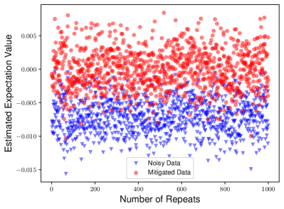
Figure 4: $1000$ noisy estimates $\eta^{(1)}$ (blue triangles) and error mitigated estimates $\eta$ (red dots) for the ideal expectation value $\operatorname{Tr}[O\rho]=0$. Here, the number of qubits is $8$.

Figure 5: Average expectation values for $1\leq n\leq 8$ qubits obtained with (red dots) and without (blue triangles) the error mitigation method. Each error bar is estimated by repeating the experiment $1000$ times.

V Conclusions

We have introduced a scalable method to mitigate measurement errors in computing expectation values of quantum observables, an essential building block of numerous quantum algorithms. The idea behind this method is to approximate the inverse of the noise matrix determined by the noisy measurement device using a small number of the Neumann series terms. Our method via the truncated Neumann series outperforms the exact matrix inversion method by significantly reducing the resource costs in time and samples of quantum states while only slightly degrading the error mitigation performance. In particular, our method works for any classical noise model and does not require the calibration procedure to learn the noise matrix a prior. Most importantly, the incurred error mitigation overhead is independent of the system size, as long as the noise resistance of the noisy measurement device is moderate. This property is beneficial and will be more and more important as the quantum circuit sizes increase. We have numerically tested this method and found that the computation accuracy is substantially improved. We believe that the proposed method will be useful for experimental measurement error mitigation in NISQ quantum devices.

Appendix A Proof of Eq. (6)

Proof.

By the definition of $\eta^{(1)}$, we have

$$\eta^{(1)}=\frac{1}{M}\sum_{m=1}^{M}O(\bm{s}^{m,1})=\frac{1}{M}\sum_{m=1}^{M}\sum_{\bm{x}\in\{0,1\}^{n}}O(\bm{x})\langle\bm{x}|\bm{s}^{m,1}\rangle=\sum_{\bm{x}\in\{0,1\}^{n}}O(\bm{x})\langle\bm{x}|\left(\frac{1}{M}\sum_{m=1}^{M}|\bm{s}^{m,1}\rangle\right).$$ (19)

The expectation value can be evaluated as

$$E^{(1)}\mathrel{\mathop{\mathchar 58\relax}}=\mathbb{E}[\eta^{(1)}] =\mathbb{E}\left[\sum_{\bm{x}\in\{0,1\}^{n}}O(\bm{x})\langle\bm{x}|\left(\frac{1}{M}\sum_{m=1}^{M}|\bm{s}^{m,1}\rangle\right)\right]$$ (20)

$$=\sum_{\bm{x}\in\{0,1\}^{n}}O(\bm{x})\langle\bm{x}|\mathbb{E}\left[\frac{1}{M}\sum_{m=1}^{M}|\bm{s}^{m,1}\rangle\right]$$ (21)

$$=\sum_{\bm{x}\in\{0,1\}^{n}}O(\bm{x})\langle\bm{x}|A\operatorname{vec}(\rho).$$ (22)

∎

Appendix B Proof of Theorem 1

Proof.

First of all, notice that

$$\left|\operatorname{Tr}[O\rho]-\sum_{k=1}^{K+1}c_{K}(k-1)E^{(k)}\right| =\left|\sum_{\bm{x}\in\{0,1\}^{n}}O(\bm{x})\langle\bm{x}|\operatorname{vec}(\rho)-\sum_{\bm{x}\in\{0,1\}^{n}}O(\bm{x})\langle\bm{x}|\left(\sum_{k=1}^{K+1}c_{K}(k-1)A^{k}\operatorname{vec}(\rho)\right)\right|$$ (23)

$$=\left|\sum_{\bm{x}\in\{0,1\}^{n}}O(\bm{x})\langle\bm{x}|\left(I-\sum_{k=1}^{K+1}c_{K}(k-1)A^{k}\right)\operatorname{vec}(\rho)\right|$$ (24)

$$=\left|\sum_{\bm{x}\in\{0,1\}^{n}}O(\bm{x})\langle\bm{x}|\left(I-A\left(\sum_{k=1}^{K+1}c_{K}(k-1)A^{k-1}\right)\right)\operatorname{vec}(\rho)\right|$$ (25)

$$=\left|\sum_{\bm{x}\in\{0,1\}^{n}}O(\bm{x})\langle\bm{x}|\left(I-A\left(\sum_{k=0}^{K}c_{K}(k)A^{k}\right)\right)\operatorname{vec}(\rho)\right|$$ (26)

$$=\left|\sum_{\bm{x}\in\{0,1\}^{n}}O(\bm{x})\langle\bm{x}|\left(I-A\left(\sum_{k=0}^{K}(I-A)^{k}\right)\right)\operatorname{vec}(\rho)\right|$$ (27)

$$=\left|\sum_{\bm{x}\in\{0,1\}^{n}}O(\bm{x})\langle\bm{x}|\left(I-\left(I-(I-A)^{K+1}\right)\right)\operatorname{vec}(\rho)\right|$$ (28)

$$=\left|\sum_{\bm{x}\in\{0,1\}^{n}}O(\bm{x})\langle\bm{x}|(I-A)^{K+1}\operatorname{vec}(\rho)\right|,$$ (29)

where (27) follows from (8) and (28) follows from the closed-form formula of a geometric series. Now we show that the quantity in (29) can be bounded from above. Define the induced matrix $1$-norm of a $m\times n$ matrix $B$ as

$$\left\lVert B\right\rVert_{1}\mathrel{\mathop{\mathchar 58\relax}}=\max_{1\leq j\leq n}\sum_{i=1}^{n}|B_{ij}|\equiv\max_{1\leq j\leq n}\sum_{i=1}^{n}|\left\langle{i}\right|B\left|{j}\right\rangle|,$$ (30)

which is simply the maximum absolute column sum of the matrix. Let $\rho(\bm{y})$ is the $\bm{y}$-th diagonal element of the quantum state $\rho$. Consider the following chain of inequalities:

$$\left|\sum_{\bm{x}\in\{0,1\}^{n}}O(\bm{x})\langle\bm{x}|(I-A)^{K+1}\operatorname{vec}(\rho)\right| =\left|\sum_{\bm{x}\in\{0,1\}^{n}}\sum_{\bm{y}\in\{0,1\}^{n}}O(\bm{x})\rho(\bm{y})\langle\bm{x}|(I-A)^{K+1}|\bm{y}\rangle\right|$$ (31a)

$$\leq\sum_{\bm{x}\in\{0,1\}^{n}}\sum_{\bm{y}\in\{0,1\}^{n}}|O(\bm{x})|\cdot\rho(\bm{y})\cdot\left|\langle\bm{x}|(I-A)^{K+1}|\bm{y}\rangle\right|$$ (31b)

$$\leq\sum_{\bm{x}\in\{0,1\}^{n}}\sum_{\bm{y}\in\{0,1\}^{n}}\rho(\bm{y})\left|\langle\bm{x}|(I-A)^{K+1}|\bm{y}\rangle\right|$$ (31c)

$$=\sum_{\bm{y}\in\{0,1\}^{n}}\rho(\bm{y})\sum_{\bm{x}\in\{0,1\}^{n}}\left|\langle\bm{x}|(I-A)^{K+1}|\bm{y}\rangle\right|$$ (31d)

$$\leq\sum_{\bm{y}\in\{0,1\}^{n}}\rho(\bm{y})\lVert(I-A)^{K+1}\lVert_{1}$$ (31e)

$$=\lVert(I-A)^{K+1}\lVert_{1}$$ (31f)

$$\leq\lVert I-A\lVert_{1}^{K+1}$$ (31g)

$$=\xi^{K+1},$$ (31h)

where (31c) follows from the assumption that $|O(\bm{x})|\leq 1$ (cf. Eq. (1)),  (31e) follows from the definition of induced matrix $1$-norm,  (31f) follows from the fact that $\rho$ is a quantum state and thus $\sum_{\bm{y}}\rho(\bm{y})=1$,  (31g) follows from the submultiplicativity property of the induced matrix norm, and (31h) follows from Lemma 3 stated below. We are done. ∎

Lemma 3.

Let $A$ be a column stochastic matrix of size $d\times d$. It holds that

$$\left\lVert I-A\right\rVert_{1}=\xi(A),$$ (32)

where $\xi(A)$ is defined in (7).

Proof.

Since $A$ is column stochastic, $I-A$ has non-negative diagonal elements and negative off-negative elements. Thus

$$\left\lVert I-A\right\rVert_{1} =\max_{1\leq j\leq d}\left(1-A_{jj}+\sum_{i\neq j}A_{ij}\right)$$ (33)

$$=\max_{1\leq j\leq d}\left(1-A_{jj}+1-A_{jj}\right)$$ (34)

$$=2\max_{1\leq j\leq d}\left(1-A_{jj}\right)$$ (35)

$$=2-2\min_{1\leq j\leq d}A_{jj}$$ (36)

$$=\mathrel{\mathop{\mathchar 58\relax}}\xi(A),$$ (37)

where the second line follows from the fact that $A$ is column stochastic. ∎

Appendix C Sequential measurements

In the Appendix, we prove that the classical noise model describing the sequential measurement repeating $k$ times is effectively characterized by the stochastic matrix $A^{k}$. We begin with the simple case $k=2$. Since the noise model is classical and linear in the input, it suffices to consider the computational basis states as inputs. As shown in Fig. 6, we apply the noisy quantum measurement device two times sequentially on the input state $|{\bm{x}}\rangle\!\langle{\bm{x}}|$ in computational basis where $\bm{x}\in\{0,1\}^{n}$. Assume the measurement outcome of the first measurement is $\bm{y}$ and the measurement outcome of the second measurement is $\bm{z}$, where $\bm{y},\bm{z}\in\{0,1\}^{n}$. Assume that the noise matrix associated with this sequential measurement is $A^{\prime}$. That is, the probability of obtaining the outcome $\bm{z}$ provided the true outcome is $\bm{x}$ is given by $A^{\prime}_{\bm{z}\bm{x}}$. Practically, we input $|{\bm{x}}\rangle\!\langle{\bm{x}}|$ to the first noisy measurement device and obtain the outcome $\bm{y}$. The probability of this event is $A_{\bm{y}\bm{x}}$, by the definition of the noise matrix. Similarly, we input $|{\bm{y}}\rangle\!\langle{\bm{y}}|$ to the second noisy measurement device and obtain the outcome $\bm{z}$. The probability of this event is $A_{\bm{z}\bm{y}}$. Inspecting the chain $\bm{x}\to\bm{y}\to\bm{z}$, we have

$$A^{\prime}_{\bm{z}\bm{x}}=\sum_{\bm{y}\in\{0,1\}^{n}}A_{\bm{y}\bm{x}}A_{\bm{z}\bm{y}}=A^{2}_{\bm{z}\bm{x}}.$$ (38)

The above analysis justifies that the classical noise model describing the sequential measurement repeating $2$ times is effectively characterized by the stochastic matrix $A^{2}$. The general case can be analyzed similarly.

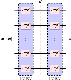
Figure 6: Apply the noisy quantum measurement device two times sequentially on the input state $|{\bm{x}}\rangle\!\langle{\bm{x}}|$ where $\bm{x}\in\{0,1\}^{n}$. The measurement outcome of the first measurement is $\bm{y}$ and the measurement outcome of the second measurement is $\bm{z}$.

Mathematically, quantum measurements can be modeled as quantum-classical quantum channels (Wilde, 2016, Chapter 4.6.6) where they take a quantum system to a classical one. Experimentally, the implementation of quantum measurement is platform-dependent and has different characterizations. For example, the fabrication and control of quantum coherent superconducting circuits have enabled experiments that implement quantum measurement Naghiloo (2019). Based on the outcome data, experimental measurements are typically categorized into two types: those only output classical outcomes and those output both classical outcomes and quantum states. That is, besides the usually classical outcome sequences, the measurement device will also output a quantum state on the computational basis corresponding to the classical outcome. For the former type, we can implement the sequential measurement via the qubit reset Egger et al. (2018); Magnard et al. (2018); Yirka and Subasi (2020) approach, by which we mean the ability to re-initialize the qubits into a known state, usually a state in the computational basis, during the course of the computation. Technically, when the $i$-th noisy measurement outputs an outcome sequence $\bm{s}^{i}\in\{0,1\}^{n}$, we use the qubit reset technique to prepare the computational basis state $|\bm{s}^{i}\rangle\!\langle\bm{s}^{i}|$ and feed it to the $(i+1)$-th noisy measurement (cf. Fig. 6). In this case, the noisy measurement device can be reused. For the latter type, the sequential measurement can be implemented efficiently: when the $i$-th noisy measurement outputs a classical sequence and a quantum state on the computational basis, we feed the quantum state to the $(i+1)$-th noisy measurement.

Appendix D Proof of Proposition 2

Proof.

By definition,

$$\eta=\sum_{k=1}^{K+1}c_{K}(k-1)\eta^{(k)}=\frac{1}{M}\sum_{k=1}^{K+1}\sum_{m=1}^{M}c_{K}(k-1)O(\bm{s}^{m,k})=\frac{1}{M(K+1)}\sum_{k=1}^{K+1}\sum_{m=1}^{M}(K+1)c_{K}(k-1)O(\bm{s}^{m,k}).$$ (39)

Introducing the new random variables $X_{m,k}\mathrel{\mathop{\mathchar 58\relax}}=(K+1)c_{K}(k-1)O(\bm{s}^{m,k})$, we have

$$\eta=\frac{1}{M(K+1)}\sum_{k=1}^{K+1}\sum_{m=1}^{M}X_{m,k}.$$ (40)

Intuitively, Eq. (40) says that $\eta$ can be viewed as the empirical mean value of the set of random variables

$$\left\{X_{m,k}\mathrel{\mathop{\mathchar 58\relax}}m=1,\cdots,M;k=1,\cdots,K+1\right\}.$$ (41)

First, we show that the absolute value of each $X_{m,k}$ is upper bounded as

$$|X_{m,k}|=|(K+1)c_{K}(k-1)O(\bm{s}^{m,k})|\leq(K+1)|c_{K}(k-1)||O(\bm{s}^{m,k})|\leq(K+1)|c_{K}(k-1)|,$$ (42)

where the second inequality follows from the assumption of $O$ (cf. Eq. (1)). Then, we show that $\eta$ is an unbiased estimator of the quantity $\sum_{k=1}^{K+1}c_{K}(k-1)E^{(k)}$:

$$\mathbb{E}[\eta] =\mathbb{E}\left[\frac{1}{M(K+1)}\sum_{k=1}^{K+1}\sum_{m=1}^{M}X_{m,k}\right]$$ (43a)

$$=\mathbb{E}\left[\frac{1}{M}\sum_{k=1}^{K+1}\sum_{m=1}^{M}c_{K}(k-1)O(\bm{s}^{m,k})\right]$$ (43b)

$$=\sum_{k=1}^{K+1}c_{K}(k-1)\left(\sum_{\bm{x}}O(\bm{x})\langle\bm{x}|\mathbb{E}_{M}\left[\frac{1}{M}\sum_{m=1}^{M}|\bm{s}^{m,k}\rangle\right]\right)$$ (43c)

$$=\sum_{k=1}^{K+1}c_{K}(k-1)\left(\sum_{\bm{x}}O(\bm{x})\langle\bm{x}|A^{k}\operatorname{vec}(\rho)\right)$$ (43d)

$$=\sum_{k=1}^{K+1}c_{K}(k-1)E^{(k)},$$ (43e)

where the last equality follows from (11). Eqs. (42) and (43) together guarantee that the prerequisites of the Hoeffding’s inequality hold. By the Hoeffding’s equality, we have

$$\Pr\left\{\left|\eta-\sum_{k=1}^{K+1}c_{K}(k-1)E^{(k)}\right|\geq\varepsilon\right\} \leq 2\exp\left(-\frac{2M^{2}(K+1)^{2}\varepsilon^{2}}{4\sum_{k=1}^{K+1}\sum_{m=1}^{M}((K+1)c_{K}(k))^{2}}\right)$$ (44)

$$=2\exp\left(-\frac{2M^{2}(K+1)^{2}\varepsilon^{2}}{4M(K+1)^{3}\left(\sum_{k=0}^{K}[c_{K}(k)]^{2}\right)}\right)$$ (45)

$$=2\exp\left(-\frac{M\varepsilon^{2}}{2(K+1)\Delta}\right),$$ (46)

where $\Delta\mathrel{\mathop{\mathchar 58\relax}}=\sum_{k=1}^{K+1}[c_{K}(k)]^{2}=\binom{2K+2}{K+1}-1$. Solving

$$2\exp\left(-\frac{M\varepsilon^{2}}{2(K+1)\Delta}\right)\leq\delta$$ (47)

gives

$$M\geq 2(K+1)\Delta\log(2/\delta)/\varepsilon^{2}.$$ (48)

To summarize, choosing $K=\left\lceil\log\varepsilon/\log\xi-1\right\rceil$ and $M=\lceil 2(K+1)\Delta\log(2/\delta)/\varepsilon^{2}\rceil$, we are able obtain the following two statements

$$\Pr\left\{\left|\eta-\sum_{k=1}^{K+1}c_{K}(k-1)E^{(k)}\right|\geq\varepsilon\right\}\leq\delta,$$ (49)

$$\left|\operatorname{Tr}[O\rho]-\sum_{k=1}^{K+1}c_{K}(k-1)E^{(k)}\right|\leq\varepsilon,$$ (50)

where the first one is shown above and the second one is proved in Theorem 1. Using the union bound and the triangle inequality, we conclude that $\eta$ can estimate the ideal expectation value $\operatorname{Tr}[O\rho]$ with error $2\varepsilon$ at a probability greater than $1-\delta$. ∎

References

- McArdle et al. (2020) S. McArdle, S. Endo, A. Aspuru-Guzik, S. C. Benjamin, and X. Yuan, Reviews of Modern Physics 92, 015003 (2020).
- Cerezo et al. (2020) M. Cerezo, A. Arrasmith, R. Babbush, S. C. Benjamin, S. Endo, K. Fujii, J. R. McClean, K. Mitarai, X. Yuan, L. Cincio, et al., arXiv preprint arXiv:2012.09265 (2020).
- Bharti et al. (2021) K. Bharti, A. Cervera-Lierta, T. H. Kyaw, T. Haug, S. Alperin-Lea, A. Anand, M. Degroote, H. Heimonen, J. S. Kottmann, T. Menke, et al., arXiv preprint arXiv:2101.08448 (2021).
- Endo et al. (2021) S. Endo, Z. Cai, S. C. Benjamin, and X. Yuan, Journal of the Physical Society of Japan 90, 032001 (2021).
- Preskill (2018) J. Preskill, Quantum 2, 79 (2018).
- Temme et al. (2017) K. Temme, S. Bravyi, and J. M. Gambetta, Physical Review Letters 119, 180509 (2017).
- Endo et al. (2018) S. Endo, S. C. Benjamin, and Y. Li, Physical Review X 8, 031027 (2018).
- Li and Benjamin (2017) Y. Li and S. C. Benjamin, Physical Review X 7, 021050 (2017).
- McClean et al. (2017) J. R. McClean, M. E. Kimchi-Schwartz, J. Carter, and W. A. De Jong, Physical Review A 95, 042308 (2017).
- McClean et al. (2020) J. R. McClean, Z. Jiang, N. Rubin, R. Babbush, and H. Neven, Nature Communications 11, 636 (2020).
- McArdle et al. (2019) S. McArdle, X. Yuan, and S. Benjamin, Physical Review Letters 122, 180501 (2019).
- Bonet-Monroig et al. (2018) X. Bonet-Monroig, R. Sagastizabal, M. Singh, and T. O’Brien, Physical Review A 98, 062339 (2018).
- He et al. (2020) A. He, B. Nachman, W. A. de Jong, and C. W. Bauer, Physical Review A 102, 012426 (2020).
- Giurgica-Tiron et al. (2020) T. Giurgica-Tiron, Y. Hindy, R. LaRose, A. Mari, and W. J. Zeng, arXiv preprint arXiv:2005.10921 (2020).
- Kandala et al. (2019) A. Kandala, K. Temme, A. D. Córcoles, A. Mezzacapo, J. M. Chow, and J. M. Gambetta, Nature 567, 491 (2019).
- Sun et al. (2021) J. Sun, X. Yuan, T. Tsunoda, V. Vedral, S. C. Benjamin, and S. Endo, Physical Review Applied 15, 034026 (2021).
- Czarnik et al. (2020) P. Czarnik, A. Arrasmith, P. J. Coles, and L. Cincio, arXiv preprint arXiv:2005.10189 (2020).
- Chow et al. (2012) J. M. Chow, J. M. Gambetta, A. D. Corcoles, S. T. Merkel, J. A. Smolin, C. Rigetti, S. Poletto, G. A. Keefe, M. B. Rothwell, J. R. Rozen, et al., Physical Review Letters 109, 060501 (2012).
- Chen et al. (2019) Y. Chen, M. Farahzad, S. Yoo, and T.-C. Wei, Physical Review A 100, 052315 (2019).
- Geller (2020) M. R. Geller, Quantum Science and Technology 5, 03LT01 (2020).
- Maciejewski et al. (2020) F. B. Maciejewski, Z. Zimborás, and M. Oszmaniec, Quantum 4, 257 (2020).
- Tannu and Qureshi (2019) S. S. Tannu and M. K. Qureshi, in Proceedings of the 52nd Annual IEEE/ACM International Symposium on Microarchitecture (2019) pp. 279–290.
- Nachman et al. (2019) B. Nachman, M. Urbanek, W. A. de Jong, and C. W. Bauer, arXiv preprint arXiv:1910.01969 (2019).
- Hicks et al. (2021) R. Hicks, C. W. Bauer, and B. Nachman, Physical Review A 103, 022407 (2021).
- Bravyi et al. (2020) S. Bravyi, S. Sheldon, A. Kandala, D. C. Mckay, and J. M. Gambetta, arXiv preprint arXiv:2006.14044 (2020).
- Geller and Sun (2020) M. R. Geller and M. Sun, arXiv preprint arXiv:2001.09980 (2020).
- Murali et al. (2020) P. Murali, D. C. McKay, M. Martonosi, and A. Javadi-Abhari, in Proceedings of the Twenty-Fifth International Conference on Architectural Support for Programming Languages and Operating Systems (2020) pp. 1001–1016.
- Kwon and Bae (2020) H. Kwon and J. Bae, IEEE Transactions on Computers (2020).
- Funcke et al. (2020) L. Funcke, T. Hartung, K. Jansen, S. Kühn, P. Stornati, and X. Wang, arXiv preprint arXiv:2007.03663 (2020).
- Zheng et al. (2020) M. Zheng, A. Li, T. Terlaky, and X. Yang, arXiv preprint arXiv:2010.09188 (2020).
- Maciejewski et al. (2021) F. B. Maciejewski, F. Baccari, Z. Zimborás, and M. Oszmaniec, arXiv preprint arXiv:2101.02331 (2021).
- Barron and Wood (2020) G. S. Barron and C. J. Wood, arXiv preprint arXiv:2010.08520 (2020).
- Pashayan et al. (2015) H. Pashayan, J. J. Wallman, and S. D. Bartlett, Physical Review Letters 115, 070501 (2015).
- Howard and Campbell (2017) M. Howard and E. Campbell, Physical Review Letters 118, 090501 (2017).
- Takagi (2020) R. Takagi, arXiv preprint arXiv:2006.12509 (2020).
- Jiang et al. (2020) J. Jiang, K. Wang, and X. Wang, arXiv preprint arXiv:2012.10959 (2020).
- Regula et al. (2021) B. Regula, R. Takagi, and M. Gu, arXiv preprint arXiv:2102.07773 (2021).
- Berg et al. (2020) E. v. d. Berg, Z. K. Minev, and K. Temme, arXiv preprint arXiv:2012.09738 (2020).
- Peruzzo et al. (2014) A. Peruzzo, J. McClean, P. Shadbolt, M.-H. Yung, X.-Q. Zhou, P. J. Love, A. Aspuru-Guzik, and J. L. O’brien, Nature Communications 5, 4213 (2014).
- McClean et al. (2016) J. R. McClean, J. Romero, R. Babbush, and A. Aspuru-Guzik, New Journal of Physics 18, 023023 (2016).
- Farhi et al. (2014) E. Farhi, J. Goldstone, and S. Gutmann, arXiv preprint arXiv:1411.4028 (2014).
- Biamonte et al. (2017) J. Biamonte, P. Wittek, N. Pancotti, P. Rebentrost, N. Wiebe, and S. Lloyd, Nature 549, 195 (2017).
- Havlíček et al. (2019) V. Havlíček, A. D. Córcoles, K. Temme, A. W. Harrow, A. Kandala, J. M. Chow, and J. M. Gambetta, Nature 567, 209 (2019).
- Hoeffding (1963) W. Hoeffding, Journal of the American Statistical Association 58, 13 (1963).
- (45) The quantum circuit diagrams in this work are created using the quantikz package Kay (2018).
- Wu et al. (2013) M. Wu, B. Yin, A. Vosoughi, C. Studer, J. R. Cavallaro, and C. Dick, in 2013 IEEE International Symposium on Circuits and Systems (ISCAS) (IEEE, 2013) pp. 2155–2158.
- Stewart (1998) G. W. Stewart, Matrix Algorithms: Volume 1: Basic Decompositions (SIAM, 1998).
- Kay (2018) A. Kay, arXiv preprint arXiv:1809.03842 (2018), 10.17637/rh.7000520.v4.
- Wilde (2016) M. M. Wilde, Quantum Information Theory 2nd Edition (Cambridge University Press, 2016).
- Naghiloo (2019) M. Naghiloo, arXiv preprint arXiv:1904.09291 (2019).
- Egger et al. (2018) D. J. Egger, M. Werninghaus, M. Ganzhorn, G. Salis, A. Fuhrer, P. Mueller, and S. Filipp, Physical Review Applied 10, 044030 (2018).
- Magnard et al. (2018) P. Magnard, P. Kurpiers, B. Royer, T. Walter, J.-C. Besse, S. Gasparinetti, M. Pechal, J. Heinsoo, S. Storz, A. Blais, et al., Physical Review Letters 121, 060502 (2018).
- Yirka and Subasi (2020) J. Yirka and Y. Subasi, arXiv preprint arXiv:2010.03080 (2020).