FedCor: Correlation-Based Active Client Selection Strategy for Heterogeneous Federated Learning

Minxue Tang1, Xuefei Ning2, Yitu Wang1, Jingwei Sun1, Yu Wang2, Hai Li1, Yiran Chen1
1Department of Electrical and Computer Engineering, Duke University
2Department of Electronic Engineering, Tsinghua University
1{minxue.tang,yitu.wang,jingwei.sun,hai.li,yiran.chen}@duke.edu
2foxdoraame@gmail.com  2yu-wang@tsinghua.edu.cn
Corresponding Author
Abstract

Client-wise data heterogeneity is one of the major issues that hinder effective training in federated learning (FL). Since the data distribution on each client may vary dramatically, the client selection strategy can significantly influence the convergence rate of the FL process. Active client selection strategies are popularly proposed in recent studies. However, they neglect the loss correlations between the clients and achieve only marginal improvement compared to the uniform selection strategy. In this work, we propose FedCor—an FL framework built on a correlation-based client selection strategy, to boost the convergence rate of FL. Specifically, we first model the loss correlations between the clients with a Gaussian Process (GP). Based on the GP model, we derive a client selection strategy with a significant reduction of expected global loss in each round. Besides, we develop an efficient GP training method with a low communication overhead in the FL scenario by utilizing the covariance stationarity. Our experimental results show that compared to the state-of-the-art method, FedCorr can improve the convergence rates by 34%99%similar-topercent34percent9934\%\sim 99\% and 26%51%similar-topercent26percent5126\%\sim 51\% on FMNIST and CIFAR-10, respectively.

1 Introduction

As a newly emerging distributed learning paradigm, federated learning (FL) [12, 13, 23, 9, 17] has recently attracted attention because of the offered data privacy. FL aims at dealing with scenarios where training data is distributed across a number of clients. Considering limited communication bandwidth and the privacy requirement, in each communication round, FL usually selects only a fraction of clients, and the selected clients will perform multiple iterations of local updating without exposing their own datasets [23]. This special scenario also introduces other challenges that distinguish FL from the conventional distributed learning [2, 35].

One major challenge in FL is the high degree of client-wise data heterogeneity [17], which is the inherent characteristic of a large number of clients. There have been many studies [27, 18, 20, 10, 32, 25, 16, 15] trying to tackle non-IID (independent and identically distributed) and unbalanced data of the clients in FL. Most of these studies [18, 20, 10, 32] focus on amending the local model updates or the central aggregation based on FedAvg [23].

Recently, active client selection arises as a complement of the aforementioned studies, aiming at accelerating the convergence of FL with non-IID data. Some recent studies propose to assign higher probability of being selected to the clients with larger training loss value [6, 4]. However, they neglect the correlations between the clients and consider their losses independently, which leads to only marginal performance improvement. In this paper, we propose a correlation-based active client selection strategy that can effectively alleviate the accuracy degradation caused by data heterogeneity and significantly boost the convergence of FL. Our key idea is mainly based on the following intuitions:

  1. 1.

    Clients do not contribute equivalently. For example, training with a large and balanced dataset on a “good” client can reduce the losses of most clients, while training with a small and extremely biased dataset on a “bad” client may increase the losses of other clients.

  2. 2.

    Clients do not contribute independently. The influence of selecting one client depends on the other selected clients because their local updates will be aggregated.
Refer to caption
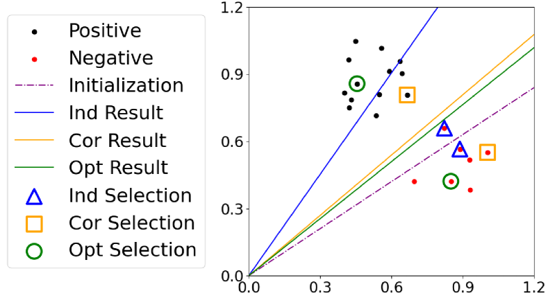
Figure 1: A toy experiment of different client selection strategies.

A toy experiment shown in Fig. 1 also illustrates the necessity of considering the correlations for client selection. In this experiment, each client has only one data sample, and thus each data point in the figure represents a client. The task is to select two clients (different markers represent the client selections of different strategies) for training a binary classifier (shown as the lines). The selection strategy that independently selects two clients with the highest local losses (“Ind Result”) fails to reduce the global loss. In contrast, our method considers the correlations between the clients (“Cor Result”) and derives a client selection that can achieve an almost lowest global loss (“Opt Result”).

Based on the above intuitions, this work proposes FedCor, an FL framework built on a correlation-based client selection strategy, to boost the convergence of FL. Our main contributions are summarized as follows:

  1. 1.

    We model the client loss changes with a Gaussian Process (GP) and propose an interpretable client selection strategy with a significant reduction of the expected global loss in each communication round.

  2. 2.

    We propose a GP training method that utilizes the covariance stationarity to reduce the communication cost. Experiments show that the GP trained with our method can capture the client correlations well.

  3. 3.

    Experimental results demonstrate that FedCor stabilizes the training convergence and significantly improves the convergence rates by 34%99%similar-topercent34percent9934\%\sim 99\% and 26%51%similar-topercent26percent5126\%\sim 51\% on FMNIST and CIFAR-10, respectively.

2 Related Work

An important characteristic of FL [12, 13, 23] is the heterogeneity of clients, which raises new challenges of the training [9, 17, 31]. There are two kinds of heterogeneity in FL: systemic heterogeneity (computation ability, communication bandwidth, etc.) and statistical heterogeneity (non-IID, imbalanced data distribution) [18, 17]. This work mainly focuses on the latter one. A number of methods have been proposed to improve the basic FL algorithm, FedAvg [23], in heterogeneous settings. Some of them manipulate the local training loss like adding regularization terms to stabilized the training [18, 26, 20, 10, 8], while some other works amend the aggregation method to reduce the variance [32, 24].

Complementary to such methods, another way to improve the convergence of FL in non-IID settings is active client selection, which tries to strategically select clients for training in each round in stead of uniformly selecting. Goetz et al. [6] first propose to assign a high selection probability to the clients with large local loss. Cho et al. [4] select C𝐶C clients with the largest loss among a randomly sampled subset 𝔸𝕌𝔸𝕌{\mathbb{A}}\subseteq{\mathbb{U}} with size d>C𝑑𝐶d>C to reduce the selection bias. However, neither of them consider the correlations between clients while making the client selection.

3 Preliminary

FL seeks for a global model 𝒘𝒘{\bm{w}} that achieves the best performance (e.g., the highest classification accuracy) on all N𝑁N clients. The global loss function in FL is defined as:

L(𝒘)𝐿𝒘\displaystyle L({\bm{w}}) =k=1N|𝔻k|j|𝔻j|l(𝒘;𝔻k)=k=1Npklk(𝒘),absentsuperscriptsubscript𝑘1𝑁subscript𝔻𝑘subscript𝑗subscript𝔻𝑗𝑙𝒘subscript𝔻𝑘superscriptsubscript𝑘1𝑁subscript𝑝𝑘subscript𝑙𝑘𝒘\displaystyle=\sum_{k=1}^{N}\frac{|{\mathbb{D}}_{k}|}{\sum_{j}|{\mathbb{D}}_{j}|}l({\bm{w}};{\mathbb{D}}_{k})=\sum_{k=1}^{N}p_{k}l_{k}({\bm{w}}), (1)
lk(𝒘)subscript𝑙𝑘𝒘\displaystyle l_{k}({\bm{w}}) =l(𝒘;𝔻k)=1|𝔻k|ξ𝔻kl(𝒘;ξ),absent𝑙𝒘subscript𝔻𝑘1subscript𝔻𝑘subscript𝜉subscript𝔻𝑘𝑙𝒘𝜉\displaystyle=l({\bm{w}};{\mathbb{D}}_{k})=\frac{1}{|{\mathbb{D}}_{k}|}\sum_{\mathbf{\xi}\in{\mathbb{D}}_{k}}l({\bm{w}};\mathbf{\xi}), (2)

where l(𝒘;ξ)𝑙𝒘𝜉l({\bm{w}};\mathbf{\xi}) is the objective loss of data sample ξ𝜉\mathbf{\xi} evaluated on model 𝒘𝒘{\bm{w}}. We refer to lk(𝒘)subscript𝑙𝑘𝒘l_{k}({\bm{w}}) as the local loss of client k𝑘k, which is evaluated with the local dataset 𝔻ksubscript𝔻𝑘{\mathbb{D}}_{k} (of size |𝔻k|subscript𝔻𝑘|{\mathbb{D}}_{k}|) on client k𝑘k. The weight pk=|𝔻k|/j|𝔻j|subscript𝑝𝑘subscript𝔻𝑘subscript𝑗subscript𝔻𝑗p_{k}=|{\mathbb{D}}_{k}|/\sum_{j}|{\mathbb{D}}_{j}| of the client k𝑘k is proportional to the size of its local dataset.

In consideration of the privacy and communication constraints, FL algorithms usually assume partial client participation and perform local model updates. In particular, in communication round t𝑡t, only a subset 𝕂tsubscript𝕂𝑡{\mathbb{K}}_{t} with size |𝕂t|=CNsubscript𝕂𝑡𝐶𝑁|{\mathbb{K}}_{t}|=C\leq N of the overall client set 𝕌𝕌{\mathbb{U}} is selected to receive the global model 𝒘tsuperscript𝒘𝑡{\bm{w}}^{t} and conduct training with their local dataset for several iterations independently. After the local training, the server collects the trained models from these selected clients and aggregates them (usually by averaging [23]) to produce a new global model 𝒘t+1superscript𝒘𝑡1{\bm{w}}^{t+1}. We formulate this procedure as follows:

𝒘kt+1superscriptsubscript𝒘𝑘𝑡1\displaystyle{\bm{w}}_{k}^{t+1} =𝒘tηt~lk(𝒘t),absentsuperscript𝒘𝑡subscript𝜂𝑡~subscript𝑙𝑘superscript𝒘𝑡\displaystyle={\bm{w}}^{t}-\eta_{t}\tilde{\nabla}l_{k}({\bm{w}}^{t}), (3)
𝒘t+1(𝕂t)superscript𝒘𝑡1subscript𝕂𝑡\displaystyle{\bm{w}}^{t+1}({\mathbb{K}}_{t}) =1Ck𝕂t𝒘kt+1absent1𝐶subscript𝑘subscript𝕂𝑡superscriptsubscript𝒘𝑘𝑡1\displaystyle=\frac{1}{C}\sum_{k\in{\mathbb{K}}_{t}}{\bm{w}}_{k}^{t+1} (4)
=𝒘tηtCk𝕂t~lk(𝒘t),absentsuperscript𝒘𝑡subscript𝜂𝑡𝐶subscript𝑘subscript𝕂𝑡~subscript𝑙𝑘superscript𝒘𝑡\displaystyle={\bm{w}}^{t}-\frac{\eta_{t}}{C}\sum_{k\in{\mathbb{K}}_{t}}\tilde{\nabla}l_{k}({\bm{w}}^{t}), (5)

where ηtsubscript𝜂𝑡\eta_{t} is the learning rate and ~lk(𝒘t)~subscript𝑙𝑘superscript𝒘𝑡\tilde{\nabla}l_{k}({\bm{w}}^{t}) is the equivalent cumulative gradient [32] in the t𝑡t-th communication round. More specifically, for an arbitrary optimizer on the client k𝑘k, it produces Δ𝒘kt,τ=η𝒅kt,τΔsuperscriptsubscript𝒘𝑘𝑡𝜏𝜂subscriptsuperscript𝒅𝑡𝜏𝑘\Delta{\bm{w}}_{k}^{t,\tau}=-\eta\bm{d}^{t,\tau}_{k} as the local model update at the τ𝜏\tau-th iteration in this round, and the cumulative gradient is calculated as ~lk(𝒘t)=τ𝒅kt,τ~subscript𝑙𝑘superscript𝒘𝑡subscript𝜏superscriptsubscript𝒅𝑘𝑡𝜏\tilde{\nabla}l_{k}({\bm{w}}^{t})=\sum_{\tau}\bm{d}_{k}^{t,\tau}.

4 Methodology

In this section, we elaborate our proposed method, i.e., FedCor, that can effectively boost the convergence of FL. We first formulate our goal of accelerating the convergence of FL as optimization problems that maximize the posterior expectation of loss decrease in Sec. 4.1. Then, Sec. 4.2 demonstrates empirical evidence that the prior distribution of loss changes in each communication round can be modeled as Gaussian Processes (GP). Based on this observation, we utilize GP to solve the optimization problems and obtain an effective client selection strategy for heterogeneous FL in Sec. 4.3. We further analyze the selection criterion of our client selection strategy and give out its intuitive interpretation in Sec. 4.4. Finally, in Sec. 4.5, we describe how we train the GP parameters in communication-constrained FL.

4.1 Problem Formulation

To achieve a fast convergence, we hope to find the client selection strategy which can lead to the maximal global loss decrease after each communication round. Accordingly, we define our target as solving a series of optimization problems, one for each communication round t𝑡t:

min𝕂tsubscriptsubscript𝕂𝑡\displaystyle\min_{{\mathbb{K}}_{t}} ΔLt(𝕂t)=L(𝒘t+1(𝕂t))L(𝒘t)Δsuperscript𝐿𝑡subscript𝕂𝑡𝐿superscript𝒘𝑡1subscript𝕂𝑡𝐿superscript𝒘𝑡\displaystyle\Delta L^{t}({\mathbb{K}}_{t})=L({\bm{w}}^{t+1}({\mathbb{K}}_{t}))-L({\bm{w}}^{t}) (6)
subject to 𝒘t+1(𝕂t)=𝒘tηtCk𝕂t~lk(𝒘t).superscript𝒘𝑡1subscript𝕂𝑡superscript𝒘𝑡subscript𝜂𝑡𝐶subscript𝑘subscript𝕂𝑡~subscript𝑙𝑘superscript𝒘𝑡\displaystyle{\bm{w}}^{t+1}({\mathbb{K}}_{t})={\bm{w}}^{t}-\frac{\eta_{t}}{C}\sum_{k\in{\mathbb{K}}_{t}}\tilde{\nabla}l_{k}({\bm{w}}^{t}).

It is impractical in FL to search for the best client selection with multiple trials of different client selections since it introduces large communication and computation overhead. Therefore, we need an efficient way to predict the global loss decreases for different client selections and make a decision with very limited trials. To achieve this goal, we first reformulate the optimization problem in Eq. 6 with the following lemma. The proof of this lemma is in Sec. A.2.

Lemma 1.

The optimization problem in Eq. 6 is approximately equivalent to the following probabilistic form.

min𝕂t𝔼Δ𝐥t|Δ𝒍𝕂tt(𝕂t)[ipiΔlit]=ipiμ~it(Δ𝒍𝕂tt(𝕂t)),subscriptsubscript𝕂𝑡subscript𝔼conditionalΔsuperscript𝐥𝑡Δsubscriptsuperscript𝒍𝑡subscript𝕂𝑡subscript𝕂𝑡delimited-[]subscript𝑖subscript𝑝𝑖Δsubscriptsuperscript𝑙𝑡𝑖subscript𝑖subscript𝑝𝑖subscriptsuperscript~𝜇𝑡𝑖Δsubscriptsuperscript𝒍𝑡subscript𝕂𝑡subscript𝕂𝑡\min_{{\mathbb{K}}_{t}}\quad\mathbb{E}_{\Delta{\mathbf{l}}^{t}|\Delta\bm{l}^{t}_{{\mathbb{K}}_{t}}({\mathbb{K}}_{t})}\Big{[}\sum_{i}p_{i}\Delta l^{t}_{i}\Big{]}=\sum_{i}p_{i}\tilde{\mu}^{t}_{i}(\Delta\bm{l}^{t}_{{\mathbb{K}}_{t}}({\mathbb{K}}_{t})), (7)

where Δ𝐥t=[Δl1t,,ΔlNt]Δsuperscript𝐥𝑡Δsubscriptsuperscriptl𝑡1Δsubscriptsuperscriptl𝑡𝑁\Delta{\mathbf{l}}^{t}=[\Delta{\textnormal{l}}^{t}_{1},\cdots,\Delta{\textnormal{l}}^{t}_{N}] is the loss changes of all clients in round t𝑡t, which is a random variable w.r.t random client selection in round t𝑡t. 𝛍~t(Δ𝐥𝕂tt(𝕂t))superscript~𝛍𝑡Δsubscriptsuperscript𝐥𝑡subscript𝕂𝑡subscript𝕂𝑡\tilde{\bm{\mu}}^{t}(\Delta\bm{l}^{t}_{{\mathbb{K}}_{t}}({\mathbb{K}}_{t})) is the posterior mean of Δ𝐥tΔsuperscript𝐥𝑡\Delta{\mathbf{l}}^{t} conditioned on Δ𝐥𝕂tt(𝕂t)=[Δlit(𝕂t)]i𝕂tΔsubscriptsuperscript𝐥𝑡subscript𝕂𝑡subscript𝕂𝑡subscriptdelimited-[]Δsubscriptsuperscript𝑙𝑡𝑖subscript𝕂𝑡𝑖subscript𝕂𝑡\Delta\bm{l}^{t}_{{\mathbb{K}}_{t}}({\mathbb{K}}_{t})=[\Delta l^{t}_{i}({\mathbb{K}}_{t})]_{i\in{\mathbb{K}}_{t}}.

The reformulated objective in Eq. 7 tells that if we can predict the loss changes of those clients selected for training (Δ𝒍𝕂tt(𝕂t)Δsubscriptsuperscript𝒍𝑡subscript𝕂𝑡subscript𝕂𝑡\Delta\bm{l}^{t}_{{\mathbb{K}}_{t}}({\mathbb{K}}_{t})), we can predict the global loss change with its posterior mean and make decision according to it. Now what we need is a probabilistic model of the loss changes Δ𝐥tΔsuperscript𝐥𝑡\Delta{\mathbf{l}}^{t} to make the prediction and calculate the posterior.

4.2 Modeling Loss Changes with GP

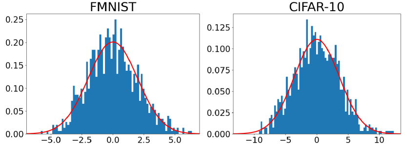
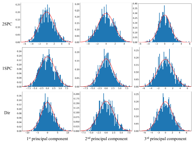
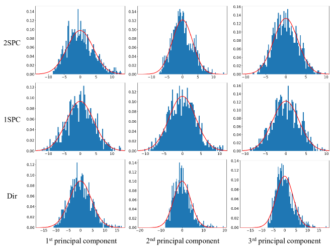
It is a common practice to assume a GP prior over an unknown objective function in Bayesian Optimization [3, 30]. Our preliminary investigation (partly) shown in Fig. 2 also indicates that the prior distribution of the loss changes in one communication round follow a GP. Specifically, we randomly sample a number of client selections and perform one round of training to get samples of the loss changes. Then, we conduct PCA on these loss change samples and plot histograms of the first several principle components. The red line in the Fig. 2 is the Gaussian PDF with the sample mean and sample variance. And we can see that this Gaussian distribution can approximate the distribution of the samples well. A mathematical explanation of this observation is also given out in Sec. A.1.

Accordingly, we propose to model the loss changes in one communication round t𝑡t with a GP prior as follows:

Δ𝐥t=[Δl1t,,ΔlNt]𝒩(Δ𝒍t;𝝁t,𝚺t).Δsuperscript𝐥𝑡Δsubscriptsuperscriptl𝑡1Δsubscriptsuperscriptl𝑡𝑁similar-to𝒩Δsuperscript𝒍𝑡superscript𝝁𝑡superscript𝚺𝑡\Delta{\mathbf{l}}^{t}=[\Delta{\textnormal{l}}^{t}_{1},\cdots,\Delta{\textnormal{l}}^{t}_{N}]\sim\mathcal{N}(\Delta\bm{l}^{t};\bm{\mu}^{t},\bm{\Sigma}^{t}). (8)

Remark. In order to efficiently learn the covariance in FL, rather than directly working with the covariance matrix, we embed all clients into a continuous vector space and use a kernel function to calculate the covariance (see Sec. 4.5). Thus, we still use the term GP instead of Multivariate Gaussian Distribution, though the dimension of Δ𝐥tΔsuperscript𝐥𝑡\Delta{\mathbf{l}}^{t} is finite.

A good property of GP is that we can get a closed form of the posterior expectation in Eq. 7, which makes our client selection strategy interpretable. In the next sections, we will propose our client selection strategy based on the GP model, and then give an interpretation of it. We leave the training method for the parameters (𝝁t,𝚺tsuperscript𝝁𝑡superscript𝚺𝑡\bm{\mu}^{t},\bm{\Sigma}^{t}) in GP to Sec. 4.5.

Refer to caption
Figure 2: Histograms of the first principle component in Non-IID FL [23]. More details and full results can be found in Sec. D.2.

4.3 Client Selection Strategy

While we have get the probabilistic model to calculate the posterior expectation, it is still not determined how to predict the loss changes of the clients selected for training, namely Δ𝒍𝕂tt(𝕂t)Δsubscriptsuperscript𝒍𝑡subscript𝕂𝑡subscript𝕂𝑡\Delta\bm{l}^{t}_{{\mathbb{K}}_{t}}({\mathbb{K}}_{t}). Inspired by UCB methods[5, 1, 28], we develop an iterative method that predict the loss change and select one client in each iteration, as shown in Algorithm 1. There are three steps in one iteration:

Algorithm 1 Client Selection Strategy with GP
0:  𝝁tsuperscript𝝁𝑡\bm{\mu}^{t} and 𝚺tsuperscript𝚺𝑡\bm{\Sigma}^{t} of the GP, scale factor 𝜶tsuperscript𝜶𝑡\bm{\alpha}^{t}
0:  Client Selection 𝕂tsubscript𝕂𝑡{\mathbb{K}}_{t}
1:  Initialize 𝕂tsubscript𝕂𝑡{\mathbb{K}}_{t}\leftarrow\emptyset, 𝕌𝕌{\mathbb{P}}\leftarrow{\mathbb{U}}.
2:  while |𝕂t|<Csubscript𝕂𝑡𝐶|{\mathbb{K}}_{t}|<C do
3:     for each client k𝑘k\in{\mathbb{P}} do
4:        Predict its loss change if select it: Δl^kt=μktαktσktΔsuperscriptsubscript^𝑙𝑘𝑡superscriptsubscript𝜇𝑘𝑡superscriptsubscript𝛼𝑘𝑡superscriptsubscript𝜎𝑘𝑡\Delta\hat{l}_{k}^{t}=\mu_{k}^{t}-\alpha_{k}^{t}\sigma_{k}^{t}.
5:        Calculate the posterior mean of the loss changes 𝝁~t(Δl^kt)superscript~𝝁𝑡Δsuperscriptsubscript^𝑙𝑘𝑡\tilde{\bm{\mu}}^{t}(\Delta\hat{l}_{k}^{t}).
6:     end for
7:     Select the client by k=argminkipiμ~it(Δl^kt)superscript𝑘subscript𝑘subscript𝑖subscript𝑝𝑖subscriptsuperscript~𝜇𝑡𝑖Δsubscriptsuperscript^𝑙𝑡𝑘k^{*}=\mathop{\arg\min}_{k}\sum_{i}p_{i}\tilde{\mu}^{t}_{i}(\Delta\hat{l}^{t}_{k}).
8:     Add ksuperscript𝑘k^{*} into 𝕂tsubscript𝕂𝑡{\mathbb{K}}_{t} and remove it from {\mathbb{P}}.
9:     𝝁t𝝁~t(Δl^kt),𝚺t𝚺~t(Δl^kt)formulae-sequencesuperscript𝝁𝑡superscript~𝝁𝑡Δsuperscriptsubscript^𝑙superscript𝑘𝑡superscript𝚺𝑡superscript~𝚺𝑡Δsuperscriptsubscript^𝑙superscript𝑘𝑡\bm{\mu}^{t}\leftarrow\tilde{\bm{\mu}}^{t}(\Delta\hat{l}_{k^{*}}^{t}),\bm{\Sigma}^{t}\leftarrow\tilde{\bm{\Sigma}}^{t}(\Delta\hat{l}_{k^{*}}^{t}).
10:  end while

(i) Prediction. In each iteration, we first make an prediction Δl^ktΔsubscriptsuperscript^𝑙𝑡𝑘\Delta\hat{l}^{t}_{k} for each client k𝑘k if it is selected. Generally, the selected client would have a large loss decrease since it directly participate in the model update. Thus, we propose to use the lower confidence bound as the prediction:

Δl^ktΔsuperscriptsubscript^𝑙𝑘𝑡\displaystyle\Delta\hat{l}_{k}^{t} =μktαktσkt;αkt=aβτkt,formulae-sequenceabsentsuperscriptsubscript𝜇𝑘𝑡superscriptsubscript𝛼𝑘𝑡superscriptsubscript𝜎𝑘𝑡superscriptsubscript𝛼𝑘𝑡𝑎superscript𝛽superscriptsubscript𝜏𝑘𝑡\displaystyle=\mu_{k}^{t}-\alpha_{k}^{t}\sigma_{k}^{t};\quad\alpha_{k}^{t}=a\beta^{\tau_{k}^{t}}, (9)

where σkt=Σk,ktsuperscriptsubscript𝜎𝑘𝑡subscriptsuperscriptΣ𝑡𝑘𝑘\sigma_{k}^{t}=\sqrt{\Sigma^{t}_{k,k}}, and a𝑎a is a scale constant. β(0,1)𝛽01\beta\in(0,1) is an annealing coefficient, and its index τktsuperscriptsubscript𝜏𝑘𝑡\tau_{k}^{t} denotes how many times client k𝑘k has been selected. We will discuss this annealing coefficient more in Sec. 4.5.

(ii) Selection. The client ksuperscript𝑘k^{*} is selected to minimize the posterior expectation of the overall loss conditioned on its loss change prediction made in the last step:

k=argminkipiμ~it(Δl^kt)superscript𝑘subscript𝑘subscript𝑖subscript𝑝𝑖subscriptsuperscript~𝜇𝑡𝑖Δsuperscriptsubscript^𝑙𝑘𝑡k^{*}=\mathop{\arg\min}_{k}\sum_{i}p_{i}\tilde{\mu}^{t}_{i}(\Delta\hat{l}_{k}^{t}) (10)

(iii) Posterior. After selecting the client ksuperscript𝑘k^{*}, we update the GP for the next iteration with the posterior conditioned on the loss change prediction of ksuperscript𝑘k^{*}:

𝝁t𝝁~t(Δl^kt),𝚺t𝚺~t(Δl^kt).formulae-sequencesuperscript𝝁𝑡superscript~𝝁𝑡Δsuperscriptsubscript^𝑙superscript𝑘𝑡superscript𝚺𝑡superscript~𝚺𝑡Δsuperscriptsubscript^𝑙superscript𝑘𝑡\bm{\mu}^{t}\leftarrow\tilde{\bm{\mu}}^{t}(\Delta\hat{l}_{k^{*}}^{t}),\quad\bm{\Sigma}^{t}\leftarrow\tilde{\bm{\Sigma}}^{t}(\Delta\hat{l}_{k^{*}}^{t}). (11)

By updating the GP with its posterior, we iteratively add conditions into the probabilistic model to approach the fully conditioned distribution p(Δ𝒍t|Δ𝒍𝕂tt(𝕂t))𝑝conditionalΔsuperscript𝒍𝑡Δsubscriptsuperscript𝒍𝑡subscript𝕂𝑡subscript𝕂𝑡p(\Delta\bm{l}^{t}|\Delta\bm{l}^{t}_{{\mathbb{K}}_{t}}({\mathbb{K}}_{t})), and make the next prediction of the loss change more accurate.

There are some similarities between our method and traditional Bayesian Optimization: Using GP as a prior of the objective function, and using UCB as well as posterior distribution for iterative selection [5, 3, 28]. However, there is a key difference: In each communication round, we determine the client selection with only predictions instead of measurements of the global loss changes, while traditional Bayesian Optimization requires a sequence of measurements as new information to make decisions. The measurements of global loss changes will introduce large communication overhead and are unfeasible in FL.

Algorithm 2 FedCor
1:  Initialize 𝑿0subscript𝑿0{\bm{X}}_{0} and Global Model 𝒘0subscript𝒘0{\bm{w}}_{0}.
2:  for each round t=0,1,𝑡01t=0,1,... do
3:     if t%Δtpercent𝑡Δ𝑡t\%\Delta t==0 then
4:        Uniformly sample S𝑆S client selections 𝕊t,i,i=1,2,,Sformulae-sequencesubscript𝕊𝑡𝑖𝑖12𝑆{\mathbb{S}}_{t,i},i=1,2,...,S.
5:        for i=1,2,,S𝑖12𝑆i=1,2,...,S do
6:           𝒘t+1(𝕊t,i)𝒘tηtCk𝕊t,i~lk(𝒘t)superscript𝒘𝑡1subscript𝕊𝑡𝑖superscript𝒘𝑡subscript𝜂𝑡𝐶subscript𝑘subscript𝕊𝑡𝑖~subscript𝑙𝑘superscript𝒘𝑡{\bm{w}}^{t+1}({\mathbb{S}}_{t,i})\leftarrow{\bm{w}}^{t}-\frac{\eta_{t}}{C}\sum_{k\in{\mathbb{S}}_{t,i}}\tilde{\nabla}l_{k}({\bm{w}}^{t}).
7:           Collect Δ𝒍t(𝕊t,i)𝒍(𝒘t+1(𝕊t,i))𝒍(𝒘t)Δsuperscript𝒍𝑡subscript𝕊𝑡𝑖𝒍superscript𝒘𝑡1subscript𝕊𝑡𝑖𝒍superscript𝒘𝑡\Delta\bm{l}^{t}({\mathbb{S}}_{t,i})\leftarrow\bm{l}({\bm{w}}^{t+1}({\mathbb{S}}_{t,i}))-{\bm{l}}({\bm{w}}^{t}).
8:        end for
9:        Reset αk1,k𝕌formulae-sequencesubscript𝛼𝑘1for-all𝑘𝕌\alpha_{k}\leftarrow 1,\forall k\in{\mathbb{U}}.
10:     end if
11:     Update 𝑿tsubscript𝑿𝑡{\bm{X}}_{t} with Eq. 16.
12:     Select clients 𝕂tsubscript𝕂𝑡{\mathbb{K}}_{t} with Algorithm 1 (𝝁t=𝟎,𝚺t=𝑿tT𝑿t,𝜶t=𝜶formulae-sequencesuperscript𝝁𝑡0formulae-sequencesuperscript𝚺𝑡superscriptsuperscript𝑿𝑡𝑇superscript𝑿𝑡superscript𝜶𝑡𝜶\bm{\mu}^{t}=\bm{0},\bm{\Sigma}^{t}={{\bm{X}}^{t}}^{T}{\bm{X}}^{t},\bm{\alpha}^{t}=\bm{\alpha}).
13:     𝒘t+1𝒘t+1(𝕂t)=𝒘tηtCk𝕂t~lk(𝒘t)superscript𝒘𝑡1superscript𝒘𝑡1subscript𝕂𝑡superscript𝒘𝑡subscript𝜂𝑡𝐶subscript𝑘subscript𝕂𝑡~subscript𝑙𝑘superscript𝒘𝑡{\bm{w}}^{t+1}\leftarrow{\bm{w}}^{t+1}({\mathbb{K}}_{t})={\bm{w}}^{t}-\frac{\eta_{t}}{C}\sum_{k\in{\mathbb{K}}_{t}}\tilde{\nabla}l_{k}({\bm{w}}^{t}).
14:     Update 𝜶𝕂tβ𝜶𝕂tsubscript𝜶subscript𝕂𝑡𝛽subscript𝜶subscript𝕂𝑡\bm{\alpha}_{{\mathbb{K}}_{t}}\leftarrow\beta\bm{\alpha}_{{\mathbb{K}}_{t}}.
15:  end for

4.4 Insights into Our Selection Strategy

In this section, we give an intuitive interpretation of our selection strategy and show the benefits of it within a simple case. A more detailed analysis of the selection criterion and convergence of FedCor can be found in Appendix B.

For simplicity, we omit all superscript t𝑡t in this section. Lemma 2 gives the selection criterion of FedCor in a simple case where we only select two clients, and the proof can be found in Sec. A.3.

Lemma 2.

The selection criterion of FedCor when selecting two clients k1subscript𝑘1k_{1} and k2subscript𝑘2k_{2} can be written as

k1=argmaxksubscript𝑘1subscript𝑘\displaystyle k_{1}=\mathop{\arg\max}_{k}\quad βτkipiσirik,superscript𝛽subscript𝜏𝑘subscript𝑖subscript𝑝𝑖subscript𝜎𝑖subscript𝑟𝑖𝑘\displaystyle\beta^{\tau_{k}}\sum_{i}p_{i}\sigma_{i}r_{ik}, (12)
k2=argmaxksubscript𝑘2subscriptsuperscript𝑘\displaystyle k_{2}=\mathop{\arg\max}_{k^{\prime}}\quad βτk[ipiσirik(A)rk1kipiσirik1(B)]1rkk12,superscript𝛽subscript𝜏superscript𝑘delimited-[]superscriptsubscript𝑖subscript𝑝𝑖subscript𝜎𝑖subscript𝑟𝑖superscript𝑘(A)subscript𝑟subscript𝑘1superscript𝑘superscriptsubscript𝑖subscript𝑝𝑖subscript𝜎𝑖subscript𝑟𝑖subscript𝑘1(B)1superscriptsubscript𝑟superscript𝑘subscript𝑘12\displaystyle\frac{\beta^{\tau_{k^{\prime}}}\Big{[}\overbrace{\sum_{i}p_{i}\sigma_{i}r_{ik^{\prime}}}^{\text{(A)}}-r_{k_{1}k^{\prime}}\overbrace{\sum_{i}p_{i}\sigma_{i}r_{ik_{1}}}^{\text{(B)}}\Big{]}}{\sqrt{1-r_{k^{\prime}k_{1}}^{2}}}, (13)

where rij=Σi,j/σiσjsubscript𝑟𝑖𝑗subscriptΣ𝑖𝑗subscript𝜎𝑖subscript𝜎𝑗r_{ij}=\Sigma_{i,j}/\sigma_{i}\sigma_{j} is the Pearson correlation coefficient.

(i) Single-Iteration. Eq. 12 has a clear interpretation to select the client that has large correlations with other clients (riksubscript𝑟𝑖𝑘r_{ik}), so that other clients can benefit more from training on the selected client. Our selection criterion takes the correlations between the clients into consideration, and can conduct better selection compared with those algorithms that only consider the loss of each client independently [6, 4].

(ii) Multi-Iteration. In Eq. 13, term (A) and (B) are the single-iteration selection criterion in Eq. 12 of client ksuperscript𝑘k^{\prime} and k1subscript𝑘1k_{1}, respectively. Since we have maximized (B) when selecting client k1subscript𝑘1k_{1}, term (B) is usually positive. Therefore, the selection of ksuperscript𝑘k^{\prime} does not only consider its correlations with other clients (riksubscript𝑟𝑖superscript𝑘r_{ik^{\prime}}), but also prefers the clients that have small correlations rk1ksubscript𝑟subscript𝑘1superscript𝑘r_{k_{1}k^{\prime}} with the previous selected client k1subscript𝑘1k_{1}. This criterion penalizes selection redundancy and leads to a client selection with diverse data, which reduces the variance and makes the training process more stable. Since clients with similar data generate similar local updates, selecting redundant clients only brings marginal gains to the global performance or would even drive the optimization into bad local optimum. This selection preference is also demonstrated in Fig. 1, where FedCor chooses one positive and one negative point as the optimal selection does.

4.5 Training GP in FL

As a classical machine learning model, GP has been widely discussed and well studied [33]. There have been many methods to train the parameters in GP, namely, the covariance 𝚺tsuperscript𝚺𝑡\bm{\Sigma}^{t} in Eq. 8 111We do not train 𝝁𝝁\bm{\mu} and set it to 𝟎0\bm{0}, since it does not affect the selection strategy as we can see in Lemma 2 and Appendix B.. Nevertheless, to make the GP training feasible in the communication-constrained FL procedure, we should revise the GP training method to reduce the number of samples and better utilize historical information.

In GP, a kernel function K(𝒙i,𝒙j)𝐾subscript𝒙𝑖subscript𝒙𝑗K(\bm{x}_{i},\bm{x}_{j}) is used to calculate the covariance [33] as Σi,jt=K(𝒙it,𝒙jt)subscriptsuperscriptΣ𝑡𝑖𝑗𝐾superscriptsubscript𝒙𝑖𝑡superscriptsubscript𝒙𝑗𝑡\Sigma^{t}_{i,j}=K(\bm{x}_{i}^{t},\bm{x}_{j}^{t}), where 𝒙it,𝒙jtsuperscriptsubscript𝒙𝑖𝑡superscriptsubscript𝒙𝑗𝑡\bm{x}_{i}^{t},\bm{x}_{j}^{t} are the features of the data points i𝑖i and j𝑗j, respectively. Following this, we assign a trainable embedding in a latent space to each client. The embedding of the k𝑘k-th client is noted as 𝒙ktdsuperscriptsubscript𝒙𝑘𝑡superscript𝑑\bm{x}_{k}^{t}\in\mathbb{R}^{d} (d<N𝑑𝑁d<N), and we choose the kernel function as

K(𝒙it,𝒙jt)=𝒙itT𝒙jt,𝐾superscriptsubscript𝒙𝑖𝑡superscriptsubscript𝒙𝑗𝑡superscriptsuperscriptsubscript𝒙𝑖𝑡𝑇superscriptsubscript𝒙𝑗𝑡K(\bm{x}_{i}^{t},\bm{x}_{j}^{t})={\bm{x}_{i}^{t}}^{T}\bm{x}_{j}^{t}, (14)

which is a homogeneous linear kernel [33]. This low-rank formulation reduces the number of parameters we need to learn, thus making the GP training more data-efficient.

A commonly used GP training method is maximum likelihood evaluation, where we uniformly sample S𝑆S client selection {𝕊t,i:i=1,,S}conditional-setsubscript𝕊𝑡𝑖𝑖1𝑆\{{\mathbb{S}}_{t,i}:i=1,\cdots,S\}, and maximize the likelihood of the corresponding loss changes {Δ𝒍t(𝕊t,i):i=1,,S}conditional-setΔsuperscript𝒍𝑡subscript𝕊𝑡𝑖𝑖1𝑆\{\Delta\bm{l}^{t}({\mathbb{S}}_{t,i}):i=1,\cdots,S\} to learn the embedding matrix 𝑿t=[𝒙1t,,𝒙Nt]superscript𝑿𝑡superscriptsubscript𝒙1𝑡superscriptsubscript𝒙𝑁𝑡{\bm{X}}^{t}=[{\bm{x}}_{1}^{t},\cdots,{\bm{x}}_{N}^{t}]:

𝑿t=argmax𝑿i=1Slogp(Δ𝒍t(𝕊t,i)|𝑿).superscript𝑿𝑡subscript𝑿superscriptsubscript𝑖1𝑆𝑝conditionalΔsuperscript𝒍𝑡subscript𝕊𝑡𝑖𝑿{\bm{X}}^{t}=\mathop{\arg\max}_{{\bm{X}}}\sum_{i=1}^{S}\log p(\Delta\bm{l}^{t}({\mathbb{S}}_{t,i})|{\bm{X}}). (15)

However, to collect each sample Δ𝒍t(𝕊t,i)Δsuperscript𝒍𝑡subscript𝕊𝑡𝑖\Delta\bm{l}^{t}({\mathbb{S}}_{t,i}), we have to broadcast 𝒘t+1(𝕊t,i)superscript𝒘𝑡1subscript𝕊𝑡𝑖{\bm{w}}^{t+1}({\mathbb{S}}_{t,i}) to all the clients. And since a large S𝑆S is usually required for an unbiased estimation in each communication round t𝑡t, the vanilla training procedure in Eq. 15 introduces a high communication overhead.
Refer to caption
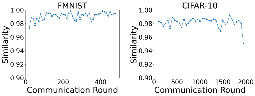
Figure 3: Covariance Stationarity in Non-IID FL [23]. Full experiment results and more details can be found in Sec. D.3.

Actually, the correlations between loss changes of different clients mainly arise from similarities between their datasets, which are invariant during the FL process. Thus, we hypothesise that the covariance also changes slowly in the concerned time range. To verify this, we use a large number of samples to evaluate the covariance 𝚺tsuperscript𝚺𝑡\bm{\Sigma}^{t} in each communication round, and calculate the cosine similarity between 𝚺tsuperscript𝚺𝑡\bm{\Sigma}^{t} and 𝚺t+Δtsuperscript𝚺𝑡Δ𝑡\bm{\Sigma}^{t+\Delta t}. We set Δt=10Δ𝑡10\Delta t=10 for FMNIST and Δt=50Δ𝑡50\Delta t=50 for CIFAR-10. As shown in Fig. 3, we can see that the similarity keeps very high (>0.97absent0.97>0.97 for FMNIST and >0.95absent0.95>0.95 for CIFAR-10) during the whole FL training process.

Accordingly, we do not need to update 𝑿tsuperscript𝑿𝑡{\bm{X}}^{t} in every round but inherit the embedding matrix 𝑿t1superscript𝑿𝑡1{\bm{X}}^{t-1} from the last round and train it only every ΔtΔ𝑡\Delta t rounds. Furthermore, we can reuse historical samples for GP training to reduce the number of samples S𝑆S that we need to collect in each GP training round. We summarize our update rule of 𝑿tsuperscript𝑿𝑡{\bm{X}}^{t} as follows:

𝑿t={𝑿t1,t%Δt0;argmax𝑿Φt(𝑿),t%Δt=0,superscript𝑿𝑡casessuperscript𝑿𝑡1percent𝑡Δ𝑡0otherwisesubscript𝑿subscriptΦ𝑡𝑿percent𝑡Δ𝑡0otherwise\displaystyle{\bm{X}}^{t}=\begin{cases}{\bm{X}}^{t-1},\quad t\%\Delta t\neq 0;\\ \mathop{\arg\max}_{\bm{X}}\Phi_{t}({\bm{X}}),\quad t\%\Delta t=0,\end{cases} (16)

where

Φt(𝑿)=m=0Mi=1Sγmlogp(Δ𝒍tmΔt(𝕊tmΔt,i)|𝑿).subscriptΦ𝑡𝑿superscriptsubscript𝑚0𝑀superscriptsubscript𝑖1𝑆superscript𝛾𝑚𝑝conditionalΔsuperscript𝒍𝑡𝑚Δ𝑡subscript𝕊𝑡𝑚Δ𝑡𝑖𝑿\displaystyle\Phi_{t}({\bm{X}})=\sum_{m=0}^{M}\sum_{i=1}^{S}\gamma^{m}\log p(\Delta\bm{l}^{t-m\Delta t}({\mathbb{S}}_{t-m\Delta t,i})|{\bm{X}}). (17)

M𝑀M is the number of reused historical samples, and γ<1𝛾1\gamma<1 is the discount factor to weight the historical samples. Our method is able to reduce the communication overhead with a large ΔtΔ𝑡\Delta t and S=1𝑆1S=1, while guaranteeing the performance.

As we only update the covariance 𝚺𝚺\bm{\Sigma} every ΔtΔ𝑡\Delta t rounds, the annealing factor βτksuperscript𝛽subscript𝜏𝑘\beta^{\tau_{k}} can prevent us from making the same selection during the ΔtΔ𝑡\Delta t rounds. Repeatedly training with the same group of clients would cause the global model to overfit on their data, which may hinder the convergence of FL. In practice, we reset τksubscript𝜏𝑘\tau_{k} to 00 after each GP training round to achieve the fastest convergence while avoiding overfitting on some clients.

We summarize our overall framework FedCor in Algorithm 2. It is noteworthy that our method is orthogonal to existing FL optimizers that amend the training loss or the aggregation scheme, e.g., FedAvg [23] and FedProx [18]. So our method can be combined with any of them.

5 Experiments
Refer to caption
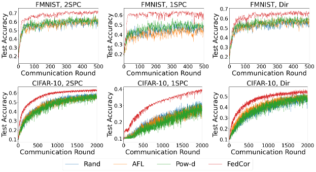
Figure 4: Test accuracy on FMNIST and CIFAR-10 under three heterogeneous settings (2SPC, 1SPC and Dir). All experiments in one figure share the same hyperparameters except for the client selection strategy.
Method FMNIST CIFAR-10
2SPC(69%percent6969\%) 1SPC(62%percent6262\%) Dir(64%percent6464\%) 2SPC(62%percent6262\%) 1SPC(36%percent3636\%) Dir(54%percent5454\%)
Rand 295.8±92.0plus-or-minus295.892.0295.8\pm 92.0 N/A 141.0±73.0plus-or-minus141.073.0141.0\pm 73.0 1561.2±236.2plus-or-minus1561.2236.21561.2\pm 236.2 1750.4±190.3plus-or-minus1750.4190.31750.4\pm 190.3 N/A
AFL 218.6±117.3plus-or-minus218.6117.3218.6\pm 117.3 N/A 169.0±166.1plus-or-minus169.0166.1169.0\pm 166.1 N/A 1845.2±28.8plus-or-minus1845.228.81845.2\pm 28.8 1524.4±267.9plus-or-minus1524.4267.91524.4\pm 267.9
Pow-d 126.6±78.2plus-or-minus126.678.2126.6\pm 78.2 167.2±72.3plus-or-minus167.272.3167.2\pm 72.3 123.0±101.0plus-or-minus123.0101.0123.0\pm 101.0 1558.2±227.0plus-or-minus1558.2227.01558.2\pm 227.0 1752.2±186.2plus-or-minus1752.2186.21752.2\pm 186.2 1355.2±151.3plus-or-minus1355.2151.31355.2\pm 151.3
FedCor (Ours) 94.8±18.4plus-or-minus94.818.4\bm{94.8\pm 18.4} 84.0±53.1plus-or-minus84.053.1\bm{84.0\pm 53.1} 68.8±27.5plus-or-minus68.827.5\bm{68.8\pm 27.5} 1033.4±123.7plus-or-minus1033.4123.7\bm{1033.4\pm 123.7} 1269.2±70.6plus-or-minus1269.270.6\bm{1269.2\pm 70.6} 1076.8±262.8plus-or-minus1076.8262.8\bm{1076.8\pm 262.8}
Table 1: The number of communication rounds for each selection strategy to achieve target test accuracies (specified in parentheses) under three heterogeneous settings (2SPC, 1SPC and Dir). The results consist of the mean and the standard deviation over 5 random seeds. N/A means that the corresponding selection strategy cannot achieve the target accuracy with some random seeds within the maximal number of communication rounds (500500500 for FMNIST and 200020002000 for CIFAR-10).

5.1 Experiment Settings

We conduct experiments on two datasets, FMNIST [34] and CIFAR-10 [14]. For FMNIST, we adopt an MLP model with two hidden layers, and this model achieves an accuracy of 85.92%percent85.9285.92\% with centralized training. For CIFAR-10, we adopt a CNN model with three convolutional layers followed by one fully connected layer, and this model can achieve an accuracy of 73.84%percent73.8473.84\% with centralized training. More details on the model construction and training hyperparameters can be found in Sec. C.1. For each dataset, we experiment with three different heterogeneous data partitions on N=100𝑁100N=100 clients as follows.

(i) 2 shards per client (2SPC): This setting is the same as the non-IID setting in [23]. We sort the data by their labels and divide them into 200200200 shards so that all the data in one shard share the same label. We randomly allocate these shards to clients, and each client has two shards. Since all the shards have the same size, the data partition is balanced. That is to say, all the clients have the same dataset size. We select C=5𝐶5C=5 clients in each round within this setting.

(ii) 1 shard per client (1SPC): This setting is similar to the 2SPC setting, and the only difference is that each client only has one shard, i.e., each client only has the data of one label. This is the data partition with the highest heterogeneity, and it is also balanced. We select C=10𝐶10C=10 clients in each round within this setting.

(iii) Dirichlet Distribution with α=0.2𝛼0.2\alpha=0.2 (Dir): We inherit and slightly change the setting from [7] to create an unbalanced data partition. We sample the ratio of the data with each label on one client from a Dirichlet Distribution parameterized by the concentration parameter α=0.2𝛼0.2\alpha=0.2. More details can be found in the Appendix C.2. We select C=5𝐶5C=5 clients in each round within this setting.

We divide the training process of FedCor into two phases: (i) Warm-up phase: We uniformly sample client selection 𝕂tsubscript𝕂𝑡{\mathbb{K}}_{t} and collect the loss values of all the clients in 𝕌𝕌{\mathbb{U}} to train the GP in each round, i.e., Δt=1Δ𝑡1\Delta t=1 and S=1𝑆1S=1. We set the length of the warm-up phase to 151515 for FMNIST and 202020 for CIFAR-10. (ii) Normal phase: After the warm-up phase, we follow Algorithm 2 to select clients and update the GP.

In all the experiments, we use FedAvg [23] as the FL optimizer. We present the average results using five random seeds in all experiments. We will first show that our method can achieve faster and more stable convergence, compared with three baselines: random selection (Rand), Active FL (AFL) [6] and Power-of-choice Selection Strategy (Pow-d) [4]. Then, we will give ablation studies on the GP training interval ΔtΔ𝑡\Delta t as well as the annealing coefficient β𝛽\beta. Finally, we visualize the client embeddings 𝑿𝑿{\bm{X}} with t-SNE [21] and show that FedCor can effectively capture the correlations.
Refer to caption
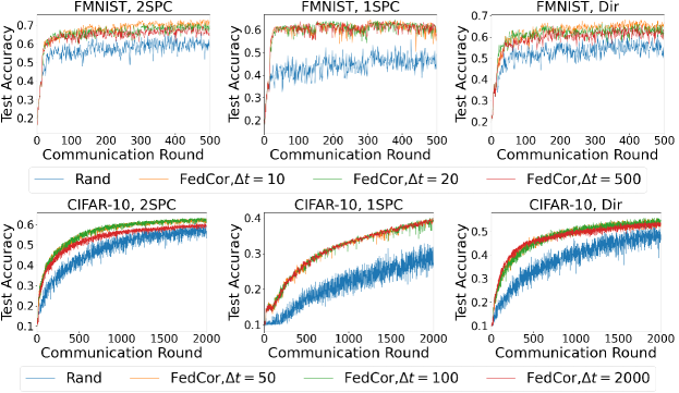
Figure 5: Test accuracy with different GP training interval ΔtΔ𝑡\Delta t on FMNIST and CIFAR-10 under 2SPC, 1SPC and Dir.

5.2 Convergence under Heterogeneous Settings

We compare the convergence rate of our method FedCor with the other baselines on both FMNIST and CIFAR-10, and demonstrate the results in Figure 4. We set the GP update interval Δt=10Δ𝑡10\Delta t=10 and the annealing coefficient β=0.95𝛽0.95\beta=0.95 for FMNIST experiments, and Δt=50Δ𝑡50\Delta t=50 and β=0.9𝛽0.9\beta=0.9 for CIFAR-10 experiments.

As shown in Figure 4, FedCor achieves the highest test accuracy and the fastest convergence in all experiments. While other active client selection strategies show only slight or even no superiority compared with the fully random strategy, our method clearly outperforms all baselines, especially under the extremely heterogeneous setting when data on each client contains only one label (1SPC). Furthermore, the learning curves of FedCor are more smooth and less noisy than those of other methods, meaning that FedCor reduces the variance and makes the federated optimization more stable.

Table 1 shows the numbers of communication rounds for each selection strategy to achieve a specified test accuracy. We can see that FedCor achieves the specified accuracy 34%99%similar-topercent34percent9934\%\sim 99\% and 26%51%similar-topercent26percent5126\%\sim 51\% faster than Pow-d on FMNIST and CIFAR-10, respectively.

5.3 Results with Larger GP Training Interval

Collecting training data in the GP update rounds brings communication overhead, since we need to broadcast the model to all the clients. Thus, it is important to investigate the minimal GP update frequency. We vary the GP training interval and show the accuracy curves in Figure 5. We set Δt=10,20,500Δ𝑡1020500\Delta t=10,20,500 with β=0.95,0.95,0.99𝛽0.950.950.99\beta=0.95,0.95,0.99 for the experiments on FMNIST, and Δt=50,100,2000Δ𝑡501002000\Delta t=50,100,2000 with β=0.97,0.97,0.999𝛽0.970.970.999\beta=0.97,0.97,0.999 for the experiments on CIFAR-10, respectively. As shown in the figures, the performance degrades very slightly with larger training intervals. It is noteworthy that even if we do not update the GP model after the warm-up phase (noted as Δt=500Δ𝑡500\Delta t=500 for FMNIST, and Δt=2000Δ𝑡2000\Delta t=2000 for CIFAR-10), FedCor still achieves faster convergence than the random selection strategy. These results indicate that the correlations learned by the GP model are stable, which supports our assumption in Section 4.5. In a word, one can largely reduce the communication overhead by training the GP model with a very low frequency while guaranteeing the convergence rate and accuracy under the communication-bounded FL setting.

5.4 Influence of Annealing Coefficient
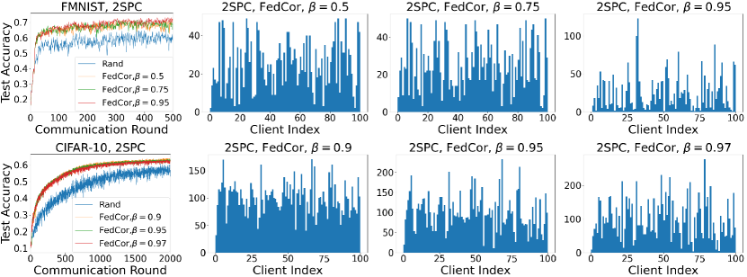
Refer to caption
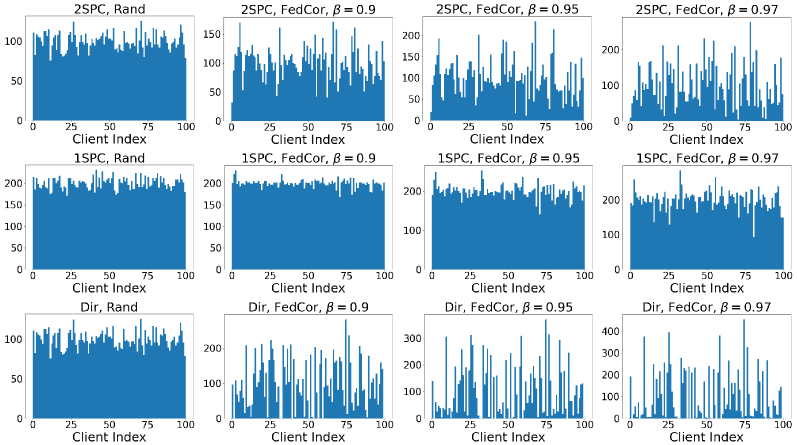
Figure 6: Test accuracy and client selection frequency with different annealing coefficient β𝛽\beta on FMNIST and CIFAR-10 under the 2SPC setting. The frequency is represented as the number of times each client is selected during the whole training process.

We also conduct experiments with different annealing coefficient β𝛽\beta that controls how “concentrated” the client selection is. We perform FedCor with Δt=10Δ𝑡10\Delta t=10 and β=0.5,0.75,0.9𝛽0.50.750.9\beta=0.5,0.75,0.9 for FMNIST, and Δt=50,β=0.9,0.95,0.99formulae-sequenceΔ𝑡50𝛽0.90.950.99\Delta t=50,\beta=0.9,0.95,0.99 for CIFAR-10. The learning curves as well as the client selection frequencies under 2SPC setting are shown in Fig. 6, and we leave the full results under the 1SPC and Dir settings to Sec. D.1. We observe that when using a smaller β𝛽\beta, the overall client selections appear to be more “uniform”, while the learning curves are almost invariant. Notice that this does not mean that FedCor with small β𝛽\beta is equivalent to uniform sampling, instead, FedCor still achieves consistent improvements compared to uniform sampling. And Sec. 4.4 havs discussed the reason: FedCor not only considers the benefit that each client brings to the federation, but also considers the correlations among the clients to select the best group of clients. The experimental results here show that it is more important to select a good “group” of clients than just good individuals.

5.5 Visualization of Client Embedding
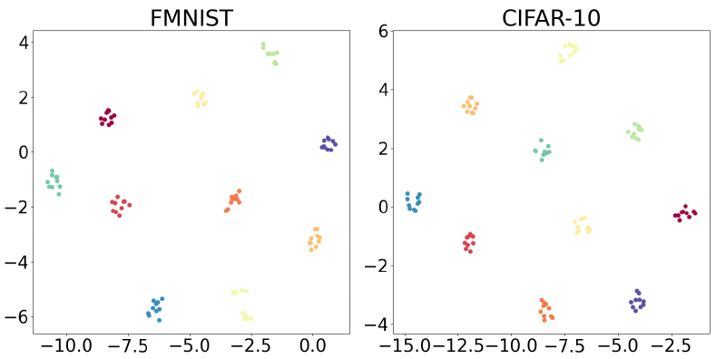
Refer to caption
Figure 7: Visualization of client embedding under the 1SPC setting.

To obtain an insight into the correlations learned by the GP model, we show the t-SNE [21] plot of the client embeddings learned in the warm-up phase under the 1SPC setting. In Fig. 7, each embedding is labeled with the only data label on the corresponding client. We normalize the length of embedding vectors to 111 so that the distance between two embeddings can reveal the correlation. We can see that the embeddings of clients with the same label are clustered together, which demonstrates that FedCor has captured the correlations between clients correctly in the warm-up phase.

6 Conclusion and Future Work

This work proposes FedCor, an FL framework with a novel client selection strategy for heterogeneous settings. FedCor is based on the intuition that it is crucial to utilize the correlations between clients to achieve a faster and more stable convergence in heterogeneous FL. Specifically, we model the client correlations with a GP, and design an effective and interpretable client selection strategy based on it. We also develop a efficient method to train the GP with a low communication overhead. Experimental results on FMNIST and CIFAR-10 show that FedCor effectively accelerates and stabilizes the training process under highly heterogeneous settings. In addition, we verify that FedCor captures the client correlation correctly using only the loss information. How to extend FedCor to the other tasks and further utilize the captured correlations is an interesting direction for future work. Besides, our method focuses on the cross-silo federated learning scenario [9], and how to extend it to the cross-device scenario is a meaningful topic.

Acknowledgement

This research was generously supported in part by Gift from Amazon, etc. Any opinions, conclusions or recommendations expressed in this material are those of the authors and do not reflect the views of Amazon and its contractors.

References

  • [1] Peter Auer. Using confidence bounds for exploitation-exploration trade-offs. Journal of Machine Learning Research, 3(Nov):397–422, 2002.
  • [2] Stephen Boyd, Neal Parikh, and Eric Chu. Distributed optimization and statistical learning via the alternating direction method of multipliers. Now Publishers Inc, 2011.
  • [3] Eric Brochu, Vlad M Cora, and Nando De Freitas. A tutorial on bayesian optimization of expensive cost functions, with application to active user modeling and hierarchical reinforcement learning. arXiv preprint arXiv:1012.2599, 2010.
  • [4] Yae Jee Cho, Jianyu Wang, and Gauri Joshi. Client selection in federated learning: Convergence analysis and power-of-choice selection strategies. arXiv preprint arXiv:2010.01243, 2020.
  • [5] Dennis D Cox and Susan John. A statistical method for global optimization. In [Proceedings] 1992 IEEE International Conference on Systems, Man, and Cybernetics, pages 1241–1246. IEEE, 1992.
  • [6] Jack Goetz, Kshitiz Malik, Duc Bui, Seungwhan Moon, Honglei Liu, and Anuj Kumar. Active federated learning. arXiv preprint arXiv:1909.12641, 2019.
  • [7] Tzu-Ming Harry Hsu, Hang Qi, and Matthew Brown. Measuring the effects of non-identical data distribution for federated visual classification. arXiv preprint arXiv:1909.06335, 2019.
  • [8] Tzu-Ming Harry Hsu, Hang Qi, and Matthew Brown. Federated visual classification with real-world data distribution. In Computer Vision–ECCV 2020: 16th European Conference, Glasgow, UK, August 23–28, 2020, Proceedings, Part X 16, pages 76–92. Springer, 2020.
  • [9] Peter Kairouz, H Brendan McMahan, Brendan Avent, Aurélien Bellet, Mehdi Bennis, Arjun Nitin Bhagoji, Keith Bonawitz, Zachary Charles, Graham Cormode, Rachel Cummings, et al. Advances and open problems in federated learning. arXiv preprint arXiv:1912.04977, 2019.
  • [10] Sai Praneeth Karimireddy, Satyen Kale, Mehryar Mohri, Sashank J Reddi, Sebastian U Stich, and Ananda Theertha Suresh. Scaffold: Stochastic controlled averaging for on-device federated learning. arXiv preprint arXiv:1910.06378, 2019.
  • [11] Diederik P Kingma and Jimmy Ba. Adam: A method for stochastic optimization. arXiv preprint arXiv:1412.6980, 2014.
  • [12] Jakub Konečnỳ, Brendan McMahan, and Daniel Ramage. Federated optimization: Distributed optimization beyond the datacenter. arXiv preprint arXiv:1511.03575, 2015.
  • [13] Jakub Konečnỳ, H Brendan McMahan, Felix X Yu, Peter Richtárik, Ananda Theertha Suresh, and Dave Bacon. Federated learning: Strategies for improving communication efficiency. arXiv preprint arXiv:1610.05492, 2016.
  • [14] Alex Krizhevsky, Geoffrey Hinton, et al. Learning multiple layers of features from tiny images. 2009.
  • [15] Ang Li, Jingwei Sun, Pengcheng Li, Yu Pu, Hai Li, and Yiran Chen. Hermes: an efficient federated learning framework for heterogeneous mobile clients. In Proceedings of the 27th Annual International Conference on Mobile Computing and Networking, pages 420–437, 2021.
  • [16] Ang Li, Jingwei Sun, Binghui Wang, Lin Duan, Sicheng Li, Yiran Chen, and Hai Li. Lotteryfl: Personalized and communication-efficient federated learning with lottery ticket hypothesis on non-iid datasets. arXiv preprint arXiv:2008.03371, 2020.
  • [17] Tian Li, Anit Kumar Sahu, Ameet Talwalkar, and Virginia Smith. Federated learning: Challenges, methods, and future directions. IEEE Signal Processing Magazine, 37(3):50–60, 2020.
  • [18] Tian Li, Anit Kumar Sahu, Manzil Zaheer, Maziar Sanjabi, Ameet Talwalkar, and Virginia Smith. Federated optimization in heterogeneous networks. arXiv preprint arXiv:1812.06127, 2018.
  • [19] Xiang Li, Kaixuan Huang, Wenhao Yang, Shusen Wang, and Zhihua Zhang. On the convergence of fedavg on non-iid data. arXiv preprint arXiv:1907.02189, 2019.
  • [20] Xianfeng Liang, Shuheng Shen, Jingchang Liu, Zhen Pan, Enhong Chen, and Yifei Cheng. Variance reduced local sgd with lower communication complexity. arXiv preprint arXiv:1912.12844, 2019.
  • [21] Laurens van der Maaten and Geoffrey Hinton. Visualizing data using t-sne. Journal of machine learning research, 9(Nov):2579–2605, 2008.
  • [22] Stephan Mandt, Matthew Hoffman, and David Blei. A variational analysis of stochastic gradient algorithms. In International conference on machine learning, pages 354–363, 2016.
  • [23] Brendan McMahan, Eider Moore, Daniel Ramage, Seth Hampson, and Blaise Aguera y Arcas. Communication-efficient learning of deep networks from decentralized data. In Artificial Intelligence and Statistics, pages 1273–1282. PMLR, 2017.
  • [24] Tomoya Murata and Taiji Suzuki. Bias-variance reduced local sgd for less heterogeneous federated learning. arXiv preprint arXiv:2102.03198, 2021.
  • [25] Amirhossein Reisizadeh, Farzan Farnia, Ramtin Pedarsani, and Ali Jadbabaie. Robust federated learning: The case of affine distribution shifts. arXiv preprint arXiv:2006.08907, 2020.
  • [26] Neta Shoham, Tomer Avidor, Aviv Keren, Nadav Israel, Daniel Benditkis, Liron Mor-Yosef, and Itai Zeitak. Overcoming forgetting in federated learning on non-iid data. arXiv preprint arXiv:1910.07796, 2019.
  • [27] Virginia Smith, Chao-Kai Chiang, Maziar Sanjabi, and Ameet S Talwalkar. Federated multi-task learning. In Advances in neural information processing systems, pages 4424–4434, 2017.
  • [28] Niranjan Srinivas, Andreas Krause, Sham M Kakade, and Matthias W Seeger. Information-theoretic regret bounds for gaussian process optimization in the bandit setting. IEEE Transactions on Information Theory, 58(5):3250–3265, 2012.
  • [29] TensorFlow team. Tensorflow convolutional neural networks tutorial. https://www.tensorflow.org/tutorials/images/cnn, 2016.
  • [30] Ngo Anh Vien, Heiko Zimmermann, and Marc Toussaint. Bayesian functional optimization. In Thirty-Second AAAI Conference on Artificial Intelligence, 2018.
  • [31] Jianyu Wang, Zachary Charles, Zheng Xu, Gauri Joshi, H Brendan McMahan, Maruan Al-Shedivat, Galen Andrew, Salman Avestimehr, Katharine Daly, Deepesh Data, et al. A field guide to federated optimization. arXiv preprint arXiv:2107.06917, 2021.
  • [32] Jianyu Wang, Qinghua Liu, Hao Liang, Gauri Joshi, and H Vincent Poor. Tackling the objective inconsistency problem in heterogeneous federated optimization. arXiv preprint arXiv:2007.07481, 2020.
  • [33] Christopher KI Williams and Carl Edward Rasmussen. Gaussian processes for machine learning, volume 2. MIT press Cambridge, MA, 2006.
  • [34] Han Xiao, Kashif Rasul, and Roland Vollgraf. Fashion-mnist: a novel image dataset for benchmarking machine learning algorithms. arXiv preprint arXiv:1708.07747, 2017.
  • [35] Tao Yang, Xinlei Yi, Junfeng Wu, Ye Yuan, Di Wu, Ziyang Meng, Yiguang Hong, Hong Wang, Zongli Lin, and Karl H Johansson. A survey of distributed optimization. Annual Reviews in Control, 47:278–305, 2019.

Appendix A Theoretical Analysis

A.1 Analytical Insight into Gaussian Processes

In this section, we give a mathematical explanation about why the loss changes obey Gaussian Distributions. Our analysis based on the following assumption where we assume that the global weight update in one communication round follow a Gaussian Distribution under uniformly client selection.

Assumption 1.

In any communication round t𝑡t, if the client selection 𝕂tsubscript𝕂𝑡{\mathbb{K}}_{t} is a random variable sampled from a uniform distribution, the global model update Δ𝐰t(𝕂t)=𝐰t+1(𝕂t)𝐰tΔsuperscript𝐰𝑡subscript𝕂𝑡superscript𝐰𝑡1subscript𝕂𝑡superscript𝐰𝑡\Delta{\mathbf{w}}^{t}({\mathbb{K}}_{t})={\mathbf{w}}^{t+1}({\mathbb{K}}_{t})-{\bm{w}}^{t} follows Gaussian Distribution, i.e.,

𝕂tUniform({𝕂𝕌:|𝕂|=C})similar-tosubscript𝕂𝑡Uniformconditional-set𝕂𝕌𝕂𝐶\displaystyle{\mathbb{K}}_{t}\sim{\rm Uniform}\big{(}\{{\mathbb{K}}\subseteq{\mathbb{U}}:|{\mathbb{K}}|=C\}\big{)} (18)
\displaystyle\Rightarrow Δ𝐰t(𝕂t)𝒩(Δ𝒘t;ηt𝒈~t,ηt2𝑩𝑩TC),similar-toΔsuperscript𝐰𝑡subscript𝕂𝑡𝒩Δsuperscript𝒘𝑡subscript𝜂𝑡superscript~𝒈𝑡superscriptsubscript𝜂𝑡2𝑩superscript𝑩𝑇𝐶\displaystyle\Delta{\mathbf{w}}^{t}({\mathbb{K}}_{t})\sim\mathcal{N}(\Delta{\bm{w}}^{t};-\eta_{t}\tilde{{\bm{g}}}^{t},\frac{\eta_{t}^{2}{\bm{B}}{\bm{B}}^{T}}{C}),

where 𝐠~t=𝔼k[~lk(𝐰t)]superscript~𝐠𝑡subscript𝔼kdelimited-[]~subscript𝑙ksuperscript𝐰𝑡\tilde{{\bm{g}}}^{t}=\mathbb{E}_{\textnormal{k}}[\tilde{\nabla}l_{\textnormal{k}}({\bm{w}}^{t})] is the mean cumulative gradient of all the clients in 𝕌𝕌{\mathbb{U}}, and 𝐁𝐁{\bm{B}} is a constant matrix.

Assumption 1 is inspired by [22] who assumes the stochastic gradients in SGD are Gaussian, and therefore the parameter update after one iteration follows a Gaussian Distribution. Note that in the FL procedure, the form in Eq. 5 is very similar to that in the SGD update. The only difference is that the average gradients within one mini-batch is replaced by the average cumulative gradients of the selected clients. Therefore, it is reasonable to make this assumption similar to [22].

To make a distinction, we use Δ𝐰Δ𝐰\Delta{\mathbf{w}} without parentheses to denote a random variable w.r.t. the uniformly sampled client selection, and use Δ𝒘(𝕂)Δ𝒘𝕂\Delta{\bm{w}}({\mathbb{K}}) to denote a determinate value without randomness where the client selection 𝕂𝕂{\mathbb{K}} is determined. The rule for Δ𝐥Δ𝐥\Delta{\mathbf{l}} and Δ𝒍(𝕂)Δ𝒍𝕂\Delta{\bm{l}}({\mathbb{K}}) in the following contents is the same.

Based on this assumption, we can easily show that the loss changes in each communication round follow a Gaussian Process under first-order approximation, with the property of Gaussian Distribution.

Corollary 1.

In any communication round t𝑡t, 𝕊={i1,,i|𝕊|}𝕌for-all𝕊subscript𝑖1subscript𝑖𝕊𝕌\forall{\mathbb{S}}=\{i_{1},\cdots,i_{|{\mathbb{S}}|}\}\subseteq{\mathbb{U}}, the loss changes Δ𝐥𝕊t=[Δli1t,,Δli|𝕊|t]TΔsuperscriptsubscript𝐥𝕊𝑡superscriptΔsuperscriptsubscriptlsubscript𝑖1𝑡Δsuperscriptsubscriptlsubscript𝑖𝕊𝑡𝑇\Delta{\mathbf{l}}_{\mathbb{S}}^{t}=[\Delta{\textnormal{l}}_{i_{1}}^{t},\cdots,\Delta{\textnormal{l}}_{i_{|{\mathbb{S}}|}}^{t}]^{T} follow a Multivariate Gaussian Distribution (or a Gaussian Process) under first-order approximation, i.e.,

Δ𝐥𝕊t𝒩(Δ𝒍𝕊t;𝝁𝕊t,𝚺𝕊t),similar-toΔsuperscriptsubscript𝐥𝕊𝑡𝒩Δsubscriptsuperscript𝒍𝑡𝕊superscriptsubscript𝝁𝕊𝑡superscriptsubscript𝚺𝕊𝑡\displaystyle\Delta{\mathbf{l}}_{{\mathbb{S}}}^{t}\sim\mathcal{N}(\Delta{\bm{l}}^{t}_{{\mathbb{S}}};\bm{\mu}_{{\mathbb{S}}}^{t},{\bm{\Sigma}}_{{\mathbb{S}}}^{t}), (19)
where
𝝁𝕊t=ηt𝑮𝕊tT𝒈~t;superscriptsubscript𝝁𝕊𝑡subscript𝜂𝑡superscriptsuperscriptsubscript𝑮𝕊𝑡𝑇superscript~𝒈𝑡\displaystyle\bm{\mu}_{{\mathbb{S}}}^{t}=-\eta_{t}{{\bm{G}}_{{\mathbb{S}}}^{t}}^{T}\tilde{{\bm{g}}}^{t};
𝚺𝕊t=ηt2C𝑮𝕊tT𝑩𝑩T𝑮𝕊t;superscriptsubscript𝚺𝕊𝑡superscriptsubscript𝜂𝑡2𝐶superscriptsuperscriptsubscript𝑮𝕊𝑡𝑇𝑩superscript𝑩𝑇superscriptsubscript𝑮𝕊𝑡\displaystyle{\bm{\Sigma}}_{{\mathbb{S}}}^{t}=\frac{\eta_{t}^{2}}{C}{{\bm{G}}_{{\mathbb{S}}}^{t}}^{T}{\bm{B}}{\bm{B}}^{T}{\bm{G}}_{{\mathbb{S}}}^{t};
𝑮𝕊t=[li1(𝒘t),,li|𝕊|(𝒘t)].superscriptsubscript𝑮𝕊𝑡matrixsubscript𝑙subscript𝑖1superscript𝒘𝑡subscript𝑙subscript𝑖𝕊superscript𝒘𝑡\displaystyle{\bm{G}}_{{\mathbb{S}}}^{t}=\begin{bmatrix}\nabla l_{i_{1}}({\bm{w}}^{t}),\cdots,\nabla l_{i_{|{{\mathbb{S}}}|}}({\bm{w}}^{t})\end{bmatrix}.

We remove the subscript 𝕊𝕊{\mathbb{S}} to simplify the corresponding representation for the client set 𝕌𝕌{\mathbb{U}} as

Δ𝐥t𝒩(Δ𝒍t;𝝁t,𝚺t),similar-toΔsuperscript𝐥𝑡𝒩Δsuperscript𝒍𝑡superscript𝝁𝑡superscript𝚺𝑡\Delta{\mathbf{l}}^{t}\sim\mathcal{N}(\Delta{\bm{l}}^{t};\bm{\mu}^{t},{\bm{\Sigma}}^{t}), (20)

which is exactly the result in Eq. 8. And we can also obtain a mathematical reason from Eq. 19 for our choice of homogeneous linear kernel in Section 4.5, where 𝑿t=𝑩T𝑮tsuperscript𝑿𝑡superscript𝑩𝑇superscript𝑮𝑡{\bm{X}}^{t}={\bm{B}}^{T}{\bm{G}}^{t}.

Remark

Although an uniformly sampled client selection is required in Assumption 1 to get the loss changes to follow a GP prior, it is not necessary for the final selection to be uniformly sampled since we are predicting its loss changes with the GP posterior conditioned on the selected clients. We can view each posterior during the iterative selection process in Section 4.3 as the distribution of the loss changes w.r.t. the client selection that consists of two parts: (i) fixed selected clients in the previous iteration and (ii) uniformly sampled clients from the rest of the clients.

A.2 Proof of Lemma 1

To prove Lemma 1, we first introduce another assumption.

Assumption 2.

In any communication round t𝑡t, for any client selection 𝕂𝕂{\mathbb{K}}, we have

Pr(𝕂|Δ𝒍𝕂t(𝕂))1.𝑃𝑟conditional𝕂Δsuperscriptsubscript𝒍𝕂𝑡𝕂1Pr({\mathbb{K}}|\Delta{\bm{l}}_{{\mathbb{K}}}^{t}({\mathbb{K}}))\approx 1. (21)

This assumption asserts that for any client selection 𝕂𝕂{\mathbb{K}}, there is unlikely another client selection other than 𝕂𝕂{\mathbb{K}} which can produce the same loss changes on 𝕂𝕂{\mathbb{K}}, i.e.,

𝕂,𝕂𝕌,|𝕂|=|𝕂|formulae-sequencefor-allsuperscript𝕂𝕂𝕌superscript𝕂𝕂\displaystyle\forall{\mathbb{K}}^{\prime},{\mathbb{K}}\subseteq{\mathbb{U}},|{\mathbb{K}}^{\prime}|=|{\mathbb{K}}| (22)
\displaystyle\Rightarrow Pr(Δ𝒍𝕂t(𝕂)=Δ𝒍𝕂t(𝕂)|𝕂𝕂)0.𝑃𝑟Δsuperscriptsubscript𝒍𝕂𝑡superscript𝕂conditionalΔsuperscriptsubscript𝒍𝕂𝑡𝕂superscript𝕂𝕂0\displaystyle Pr(\Delta{\bm{l}}_{{\mathbb{K}}}^{t}({\mathbb{K}}^{\prime})=\Delta{\bm{l}}_{{\mathbb{K}}}^{t}({\mathbb{K}})|{\mathbb{K}}^{\prime}\neq{\mathbb{K}})\approx 0.

We anticipate that this is a realistic assumption because of the heterogeneity between clients and the highly complexity of the neural network. When selecting different clients, the data used for training varies a lot under heterogeneous federated learning settings. This fact makes it almost impossible to produce the same neural network, and thus the same loss changes, with two different client selections. Furthermore, the selected clients usually have larger loss decreases than other clients who are not selected, because the model update is based on the mean cumulative gradient of these selected clients. The other client selection is unlikely to generate the same large loss decreases on all of them.

With Assumption 2, we can get the following corollary 2.

Corollary 2.

In any communication round t𝑡t, for any client selection 𝕂𝕂{\mathbb{K}}, we have

Pr(Δ𝒍t(𝕂)|Δ𝒍𝕂t(𝕂))1.𝑃𝑟conditionalΔsuperscript𝒍𝑡𝕂Δsuperscriptsubscript𝒍𝕂𝑡𝕂1Pr(\Delta{\bm{l}}^{t}({\mathbb{K}})|\Delta{\bm{l}}_{{\mathbb{K}}}^{t}({\mathbb{K}}))\approx 1. (23)
Proof.

When client selection 𝕂𝕂{\mathbb{K}} is given, we get the determinate model update Δ𝒘t(𝕂)Δsuperscript𝒘𝑡𝕂\Delta{\bm{w}}^{t}({\mathbb{K}}), thus the loss changes are known without randomness. In the other word,

Pr(Δ𝒍t(𝕂)|𝕂)=1𝑃𝑟conditionalΔsuperscript𝒍𝑡𝕂𝕂1Pr(\Delta{\bm{l}}^{t}({\mathbb{K}})|{\mathbb{K}})=1 (24)

always holds. Besides, we can extend the condition in Eq. 21 to the loss changes of all the clients and get

Pr(𝕂|Δ𝒍t(𝕂))1.𝑃𝑟conditional𝕂Δsuperscript𝒍𝑡𝕂1Pr({\mathbb{K}}|\Delta{\bm{l}}^{t}({\mathbb{K}}))\approx 1. (25)

Combining Eq. 21, Eq. 24 and Eq. 25, we have

Pr(Δ𝒍t(𝕂))𝑃𝑟Δsuperscript𝒍𝑡𝕂absent\displaystyle Pr(\Delta{\bm{l}}^{t}({\mathbb{K}}))\approx Pr(Δ𝒍t(𝕂),𝕂)𝑃𝑟Δsuperscript𝒍𝑡𝕂𝕂\displaystyle Pr(\Delta{\bm{l}}^{t}({\mathbb{K}}),{\mathbb{K}}) (26)
=\displaystyle= Pr(𝕂)𝑃𝑟𝕂\displaystyle Pr({\mathbb{K}}) (27)
=\displaystyle= Pr(Δ𝒍𝕂t(𝕂),𝕂)𝑃𝑟Δsuperscriptsubscript𝒍𝕂𝑡𝕂𝕂\displaystyle Pr(\Delta{\bm{l}}_{{\mathbb{K}}}^{t}({\mathbb{K}}),{\mathbb{K}}) (28)
\displaystyle\approx Pr(Δ𝒍𝕂t(𝕂))𝑃𝑟Δsuperscriptsubscript𝒍𝕂𝑡𝕂\displaystyle Pr(\Delta{\bm{l}}_{{\mathbb{K}}}^{t}({\mathbb{K}})) (29)

By substituting Eq. 29 into the expression of Pr(Δ𝒍t(𝕂)|Δ𝒍𝕂t(𝕂))𝑃𝑟conditionalΔsuperscript𝒍𝑡𝕂Δsuperscriptsubscript𝒍𝕂𝑡𝕂Pr(\Delta{\bm{l}}^{t}({\mathbb{K}})|\Delta{\bm{l}}_{{\mathbb{K}}}^{t}({\mathbb{K}})), we get

Pr(Δ𝒍t(𝕂)|Δ𝒍𝕂t(𝕂))=𝑃𝑟conditionalΔsuperscript𝒍𝑡𝕂Δsuperscriptsubscript𝒍𝕂𝑡𝕂absent\displaystyle Pr(\Delta{\bm{l}}^{t}({\mathbb{K}})|\Delta{\bm{l}}_{{\mathbb{K}}}^{t}({\mathbb{K}}))= Pr(Δ𝒍t(𝕂),Δ𝒍𝕂t(𝕂))Pr(Δ𝒍𝕂t(𝕂))𝑃𝑟Δsuperscript𝒍𝑡𝕂Δsuperscriptsubscript𝒍𝕂𝑡𝕂𝑃𝑟Δsuperscriptsubscript𝒍𝕂𝑡𝕂\displaystyle\frac{Pr(\Delta{\bm{l}}^{t}({\mathbb{K}}),\Delta{\bm{l}}_{{\mathbb{K}}}^{t}({\mathbb{K}}))}{Pr(\Delta{\bm{l}}_{{\mathbb{K}}}^{t}({\mathbb{K}}))} (30)
=\displaystyle= Pr(Δ𝒍t(𝕂))Pr(Δ𝒍𝕂t(𝕂))𝑃𝑟Δsuperscript𝒍𝑡𝕂𝑃𝑟Δsuperscriptsubscript𝒍𝕂𝑡𝕂\displaystyle\frac{Pr(\Delta{\bm{l}}^{t}({\mathbb{K}}))}{Pr(\Delta{\bm{l}}_{{\mathbb{K}}}^{t}({\mathbb{K}}))} (31)
\displaystyle\approx 1.1\displaystyle 1. (32)

Now we are ready to prove Lemma 1.

Lemma 1.

The optimization problem in Eq. 6 is approximately equivalent to the following probabilistic form.

min𝕂t𝔼Δ𝐥t|Δ𝒍𝕂tt(𝕂t)[ipiΔlit]=ipiμ~it(Δ𝒍𝕂tt(𝕂t)),subscriptsubscript𝕂𝑡subscript𝔼conditionalΔsuperscript𝐥𝑡Δsubscriptsuperscript𝒍𝑡subscript𝕂𝑡subscript𝕂𝑡delimited-[]subscript𝑖subscript𝑝𝑖Δsubscriptsuperscript𝑙𝑡𝑖subscript𝑖subscript𝑝𝑖subscriptsuperscript~𝜇𝑡𝑖Δsubscriptsuperscript𝒍𝑡subscript𝕂𝑡subscript𝕂𝑡\min_{{\mathbb{K}}_{t}}\quad\mathbb{E}_{\Delta{\mathbf{l}}^{t}|\Delta\bm{l}^{t}_{{\mathbb{K}}_{t}}({\mathbb{K}}_{t})}\Big{[}\sum_{i}p_{i}\Delta l^{t}_{i}\Big{]}=\sum_{i}p_{i}\tilde{\mu}^{t}_{i}(\Delta\bm{l}^{t}_{{\mathbb{K}}_{t}}({\mathbb{K}}_{t})), (33)

where Δ𝐥t=[Δl1t,,ΔlNt]Δsuperscript𝐥𝑡Δsubscriptsuperscriptl𝑡1Δsubscriptsuperscriptl𝑡𝑁\Delta{\mathbf{l}}^{t}=[\Delta{\textnormal{l}}^{t}_{1},\cdots,\Delta{\textnormal{l}}^{t}_{N}] is the loss changes of all clients in round t𝑡t, which is a random variable w.r.t random client selection in round t𝑡t. 𝛍~t(Δ𝐥𝕂tt(𝕂t))superscript~𝛍𝑡Δsubscriptsuperscript𝐥𝑡subscript𝕂𝑡subscript𝕂𝑡\tilde{\bm{\mu}}^{t}(\Delta\bm{l}^{t}_{{\mathbb{K}}_{t}}({\mathbb{K}}_{t})) is the posterior mean of Δ𝐥tΔsuperscript𝐥𝑡\Delta{\mathbf{l}}^{t} conditioned on Δ𝐥𝕂tt(𝕂t)=[Δlit(𝕂t)]i𝕂tΔsubscriptsuperscript𝐥𝑡subscript𝕂𝑡subscript𝕂𝑡subscriptdelimited-[]Δsubscriptsuperscript𝑙𝑡𝑖subscript𝕂𝑡𝑖subscript𝕂𝑡\Delta\bm{l}^{t}_{{\mathbb{K}}_{t}}({\mathbb{K}}_{t})=[\Delta l^{t}_{i}({\mathbb{K}}_{t})]_{i\in{\mathbb{K}}_{t}}.

Proof.

According to Corollary 2, we can transform the optimization problem in Eq. 6 into the form in Eq. 33.

min𝕂tΔLt(𝕂t)subscriptsubscript𝕂𝑡Δsuperscript𝐿𝑡subscript𝕂𝑡\displaystyle\min_{{\mathbb{K}}_{t}}\quad\Delta L^{t}({\mathbb{K}}_{t}) (34)
=\displaystyle= min𝕂tipiΔlit(𝕂t)subscriptsubscript𝕂𝑡subscript𝑖subscript𝑝𝑖Δsuperscriptsubscript𝑙𝑖𝑡subscript𝕂𝑡\displaystyle\min_{{\mathbb{K}}_{t}}\quad\sum_{i}p_{i}\Delta l_{i}^{t}({\mathbb{K}}_{t}) (35)
\displaystyle\approx min𝕂tPr(Δ𝒍t(𝕂t)|Δ𝒍𝕂tt(𝕂t))ipiΔlit(𝕂t)subscriptsubscript𝕂𝑡𝑃𝑟conditionalΔsuperscript𝒍𝑡subscript𝕂𝑡Δsuperscriptsubscript𝒍subscript𝕂𝑡𝑡subscript𝕂𝑡subscript𝑖subscript𝑝𝑖Δsuperscriptsubscript𝑙𝑖𝑡subscript𝕂𝑡\displaystyle\min_{{\mathbb{K}}_{t}}\quad Pr(\Delta{\bm{l}}^{t}({\mathbb{K}}_{t})|\Delta{\bm{l}}_{{\mathbb{K}}_{t}}^{t}({\mathbb{K}}_{t}))\sum_{i}p_{i}\Delta l_{i}^{t}({\mathbb{K}}_{t}) (36)
\displaystyle\approx min𝕂t𝔼Δ𝐥t|Δ𝒍𝕂tt(𝕂t)[ipiΔlit]subscriptsubscript𝕂𝑡subscript𝔼conditionalΔsuperscript𝐥𝑡Δsubscriptsuperscript𝒍𝑡subscript𝕂𝑡subscript𝕂𝑡delimited-[]subscript𝑖subscript𝑝𝑖Δsubscriptsuperscript𝑙𝑡𝑖\displaystyle\min_{{\mathbb{K}}_{t}}\quad\mathbb{E}_{\Delta{\mathbf{l}}^{t}|\Delta{\bm{l}}^{t}_{{\mathbb{K}}_{t}}({\mathbb{K}}_{t})}\Big{[}\sum_{i}p_{i}\Delta l^{t}_{i}\Big{]} (37)
=\displaystyle= min𝕂tipiμ~it(Δ𝒍𝕂tt(𝕂t)).subscriptsubscript𝕂𝑡subscript𝑖subscript𝑝𝑖subscriptsuperscript~𝜇𝑡𝑖Δsubscriptsuperscript𝒍𝑡subscript𝕂𝑡subscript𝕂𝑡\displaystyle\min_{{\mathbb{K}}_{t}}\quad\sum_{i}p_{i}\tilde{\mu}^{t}_{i}(\Delta{\bm{l}}^{t}_{{\mathbb{K}}_{t}}({\mathbb{K}}_{t})). (38)

A.3 Proof of Lemma 2

Lemma 2.

The selection criterion of FedCor when selecting two clients k1subscript𝑘1k_{1} and k2subscript𝑘2k_{2} can be written as

k1subscript𝑘1\displaystyle k_{1} =argmaxkβτkipiσirik,absentsubscript𝑘superscript𝛽subscript𝜏𝑘subscript𝑖subscript𝑝𝑖subscript𝜎𝑖subscript𝑟𝑖𝑘\displaystyle=\mathop{\arg\max}_{k}\quad\beta^{\tau_{k}}\sum_{i}p_{i}\sigma_{i}r_{ik}, (39)
k2subscript𝑘2\displaystyle k_{2} =argmaxkβτk[ipiσirikrk1kipiσirik1]1rkk12,absentsubscriptsuperscript𝑘superscript𝛽subscript𝜏superscript𝑘delimited-[]subscript𝑖subscript𝑝𝑖subscript𝜎𝑖subscript𝑟𝑖superscript𝑘subscript𝑟subscript𝑘1superscript𝑘subscript𝑖subscript𝑝𝑖subscript𝜎𝑖subscript𝑟𝑖subscript𝑘11superscriptsubscript𝑟superscript𝑘subscript𝑘12\displaystyle=\mathop{\arg\max}_{k^{\prime}}\quad\frac{\beta^{\tau_{k^{\prime}}}\Big{[}\sum_{i}p_{i}\sigma_{i}r_{ik^{\prime}}-r_{k_{1}k^{\prime}}\sum_{i}p_{i}\sigma_{i}r_{ik_{1}}\Big{]}}{\sqrt{1-r_{k^{\prime}k_{1}}^{2}}}, (40)

where rij=Σi,j/σiσjsubscript𝑟𝑖𝑗subscriptΣ𝑖𝑗subscript𝜎𝑖subscript𝜎𝑗r_{ij}=\Sigma_{i,j}/\sigma_{i}\sigma_{j} is the Pearson correlation coefficient.

Proof.

We first deduce Eq. 39 for the first client k1subscript𝑘1k_{1}. By substituting the loss change estimation Δl^kΔsubscript^𝑙𝑘\Delta\hat{l}_{k} from Eq. 9 into the criterion in Eq. 10, we can calculate the weighted sum of the posterior mean as

ipiμ~i(Δl^k)subscript𝑖subscript𝑝𝑖subscript~𝜇𝑖Δsubscript^𝑙𝑘\displaystyle\sum_{i}p_{i}\tilde{\mu}_{i}(\Delta\hat{l}_{k}) (41)
=\displaystyle= ipiμi+ipiΣi,kσk2(Δl^kμk)subscript𝑖subscript𝑝𝑖subscript𝜇𝑖subscript𝑖subscript𝑝𝑖subscriptΣ𝑖𝑘superscriptsubscript𝜎𝑘2Δsubscript^𝑙𝑘subscript𝜇𝑘\displaystyle\sum_{i}p_{i}\mu_{i}+\sum_{i}p_{i}\frac{\Sigma_{i,k}}{\sigma_{k}^{2}}(\Delta\hat{l}_{k}-\mu_{k}) (42)
=\displaystyle= ipiμiaβτkipiσirik,subscript𝑖subscript𝑝𝑖subscript𝜇𝑖𝑎superscript𝛽subscript𝜏𝑘subscript𝑖subscript𝑝𝑖subscript𝜎𝑖subscript𝑟𝑖𝑘\displaystyle\sum_{i}p_{i}\mu_{i}-a\beta^{\tau_{k}}\sum_{i}p_{i}\sigma_{i}r_{ik}, (43)

where riksubscript𝑟𝑖𝑘r_{ik} is the Pearson correlation coefficient. The first item in Eq. 43 and the factor a𝑎a are constant for all k𝑘k, thus the selection strategy becomes

k1=argmaxkβτkipiσirik,subscript𝑘1subscript𝑘superscript𝛽subscript𝜏𝑘subscript𝑖subscript𝑝𝑖subscript𝜎𝑖subscript𝑟𝑖𝑘k_{1}=\mathop{\arg\max}_{k}\quad\beta^{\tau_{k}}\sum_{i}p_{i}\sigma_{i}r_{ik}, (44)

which is Eq. 39.

Then we deduce Eq. 40 for selecting k2subscript𝑘2k_{2}. We can calculate the posterior covariance conditioned on Δl^k1Δsubscript^𝑙subscript𝑘1\Delta\hat{l}_{k_{1}} as

Σ~i,j(Δl^k1)subscript~Σ𝑖𝑗Δsubscript^𝑙subscript𝑘1\displaystyle\tilde{\Sigma}_{i,j}(\Delta\hat{l}_{k_{1}}) =Σi,jΣi,k1Σk1,jσk12absentsubscriptΣ𝑖𝑗subscriptΣ𝑖subscript𝑘1subscriptΣsubscript𝑘1𝑗superscriptsubscript𝜎subscript𝑘12\displaystyle=\Sigma_{i,j}-\frac{\Sigma_{i,k_{1}}\Sigma_{k_{1},j}}{\sigma_{k_{1}}^{2}} (45)
=σiσj(rijrik1rk1j)absentsubscript𝜎𝑖subscript𝜎𝑗subscript𝑟𝑖𝑗subscript𝑟𝑖subscript𝑘1subscript𝑟subscript𝑘1𝑗\displaystyle=\sigma_{i}\sigma_{j}(r_{ij}-r_{ik_{1}}r_{k_{1}j}) (46)
σ~i(Δl^k1)subscript~𝜎𝑖Δsubscript^𝑙subscript𝑘1\displaystyle\tilde{\sigma}_{i}(\Delta\hat{l}_{k_{1}}) =Σ~i,i(Δl^k1)absentsubscript~Σ𝑖𝑖Δsubscript^𝑙subscript𝑘1\displaystyle=\sqrt{\tilde{\Sigma}_{i,i}(\Delta\hat{l}_{k_{1}})} (47)
=σi1rik12.absentsubscript𝜎𝑖1superscriptsubscript𝑟𝑖subscript𝑘12\displaystyle=\sigma_{i}\sqrt{1-r_{ik_{1}}^{2}}. (48)

We substitute the posterior covariance into the simplified selection criterion in Eq. 44 and get

βτkipiΣ~i,k(Δl^k1)σ~k(Δl^k1)superscript𝛽subscript𝜏superscript𝑘subscript𝑖subscript𝑝𝑖subscript~Σ𝑖superscript𝑘Δsubscript^𝑙subscript𝑘1subscript~𝜎superscript𝑘Δsubscript^𝑙subscript𝑘1\displaystyle\beta^{\tau_{k^{\prime}}}\sum_{i}p_{i}\frac{\tilde{\Sigma}_{i,k^{\prime}}(\Delta\hat{l}_{k_{1}})}{\tilde{\sigma}_{k^{\prime}}(\Delta\hat{l}_{k_{1}})} (49)
=\displaystyle= βτk[ipiσirikrk1kipiσirik1]1rkk12.superscript𝛽subscript𝜏superscript𝑘delimited-[]subscript𝑖subscript𝑝𝑖subscript𝜎𝑖subscript𝑟𝑖superscript𝑘subscript𝑟subscript𝑘1superscript𝑘subscript𝑖subscript𝑝𝑖subscript𝜎𝑖subscript𝑟𝑖subscript𝑘11superscriptsubscript𝑟superscript𝑘subscript𝑘12\displaystyle\frac{\beta^{\tau_{k^{\prime}}}\Big{[}\sum_{i}p_{i}\sigma_{i}r_{ik^{\prime}}-r_{k_{1}k^{\prime}}\sum_{i}p_{i}\sigma_{i}r_{ik_{1}}\Big{]}}{\sqrt{1-r_{k^{\prime}k_{1}}^{2}}}.

So we have Eq. 40:

k2=argmaxkβτk[ipiσirikrk1kipiσirik1]1rkk12.subscript𝑘2subscriptsuperscript𝑘superscript𝛽subscript𝜏superscript𝑘delimited-[]subscript𝑖subscript𝑝𝑖subscript𝜎𝑖subscript𝑟𝑖superscript𝑘subscript𝑟subscript𝑘1superscript𝑘subscript𝑖subscript𝑝𝑖subscript𝜎𝑖subscript𝑟𝑖subscript𝑘11superscriptsubscript𝑟superscript𝑘subscript𝑘12k_{2}=\mathop{\arg\max}_{k^{\prime}}\quad\frac{\beta^{\tau_{k^{\prime}}}\Big{[}\sum_{i}p_{i}\sigma_{i}r_{ik^{\prime}}-r_{k_{1}k^{\prime}}\sum_{i}p_{i}\sigma_{i}r_{ik_{1}}\Big{]}}{\sqrt{1-r_{k^{\prime}k_{1}}^{2}}}. (50)

Appendix B Selection Criterion and Convergence Analysis

In this section, we will analyse FedCor when selecting arbitrary number of clients. While the iterative client selection makes it obscure to analyse the convergence, we will show that we can construct a simpler proxy algorithm who can approximate the selection strategy of FedCor and there for share similar convergence characteristic. We will prove the convergence of this proxy algorithm.

B.1 Definitions

We first introduce some important definitions. In the following analysis, We denote the client selection sampled from FedCor as 𝕂tπsimilar-tosubscript𝕂𝑡𝜋{\mathbb{K}}_{t}\sim\pi and client selection sampled uniformly as 𝕂t𝒰similar-tosubscript𝕂𝑡𝒰{\mathbb{K}}_{t}\sim\mathcal{U}.

In the j𝑗j-th iteration of FedCor, we select a client kjsubscript𝑘𝑗k_{j} to minimize the posterior mean of the loss change. Since the prior mean in each iteration is fixed, we can say that we are maximizing the decrease from prior mean 𝝁t,jsuperscript𝝁𝑡𝑗\bm{\mu}^{t,j} to posterior mean 𝝁~t,jsuperscript~𝝁𝑡𝑗\tilde{\bm{\mu}}^{t,j}. We define the posterior gain of this iteration as the decrease from prior mean to posterior mean, namely,

gt,j(kj)superscript𝑔𝑡𝑗subscript𝑘𝑗\displaystyle g^{t,j}(k_{j}) =ipi(μit,jμ~it,j(Δl^kjt))absentsubscript𝑖subscript𝑝𝑖subscriptsuperscript𝜇𝑡𝑗𝑖subscriptsuperscript~𝜇𝑡𝑗𝑖Δsubscriptsuperscript^𝑙𝑡subscript𝑘𝑗\displaystyle=\sum_{i}p_{i}(\mu^{t,j}_{i}-\tilde{\mu}^{t,j}_{i}(\Delta\hat{l}^{t}_{k_{j}})) (51)
=αkjtipiσit,jrikjt,j.absentsuperscriptsubscript𝛼subscript𝑘𝑗𝑡subscript𝑖subscript𝑝𝑖superscriptsubscript𝜎𝑖𝑡𝑗superscriptsubscript𝑟𝑖subscript𝑘𝑗𝑡𝑗\displaystyle=\alpha_{k_{j}}^{t}\sum_{i}p_{i}\sigma_{i}^{t,j}r_{ik_{j}}^{t,j}. (52)

We define 𝝁t,1=𝝁tsuperscript𝝁𝑡1superscript𝝁𝑡\bm{\mu}^{t,1}=\bm{\mu}^{t} and 𝚺t,1=𝚺tsuperscript𝚺𝑡1superscript𝚺𝑡\bm{\Sigma}^{t,1}=\bm{\Sigma}^{t}. And for j>1𝑗1j>1 we have

𝝁t,j=𝝁~t,j1(Δl^kj1t),𝚺t,j=𝚺~t,j1(Δl^kj1t).formulae-sequencesuperscript𝝁𝑡𝑗superscript~𝝁𝑡𝑗1Δsubscriptsuperscript^𝑙𝑡subscript𝑘𝑗1superscript𝚺𝑡𝑗superscript~𝚺𝑡𝑗1Δsubscriptsuperscript^𝑙𝑡subscript𝑘𝑗1\displaystyle\bm{\mu}^{t,j}=\tilde{\bm{\mu}}^{t,j-1}(\Delta\hat{l}^{t}_{k_{j-1}}),\qquad\bm{\Sigma}^{t,j}=\tilde{\bm{\Sigma}}^{t,j-1}(\Delta\hat{l}^{t}_{k_{j-1}}). (53)

With Lemma 2, we get

gt,j(kj)=gt,j1(kj)αkjtαkj1trkj1kjt,j1gt,j1(kj1)1rkj1kjt,j12.superscript𝑔𝑡𝑗subscript𝑘𝑗superscript𝑔𝑡𝑗1subscript𝑘𝑗superscriptsubscript𝛼subscript𝑘𝑗𝑡superscriptsubscript𝛼subscript𝑘𝑗1𝑡subscriptsuperscript𝑟𝑡𝑗1subscript𝑘𝑗1subscript𝑘𝑗superscript𝑔𝑡𝑗1subscript𝑘𝑗11superscriptsubscriptsuperscript𝑟𝑡𝑗1subscript𝑘𝑗1subscript𝑘𝑗2\displaystyle g^{t,j}(k_{j})=\frac{g^{t,j-1}(k_{j})-\frac{\alpha_{k_{j}}^{t}}{\alpha_{k_{j-1}}^{t}}r^{t,j-1}_{k_{j-1}k_{j}}g^{t,j-1}(k_{j-1})}{\sqrt{1-{r^{t,j-1}_{k_{j-1}k_{j}}}^{2}}}. (54)

With this notation, we can simplify our selection strategy as follows.

kj=argmaxkjgt,j(kj).superscriptsubscript𝑘𝑗subscriptsubscript𝑘𝑗superscript𝑔𝑡𝑗subscript𝑘𝑗\displaystyle k_{j}^{*}=\mathop{\arg\max}_{k_{j}}g^{t,j}(k_{j}). (55)

We further define the one-round advantage of FedCor compared with uniform sampling as follows.

At=superscript𝐴𝑡absent\displaystyle A^{t}= 𝔼𝕂t𝒰[L(𝒘t+1)L(𝒘t)]limit-fromsubscript𝔼similar-tosubscript𝕂𝑡𝒰delimited-[]𝐿superscript𝒘𝑡1𝐿superscript𝒘𝑡\displaystyle\mathbb{E}_{{\mathbb{K}}_{t}\sim\mathcal{U}}[L({\bm{w}}^{t+1})-L({\bm{w}}^{t})]-
𝔼𝕂tπ[L(𝒘t+1)L(𝒘t)]subscript𝔼similar-tosubscript𝕂𝑡𝜋delimited-[]𝐿superscript𝒘𝑡1𝐿superscript𝒘𝑡\displaystyle\mathbb{E}_{{\mathbb{K}}_{t}\sim\pi}[L({\bm{w}}^{t+1})-L({\bm{w}}^{t})] (56)
=\displaystyle= j=1Cgt,j(kj).superscriptsubscript𝑗1𝐶superscript𝑔𝑡𝑗superscriptsubscript𝑘𝑗\displaystyle\sum_{j=1}^{C}g^{t,j}(k_{j}^{*}). (57)

The second equation directly arises from the definition of our prior distribution where 𝔼𝕂t𝒰[L(𝒘t+1)L(𝒘t)]=iμitsubscript𝔼similar-tosubscript𝕂𝑡𝒰delimited-[]𝐿superscript𝒘𝑡1𝐿superscript𝒘𝑡subscript𝑖superscriptsubscript𝜇𝑖𝑡\mathbb{E}_{{\mathbb{K}}_{t}\sim\mathcal{U}}[L({\bm{w}}^{t+1})-L({\bm{w}}^{t})]=\sum_{i}\mu_{i}^{t}.

Unfortunately, because of the iterative selection, the selection criterion of kjsubscript𝑘𝑗k_{j} depends on the previous selected clients, which makes a quantitatively analysis complicated. To bypass this difficulty, we will first point out that Atsuperscript𝐴𝑡A^{t} has a lower bound that is tight in some special cases. We find that a proxy client selection strategy that maximizes this lower bound has a similar but simpler behaviour compared with FedCor, and we will also give a convergence guarantee of the proxy algorithm.

B.2 Approximation of FedCor

An important property of FedCor is that it prefers clients who have lower correlations with those selected in the previous iteration, since

rkj1kjt,j1(1,1),gt,j(kj)rkj1kjt,j1<0.formulae-sequencefor-allsubscriptsuperscript𝑟𝑡𝑗1subscript𝑘𝑗1subscript𝑘𝑗11superscript𝑔𝑡𝑗subscript𝑘𝑗subscriptsuperscript𝑟𝑡𝑗1subscript𝑘𝑗1subscript𝑘𝑗0\forall r^{t,j-1}_{k_{j-1}k_{j}}\in(-1,1),\frac{\partial g^{t,j}(k_{j})}{\partial r^{t,j-1}_{k_{j-1}k_{j}}}<0. (58)

We further predict that FedCor tends to select clients that with rkj1kjt,j1subscriptsuperscript𝑟𝑡𝑗1subscript𝑘𝑗1subscript𝑘𝑗r^{t,j-1}_{k_{j-1}k_{j}} close to 00 instead of rkj1kjt,j1<0subscriptsuperscript𝑟𝑡𝑗1subscript𝑘𝑗1subscript𝑘𝑗0r^{t,j-1}_{k_{j-1}k_{j}}<0 because if rkj1kjt,j1<0subscriptsuperscript𝑟𝑡𝑗1subscript𝑘𝑗1subscript𝑘𝑗0r^{t,j-1}_{k_{j-1}k_{j}}<0, kjsubscript𝑘𝑗k_{j} should be far away from kj1subscript𝑘𝑗1k_{j-1} who is closed to other clients in the embedding space, which makes kjsubscript𝑘𝑗k_{j} has low correlation with the other clients and not be selected. Therefore, we can infer that FedCor will select a group of clients who have nearly zero correlations with each other, which simplifies the expression of gt,j(kj)superscript𝑔𝑡𝑗subscript𝑘𝑗g^{t,j}(k_{j}) to gt,1(kj)superscript𝑔𝑡1subscript𝑘𝑗g^{t,1}(k_{j}).

Based on the analysis above, we define a proxy algorithm π~~𝜋\tilde{\pi} who maximize the following objective.

A~t=kj𝕂tCgt,1(kj)k𝕂tipiΣi,kt,superscript~𝐴𝑡superscriptsubscriptsubscript𝑘𝑗subscript𝕂𝑡𝐶superscript𝑔𝑡1subscript𝑘𝑗subscript𝑘subscript𝕂𝑡subscript𝑖subscript𝑝𝑖subscriptsuperscriptΣ𝑡𝑖𝑘\displaystyle\tilde{A}^{t}=\sum_{k_{j}\in{\mathbb{K}}_{t}}^{C}g^{t,1}(k_{j})\approx\sum_{k\in{\mathbb{K}}_{t}}\sum_{i}p_{i}\Sigma^{t}_{i,k}, (59)

where we further omit the difference of αktsuperscriptsubscript𝛼𝑘𝑡\alpha_{k}^{t} and σktsuperscriptsubscript𝜎𝑘𝑡\sigma_{k}^{t} for different client k𝑘k. We can use the client selection generated by this proxy algorithm to approximate the client selection of FedCor, and thus they share similar convergence characteristic.

In the following section, we will show that this proxy algorithm has a good property that enable it to converge to the optimal solution of the global loss L𝐿L without gap, even it is a biased selection strategy.

B.3 Convergence Analysis of the Proxy Algorithm

In the following section, we denote the client selection sampled from the proxy client selection strategy as 𝕂tπ~similar-tosubscript𝕂𝑡~𝜋{\mathbb{K}}_{t}\sim\tilde{\pi}. We use 𝔼[]𝔼delimited-[]\mathbb{E}[\cdot] as the expectation over the mini-batch and 𝔼𝕂t[]subscript𝔼subscript𝕂𝑡delimited-[]\mathbb{E}_{{\mathbb{K}}_{t}}[\cdot] as the expectation over the client selection strategy. We first give the common assumptions used in Federated Learning [19, 4].

Assumption 3.

l1,l2,,lNsubscript𝑙1subscript𝑙2subscript𝑙𝑁l_{1},l_{2},\cdots,l_{N} are all M𝑀M-smooth: for all 𝐯𝐯{\bm{v}} and 𝐰𝐰{\bm{w}}, lk(𝐯)lk(𝐰)+(𝐯𝐰)Tlk(𝐰)+M2𝐯𝐰22subscript𝑙𝑘𝐯subscript𝑙𝑘𝐰superscript𝐯𝐰𝑇subscript𝑙𝑘𝐰𝑀2superscriptsubscriptnorm𝐯𝐰22l_{k}({\bm{v}})\leq l_{k}({\bm{w}})+({\bm{v}}-{\bm{w}})^{T}\nabla l_{k}({\bm{w}})+\frac{M}{2}\Arrowvert{\bm{v}}-{\bm{w}}\Arrowvert_{2}^{2}.

Assumption 4.

l1,l2,,lNsubscript𝑙1subscript𝑙2subscript𝑙𝑁l_{1},l_{2},\cdots,l_{N} are all m𝑚m-strongly convex: for all 𝐯𝐯{\bm{v}} and 𝐰𝐰{\bm{w}}, lk(𝐯)lk(𝐰)+(𝐯𝐰)Tlk(𝐰)+m2𝐯𝐰22subscript𝑙𝑘𝐯subscript𝑙𝑘𝐰superscript𝐯𝐰𝑇subscript𝑙𝑘𝐰𝑚2superscriptsubscriptnorm𝐯𝐰22l_{k}({\bm{v}})\geq l_{k}({\bm{w}})+({\bm{v}}-{\bm{w}})^{T}\nabla l_{k}({\bm{w}})+\frac{m}{2}\Arrowvert{\bm{v}}-{\bm{w}}\Arrowvert_{2}^{2}.

Assumption 5.

For the mini-batch ξk𝔻ksubscript𝜉𝑘subscript𝔻𝑘\xi_{k}\in{\mathbb{D}}_{k} sampled uniformly on each client k𝕌𝑘𝕌k\in{\mathbb{U}}, the variance of stochastic gradients is bounded: 𝔼lk(𝐰k,ξk)lk(𝐰k)2sk2𝔼superscriptnormsubscript𝑙𝑘subscript𝐰𝑘subscript𝜉𝑘subscript𝑙𝑘subscript𝐰𝑘2superscriptsubscript𝑠𝑘2\mathbb{E}\Arrowvert\nabla l_{k}({\bm{w}}_{k},\xi_{k})-\nabla l_{k}({\bm{w}}_{k})\Arrowvert^{2}\leq s_{k}^{2}.

Assumption 6.

For each client k𝕌𝑘𝕌k\in{\mathbb{U}} and any communication round t𝑡t, the expected squared norm of stochastic gradients is uniformly bounded: 𝔼lk(𝐰k,ξk)2G2𝔼superscriptnormsubscript𝑙𝑘subscript𝐰𝑘subscript𝜉𝑘2superscript𝐺2\mathbb{E}\Arrowvert\nabla l_{k}({\bm{w}}_{k},\xi_{k})\Arrowvert^{2}\leq G^{2}.

For concision, we omit 𝔼𝔼\mathbb{E} in the following content and apply an expectation over the mini-batch by default.

Now we give an important property of the proxy algorithm that will be used for proving the convergence.

Lemma 3.

In any communication round t𝑡t, with Assumption 1 and Assumption 2 holds, we have

𝕂tπ~=argmax𝕂(𝑩TL(𝒘t))Tk𝕂𝑩Tlk(𝒘t).similar-tosubscript𝕂𝑡~𝜋subscript𝕂superscriptsuperscript𝑩𝑇𝐿superscript𝒘𝑡𝑇subscript𝑘𝕂superscript𝑩𝑇subscript𝑙𝑘superscript𝒘𝑡\displaystyle{\mathbb{K}}_{t}\sim\tilde{\pi}=\mathop{\arg\max}_{{\mathbb{K}}}({\bm{B}}^{T}\nabla L({\bm{w}}^{t}))^{T}\sum_{k\in{\mathbb{K}}}{\bm{B}}^{T}\nabla l_{k}({\bm{w}}^{t}). (60)
Proof.

In the proxy algorithm, we have

𝕂t=subscript𝕂𝑡absent\displaystyle{\mathbb{K}}_{t}= argmax𝕂k𝕂tipiΣi,ktsubscript𝕂subscript𝑘subscript𝕂𝑡subscript𝑖subscript𝑝𝑖subscriptsuperscriptΣ𝑡𝑖𝑘\displaystyle\mathop{\arg\max}_{{\mathbb{K}}}\sum_{k\in{\mathbb{K}}_{t}}\sum_{i}p_{i}\Sigma^{t}_{i,k} (61)
=\displaystyle= argmax𝕂ηt2Ck𝕂ipili(𝒘t)𝑩𝑩Tlk(𝒘t)subscript𝕂subscriptsuperscript𝜂2𝑡𝐶subscript𝑘𝕂subscript𝑖subscript𝑝𝑖subscript𝑙𝑖superscript𝒘𝑡𝑩superscript𝑩𝑇subscript𝑙𝑘superscript𝒘𝑡\displaystyle\mathop{\arg\max}_{{\mathbb{K}}}\frac{\eta^{2}_{t}}{C}\sum_{k\in{\mathbb{K}}}\sum_{i}p_{i}\nabla l_{i}({\bm{w}}^{t}){\bm{B}}{\bm{B}}^{T}\nabla l_{k}({\bm{w}}^{t}) (62)
=\displaystyle= argmax𝕂(𝑩TL(𝒘t))Tk𝕂𝑩Tlk(𝒘t).subscript𝕂superscriptsuperscript𝑩𝑇𝐿superscript𝒘𝑡𝑇subscript𝑘𝕂superscript𝑩𝑇subscript𝑙𝑘superscript𝒘𝑡\displaystyle\mathop{\arg\max}_{{\mathbb{K}}}({\bm{B}}^{T}\nabla L({\bm{w}}^{t}))^{T}\sum_{k\in{\mathbb{K}}}{\bm{B}}^{T}\nabla l_{k}({\bm{w}}^{t}). (63)

Eq. 62 comes from the expression of 𝚺tsuperscript𝚺𝑡\bm{\Sigma}^{t} in Corollary 1, and Eq. 63 arises from L(𝒘t)=ipili(𝒘t)𝐿superscript𝒘𝑡subscript𝑖subscript𝑝𝑖subscript𝑙𝑖superscript𝒘𝑡L({\bm{w}}^{t})=\sum_{i}p_{i}l_{i}({\bm{w}}^{t}). ∎

To connect this property with the convergence of the algorithm, we first define a sequence and show that the convergence of this sequence is equivalent to the convergence of the algorithm with this property. We define Sequence ΔtsubscriptΔ𝑡\Delta_{t} as follows.

Δt=𝔼𝕂tπ~𝒘t𝒘𝕂t2,subscriptΔ𝑡subscript𝔼similar-tosubscript𝕂𝑡~𝜋superscriptnormsuperscript𝒘𝑡superscriptsubscript𝒘subscript𝕂𝑡2\displaystyle\Delta_{t}=\mathbb{E}_{{\mathbb{K}}_{t}\sim\tilde{\pi}}\Arrowvert{\bm{w}}^{t}-{\bm{w}}_{{\mathbb{K}}_{t}}^{*}\Arrowvert^{2}, (64)
where
𝒘𝕂t=argmin𝒘k𝕂tlk(𝒘).superscriptsubscript𝒘subscript𝕂𝑡subscript𝒘subscript𝑘subscript𝕂𝑡subscript𝑙𝑘𝒘\displaystyle{\bm{w}}_{{\mathbb{K}}_{t}}^{*}=\mathop{\arg\min}_{{\bm{w}}}\sum_{k\in{\mathbb{K}}_{t}}l_{k}({\bm{w}}). (65)

We now show that if Δt0subscriptΔ𝑡0\Delta_{t}\rightarrow 0, we have 𝒘𝒘𝒘superscript𝒘{\bm{w}}\rightarrow{\bm{w}}^{*}.

Corollary 3.

(Optimal Solution Consistency) If ΔtsubscriptΔt\Delta_{t} converges to 00, there must be 𝐰tsuperscript𝐰t{\bm{w}}^{t} converges to 𝐰superscript𝐰{\bm{w}}^{*}.

limtΔt=0limt𝒘t=𝒘subscript𝑡subscriptΔ𝑡0subscript𝑡superscript𝒘𝑡superscript𝒘\displaystyle\lim_{t\rightarrow\infty}\Delta_{t}=0\Rightarrow\lim_{t\rightarrow\infty}{\bm{w}}^{t}={\bm{w}}^{*} (66)
Proof.

With 𝕂tπ~similar-tosubscript𝕂𝑡~𝜋{\mathbb{K}}_{t}\sim\tilde{\pi}, we have

limtΔt=0subscript𝑡subscriptΔ𝑡0\displaystyle\lim_{t\rightarrow\infty}\Delta_{t}=0 (67)
\displaystyle\Rightarrow limt𝒘t=𝒘𝕂tsubscript𝑡superscript𝒘𝑡superscriptsubscript𝒘subscript𝕂𝑡\displaystyle\lim_{t\rightarrow\infty}{\bm{w}}^{t}={\bm{w}}_{{\mathbb{K}}_{t}}^{*} (68)
\displaystyle\Rightarrow limtk𝕂tlk(𝒘t)=𝟎subscript𝑡subscript𝑘subscript𝕂𝑡subscript𝑙𝑘superscript𝒘𝑡0\displaystyle\lim_{t\rightarrow\infty}\sum_{k\in{\mathbb{K}}_{t}}\nabla l_{k}({\bm{w}}^{t})=\bm{0} (69)
\displaystyle\Rightarrow limt(𝑩TL(𝒘t))Tk𝕂t𝑩Tlk(𝒘t)=0.subscript𝑡superscriptsuperscript𝑩𝑇𝐿superscript𝒘𝑡𝑇subscript𝑘subscript𝕂𝑡superscript𝑩𝑇subscript𝑙𝑘superscript𝒘𝑡0\displaystyle\lim_{t\rightarrow\infty}({\bm{B}}^{T}\nabla L({\bm{w}}^{t}))^{T}\sum_{k\in{\mathbb{K}}_{t}}{\bm{B}}^{T}\nabla l_{k}({\bm{w}}^{t})=0. (70)

Since

𝕂t=argmax𝕂(𝑩TL(𝒘t))Tk𝕂𝑩Tlk(𝒘t),subscript𝕂𝑡subscript𝕂superscriptsuperscript𝑩𝑇𝐿superscript𝒘𝑡𝑇subscript𝑘𝕂superscript𝑩𝑇subscript𝑙𝑘superscript𝒘𝑡\displaystyle{\mathbb{K}}_{t}=\mathop{\arg\max}_{{\mathbb{K}}}({\bm{B}}^{T}\nabla L({\bm{w}}^{t}))^{T}\sum_{k\in{\mathbb{K}}}{\bm{B}}^{T}\nabla l_{k}({\bm{w}}^{t}), (71)

If limt𝑩TL(𝒘t)𝟎subscript𝑡superscript𝑩𝑇𝐿superscript𝒘𝑡0\lim_{t\rightarrow\infty}{\bm{B}}^{T}\nabla L({\bm{w}}^{t})\neq\bm{0} or does not converge, we can say that

ϵ>0,τ,t>τ,𝕂,formulae-sequencefor-allitalic-ϵ0𝜏for-all𝑡𝜏for-all𝕂\displaystyle\forall\epsilon>0,\exists\tau,\forall t>\tau,\forall{\mathbb{K}}, (72)
(𝑩TL(𝒘t))Tk𝕂𝑩Tlk(𝒘t)ϵ,superscriptsuperscript𝑩𝑇𝐿superscript𝒘𝑡𝑇subscript𝑘𝕂superscript𝑩𝑇subscript𝑙𝑘superscript𝒘𝑡italic-ϵ\displaystyle({\bm{B}}^{T}\nabla L({\bm{w}}^{t}))^{T}\sum_{k\in{\mathbb{K}}}{\bm{B}}^{T}\nabla l_{k}({\bm{w}}^{t})\leq\epsilon, (73)

which cannot be true since

𝔼𝕂𝒰k𝕂lk(𝒘t)=CL(𝒘t).subscript𝔼similar-to𝕂𝒰subscript𝑘𝕂subscript𝑙𝑘superscript𝒘𝑡𝐶𝐿superscript𝒘𝑡\displaystyle\mathbb{E}_{{\mathbb{K}}\sim\mathcal{U}}\sum_{k\in{\mathbb{K}}}\nabla l_{k}({\bm{w}}^{t})=C\nabla L({\bm{w}}^{t}). (74)

Thus we conclude that

limt𝑩TL(𝒘t)=0.subscript𝑡superscript𝑩𝑇𝐿superscript𝒘𝑡0\displaystyle\lim_{t\rightarrow\infty}{\bm{B}}^{T}\nabla L({\bm{w}}^{t})=0. (75)

If the Gaussian Distribution in Assumption 1 is non-degenerate, we have

limtL(𝒘t)=𝟎limt𝒘t=𝒘subscript𝑡𝐿superscript𝒘𝑡0subscript𝑡superscript𝒘𝑡superscript𝒘\displaystyle\lim_{t\rightarrow\infty}\nabla L({\bm{w}}^{t})=\bm{0}\Rightarrow\lim_{t\rightarrow\infty}{\bm{w}}^{t}={\bm{w}}^{*} (76)

We now only need to prove the convergence of ΔtsubscriptΔ𝑡\Delta_{t}, which will imply the convergence of the proxy algorithm according to Corollary 3. We first introduce one extra assumption as well as two lemmas that will be used in the proof.

For convenient, we define L𝕂t(𝒘)=1Ck𝕂tlk(𝒘)subscript𝐿subscript𝕂𝑡𝒘1𝐶subscript𝑘subscript𝕂𝑡subscript𝑙𝑘𝒘L_{{\mathbb{K}}_{t}}({\bm{w}})=\frac{1}{C}\sum_{k\in{\mathbb{K}}_{t}}l_{k}({\bm{w}}), and thus 𝒘𝕂t=argmin𝒘L𝕂t(𝒘)superscriptsubscript𝒘subscript𝕂𝑡subscript𝒘subscript𝐿subscript𝕂𝑡𝒘{\bm{w}}_{{\mathbb{K}}_{t}}^{*}=\mathop{\arg\min}_{{\bm{w}}}L_{{\mathbb{K}}_{t}}({\bm{w}}). Notice that 𝕂tπ~similar-tosubscript𝕂𝑡~𝜋{\mathbb{K}}_{t}\sim\tilde{\pi} only depends on 𝚺tsuperscript𝚺𝑡\bm{\Sigma}^{t}, thus we can say that 𝒘𝕂tsuperscriptsubscript𝒘subscript𝕂𝑡{\bm{w}}_{{\mathbb{K}}_{t}}^{*} is given by a function of 𝚺tsuperscript𝚺𝑡\bm{\Sigma}^{t}, i.e., 𝒘𝕂t=Ω(𝚺t)superscriptsubscript𝒘subscript𝕂𝑡Ωsuperscript𝚺𝑡{\bm{w}}_{{\mathbb{K}}_{t}}^{*}=\Omega(\bm{\Sigma}^{t}). We further assume the smoothness of ΩΩ\Omega:

Assumption 7.

For any t𝑡t, 𝔼𝐰𝕂t+1𝐰𝕂t2=𝔼Ω(𝚺t+1)Ω(𝚺t)2δ𝔼𝚺t+1𝚺t1𝔼superscriptnormsuperscriptsubscript𝐰subscript𝕂𝑡1superscriptsubscript𝐰subscript𝕂𝑡2𝔼superscriptnormΩsuperscript𝚺𝑡1Ωsuperscript𝚺𝑡2𝛿𝔼subscriptnormsuperscript𝚺𝑡1superscript𝚺𝑡1\mathbb{E}\Arrowvert{\bm{w}}_{{\mathbb{K}}_{t+1}}^{*}-{\bm{w}}_{{\mathbb{K}}_{t}}^{*}\Arrowvert^{2}=\mathbb{E}\Arrowvert\Omega(\bm{\Sigma}^{t+1})-\Omega(\bm{\Sigma}^{t})\Arrowvert^{2}\leq\delta\mathbb{E}\Arrowvert\bm{\Sigma}^{t+1}-\bm{\Sigma}^{t}\Arrowvert_{1}, where 1\Arrowvert\cdot\Arrowvert_{1} is the 1subscript1\ell_{1} norm of a vector.

Now we introduce a lemma that bounds 𝔼𝚺t+1𝚺t1𝔼subscriptnormsuperscript𝚺𝑡1superscript𝚺𝑡1\mathbb{E}\Arrowvert\bm{\Sigma}^{t+1}-\bm{\Sigma}^{t}\Arrowvert_{1}.

Lemma 4.

Assume 1, 3 and 6, if 𝔼𝐰t𝐰t+12qt2𝔼superscriptnormsuperscript𝐰𝑡superscript𝐰𝑡12superscriptsubscript𝑞𝑡2\mathbb{E}\Arrowvert{\bm{w}}^{t}-{\bm{w}}^{t+1}\Arrowvert^{2}\leq q_{t}^{2}, we have

𝔼𝚺t+1𝚺t1bN2C[ηt2(G+Mqt)2ηt+12G2],𝔼subscriptnormsubscript𝚺𝑡1subscript𝚺𝑡1𝑏superscript𝑁2𝐶delimited-[]superscriptsubscript𝜂𝑡2superscript𝐺𝑀subscript𝑞𝑡2superscriptsubscript𝜂𝑡12superscript𝐺2\displaystyle\mathbb{E}\Arrowvert\bm{\Sigma}_{t+1}-\bm{\Sigma}_{t}\Arrowvert_{1}\leq\frac{bN^{2}}{C}[\eta_{t}^{2}(G+Mq_{t})^{2}-\eta_{t+1}^{2}G^{2}], (77)

where b𝑏b is the largest eigenvalue of 𝐁𝐁T𝐁superscript𝐁𝑇{\bm{B}}{\bm{B}}^{T}.

Proof.

According to 1, we have

Σi,j=ηt2ClitT𝑩𝑩Tljt.subscriptΣ𝑖𝑗superscriptsubscript𝜂𝑡2𝐶superscriptsuperscriptsubscript𝑙𝑖𝑡𝑇𝑩superscript𝑩𝑇superscriptsubscript𝑙𝑗𝑡\displaystyle\Sigma_{i,j}=\frac{\eta_{t}^{2}}{C}\nabla{l_{i}^{t}}^{T}{\bm{B}}{\bm{B}}^{T}\nabla l_{j}^{t}. (78)

And we can calculate

|Σi,jt+1Σi,jt|superscriptsubscriptΣ𝑖𝑗𝑡1superscriptsubscriptΣ𝑖𝑗𝑡\displaystyle\left|\Sigma_{i,j}^{t+1}-\Sigma_{i,j}^{t}\right| (79)
=\displaystyle= |ηt2C(lit+1T𝑩𝑩Tljt+1litT𝑩𝑩Tljt)+\displaystyle\Big{|}\frac{\eta_{t}^{2}}{C}(\nabla{l_{i}^{t+1}}^{T}{\bm{B}}{\bm{B}}^{T}\nabla l_{j}^{t+1}-\nabla{l_{i}^{t}}^{T}{\bm{B}}{\bm{B}}^{T}\nabla l_{j}^{t})+
ηt+12ηt2Clit+1T𝑩𝑩Tljt+1|\displaystyle\frac{\eta_{t+1}^{2}-\eta_{t}^{2}}{C}\nabla{l_{i}^{t+1}}^{T}{\bm{B}}{\bm{B}}^{T}\nabla l_{j}^{t+1}\Big{|} (80)
\displaystyle\leq ηt2C|lit+1T𝑩𝑩Tljt+1litT𝑩𝑩Tljt|+limit-fromsuperscriptsubscript𝜂𝑡2𝐶superscriptsuperscriptsubscript𝑙𝑖𝑡1𝑇𝑩superscript𝑩𝑇superscriptsubscript𝑙𝑗𝑡1superscriptsuperscriptsubscript𝑙𝑖𝑡𝑇𝑩superscript𝑩𝑇superscriptsubscript𝑙𝑗𝑡\displaystyle\frac{\eta_{t}^{2}}{C}\left|\nabla{l_{i}^{t+1}}^{T}{\bm{B}}{\bm{B}}^{T}\nabla l_{j}^{t+1}-\nabla{l_{i}^{t}}^{T}{\bm{B}}{\bm{B}}^{T}\nabla l_{j}^{t}\right|+
ηt2ηt+12C|lit+1T𝑩𝑩Tljt+1|.superscriptsubscript𝜂𝑡2superscriptsubscript𝜂𝑡12𝐶superscriptsuperscriptsubscript𝑙𝑖𝑡1𝑇𝑩superscript𝑩𝑇superscriptsubscript𝑙𝑗𝑡1\displaystyle\frac{\eta_{t}^{2}-\eta_{t+1}^{2}}{C}\left|\nabla{l_{i}^{t+1}}^{T}{\bm{B}}{\bm{B}}^{T}\nabla l_{j}^{t+1}\right|. (81)

We now bound each term in Eq. 81 separately. For the first term,

|lit+1T𝑩𝑩Tljt+1litT𝑩𝑩Tljt|superscriptsuperscriptsubscript𝑙𝑖𝑡1𝑇𝑩superscript𝑩𝑇superscriptsubscript𝑙𝑗𝑡1superscriptsuperscriptsubscript𝑙𝑖𝑡𝑇𝑩superscript𝑩𝑇superscriptsubscript𝑙𝑗𝑡\displaystyle\left|\nabla{l_{i}^{t+1}}^{T}{\bm{B}}{\bm{B}}^{T}\nabla l_{j}^{t+1}-\nabla{l_{i}^{t}}^{T}{\bm{B}}{\bm{B}}^{T}\nabla l_{j}^{t}\right| (82)
=\displaystyle= |(lit+1lit)T𝑩𝑩Tljt+\displaystyle\Big{|}(\nabla{l_{i}^{t+1}}-\nabla{l_{i}^{t}})^{T}{\bm{B}}{\bm{B}}^{T}\nabla l_{j}^{t}+
litT𝑩𝑩T(ljt+1ljt)+limit-fromsuperscriptsuperscriptsubscript𝑙𝑖𝑡𝑇𝑩superscript𝑩𝑇superscriptsubscript𝑙𝑗𝑡1superscriptsubscript𝑙𝑗𝑡\displaystyle\nabla{l_{i}^{t}}^{T}{\bm{B}}{\bm{B}}^{T}(\nabla{l_{j}^{t+1}}-\nabla{l_{j}^{t}})+
(lit+1lit)T𝑩𝑩T(ljt+1ljt)|\displaystyle(\nabla{l_{i}^{t+1}}-\nabla{l_{i}^{t}})^{T}{\bm{B}}{\bm{B}}^{T}(\nabla{l_{j}^{t+1}}-\nabla{l_{j}^{t}})\Big{|} (83)
\displaystyle\leq b(lit+1litljt+\displaystyle b\Big{(}\Arrowvert\nabla{l_{i}^{t+1}}-\nabla{l_{i}^{t}}\Arrowvert\Arrowvert\nabla l_{j}^{t}\Arrowvert+
ljt+1ljtlit+limit-fromnormsuperscriptsubscript𝑙𝑗𝑡1superscriptsubscript𝑙𝑗𝑡normsuperscriptsubscript𝑙𝑖𝑡\displaystyle\Arrowvert\nabla{l_{j}^{t+1}}-\nabla{l_{j}^{t}}\Arrowvert\Arrowvert\nabla l_{i}^{t}\Arrowvert+
lit+1litljt+1ljt)\displaystyle\Arrowvert\nabla{l_{i}^{t+1}}-\nabla{l_{i}^{t}}\Arrowvert\Arrowvert\nabla{l_{j}^{t+1}}-\nabla{l_{j}^{t}}\Arrowvert\Big{)} (84)
\displaystyle\leq b[M𝒘t+1𝒘t(ljt+lit)+\displaystyle b\Big{[}M\Arrowvert{\bm{w}}^{t+1}-{\bm{w}}^{t}\Arrowvert(\Arrowvert\nabla l_{j}^{t}\Arrowvert+\Arrowvert\nabla l_{i}^{t}\Arrowvert)+
M2𝒘t+1𝒘t2],\displaystyle M^{2}\Arrowvert{\bm{w}}^{t+1}-{\bm{w}}^{t}\Arrowvert^{2}\Big{]}, (85)

where b𝑏b is the largest eigenvalue of 𝑩𝑩T𝑩superscript𝑩𝑇{\bm{B}}{\bm{B}}^{T}. For the second term,

|lit+1T𝑩𝑩Tljt+1|blit+1ljt+1.superscriptsuperscriptsubscript𝑙𝑖𝑡1𝑇𝑩superscript𝑩𝑇superscriptsubscript𝑙𝑗𝑡1𝑏normsuperscriptsubscript𝑙𝑖𝑡1normsuperscriptsubscript𝑙𝑗𝑡1\displaystyle\left|\nabla{l_{i}^{t+1}}^{T}{\bm{B}}{\bm{B}}^{T}\nabla l_{j}^{t+1}\right|\leq b\Arrowvert\nabla{l_{i}^{t+1}}\Arrowvert\Arrowvert\nabla{l_{j}^{t+1}}\Arrowvert. (86)

We take the expectation over both sides and with Cauchy-Schwarz inequality, we get

𝔼|Σi,jt+1Σi,jt|𝔼superscriptsubscriptΣ𝑖𝑗𝑡1superscriptsubscriptΣ𝑖𝑗𝑡\displaystyle\mathbb{E}\left|\Sigma_{i,j}^{t+1}-\Sigma_{i,j}^{t}\right| (87)
\displaystyle\leq ηt2Cb[M𝔼𝒘t+1𝒘t2𝔼ljt2+\displaystyle\frac{\eta_{t}^{2}}{C}b\Big{[}M\sqrt{\mathbb{E}\Arrowvert{\bm{w}}^{t+1}-{\bm{w}}^{t}\Arrowvert^{2}\mathbb{E}\Arrowvert\nabla l_{j}^{t}\Arrowvert^{2}}+
M𝔼𝒘t+1𝒘t2𝔼lit2+limit-from𝑀𝔼superscriptnormsuperscript𝒘𝑡1superscript𝒘𝑡2𝔼superscriptnormsuperscriptsubscript𝑙𝑖𝑡2\displaystyle M\sqrt{\mathbb{E}\Arrowvert{\bm{w}}^{t+1}-{\bm{w}}^{t}\Arrowvert^{2}\mathbb{E}\Arrowvert\nabla l_{i}^{t}\Arrowvert^{2}}+
M2𝔼𝒘t+1𝒘t2]+\displaystyle M^{2}\mathbb{E}\Arrowvert{\bm{w}}^{t+1}-{\bm{w}}^{t}\Arrowvert^{2}\Big{]}+
ηt2ηt+12Cb𝔼lit+12𝔼ljt+12superscriptsubscript𝜂𝑡2superscriptsubscript𝜂𝑡12𝐶𝑏𝔼superscriptnormsuperscriptsubscript𝑙𝑖𝑡12𝔼superscriptnormsuperscriptsubscript𝑙𝑗𝑡12\displaystyle\frac{\eta_{t}^{2}-\eta_{t+1}^{2}}{C}b\sqrt{\mathbb{E}\Arrowvert\nabla{l_{i}^{t+1}}\Arrowvert^{2}\mathbb{E}\Arrowvert\nabla{l_{j}^{t+1}}\Arrowvert^{2}} (88)
\displaystyle\leq ηt2bC(G2+2MqtG+M2qt2)ηt+12CbG2superscriptsubscript𝜂𝑡2𝑏𝐶superscript𝐺22𝑀subscript𝑞𝑡𝐺superscript𝑀2superscriptsubscript𝑞𝑡2superscriptsubscript𝜂𝑡12𝐶𝑏superscript𝐺2\displaystyle\frac{\eta_{t}^{2}b}{C}(G^{2}+2Mq_{t}G+M^{2}q_{t}^{2})-\frac{\eta_{t+1}^{2}}{C}bG^{2} (89)

And we have

𝔼𝚺t+1𝚺t1𝔼subscriptnormsubscript𝚺𝑡1subscript𝚺𝑡1\displaystyle\mathbb{E}\Arrowvert\bm{\Sigma}_{t+1}-\bm{\Sigma}_{t}\Arrowvert_{1} (90)
=\displaystyle= i,jN𝔼|Σi,jt+1Σi,jt|superscriptsubscript𝑖𝑗𝑁𝔼superscriptsubscriptΣ𝑖𝑗𝑡1superscriptsubscriptΣ𝑖𝑗𝑡\displaystyle\sum_{i,j}^{N}\mathbb{E}\left|\Sigma_{i,j}^{t+1}-\Sigma_{i,j}^{t}\right| (91)
\displaystyle\leq bN2C[ηt2(G+Mqt)2ηt+12G2]𝑏superscript𝑁2𝐶delimited-[]superscriptsubscript𝜂𝑡2superscript𝐺𝑀subscript𝑞𝑡2superscriptsubscript𝜂𝑡12superscript𝐺2\displaystyle\frac{bN^{2}}{C}[\eta_{t}^{2}(G+Mq_{t})^{2}-\eta_{t+1}^{2}G^{2}] (92)

We will also use the following lemma that is proved by [19].

Lemma 5.

Assume Assumption 3 to 6. If ηt14Msubscript𝜂𝑡14𝑀\eta_{t}\leq\frac{1}{4M}, with full and balanced participation in FedAvg, in any communication round t𝑡t and its i𝑖i-th iteration, we have

𝔼𝒘¯t,i+1𝒘2(1ηtm)𝔼𝒘¯t,i𝒘2+ηt2F,𝔼superscriptnormsuperscript¯𝒘𝑡𝑖1superscript𝒘21subscript𝜂𝑡𝑚𝔼superscriptnormsuperscript¯𝒘𝑡𝑖superscript𝒘2superscriptsubscript𝜂𝑡2𝐹\displaystyle\mathbb{E}\Arrowvert\bar{\bm{w}}^{t,i+1}-{\bm{w}}^{*}\Arrowvert^{2}\leq(1-\eta_{t}m)\mathbb{E}\Arrowvert\bar{\bm{w}}^{t,i}-{\bm{w}}^{*}\Arrowvert^{2}+\eta_{t}^{2}F, (93)

where

F=1Nk=1Nsk2+6MΓ+8(E1)2G2,𝐹1𝑁superscriptsubscript𝑘1𝑁superscriptsubscript𝑠𝑘26𝑀Γ8superscript𝐸12superscript𝐺2\displaystyle F=\frac{1}{N}\sum_{k=1}^{N}s_{k}^{2}+6M\Gamma+8(E-1)^{2}G^{2}, (94)
Γ=L1Nk=1Nlk.Γsuperscript𝐿1𝑁superscriptsubscript𝑘1𝑁superscriptsubscript𝑙𝑘\displaystyle\Gamma=L^{*}-\frac{1}{N}\sum_{k=1}^{N}l_{k}^{*}. (95)

Here, 𝐰¯t,i=1Nk=1N𝐰kt,isuperscript¯𝐰𝑡𝑖1𝑁superscriptsubscript𝑘1𝑁superscriptsubscript𝐰𝑘𝑡𝑖\bar{\bm{w}}^{t,i}=\frac{1}{N}\sum_{k=1}^{N}{\bm{w}}_{k}^{t,i}, and 𝐰kt,isubscriptsuperscript𝐰𝑡𝑖𝑘{\bm{w}}^{t,i}_{k} is the local weight at the i𝑖i-th iteration of communication round t𝑡t. E𝐸E is the total number of local training iterations. L=L(ω)superscript𝐿𝐿superscript𝜔L^{*}=L(\omega^{*}) and lk=lk(ωk)superscriptsubscript𝑙𝑘subscript𝑙𝑘superscriptsubscript𝜔𝑘l_{k}^{*}=l_{k}(\omega_{k}^{*}) are the optimal value of L𝐿L and lksubscript𝑙𝑘l_{k}, respectively.

Now we give the theorem of the convergence of ΔtsubscriptΔ𝑡\Delta_{t} and prove it.

Theorem 1.

With Assumption 1 to 7 holds, with learning rate ηt=βt+γsubscript𝜂𝑡𝛽𝑡𝛾\eta_{t}=\frac{\beta}{t+\gamma} for some β>1m𝛽1𝑚\beta>\frac{1}{m} and γ>0𝛾0\gamma>0 such that η1min{1m,14M}=14Msubscript𝜂11𝑚14𝑀14𝑀\eta_{1}\leq\min\{\frac{1}{m},\frac{1}{4M}\}=\frac{1}{4M}, we have

Δtνγ+t,subscriptΔ𝑡𝜈𝛾𝑡\displaystyle\Delta_{t}\leq\frac{\nu}{\gamma+t}, (96)

where

ν=max{β2(F~+D~)βm1,(γ+1)Δ1},𝜈superscript𝛽2~𝐹~𝐷𝛽𝑚1𝛾1subscriptΔ1\displaystyle\nu=\max\{\frac{\beta^{2}(\tilde{F}+\tilde{D})}{\beta m-1},(\gamma+1)\Delta_{1}\}, (97)
F~=2EmaxtFt,~𝐹2𝐸subscript𝑡subscript𝐹𝑡\displaystyle\tilde{F}=2E\max_{t}F_{t}, (98)
Ft=1Ck𝕂tsk2+6MΓt+8(E1)2G2,subscript𝐹𝑡1𝐶subscript𝑘subscript𝕂𝑡superscriptsubscript𝑠𝑘26𝑀subscriptΓ𝑡8superscript𝐸12superscript𝐺2\displaystyle F_{t}=\frac{1}{C}\sum_{k\in{\mathbb{K}}_{t}}s_{k}^{2}+6M\Gamma_{t}+8(E-1)^{2}G^{2}, (99)
Γt=L𝕂t1Ck𝕂tlk,subscriptΓ𝑡superscriptsubscript𝐿subscript𝕂𝑡1𝐶subscript𝑘subscript𝕂𝑡superscriptsubscript𝑙𝑘\displaystyle\Gamma_{t}=L_{{\mathbb{K}}_{t}}^{*}-\frac{1}{C}\sum_{k\in{\mathbb{K}}_{t}}l_{k}^{*}, (100)
D~=(1m+14M)δD,~𝐷1𝑚14𝑀𝛿𝐷\displaystyle\tilde{D}=(\frac{1}{m}+\frac{1}{4M})\delta D, (101)
D=bN2C(2mG2+2MEG+14ME2G2).𝐷𝑏superscript𝑁2𝐶2𝑚superscript𝐺22𝑀𝐸𝐺14𝑀superscript𝐸2superscript𝐺2\displaystyle D=\frac{bN^{2}}{C}(2mG^{2}+2MEG+\frac{1}{4}ME^{2}G^{2}). (102)
Proof.

For 𝕂tπ~(𝒘t)similar-tosubscript𝕂𝑡~𝜋superscript𝒘𝑡{\mathbb{K}}_{t}\sim\tilde{\pi}({\bm{w}}^{t}) and 𝕂t+1π~(𝒘t+1)similar-tosubscript𝕂𝑡1~𝜋superscript𝒘𝑡1{\mathbb{K}}_{t+1}\sim\tilde{\pi}({\bm{w}}^{t+1}), we have

Δt+1=subscriptΔ𝑡1absent\displaystyle\Delta_{t+1}= 𝒘t+1𝒘𝕂t+12superscriptnormsuperscript𝒘𝑡1superscriptsubscript𝒘subscript𝕂𝑡12\displaystyle\Arrowvert{\bm{w}}^{t+1}-{\bm{w}}_{{\mathbb{K}}_{t+1}}^{*}\Arrowvert^{2} (103)
=\displaystyle= 𝒘t+1𝒘𝕂t2+𝒘𝕂t𝒘𝕂t+12+superscriptnormsuperscript𝒘𝑡1superscriptsubscript𝒘subscript𝕂𝑡2limit-fromsuperscriptnormsuperscriptsubscript𝒘subscript𝕂𝑡superscriptsubscript𝒘subscript𝕂𝑡12\displaystyle\Arrowvert{\bm{w}}^{t+1}-{\bm{w}}_{{\mathbb{K}}_{t}}^{*}\Arrowvert^{2}+\Arrowvert{\bm{w}}_{{\mathbb{K}}_{t}}^{*}-{\bm{w}}_{{\mathbb{K}}_{t+1}}^{*}\Arrowvert^{2}+
2𝒘t+1𝒘𝕂t,𝒘𝕂t𝒘𝕂t+12superscript𝒘𝑡1superscriptsubscript𝒘subscript𝕂𝑡superscriptsubscript𝒘subscript𝕂𝑡superscriptsubscript𝒘subscript𝕂𝑡1\displaystyle 2\langle{\bm{w}}^{t+1}-{\bm{w}}_{{\mathbb{K}}_{t}}^{*},{\bm{w}}_{{\mathbb{K}}_{t}}^{*}-{\bm{w}}_{{\mathbb{K}}_{t+1}}^{*}\rangle (104)
\displaystyle\leq 𝒘t+1𝒘𝕂t2+𝒘𝕂t𝒘𝕂t+12+superscriptnormsuperscript𝒘𝑡1superscriptsubscript𝒘subscript𝕂𝑡2limit-fromsuperscriptnormsuperscriptsubscript𝒘subscript𝕂𝑡superscriptsubscript𝒘subscript𝕂𝑡12\displaystyle\Arrowvert{\bm{w}}^{t+1}-{\bm{w}}_{{\mathbb{K}}_{t}}^{*}\Arrowvert^{2}+\Arrowvert{\bm{w}}_{{\mathbb{K}}_{t}}^{*}-{\bm{w}}_{{\mathbb{K}}_{t+1}}^{*}\Arrowvert^{2}+
ηtm𝒘t+1𝒘𝕂t2+limit-fromsubscript𝜂𝑡𝑚superscriptnormsuperscript𝒘𝑡1superscriptsubscript𝒘subscript𝕂𝑡2\displaystyle\eta_{t}m\Arrowvert{\bm{w}}^{t+1}-{\bm{w}}_{{\mathbb{K}}_{t}}^{*}\Arrowvert^{2}+
1ηtm𝒘𝕂t𝒘𝕂t+121subscript𝜂𝑡𝑚superscriptnormsuperscriptsubscript𝒘subscript𝕂𝑡superscriptsubscript𝒘subscript𝕂𝑡12\displaystyle\frac{1}{\eta_{t}m}\Arrowvert{\bm{w}}_{{\mathbb{K}}_{t}}^{*}-{\bm{w}}_{{\mathbb{K}}_{t+1}}^{*}\Arrowvert^{2} (105)
\displaystyle\leq (1+ηtm)𝒘t+1𝒘𝕂t2+limit-from1subscript𝜂𝑡𝑚superscriptnormsuperscript𝒘𝑡1superscriptsubscript𝒘subscript𝕂𝑡2\displaystyle(1+\eta_{t}m)\Arrowvert{\bm{w}}^{t+1}-{\bm{w}}_{{\mathbb{K}}_{t}}^{*}\Arrowvert^{2}+
(1+1ηtm)δ𝚺t+1𝚺t1,11subscript𝜂𝑡𝑚𝛿subscriptnormsuperscript𝚺𝑡1superscript𝚺𝑡1\displaystyle(1+\frac{1}{\eta_{t}m})\delta\Arrowvert\bm{\Sigma}^{t+1}-\bm{\Sigma}^{t}\Arrowvert_{1}, (106)

where Eq. 105 arises from AM-GM inequality and Eq. 106 arises from Assumption 7.

For the first term in Eq. 106, we can bound it by Lemma 5 as follows. The key point here is that when training in one communication round t𝑡t, we can view this round a small FL process with clients in 𝕂tsubscript𝕂𝑡{\mathbb{K}}_{t} fully participating. In this view, the global loss and the optimal global weight becomes L𝕂tsubscript𝐿subscript𝕂𝑡L_{{\mathbb{K}}_{t}} and 𝒘𝕂tsuperscriptsubscript𝒘subscript𝕂𝑡{\bm{w}}_{{\mathbb{K}}_{t}}^{*} instead. Thus we can apply Lemma 5 directly to bound 𝒘t+1𝒘𝕂t2superscriptnormsubscript𝒘𝑡1superscriptsubscript𝒘subscript𝕂𝑡2\Arrowvert{\bm{w}}_{t+1}-{\bm{w}}_{{\mathbb{K}}_{t}}^{*}\Arrowvert^{2}. With ηt14M1msubscript𝜂𝑡14𝑀1𝑚\eta_{t}\leq\frac{1}{4M}\leq\frac{1}{m}, we have ηtm1subscript𝜂𝑡𝑚1\eta_{t}m\leq 1 and 1+ηtm11ηtm1subscript𝜂𝑡𝑚11subscript𝜂𝑡𝑚1+\eta_{t}m\leq\frac{1}{1-\eta_{t}m}, and we can get

(1+ηtm)𝒘t+1𝒘𝕂t21subscript𝜂𝑡𝑚superscriptnormsuperscript𝒘𝑡1superscriptsubscript𝒘subscript𝕂𝑡2\displaystyle(1+\eta_{t}m)\Arrowvert{\bm{w}}^{t+1}-{\bm{w}}_{{\mathbb{K}}_{t}}^{*}\Arrowvert^{2} (107)
=\displaystyle= (1+ηtm)[𝒘¯t,E𝒘𝕂t2]1subscript𝜂𝑡𝑚delimited-[]superscriptnormsuperscript¯𝒘𝑡𝐸superscriptsubscript𝒘subscript𝕂𝑡2\displaystyle(1+\eta_{t}m)[\Arrowvert\bar{\bm{w}}^{t,E}-{\bm{w}}_{{\mathbb{K}}_{t}}^{*}\Arrowvert^{2}] (108)
\displaystyle\leq (1+ηtm)[(1ηtm)𝒘¯t,E1𝒘𝕂t2+ηt2Ft]1subscript𝜂𝑡𝑚delimited-[]1subscript𝜂𝑡𝑚superscriptnormsuperscript¯𝒘𝑡𝐸1superscriptsubscript𝒘subscript𝕂𝑡2superscriptsubscript𝜂𝑡2subscript𝐹𝑡\displaystyle(1+\eta_{t}m)[(1-\eta_{t}m)\Arrowvert\bar{\bm{w}}^{t,E-1}-{\bm{w}}_{{\mathbb{K}}_{t}}^{*}\Arrowvert^{2}+\eta_{t}^{2}F_{t}] (109)
\displaystyle\leq (1+ηtm){(1ηtm)2𝒘¯t,E2𝒘𝕂t2+\displaystyle(1+\eta_{t}m)\{(1-\eta_{t}m)^{2}\Arrowvert\bar{\bm{w}}^{t,E-2}-{\bm{w}}_{{\mathbb{K}}_{t}}^{*}\Arrowvert^{2}+
[1+(1ηtm)]ηt2Ft}\displaystyle[1+(1-\eta_{t}m)]\eta_{t}^{2}F_{t}\} (110)
\displaystyle\cdots
\displaystyle\leq (1+ηtm){(1ηtm)E𝒘¯t,0𝒘𝕂t2+\displaystyle(1+\eta_{t}m)\Big{\{}(1-\eta_{t}m)^{E}\Arrowvert\bar{\bm{w}}^{t,0}-{\bm{w}}_{{\mathbb{K}}_{t}}^{*}\Arrowvert^{2}+
[1+(1ηtm)++(1ηtm)E1]ηt2Ft}\displaystyle[1+(1-\eta_{t}m)+\cdots+(1-\eta_{t}m)^{E-1}]\eta_{t}^{2}F_{t}\Big{\}} (111)
\displaystyle\leq (1ηtm)E1𝒘t𝒘𝕂t2+limit-fromsuperscript1subscript𝜂𝑡𝑚𝐸1superscriptnormsuperscript𝒘𝑡superscriptsubscript𝒘subscript𝕂𝑡2\displaystyle(1-\eta_{t}m)^{E-1}\Arrowvert{\bm{w}}^{t}-{\bm{w}}_{{\mathbb{K}}_{t}}^{*}\Arrowvert^{2}+
(1+ηtm)1(1ηtm)EmηtFt1subscript𝜂𝑡𝑚1superscript1subscript𝜂𝑡𝑚𝐸𝑚subscript𝜂𝑡subscript𝐹𝑡\displaystyle(1+\eta_{t}m)\frac{1-(1-\eta_{t}m)^{E}}{m}\eta_{t}F_{t} (112)
\displaystyle\leq (1ηtm)𝒘t𝒘𝕂t2+(1+ηtm)Eηt2Ft1subscript𝜂𝑡𝑚superscriptnormsuperscript𝒘𝑡superscriptsubscript𝒘subscript𝕂𝑡21subscript𝜂𝑡𝑚𝐸superscriptsubscript𝜂𝑡2subscript𝐹𝑡\displaystyle(1-\eta_{t}m)\Arrowvert{\bm{w}}^{t}-{\bm{w}}_{{\mathbb{K}}_{t}}^{*}\Arrowvert^{2}+(1+\eta_{t}m)E\eta_{t}^{2}F_{t} (113)
\displaystyle\leq (1ηtm)𝒘t𝒘𝕂t2+2Eηt2Ft,1subscript𝜂𝑡𝑚superscriptnormsuperscript𝒘𝑡superscriptsubscript𝒘subscript𝕂𝑡22𝐸superscriptsubscript𝜂𝑡2subscript𝐹𝑡\displaystyle(1-\eta_{t}m)\Arrowvert{\bm{w}}^{t}-{\bm{w}}_{{\mathbb{K}}_{t}}^{*}\Arrowvert^{2}+2E\eta_{t}^{2}F_{t}, (114)

where

Ft=1Ck𝕂tsk2+6MΓt+8(E1)2G2,subscript𝐹𝑡1𝐶subscript𝑘subscript𝕂𝑡superscriptsubscript𝑠𝑘26𝑀subscriptΓ𝑡8superscript𝐸12superscript𝐺2\displaystyle F_{t}=\frac{1}{C}\sum_{k\in{\mathbb{K}}_{t}}s_{k}^{2}+6M\Gamma_{t}+8(E-1)^{2}G^{2}, (115)
Γt=L𝕂t1Ck𝕂tlk.subscriptΓ𝑡superscriptsubscript𝐿subscript𝕂𝑡1𝐶subscript𝑘subscript𝕂𝑡superscriptsubscript𝑙𝑘\displaystyle\Gamma_{t}=L_{{\mathbb{K}}_{t}}^{*}-\frac{1}{C}\sum_{k\in{\mathbb{K}}_{t}}l_{k}^{*}. (116)

Eq. 114 arises from the inequality 1Ex(1x)E1x1𝐸𝑥superscript1𝑥𝐸1𝑥1-Ex\leq(1-x)^{E}\leq 1-x for x[0,1]𝑥01x\in[0,1].

We now turn to bound the second term in Eq. 106. We first find the qtsubscript𝑞𝑡q_{t} in Lemma 4.

𝒘t+1𝒘t2=superscriptnormsuperscript𝒘𝑡1superscript𝒘𝑡2absent\displaystyle\Arrowvert{\bm{w}}^{t+1}-{\bm{w}}^{t}\Arrowvert^{2}= 1Ck𝕂t𝒘kt,E𝒘t2superscriptnorm1𝐶subscript𝑘subscript𝕂𝑡subscriptsuperscript𝒘𝑡𝐸𝑘superscript𝒘𝑡2\displaystyle\Arrowvert\frac{1}{C}\sum_{k\in{\mathbb{K}}_{t}}{\bm{w}}^{t,E}_{k}-{\bm{w}}^{t}\Arrowvert^{2} (117)
\displaystyle\leq 1Ck𝕂t𝒘kt,E𝒘t21𝐶subscript𝑘subscript𝕂𝑡superscriptnormsubscriptsuperscript𝒘𝑡𝐸𝑘superscript𝒘𝑡2\displaystyle\frac{1}{C}\sum_{k\in{\mathbb{K}}_{t}}\Arrowvert{\bm{w}}^{t,E}_{k}-{\bm{w}}^{t}\Arrowvert^{2} (118)
=\displaystyle= ηt2Ck𝕂ti=0E1lk(𝒘kt,i)2superscriptsubscript𝜂𝑡2𝐶subscript𝑘subscript𝕂𝑡superscriptnormsuperscriptsubscript𝑖0𝐸1subscript𝑙𝑘subscriptsuperscript𝒘𝑡𝑖𝑘2\displaystyle\frac{\eta_{t}^{2}}{C}\sum_{k\in{\mathbb{K}}_{t}}\Arrowvert\sum_{i=0}^{E-1}\nabla l_{k}({\bm{w}}^{t,i}_{k})\Arrowvert^{2} (119)
\displaystyle\leq ηt2ECk𝕂ti=0E1lk(𝒘kt,i)2superscriptsubscript𝜂𝑡2𝐸𝐶subscript𝑘subscript𝕂𝑡superscriptsubscript𝑖0𝐸1superscriptnormsubscript𝑙𝑘subscriptsuperscript𝒘𝑡𝑖𝑘2\displaystyle\frac{\eta_{t}^{2}E}{C}\sum_{k\in{\mathbb{K}}_{t}}\sum_{i=0}^{E-1}\Arrowvert\nabla l_{k}({\bm{w}}^{t,i}_{k})\Arrowvert^{2} (120)
\displaystyle\leq ηt2ECk𝕂ti=0E1G2superscriptsubscript𝜂𝑡2𝐸𝐶subscript𝑘subscript𝕂𝑡superscriptsubscript𝑖0𝐸1superscript𝐺2\displaystyle\frac{\eta_{t}^{2}E}{C}\sum_{k\in{\mathbb{K}}_{t}}\sum_{i=0}^{E-1}G^{2} (121)
\displaystyle\leq ηt2ECk𝕂tEG2superscriptsubscript𝜂𝑡2𝐸𝐶subscript𝑘subscript𝕂𝑡𝐸superscript𝐺2\displaystyle\frac{\eta_{t}^{2}E}{C}\sum_{k\in{\mathbb{K}}_{t}}EG^{2} (122)
=\displaystyle= ηt2E2G2=qt2,superscriptsubscript𝜂𝑡2superscript𝐸2superscript𝐺2superscriptsubscript𝑞𝑡2\displaystyle\eta_{t}^{2}E^{2}G^{2}=q_{t}^{2}, (123)

where Eq. 118 and Eq. 120 comes from Jensen inequality, and Eq. 121 comes from Assumption 6. With Lemma Lemma 4, we get

𝚺t+1𝚺t1subscriptnormsuperscript𝚺𝑡1superscript𝚺𝑡1absent\displaystyle\Arrowvert\bm{\Sigma}^{t+1}-\bm{\Sigma}^{t}\Arrowvert_{1}\leq bN2C[G2(ηt2ηt+12)+\displaystyle\frac{bN^{2}}{C}[G^{2}(\eta_{t}^{2}-\eta_{t+1}^{2})+ (124)
2MEGηt3+M2E2G2ηt4)].\displaystyle 2MEG\eta_{t}^{3}+M^{2}E^{2}G^{2}\eta_{t}^{4})]. (125)

Further with a diminishing ηt=βt+γsubscript𝜂𝑡𝛽𝑡𝛾\eta_{t}=\frac{\beta}{t+\gamma}, we have

ηt2ηt+12=superscriptsubscript𝜂𝑡2superscriptsubscript𝜂𝑡12absent\displaystyle\eta_{t}^{2}-\eta_{t+1}^{2}= β2(1(t+γ)21(t+1+γ)2)superscript𝛽21superscript𝑡𝛾21superscript𝑡1𝛾2\displaystyle\beta^{2}(\frac{1}{(t+\gamma)^{2}}-\frac{1}{(t+1+\gamma)^{2}}) (126)
=\displaystyle= β22(t+γ)+1(t+γ)2(t+1+γ)2superscript𝛽22𝑡𝛾1superscript𝑡𝛾2superscript𝑡1𝛾2\displaystyle\beta^{2}\frac{2(t+\gamma)+1}{(t+\gamma)^{2}(t+1+\gamma)^{2}} (127)
\displaystyle\leq 2β2(t+γ)32superscript𝛽2superscript𝑡𝛾3\displaystyle\frac{2\beta^{2}}{(t+\gamma)^{3}} (128)
=\displaystyle= 2ηt3β,2superscriptsubscript𝜂𝑡3𝛽\displaystyle\frac{2\eta_{t}^{3}}{\beta}, (129)

and with β>1m,ηtη114Mformulae-sequence𝛽1𝑚subscript𝜂𝑡subscript𝜂114𝑀\beta>\frac{1}{m},\eta_{t}\leq\eta_{1}\leq\frac{1}{4M}, we get

𝚺t+1𝚺t1subscriptnormsuperscript𝚺𝑡1superscript𝚺𝑡1\displaystyle\Arrowvert\bm{\Sigma}^{t+1}-\bm{\Sigma}^{t}\Arrowvert_{1} (130)
\displaystyle\leq bN2ηt3C(2G2β+2MEG+M2E2G2ηt)𝑏superscript𝑁2superscriptsubscript𝜂𝑡3𝐶2superscript𝐺2𝛽2𝑀𝐸𝐺superscript𝑀2superscript𝐸2superscript𝐺2subscript𝜂𝑡\displaystyle\frac{bN^{2}\eta_{t}^{3}}{C}(\frac{2G^{2}}{\beta}+2MEG+M^{2}E^{2}G^{2}\eta_{t}) (131)
\displaystyle\leq bN2ηt3C(2mG2+2MEG+14ME2G2)𝑏superscript𝑁2superscriptsubscript𝜂𝑡3𝐶2𝑚superscript𝐺22𝑀𝐸𝐺14𝑀superscript𝐸2superscript𝐺2\displaystyle\frac{bN^{2}\eta_{t}^{3}}{C}(2mG^{2}+2MEG+\frac{1}{4}ME^{2}G^{2}) (132)
=\displaystyle= ηt3D,superscriptsubscript𝜂𝑡3𝐷\displaystyle\eta_{t}^{3}D, (133)

where

D=bN2C(2mG2+2MEG+14ME2G2).𝐷𝑏superscript𝑁2𝐶2𝑚superscript𝐺22𝑀𝐸𝐺14𝑀superscript𝐸2superscript𝐺2\displaystyle D=\frac{bN^{2}}{C}(2mG^{2}+2MEG+\frac{1}{4}ME^{2}G^{2}). (134)

With Eq. 114 and Eq. 133, we have

Δt+1subscriptΔ𝑡1absent\displaystyle\Delta_{t+1}\leq (1ηtm)Δt+2Eηt2Ft+(1+1ηtm)ηt3δD1subscript𝜂𝑡𝑚subscriptΔ𝑡2𝐸superscriptsubscript𝜂𝑡2subscript𝐹𝑡11subscript𝜂𝑡𝑚superscriptsubscript𝜂𝑡3𝛿𝐷\displaystyle(1-\eta_{t}m)\Delta_{t}+2E\eta_{t}^{2}F_{t}+(1+\frac{1}{\eta_{t}m})\eta_{t}^{3}\delta D (135)
\displaystyle\leq (1ηtm)Δt+ηt2(2EFt+δmD)+ηt3δD1subscript𝜂𝑡𝑚subscriptΔ𝑡superscriptsubscript𝜂𝑡22𝐸subscript𝐹𝑡𝛿𝑚𝐷superscriptsubscript𝜂𝑡3𝛿𝐷\displaystyle(1-\eta_{t}m)\Delta_{t}+\eta_{t}^{2}(2EF_{t}+\frac{\delta}{m}D)+\eta_{t}^{3}\delta D (136)
\displaystyle\leq (1ηtm)Δt+ηt2(F~+D~),1subscript𝜂𝑡𝑚subscriptΔ𝑡superscriptsubscript𝜂𝑡2~𝐹~𝐷\displaystyle(1-\eta_{t}m)\Delta_{t}+\eta_{t}^{2}(\tilde{F}+\tilde{D}), (137)

where

F~~𝐹\displaystyle\tilde{F} =2EmaxtFt,absent2𝐸subscript𝑡subscript𝐹𝑡\displaystyle=2E\max_{t}F_{t}, (138)
D~~𝐷\displaystyle\tilde{D} =(1m+14M)δD.absent1𝑚14𝑀𝛿𝐷\displaystyle=(\frac{1}{m}+\frac{1}{4M})\delta D. (139)

Now we can use the same trick in [19] to finish the proof of convergence. With a diminishing learning rate, ηt=βt+γsubscript𝜂𝑡𝛽𝑡𝛾\eta_{t}=\frac{\beta}{t+\gamma} for some β>1m𝛽1𝑚\beta>\frac{1}{m} and γ>0𝛾0\gamma>0 such that η1min{1m,14M}=14Msubscript𝜂11𝑚14𝑀14𝑀\eta_{1}\leq\min\{\frac{1}{m},\frac{1}{4M}\}=\frac{1}{4M}, we will prove by induction that Δtνγ+tsubscriptΔ𝑡𝜈𝛾𝑡\Delta_{t}\leq\frac{\nu}{\gamma+t}, where ν=max{β2(F~+D~)βm1,(γ+1)Δ1}𝜈superscript𝛽2~𝐹~𝐷𝛽𝑚1𝛾1subscriptΔ1\nu=\max\{\frac{\beta^{2}(\tilde{F}+\tilde{D})}{\beta m-1},(\gamma+1)\Delta_{1}\}.

With the definition of ν𝜈\nu, we ensure that Δ1νγ+1subscriptΔ1𝜈𝛾1\Delta_{1}\leq\frac{\nu}{\gamma+1}. Now we assume that Δtνγ+tsubscriptΔ𝑡𝜈𝛾𝑡\Delta_{t}\leq\frac{\nu}{\gamma+t} holds for some t𝑡t, we have

Δt+1subscriptΔ𝑡1absent\displaystyle\Delta_{t+1}\leq (1ηtm)Δt+ηt2(F~+D~)1subscript𝜂𝑡𝑚subscriptΔ𝑡superscriptsubscript𝜂𝑡2~𝐹~𝐷\displaystyle(1-\eta_{t}m)\Delta_{t}+\eta_{t}^{2}(\tilde{F}+\tilde{D}) (140)
\displaystyle\leq (1βmt+γ)νt+γ+β2(F~+D~)(t+γ)21𝛽𝑚𝑡𝛾𝜈𝑡𝛾superscript𝛽2~𝐹~𝐷superscript𝑡𝛾2\displaystyle(1-\frac{\beta m}{t+\gamma})\frac{\nu}{t+\gamma}+\frac{\beta^{2}(\tilde{F}+\tilde{D})}{(t+\gamma)^{2}} (141)
=\displaystyle= t+γ1(t+γ)2ν+[β2(F~+D~)(t+γ)2βm1(t+γ)2ν]𝑡𝛾1superscript𝑡𝛾2𝜈delimited-[]superscript𝛽2~𝐹~𝐷superscript𝑡𝛾2𝛽𝑚1superscript𝑡𝛾2𝜈\displaystyle\frac{t+\gamma-1}{(t+\gamma)^{2}}\nu+\Big{[}\frac{\beta^{2}(\tilde{F}+\tilde{D})}{(t+\gamma)^{2}}-\frac{\beta m-1}{(t+\gamma)^{2}}\nu\Big{]} (142)
\displaystyle\leq t+γ1(t+γ1)2+2(t+γ)1ν𝑡𝛾1superscript𝑡𝛾122𝑡𝛾1𝜈\displaystyle\frac{t+\gamma-1}{(t+\gamma-1)^{2}+2(t+\gamma)-1}\nu (143)
\displaystyle\leq t+γ1(t+γ1)2+2(t+γ1)ν𝑡𝛾1superscript𝑡𝛾122𝑡𝛾1𝜈\displaystyle\frac{t+\gamma-1}{(t+\gamma-1)^{2}+2(t+\gamma-1)}\nu (144)
\displaystyle\leq νt+γ+1.𝜈𝑡𝛾1\displaystyle\frac{\nu}{t+\gamma+1}. (145)

Eq. 143 also arises from the definition of ν𝜈\nu that β2(F~+D~)(βm1)νsuperscript𝛽2~𝐹~𝐷𝛽𝑚1𝜈\beta^{2}(\tilde{F}+\tilde{D})\leq(\beta m-1)\nu. Accordingly, for all t𝑡t, we have Δtνγ+tsubscriptΔ𝑡𝜈𝛾𝑡\Delta_{t}\leq\frac{\nu}{\gamma+t} holds. ∎

With this result, we prove that ΔtsubscriptΔ𝑡\Delta_{t} converges to 00 with convergence rate 𝒪(1T)𝒪1𝑇\mathcal{O}({\frac{1}{T}}), and thus we can say that the proxy algorithm of FedCor converges to the global optimal with convergence rate 𝒪(1T)𝒪1𝑇\mathcal{O}({\frac{1}{T}}) with Corollary 3.

Appendix C Experiment Details

We simulate the training process of federated learning on one machine. All experiments in this paper are run on one NVIDIA 2080-Ti GPU and two Intel Xeon E5-2630 v4 CPUs. The experiments on FMNIST require around 3 hours for each seed, and the experiments on CIFAR-10 require around 10 hours for each seed.

C.1 Model Parameters

Hyperparameters in FMNIST

We follow [4] to construct the neural model on FMNIST: An MLP model with two hidden layers with 646464 and 303030 units, respectively. Under all three heterogeneous settings, we set the local batch size B=64𝐵64B=64 and the number of local iterations E=20𝐸20E=20. The learning rate η0subscript𝜂0\eta_{0} is set to 0.0050.0050.005 initially, and halved at the 150-th and 300-th rounds. An SGD optimizer with a weight decay of 0.00010.00010.0001 and no momentum is used. We allocate data to N=100𝑁100N=100 clients, and set the participation fraction C=10𝐶10C=10 for the 1SPC setting, and C=5𝐶5C=5 for the 2SPC and Dir settings.

Hyperparameters in CIFAR-10

We use a CNN with three convolutional layers [29] with 323232, 646464 and 646464 kernels, respectively. And all convolution kernels are of size 3×3333\times 3. Finally, the outputs of convolutional layers are fed into a fully-connected layer with 64 units. Under all three heterogeneous settings, we set the local batch size B=50𝐵50B=50 and the number of local iterations E=40𝐸40E=40. We use a learning rate η=0.01𝜂0.01\eta=0.01 without learning rate decay, and a weight decay of 0.00030.00030.0003 for the SGD optimizer. The total number of clients and the client participation fraction are the same as those in FMNIST.

Hyperparameters for FedCor

We set the dimension of client embedding d=15𝑑15d=15 for all experiments. In Eq. 16, we set M=10,S=1formulae-sequence𝑀10𝑆1M=10,S=1 for the warm-up phase, and M=1,S=1formulae-sequence𝑀1𝑆1M=1,S=1 for the normal phase. And we set the discount factor γ=θΔt𝛾superscript𝜃Δ𝑡\gamma=\theta^{\Delta t} where θ=0.9𝜃0.9\theta=0.9 for experiments on FMNIST and θ=0.99𝜃0.99\theta=0.99 for experiments on CIFAR-10. In each GP update round t𝑡t, we use 𝑿t1superscript𝑿𝑡1{\bm{X}}^{t-1} as the initialization and use an Adam optimizer [11] with learning rate 0.010.010.01 to optimize for 𝑿tsuperscript𝑿𝑡{\bm{X}}^{t}. Notice that although Eq. 16 has a closed form optimal solution for 𝑿tsuperscript𝑿𝑡{\bm{X}}^{t}, we still learn 𝑿tsuperscript𝑿𝑡{\bm{X}}^{t} with the gradient decent method with the initialization 𝑿t1superscript𝑿𝑡1{\bm{X}}^{t-1} in order to utilize the covariance stationarity and reduce the evaluation bias with small number of samples.

Hyperparameters for other baselines

We use the same parameters α1=0.75,α2=0.01formulae-sequencesubscript𝛼10.75subscript𝛼20.01\alpha_{1}=0.75,\alpha_{2}=0.01 and α3=0.1subscript𝛼30.1\alpha_{3}=0.1 as those in the paper [6] for Active Federated Learning. And we set d=2NC𝑑2𝑁𝐶d=2NC for Power-of-choice Selection Strategy, which is empirically shown to be the best value of d𝑑d in a highly heterogeneous setting in the paper [4].

Note that we implement the random selection strategy as uniformly sampling clients from 𝕌𝕌{\mathbb{U}} without replacement [23], while Cho et al.[4] implement the random selection strategy as sampling clients with replacement. Thus, our implemented random selection strategy achieves better performances than their implementation.
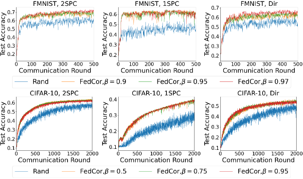
Refer to caption
Figure 8: Test accuracy with different annealing coefficient β𝛽\beta on FMNIST (top) and CIFAR-10 (bottom) under three heterogeneous settings (left: 2SPC; median: 1SPC; right: Dir).

C.2 Dirichlet Distribution for Data Partition

We follow the idea in [7] to construct the Dir heterogeneous setting, while we make some modifications to get an unbalanced non-identical data distribution.

For each client k𝑘k, we sample the data distribution 𝒒k10subscript𝒒𝑘superscript10\bm{q}_{k}\in\mathbb{R}^{10} from a dirichlet distribution independently, which could be formulated as

𝒒kDir(α𝒑),similar-tosubscript𝒒𝑘Dir𝛼𝒑\bm{q}_{k}\sim\text{Dir}(\alpha\bm{p}), (146)

where 𝒑𝒑\bm{p} is the prior label distribution and α+𝛼subscript\alpha\in\mathbb{R}_{+} is the concentration parameter of the dirichlet distribution. We group 𝒒ksubscript𝒒𝑘\bm{q}_{k} of all the clients together and get a fraction matrix Q=[𝒒1,,𝒒n]𝑄subscript𝒒1subscript𝒒𝑛Q=[\bm{q}_{1},\cdots,\bm{q}_{n}]. We denote the size of dataset on each client as 𝒙=[x1,,xN]T𝒙superscriptsubscript𝑥1subscript𝑥𝑁𝑇\bm{x}=[x_{1},\cdots,x_{N}]^{T} and we get it from a solution of a quadratic programming:

min𝒙subscript𝒙\displaystyle\min_{\bm{x}}\quad 𝒙T𝒙superscript𝒙𝑇𝒙\displaystyle\bm{x}^{T}\bm{x} (147)
subject to Q𝒙=𝒅𝑄𝒙𝒅\displaystyle Q\bm{x}=\bm{d} (148)
𝒙++N,𝒙superscriptsubscriptabsent𝑁\displaystyle\bm{x}\in\mathbb{R}_{++}^{N}, (149)

where 𝒅𝒅\bm{d} is the number of data with each label. We minimize 𝒙2subscriptnorm𝒙2\|\bm{x}\|_{2} to avoid the cases where data distribution is over-concentrated on a small fraction of clients. In that case, the client selection problem might become trivial, since we can always ignore those clients with a small dataset and select those with a large dataset.

Appendix D Extra Experimental Results

D.1 Ablation Study: Annealing Coefficient

We conduct experiments on FMNIST and CIFAR-10 with different annealing coefficient β𝛽\beta. We setup our experiments under three heterogeneous settings as in Section 5, with different annealing coefficient β𝛽\beta (β=0.95,0.75,0.5𝛽0.950.750.5\beta=0.95,0.75,0.5 for FMNIST and β=0.97,0.95,0.9𝛽0.970.950.9\beta=0.97,0.95,0.9 for CIFAR-10). We fix the GP training interval ΔtΔ𝑡\Delta t to 101010 for FMNIST and 505050 for CIFAR-10. The test accuracy curves are shown in Figure 8. We can see that within a large range, the value of annealing coefficient only slightly influence the convergence rate as well as the final accuracy. Recalling the results of different GP training intervals ΔtΔ𝑡\Delta t in Section 5.3, we can say that our method is not sensitive to the hyperparameters ΔtΔ𝑡\Delta t and β𝛽\beta.

We present the selected frequency of each client in Figure 10 and Figure 11 for FMNIST and CIFAR-10 respectively. We can see that with a smaller β𝛽\beta, the selected frequency tends to be more “uniform”. However, this does not mean that our selection strategy is equivalent to the uniformly random selection. Our sequential selection strategy introduces dependencies between selected clients as discussed in the multi-iteration insights in Section 4.3, which makes our selection strategy prefer some combinations of selected clients to others, while the uniformly random selection treats all the combinations equally. The advantage shown in Figure 8 compared to the uniformly random strategy demonstrates that selecting a good combination of clients, not only a good individual, is important.
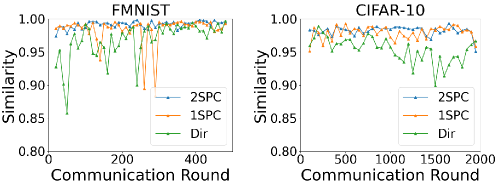
Refer to caption
Figure 9: Verification of covariance stationarity on FMNIST and CIFAR-10.

D.2 Normality Verification

We setup experiments to show that Gaussian Distribution can model the loss changes w.r.t. uniformly sampled client selection. To verify this, in the last round of the warm-up phase, we perform the following procedure to examine the normality.

  1. 1.

    We uniformly sample 100010001000 different client selections {𝕊t,i:i=1,,1000}conditional-setsubscript𝕊𝑡𝑖𝑖11000\{{\mathbb{S}}_{t,i}:i=1,\cdots,1000\} and collect the corresponding loss changes Δ𝒍t(𝕊t,i)=[Δl1t(𝕊t,i),,ΔlNt(𝕊t,i)]Δsuperscript𝒍𝑡subscript𝕊𝑡𝑖Δsuperscriptsubscript𝑙1𝑡subscript𝕊𝑡𝑖Δsuperscriptsubscript𝑙𝑁𝑡subscript𝕊𝑡𝑖\Delta{\bm{l}}^{t}({\mathbb{S}}_{t,i})=[\Delta l_{1}^{t}({\mathbb{S}}_{t,i}),\cdots,\Delta l_{N}^{t}({\mathbb{S}}_{t,i})] for each of them.

  2. 2.

    We perform PCA on {Δ𝒍t(𝕊t,i):i=1,,1000}conditional-setΔsuperscript𝒍𝑡subscript𝕊𝑡𝑖𝑖11000\{\Delta{\bm{l}}^{t}({\mathbb{S}}_{t,i}):i=1,\cdots,1000\} to extract the principle components.

  3. 3.

    We plot the histogram of each principle component and compare its distribution with the Gaussian Distribution.

We do not use Multivariate Normality Test directly because we find that 𝚺𝒕superscript𝚺𝒕\bm{\Sigma^{t}} is always nearly singular, which makes the Multivariate Normality Test unstable. Thus, we turn to perform PCA and visualize each principle component to verify the normality.

The results of FMNIST and CIFAR-10 are shown in Figure 12 and Figure 13 respectively. The red line shows the probability density of Gaussian Distribution with the mean and variance of that principle component. We can see that in all our experiments, Gaussian Distribution can fit the distribution of the principle component well, which verifies that Lemma 1 does hold in all the experiment settings.

D.3 Covariance Stationarity Verification

We examine that assumption in Section 4.5 that the covariance keep approximately stationary during the FL training, namely,

t,𝚺t𝚺t+Δt.for-all𝑡superscript𝚺𝑡superscript𝚺𝑡Δ𝑡\forall t,{\bm{\Sigma}}^{t}\approx{\bm{\Sigma}}^{t+\Delta t}. (150)

To verify this, every ΔtΔ𝑡\Delta t rounds (Δt=10Δ𝑡10\Delta t=10 for FMNIST and Δt=50Δ𝑡50\Delta t=50 for CIFAR-10), we randomly sample 100010001000 client selections 𝕂isubscript𝕂𝑖{\mathbb{K}}_{i} and collect the corresponding loss changes Δ𝒍t(𝕂i)Δsuperscript𝒍𝑡subscript𝕂𝑖\Delta{\bm{l}}^{t}({\mathbb{K}}_{i}). We directly calculate the covariance matrix 𝚺tsuperscript𝚺𝑡{\bm{\Sigma}}^{t} with these samples {Δ𝒍t(𝕂i):i=1,,1000}conditional-setΔsuperscript𝒍𝑡subscript𝕂𝑖𝑖11000\{\Delta{\bm{l}}^{t}({\mathbb{K}}_{i}):i=1,\cdots,1000\}. Then for each adjacent pair of covariance matrix, we calculate their cosine similarity as follows.

similarity(𝚺t,𝚺t+Δt)=tr(𝚺tT𝚺t+Δt)tr(𝚺tT𝚺t)tr(𝚺t+ΔtT𝚺t+Δt)similaritysuperscript𝚺tsuperscript𝚺tΔttrsuperscriptsuperscript𝚺tTsuperscript𝚺tΔttrsuperscriptsuperscript𝚺tTsuperscript𝚺ttrsuperscriptsuperscript𝚺tΔtTsuperscript𝚺tΔt\rm{similarity}({\bm{\Sigma}}^{t},{\bm{\Sigma}}^{t+\Delta t})=\frac{\rm{tr}({{\bm{\Sigma}}^{t}}^{T}{\bm{\Sigma}}^{t+\Delta t})}{\rm{tr}({{\bm{\Sigma}}^{t}}^{T}{\bm{\Sigma}}^{t})\rm{tr}({{\bm{\Sigma}}^{t+\Delta t}}^{T}{\bm{\Sigma}}^{t+\Delta t})} (151)

The similarity is in range [0,1]01[0,1], and a larger one shows a higher similarity.

The results are shown in Figure 9. We can see that in most cases the similarity is larger than 0.90.90.9, which verifies our claim of the covariance stationarity.
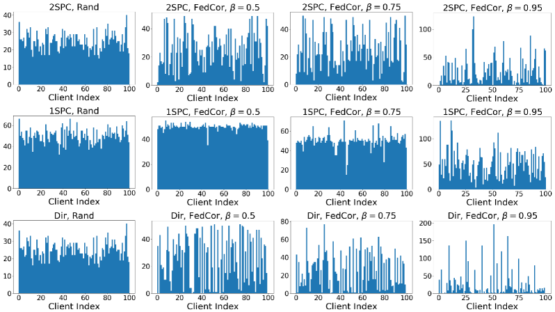
Refer to caption
Figure 10: Selected Frequency of each client with different annealing coefficient β𝛽\beta on FMNIST under three heterogeneous settings (top: 2SPC; median: 1SPC; bottom: Dir).
Refer to caption
Figure 11: Selected Frequency of each client with different annealing coefficient β𝛽\beta on CIFAR-10 under three heterogeneous settings (top: 2SPC; median: 1SPC; bottom: Dir).
Refer to caption
Figure 12: Normality Test on FMNIST.
Refer to caption
Figure 13: Normality Test on CIFAR-10.