Computationally-Efficient Roadmap-based Inspection Planning via Incremental Lazy Search

Abstract

The inspection-planning problem calls for computing motions for a robot that allow it to inspect a set of points of interest (POIs) while considering plan quality (e.g., plan length). This problem has applications across many domains where robots can help with inspection, including infrastructure maintenance, construction, and surgery. Incremental Random Inspection-roadmap Search (IRIS) is an asymptotically-optimal inspection planner that was shown to compute higher-quality inspection plans orders of magnitudes faster than the prior state-of-the-art method. In this paper, we significantly accelerate the performance of IRIS to broaden its applicability to more challenging real-world applications. A key computational challenge that IRIS faces is effectively searching roadmaps for inspection plans—a procedure that dominates its running time. In this work, we show how to incorporate lazy edge-evaluation techniques into IRIS’s search algorithm and how to reuse search efforts when a roadmap undergoes local changes. These enhancements, which do not compromise IRIS’s asymptotic optimality, enable us to compute inspection plans much faster than the original IRIS. We apply IRIS with the enhancements to simulated bridge inspection and surgical inspection tasks and show that our new algorithm for some scenarios can compute similar-quality inspection plans $570\times$ faster than prior work.

I Introduction

We consider the problem of inspection planning where a robot needs to inspect a set of points of interest (POIs) in a given environment with its on-board sensor while optimizing plan cost. This problem has numerous applications such as product surface inspections for industrial quality control [1], structural inspections with unmanned aerial vehicles (UAVs) [2, 3, 4, 5, 6], ship-hull inspections [7, 8, 9], underwater inspections for scientific surveying [10, 11, 12, 13], and patient-anatomy inspections in medical-endoscopic procedures for disease diagnosis [14].

Roughly speaking, the inspection-planning problem is computationally challenging because we need to simultaneously reason both about plan cost and about inspecting the POIs. Unfortunately, even computing a minimal-cost plan (without reasoning about inspection) is already PSPACE-hard in the general case [15]. The problem is exasperated in our setting as the search space over motion plans grows exponentially with the number of POIs to inspect [16]. Thus, the cost of naïvely-computed inspection plans may be orders of magnitude higher than the cost of an optimal plan, and computing a high-quality plan (especially with bounds on the solution quality) may be extremely time-consuming. For time-sensitive applications, generating a high-quality inspection plan in a short computation time (i.e., the time between starting to solve an instance of the problem and getting a result) is critical. For example, for patient anatomy inspection planned according to pre-operative medical images (Fig. 1 top right), a short computation time reduces overall procedure time and makes faster diagnosis possible, which has the potential to improve patient outcomes. Even for non-time-sensitive applications (e.g., bridge inspection as shown in Fig. 1 top left), better computing efficiency means, with the same computing power, we can achieve similar-quality results faster or achieve better-quality results given the same computation time.

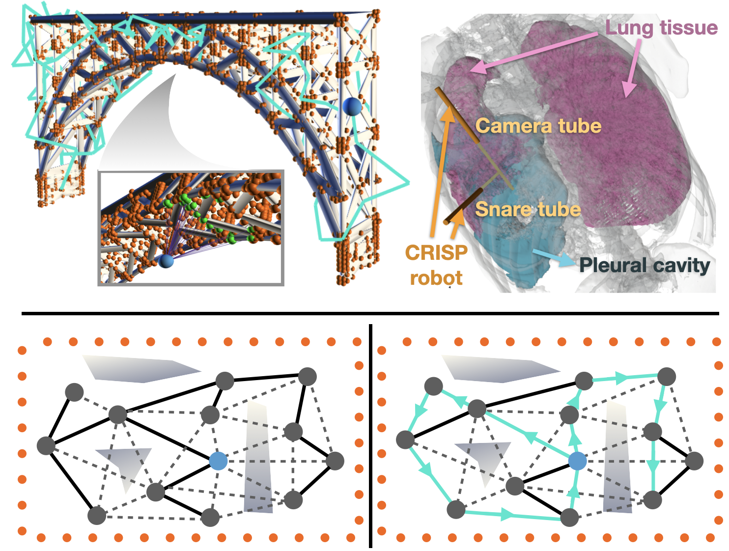
Figure 1: Top: Example applications of inspection planning. Top left: An unmanned aerial vehicle (blue sphere) inspecting a bridge with its on-board sensor (e.g., camera) by following the inspection plan (aquamarine). Points of interest (POIs) are shown as orange spheres (visible POIs are green in zoomed-in part). A POI is considered inspected if it is visible to the sensor. Top right: The Continuum Reconfigurable Incisionless Surgical Parallel (CRISP) robot [17, 18], a medical robot composed of flexible needle-diameter tubes and equipped with a camera, can perform endoscopic diagnosis in the pleural cavity (the space between the lung surface and chest wall) for a patient with excess fluid surrounding the lung. The inspection enables a physician to diagnose underlying disease. Bottom: IRIS [16] computes a collision-free plan (aquamarine) to inspect POIs (orange dots). It searches a roadmap (dashed edges) implicitly defined by a tree structure (vertices and solid edges) embedded in the configuration space rooted at the start configuration (blue vertex). As the roadmap is densified, the resulting inspection plan asymptotically converges to a global optimum.

To enable faster computation of high-quality inspection plans, we propose algorithmic enhancements to accelerate the performance of Incremental Random Inspection-roadmap Search (IRIS) [16]. IRIS constructs an incrementally-densified roadmap, a graph representing robot states and transitions between the states. Then IRIS searches over the roadmap for a near-optimal inspection plan. In this paper, we accelerate IRIS’s performance while retaining its formal guarantee of asymptotic optimality.

We accelerate IRIS’s performance in two significant ways. First, we need to build roadmaps that are compact and yet informative for inspection planning. In this paper, we present a simple-yet-effective solution where we reduce the number of samples that fail to inspect previously-uncovered POIs (i.e., POIs not seen by the robot’s sensor from any prior robot state on the roadmap) with coverage-informed sampling during roadmap construction. Second, we observe that graph search dominates computation time when the graph grows larger, motivating the need for a fast method to effectively search the gradually-densified roadmap. The original IRIS runs every search iteration from scratch, disregarding that the roadmap is incrementally densified, but search efforts from previous iterations are potentially helpful in later iterations. So in this paper, we show (i) how to incorporate refined lazy edge-evaluation techniques [19] into IRIS and (ii) how to reuse search efforts when a roadmap locally changes.

These enhancements, which do not compromise IRIS’s asymptotic optimality, enable us to compute inspection plans much faster than the original IRIS. We evaluate our algorithm in simulation in bridge inspection and surgical inspection scenarios. Experimental results show that IRIS with the enhancements for some scenarios can compute inspection plans of similar-quality $570\times$ faster than the original IRIS.

II Related Work

Inspection planning typically calls for solving two subtasks: (i) viewpoints planning that determines a set of viewpoints collectively covering all POIs and (ii) trajectory planning that determines a trajectory connecting the viewpoints. Many methods solve these subtasks separately. For viewpoints planning, early methods compute a minimal set of viewpoints by solving the Art Gallery Problem [20]. However, a minimal set of viewpoints doesn’t guarantee the optimality of the final plan [21]. So later methods find only a set of viewpoints that satisfies the inspection requirements. Then the trajectory-planning task is usually formulated using variants of the Traveling Salesman Problem (TSP) [22, 23, 24, 25]. To improve the quality of the solution, some use trajectory optimization [26, 27] while others resample viewpoints [3, 4], or adaptively sample viewpoints [6]. Unfortunately, this decomposition into two separate steps forgoes any guarantees on the quality of the solution.

Most existing methods for inspection planning (as mentioned above) do not provide formal guarantees on the quality of final solutions. But recent approaches [16, 21, 28, 29] provide asymptotic guarantees by making use of advances in sampling-based motion planners [30]. Specifically, these methods are based on asymptotically-optimal motion planners [31] such as the probabilistic roadmap* (PRM*), the rapidly-exploring random tree* (RRT*), and the rapidly-exploring random graph (RRG) [32]. Roughly speaking, these methods guarantee that as the number of samples used by the algorithm approaches infinity, the cost of the solution obtained converges to the optimal cost. Such an asymptotic-optimality guarantee comes at a price of long computation time. Notable among the inspection planners that do provide formal guarantees on the quality of the solution, IRIS was shown to compute higher-quality inspection plans orders of magnitudes faster [16] than the prior state-of-the-art method, Rapidly-exploring Random Tree of Trees (RRTOT) [28].

For additional related work discussing the connection of inspection planning to other fields, please refer to [33, 34].

III Problem Definition

The robot operates in some physical workspace $\mathcal{W}\subset\mathbb{R}^{d}$ where $d\in\{2,3\}$. The workspace is cluttered with obstacles $\mathcal{W}_{\rm obs}\subset\mathcal{W}$. A robot’s configuration $\mathbf{q}$ is a vector of parameters that uniquely defines its state (e.g., joint angles for a manipulator arm, pose for an aerial vehicle), and the set of all configurations $\mathcal{C}$ is defined as its configuration space or C-space. Given a configuration $\mathbf{q}$, we can compute the subset of the workspace $\mathcal{W}$ occupied by the robot ${\rm Occupancy}(\mathbf{q})\subset\mathcal{W}$. We say that $\mathbf{q}$ is collision free if ${\rm Occupancy}(\mathbf{q})\cap\mathcal{W}_{\rm obs}=\emptyset$ and in-collision otherwise. This subdivides the C-space $\mathcal{C}$ into the free space $\mathcal{C}_{\rm free}\subset\mathcal{C}$ and obstacle space $\mathcal{C}_{\rm obs}=\mathcal{C}\setminus\mathcal{C}_{\rm free}$. A robot’s path is a mapping $\pi:[0,1]\rightarrow\mathcal{C}$. It is valid if it follows the kinematic constraints of the robot and if $\forall t\in[0,1],\pi(t)$ is collision free. In this work we will discretize the path into a finite sequence of configurations $\{\pi(t_{0}),\ldots,\pi(t_{k})\}$ with $k\geq 0$, $t_{i}<t_{i+1}$, and $t_{i}\in[0,1]$. We use linear interpolation between configurations for collision checking. We are given some cost function ${\rm Cost}:\mathcal{C}\times\mathcal{C}\rightarrow\mathbb{R}$ and we extend it to paths ${\rm Cost}(\pi)=\sum_{i=0}^{k-1}{\rm Cost}(\pi(t_{i}),\pi(t_{i+1}))$. Our framework can deal with general cost functions, but in this particular work, we use path length $\ell(\cdot)$ as cost.

We are given a discrete set $\mathcal{I}=\{i_{0},...,i_{N}\}\subset\mathcal{W}$ of points of interest (POIs) that we need to inspect given some sensor mounted on the robot. The sensor is modeled by the mapping $\mathcal{S}:\mathcal{C}\rightarrow 2^{\mathcal{I}}$ (where $2^{\mathcal{I}}$ is the powerset of $\mathcal{I}$) that states which POIs can be seen from a given configuration. A configuration will also be referred to as a viewpoint. We will say that a POI $i\in\mathcal{I}$ is covered by a configuration $\mathbf{q}$ (or that $\mathbf{q}$ covers $i$) if $i\in\mathcal{S}(\mathbf{q})$. By a slight abuse of notation, we extend the sensor model to paths and have that $\mathcal{S}(\pi)=\bigcup_{i=0}^{k}\mathcal{S}(\pi(t_{i}))$ is the inspection coverage of a path $\pi$.

Given a C-space $\mathcal{C}$, a start configuration $\mathbf{q}_{\rm s}\in\mathcal{C}_{\rm free}$, a set of POIs $\mathcal{I}$, a sensor model $\mathcal{S}$, and a cost function ${\rm Cost}$, the optimal inspection plan is a valid path $\pi^{*}={\rm argmin}_{\pi\in\Pi}{\rm Cost}(\pi)$. Here, $\Pi$ is the set of paths maximizing the inspection coverage, more formally, $\Pi=\{\pi|\pi={\rm argmax}_{\pi\in\Pi_{\mathbf{q}_{s}}}|\mathcal{S}(\pi)|\}$, where $|\cdot|$ is the cardinality and $\Pi_{\mathbf{q}_{s}}$ is the set of paths starting from $\mathbf{q}_{\rm s}$.

IV Algorithmic Background

IV-A Incremental Random Inspection-roadmap Search (IRIS)

IRIS incrementally constructs a sequence of increasingly-dense graphs, or roadmaps, embedded in the C-space and computes an inspection plan over the roadmaps as they are constructed [16]. To build the roadmap, IRIS builds an RRG. However, since not all the edges will be used and edge evaluation can be computationally expensive, IRIS takes a lazy edge-evaluation approach. This is done by explicitly constructing an RRT [30] (which is a subgraph of an RRG when constructed using the same set of vertices) and leaving all other edges un-evaluated that implicitly define the RRG. The rest of the edges are evaluated on demand during the graph search (for more details see Sec. V).

Computing an optimal-inspection plan on a roadmap $\mathcal{G}=(\mathcal{V},\mathcal{E})$ with $n$ vertices is computationally hard because we need to compute the shortest path on a so-called inspection graph. Here, each vertex corresponds to a vertex $v\in\mathcal{V}$ of the original graph $\mathcal{G}$ and a subset $I$ of $\mathcal{I}$, representing a path ending at $v$ while inspecting $I$. Thus, the inspection graph has $O(n\times|2^{\mathcal{I}}|)$ vertices. To search this inspection graph, IRIS employs a novel search algorithm that approximates $\pi^{*}$, the optimal inspection path on the graph. To this end, IRIS uses two parameters, $\varepsilon$ and $p$, to ensure that the path obtained from the graph-search phase is no longer than $1+\varepsilon$ the length of $\pi^{*}$ and covers at least $p$ percent of the POIs covered by $\pi^{*}$. To ensure convergence to the optimal inspection path, $\varepsilon$ is reduced and $p$ is increased between search iterations. This is referred to as tightening the approximation factors.

We now briefly describe the graph-search algorithm as it is key to understanding the algorithmic contributions of this work. For an in-depth description of the search algorithm, the rest of the framework, and its theoretical guarantees, see [16]. The search runs an A*-like search [35] but instead of having each node represent a path from the start vertex $\mathbf{q}_{s}$, each node is a path pair PP that is composed of a so-called achievable path (AP) and potentially achievable path (PAP). As its name suggests, an AP represents a path in the graph from $\mathbf{q}_{s}$. In contrast, a PAP is not necessarily realizable and is used to bound the quality of paths represented by a specific PP. A $\textsf{PP}=(P,\tilde{P})$, where $P$ is the AP and $\tilde{P}$ is the PAP, is said to be $\varepsilon,p$-bounded if (i) $\ell(P)\leq(1+\varepsilon)\ell(\tilde{P})$ and (ii) $|\mathcal{S}(P)|\geq p\cdot|\mathcal{S}(\tilde{P})|$.

Similar to A*, the algorithm uses an OPEN and CLOSED list to track nodes that have not and have been considered, respectively. It starts with the trivial path pair, $\textsf{PP}_{\mathbf{q}_{s}}$, where both AP and PAP represent the trivial path $\{\mathbf{q}_{s}\}$.

At each iteration, it pops a node from the OPEN list, and checks if the search can terminate. If not, the node is extended and added to the CLOSED list. While doing so, the algorithm tests if successor nodes can subsume or be subsumed by another node. These two core operations (extending and subsuming) are key to the efficiency of the algorithm and we now elaborate on them for a given path pair $\textsf{PP}_{u}=(P_{u},\tilde{P_{u}})$ (here $P_{u}$ is AP and $\tilde{P_{u}}$ is PAP):

1. Extending operation: Extending $\textsf{PP}_{u}$ by edge $e=(u,v)\in\mathcal{E}$ (denoted $\textsf{PP}_{u}+e$) will extend both $P_{u}$ and $\tilde{P_{u}}$ by edge $e$. The resulting path pair is $\textsf{PP}_{v}=(P_{v},\tilde{P_{v}})$, where the AP satisfies $\mathcal{S}(P_{v})=\mathcal{S}(P_{u})\cup\mathcal{S}(v),\ell(P_{v})=\ell(P_{u})+\ell(e)$, and the PAP satisfies $\mathcal{S}(\tilde{P_{v}})=\mathcal{S}(\tilde{P_{u}})\cup\mathcal{S}(v),\ell(\tilde{P_{v}})=\ell(\tilde{P_{u}})+\ell(e)$.

2. Subsuming operation: Given two path pairs $\textsf{PP}_{1}=(P_{1},\tilde{P_{1}})$ and $\textsf{PP}_{2}=(P_{2},\tilde{P_{2}})$ that end at the same vertex, the operation of $\textsf{PP}_{1}$ subsuming $\textsf{PP}_{2}$ (denoted $\textsf{PP}_{1}\oplus\textsf{PP}_{2}$) will create a new path pair $\textsf{PP}_{1}\oplus\textsf{PP}_{2}:=\left(P_{1},\left(\mathcal{S}(\tilde{P_{1}})\cup\mathcal{S}(\tilde{P_{2}}),\min(\ell(\tilde{P_{1}}),\ell(\tilde{P_{2}}))\right)\right)$.

Roughly speaking, the subsuming operation allows to reduce the number of paths considered by the search. However, to ensure that the solution returned by the algorithm approximates the optimal inspection path, subsuming only occurs when the resultant PP is $\varepsilon,p$-bounded.

IV-B IRIS limitations

IRIS was shown to dramatically outperform the prior state-of-the-art in asymptotically-optimal inspection planning [16]. However, a close analysis of the algorithm’s building blocks allows us to pinpoint the computational challenges faced by IRIS which, in turn, will allow us to suggest new algorithmic enhancements.

1. Configuration sampling in roadmap generation. To generate a roadmap, IRIS randomly samples configurations in the C-space. Thus, the coverage of a newly-sampled configuration is not accounted for when generating the roadmap. This has the potential to increase the roadmap size without adding new (or adding very little) POIs which, in turn, will induce long search times.

2. Edge evaluation during graph search. As mentioned in [16], the edge-evaluation scheme employed by IRIS assumes that edge-evaluation dominates the algorithm’s running time. This is true when the size of the roadmap is small but as the number of vertices grows, search dominates the algorithm’s running time.

3. Iterative graph search. IRIS runs a new graph search after adding configurations to the roadmap. In the original formulation, the search tree obtained from previous search episodes is discarded and the search algorithm is run from scratch. This can be highly inefficient as often the new graph is very similar to the one used in the previous iterations.

V Method

We propose several enhancements to IRIS corresponding to the algorithmic challenges detailed in Sec. IV-B.

V-A Coverage-informed sampling

To improve the computational efficiency of the original IRIS, we propose to replace uniform sampling of configurations (used to construct the roadmap) with an approach that we call coverage-informed sampling that accounts for the inspection coverage of sampled configurations. Our approach, which bears resemblance to advanced sampling schemes used in motion planning (see, e.g., [36, 37]), works as follows: given a randomly-sampled configuration $\mathbf{q}_{\rm rand}$, we accept it directly with some probability $p_{\rm{accept}}>0$. If the configuration was not directly accepted, we test if $|\mathcal{S}(\mathcal{V})\cup\mathcal{S}(\mathbf{q_{\rm rand}})|>|\mathcal{S}(\mathcal{V})|,$ where $\mathcal{S}(\mathcal{V})$ is the set of POIs collectively covered by roadmap vertices. If the test passes (namely, if $\mathbf{q_{\rm rand}}$ covers previously-uncovered POIs), we accept $\mathbf{q_{\rm rand}}$ and add it to the roadmap. If not, the configuration is rejected.

Randomly accepting $\mathbf{q_{\rm rand}}$ is important for maintaining the theoretical guarantees of IRIS (i.e., asymptotic convergence to the optimal inspection path), since $\mathbf{q_{\text{rand}}}$ can be used to reduce path length regardless of its coverage. This is similar to the way goal-biasing is employed in sampling-based motion planners [38].

In addition, as graph search dominates the algorithm’s running time, we would typically like to initiate a search only when roadmap coverage increases significantly. Thus, we define a relaxation parameter $\omega\in(0,1]$ and run a new search only when $|\mathcal{S}(\pi_{\rm prev})|<\omega\cdot p\cdot|\mathcal{S}(\mathcal{V})|$. Here, $\pi_{\rm prev}$ is the path returned by the previous search iteration. This can be seen as a generalization of the original IRIS which uses $\omega=1.0$. As with the original IRIS, after $N_{\max}$ new vertices were sampled without a new search being initiated, we run a new search regardless of the additional coverage. This allows us to keep reducing the plan’s length even when the coverage does not increase (or increases slowly). In all our experiments, we use $\omega=0.9$ and $N_{\max}=200$.

V-B Refined lazy edge evaluation

Similar to many motion-planning algorithms, the original IRIS takes a lazy edge-evaluation approach [39, 40, 41, 42, 43] during graph search. Specifically, it uses the LazySP framework [42] where all edges are assumed to be collision-free and the search is run until a path is found. Edges along this path are then evaluated one-by-one. If we find an in-collision edge, we discard it and rerun the search. If all edges are collision-free then the path is returned. While this approach was shown to minimize the number of edges evaluated [44], the computational price of having multiple search episodes can increase overall running times in motion planning algorithms [45, 46].

An alternative lazy search algorithm is LazyA* which was shown to minimize search efforts [19]. Here, edges are assumed to be collision-free until a node is expanded and only then its incoming edge is evaluated (for additional details, see [19]). Unfortunately, we cannot use a LazyA*-like approach as-is because of the way paths are subsumed in the near-optimal search algorithm. Specifically, in our setting, when a node (PP) is to be extended, it may have already subsumed other nodes (PPs). If we discard such a node because its incoming edge is in-collision (as would have been done in LazyA*) then we discard all the information about the subsumed nodes, including potentially-valid ones. This subtlety requires us to additionally validate a node’s incoming edges when it is to subsume other nodes.

To this end, we consider two types of nodes (PPs)—trivial (T) and non-trivial (NT) which correspond to PPs that did not and did subsume another PP, respectively. Note that by our definition a T-node may be a descendent of an NT-node. We validate the incoming edge of a T-node when either (i) it is extracted from the OPEN list (similar to LazyA*) or when (ii) it is to subsume another node (thus becoming an NT-node which implies that all incoming edges of NT-nodes are validated). For a visualization, see Fig. 2.

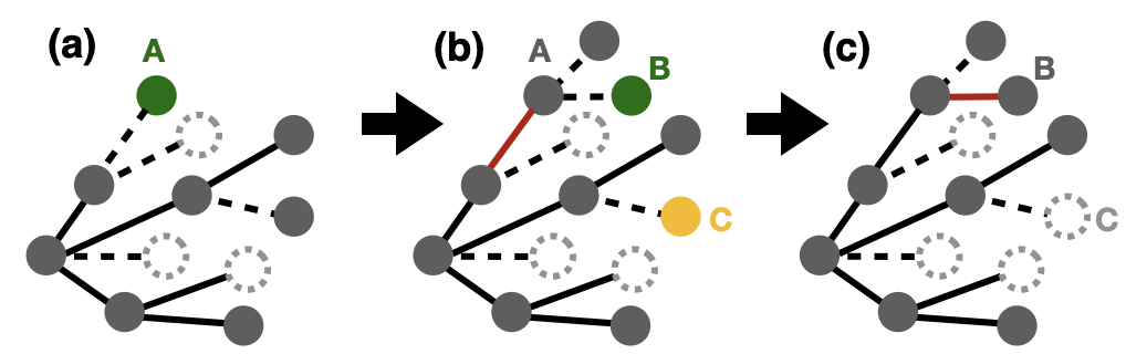
Figure 2: Two different edge evaluation cases. Each node in the search tree is a PP, and nodes with dashed boundaries have been subsumed. Solid and dashed lines are validated and yet-to-be validated incoming edges, respectively. Red edges are the edges being validated in the current step. First case: validating incoming edge of a T-node ((a) to (b)). When extending a T-node A, we validate its incoming edge. Second case: validating incoming edge when a T-node is to subsume another node ((b) to (c)). When a T-node B is to subsume another node C, we validate its incoming edge.

V-C Incremental search by reusing efforts across iterations

In the original IRIS, every new search is run from scratch and the only information shared between search iterations is edge validity. Fortunately, reusing search information across different search iterations is a well-studied problem [47, 48, 49] that has been successfully used in many motion-planning algorithms (see, e.g., [40, 43, 45, 50, 51]).

In typical approaches, between two search episodes, all nodes and data structures (e.g., OPEN and CLOSED lists in A*) are stored. After an edge or vertex is added or removed from the graph, we first identify all inconsistent nodes (namely, whose cost changed due to the change in the graph), then their cost is updated and they are re-added to the relevant data structures. Unfortunately, we cannot use these methods as-is because of the way the approximation factor changes between search iterations.

The crux of the problem is that even if there is no change in the graph, tightening the approximation factors $\varepsilon$ and $p$ may cause nodes (i.e., path pairs) in the search tree to no longer be $\varepsilon,p$-bounded (for the new values of $\varepsilon$ and $p$). To this end, we first discuss how we ensure that before executing a new search, all nodes in the search tree (namely, in the OPEN and CLOSED lists) are $\varepsilon,p$-bounded when there are no changes to the graph. We then describe how to account for the additional vertices and edges added to $\mathcal{G}$.

V-C1 Accounting for tightening of the approximation factors

Recall that in our search algorithm, we have two basic operations on nodes: extending the associated path pair PP by an edge and subsuming another path pair. The former can only decrease the (relative) gap between the achievable path (AP) and the potentially achievable path (PAP) of the PP. In contrast, the latter may increase the (relative) gap between the AP and PAP of the PP. Thus, after tightening the approximation factors $\varepsilon$ and $p$, nodes that are still $\varepsilon,p$-bounded may have unbounded predecessors.

If a node is no longer $\varepsilon,p$-bounded, we need to “rollback“ previous subsuming operations to obtain nodes that are $\varepsilon,p$-bounded. This requires us to store for each PP not only the AP and PAP but also a list of all PPs that were subsumed and may dramatically increase the program’s memory footprint. To reduce unnecessary memory usage, we perform the following optimization: when the subsuming operation $\textsf{PP}_{1}\oplus\textsf{PP}_{2}$ is performed, if $\mathcal{S}(P_{1})\supseteq\mathcal{S}(\tilde{P_{2}}),\ell(P_{1})\leq\ell(\tilde{P_{2}})$, then $\textsf{PP}_{2}$ is not stored in the subsumed list. This is because the PAP of $\textsf{PP}_{2}$ (which is a lower bound on the solution that can be obtained using that node) is strictly dominated by the AP of $\textsf{PP}_{1}$ (which, by definition, can be obtained). To further reduce memory usage, instead of storing $\textsf{PP}_{2}$ directly, we store the predecessor of $\textsf{PP}_{2}$. Since the ending vertex of $\textsf{PP}_{2}$ is the same as $\textsf{PP}_{1}$ thus is known, we can easily reconstruct $\textsf{PP}_{2}$ from its predecessor if need to. Since $\textsf{PP}_{2}$ is not directly stored, the nodes subsumed by $\textsf{PP}_{2}$ (if any) are inherited by $\textsf{PP}_{1}$ when $\textsf{PP}_{1}$ subsumes $\textsf{PP}_{2}$.

To reuse search efforts, we define two characteristics of nodes. First, a node is revealed (if stored in the OPEN or CLOSED list) or hidden (if subsumed and stored in the subsumed list of another node). And a node can be a reusable, boundary, or non-reusable node (see also, Fig. 3):

1. Reusable nodes—a node is reusable if it is $\varepsilon,p$-bounded and all its predecessors are also $\varepsilon,p$-bounded.

2. Boundary nodes—a node is a boundary node if it is no longer $\varepsilon,p$-bounded, but all its predecessors are.

3. Non-reusable nodes—a node is non-reusable if it has at least one predecessor that is no longer $\varepsilon,p$-bounded.

As the name suggests, reusable nodes can be used as-is. Thus, we keep revealed reusable nodes in the OPEN or CLOSED list, depending on where they were when the previous search terminated.

Before we discuss how we handle boundary and non-reusable nodes, notice that given a boundary node $\textsf{PP}_{v}$ with parent $\textsf{PP}_{u}$, we have that extending $\textsf{PP}_{u}$ by the edge $(u,v)$ (denoted as $\textsf{PP}_{u}+(u,v)$) yields a new path pair $\hat{\textsf{PP}}_{v}$ to $v$ that is $\varepsilon,p$-bounded (with an empty list of subsumed nodes). Thus, we start by adding all revealed boundary and non-reusable nodes into a list which we call RELEASE and removing them from the OPEN or CLOSED list. Nodes from RELEASE are popped one by one until it is empty. For each node, $\textsf{PP}_{v}$, popped from RELEASE we (i) add $\textsf{PP}_{v}$ (if it is a reusable node) or $\textsf{PP}_{u}+(u,v)$ (if it is a boundary node) to the OPEN list (while testing for dominance as in the original IRIS), and (ii) add all of $\textsf{PP}_{v}$’s subsumed nodes to RELEASE in case it is a boundary or a non-reusable node.

While a complete proof of the correctness of our approach is beyond the scope of this paper, we notice that: (i) after the above operations, all revealed nodes (either in the OPEN or CLOSED list) are $\varepsilon,p$-bounded; (ii) for every node $\textsf{PP}_{v}$ (either revealed or hidden) from the previous search iteration, if $\textsf{PP}_{v}$ is not in the CLOSED list, then either $\textsf{PP}_{v}$ or one of its predecessors is either in the OPEN list or in the subsumed list of a node in the OPEN or CLOSED list, which means that all nodes are accounted for. The above properties guarantee that the new search still results in a near-optimal solution.

V-C2 Accounting for roadmap updates

To further account for new vertices and edges, for any node $\textsf{PP}_{u}$ in the CLOSED list corresponding to a vertex $u\in\mathcal{V}$ that has an edge $(u,v)$ to a newly-inserted vertex $v$, we add the new successor $\textsf{PP}_{u}+(u,v)$ to the OPEN list.

V-C3 Putting it all together

To summarize, our new search algorithm receives as input not only $\mathcal{G}$, $\mathbf{q}_{s}$, $\varepsilon$ and $p$, but also the OPEN and CLOSED lists from the previous search iteration (if it is the first iteration then both are empty). We start by adding the node used to obtain the path in the previous iteration back into the OPEN list (if it is the first iteration, we add $\textsf{PP}_{\mathbf{q}_{s}}$). We then continue to update the OPEN and CLOSED lists to account for the tightening of the approximation factors (Sec. V-C1) and then we update the OPEN list to account for the roadmap updates (Sec. V-C2). Finally, we run our search algorithm without any changes.

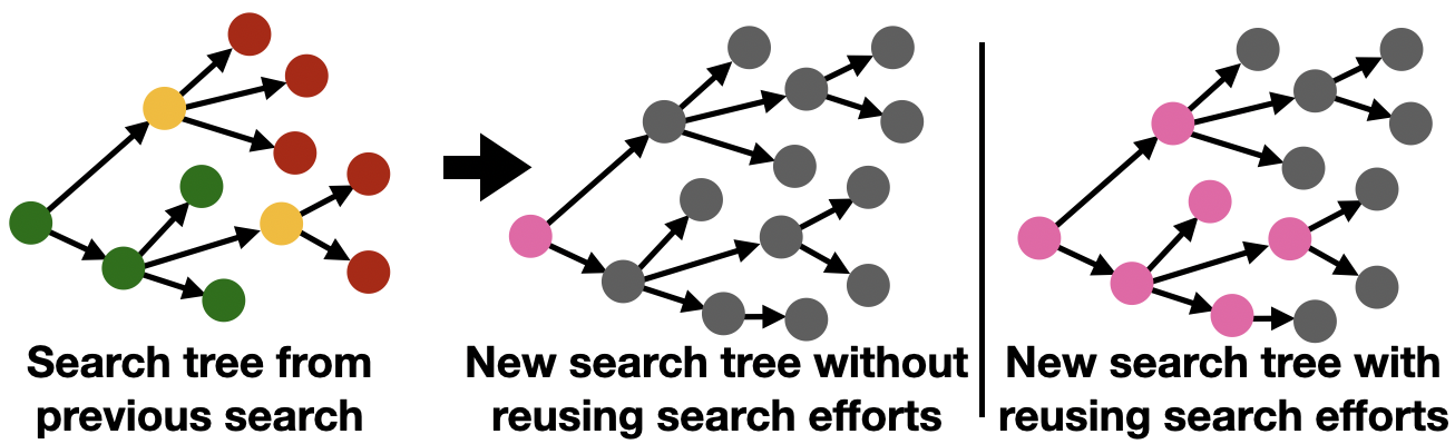
Figure 3: Visualization of how we reuse search efforts. Reusable nodes are in green, boundary nodes are in yellow and non-reusable nodes are in red. Pink nodes are obtained directly from previous search while gray nodes are newly constructed in the current search.

VI Results

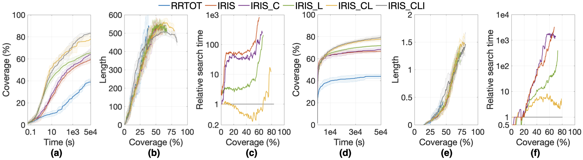
Figure 4: Result comparison of different methods. (a)–(c): Bridge inspection scenario. All variants used hyperparameters $p_{\rm accept}=0.05,p_{0}=0.85,\varepsilon_{0}=10.0$. (d)–(f): Pleural cavity inspection scenario. All variants used hyperparameters $p_{\rm accept}=0.1,p_{0}=0.9,\varepsilon_{0}=15.0$.

We evaluated our algorithmic enhancements on two simulated scenarios, a bridge-inspection task and a medical-inspection task. In each scenario, we compared the original IRIS with four variants, namely IRIS_C, IRIS_L, IRIS_CL, and IRIS_CLI, where C, L, and I stand for Coverage-informed sampling, refined Lazy edge validation, and Incremental search by reusing search efforts, respectively. For reference, we also run RRTOT [28]. Our evaluation metrics include path coverage and path length as a function of the running time, and for IRIS and its variants, we also look at the relative search efficiency compared to IRIS_CLI. We define search efficiency as, for a given inspection coverage $s$, the relative time each algorithm spends on search (and not on roadmap construction or edge evaluation) to return a path $\pi$ that satisfies $|\mathcal{S}(\pi)|\geq s$ for the first time. Search efficiency is compared only in Fig. 4 (c) and (f), while Fig. 4 (a) and (d) use the total running time.

Our implementation is based on the publicly-available C++ implementation of IRIS [52] (new code corresponding to the improvements suggested in this work are also incorporated to this repository). All experiments were run on a dual 2.1GHz 16-core Intel Xeon Silver 4216 CPU and 100GB of RAM. All experiments were run for $50,000$ seconds. The initial values of $\varepsilon,p$ are denoted as $\varepsilon_{0},p_{0}$ and we updated them with $p_{i}=p_{i-1}+f\cdot(1-p_{i-1}),\varepsilon_{i}=\varepsilon_{i-1}+f\cdot(0-\varepsilon_{i-1})$, where $f$ is a parameter controlling the tightening of the approximation factors. We used $f=10^{-4}$. Finally, additional results can be found in Appendix B.

VI-A Bridge inspection scenario

Almost $40\%$ of the bridges in the US exceed their 50-year design life [53], and regular inspections are critical to ensure bridge safety. Existing inspection methods are typically expensive, and using UAVs to autonomously inspect bridges could potentially reduce inspection time and costs. In this scenario, a UAV with a camera is tasked with inspecting a bridge (Fig. 1 top left), which includes 3,346 POIs extracted from a 3D mesh model.

The UAV’s C-space is $\mathbb{R}^{3}\times\mathcal{SO}(2)$: it may translate in 3D and rotate around its vertical axis, and the camera can further rotate around the pitch axis. The camera is modeled as having a field of view of $94$ degrees and an effective inspecting range of $10$ meters.

Fig. 4 (a), (b) show that all IRIS variants have better performance than the original IRIS since they achieve better inspection coverage faster while keeping similar plan lengths. Specifically, IRIS_CLI achieves the best performance, reaching $23\%$ more inspection coverage than the original IRIS and is $570\times$ faster in reaching a coverage of $60\%$. IRIS_CLI also achieves $44\%$ more inspection coverage than RRTOT. Fig. 4 (c) compares the speedup in graph search time of IRIS_CLI to reach a given inspection coverage comparing to other variants. As we can see, for search efficiency, IRIS_CLI is $830\times$ faster than the original IRIS for a coverage of $60\%$, and it is roughly $12\times$ faster than the second-best method, IRIS_CL, for a coverage of $78\%$.

VI-B Pleural cavity inspection scenario

A pleural effusion is a serious medical condition in which excess fluid builds up between the lungs and chest wall and can cause lung collapse. Pleural effusions may result from many different diseases, including cancer. To effectively diagnose the cause of pleural effusion, doctors need to visually inspect the inner surface of the pleural cavity, the fluid-filled space between the lungs and the chest wall. In this scenario, a CRISP robot [18, 17] with a chip-tip camera performs the endoscopic diagnosis (Fig. 1 top right). The pleural cavity is segmented from a patient Computerized Tomography (CT) scan, and we densely sample 4,203 POIs on the surface of the pleural cavity.

Composed of flexible needle-diameter tubes, the CRISP robot requires smaller incisions compared to traditional endoscopic instruments, thus reducing patient pain and shortening the recovery time. The tubes are inserted into the patient body separately and assembled into a parallel structure with snares. When manipulating the tubes outside the body, the shape of the robot inside the body changes accordingly, changing the pose of the chip-tip camera to inspect surrounding anatomy. In our scenario, we use a two-tube CRISP robot. At the entry point, each tube can rotate in three dimensions (yaw, pitch, and roll) and translate in one dimension (insert or retract). So the system has a C-space $\mathcal{C}\subseteq\mathcal{SO}(3)^{2}\times\mathbb{R}^{2}$.

The robot’s forward kinematics (FK) is computationally expensive: computing the shape of the robot requires numerical methods to model the torsional and elastic interactions between all the flexible tubes of the parallel structure [18]. Thus FK-involved procedures, including roadmap construction and edge validation during graph search, are time-consuming. In this scenario, for the initial $50\%$ coverage, the original IRIS shows better efficiency since fewer edges are validated. However, Fig. 4 (d), (e) show that as $\mathcal{G}$ grows, the performance of the original IRIS plateaus as the time spent on search begins to dominate, while other variants keep making progress. IRIS_CLI reaches $12\%$ more inspection coverage than the original IRIS and is $6\times$ faster in reaching a coverage of $67\%$. IRIS_CLI also achieves $35\%$ more inspection coverage than RRTOT. When it comes to search efficiency, Fig. 4 (f) shows IRIS_CLI is over $3,200\times$ faster than the original IRIS for a coverage of $67\%$ and $5\times$ faster than IRIS_CL for a coverage of $79\%$.

VII Conclusion & future work

In this paper, we introduced a faster inspection planning algorithm based on enhancements to IRIS. The new algorithm uses coverage-informed sampling to construct more effective roadmaps and uses two enhanced search techniques to improve the computational efficiency of the near-optimal search algorithm employed by the original IRIS. More specifically, one is refined lazy edge validation that saves computation time for search when the roadmap is densified, and the other is reusing search efforts when a roadmap undergoes local changes. Simulation experiments in two scenarios show the improved search algorithm is dramatically faster than the original one. With better computational efficiency, we can achieve similar-quality plans with significantly shorter computation time while retaining IRIS’s asymptotic optimality.

The IRIS framework can be further improved. In this work, the coverage-informed sampling method simply rejects samples to control the size of the roadmap. This yields good performance, but a more effective way of determining good viewpoints would potentially be more beneficial. A different possible approach to build a compact and informative roadmap is sparsifying the roadmap. Here we draw inspiration from roadmap sparsification techniques for motion planning (see, e.g., [54, 55]) that demonstrated how to reduce a given roadmap’s size with very little compromise on the quality of resulting plan.

Appendix A Pseudo-code

In this section we provide pseudo-code for the new improvements. To make this section self-contained, there is some text that repeats descriptions provided in the main body of this work.

A Original IRIS

Before introducing IRIS_CLI, we first briefly review the original IRIS algorithm [16]. Please note for Alg. 1 and Alg. 2, IRIS is in black and blue text, while for IRIS_CLI, green lines are added and blue lines are modified.

Let $\mathcal{C}$ be the configuration space, $\mathbf{q}_{s}$ a start configuration, $\mathcal{S}$ a sensor model, $\mathcal{I}$ a set of POIs, and $ell$ a distance metric, all as defined in Sec. III. In the original IRIS algorithm, configuration sampling and near-optimal graph search are performed in an interleaved manner (see Alg. 1).

In the sampling phase, a roadmap $\mathcal{G}$ is constructed as a Rapidly-exploring Random Graph (RRG), which is implicitly defined by a Raplidly-exploring Random Tree (RRT). Denote $\mathcal{G}=(\mathcal{V},\mathcal{E})$, where $\mathcal{V}$ is the set of all vertices and $\mathcal{E}$ is the set of all edges. Each vertex $v\in\mathcal{V}$ is a collision-free configuration $\mathbf{q}\in\mathcal{C}_{\rm free}$, whose inspection coverage is $\mathcal{S}(\mathbf{q})$, and each edge $e\in\mathcal{E}$ is the motion connecting two configurations, whose length is defined by $\ell(e)$. Since the roadmap is implicitly defined, only edges in the RRT is validated during construction. Then in the search phase, a near-optimal plan is found. A plan $\pi$ is near-optimal for some approximation parameters $p\in[0,1]$ and $\varepsilon\geq 0$ if $|\mathcal{S}(\pi)|\geq p\cdot|\mathcal{S}(\pi^{*})|$ and $\ell(\pi)\leq(1+\varepsilon)\cdot\ell(\pi^{*})$, where $\pi^{*}$ is the optimal plan on $\mathcal{G}$ that has the shortest length among all feasible trajectories that covers the maximum number of POIs.

The near-optimal graph search (Alg. 1, line 9) is a core component in IRIS’s framework. The details are shown in Alg. 2. Each node in the search is a path pair (PP) composed of an achievable path (AP) and a potentially achievable path (PAP). We denote $\textsf{PP}_{v}=(P_{v},\tilde{P_{v}})$, where $\textsf{PP}_{v}$ denotes a path pair that starts from $\mathbf{q}_{s}$ and ends at vertex $v\in\mathcal{C}$, here $P_{v}$ is an AP and $\tilde{P_{v}}$ is a PAP. For formal definitions of a PP, an AP, and a PAP, please refer to [16]. Roughly speaking, an AP is an achievable sequence of vertices, by tracing back the predecessors of the PP, such a sequence can be reconstructed; while for a PAP, there’s no way to reconstruct the sequence of vertices and we don’t even require that such a path exists. A PAP is defined by the pair $\mathcal{S}(\tilde{P_{v}})$ and $\ell(\tilde{P_{v}})$ bounding the potentially-best inspection coverage and plan length can be achieved via all paths encoded in the path pair. Note that by definition, $\ell(\tilde{P_{v}})\leq\ell(P_{v})$ and $\mathcal{S}(\tilde{P_{v}})\supseteq\mathcal{S}(P_{v})$.

Algorithm 1 Incremental Random Inspection-roadmap Search(IRIS)
Input: $\mathcal{C}$, $\mathbf{q}_{s}$, $\mathcal{S}$, $\mathcal{I}$, $p_{0}$, $\varepsilon_{0}$
Colors: modified

1:$\mathcal{V}\leftarrow\{\mathbf{q}_{s}\}$, $\mathcal{E}\leftarrow\emptyset$, $\mathcal{G}\leftarrow\left(\mathcal{V},\mathcal{E}\right)$

2:$\pi\leftarrow$ {$\mathbf{q}_{s}$}

3:$p\leftarrow p_{0}$, $\varepsilon\leftarrow\varepsilon_{0}$

4:while not TIMED_OUT do

5:   $\mathcal{G}\leftarrow$ ExpandRoadmap($\mathcal{C}$, $\mathcal{G}$, $\mathcal{I}$) $\triangleright$ Sampling

6:   $p,\varepsilon\leftarrow$ UpdateApproximation()

7:   if not NeedNewSearch($\mathcal{G}$, $\pi$, $p$) then

8:     continue    

9:   $\pi\leftarrow$ NearOptimalGraphSearch($\mathcal{G}$, $\mathbf{q}_{s}$, $p$, $\varepsilon$) $\triangleright$ Search

10:return $\pi$

We define two operations defined on PPs:

1. Extending operation: extending $\textsf{PP}_{u}$ by edge $e=(u,v)\in\mathcal{E}$ will extend both $P_{u}$ and $\tilde{P_{u}}$ by edge $e$. The result path pair is $\textsf{PP}_{v}=(P_{v},\tilde{P_{v}})$, where AP satisfies $\mathcal{S}(P_{v})=\mathcal{S}(P_{u})\cup\mathcal{S}(v),\ell(P_{v})=\ell(P_{u})+\ell(e)$, and PAP satisfies $\mathcal{S}(\tilde{P_{v}})=\mathcal{S}(\tilde{P_{u}})\cup\mathcal{S}(v),\ell(\tilde{P_{v}})=\ell(\tilde{P_{u}})+\ell(e)$. We denote the extending operation as $\textsf{PP}_{v}=\textsf{PP}_{u}+e$.

2. Subsuming operation: Subsuming between two PPs can only happen when both PPs start from the same vertex (this is non-trivial since all PPs starts from $\mathbf{q}_{s}$) and ends at the same vertex. Assume we have ${\rm PP_{1}}=(P_{1},\tilde{P_{1}})$ and ${\rm PP_{2}}=(P_{2},\tilde{P_{2}})$ both ends at vertex $v$, the result path pair of ${\rm PP_{1}}$ subsuming ${\rm PP_{2}}$ is defined as $\textsf{PP}_{1}\oplus\textsf{PP}_{2}:=\left(P_{1},\left(\mathcal{S}(\tilde{P_{1}})\cup\mathcal{S}(\tilde{P_{2}}),\min(\ell(\tilde{P_{1}}),\ell(\tilde{P_{2}}))\right)\right)$.

Subsuming is a core operation to achieve near-optimal search. The search starts with the root node $\textsf{PP}_{\mathbf{q}_{s}}=\left(\{\mathbf{q}_{s}\},(\mathcal{S}(\mathbf{q}_{s}),0)\right)$ where the PAP and AP have exactly the same inspection coverage and path length. When subsuming happens during the search, the PAP gradually increases its inspection coverage and/or decreases path length when compared to the AP. To guarantee near-optimality of the result, we ensure that all path pairs are $\varepsilon,p$-bounded. Here, a PP is said to be $\varepsilon,p$-bounded if its AP $P$ and PAP $\tilde{P}$ satisfy both $|\mathcal{S}(P)|\geq p\cdot|\mathcal{S}(\tilde{P})|$ and $\ell(P)\leq(1+\varepsilon)\cdot\ell(\tilde{P})$. By guaranteeing that all PPs in the closed set and open list are $\varepsilon,p$-bounded for the given $p$ and $\varepsilon$, Alg. 2 finds near-optimal inspection plans (see [16] for a proof sketch).

Algorithm 2 NearOptimalGraphSearch
Input: $\mathcal{G},\mathbf{q}_{s},p,\varepsilon$
Colors: modified, added

1:${\rm CLOSED},{\rm OPEN}\leftarrow$ InitializeLists($\mathbf{q}_{s},p,\varepsilon$)

2:while ${\rm{OPEN}}\neq\emptyset$ do

3:   $\textsf{PP}_{u}\leftarrow$ OPEN.extract_min()

4:   if not Valid($\textsf{PP}_{u})$ then

5:      continue $\triangleright$ Edge validation

6:   if $\mathcal{S}(\tilde{P_{u}})==\mathcal{S}(\mathcal{G}.\mathcal{V})$ then $\triangleright$ $\tilde{P_{u}}$ is the PAP of $\textsf{PP}_{v}$

7:     OPEN.insert($\textsf{PP}_{u}$) $\triangleright$ For search efforts reuse

8:     return $P_{u}$ $\triangleright$ ${P_{u}}$ is the AP of $\textsf{PP}_{u}$    

9:   for $e=(u,v)\in$ Neighbors($u,\mathcal{G}$) do

10:     $\textsf{PP}_{v}\leftarrow\textsf{PP}_{u}+e$ $\triangleright$ Extending operation

11:     AddNewNode($\textsf{PP}_{v},{\rm CLOSED},{\rm OPEN},p,\varepsilon$)    

12:   CLOSED.insert($\textsf{PP}_{u}$)

13:return NULL

When a new node $\textsf{PP}_{v}$ is generated after some other node was extended (Alg. 2, line 10), we perform the following operations to add the node while ensuring that all PPs are $\varepsilon,p$-bounded:

1. For any node $\textsf{PP}_{v}^{\prime}\in{\rm CLOSED}$ in the closed set, if $\mathcal{S}(\tilde{P_{v}^{\prime}})\supseteq\mathcal{S}(\tilde{P_{v}})$ and $\ell(\tilde{P_{v}^{\prime}})\leq\ell(\tilde{P_{v}})$, then the new node is dominated. In such cases we update the node in the closed set with $\textsf{PP}_{v}^{\prime}\leftarrow\textsf{PP}_{v}^{\prime}\oplus\textsf{PP}_{v}$.

2. If a node cannot be dominated by a node in the closed set, we check if for any node in the open list $\textsf{PP}_{u}^{\prime}\in{\rm OPEN}$, if $\textsf{PP}_{v}^{\prime}\oplus\textsf{PP}_{v}$ is $\varepsilon,p$-bounded, then the new node is dominated, we update the node in the open list with $\textsf{PP}_{v}^{\prime}\leftarrow\textsf{PP}_{v}^{\prime}\oplus\textsf{PP}_{v}$.

3. Finally if a new node cannot be dominated by any node in either the closed set or the open list, it may still subsume nodes in the open list . For any node in the open list $\textsf{PP}_{u}^{\prime}\in{\rm OPEN}$, if $\textsf{PP}_{u}\oplus\textsf{PP}_{u}^{\prime}$ is $\varepsilon,p$-bounded, $\textsf{PP}_{u}^{\prime}$ is dominated, we remove it from the open list and update $\textsf{PP}_{u}$ with $\textsf{PP}_{u}\leftarrow\textsf{PP}_{u}\oplus\textsf{PP}_{u}^{\prime}$, and have ${\rm OPEN}.{\rm insert}(\textsf{PP}_{u})$.

B Refined lazy edge evaluation

Recall that trivial (T) and non-trivial (NT) nodes are referring to PPs that did not and did subsume other PPs, respectively. Further recall that we perform edge evaluation when a T-node subsumes another node. Thus, any node popped from the OPEN list is either a (i) T-node; or an (ii) NT-node that is already checked to be valid. Thus, we add line 4-5 in Alg. 2 to reject invalid T-nodes. Moreover, Alg. 2 line 11 is also modified, checking the leading edge of a T-node when it is subsuming another node.

C Incremental search by reusing efforts across iterations

Since this part of the algorithm is already described in details in Sec. V-C, here we directly provide the pseudo-code (Alg. 3, 4) as a complement.

Algorithm 3 InitializeLists
Input: $\mathbf{q}_{s},{\varepsilon,p}$

1:if  initial search then

2:   ${\rm CLOSED}\leftarrow\emptyset$, ${\rm OPEN}\leftarrow\{\textsf{PP}_{\mathbf{q}_{s}}\}$

3:else

4:   ${\rm CLOSED},{\rm OPEN}\leftarrow$ RetrieveLatestLists()

5:for $\textsf{PP}_{v}\in{\rm CLOSED}\cup{\rm OPEN}$ do

6:   MarkNodeType($\textsf{PP}_{v}$)

7:RELEASE $\leftarrow\emptyset$

8:for $\textsf{PP}_{v}\in{\rm CLOSED}\cup{\rm OPEN}$ do

9:   if $\textsf{PP}_{v}$ is reusable then

10:     continue    

11:   ${\rm RELEASE}.{\rm insert}(\textsf{PP}_{v})$

12:   if $\textsf{PP}_{v}\in{\rm CLOSED}$ then

13:     ${\rm CLOSED}.{\rm erase}(\textsf{PP}_{v})$    

14:   if $\textsf{PP}_{v}\in{\rm OPEN}$ then

15:     ${\rm OPEN}.{\rm erase}(\textsf{PP}_{v})$    

16:for $\textsf{PP}_{v}\in{\rm RELEASED}$ do

17:   RecursivelyRelease($\textsf{PP}_{v},{\rm CLOSED},{\rm OPEN},{\varepsilon,p}$)

18:for $\textsf{PP}_{u}\in{\rm CLOSED}$ do

19:   for $e=(u,v)\in\text{Neighbors}(u,\mathcal{G})$ do

20:     if $v$ is new vertex then

21:       $\textsf{PP}_{v}\leftarrow\textsf{PP}_{u}+e$

22:       AddNewNode($\textsf{PP}_{v},{\rm CLOSED},{\rm OPEN},{\varepsilon,p}$)         

23:return ${\rm CLOSED},{\rm OPEN}$

Algorithm 4 RecursivelyRelease
Input: $\textsf{PP}_{v},{\rm CLOSED},{\rm OPEN},{\varepsilon,p}$

1:if $\textsf{PP}_{v}$ is reusable then

2:   AddNewNode($\textsf{PP}_{v},{\rm CLOSED},{\rm OPEN},{\varepsilon,p}$)

3:   return

4:else if $\textsf{PP}_{v}$ is boundary then

5:   $\textsf{PP}_{v}\leftarrow\textsf{PP}_{v}.{\rm predecessor()}+e$

6:   AddNewNode($\textsf{PP}_{v},{\rm CLOSED},{\rm OPEN},{\varepsilon,p}$)

7:for $\textsf{PP}_{v}^{\prime}\in\textsf{PP}_{v}$.subsumed_list() do

8:   RecursivelyRelease($\textsf{PP}_{v}^{\prime},{\rm CLOSED},{\rm OPEN},{\varepsilon,p}$)

Appendix B Additional Results

Here we provide a decomposition of running time of IRIS and IRIS_CLI.

A Bridge inspection scenario

The decomposition of the running time of IRIS and IRIS_CLI are shown in Fig. 5(a) and Fig. 5(b), respectively.

For the bridge-inspection scenario, edge validation is computationally cheap since the we do interpolation between configurations without considering the dynamics of the robot. From the charts, the time spent on edge validation is almost negligible compared to the time spent on roadmap construction and search. Additionally, note that with coverage-informed sampling and using the relaxation parameter $\omega$ (introduced in Sec. V-A), we need to run significantly fewer iterations to reach the same inspection coverage.

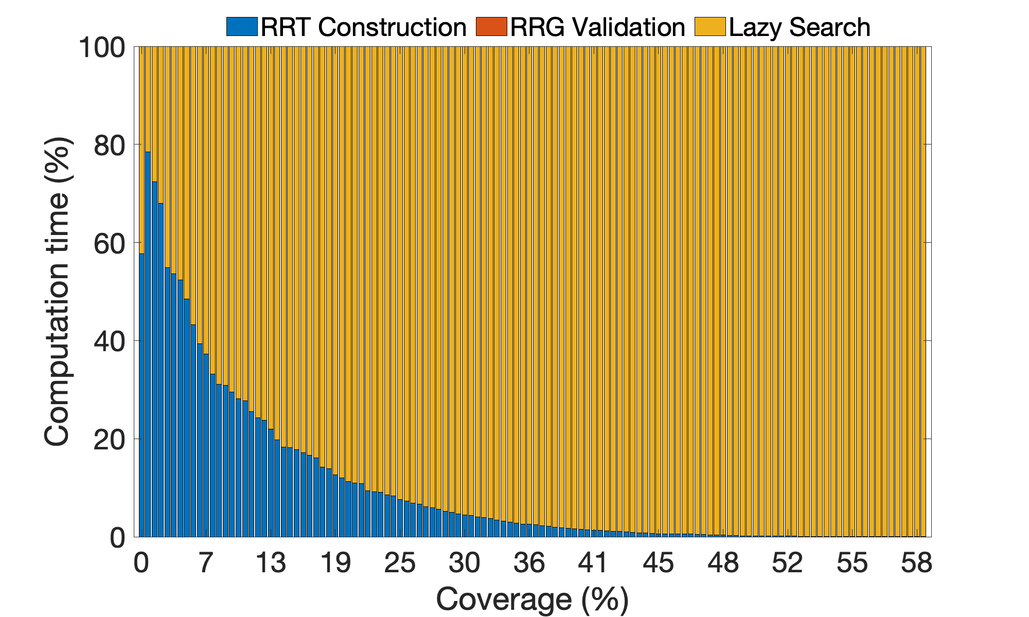
(a)

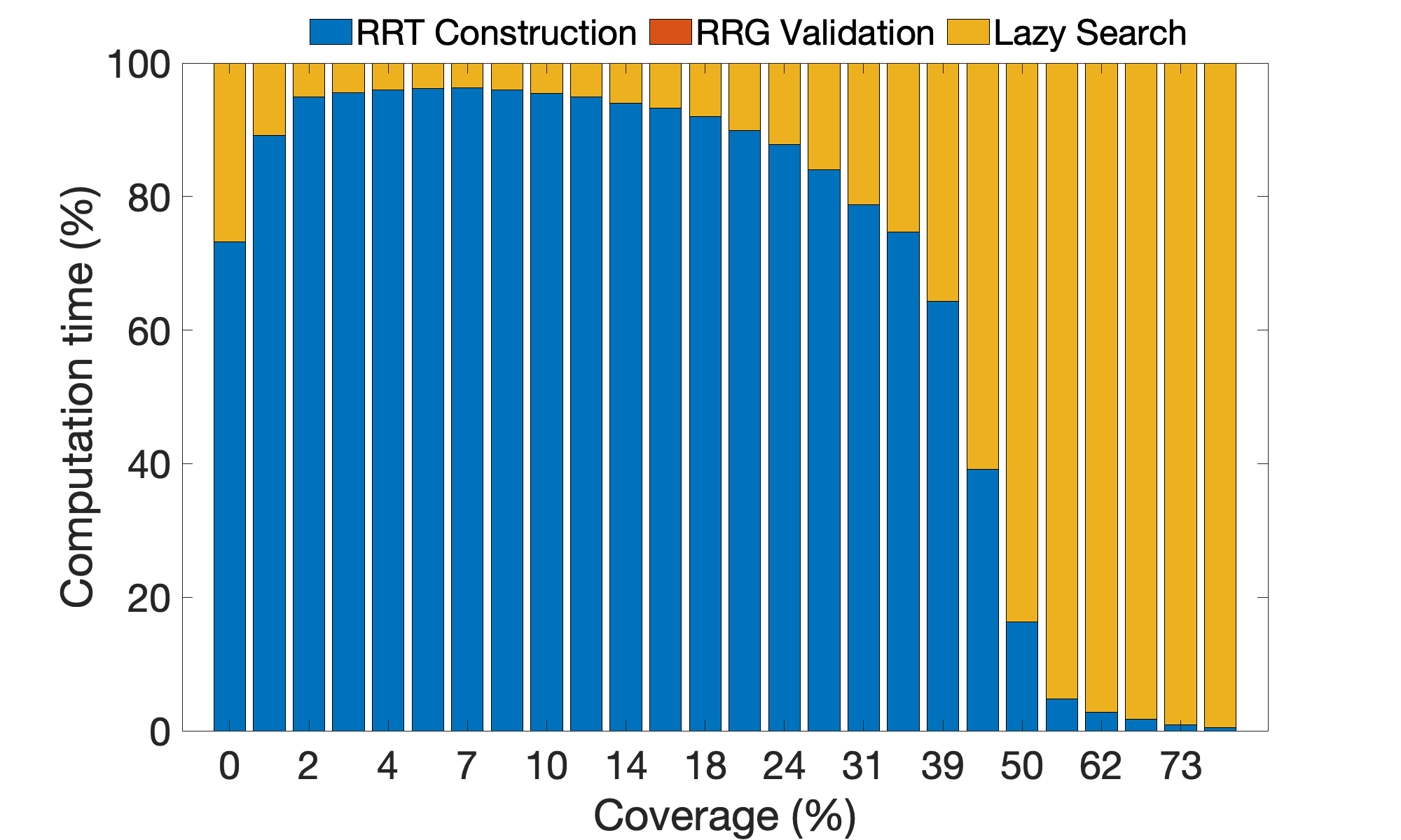
(b)

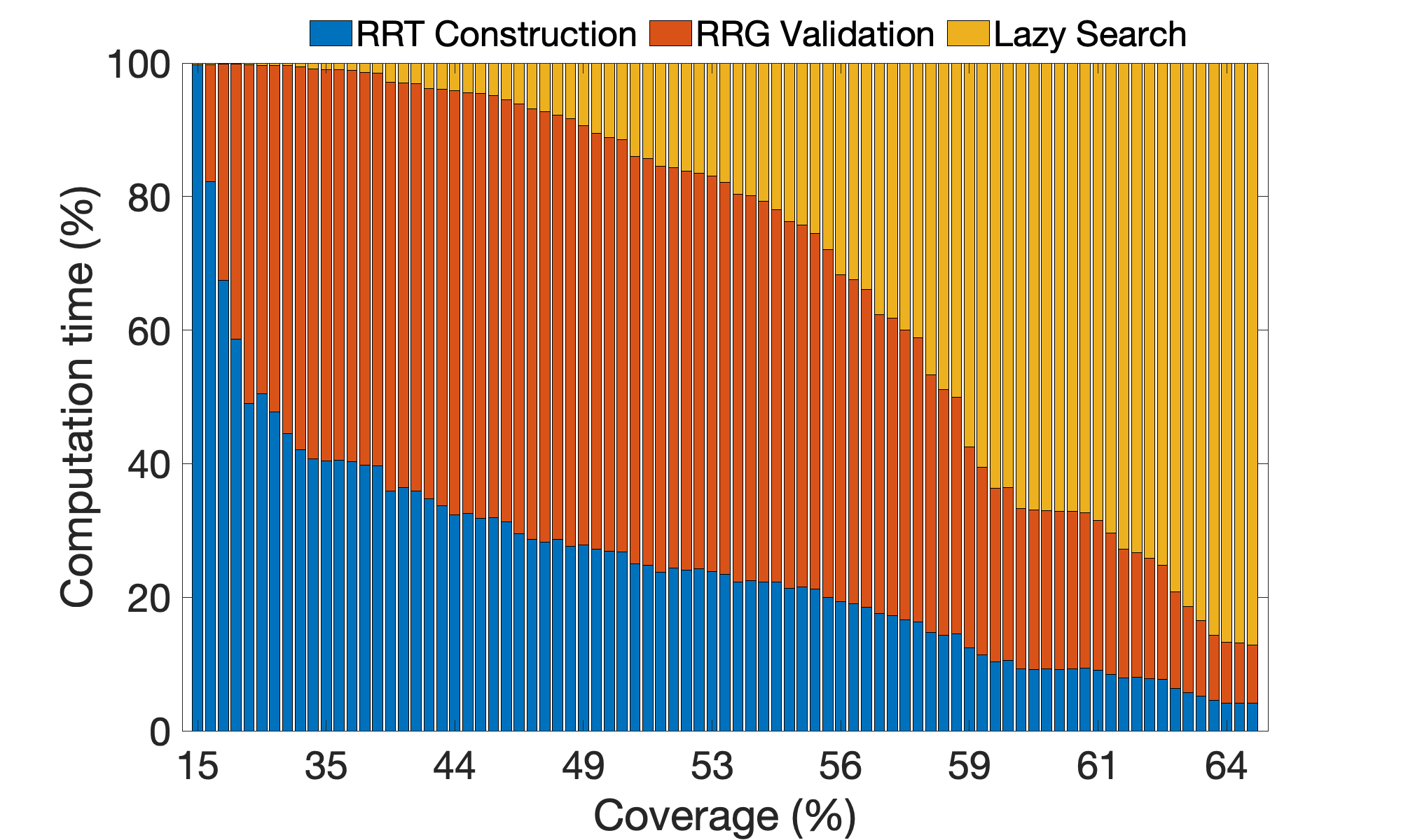
(c)

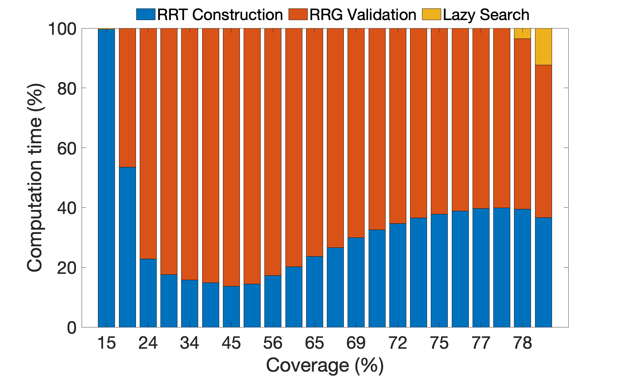
(d)

Figure 5: Running time decomposition. (5(a)) IRIS for bridge inspection scenario. (5(b)) IRIS_CLI for bridge inspection scenario. (5(c)) IRIS for pleural cavity inspection scenario. (5(d)) IRIS_CLI for pleural cavity inspection scenario.

B Pleural cavity inspection scenario

The decomposition of the running time of IRIS and IRIS_CLI are shown in Fig. 5(c) and Fig. 5(d), respectively.

For the pleural-cavity inspection scenario, edge validation is computationally expensive since the FK of the crisp robot is hard to compute. We can see from the charts that lazy search started to dominate the computation time in the original IRIS while in IRIS_CLI, the time spent on search is relatively low compared to roadmap construction and edge validation. Similar to the bridge-inspection scenario, with coverage-informed sampling and the relaxation parameter $\omega$ (introduced in Sec. V-A), we need to run significantly fewer iterations to reach the same inspection coverage.

References

- [1] R. Raffaeli, M. Mengoni, M. Germani, and F. Mandorli, “Off-line view planning for the inspection of mechanical parts,” International Journal on Interactive Design and Manufacturing (IJIDeM), vol. 7, no. 1, pp. 1–12, 2013.
- [2] P. Cheng, J. Keller, and V. Kumar, “Time-optimal UAV trajectory planning for 3d urban structure coverage,” in IEEE/RSJ Int. Conf. Intelligent Robots and Systems (IROS). IEEE, 2008, pp. 2750–2757.
- [3] A. Bircher, K. Alexis, M. Burri, P. Oettershagen, S. Omari, T. Mantel, and R. Siegwart, “Structural inspection path planning via iterative viewpoint resampling with application to aerial robotics,” in IEEE Int. Conf. Robotics and Automation (ICRA). IEEE, 2015, pp. 6423–6430.
- [4] A. Bircher, M. Kamel, K. Alexis, M. Burri, P. Oettershagen, S. Omari, T. Mantel, and R. Siegwart, “Three-dimensional coverage path planning via viewpoint resampling and tour optimization for aerial robots,” Autonomous Robots, vol. 40, no. 6, pp. 1059–1078, 2016.
- [5] R. Almadhoun, T. Taha, L. Seneviratne, J. Dias, and G. Cai, “GPU accelerated coverage path planning optimized for accuracy in robotic inspection applications,” in 2016 IEEE 59th International Midwest Symposium on Circuits and Systems (MWSCAS). IEEE, 2016, pp. 1–4.
- [6] R. Almadhoun, T. Taha, D. Gan, J. Dias, Y. Zweiri, and L. Seneviratne, “Coverage path planning with adaptive viewpoint sampling to construct 3d models of complex structures for the purpose of inspection,” in IEEE/RSJ Int. Conf. Intelligent Robots and Systems (IROS). IEEE, 2018, pp. 7047–7054.
- [7] G. A. Hollinger, B. Englot, F. Hover, U. Mitra, and G. S. Sukhatme, “Uncertainty-driven view planning for underwater inspection,” in IEEE Int. Conf. Robotics and Automation (ICRA). IEEE, 2012, pp. 4884–4891.
- [8] G. A. Hollinger, B. Englot, F. S. Hover, U. Mitra, and G. S. Sukhatme, “Active planning for underwater inspection and the benefit of adaptivity,” Int. J. Robotics Research (IJRR), vol. 32, no. 1, pp. 3–18, 2013.
- [9] B. Englot and F. S. Hover, “Three-dimensional coverage planning for an underwater inspection robot,” Int. J. Robotics Research (IJRR), vol. 32, no. 9-10, pp. 1048–1073, 2013.
- [10] B. Bingham, B. Foley, H. Singh, R. Camilli, K. Delaporta, R. Eustice, A. Mallios, D. Mindell, C. Roman, and D. Sakellariou, “Robotic tools for deep water archaeology: Surveying an ancient shipwreck with an autonomous underwater vehicle,” J. of Field Robotics, vol. 27, no. 6, pp. 702–717, 2010.
- [11] M. Johnson-Roberson, O. Pizarro, S. B. Williams, and I. Mahon, “Generation and visualization of large-scale three-dimensional reconstructions from underwater robotic surveys,” J. of Field Robotics, vol. 27, no. 1, pp. 21–51, 2010.
- [12] N. Gracias, P. Ridao, R. Garcia, J. Escartín, M. L’Hour, F. Cibecchini, R. Campos, M. Carreras, D. Ribas, N. Palomeras, et al., “Mapping the moon: Using a lightweight AUV to survey the site of the 17th century ship ‘la lune’,” in OCEANS-Bergen, 2013 MTS/IEEE. IEEE, 2013, pp. 1–8.
- [13] M. A. Tivey, A. Bradley, D. Yoerger, R. Catanach, A. Duester, S. Liberatore, and H. Singh, “Autonomous underwater vehicle maps seafloor,” Eos, Transactions American Geophysical Union, vol. 78, no. 22, pp. 229–230, 1997.
- [14] A. Kuntz, C. Bowen, C. Baykal, A. W. Mahoney, P. L. Anderson, F. Maldonado, R. J. Webster III, and R. Alterovitz, “Kinematic design optimization of a parallel surgical robot to maximize anatomical visibility via motion planning,” in IEEE Int. Conf. Robotics and Automation (ICRA), 2018, pp. 926–933.
- [15] D. Halperin, O. Salzman, and M. Sharir, “Algorithmic motion planning,” in Handbook of Discrete and Computational Geometry, Third Edition. CRC Press LLC, 2018, pp. 1311–1342.
- [16] M. Fu, A. Kuntz, O. Salzman, and R. Alterovitz, “Toward asymptotically-optimal inspection planning via efficient near-optimal graph search,” in Proceedings of Robotics: Science and Systems, FreiburgimBreisgau, Germany, June 2019.
- [17] P. L. Anderson, A. W. Mahoney, and R. J. Webster, “Continuum reconfigurable parallel robots for surgery: Shape sensing and state estimation with uncertainty,” IEEE Robotics and Automation Letters, vol. 2, no. 3, pp. 1617–1624, July 2017.
- [18] A. W. Mahoney, P. L. Anderson, P. J. Swaney, F. Maldonaldo, and R. J. Webster III, “Reconfigurable parallel continuum robots for incisionless surgery,” in Proc. IEEE/RSJ Int. Conf. Intelligent Robots and Systems (IROS), 2016, pp. 4330–4336.
- [19] B. J. Cohen, M. Phillips, and M. Likhachev, “Planning single-arm manipulations with n-arm robots,” in Robotics: Science and Systems (RSS), 2014.
- [20] T. Danner and L. E. Kavraki, “Randomized planning for short inspection paths,” in Proc. IEEE Int. Conf. Robotics and Automation (ICRA), 2000, pp. 971–976.
- [21] G. Papadopoulos, H. Kurniawati, and N. M. Patrikalakis, “Asymptotically optimal inspection planning using systems with differential constraints,” in IEEE Int. Conf. Robotics and Automation (ICRA). IEEE, 2013, pp. 4126–4133.
- [22] S. Edelkamp, M. Pomarlan, and E. Plaku, “Multiregion inspection by combining clustered traveling salesman tours with sampling-based motion planning,” IEEE Robotics and Automation Letters, vol. 2, no. 2, pp. 428–435, 2016.
- [23] I. Gentilini, K. Nagamatsu, and K. Shimada, “Cycle time based multi-goal path optimization for redundant robotic systems,” in IEEE/RSJ Int. Conf. Intelligent Robots and Systems (IROS). IEEE, 2013, pp. 1786–1792.
- [24] D.-S. Jang, H.-J. Chae, and H.-L. Choi, “Optimal control-based UAV path planning with dynamically-constrained tsp with neighborhoods,” in 2017 17th International Conference on Control, Automation and Systems (ICCAS). IEEE, 2017, pp. 373–378.
- [25] W. Jing, J. Polden, C. F. Goh, M. Rajaraman, W. Lin, and K. Shimada, “Sampling-based coverage motion planning for industrial inspection application with redundant robotic system,” in IEEE/RSJ Int. Conf. Intelligent Robots and Systems (IROS). IEEE, 2017, pp. 5211–5218.
- [26] B. Englot and F. S. Hover, “Sampling-based coverage path planning for inspection of complex structures,” in Int. Conf. Automated Planning and Scheduling (ICAPS), 2012, pp. 29–37.
- [27] B. Bogaerts, S. Sels, S. Vanlanduit, and R. Penne, “A gradient-based inspection path optimization approach,” IEEE Robotics and Automation Letters, vol. 3, no. 3, pp. 2646–2653, 2018.
- [28] A. Bircher, K. Alexis, U. Schwesinger, S. Omari, M. Burri, and R. Siegwart, “An incremental sampling–based approach to inspection planning: The rapidly–exploring random tree of trees,” Robotica, vol. 35, no. 6, pp. 1327–1340, 2017.
- [29] P. Kafka, J. Faigl, and P. Váňa, “Random inspection tree algorithm in visual inspection with a realistic sensing model and differential constraints,” in IEEE Int. Conf. Robotics and Automation (ICRA), 2016, pp. 2782–2787.
- [30] S. M. LaValle, “Rapidly-exploring random trees: A new tool for path planning,” 1998.
- [31] J. Gammell and M. Strub, “A survey of asymptotically optimal sampling-based motion planning methods,” Annual Review of Control, Robotics, and Autonomous Systems, vol. 4, no. 2021, pp. 1–25.
- [32] S. Karaman and E. Frazzoli, “Sampling-based algorithms for optimal motion planning,” Int. J. Robotics Research, vol. 30, no. 7, pp. 846–894, June 2011.
- [33] H. Choset, “Coverage for robotics – A survey of recent results,” Annals of Mathematics and Artificial Intelligence, vol. 31, pp. 113–126, 2001.
- [34] R. Almadhoun, T. Taha, L. Seneviratne, J. Dias, and G. Cai, “A survey on inspecting structures using robotic systems,” International Journal of Advanced Robotic Systems, vol. 13, no. 6, p. 1729881416663664, 2016.
- [35] P. E. Hart, N. J. Nilsson, and B. Raphael, “A formal basis for the heuristic determination of minimum cost paths,” IEEE Trans. Systems Science and Cybernetics, vol. 4, no. 2, pp. 100–107, 1968.
- [36] J. D. Gammell, T. D. Barfoot, and S. S. Srinivasa, “Informed sampling for asymptotically optimal path planning,” IEEE Trans. Robotics, vol. 34, no. 4, pp. 966–984, 2018.
- [37] D. Yi, R. Thakker, C. Gulino, O. Salzman, and S. S. Srinivasa, “Generalizing informed sampling for asymptotically-optimal sampling-based kinodynamic planning via Markov chain Monte Carlo,” in IEEE Int. Conf. Robotics and Automation (ICRA), 2018, pp. 7063–7070.
- [38] S. M. LaValle, Planning Algorithms. Cambridge, U.K.: Cambridge University Press, 2006.
- [39] R. Bohlin and L. E. Kavraki, “Path planning using lazy PRM,” in IEEE Int. Conf. Robotics and Automation (ICRA), 2000, pp. 521–528.
- [40] K. Hauser, “Lazy collision checking in asymptotically-optimal motion planning,” in IEEE Int. Conf. Robotics and Automation (ICRA), 2015, pp. 2951–2957.
- [41] L. Janson, E. Schmerling, A. A. Clark, and M. Pavone, “Fast marching tree: A fast marching sampling-based method for optimal motion planning in many dimensions,” Int. J. Robotics Research (IJRR), vol. 34, no. 7, pp. 883–921, 2015.
- [42] C. M. Dellin and S. S. Srinivasa, “A Unifying Formalism for Shortest Path Problems with Expensive Edge Evaluations via Lazy Best-First Search over Paths with Edge Selectors,” in Int. Conf. Automated Planning and Scheduling (ICAPS), 2016, pp. 459–467.
- [43] O. Salzman and D. Halperin, “Asymptotically-optimal Motion Planning using lower bounds on cost,” in IEEE Int. Conf. Robotics and Automation (ICRA), 2015, pp. 4167–4172.
- [44] N. Haghtalab, S. Mackenzie, A. D. Procaccia, O. Salzman, and S. S. Srinivasa, “The provable virtue of laziness in motion planning,” in Int. Conf. Automated Planning and Scheduling (ICAPS), 2018, pp. 106–113.
- [45] A. Mandalika, O. Salzman, and S. Srinivasa, “Lazy receding horizon A* for efficient path planning in graphs with expensive-to-evaluate edges,” in Int. Conf. Automated Planning and Scheduling (ICAPS), 2018, pp. 476–484.
- [46] A. Mandalika, S. Choudhury, O. Salzman, and S. S. Srinivasa, “Generalized lazy search for robot motion planning: Interleaving search and edge evaluation via event-based toggles,” in Int. Conf. Automated Planning and Scheduling (ICAPS), 2019, pp. 745–753.
- [47] D. Frigioni, A. Marchetti-Spaccamela, and U. Nanni, “Fully Dynamic Algorithms for Maintaining Shortest Paths Trees,” J. Algorithms, vol. 34, no. 2, pp. 251–281, 2000.
- [48] G. Ramalingam and T. Reps, “On the Computational Complexity of Dynamic Graph Problems,” Theor. Comput. Sci., vol. 158, no. 1&2, pp. 233–277, 1996.
- [49] S. Koenig, M. Likhachev, and D. Furcy, “Lifelong Planning A*,” Artificial Intelligence, vol. 155, no. 1-2, pp. 93–146, 2004.
- [50] O. Salzman and D. Halperin, “Asymptotically Near-Optimal RRT for Fast, High-Quality Motion Planning,” IEEE Trans. Robotics, vol. 32, no. 3, pp. 473–483, 2016.
- [51] J. D. Gammell, S. S. Srinivasa, and T. D. Barfoot, “Batch informed trees (BIT*): Sampling-based optimal planning via the heuristically guided search of implicit random geometric graphs,” in Proc. IEEE Int. Conf. Robotics and Automation (ICRA), May 2015, pp. 3067–3074.
- [52] M. Fu, “IRIS,” https://github.com/UNC-Robotics/IRIS, 2020, accessed: 2020-8-30.
- [53] “ASCE 2017 infrastructure report card,” https://www.infrastructurereportcard.org/wp-content/uploads/2016/10/2017-Infrastructure-Report-Card.pdf.
- [54] O. Salzman, D. Shaharabani, P. K. Agarwal, and D. Halperin, “Sparsification of motion-planning roadmaps by edge contraction,” Int. J. Robotics Res., vol. 33, no. 14, pp. 1711–1725, 2014.
- [55] A. Dobson and K. E. Bekris, “Sparse roadmap spanners for asymptotically near-optimal motion planning,” Int. J. Robotics Res., vol. 33, no. 1, pp. 18–47, 2014.