CHIMERA: A Hybrid Estimation Approach to Limit the Effects of False Data Injection Attacks

Abstract

The reliable operation of power grid is supported by energy management systems (EMS) that provide monitoring and control functionalities. Contingency analysis is a critical application of EMS to evaluate the impacts of outages and prepare for system failures. However, false data injection attacks (FDIAs) have demonstrated the possibility of compromising sensor measurements and falsifying the estimated power system states. As a result, FDIAs may mislead system operations and other EMS applications including contingency analysis and optimal power flow. In this paper, we assess the effect of FDIAs and demonstrate that such attacks can affect the resulted number of contingencies. In order to mitigate the FDIA impact, we propose CHIMERA, a hybrid attack-resilient state estimation approach that integrates model-based and data-driven methods. CHIMERA combines the physical grid information with a Long Short Term Memory (LSTM)-based deep learning model by considering a static loss of weighted least square errors and a dynamic loss of the difference between the temporal variations of the actual and the estimated active power. Our simulation experiments based on the load data from New York state demonstrate that CHIMERA can effectively mitigate 91.74% of the cases in which FDIAs can maliciously modify the contingencies.

I Introduction

In electric power grids, energy management systems (EMS) provide situational awareness and assist the decision-making. EMS encompasses hardware/field components at geographically dispersed locations and telecommunications systems, as well as software applications at utility control centers, e.g., state estimation and contingency analysis. Specifically, the network topology processor within EMS utilizes breaker status and acquired data from telemetry devices to update the power system model. The collected measurements and the updated system model facilitate the state estimator to determine the current system states. The estimated results are required by other EMS applications such as contingency analysis and optimal load flow algorithms. Thus, the accuracy EMS applications depends on the results of state estimation.

As part of state estimation routines, bad data detection (BDD) units are used to identify anomalous measurements. However, it has been shown that false data injection attacks (FDIAs) can bypass BDD [1]. Undetectable FDIAs under the situation of sensor failures could even worsen the estimation performance [2]. In addition, the conditions of the 2015 attack on the Ukrainian grid, demonstrated that the threat model of FDIAs could result in massive blackouts [3].

Contingency analysis is one of the core applications in EMS which evaluates the impact of the planned or unplanned problems that occur in the electric grid such as scheduled maintenance and component failures. Components refer to generators, transmission lines, transformers, circuit breakers, etc. According to the North American Electric Reliability Corporation (NERC), the fundamental criterion of $N-1$ (where $N$ refers to the total number of components) requires that the power system is able to withstand the disruption of one component outage [4]. Contingency scenarios can be extended to $N-k$, which refers to a number of $k$ component failures. Grid operators rely on contingency analysis to recognize system overload conditions, rank the severity of the overloaded components, and isolate them if necessary to prevent cascading failures. However, the reliability of contingency algorithms cannot be guaranteed when the system is under FDIAs [5].

To detect the FDIAs, two major detection approaches are considered [6], model-based and data-driven methods. Model-based methods leverage system physics and data (e.g., the grid topology and lines admittance) to estimate states with methods such as recursive weighted least square and Kalman filters [7, 8]. In order to determine whether or not an attack occurs, different tests are applied to the estimation results such as the large normalized residual [9], and the cumulative sum test [8]. However, such methods are typically computationally expensive in terms of processing time and scalability [10]. On the other hand, despite the benefits of data-based approaches in terms of short execution times [11], such techniques require a large set of training data to achieve good performance. In addition, the rise of learning-based schemes in many applications is accompanied with important security challenges: it creates an incentive among adversaries to exploit potential vulnerabilities of the algorithms [12, 13]. Recent works illustrated that combining the physics- with data- based models provides several advantages, especially in terms of security, as they tightly confine the solution scope and limit the capability of the adversarial examples [14, 15].

In this paper, we study the impacts of FDIAs and propose a hybrid, model-based and data-driven, attack-resilient state estimator to mitigate the attack impact on the contingency analysis results. To the best of our knowledge, this paper is the first study to propose a hybrid estimation approach on how to mitigate the effect of FDIAs on contingency analysis. Our contributions are summarized as follows:

• We formulate an attack model to bypass state estimation BDD and cause, via FDIAs, non-critical transmission lines, i.e., lines not included in the contingency screening, to surpass their power flow limits. We show that the FDIAs impact can effectively distort the number of system contingencies.

• To mitigate the attack impact, we propose CHIMERA, a hybrid attack-resilient state estimator. i.e., a physics-informed estimator constructed based on Long Short Term Memory (LSTM) networks. It embeds the grid observation model of power flow equations into neural networks. We exploit the static and dynamic features of the observation model to construct spatial-temporal correlations among measurements, and limit how FDIAs against state estimation can affect subsequent EMS contingency results.

• We conduct simulation experiments based on load data from New York state. The results demonstrate that CHIMERA can effectively mitigate 91.74% of the attack cases in which FDIAs can maliciously modify the contingency results.

The rest of this paper is as follows: Section II provides background information. Section III discusses our attack model, and Section IV presents the mitigation strategy. Experiments are shown in Section V. Section VI draws concluding remarks.

II Background

II-A State estimation

In the nonlinear (AC) state estimation of power systems, state variables are determined by phase angles ($\theta$) and voltage magnitudes ($V$). For a system with $n$ buses, the states are $\mathbf{x}=\left[\theta_{2},\theta_{3},\ldots,\theta_{n},V_{1},\ldots,V_{n}\right]^{T}$, where $\theta_{1}=0$ is the reference angle. To maintain full observability of the system, $m\geq n$ measurements are required. Measurements ($\mathbf{z}$) typically include active power ($P$) and reactive power ($Q$) measurements. The relationship between states and acquired measurements, with $\mathbf{e}$ being a vector of noises, is as follows:

$$\mathbf{z}=\mathbf{{h}}(\mathbf{x})+\mathbf{e}\vspace{-1mm}$$ (1)

State estimation is widely solved via iterative techniques such as the weighted least square method [16], in which the accuracy of the estimated variables ${\mathbf{x}}$ is calculated via the Euclidean norm of the residual $\lVert\mathbf{z}-\mathbf{h}(\hat{\mathbf{x}})\rVert$. For example, the estimated states $\mathbf{\hat{x}}$ can be obtained through optimization of $J(\mathbf{\hat{x}})$ in Eq. (2), where $\mathbf{W}=\operatorname{diag}\left\{\sigma_{1}^{-2},\sigma_{2}^{-2},\cdots,\sigma_{m}^{-2}\right\}$.There are different approaches to solve Eq. (2); one such method is via iteratively solving Eq. (3). To detect whether or not the state estimation is disturbed by the random noises or attacks, BDD compares the objective function $J(\mathbf{\hat{x}})$ with a normalized threshold $\tau$. If $J(\mathbf{\hat{x}})<\tau$, no bad data is detected.

$$\min_{\hat{x}}J(\mathbf{\hat{x}})=(\mathbf{z}-\mathbf{h}(\mathbf{{\hat{x}}}))^{T}\mathbf{W}(\mathbf{z}-\mathbf{{h}({\hat{x}}))}$$ (2)

$$\mathbf{H}^{T}_{k}\mathbf{W}\mathbf{H}_{k}\Delta{\mathbf{\hat{x}_{k}}}=\mathbf{H}^{T}_{k}\mathbf{W}[\mathbf{z}-\mathbf{h}(\mathbf{\hat{x}_{k}})]\vspace{-1mm}$$ (3)

To reduce the computational overhead, linear (DC) state estimation is often adopted which assumes that transmission line resistances are negligible, voltage magnitudes are 1 per unit, and the differences in voltage angles between buses are small. Thus, the observation model can be linearized:

$$P_{i}=\sum\nolimits_{j\in N_{i}}{\mathbf{B}_{ij}}(\theta_{i}-\theta_{j}),\vspace{-1mm}$$ (4)

and in matrix form $\mathbf{P}=\mathbf{H}\bm{\theta}$, in which $\mathbf{P}$ and $\bm{\theta}$ are the vectors of the active power measurements and the voltage angles of the buses, respectively. $\mathbf{H}$ is the measurement Jacobian matrix derived from the susceptance matrix $\mathbf{B}$. With the approximations, the accuracy of the estimation is decreased while the computation overhead is reduced. The states $\bm{\theta}$ can be estimated with the following equation:

$${\tilde{\bm{\theta}}}=(\mathbf{H}^{T}\mathbf{H})^{-1}\mathbf{H}^{T}\mathbf{P}\vspace{-1mm}$$ (5)

II-B Contingency Analysis

Contingency analysis simulates the effects of contingency/outage scenarios and calculates the overload conditions. However, the computational cost of such “what-if” scenarios is unrealistic for large-scale and complex power systems. The computational overhead is proportional to $N!/[k!(N-k)!]$ for $N-k$ contingencies. Due to the low probability of $N-3$ contingencies occurring in different transmission lines in real-world [17], research works typically focus on $N-1$ and $N-2$ scenarios [18]. In order to find all power flow constraint violations under $N-1$ and $N-2$ scenarios, the linear power flow approximation is typically utilized [19]. Following such approach, in this work, the power flows are calculated by $\mathbf{f}=\mathbf{Y}\mathbf{M}^{T}\bm{\theta}$, where $\mathbf{Y}$ is the branch susceptance matrix, $\mathbf{M}$ is the connection matrix, and $\bm{\theta}$ is the vector of voltage phase angles. Additionally, $\mathbf{f}$ is used to calculate the line outage distribution factors (LODFs). LODFs determine the power flow impact on the remaining lines when one or more line outages are observed in the system. The formulation of single and double outages can be found in [20].

III Attack Model

III-A Threat Model

FDIAs have been traditionally demonstrated on how to compromise the state estimation [6]. In this paper, we assume that the attacker does not solely target to falsify the state estimation but also to manipulate the contingency analysis results [21]. We consider an attacker who can exploit the configuration of a power system to launch FDIAs by manipulating the sensor measurements while bypassing BDD. Moreover, the attacker targets those measurements which could distort the number of contingencies. The assumptions of the threat model are as follow:

• The attacker has full observation of the topology and configurations of the system, i.e., the attackers could construct the Jacobian matrix $\mathbf{H}$. Such data can be obtained through public information or signal reconstruction [22, 23].

• The attacker is aware of the specifics of the state estimation process, either model-based or data-driven, in order to carefully craft FDIAs to bypass BDD routines.

• The attacker has access to the real-time measurements of deployed grid sensors, e.g., via eavesdropping on the communication links. However, due to the limited physical access or the protection of certain meters, the attacker can compromise a limited number of measurements [16].

• The attacker could perform contingency analysis based on the estimated results and the power flow constraints of each line required to ensure an overload condition [18].

III-B Mathematical Formulation

Despite BDD mechanisms can detect measurement anomalies, carefully crafted FDIAs can bypass such algorithms. Consider the malicious vector $\mathbf{a}$ injected into measurements $\mathbf{z}$, then the compromised vector can be represented as $\mathbf{z_{a}}=\mathbf{z}+\mathbf{a}$. The attacked estimated state variables can be written as $\mathbf{\hat{x}_{a}}=\mathbf{\hat{x}}+\mathbf{c}$, where $\mathbf{c}$ is the vector of the injected and resulted error. A successful FDIA undetected by the residual-based BDD, as shown in Eq. (6), can be formed when $\mathbf{a}=\mathbf{Hc}$, i.e., if $\mathbf{a}$ is a linear combination of $\mathbf{H}$, for the arbitrary vector $\mathbf{c}$.

$$\lVert{r_{a}}\rVert =\left\|\mathbf{z_{a}}-\mathbf{H}(\mathbf{\hat{x}_{a}})\right\|$$ (6)

$$=\left\|\mathbf{z}+\mathbf{a}-\mathbf{H}(\mathbf{\hat{x}}+\mathbf{c})\right\|$$

$$=\left\|\mathbf{z}+\mathbf{H}(\mathbf{\hat{x}}+\mathbf{c})-\mathbf{H}(\mathbf{\hat{x}})-\mathbf{H}(\mathbf{\hat{x}}+\mathbf{c})\right\|$$

$$=\|\mathbf{z}-\mathbf{H}(\mathbf{\hat{x}})\|=\lVert r\rVert$$

Fig. 1 depicts the overall process of the attack model. The sensor measurements $\mathbf{z}$ are compromised by FDIAs represented by an attack vector $\mathbf{a}$. The estimated states $\mathbf{\hat{x}}$, as the output of the estimation process, will be altered under FDIAs. The BDD can detect and remove the significant errors as bad data, namely $J\mathbf{(\hat{x})}$ above the threshold $\tau$. Otherwise, if BDD is bypassed due to FDIAs, the malicious states will be processed to perform contingency analysis. Since the power flow computation, $\mathbf{f^{a}}$, is affected, the contingency results $\mathbf{f^{a}}^{\prime}$ will be inaccurate. As a result, system operators will be misled by the malicious contingency analysis output, and thus, potential threats to the power system reliability may be posed.

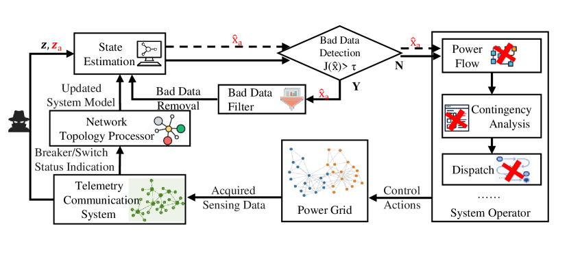
Figure 1: Illustration of the attack model (attacked variables in red color).

Based on the assumptions of the attacker’s capabilities and knowledge of the power system topology and data, the attack model is mathematically formulated as Eq. (1) - (1), where the attacker’s objective is to affect the results of contingency analysis by FDIAs. In order to achieve that, the attacker performs contingency analysis to obtain the power flows under contingency and find the most vulnerable line $i$ which has the smallest difference between its power flow under contingency ${{f_{i}^{\mathbf{a}}}^{\prime}}$, and its power flow capacity $f^{limit}_{i}$. The targeted line will overload based on the maximization function with an optimal attack vector $\mathbf{a}$ through FDIAs, as shown in Eq.(1). An absolute value of ${{f_{i}^{\mathbf{a}}}^{\prime}}$ is used here to represent the overflow observed either with ${{f_{i}^{\mathbf{a}}}^{\prime}}>f^{limit}_{i}$ or $-{{f_{i}^{\mathbf{a}}}^{\prime}}>f^{limit}_{i}$.

In order for the FDIAs to be stealthy and not being detected, several constraints represented by Eq. (1) - (1) should be satisfied. In practice, a safety margin $f_{m}$ in the line flow capacity is reserved to reduce the overload risk. Therefore, only the line with a power flow below the certain line flow capacity ${f^{limit}_{i}}-f_{m}$ will be considered, as described in (1). Eq.(1) shows that the attacker can compromise certain measurement $\mathbf{z}$ to $\mathbf{z_{a}}$ by adding an attack vector $\mathbf{a}$. Accordingly, the estimated state variables $\mathbf{\hat{x}}$ will be deviated to $\mathbf{\hat{x}_{a}}$ in (1). In order to maintain stealth and bypass the BDD, the injected error should guarantee that the residual $J(\mathbf{\hat{x}_{a}})$ is within the system threshold $\tau$, as depicted in (III-B). Once the malicious state variables are utilized to perform power flow computations, the results $\mathbf{f^{a}}$ will be affected since the voltage phase angles $\bm{{\hat{\theta}_{\mathbf{a}}}}$ in (1) are part of the deviated estimated variables $\mathbf{\hat{x}}$. The factor $\lambda^{\mathbf{a}}$ to qualify the line overload condition, LODF, will be utilized to compute the power flows. Taking the compromised power flow equation at line $i$ (${f_{i}^{\mathbf{a}}}$), line $j$ (${f_{j}^{\mathbf{a}}}$) with the LODF, the power flow of line $i$ under FDIAs with line $j$ during a outage is derived as ${{f_{i}^{\mathbf{a}}}^{\prime}}$ in (1).

—l—[2] a argmin_—f^a_i^′— f^limit_i - —f^a^′_i— —f^a^′_i—¡ f^limit_i - f_m z_a=z+a ^x_a=^x + c J(^x_a)¡τ f^a=Y M^T ^θ_a f_i^a^′=λ_i j^a f_j^a + f_i^a

IV CHIMERA: Hybrid Attack-Resilient Estimator

In order to mitigate the impacts of FDIAs on the state estimation and the consequential contingency analysis, we propose CHIMERA, a hybrid attack-resilient state estimator. CHIMERA is an AC state estimator, which takes active and reactive power measurements as well as DC-estimated voltage angles as the input, and provides estimates of voltage magnitudes and angles of the buses. Given the attack model presented in Section III and considering that a DC power flow model is typically used in grid operations [6], we build an AC hybrid estimator which is resilient to FDIAs affecting EMS routines. Despite a corrupted DC estimation output $\tilde{\bm{\theta}}_{t}$, CHIMERA provide accurate state predictions, by taking advantage of both the observation model Eq. (1) and an LSTM-based deep learning model. The LSTM network can capture the temporal correlations between data, and thus, the errors induced by the attacks can be corrected by the historical information. Moreover, since the observation model can confine the solution space with the physical constraints, we construct the loss function based on such a model.

In regards to the enhancement of the convergence speed and the estimation accuracy, we provide the DC estimation results ${\tilde{\bm{\theta}}}$ as the input of CHIMERA in addition to the power measurements ($\mathbf{P}$, $\mathbf{Q}$). Despite the limited accuracy of the DC estimation results due to the approximations, the DC estimated voltage angles can directly infer the scope of the true voltage angles. Thus, even in the presence of FDIAs, we include the DC estimated voltage angles in the input of CHIMERA because they can partially represent the states of the power grid. As a result, the input is formulated as $\mathbf{u}_{t}=[\mathbf{z}_{t};\tilde{\bm{\theta}}_{t}]$, in which $\mathbf{z}_{t}$ and $\tilde{\bm{\theta}}_{t}$ are the vectors of the sensor measurements and the DC estimated states at time $t$, respectively.

To capture the spatio-temporal correlations of the observation model in the presence of benign and malicious data, the loss function of CHIMERA is composed of two parts: the static loss and the dynamic loss. In general, to regulate the accuracy of the estimated states, a typical way is to use the difference between the observed measurements and the derived measurements from the observation model Eq. (1) [15, 12], which is defined as the static loss:

$$L_{static}=MSE({\mathbf{z}_{t}},\mathbf{h}({\hat{\mathbf{x}}_{t}})),$$ (7)

in which $\hat{\mathbf{x}}_{t}=[\hat{\bm{\theta}}_{t};\hat{\mathbf{V}}_{t}]$ is the vector of estimated states from the model. $MSE(\mathbf{x},\mathbf{y})=(1/n)\sum_{i=1}^{n}\left(x_{i}-y_{i}\right)^{2}$ is the Mean Squared Error (MSE) between $\mathbf{x}$ and $\mathbf{y}$. Nevertheless, with only $L_{static}$, the LSTM network cannot totally mitigate the impacts of FDIAs, especially on contingency analysis. Although the structure of LSTM can utilize the temporal correlations of data implicitly, adversarial perturbations including FDIAs on such recurrent neural networks have been proven effective [11]. Therefore, as also shown in Section V, depending solely on the temporal correlations from LSTM is insufficient to defend against the attack proposed in Section III. To better describe the temporal correlations between data, we further exploit the consistency of the observation model in the time domain and explicitly augment the loss function with the dynamic loss, $L_{dynamic}$. The dynamic loss measures the distance between the expected and the actual variations of the measurements. Given Eq. (4), we have:

$$\mathbf{P}_{t}-\mathbf{P}_{t-1}=\mathbf{H}(\hat{\bm{\theta}}_{t}-{\tilde{\bm{\theta}}}_{t-1}),$$ (8)

in which $\hat{\bm{\theta}}_{t}$ is the vector of the phase angles estimated by CHIMERA. Denote $\mathbf{\Delta{P}}_{t}=\mathbf{P}_{t}-\mathbf{P}_{t-1}$ and $\mathbf{\Delta\hat{{P}}}_{t}=\mathbf{H}(\hat{\bm{\theta}}_{t}-\tilde{\bm{\theta}}_{t-1})$. Thus the dynamic loss is defined as:

$$L_{dynamic}=MSE(\mathbf{\Delta{P}}_{t},\mathbf{\Delta\hat{{P}}}_{t}).$$ (9)

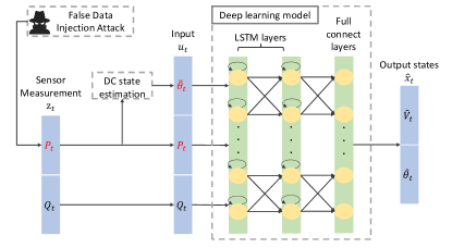
Figure 2: The architecture of CHIMERA. The variables with red color are the ones that can be affected by FDIAs.

The static loss, $L_{static}$, guarantees that the observation model is satisfied at each epoch, and the dynamic loss, $L_{dynamic}$, enforces the temporal consistency between the estimated states and the system measurements. Given $L_{dynamic}$ and $L_{static}$, the loss function of CHIMERA is defined as:

$$L=L_{static}+\gamma L_{dynamic},$$ (10)

where $\gamma\leq 1$ is the weight to balance the two terms. Compared with the loss function directly using the MSE between the estimated states and the true states, i.e., $L_{0}=MSE(\hat{\mathbf{x}},\mathbf{x})$ ($\mathbf{x}$ is the vector of the true states), the proposed loss function $L$ has several advantages. The true state $\mathbf{x}$ is not required in $L$. Note that solving $\mathbf{x}$ is non-trivial. The weighted least square method usually utilizes iterative methods to recursively minimize the residual $J(\mathbf{x})$ in Eq. (2), which is often time-consuming, especially when the grid size increases. Therefore, the utilization of $L_{static}$ and $L_{dynamic}$ can boost timing performance while estimating the true system states. Besides, as mentioned in Section II-B, the accuracy of contingency analysis heavily relies on the accuracy of the estimated variables. Since $L_{static}$ measures the difference between estimated and true power flows, $L_{static}$ can enhance the accuracy of contingency results by enforcing the consistency between the estimated and true power flows. Unlike other approaches focusing on FDIA detection, CHIMERA is ‘fertilized’ with the resilient estimation capability. This ensures that CHIMERA remains secure against other formulations of FDIAs because the attack impact will be restrained as long as the accuracy of the estimation process is guaranteed.

The architecture of CHIMERA is depicted in Fig. 2. To avoid over-fitting, validation data is utilized to select the most suitable hyper-parameters for CHIMERA. We run CHIMERA with different configurations and select the one with the most accurate estimations on the validation data. The detailed configuration is explained as follows. CHIMERA is composed of two LSTM layers and a full connection layer. For each LSTM layer, the number of the features in the hidden state is 128 and the length of the sequence is 32. For the loss function, we set $\gamma=$1\text{\times}{10}^{-3}$$. During the training phase, a batch of vectors $\mathbf{u}_{t}$ with batch size 32 are provided as input. The outputs from the output layer $\mathbf{\hat{x}}_{t}$ are then used to calculate the loss based on Eq. (10). The weights and the biases of the model are updated with the gradient of $L$ by the Adam algorithm [24], through the back-propagation process. Due to the non-linearity of the observation model in Eq. (1), there are many local minimums. To approach the global minimum of $L$, we train the model with two steps. We first train a coarse model with a large learning rate $1\text{\times}{10}^{-3}$ for 150 iterations. Then the model is fine-tuned for 500 iterations with small learning rates varying following a triangular cycle, which linearly increases from $1\text{\times}{10}^{-7}$ to $1\text{\times}{10}^{-4}$ and then decreases back to $1\text{\times}{10}^{-7}$.

V Evaluation and Simulation Results

V-A Experimental Setup

V-A1 Dataset

To examine the impacts of FDIAs on contingency analysis, we compare the number of contingencies and the overload conditions when the system is operated in normal conditions and under FDIAs. We conduct the experiment based on the IEEE 14-bus system and use synthetic data generated from the load data provided by the New York Independent System Operator (NYISO). We use NYISO load data from May 2020 containing the 5-min-interval active powers at each NY region, with 9030 epochs in total. The synthetic data is generated according to [14], and due to the unavailability of reactive power information, we generate the reactive power data by assuming a constant power factor of 0.8. White Gaussian noises with means of 0 and standard deviations of 0.01 are added to the measurements. We regard the measurements and the states generated as the ground truth when evaluating the performance of the estimation model. When executing contingency analysis, we use the flow limits listed in [25].

V-A2 Deep Learning Models for Evaluation

In addition to CHIMERA, we train two models for comparison purposes: a Multilayer Perceptron (MLP) network and the model proposed in [15]. Since MLP induces limited computational overhead, it has been widely applied to the power grid [26]. In this paper, we train a MLP network as the performance baseline. The MLP is composed of three hidden layers with 128 neurons for the first two layers and 64 neurons for the last hidden layer. We use $L_{0}=MSE(\hat{\mathbf{x}},\mathbf{x})$ as the loss function of MLP. Therefore, no additional information or system dynamics are leveraged to defend against FDIAs. We refer to this model as the baseline MLP and use it to demonstrate the impacts of FDIAs when no defense is considered. Besides the baseline MLP, we also utilize for comparison the physics-guided deep learning network proposed in [15], which encompasses an autoencoder based on LSTM and uses $\mathbf{z}_{t}$ as the input and $L_{static}$ as the loss function. We refer to this model as LSTM_ref.

The MLP and LSTM_ref are trained by following the same procedure as CHIMERA, i.e., 70% of the data is used for training, 15% for validation, and 15% for testing. The training times of the three models, deployed on a computing platform with an NVIDIA GTX 2048 and an eight-core Intel(R) Xeon(R) CPU of 2.60 GHz, are summarized in Table I. Because of the simple network architecture and loss function, the baseline MLP is trained faster than the other two models with a total time consumed for training to be 358.75s. CHIMERA makes a trade-off between training speed and security guarantees. It is trained slower than the other models, i.e., 1191.96s, because additional computations are conducted in the calculation of loss functions.

TABLE I: Training time of the baseline MLP, LSTM_ref, and CHIMERA.

Model	Coarse train (s)	Fine tune (s)	Total time (s)
MLP	101.56	257.19	358.75
LSTMref	218.48	889.9	1108.38
CHIMERA	233.09	958.87	1191.96

V-A3 Attack Setup

We select the measurements to attack based on the criticality of buses calculated according to [27]. The buses 1, 2, 3, 4, 5 have the highest criticality. Thus, the meters on those buses are selected in order for the active power measurements to be injected with errors. The optimal attack vector of Eq. (1) - (1) is solved by the Adam algorithm with a learning rate of $1\text{\times}{10}^{-2}$. The attack vector is generated for the measurement vector at each epoch. We observe that more than 99% of the estimation result residuals from the three models are smaller than $0.5$. Thus, the threshold of $J(\mathbf{\hat{x}})$ is set as $\tau=0.5$ in the attack model. We run the attacks for different values of $f_{m}$ and select $f_{m}=3$ based on the magnitudes of the injected errors. The injected errors have similar magnitudes for all three models. For each targeted measurement, the injected errors result in a Mean Absolute Error (MAE) of $0.55$ for the baseline MLP, $0.54$ for LSTM_ref, and $0.54$ for CHIMERA.

V-B Evaluation of the Estimation Results without Attacks

V-B1 Estimation Accuracy

Denote the vectors of true states and estimated states at epoch $t$ as $\mathbf{x}_{t}=[\bm{\theta}_{t};\mathbf{V}_{t}]$, and $\hat{\mathbf{x}}_{t}=[\hat{\bm{\theta}}_{t};\hat{\mathbf{V}}_{t}]$, respectively. Here $\bm{\theta}_{t}$, $\hat{\bm{\theta}}_{t}$, $\mathbf{V}_{t}$ and $\hat{\mathbf{V}}_{t}$ are the vectors of the true/estimated angles and magnitudes, respectively. We use the Mean Absolute Percentage Error (MAPE):

$$MAPE(\mathbf{x},\mathbf{y})=\frac{1}{n}\sum_{i=1}^{n}\left|\frac{y_{i}-x_{i}}{x_{i}}\right|,$$ (11)

as the accuracy evaluation metric of the estimated states, and define $MAPE\_\theta=MAPE(\bm{\theta}_{t},\hat{\bm{\theta}}_{t})$, $MAPE\_V=MAPE(\mathbf{V}_{t},\hat{\mathbf{V}}_{t})$ and $MAPE\_Total=MAPE(\mathbf{x}_{t},\hat{\mathbf{x}}_{t})$. The results are summarized in Fig. 3. Since the voltage angles fluctuate greater than the voltage magnitudes, the MSE of the angle estimations are larger than the MSE of the magnitude estimations. All three models achieve satisfiable accuracy with the average MAPEs of the states to be 1.02% for the baseline MLP, 1.70% for LSTM_ref, and 1.76% for CHIMERA.

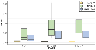
Figure 3: MAPE of the estimated states from the baseline MLP, LSTM_ref, and CHIMERA in the attack-free case.

V-B2 Contingency Analysis Results

Given the estimated states from the three models, we perform contingency analysis to reveal the variance of the numbers of $N-1$ and $N-2$ contingencies in the system. By plugging the estimated states $\hat{\mathbf{x}}_{t}$ into Eq. (1), we obtain the power flows $\hat{\mathbf{f}}_{t}$. The number of the $N-1$ and the $N-2$ contingencies at epoch $t$ given the estimated power flows $\hat{\mathbf{f}}_{t}$ are denoted as $\hat{N}_{1,t}$ and $\hat{N}_{2,t}$, respectively. Moreover, the contingency analysis based on the system measurements $\mathbf{z}_{t}$ at each epoch $t$ is executed to obtain the exact numbers of $N-1$ and $N-2$ contingencies in the system, which are denoted as ${N_{1,t}}$ and ${N_{2,t}}$, respectively. ${N_{1,t}}$ and ${N_{2,t}}$ are referred to as the ground truth.

We use the absolute errors between the aforementioned methods of acquiring the contingency data, indicated with $\epsilon_{1}=|\hat{N}_{1,t}-{N_{1,t}}|$ and $\epsilon_{2}=|\hat{N}_{2,t}-{N_{2,t}}|$, as the metric to evaluate the performance of the three models in the attack-free case. The results are shown in Fig. 4. Because of the estimation errors, errors are introduced into the contingency analysis results inevitably. The results demonstrate the benefit of $L_{static}$ over $L_{0}$. Although the baseline MLP has the smallest MSE of state estimations, LSTM_ref and CHIMERA achieve better performance because $L_{static}$ can enforce the consistency between the estimated power flows and the system measurements. For $N-1$ analysis, 68.60% and 69.12% of $\hat{N}_{1,t}$ are accurately calculated ($\epsilon_{1}=0$) for LSTM_ref and CHIMERA, respectively, while for the baseline MLP, only 46.50% of $\hat{N}_{1,t}$ are accurately calculated. Besides, for $N-2$ analysis $\hat{N}_{2,t}$, the average $\epsilon_{2}$ equals to 7.14 and 7.80 from LSTM_ref and CHIMERA, respectively, while the average $\epsilon_{2}$ for $\hat{N}_{2,t}$ from the baseline MLP is 10.30.

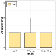
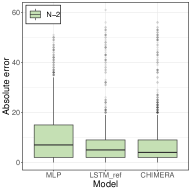
Figure 4: The absolute errors of the numbers of (a) $N-1$ and (b) $N-2$ contingencies given the estimated power flows in the attack-free case.

V-C Impact of False Data Injection Attacks on Contingencies

The performance of the three models against FDIAs is summarized in Table II. Overall, LSTM_ref and CHIMERA achieve better performance compared with the baseline MLP. Regarding the impacts of FDIAs on $N-2$ contingencies, CHIMERA shows higher resilience compared to LSTM_ref.

TABLE II: Average performance of the three models against FDIAs.

Model	MAPE_V	MAPE_$\theta$	MAPE_Total	$\epsilon_{1}^{\mathbf{a}}$	$\epsilon_{2}^{\mathbf{a}}$
MLP	0.27%	0.84%	0.54%	0.35	9.16
LSTMref	0.007%	0.12%	0.06%	0.03	5.75
CHIMERA	0.008%	0.14%	0.07%	0.06	1.70

V-C1 Estimation Accuracy

Denote the estimated states from attacked measurements as $\hat{\mathbf{x}}^{\mathbf{a}}_{t}$. The impact of the attacks on the estimated states is assessed based on the $MAPE\_\theta^{\mathbf{a}}=MAPE(\hat{\bm{\theta}}_{t},\hat{\bm{\theta}}^{\mathbf{a}}_{t})$, $MAPE\_V^{\mathbf{a}}=MAPE(\hat{\mathbf{V}}_{t},\hat{\mathbf{V}}^{\mathbf{a}}_{t})$ and $MAPE\_Total^{\mathbf{a}}=MAPE(\hat{\mathbf{x}}_{t},\hat{\mathbf{x}}^{\mathbf{a}}_{t})$. The results are summarized in Fig. 5. Note that the attacker intends to affect the contingencies while remaining undetected from the state estimation. The results verify the stealthiness of our attack model. We observe that the attacks do not induce large errors to the estimated states: the changes in the estimated states are only 0.54%, 0.06% and 0.07% for the baseline MLP, LSTM_ref, and CHIMERA, respectively. Despite the slight distinctions, we can still conclude that LSTM_ref and CHIMERA are more resilient to FDIAs due to their network architecture and the usage of $L_{static}$.

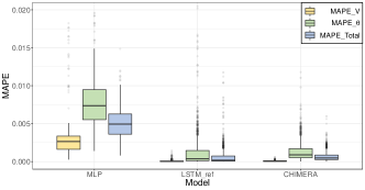
Figure 5: The impact of the attacks on the estimation accuracy.

V-C2 Contingency Analysis Results

Denote the number of the $N-1$ and the $N-2$ contingencies at epoch $t$ given the power flows estimated from the attacked measurements as $\hat{N}^{\mathbf{a}}_{1,t}$ and $\hat{N}^{\mathbf{a}}_{2,t}$. To assess the impacts of the attacks on the contingency analysis, we use the absolute errors between the number of contingencies from estimated power flows before and after attacks, i.e., $\epsilon^{\mathbf{a}}_{1}=|\hat{N}^{\mathbf{a}}_{1,t}-\hat{N}_{1,t}|$ and $\epsilon^{\mathbf{a}}_{2}=|\hat{N}^{\mathbf{a}}_{2,t}-\hat{N}_{2,t}|$, as the performance metrics. The results are presented in Fig. 6. If $\epsilon^{\mathbf{a}}_{1}$ or $\epsilon^{\mathbf{a}}_{2}$ are not equal to 0, an attack is considered successful. Besides, the larger $\epsilon^{\mathbf{a}}_{1}$ or $\epsilon^{\mathbf{a}}_{2}$ are, the larger the impact of the attack is. We observe that the contingency analysis results are sensitive to the accuracy of the estimated states. Although the injected attack vectors have similar magnitudes and only slightly affect the accuracy of the estimated states, the impacts of the attacks on the contingency analysis results from the three models differ a lot. Since no defense is embedded in the baseline MLP, the performance of the baseline MLP is heavily degraded. In the $N-1$ case, 53.50% of $\hat{N}^{\mathbf{a}}_{1}$ are changed ($\epsilon^{\mathbf{a}}_{1}\not=0$) for the baseline MLP, while the percentage of $\hat{N}^{\mathbf{a}}_{1}$ changed for LSTM_ref and CHIMERA are only 31.4% and 22.69%, respectively. The maximum $\epsilon^{\mathbf{a}}_{1}$ is 4 for the baseline MLP, while it is 1 and 2 for LSTM_ref and CHIMERA, respectively. In the $N-2$ case, the average $\epsilon^{\mathbf{a}}_{2,t}$ is 9.16 for the baseline MLP, while the average $\epsilon^{\mathbf{a}}_{2,t}$ is 5.75 for LSTM_ref and 1.70 for CHIMERA. Moreover, the results from LSTM_ref show that using only $L_{static}$ cannot totally defend against FDIAs. On the other hand, because of the usage of the $L_{dynamic}$, the impact of FDIAs on CHIMERA is significantly limited. Specifically, 64.81% of attacks fail to take effect on CHIMERA, i.e., $\epsilon^{\mathbf{a}}_{2}=0$, while the percentages for the baseline MLP and LSTM_ref are only 7.14% and 22.32%, respectively. Moreover, 91.74% of attacks have limited impacts on CHIMERA, i.e., $\epsilon^{\mathbf{a}}_{2}<5$, while for the baseline MLP and LSTM_ref these values are 48.36% and 79.32%, respectively.

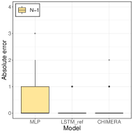
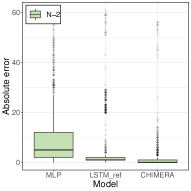
Figure 6: The attack impact on (a) $N-1$ and (b) $N-2$ contingency analysis.

V-D Practical Implications and Applications

In terms of real-world applications, CHIMERA can be implemented at the computing stations of power grid operators and be part of the EMS. For example, it can be deployed as an additional application in the EMS by updating the existing state estimation routines. Thus, CHIMERA does not require or induce any hardware modifications or overhead. The major computation cost of CHIMERA is on the training process. Despite that CHIMERA requires longer training time, it can be trained offline abd it does not induce additional computational overhead during runtime. In fact, the times for CHIMERA and MLP/LSTM_ref to estimate states are of the same order and approximately 0.05ms, which are neglectable and do not violate any real-time requirements [28]. Furthermore, during attacks, significant enhancement has been achieved by CHIMERA in estimating the number of $N-2$ contingencies. For the IEEE 14-bus system, there can be 190 $N-2$ contingencies in total. Through our experiments, we show that in 91.74% attacks, CHIMERA can achieve an estimation accuracy more than 97.4% (i.e., $\epsilon^{\mathbf{a}}_{2}<5$) for $N-2$ contingencies. With such high accuracy, CHIMERA guarantees the normal operation of the power grid during the occurrence of FDIAs.

VI Conclusions

In this paper, we investigate an attack model intending to disturb power systems contingencies through FDIAs. We show that the attack can manipulate contingency analysis accuracy by slightly increasing the state estimation errors. To mitigate the effects, we propose CHIMERA, a hybrid attack-resilient estimator which ensures the accuracy of state estimation and the resulting contingency analysis. CHIMERA leverages the dynamic and static features of the power grid observation model and embeds them into a deep learning model.

References

- [1] Y. Liu, P. Ning, and M. K. Reiter, “False data injection attacks against state estimation in electric power grids,” ACM Transactions on Information and System Security (TISSEC), vol. 14, no. 1, pp. 1–33, 2011.
- [2] A.-Y. Lu and G.-H. Yang, “False data injection attacks against state estimation in the presence of sensor failures,” Information Sciences, vol. 508, pp. 92–104, 2020.
- [3] G. Liang et al., “The 2015 ukraine blackout: Implications for false data injection attacks,” IEEE Transactions on Power Systems, vol. 32, no. 4, pp. 3317–3318, 2016.
- [4] NERC, “Contingency Analysis - basedline,” https://smartgrid.epri.com/UseCases/ContingencyAnalysis-Baseline.pdf.
- [5] J.-W. Kang, I.-Y. Joo, and D.-H. Choi, “False data injection attacks on contingency analysis: Attack strategies and impact assessment,” IEEE Access, vol. 6, pp. 8841–8851, 2018.
- [6] A. S. Musleh, G. Chen, and Z. Y. Dong, “A survey on the detection algorithms for false data injection attacks in smart grids,” IEEE Transactions on Smart Grid, vol. 11, no. 3, pp. 2218–2234, 2019.
- [7] J. Sreenath et al., “A recursive state estimation approach to mitigate false data injection attacks in power systems,” in 2017 IEEE Power & Energy Society General Meeting. IEEE, 2017, pp. 1–5.
- [8] M. N. Kurt, Y. Yılmaz, and X. Wang, “Real-time detection of hybrid and stealthy cyber-attacks in smart grid,” IEEE Transactions on Information Forensics and Security, vol. 14, no. 2, pp. 498–513, 2018.
- [9] Z. Chu, “Unobservable false data injection attacks on power systems,” Ph.D. dissertation, Arizona State University, 2020.
- [10] B. Li et al., “Pama: A proactive approach to mitigate false data injection attacks in smart grids,” in 2018 IEEE Global Communications Conference (GLOBECOM). IEEE, 2018, pp. 1–6.
- [11] A. Sayghe et al., “Survey of machine learning methods for detecting false data injection attacks in power systems,” IET Smart Grid, vol. 3, pp. 581–595, October 2020.
- [12] T. Liu and T. Shu, “Adversarial false data injection attack against nonlinear ac state estimation with ann in smart grid,” in Int’l Conference on Security and Privacy in Communication Systems. Springer, 2019, pp. 365–379.
- [13] A. Sayghe, J. Zhao, and C. Konstantinou, “Evasion attacks with adversarial deep learning against power system state estimation,” in 2020 IEEE Power & Energy Society General Meeting. IEEE, 2020, pp. 1–5.
- [14] O. M. Anubi and C. Konstantinou, “Enhanced resilient state estimation using data-driven auxiliary models,” IEEE Transactions on Industrial Informatics, vol. 16, no. 1, pp. 639–647, 2020.
- [15] L. Wang and Q. Zhou, “Physics-guided deep learning for time-series state estimation against false data injection attacks,” in 2019 North American Power Symposium (NAPS). IEEE, 2019, pp. 1–6.
- [16] C. Konstantinou and M. Maniatakos, “A case study on implementing false data injection attacks against nonlinear state estimation,” in Proceedings of the 2nd ACM workshop on cyber-physical systems security and privacy, 2016, pp. 81–92.
- [17] S.-E. Chien et al., “Automation of contingency analysis for special protection systems in taiwan power system,” in Int’l Conf. on Intelligent Systems Applications to Power Systems. IEEE, 2007, pp. 1–6.
- [18] X. Liu, J. Ospina, and C. Konstantinou, “Deep reinforcement learning for cybersecurity assessment of wind integrated power systems,” IEEE Access, vol. 8, pp. 208 378–208 394, 2020.
- [19] N. Mazzi, B. Zhang, and D. S. Kirschen, “An online optimization algorithm for alleviating contingencies in transmission networks,” IEEE Transactions on Power Systems, vol. 33, no. 5, pp. 5572–5582, 2018.
- [20] X. Liu and C. Konstantinou, “Reinforcement learning for cyber-physical security assessment of power systems,” in 2019 IEEE Milan PowerTech. IEEE, 2019, pp. 1–6.
- [21] I. Zografopoulos et al., “Cyber-physical energy systems security: Threat modeling, risk assessment, resources, metrics, and case studies,” IEEE Access, vol. 9, pp. 29 775–29 818, 2021.
- [22] A. Keliris et al., “Open source intelligence for energy sector cyberattacks,” in Critical Infrastructure Security and Resilience. Springer, 2019, pp. 261–281.
- [23] J. Kim, L. Tong, and R. J. Thomas, “Subspace methods for data attack on state estimation: A data driven approach,” IEEE Transactions on Signal Processing, vol. 63, no. 5, pp. 1102–1114, 2014.
- [24] D. P. Kingma and J. Ba, “Adam: A method for stochastic optimization,” arXiv preprint arXiv:1412.6980, 2014.
- [25] P. Venkatesh, R. Gnanadass, and N. P. Padhy, “Comparison and application of evolutionary programming techniques to combined economic emission dispatch with line flow constraints,” IEEE Transactions on Power systems, vol. 18, no. 2, pp. 688–697, 2003.
- [26] H. Mosbah and M. El-Hawary, “Multilayer artificial neural networks for real time power system state estimation,” in 2015 IEEE Electrical Power and Energy Conference (EPEC). IEEE, 2015, pp. 344–351.
- [27] B. Liu et al., “Recognition and vulnerability analysis of key nodes in power grid based on complex network centrality,” IEEE Trans. on Circuits & Systems II: Express Briefs, vol. 65, no. 3, pp. 346–350, 2017.
- [28] J. Zhao et al., “Power system dynamic state estimation: Motivations, definitions, methodologies, and future work,” IEEE Transactions on Power Systems, vol. 34, no. 4, pp. 3188–3198, 2019.