Anomalous Quantum Information Scrambling for $\mathbb{Z}_{3}$ Parafermion Chains

Abstract

Parafermions are exotic quasiparticles with non-Abelian fractional statistics that could be exploited to realize universal topological quantum computing. Here, we study the scrambling of quantum information in one-dimensional parafermionic chains, with a focus on $\mathbb{Z}_{3}$ parafermions in particular. We use the generalized out-of-time-ordered correlators (OTOCs) as a measure of the information scrambling and introduce an efficient method based on matrix product operators to compute them. With this method, we compute the OTOCs for $\mathbb{Z}_{3}$ parafermions chains up to $200$ sites for the entire early growth region. We find that, in stark contrast to the dynamics of conventional fermions or bosons, the information scrambling light cones for parafermions can be both symmetric and asymmetric, even for inversion-invariant Hamiltonians involving only hopping terms. In addition, we find a deformed light cone structure with a sharp peak at the boundary of the parafermion chains in the topological regime, which gives a unambiguous evidence of the strong zero modes at infinite temperature.

Non-Abelian anyons are elusive quasiparticle excitations emerged from certain topological phases of matter Nayak et al. (2008). They obey non-Abelian braiding statistics and are the building blocks for realizing topological quantum computing Nayak et al. (2008); Kitaev (2003). A prominent example of non-Ableian anyons involves parafermions Clarke et al. (2013); Fendley (2012); Alicea and Fendley (2016); Lindner et al. (2012); Vaezi (2013, 2014); Cheng (2012); Barkeshli and Qi (2014); Stoudenmire et al. (2015); Tsvelik (2014); Klinovaja and Loss (2014); Zhang and Kane (2014); Orth et al. (2015); Alexandradinata et al. (2016); Alavirad et al. (2017); Calzona et al. (2018); Mazza et al. (2018); Hutter and Loss (2016); Alicea and Stern (2015); Chew et al. (2018); Zhuang et al. (2015); Li et al. (2015), which generalize the extensively studied Majornana fermions Kitaev (2001); Fu and Kane (2008); Alicea et al. (2011) and similarly underpin a host of novel phenomena. In particular, braiding of parafermions could supply a richer set of topologically protected operations compared with the Majorana case. Although these operations are still not sufficient to enable computational universality, coupled parafermion arrays in quantum Hall architectures can lead to Fibonacci anyons, which would then harbor universal topological quantum computation Mong et al. (2014). Here, we study the scrambling of quantum information in $\mathbb{Z}_{3}$ parafermion chains, by introducing an efficient algorithm based on matrix product operators (MPOs) to compute the generalized out-of-time-ordered correlators (OTOCs) (see Fig. 1 for an illustration).

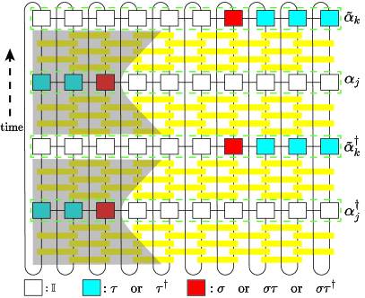
Figure 1: A schematic illustration of the matrix product operator algorithm for computing the out-of-time-ordered correlators for parafermion chains. Here, the computation of $\tilde{F}_{j,k}=\left\langle\alpha_{j}^{\dagger}(t)\tilde{\alpha}_{k}^{\dagger}(0)\alpha_{j}(t)\tilde{\alpha}_{k}(0)\right\rangle$ is shown. The white (blue, red) blocks represent the local identity ($\tau$ or $\tau^{\dagger}$, $\sigma$ or $\sigma\tau$ or $\sigma\tau^{\dagger}$) operators. The yellow blocks represent the Heisenberg time-evolved gates and the shaded regions indicate the induced light cones of $\alpha_{j}(t)$ and $\alpha_{j}^{\dagger}(t)$, respectively. For more details, see the Supplementary Materials Sup .

Information scrambling in quantum many-body systems has attracted tremendous recent attention Hayden and Preskill (2007); Sekino and Susskind (2008); Shenker and Stanford (2014); Hosur et al. (2016); Landsman et al. (2019). It plays an important role in understanding a wide spectrum of elusive phenomena, ranging from the black hole information problem Hayden and Preskill (2007); Sekino and Susskind (2008); Shenker and Stanford (2014); Hosur et al. (2016); Landsman et al. (2019) and quantum chaos Stöckmann (2000) to quantum thermalization and many-body localization Altman (2018); Nandkishore and Huse (2015); Abanin et al. (2019). Whereas black holes are conjectured to be the fastest scramblers in nature Lashkari et al. (2013), the information scrambling in a many-body localized system is much slower Swingle and Chowdhury (2017); Fan et al. (2017); Huang et al. (2017). For conventional bosonic or fermionic systems with translation and inversion symmetries, information scramble in a spatially symmetric way Läuchli and Kollath (2008); Cheneau et al. (2012); Bohrdt et al. (2017). In sharp contrast, it has been shown that asymmetric information scrambling and particle transport could occur for Abelian anyons due to the interplay of anyonic statistics and interactions Liu et al. (2018). In addition, asymmetric butterfly velocities in different directions have also been studied for certain spin Hamiltonians and random unitary circuits Stahl et al. (2018); Zhang and Khemani (2020). Yet, despite these notable progresses, scrambling of information in systems with non-Abelian anyons still remains barely explored. A major challenge faced along this line is that the computation of the OTOC, which is a characteristic measure of information scrambling, is notoriously difficult owing to the exponential growth of the Hilbert dimension involved.

In this paper, we study the scrambling of information in $\mathbb{Z}_{3}$ parafermion chains. We mainly address two questions: (a) How to efficiently access information scrambling for parafermion chains; (b) How information scrambles in parafermion chains? For (a), we propose an efficient algorithm based on MPOs Zwolak and Vidal (2004); Verstraete et al. (2004); Vidal (2007); Schollwöck (2011); Xu and Swingle (2020); White et al. (2018); Hémery et al. (2019) to compute the generalized OTOCs and demonstrate its effectiveness by computing the OTOCs for $\mathbb{Z}_{3}$ parafermion chains as long as $200$ sites for the entire early growth region. For (b), we find that the information scrambling light cones for parafermions can be both symmetric and asymmetric depending on the specific parameter values, even for inversion-invariant Hamiltonians involving only hopping terms. In addition, we find a deformed light cone with a sharp peak at the boundary of the parafermion chains in the topological region, which provides a unambiguous evidence for the existence of strong zero modes at infinite temperature. Our results reveal some crucial aspects of information scrambling for non-Abelian anyons, which would provide a valuable guide for future studies on such exotic quasiparticles in both theory and experiment.

The model Hamiltonian.—We consider the following Hamiltonian for a $\mathbb{Z}_{3}$ parafermion chain Li et al. (2015), which arises naturally from coupled domain walls on the edge of two dimensional (2D) fractionalized topological insulators Lindner et al. (2012); Cheng (2012); Klinovaja et al. (2014); Clarke et al. (2013):

$$H=-t_{1}\sum_{j}e^{i\theta}\alpha_{j}^{\dagger}\alpha_{j+1}+t_{2}\sum_{j}e^{i\phi}\alpha_{j}^{\dagger}\alpha_{j+2}+\text{H.c.},$$ (1)

where $\alpha_{j}$ are parafermion operators obeying $\alpha_{j}^{3}=1$, $\alpha_{j}^{\dagger}=\alpha_{j}^{2}$, and commutation relations $\alpha_{i}\alpha_{j}=\alpha_{j}\alpha_{i}\omega^{\text{sgn}(j-i)},\omega=e^{i{2\pi\over 3}}$, and $t_{1}$, $t_{2}$ control the strength of nearest-neighbor and next-nearest-neighbor hoppings, respectively. Below, we set $t_{1}=1$ as the energy unit. By the generalized Jordan-Wigner transformation Jordan and Wigner (1993) $\alpha_{2j-1}=\left(\prod_{k=1}^{j-1}\tau_{k}\right)\sigma_{j},\alpha_{2j}=\omega\left(\prod_{k=1}^{j-1}\tau_{k}\right)\sigma_{j}\tau_{j}$, the parafermion chain can be mapped to an extended $\mathbb{Z}_{3}$ clock model,

$$H_{c} = -t_{1}\sum_{j}e^{i\theta}\omega\sigma_{j}^{\dagger}\sigma_{j+1}-t_{1}\sum_{j}e^{i\theta}\omega\tau_{j}$$

$$+ t_{2}\sum_{j}(e^{i\phi}\sigma_{j}^{\dagger}\tau_{j+1}\sigma_{j+1}+e^{i\phi}\sigma_{j}^{\dagger}\tau_{j}\sigma_{j+1})+\text{H.c.},$$

where $\sigma_{j}$ and $\tau_{j}$ are generalized spin operators, satisfying $\sigma_{j}^{3}=\tau_{j}^{3}=1$ , $\sigma_{j}\tau_{j}=\omega\tau_{j}\sigma_{j}$ on site and commute with each other off site.

A key quantity to measure information scrambling for parafermion chains is the generalized squared commutator of two local parafermion operators, defined as $C_{j,k}(t)=\left\langle\left[\alpha_{j}(t),\alpha_{k}\right]_{\omega}^{\dagger}\left[\alpha_{j}(t),\alpha_{k}\right]_{\omega}\right\rangle$, which is closely related to the out-of-time-ordered correlator $F_{j,k}(t)=\left\langle\alpha_{j}^{\dagger}(t)\alpha_{k}^{\dagger}(0)\alpha_{j}(t)\alpha_{k}(0)\right\rangle\omega^{\operatorname{sgn}(j-k)}$, through the relation $C_{j,k}=2[1-\operatorname{Re}(F_{j,k})]$. Here the commutator $[\alpha_{j},\alpha_{k}]_{\omega}$ is defined as $[\alpha_{j},\alpha_{k}]_{\omega}=\alpha_{j}\alpha_{k}-\omega^{\operatorname{sgn}(k-j)}\alpha_{k}\alpha_{j}$, and the average $\left\langle\cdot\right\rangle\equiv\text{Tr}(\cdot)/3^{L}$ is measured from the infinite-temperature ensemble. Due to the mathematically equivalence of these two models, one can calculate the physical quantities for the parafermion chains by using the mapped clock models. Yet, local operators in the parafermion model will become highly non-local in the mapped clock model due to the string operators in the generalized Jordan-Wigner transformation. This poses a notable challenge in computing the OTOCs for parafermions. In the following, we introduce an efficient algorithm that could overcome this difficulty.

Algorithm.—Our algorithm is inspired by Xu and Swingle’s MPO approach to computing OTOCs for spin systems in Ref. Xu and Swingle (2020). Suppose we are considering the OTOC for two local Heisenberg operators $W_{0}$ and $V_{r}$ with distance $r\gg 0$, the expansion of $W_{0}(t)$ approximately forms a light cone, which is confined by the Lieb-Robinson bound Lieb and Robinson (1972). The entanglement grow massively inside the light-cone while remain vanishingly small outside. As a result, for computing OTOCs near or outside the light-cone a moderate bond dimension for MPOs suffices. In other words, as long as the local operator $V_{r}$ lies outside the light-cone of $W_{0}(t)$, the calculation of the OTOC using MPO is always efficient and effective. However, for parafermion models, local parafermion operators become highly non-local string operators under the Jordan-Wigner transformation. For instance, we consider the OTOC between $\alpha_{2j+1}$ and $\alpha_{2k+1}$ for parafermions, which is equivalent to calculate the OTOC of two non-local operators $\left(\prod_{n=1}^{j-1}\tau_{n}\right)\sigma_{j}$ and $\left(\prod_{n=1}^{k-1}\tau_{n}\right)\sigma_{k}$ in the $\mathbb{Z}_{3}$ spin model. These two string operators have vanishing distance between them, which renders the direct MPO approach inapplicable.

To overcome this problem, we find that instead of $F_{j,k}$ one can calculate the equivalent quantity $\tilde{F}_{j,k}$ defined as:

$$\tilde{F}_{j,k}(t)=\left\{\begin{aligned} &\left\langle\tilde{\alpha}_{j}^{\dagger}(t)\alpha_{k}^{\dagger}(0)\tilde{\alpha}_{j}(t)\alpha_{k}(0)\right\rangle,j\geq k\\ &\left\langle\alpha_{j}^{\dagger}(t)\tilde{\alpha}_{k}^{\dagger}(0)\alpha_{j}(t)\tilde{\alpha}_{k}(0)\right\rangle,j<k\end{aligned}\right.,$$ (3)

where $\tilde{\alpha}_{j}(t)\equiv P^{\dagger}\alpha_{j}(t)$ with $P=\prod_{j}\tau_{j}$ being the parity operator satisfying $P^{3}=1$ and $[H,P]=0$. Mathematically, we can prove that $F_{j,k}=\tilde{F}_{j,k}$ Sup . Now, the left-string operator $\alpha_{2k+1}=\left(\prod_{n<k}\tau_{n}\right)\sigma_{k+1}$ changes into the right-string operator $\tilde{\alpha}_{2k+1}=\left(\prod_{n\geq k}\tau^{\dagger}_{n}\right)\sigma_{k+1}$, which restores the distance between two operators in computing OTOCs via the MPO approach. Our algorithm is pictorially illustrated in Fig. 1 with more details given in the Supplementary Materials Sup .

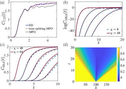
Figure 2: (a) A comparison between results from the MPO algorithms and exact diagonalization (ED). Here, the bond dimension $\chi=48$ is used. (b) The results of $C_{j,k}$ in the early-growth regime by the MPO algorithm with $j=100$ and $k=80,60,40,20$. (c) The results of $C_{j,k}$ for the later-time regime with $j=60$ and $k=50,40,30,20,10$. (d) The light-cone structure of the OTOC $\text{Re}[F_{j,k}(t)]$ is plotted with $j=100$. We fix $\theta=\phi=0$ and other parameters are chosen as: $t_{2}=1$ for (b) and $t_{2}=0.5$ for (a), (c) and (d); $L=14,200,120,200$ for (a), (b), (c), and (d), respectively.

For the time-evolved MPOs in the early growth regime (before the wavefront reaches the left side of the right-string operator $\tilde{\alpha}_{k}$ ) , the truncation error is bounded owning to the entanglement lightcone structure and wiped off by the average over the infinite-temperature ensemble. To access the OTOC for a longer time, we may use the time-splitting MPO method: $\tilde{F}_{j,k}(t)=\tilde{F}_{j,k}^{\text{late}}(t)=\langle\alpha_{j}^{\dagger}(t/2)\tilde{\alpha}_{k}^{\dagger}(-t/2)\alpha_{j}(t/2)\tilde{\alpha}_{k}(-t/2)\rangle$ for $j<k$, where we evolve both local parafermion operators in forward and backward directions. With this method, we can capture the information scrambling in parafermion chains in both early-time and later-time regimes.

Light-cone structure.—We now study the scrambling of information for parafermion chains. We first benchmark the effectiveness and accuracy of our algorithm. In Fig.2(a), we compare the MPO results with that from the exact diagonalization (ED) for a short parafermion chain with $L=14$. We find that with a moderate bond dimension ($\chi=48$), the MPO method without time-splitting works excellently for the entire early-growth regime, whereas for later times it becomes inaccurate due to the growth of entanglement. In contrast, the time-splitting MPO method works for both the early-time and later-time regimes with relative error smaller than $1\%$. In the following, we will use the the time-splitting MPO method with a small Trotter step $dt=0.002$ by default.

Then we compute the OTOCs for much longer parafermion chains, which are far beyond the capability of the ED method. In Fig.2(b), we plot the result of $C_{j,k}$ in the early-growth regime with the system size $L=200$. It is clear that the curves for bond dimension $\chi=8$ match almost precisely with that for $\chi=48$, indicating that a small bond dimension is sufficient for computing OTOCs in the early-growth regime. For the later-growth regime, we also calculate $C_{j,k}$ with different bond dimensions for a parafermion chain with system size $L=120$, and our result is shown in Fig.2(c). We find that the curves for $\chi=48$ match that for $\chi=64$ in the regime $C_{j,k}<0.4$, but after that deviations will show up owning to the growth of entanglement.

The above discuss have clearly demonstrated the effectiveness of our MPO method in computing OTOCs for parafermion chains in the entire early-growth regime. Truncation to small bond dimension only results in errors after the wavefront, and the scrambling of information ahead of and up to the wavefront can be captured accurately with our approach. Now, we discuss the anomalous quantum information scrambling for parafermion chains. First, we note that the model in Eq. (1) is integrable when $\theta=\phi=0$ and $t_{2}=0$, where the OTOCs map out a symmetric light cone Sup , similar to the cases for conventional fermions or bosons. However, as shown in Fig. 2(d), when we turn on the next-nearest-neighbor hoppings ($t_{2}\neq 0$) the light cone will become asymmetric, implying that the information propagation is asymmetric for the left and right directions. We stress that from the perspective of parafermions, the Hamiltonian is fully left-right symmetric when $\theta=\phi=0$. The dynamic broken of the left-right symmetry is a reflection of anyonic statistics of the parafermions.

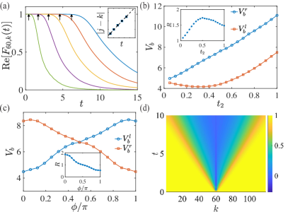
Figure 3: (a) The dynamics of the OTOCs for a parafermion chain with length $L=120$, which characterizes the quantum information spreading from the middle of the chain ($j=60$) to the left $k=50,40,30,20,10$. The black arrows mark the positions where the OTOCs drop $1\%$ of their initial values, which are used to extract the butterfly velocity through linear fit as shown in the inset. Here, the bond dimension $\chi=32$ is used and other parameters are chosen as $\theta=\phi=0$ and $t_{2}=0.9$. (b) The extracted left ($V_{b}^{l}$) and right ($V_{b}^{r}$) butterfly velocities as a function of $t_{2}$. The inset shows the ratio $R=V_{b}^{r}/V_{b}^{l}$ versus $t_{2}$. (c) Dependence of $V_{b}^{l}$ and $V_{b}^{r}$ on $\phi$ when $\theta=\pi/6$ and $t_{2}=0.5$, with the inset showing the corresponding ratio. (d) The symmetric light-cone structure of the OTOCs with $\theta=\pi/6$, $\phi=\pi/2$, and $t_{2}=0.5$.

A more precise way to quantify the asymmetry of the information spreading is to utilize the butterfly velocity $V_{b}^{l}$ ($V_{b}^{r}$) for the left (right) directions. We defined the butterfly velocity $V_{b}^{l/r}$ by the boundary of the space-time region where $\text{Re}(F_{j,k})$ drops by at least $1\%$ of its initial values, as marked by arrows in Fig.3(a). The linear fits of butterfly velocities $V_{b}^{l,r}$ with varying $t_{2}$ are shown in Fig. 3(b), from which it is clear that $V_{b}^{r}>V_{b}^{l}$ for the whole region $t_{2}>0$, indicating that information scrambles faster to the right direction. In addition, it is also interesting to note that $V_{b}^{r}$ increases monotonically as $t_{2}$ increases. Whereas, the dependence of $V_{b}^{l}$ on $t_{2}$ is non-monotonic: it decreases at first and then increases. A maximum deviation of $V_{b}^{l}$ from $V_{b}^{r}$ occurs around $t_{2}=0.5$. In Fig.3(c), we plot $V_{b}^{l,r}$ with varying $\phi$ and fixed $\theta=\pi/6$. Interestingly, $V_{b}^{l,r}$ have a crucial dependence on $\phi$: one can make information scrambles faster to the right (or left) direction by tuning $\phi$. When $\phi=\pi/2$, we find that $V_{b}^{l}=V_{b}^{r}$ and the light cone is fully symmetric, as shown in Fig. .3(d).

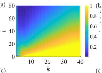
Figure 4: The light-cone structures of the OTOCs $\text{Re}[F_{1,k}(t)]$ for the parafermion chain model defined in Eq. (4), with $\varphi=-\pi/6$, $J_{1}=1$, $L=40$, and $J_{2}=0.4,0.5,0.6$ respectively in (a), (b), and (c). The bond dimension is $\chi=48$. (d) The results of $C_{1,L}$ with varying $J_{2}=0.1,0.2,\cdots,1.0$ from right to left. The curves for $\chi=32$ matches that of $\chi=64$ precisely, indicating a negligible truncation error for the MPO algorithm in computing these OTOCs.

Symmetry analysis.— In the Fig.3(c), we find that $V^{l}_{b}(\phi)=V^{r}_{b}(\pi-\phi)$ and the preferred information scrambling direction can be reversed by sending $\phi\rightarrow\pi-\phi$. Here, we show that this observation can be understood from the symmetry analysis of the Hamiltonian. In fact, one can use two successive transformations, $(\sigma\rightarrow\sigma^{\dagger},\tau\rightarrow\tau^{\dagger})$ and $(\tau\rightarrow\omega^{-1}\tau$, $\sigma_{2j}\rightarrow\omega^{-1}\sigma_{2j}$, $\sigma_{2j+1}\rightarrow\sigma_{2j+1})$, to obtain $H_{c}(\theta=\pi/6,\phi)\rightarrow-H_{c}(\theta=\pi/6,\pi-\phi)$ and $\alpha_{j}^{\phi}(t)\rightarrow\alpha_{j}^{(\pi-\phi)\dagger}(-t)$, where the $\alpha_{j}^{\phi}(t)$ donates the evolution of a parafermion $\alpha_{j}(0)$ under the Hamiltonian $H_{c}(\theta=\pi/6,\phi)$ Sup . Noting in addition that $\langle\alpha_{j}^{\dagger}(t)\alpha_{k}^{\dagger}(0)\alpha_{j}(t)\alpha_{k}(0)\rangle=\langle\alpha_{j}^{\dagger}(0)\alpha_{k}^{\dagger}(-t)\alpha_{j}(0)\alpha_{k}(-t)\rangle$, we thus obtain $C_{j,k}^{\phi}(t)=C_{k,j}^{\pi-\phi}(t)$, which explains the inversion symmetry between curves of $V^{l}_{b}$ and $V^{r}_{b}$. Particularly, when $\phi=\pi/2$ we have $C_{j,k}^{\pi/2}(t)=C_{k,j}^{\pi/2}(t)$, giving rise to the fully symmetric light cone shown in Fig.3(d).

Scrambling for strong zero modes.—Strong zero modes lead to degeneracies across the entire spectrum and thus may offer potential advantages in building fault-tolerant qubits that works at high temperatures. With the introduced MPO algorithm, we are able to study information scrambling for strong zero modes at even infinite temperature. To this end, we consider the following parafermion chain model with alternating nearest-neighbour couplings Jermyn et al. (2014); Fendley (2012):

$$H=-J_{1}\sum_{j}e^{i\varphi}\alpha_{2j}^{\dagger}\alpha_{2j+1}-J_{2}\sum_{j}\alpha_{2j-1}^{\dagger}\alpha_{2j}+\text{H.c.}.$$ (4)

The stability of the zero modes in this model has been discussed and the regime where the strong zero modes may exist has also been estimated based on perturbation analysis and density matrix renormalization group algorithm near the ground states Jermyn et al. (2014). In the limit $J_{2}\rightarrow 0$, the outermost parafermion operators drop out from the Hamiltonian (similar as in the Kitaev chain for Majoranas Kitaev (2001)) and represent localized zero modes that guarantee a threefold degeneracy for the whole spectrum. However, unlike the Majorana case for this $\mathbb{Z}_{3}$ parafermion chain there are strong evidences that localized zero modes disappear completely upon introducing arbitrarily small $J_{2}$ when $\varphi=0$, which is rather counterintuitive given that the system is in a gapped topological phase. Whereas, for nonzero $\varphi$ stable localized zero modes seems to survive small nonzero $J_{2}$ indeed Jermyn et al. (2014); Fendley (2012).

For our purpose, we compute the OTOC of two parafermion operators at the open ends $F_{1,L}(t)$ and our results are shown in Fig. 4. Here, we choose $\varphi=-\pi/6$ since at this point the zero modes are suspected to be the most robust Jermyn et al. (2014); Moran et al. (2017). In Fig.4(a-c), we plot $\text{Re}[F_{1,k}(t)]$ with $L=40$, $J_{1}=1$ and varying $J_{2}$. From Fig.4(a), we see a sharp peak at the boundary of the light cone for $J_{2}=0.4$, indicating a drastically lengthened scrambling time for the zero modes localized at the ends of the chain. Given that the our OTOC is calculated at infinite temperature, this sharp peak is a clear-cut evidence of the existence of strong zero modes at the ends of the parafermion chain for nonzero $J_{2}$. When $J_{2}$ increases, this peak diminishes and nearly disappears when $J_{2}=0.6$, as shown in Fig. 4(b,c). This implies the transition point is in the regime $J_{2}=0.4\sim 0.6$, which is consistent with the perturbative analysis in Ref. Jermyn et al. (2014). To see it more clearly, we calculate the $C_{1,40}$ for increasing $J_{2}$ in Fig.4(d). As we can see, for a fixed time window $t<100$, the squared commutator $C_{1,L}$ increases rapidly and saturate to its maximum value very soon for $J_{2}\geq 0.6$. While for $J_{2}<0.6$ , it increases much slower, indicating the presence of strong zero modes as well.

Discussion and conclusion.— A number of protocols for measuring OTOCs in various systems have been proposed Swingle et al. (2016); Zhu et al. (2016); Yao et al. (2016); Halpern (2017); Halpern et al. (2018); Campisi and Goold (2017); Yoshida and Kitaev (2017). Indeed, recently experimental measurement of OTOCs has been demonstrated with trapped ions Gärttner et al. (2017) and nuclear magnetic resonance quantum simulators Wei et al. (2018); Li et al. (2017). For $\mathbb{Z}_{3}$ parafermions, different blueprints for their experimental realization have also been introduced in a variety of systems, ranging from lattice defects in fractional Chern insulators Vaezi (2014) and fractionalized topological insulators/superconductors Klinovaja et al. (2014); Cheng (2012) to quantum Hall bilayers Barkeshli and Qi (2014); Peterson et al. (2015) and bosonic cold atoms Maghrebi et al. (2015). Yet, to the best of our knowledge, no experimental proposal of measuring OTOCs for $\mathbb{Z}_{3}$ parafermions has been introduced hitherto. In the future, it would be interesting to study how OTOCs for parafermion chains can be measured in experiment and consequently observe the anomalous information scrambling predicted in this paper.

In summary, we have introduced a low-cost MPO algorithm to calculate the OTOCs for parafermion chains, which can capture the scrambling of quantum information in the entire early-growth regime with modest bond dimension. With this powerful algorithm, we have explored the anomalous information dynamics for $\mathbb{Z}_{3}$ parafermion chains up to a system size far beyond the capability of previous numerical approaches. We found that information can scramble both symmetrically and asymmetrically for parafermion chains, even for inversion-invariant Hamiltonians involving merely hopping terms. In addition, we found a deformed light cone structure with a sharp peak at the boundary, which offers a unambiguous evidence of the strong zero modes at infinite temperature. Although we have only focused on $\mathbb{Z}_{3}$ parafermions, our introduced algorithm applies to the general $\mathbb{Z}_{n}$ parafermions and Abelian anyons (such as the anyon-Hubbard model) as well. Our results not only provide a powerful method for accessing quantum information scrambling in systems with exotic quasiparticles, but also uncover the peculiar information dynamics for parafermions which would benefit future studies in both theory and experiment.

We acknowledge helpful discussions with Fang-Li Liu and Sheng-Long Xu. This work is supported by the start-up fund from Tsinghua University (Grant. No. 53330300320), the National Natural Science Foundation of China (Grant. No. 12075128), and the Shanghai Qi Zhi Institute.

Anomalous Quantum Information Scrambling for $\mathbb{Z}_{3}$ Parafermion Chains

S.I The MPO algorithm

In the main text, we have given a brief introduction to the MPO algorithm for calculating the OTOCs in parafermion chains. Here we generalize this method to some other models which consist of on-site symmetries and give more details of the MPO algorithm.

S.I.1 General models

Our algorithm is generally applicable for Hamiltonians which obey certain on-site symmetry, that is

$$S=\otimes_{n}u_{n}.$$ (S1)

Here, $u_{n}$ is an on-site operator on the $n$ site and $[S,H]=0$. A general OTOC can be written as

$$F_{ij}=\langle W_{i}^{\dagger}(t)V_{j}^{\dagger}W_{i}(t)V_{j}\rangle,$$ (S2)

where $W,V$ are unitary operators. By inserting the identity operator $\mathbb{I}=SS^{\dagger}$ into the OTOC, we obtain

$$F_{ij}=\langle e^{iHt}W_{i}^{\dagger}e^{iHt}V_{j}^{\dagger}SS^{\dagger}e^{iHt}SS^{\dagger}W_{i}SS^{\dagger}e^{-iHt}SS^{\dagger}V_{j}\rangle.$$ (S3)

If we add the condition $S^{\dagger}W_{i}S\sim W_{i}$ ($\sim$ means equal up to a constant), accompanying with $S^{\dagger}e^{iHt}S=e^{iHt}$, the OTOC $F_{ij}$ reduces to

$$F_{ij}\sim\langle W_{i}^{\dagger}(t)(V_{j}^{\dagger}S)W_{i}(t)(S^{\dagger}V_{j})\rangle.$$ (S4)

Then the OTOC between $W_{i}$ and $V_{j}$ is equivalent to the OTOC between $W_{i}$ and $S^{\dagger}V_{j}$.

Taking anyon-Hubbard model for example. The anyon-Hubbard model can be written as

$$H_{A}=-J\sum_{j=1}\left(a_{j}^{\dagger}a_{j+1}+\mathrm{H.c.}\right)+\frac{U}{2}\sum_{j=1}n_{j}(n_{j}-1),$$ (S5)

and the OTOC is defined as

$$F_{jk}^{A}(t)=\Braket{a_{j}^{\dagger}(t)a_{k}^{\dagger}(0)a^{\phantom{\dagger}}_{j}(t)a^{\phantom{\dagger}}_{k}(0)}e^{i\theta\operatorname{sgn}(j-k)}.$$ (S6)

The Hamiltonian has symmetry $S_{A}=e^{-i\theta\sum_{j}a_{j}^{\dagger}a_{j}}$. By utilizing the same transformation as Eq. S3 , $F_{jk}^{A}(t)$ is transformed to

$$F_{jk}^{A}(t)=\Braket{a_{j}^{\dagger}(t)\left(a_{k}^{\dagger}(0)S_{A}\right)a^{\phantom{\dagger}}_{j}(t)\left(S_{A}^{\dagger}a^{\phantom{\dagger}}_{k}(0)\right)}.$$ (S7)

Since $a_{k}=b_{k}e^{-i\theta\sum_{j<k}a_{j}^{\dagger}a_{j}}$ is a left string operator, $\left(S_{A}^{\dagger}a_{k}(0)\right)$ become a right string operator. Here, $b_{k}$ is the Boson annihilation operator.

In the next part, we calculate the OTOCs in parafermion chains with $L=20$ as an illustrating example.

S.I.2 The details of the MPO algorithm

In the main text, we have introduced the algorithm from entanglement points of view, especially emphasized the importance of the distance between two local operators in the calculation of OTOCs. In this section, we give more details about the reason why this condition is essential for the MPO method to work well in the early-growth regime. However, this condition is not sufficient, as we would mention below, the calculation of OTOC with infinite-temperature ensembles is also important.

Without loss of generality, we consider the calculation of the OTOCs

$$F_{j,k}(t)=\left\langle\alpha_{j}^{\dagger}(t)\alpha_{k}^{\dagger}(0)\alpha_{j}(t)\alpha_{k}(0)\right\rangle\omega^{\operatorname{sgn}(j-k)},$$ (S8)

in a 20-sites parafermion chain, which can be mapped to a 10-sites $\mathbb{Z}_{3}$ spin chain. Next, we take $j=5,k=13$ for example. The local parafermion operators can be written as

$$\alpha_{5} =\tau_{1}\tau_{2}\sigma_{3},$$ (S9)

$$\alpha_{13} =\tau_{1}\tau_{2}\tau_{3}\tau_{4}\tau_{5}\tau_{6}\sigma_{7},$$

and the general MPO calculation of $F_{j,k}(t)$ is illustrated in Fig.S1. We use blue(red) blocks to represent the operator $\tau$($\sigma$) and use white blocks to represent the identity operator. The MPO evolution is based on time-evolving block decimation (TEBD) method Vidal (2004), which is represented by yellow blocks. The trace operation corresponds to contracting all the physical indices from top to bottom. The grey regions correspond to the induced operator light-cone expansion. However, this direct MPO calculation could only capture the early time regime of OTOC growth, due to the rapid growth of entanglement which induces huge truncation errors.

In order to get rid of these truncation errors, we calculate the modified but mathematically equivalent quantity obtained by inserting the parity operator $P=\prod_{j}\tau_{j}$ inside the OTOC:

$$F_{5,13}(t) =\left\langle\alpha_{5}^{\dagger}(t)\alpha_{13}^{\dagger}(0)PP^{\dagger}\alpha_{5}(t)PP^{\dagger}\alpha_{13}(0)\right\rangle\omega^{2}$$ (S10)

$$=\left\langle\alpha_{5}^{\dagger}(t)\left(\alpha_{13}^{\dagger}(0)P\right)\alpha_{5}(t)\left(P^{\dagger}\alpha_{13}(0)\right)\right\rangle$$

$$=\left\langle\alpha_{5}^{\dagger}(t)\tilde{\alpha}_{13}^{\dagger}(0)\alpha_{5}(t)\tilde{\alpha}_{13}(0)\right\rangle\equiv\tilde{F}_{5,13}(t),$$

where the operator $\tilde{\alpha}_{13}=\tau_{7}\sigma_{7}\tau_{8}\tau_{9}\tau_{10}$ becomes right string form, as illustrated in Fig. 1 in the main text.

The MPO calculation of $\tilde{F}_{5,13}(t)$ could be simplified using the product form of $\tilde{\alpha}_{13}$, see Fig. S2(a). Here, we have replaced $\alpha_{5}^{\dagger}(t)$ with $\mathrm{W}(t)$ in MPO form, and $W_{i}(t)$ are tensors of $W(t)$ at site $i$. Then, taking advantage of the left canonical condition of MPO

$$\sum_{\sigma_{l},\sigma_{l^{\prime}}}W_{i}^{\sigma_{l},\sigma_{l^{\prime}}\dagger}W_{i}^{\sigma_{l},\sigma_{l^{\prime}}}=\mathbb{I},$$ (S11)

which is shown in graphical representation in Fig.S2(b), the MPO of OTOC reduces to the structure of Fig.S2(c).

Now we see that the calculation of the OTOC is only related to the contraction of the tensor right to the site $k$. Therefore , as long as the truncation error is small for these local MPO tensors, the MPO algorithm is effective. In fact, as the truncation error is confined by the light-cone in the early-growth regime, our method is efficient. It is worth mentioning that the left canonical condition entails the trace operation, which means that the OTOC computed is averaged at infinite-temperature.

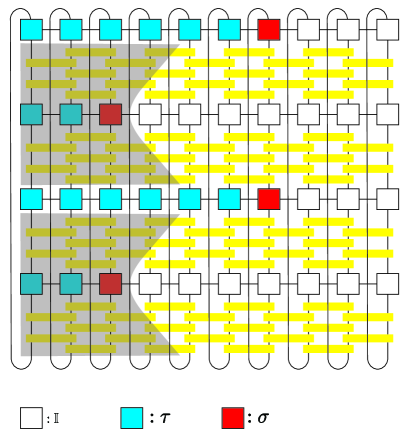
Figure S1: Graphical representation for the OTOC $F_{j,k}$($j<k$) in the natural tensor network form, in contrast to the modified $\tilde{F}_{j,k}$ in Fig.1 in the main text. Here, we choose the parameter $j=5,k=13$.

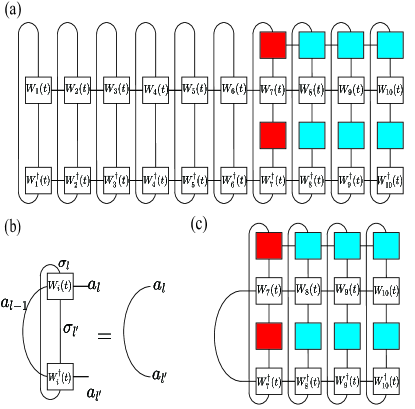
Figure S2: (a) Reduction of the tensor network from the Fig.1 in the main text. The $\alpha_{5}(t)$ is replaced by MPO $\mathrm{W}(t)$. (b) Left canonical condition of MPO tensors is illustrated in diagram, $\sigma_{l}$ and $\sigma_{l^{\prime}}$ are physical indices and $a_{l},a_{l^{\prime}},a_{l-1}$ are vurtual indices. (c) Simplified MPO representation of OTOC.

S.II Hamiltonian and dynamical symmetries

In the main text, we have mentioned the relevant symmetries for the OTOC dynamics. Here, we give the detailed derivation for them.

S.II.1 Hamiltonian symmetry

To discuss the symmetry in an explicit way, we give the representation of $\sigma_{j}$ and $\tau_{j}$ in the matrix form:

$$\sigma=\left(\begin{array}[]{lll}0&1&0\\ 0&0&1\\ 1&0&0\end{array}\right),\quad\tau=\left(\begin{array}[]{ccc}1&0&0\\ 0&\omega&0\\ 0&0&\omega^{2}\end{array}\right),\quad\omega=e^{2\pi i/3}$$ (S12)

First, we consider the symmetry of the mapped clock Hamiltonian and define the inversion transformation $\mathcal{I}$ as:

$$\mathcal{I}:\sigma_{j}\rightarrow\sigma_{N-j+1},\ \tau_{j}\rightarrow\tau_{N-j+1}.$$ (S13)

Then, we introduce the following time-reversal anti-unitary transformation $\mathcal{T}$ as

$$\mathcal{T}:\sigma_{j}\rightarrow\sigma_{j},\ \tau_{j}\rightarrow\tau^{\dagger}_{j}.$$ (S14)

The composition $\mathcal{T}\circ\mathcal{I}$ defines a new operation which leave the Hamiltonian invariant. This transformation changes the Hamiltonian $H_{c}$ as

$$\tilde{H}_{c}= -t_{1}\sum_{j=1}^{N-1}e^{-i\theta}\omega^{2}\sigma_{N+1-j}^{\dagger}\sigma_{N-j}-t_{1}\sum_{j=1}^{N}e^{-i\theta}\omega^{2}\tau^{\dagger}_{N+1-j}\qquad$$ (S15)

$$+t_{2}\sum_{j=1}^{N-1}e^{-i\phi}\sigma_{N+1-j}^{\dagger}\tau^{\dagger}_{N-j}\sigma_{N-j}$$

$$+t_{2}\sum_{j=1}^{N-1}e^{-i\phi}\sigma_{N+1-j}^{\dagger}\tau^{\dagger}_{N+1-j}\sigma_{N-j}+\mathrm{H.c.}$$

From the parafermion perspective, this transformation $\mathcal{T}\circ\mathcal{I}$ inverses the parafermion sites as

$$\mathcal{T}\circ\mathcal{I}:\alpha_{j}\rightarrow\tilde{\alpha}_{-j}\equiv P\alpha_{-j},$$ (S16)

and the anti-unitary operation preserve the commutation relation $\alpha_{i}\alpha_{j}=\alpha_{j}\alpha_{i}\omega^{\text{sgn}(j-i)}$. The detailed transformation of $\alpha_{j}$ by $\mathcal{T}\circ\mathcal{I}$ is:

$$\alpha_{2j-1} = \left(\prod_{k=1}^{j-1}\tau_{k}\right)\sigma_{j}$$ (S17)

$$\rightarrow \tilde{\alpha}_{2N+2-2j}=\left(\prod_{k=N}^{N+2-j}\tau^{\dagger}_{k}\right)\sigma_{N+1-j},$$ (S18)

$$\alpha_{2j} = \omega^{2}\left(\prod_{k=1}^{j-1}\tau_{k}\right)\sigma_{j}$$ (S19)

$$\rightarrow \tilde{\alpha}_{2N+1-2j}=\omega\left(\prod_{k=N}^{N+1-j}\tau^{\dagger}_{k}\right)\sigma_{N+1-j},$$ (S20)

which leaves the commutation relation invariant

$$\tilde{\alpha}_{j}^{3}=1,\ \tilde{\alpha}_{j}^{\dagger}=\tilde{\alpha}_{j}^{2},\ \tilde{\alpha}_{i}\tilde{\alpha}_{j}=\tilde{\alpha}_{j}\tilde{\alpha}_{i}\omega^{\text{sgn}(j-i)}.$$ (S21)

However, this symmetry does not guarantee the symmetry of the OTOC dynamics.

S.II.2 Dynamical symmetry

In the main text, the special line $\theta=\pi/6,\phi=\pi/2$ exhibits OTOC dynamical symmetry with regard to the parafermion chain model. We consider the effect of two successive transformations on the OTOC. Initially, we assume the Hamiltonian is $H_{c}(\theta=\pi/6,\phi)$. We define a transformation $\mathcal{U}$ as

$$\mathcal{U}:\sigma\rightarrow\sigma^{\dagger},\tau\rightarrow\tau^{\dagger},$$ (S22)

where $\mathcal{U}$ is a unitary transformation with matrix representation

$$U=\left(\begin{array}[]{lll}1&0&0\\ 0&0&1\\ 0&1&0\end{array}\right),$$ (S23)

and the transformation maps the Hamiltonian as

$$H_{c}(\theta=\pi/6,\phi)\rightarrow H_{c}(\theta=-\pi/6,2\pi/3-\phi).$$ (S24)

In the second transformation, we redefine

$$\tau\rightarrow\omega^{-1}\tau,\quad\sigma_{2j}\rightarrow\omega^{-1}\sigma_{2j},\quad\sigma_{2j+1}\rightarrow\sigma_{2j+1},$$ (S25)

the Hamiltonian changes as

$$H_{c}(\theta=-\pi/6,2\pi/3-\phi)\rightarrow-H_{c}(\theta=\pi/6,\pi-\phi).$$ (S26)

Then under the two successive transformations, the Hamiltonian changes as

$$H_{c}(\theta=\pi/6,\phi)\rightarrow-H_{c}(\theta=\pi/6,\pi-\phi).$$ (S27)

Whereas the parafermion operator changes as

$$\alpha_{j}^{\phi}(t)\rightarrow\alpha_{j}^{(\pi-\phi)\dagger}(-t),$$ (S28)

where $\alpha_{j}^{\phi}(t)$ is defined by

$$\alpha_{j}^{\phi}(t)\equiv e^{iH_{c}(\theta=\pi/6,\phi)}\alpha_{j}e^{-iH_{c}(\theta=\pi/6,\phi)}.$$ (S29)

Then $F_{j,k}=\langle\alpha_{j}^{\phi\dagger}(t)\alpha_{k}^{\dagger}(0)\alpha^{\phi}_{j}(t)\alpha_{k}(0)\rangle\omega^{\operatorname{sgn}(j-k)}$ changes to

$$\langle\alpha_{j}^{\pi-\phi}(-t)\alpha_{k}(0)\alpha_{j}^{(\pi-\phi)\dagger}(-t)\alpha_{k}^{\dagger}(0)\rangle\omega^{\operatorname{sgn}(j-k)}.$$ (S30)

Using the identity

$$\langle\alpha_{j}^{\dagger}(t)\alpha_{k}^{\dagger}(0)\alpha_{j}(t)\alpha_{k}(0)\rangle=\langle\alpha_{j}^{\dagger}(0)\alpha_{k}^{\dagger}(-t)\alpha_{j}(0)\alpha_{k}(-t)\rangle,$$ (S31)

as well as the property of trace operation, the OTOC becomes

$$\langle\alpha_{j}^{\dagger}(0)\alpha_{k}^{(\pi-\phi)\dagger}(t)\alpha_{j}(0)\alpha^{\pi-\phi}_{k}(t)\rangle\omega^{\operatorname{sgn}(j-k)}\equiv F_{k,j}^{\dagger}.$$ (S32)

Finally, taking advantage of $C_{i,j}=2(1-\text{Re}(F_{i,j}))$, we obtain

$$C^{\phi}_{j,k}(t)\rightarrow C^{\pi-\phi}_{k,j}(t),$$ (S33)

which explains the symmetry of dynamics in the main text.

S.III Level statistics

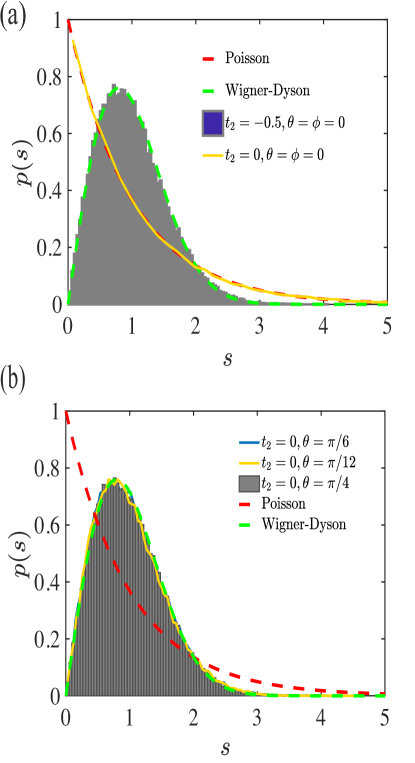
Figure S3: Level space distribution of the spectra for model Eq.1 in the main text with chain length $L=12$. The spectra are restricted in parity $P=0$ subspace and the results for $P=1$ and $P=2$ are similar. Dashed curves are $P(s)=e^{-s}$(red) and $P(s)=\frac{\pi}{2}s\mathrm{e}^{-\frac{\pi}{4}s^{2}}$(green), typical for integrable or quantum chaotic systems.

To check whether a many-body Hamiltonian in a certain regime is integrable or quantum chaotic, we calculate the level space distribution of the spectra, which is a strong indicator for quantum chaos Haake (1991).

In Fig.S3(a-b), we show the level space distribution for the Hamiltonian in Eq. (1) in the main text for different parameter regimes. In the special point, where the next-nearest-neighbor interaction is turned off and $\theta=0$, the model is integrable, which is illustated in Fig. S3(a). The levels show no repulsion and the probability distribution of spacings is approximately given by $P(s)=e^{-s}$. Despite this point, as we increase the next-nearest-neighbor interaction, see Fig. S3(a), or add a no-zero chiral phase, see Fig. S3(b), we find a level repulsion and the statistics follows the Wigner-Dyson distribution. The level spacing distribution has the following shape, $P(s)=\frac{\pi}{2}s\mathrm{e}^{-\frac{\pi}{4}s^{2}}$, which indicates the nonintegrablility of the model.

S.IV more numerical results

In this section, we give more numerical results on the OTOC calculation. We first consider the special case, when the angle $\theta=\phi=0$. We can clearly see from Fig. S4(a) that the information spreading asymmetric between two directions when the next-nearest-neighbor coupling is turned off. The information scrambles much faster to the right than to the left and it seems that there does not exist a clear wavefront in the left-hand side. This is due to the integrability of the model with only nearest-neighbor couplings at the point $\theta=\phi=0$. In Fig. S4(c), we plot the OTOC in time-space with parameter $\theta=\pi/6$, $\phi=\pi/2$, $t_{2}=0$, and find the light-cone structure is indeed symmetric, which is consistent with the symmetry analysis results in S.II. In Fig. S4(b), (d), we calculate the OTOC both in the early and later growth regime and set $j<k$, which are in parallel with the results $j>k$ in the Fig. 2 in the main text. These results indicate that the scrambling can be well captured by the MPO algorithm in both directions with modest bond dimension.

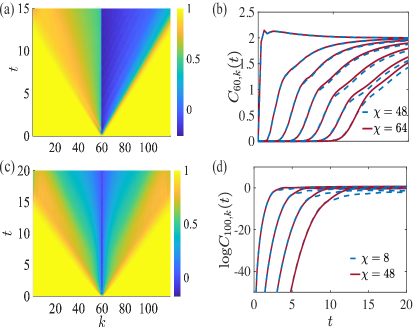
Figure S4: OTOC growth $\text{Re}(F_{j,k})$ are obtained within MPO approach for differen angles $\theta$, $\phi$ in (a),(c) and squared commutators $C_{j,k}$ are plotted in late and early-growth regime in (b),(d). The light-cone structure of OTOC is ploted in (a) with parameters $\theta=\phi=0$, $t_{2}=0$ and $\theta=\pi/6$, $\phi=\pi/2$, $t_{2}=0$ in (c). In both figures, the color maps are interpolated to better illustrate the light-cone structure. The late-growth regime of the squared commutator $C_{j,k}$ are ploted in (b) with parameters $\theta=0$, $\phi=0$, $t_{2}=0.5$,$j=60$ for varying $k=60,70,80,90,100,110$ and the early-growth regime of the squared commutator $C_{j,k}$ are plotted in (d) with parameters $\theta=0$, $\phi=0$, $t_{2}=1$,$j=100$ for varying $k=120,140,160,180$.

S.V The OTOC in the topological regime

The OTOC between parafermions at the two open ends can be written as

$$F_{1,L}=\frac{1}{3^{L/2}}\operatorname{Tr}\left(\alpha_{1}^{\dagger}(t)\alpha_{L}^{\dagger}\alpha_{1}(t)\alpha_{L}\right)\omega^{-1}.$$ (S34)

By utilizing the energy eigenstates as a basis, $F_{1,L}$ can be expanded as:

$$F_{1,L} = \frac{\omega^{-1}}{3^{L/2}}\sum_{s,l,m,n}e^{i\Delta Et}\langle s|\alpha_{1}^{\dagger}|l\rangle\langle l|\alpha_{L}^{\dagger}|m\rangle$$

$$\times \langle m|\alpha_{1}|n\rangle\langle n|\alpha_{L}|s\rangle,$$

where $\Delta E=E_{s}+E_{m}-E_{l}-E_{n}$ and $s,l,m,n$ are energy eigenstate indices. In the long time limit, the contribution from all terms $\Delta E\neq 0$ vanishes due to the averaging over all eigenstates.

If there exist left/right strong zero modes $\alpha_{l,r}$ in some parameter regimes, then the whole spectra of the parafermion Hamiltonian should be three-fold degenerated up to exponentially small finite-size corrections. In other words, the spectrum can be classified into triplets of eigenstates with different parity $P=1,\omega,\omega^{2}$, that become exponentially degenerate as the system size increase. For each eigenstate, acting $\alpha_{l,r}$ on it cycles its parity by $\omega$. Donating the three eigenstates in the subspace as $|\psi_{0,1,2}\rangle$, with the index marking the parity. In a suitable guage, we assume $\alpha_{l}|\psi_{2}\rangle=|\psi_{1}\rangle$, $\alpha_{l}|\psi_{1}\rangle=|\psi_{0}\rangle$ and $\alpha_{l}|\psi_{0}\rangle=|\psi_{2}\rangle$. Due to the commutation relation $\alpha_{l}\alpha_{r}=\omega\alpha_{r}\alpha_{l}$, the action of $\alpha_{r}$ should satisfy $\alpha_{r}|\psi_{2}\rangle=\omega|\psi_{1}\rangle$, $\alpha_{r}|\psi_{1}\rangle=|\psi_{0}\rangle$ and $\alpha_{r}|\psi_{0}\rangle=\omega^{2}|\psi_{2}\rangle$.

In the topological limit $J_{2}\rightarrow 0$, $\alpha_{l}=\alpha_{1}$ and $\alpha_{r}=\alpha_{L}$, all the non-diagonal components in the Eq.S.V vanish and only the diagonal terms contribute, in which case $E_{s}=E_{l}=E_{m}=E_{n}$. When departing from this limit, one expects $\alpha_{1,L}$ consists of a large overlap with $\alpha_{l,r}$ and the diagonal terms dominate the contribution. To show the evidence of strong zero modes, we calculate the OTOC ${\rm Re}[F_{1,L}(t)]$ between parafermions at the two open ends using the exact diagonalization method, see Fig. S5. As the length of the chain increases, we find that the scrambling time increases expotentionally in the regime $J_{2}=0.2$, which implies the existence of strong zero modes.

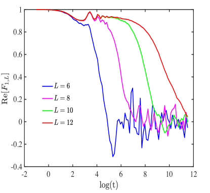
Figure S5: The OTOC ${\rm Re}[F_{1,L}(t)]$ between parafermions in the two open ends for increasing chain length $L=6,8,10,12$ with ED method . The parameter is $J_{2}=0.2,t_{\text{tol}}=10^{5}$ and the time is in the log scale.

References

- Nayak et al. (2008) Chetan Nayak, Steven H Simon, Ady Stern, Michael Freedman, and Sankar Das Sarma, “Non-abelian anyons and topological quantum computation,” Rev. Mod. Phys. 80, 1083 (2008).
- Kitaev (2003) A Yu Kitaev, “Fault-tolerant quantum computation by anyons,” Ann. Phys. 303, 2–30 (2003).
- Clarke et al. (2013) David J Clarke, Jason Alicea, and Kirill Shtengel, “Exotic non-abelian anyons from conventional fractional quantum hall states,” Nat. Commun. 4, 1348 (2013).
- Fendley (2012) Paul Fendley, “Parafermionic edge zero modes in Zn-invariant spin chains,” Journal of Statistical Mechanics: Theory and Experiment 2012, P11020 (2012).
- Alicea and Fendley (2016) Jason Alicea and Paul Fendley, “Topological phases with parafermions: theory and blueprints,” Annu. Rev. Condens. Matter Phys. 7, 119–139 (2016).
- Lindner et al. (2012) Netanel H Lindner, Erez Berg, Gil Refael, and Ady Stern, “Fractionalizing majorana fermions: Non-abelian statistics on the edges of abelian quantum hall states,” Phys. Rev. X 2, 041002 (2012).
- Vaezi (2013) Abolhassan Vaezi, “Fractional topological superconductor with fractionalized majorana fermions,” Phys. Rev. B 87, 035132 (2013).
- Vaezi (2014) Abolhassan Vaezi, “Superconducting analogue of the parafermion fractional quantum hall states,” Phys. Rev. X 4, 031009 (2014).
- Cheng (2012) Meng Cheng, “Superconducting proximity effect on the edge of fractional topological insulators,” Phys. Rev. B 86, 195126 (2012).
- Barkeshli and Qi (2014) Maissam Barkeshli and Xiao-Liang Qi, “Synthetic topological qubits in conventional bilayer quantum hall systems,” Phys. Rev. X 4, 041035 (2014).
- Stoudenmire et al. (2015) EM Stoudenmire, David J Clarke, Roger SK Mong, and Jason Alicea, “Assembling fibonacci anyons from a z3 parafermion lattice model,” Phys. Rev. B 91, 235112 (2015).
- Tsvelik (2014) AM Tsvelik, “Integrable model with parafermion zero energy modes,” Phys. Rev. Lett. 113, 066401 (2014).
- Klinovaja and Loss (2014) Jelena Klinovaja and Daniel Loss, “Parafermions in an interacting nanowire bundle,” Phys. Rev. Lett. 112, 246403 (2014).
- Zhang and Kane (2014) Fan Zhang and CL Kane, “Time-reversal-invariant z4 fractional josephson effect,” Phys. Rev. Lett. 113, 036401 (2014).
- Orth et al. (2015) Christoph P Orth, Rakesh P Tiwari, Tobias Meng, and Thomas L Schmidt, “Non-abelian parafermions in time-reversal-invariant interacting helical systems,” Phys. Rev. B 91, 081406 (2015).
- Alexandradinata et al. (2016) A Alexandradinata, N Regnault, Chen Fang, Matthew J Gilbert, and B Andrei Bernevig, “Parafermionic phases with symmetry breaking and topological order,” Phys. Rev. B 94, 125103 (2016).
- Alavirad et al. (2017) Yahya Alavirad, David Clarke, Amit Nag, and Jay D Sau, “Z3 parafermionic zero modes without andreev backscattering from the 2/3 fractional quantum hall state,” Phys. Rev. Lett. 119, 217701 (2017).
- Calzona et al. (2018) Alessio Calzona, Tobias Meng, Maura Sassetti, and Thomas L Schmidt, “Z4 parafermions in one-dimensional fermionic lattices,” Phys. Rev. B 98, 201110 (2018).
- Mazza et al. (2018) Leonardo Mazza, Fernando Iemini, Marcello Dalmonte, and Christophe Mora, “Nontopological parafermions in a one-dimensional fermionic model with even multiplet pairing,” Phys. Rev. B 98, 201109 (2018).
- Hutter and Loss (2016) Adrian Hutter and Daniel Loss, “Quantum computing with parafermions,” Phys. Rev. B 93, 125105 (2016).
- Alicea and Stern (2015) Jason Alicea and Ady Stern, “Designer non-abelian anyon platforms: from majorana to fibonacci,” Phys. Scr 2015, 014006 (2015).
- Chew et al. (2018) Aaron Chew, David F Mross, and Jason Alicea, “Fermionized parafermions and symmetry-enriched majorana modes,” Phys. Rev. B 98, 085143 (2018).
- Zhuang et al. (2015) Ye Zhuang, Hitesh J Changlani, Norm M Tubman, and Taylor L Hughes, “Phase diagram of the z3 parafermionic chain with chiral interactions,” Phys. Rev. B 92, 035154 (2015).
- Li et al. (2015) Wei Li, Shuo Yang, Hong-Hao Tu, and Meng Cheng, “Criticality in translation-invariant parafermion chains,” Phys. Rev. B 91, 115133 (2015).
- Kitaev (2001) A Yu Kitaev, “Unpaired majorana fermions in quantum wires,” Physics-Uspekhi 44, 131 (2001).
- Fu and Kane (2008) Liang Fu and Charles L Kane, “Superconducting proximity effect and majorana fermions at the surface of a topological insulator,” Phys. Rev. Lett. 100, 096407 (2008).
- Alicea et al. (2011) Jason Alicea, Yuval Oreg, Gil Refael, Felix Von Oppen, and Matthew PA Fisher, “Non-abelian statistics and topological quantum information processing in 1d wire networks,” Nat. Phys. 7, 412–417 (2011).
- Mong et al. (2014) Roger SK Mong, David J Clarke, Jason Alicea, Netanel H Lindner, Paul Fendley, Chetan Nayak, Yuval Oreg, Ady Stern, Erez Berg, Kirill Shtengel, et al., “Universal topological quantum computation from a superconductor-abelian quantum hall heterostructure,” Phys. Rev. X 4, 011036 (2014).
- (29) See Supplemental Material at [URL will be inserted by publisher] for details on the proof of , the MPO algorithm, analysis of the Hamiltonian symmetry and the dynamical symmetry, and for more numerical data.
- Hayden and Preskill (2007) Patrick Hayden and John Preskill, “Black holes as mirrors: quantum information in random subsystems,” J. High Energy Phys. 2007, 120 (2007).
- Sekino and Susskind (2008) Yasuhiro Sekino and Leonard Susskind, “Fast scramblers,” J. High Energy Phys. 2008, 065 (2008).
- Shenker and Stanford (2014) Stephen H Shenker and Douglas Stanford, “Black holes and the butterfly effect,” J. High Energy Phys. 2014, 67 (2014).
- Hosur et al. (2016) Pavan Hosur, Xiao-Liang Qi, Daniel A Roberts, and Beni Yoshida, “Chaos in quantum channels,” J. High Energy Phys. 2016, 4 (2016).
- Landsman et al. (2019) Kevin A Landsman, Caroline Figgatt, Thomas Schuster, Norbert M Linke, Beni Yoshida, Norm Y Yao, and Christopher Monroe, “Verified quantum information scrambling,” Nature 567, 61–65 (2019).
- Stöckmann (2000) Hans-Jürgen Stöckmann, “Quantum chaos: an introduction,” (2000).
- Altman (2018) Ehud Altman, “Many-body localization and quantum thermalization,” Nature Physics 14, 979–983 (2018).
- Nandkishore and Huse (2015) Rahul Nandkishore and David A Huse, “Many-body localization and thermalization in quantum statistical mechanics,” Annu. Rev. Condens. Matter Phys. 6, 15–38 (2015).
- Abanin et al. (2019) Dmitry A. Abanin, Ehud Altman, Immanuel Bloch, and Maksym Serbyn, “Colloquium: Many-body localization, thermalization, and entanglement,” Rev. Mod. Phys. 91, 021001 (2019).
- Lashkari et al. (2013) Nima Lashkari, Douglas Stanford, Matthew Hastings, Tobias Osborne, and Patrick Hayden, “Towards the fast scrambling conjecture,” Journal of High Energy Physics 2013, 22 (2013).
- Swingle and Chowdhury (2017) Brian Swingle and Debanjan Chowdhury, “Slow scrambling in disordered quantum systems,” Phys. Rev. B 95, 060201 (2017).
- Fan et al. (2017) Ruihua Fan, Pengfei Zhang, Huitao Shen, and Hui Zhai, “Out-of-time-order correlation for many-body localization,” Sci. Bull. 62, 707–711 (2017).
- Huang et al. (2017) Yichen Huang, Yong-Liang Zhang, and Xie Chen, “Out-of-time-ordered correlators in many-body localized systems,” Annalen der Physik 529, 1600318 (2017).
- Läuchli and Kollath (2008) Andreas M Läuchli and Corinna Kollath, “Spreading of correlations and entanglement after a quench in the one-dimensional bose–hubbard model,” Journal of Statistical Mechanics: Theory and Experiment 2008, P05018 (2008).
- Cheneau et al. (2012) Marc Cheneau, Peter Barmettler, Dario Poletti, Manuel Endres, Peter Schauß, Takeshi Fukuhara, Christian Gross, Immanuel Bloch, Corinna Kollath, and Stefan Kuhr, “Light-cone-like spreading of correlations in a quantum many-body system,” Nature 481, 484–487 (2012).
- Bohrdt et al. (2017) Annabelle Bohrdt, Christian B Mendl, Manuel Endres, and Michael Knap, “Scrambling and thermalization in a diffusive quantum many-body system,” New J. Phys. 19, 063001 (2017).
- Liu et al. (2018) Fangli Liu, James R Garrison, Dong-Ling Deng, Zhe-Xuan Gong, and Alexey V Gorshkov, “Asymmetric particle transport and light-cone dynamics induced by anyonic statistics,” Phys. Rev. Lett. 121, 250404 (2018).
- Stahl et al. (2018) Charles Stahl, Vedika Khemani, and David A Huse, “Asymmetric butterfly velocities in hamiltonian and circuit models,” arXiv:1812.05589 (2018).
- Zhang and Khemani (2020) Yong-Liang Zhang and Vedika Khemani, “Asymmetric butterfly velocities in 2-local hamiltonians,” SciPost Physics 9, 024 (2020).
- Zwolak and Vidal (2004) Michael Zwolak and Guifré Vidal, “Mixed-state dynamics in one-dimensional quantum lattice systems: a time-dependent superoperator renormalization algorithm,” Phys. Rev. Lett. 93, 207205 (2004).
- Verstraete et al. (2004) Frank Verstraete, Juan J Garcia-Ripoll, and Juan Ignacio Cirac, “Matrix product density operators: Simulation of finite-temperature and dissipative systems,” Phys. Rev. Lett. 93, 207204 (2004).
- Vidal (2007) Guifré Vidal, “Classical simulation of infinite-size quantum lattice systems in one spatial dimension,” Phys. Rev. Lett. 98, 070201 (2007).
- Schollwöck (2011) Ulrich Schollwöck, “The density-matrix renormalization group in the age of matrix product states,” Ann. Phys. 326, 96–192 (2011).
- Xu and Swingle (2020) Shenglong Xu and Brian Swingle, “Accessing scrambling using matrix product operators,” Nat. Phys. 16, 199–204 (2020).
- White et al. (2018) Christopher David White, Michael Zaletel, Roger SK Mong, and Gil Refael, “Quantum dynamics of thermalizing systems,” Phys. Rev. B 97, 035127 (2018).
- Hémery et al. (2019) Kévin Hémery, Frank Pollmann, and David J Luitz, “Matrix product states approaches to operator spreading in ergodic quantum systems,” Phys. Rev. B 100, 104303 (2019).
- Klinovaja et al. (2014) Jelena Klinovaja, Amir Yacoby, and Daniel Loss, “Kramers pairs of majorana fermions and parafermions in fractional topological insulators,” Phys. Rev. B 90, 155447 (2014).
- Jordan and Wigner (1993) Pascual Jordan and Eugene Paul Wigner, “über das paulische äquivalenzverbot,” in The Collected Works of Eugene Paul Wigner (Springer, 1993) pp. 109–129.
- Lieb and Robinson (1972) Elliott H Lieb and Derek W Robinson, “The finite group velocity of quantum spin systems,” in Statistical mechanics (Springer, 1972) pp. 425–431.
- Jermyn et al. (2014) Adam S Jermyn, Roger SK Mong, Jason Alicea, and Paul Fendley, “Stability of zero modes in parafermion chains,” Phys. Rev. B 90, 165106 (2014).
- Moran et al. (2017) Niall Moran, Domenico Pellegrino, JK Slingerland, and Graham Kells, “Parafermionic clock models and quantum resonance,” Phys. Rev. B 95, 235127 (2017).
- Swingle et al. (2016) Brian Swingle, Gregory Bentsen, Monika Schleier-Smith, and Patrick Hayden, “Measuring the scrambling of quantum information,” Phys. Rev. A 94, 040302 (2016).
- Zhu et al. (2016) Guanyu Zhu, Mohammad Hafezi, and Tarun Grover, “Measurement of many-body chaos using a quantum clock,” Phys. Rev. A 94, 062329 (2016).
- Yao et al. (2016) Norman Y Yao, Fabian Grusdt, Brian Swingle, Mikhail D Lukin, Dan M Stamper-Kurn, Joel E Moore, and Eugene A Demler, “Interferometric approach to probing fast scrambling,” arXiv preprint arXiv:1607.01801 (2016).
- Halpern (2017) Nicole Yunger Halpern, “Jarzynski-like equality for the out-of-time-ordered correlator,” Phys. Rev. A 95, 012120 (2017).
- Halpern et al. (2018) Nicole Yunger Halpern, Brian Swingle, and Justin Dressel, “Quasiprobability behind the out-of-time-ordered correlator,” Phys. Rev. A 97, 042105 (2018).
- Campisi and Goold (2017) Michele Campisi and John Goold, “Thermodynamics of quantum information scrambling,” Phys. Rev. E 95, 062127 (2017).
- Yoshida and Kitaev (2017) Beni Yoshida and Alexei Kitaev, “Efficient decoding for the hayden-preskill protocol,” arXiv preprint arXiv:1710.03363 (2017).
- Gärttner et al. (2017) Martin Gärttner, Justin G Bohnet, Arghavan Safavi-Naini, Michael L Wall, John J Bollinger, and Ana Maria Rey, “Measuring out-of-time-order correlations and multiple quantum spectra in a trapped-ion quantum magnet,” Nat. Phys. 13, 781–786 (2017).
- Wei et al. (2018) Ken Xuan Wei, Chandrasekhar Ramanathan, and Paola Cappellaro, “Exploring localization in nuclear spin chains,” Phys. Rev. Lett. 120, 070501 (2018).
- Li et al. (2017) Jun Li, Ruihua Fan, Hengyan Wang, Bingtian Ye, Bei Zeng, Hui Zhai, Xinhua Peng, and Jiangfeng Du, “Measuring out-of-time-order correlators on a nuclear magnetic resonance quantum simulator,” Phys. Rev. X 7, 031011 (2017).
- Peterson et al. (2015) Michael R Peterson, Yang-Le Wu, Meng Cheng, Maissam Barkeshli, Zhenghan Wang, and Sankar Das Sarma, “Abelian and non-abelian states in = 2/3 bilayer fractional quantum hall systems,” Phys. Rev. B 92, 035103 (2015).
- Maghrebi et al. (2015) Mohammad F Maghrebi, Sriram Ganeshan, David J Clarke, Alexey V Gorshkov, and Jay Deep Sau, “Parafermionic zero modes in ultracold bosonic systems,” Phys. Rev. Lett. 115, 065301 (2015).
- Vidal (2004) Guifré Vidal, “Efficient simulation of one-dimensional quantum many-body systems,” Phys. Rev. Lett. 93, 040502 (2004).
- Haake (1991) Fritz Haake, “Quantum signatures of chaos,” in Quantum Coherence in Mesoscopic Systems (Springer, 1991) pp. 583–595.