Hilbert Series, Machine Learning, and Applications to Physics

Abstract

We describe how simple machine learning methods successfully predict geometric properties from Hilbert series (HS). Regressors predict embedding weights in projective space to ${\sim}1$ mean absolute error, whilst classifiers predict dimension and Gorenstein index to $>90\%$ accuracy with ${\sim}0.5\%$ standard error. Binary random forest classifiers managed to distinguish whether the underlying HS describes a complete intersection with high accuracies exceeding $95\%$. Neural networks (NNs) exhibited success identifying HS from a Gorenstein ring to the same order of accuracy, whilst generation of “fake” HS proved trivial for NNs to distinguish from those associated to the three-dimensional Fano varieties considered.

I Introduction and Summary

The Hilbert series (HS) is an important invariant in the study of modern geometry. In physics, HS have recently become a powerful tool in high energy theory, appearing, for example, in the study of: Bogomol’nyi–Prasad–Sommerfield (BPS) operators of supersymmetric gauge theories Benvenuti:2006qr ; Feng:2007ur ; supersymmetric quantum chromodynamics (SQCDs) Gray:2008yu ; Hanany:2008sb ; Chen:2011wn ; Jokela:2011vg and instanton moduli spaces Benvenuti:2010pq ; Hanany:2012dm ; Buchbinder:2019eal ; invariants of the standard model Hanany:2010vu ; Lehman:2015coa ; polytopes which arise in string compactifications Braun:2012qc ; and explicit constructions of effective Lagrangians Lehman:2015via ; Henning:2015daa ; Kobach:2017xkw ; Anisha:2019nzx ; Marinissen:2020jmb ; Graf:2020yxt .

In parallel, a programme to use machine learning (ML) techniques to study mathematical structures has recently been proposed He:2017aed ; He:2018jtw ; DavEtAl21 . The initial studies were inspired by timely and independent works He:2017aed ; He:2017set ; Krefl:2017yox ; Ruehle:2017mzq ; Carifio:2017bov . In these, the effectiveness of ML regressor and classifier techniques in various branches of mathematics and mathematical physics has been investigated. Applications of ML include: finding bundle cohomology on varieties Ruehle:2017mzq ; Brodie:2019dfx ; Larfors:2020ugo ; distinguishing elliptic fibrations He:2019vsj and invariants of Calabi–Yau threefolds Bull:2018uow ; the Donaldson algorithm for numerical Calabi–Yau metrics Ashmore:2019wzb ; the algebraic structures of groups and rings He:2019nzx ; arithmetic geometry and number theory Alessandretti:2019jbs ; He:2020eva ; He:2020kzg ; quiver gauge theories and cluster algebras Bao:2020nbi ; patterns in particle masses Gal:2020dyc ; statistical predictions and model-building in string theory Deen:2020dlf ; Halverson:2019tkf ; Halverson:2020opj ; and classifying combinatorial properties of finite graphs He:2020fdg . Here we apply ML techniques to the plethystic programme of using Hilbert series to understand structures of quantum field theory. The physical motivation for this work has two primary applications. First, when considering a generic supersymmetric quantum field theory the number of BPS operators at each order is given by the initial terms in the Hilbert series. Computing these operator frequencies requires significant computational power, particularly for higher order terms (for the multi-trace case the growth is exponential). In this work the goal for the machine learning techniques implemented is to return information about the full series’ closed form, which can then directly provide the higher order information, hence bypassing the need for order-by-order computation. Second, from a string perspective the geometry of the moduli space has an array of physical applications and if these techniques can return the underlying variety’s geometric properties directly the vacuum can be analysed without need for complete information about the theory.

We examined databases of HS arising in geometry – see ABR:Fano ; BK22 and the Graded Ring Database (GRDB) grdb – and “fake” HS generated to imitate the “real” geometric HS. Simple ML methods were able to successfully predict several geometric quantities associated to the HS, and were able to accurately distinguish real from fake HS.

Depending on the form of the HS, simple regression neural networks (NNs) managed to learn the embedding weights in projective space to mean absolute error (MAE) ${\sim}1$; whilst classification NNs predicted the dimension and Gorenstein index with both accuracy and Matthews correlation coefficient (MCC) in excess of $0.9$.

Motivated by the question of whether ML can detect when a HS comes from a Gorenstein ring, we found that binary classifiers identified whether a fake HS had a palindromic numerator to accuracy and MCC greater than $0.9$. Binary classifiers were easily able to distinguish the fake generated data from the dataset of HS associated to three-dimensional Fano varieties obtained from grdb ; fanodata .

A random forest classifier correctly predicted whether the HS described a complete intersection (CI): this was achieved with accuracy $0.9$ and MCC $0.8$ when the numerator (padded with $0$’s) of the HS was used as input; and with accuracy $0.95$ and MCC greater than $0.9$ when the Taylor series (to order $100$) of the HS was used.

Code scripts for these investigations, along with the datasets generated and analysed, are available from:

https://github.com/edhirst/HilbertSeriesML.git

II Hilbert Series and Physics

The HS is an important quantity that encodes numerical properties of a projective algebraic variety. It is not a topological invariant in that it depends on the embedding under consideration (Harris, , Example 13.4). We work throughout with varieties defined over $\mathbb{C}$.

Given a complex projective variety $X$ and ample divisor $D$ there exists a natural embedding in a weighted projective space (w.p.s.) $\mathbb{P}_{\mathbb{C}}(p_{0},\ldots,p_{k})$. We denote its homogeneous coordinate ring by $R$, i.e. $R=\mathbb{C}[X_{0},\ldots,X_{k}]/I$ where the variables $X_{i}$ have weights $p_{i}$, and $I$ is the homogeneous ideal generated by the polynomials defining $X$. We write $\mathbb{P}_{\mathbb{C}}(p_{0}^{q_{0}},\ldots,p_{s}^{q_{s}})$ as shorthand to indicate that the weight $p_{i}$ appears $q_{i}$ times. The embedding of $X$ into the w.p.s. induces a grading on $R=\bigoplus_{i\geq 0}R_{i}$. We refer to Dolga for details.

The HS is the generating function for the dimensions of the graded pieces of $R$:

$$H(t;X)=\sum\limits_{i=0}^{\infty}(\dim_{\mathbb{C}}R_{i})t^{i}$$

where $\dim_{\mathbb{C}}R_{i}$, the dimension of the $i$-th graded piece of the ring $R$, can be thought of as the number of independent degree $i$ polynomials on the variety $X$. The map $i\mapsto\dim_{\mathbb{C}}R_{i}$ is called the Hilbert function.

By the Hilbert–Serre Theorem (see for example (AtiyahMacdonald, , Theorem 11.1)) there exists $P\in\mathbb{Z}[t]$ such that

$$H(t;X)=\frac{P(t)}{\prod\limits_{i=0}^{s}(1-t^{p_{i}})^{q_{i}}}.$$ (1)

Let $j$ be the smallest positive multiple such that $jD$ is very ample. We call $j$ the Gorenstein index, and can rewrite (1) in the form:

$$H(t;X)=\frac{\tilde{P}(t)}{(1-t^{j})^{\dim+1}}$$ (2)

Here $\dim$ is the dimension of $X$, and $\tilde{P}\in\mathbb{Z}[t]$. If $R$ is a Gorenstein graded ring then the numerator is a palindromic polynomial (by Serre duality). Recall that a polynomial $\sum_{i=1}^{d}a_{i}t^{i}$ is called palindromic if $a_{i}=a_{d-i}$ Stanley1978 .

For example, consider the complex line $M=\mathbb{C}$ (regarded as the affine cone over a point) parameterised by a single complex variable $x$. Then the $i$-th graded piece $R_{i}$ is generated by the single monomial $x^{i}$. Thus, $\dim_{\mathbb{C}}R_{i}=1$ for all $i\in\mathbb{Z}_{\geq 0}$ so that the HS becomes $H(t;\mathbb{C})=(1-t)^{-1}$. In general, we have that $H(t;\mathbb{C}^{n})=(1-t)^{-n}$.

The Plethystic Programme. In supersymmetric gauge theories, when the vevs of scalars in different supermultiplets are turned on, the (vacuum) moduli spaces are non-trivial algebraic varieties vms ; LT ; Mehta:2012wk such as hyperkähler cones and (closures of) symplectic leaves. In this case HS are a powerful tool to enumerate gauge invariant operators (GIOs) at different orders.

A particularly useful application of HS to theoretical physics is the plethystic programme, which reveals more information of the moduli spaces. We leave a detailed summary of the key formulae to Appendix A.

The multi-graded HS, i.e. the multi-variate series

$$H(t_{1},\dots,t_{k};X)=\sum\limits_{\vec{i}=0}^{\infty}\dim_{\mathbb{C}}(X_{\vec{i}})t_{1}^{i_{1}}\dots t_{k}^{i_{k}}$$

obtained by considering multi-graded rings with pieces $X_{\vec{i}}$ for $\vec{i}=(i_{1},\dots,i_{k})$, could fully determine how the GIOs transform under symmetry groups of gauge theories.

Duality and Moduli Spaces. HS have been well-studied in the context of quiver gauge theories. For Higgs branches in low dimensions, HS obtained from the Molien–Weyl integral enable us to systematically study the geometry of SQCDs Gray:2008yu . Such methods can also be used to study the instanton moduli spaces Benvenuti:2010pq ; Hanany:2012dm ; Dey:2013fea . As the spaces of dressed monopole operators, i.e. the Coulomb branches, receive quantum corrections, monopole formula Cremonesi:2013lqa and Hall–Littlewood formula Cremonesi:2014kwa are used to obtain the HS. This not only unveils the geometry of moduli spaces, but also provides tools and evidences to study three-dimensional mirror symmetry and duality including theories in higher dimensions.

Standard Model. Phenomenologically, HS have been applied to lepton and quark flavour invariants for the Standard Model in Hanany:2010vu as well as to the minimal supersymmetric Standard Model in He:2014loa ; Xiao:2019uhh .

III Machine Learning

In this section we describe our approaches to ML properties of the rational representations (1) and (2) by feeding in coefficients of the corresponding HS. Keras with the TensorFlow backend Tensorflow was used for the investigations. In §III.1, “real” HS associated to certain three-dimensional Fano varieties are introduced and analysed. In §III.2, “fake” HS, i.e. rational functions of the form (1) and (2), were generated and properties of them were machine-learnt. In §III.3 and §III.4, binary classifiers were used to determine whether fake HS of the form (2) had palindromic numerator, and to determine fake HS from real HS, all with great success. Finally, in §III.5 we use ML to determine if a HS is associated to a complete intersection.

III.1 Acquiring HS

Example HS associated to algebraic varieties were retrieved from the GRDB grdb ; fanodata . We use a database of candidate HS conjecturally associated to three-dimensional $\mathbb{Q}$-Fano varieties with Fano index one, as constructed in ABR:Fano ; BK22 . Such varieties come with a natural choice of ample divisor $D=-K$, the anti-canonical divisor. We call these HS “real”. See Appendix B for the distributions of the parameters $d,\{a_{i}\},s,\{p_{\ell}\},\{q_{\ell}\}$ for this set of data. Here we are using notation as in (1), and write $P(t)=1+\sum_{i=1}^{d}a_{i}t^{i}$ for the numerator polynomial.

Example 1

Consider the three-dimensional $\mathbb{Q}$-Fano variety $X\subset\mathbb{P}(1^{3},2^{2},3^{2})$ (number $11122$ in the GRDB). This is of codimension $3$, with $\mathcal{B}=\{\frac{1}{2}(1,1,1),2\times\frac{1}{3}(1,1,2)\}$ isolated orbifold points, and hence has Gorenstein index $j=6$. Writing the HS in the form (1) gives:

$$H(t;X)=\frac{P(t)}{(1-t)^{3}(1-t^{2})^{2}(1-t^{3})^{2}}$$

$$\text{ where }P(t)=1-2t^{4}-2t^{5}+ 2t^{7}+2t^{8}-t^{12}.$$

Rewriting this in the form (2) gives:

$$H(t;X)=\frac{\tilde{P}(t)}{(1-t^{6})^{4}}$$

$$\text{ where }\tilde{P}(t)=1+ 3t+8t^{2}+\ldots+8t^{21}+3t^{22}+t^{23}.$$

For the HS of this dataset, there are two competing phenomena that contribute to its coefficients: the initial part $P_{\mathrm{ini}}$ that coincides with the HS in small degrees and the “correction terms” $P_{\mathrm{orb}}(Q)$ for each isolated orbifold point $Q=\frac{1}{r}(b_{1},\ldots,b_{\dim})$ of $X$. More precisely, we have icecream

$$H(t;X)=P_{\mathrm{ini}}+\sum_{Q\in\mathcal{B}}P_{\mathrm{orb}}(Q)$$

where the sum is taken over the set $\mathcal{B}$ of isolated orbifold points of $X$. $P_{\mathrm{ini}}$ and $P_{\mathrm{orb}}(Q)$ ($Q=\frac{1}{r}(b_{1},\ldots,b_{\dim})$) satisfy

$$P_{\mathrm{ini}}=\frac{A(t)}{(1-t)^{\dim+1}},\quad P_{\mathrm{orb}}(Q)=\frac{B_{Q}(t)}{(1-t)^{\dim}(1-t^{r})}$$

where $A(t),B_{Q}(t)$ are integral palindromic polynomials with degrees related via $\deg{B_{Q}(t)}-\deg{A(t)}=r-1$. The coefficients (called plurigenera) of the HS of $H$ coincide with $P_{\mathrm{ini}}$ in degrees $\leq\lfloor\deg{A(t)}/2\rfloor$, whilst in higher degrees the orbifold points start to contribute to the plurigenera. Because of this phenomenon, extra care must be taken when computing parameters for the representations (1) and (2) from a finite set of coefficients of the HS. Our investigations show that ML can cope with this behaviour.

III.2 Generating and ML Fake HS

The “fake” HS generated take the forms (1) and (2), with numerators of the form $1+\sum_{i=1}^{d}a_{i}t^{i}$. The numerator $\tilde{P}(t)$ of (2) is required to be palindromic (and, as a consequence, $a_{d}=1$). Coefficient sets consisting of the parameters $d,\{a_{i}\},s,\{p_{\ell}\},\{q_{\ell}\}$, where $1\leq i\leq d$ and $1\leq\ell\leq s$, were randomly generated and the Taylor expansions of the resulting fake HS were computed to order ${\sim}1000$. If the parameters did not satisfy $\sum_{\ell}p_{\ell}q_{\ell}>d$, if there were negative coefficients in the resulting Taylor expansion, or if they matched a real Hilbert series then the parameters were discarded.

The resulting data were fed into a NN to learn the desired properties of the fake HS. The input was a vector of Taylor expansion coefficients: either a vector of coefficients for low-order terms $0$ to $100$; or for high-orders terms $1000$ to $1009$. Although coefficients of low-order terms are easier to calculate, predictions based on those inputs are more error-prone as contributions from orbifold points take effect only for high-order terms (see §III.1).

Fewer coefficients were required when learning from coefficients deeper in the Taylor expansion; geometric data are more readily extracted from larger plurigenera. We found the following analogy from toric geometry insightful. When counting the number of lattice points $c_{m}=\left|m\Delta\cap\mathbb{Z}^{\dim}\right|$ in the $m$-th dilation of a polytope $\Delta$ then, for $m\gg 0$, $c_{m}\sim\mathrm{Vol}(m\Delta)=m^{\dim}\mathrm{Vol}(\Delta)$. (This is a toric rephrasing of the HS, with $\Delta$ the polytope associated with an ample divisor $D$ and $c_{m}=h^{0}(mD)$.)

The first investigation used supervised regressor NNs to learn $\{p_{\ell}\}$ for fake HS in the form (1). Supervised classifier NNs were trained to predict the Gorenstein index $j$ and the dimension $\dim$ of fake HS in the form (2). Classifiers were used since the NN outputs were single numbers and hence associated well to classifier data structures.

We conclude with a comparison of the collected fake HS data with the real HS data from the GRDB. We use the unsupervised method of principal component analysis (PCA) to project the classes onto the highest variance linear component (see Figure 1). The PCA was performed on the vectors of the first 100 coefficients, with prior scalar transformation. The explained variance ratios give the normalised eigenvalues for the covariance matrix, sorted into a decreasing order. For the fake to real HS comparison the first eigenvalue ($0.78$) was significantly larger than the second ($0.16$) and subsequent 98 eigenvalues ($<0.04$). This indicates that one principal component is sufficient for description of the data distribution, and this principal component pays linearly progressively more attention to coefficients throughout the input HS vector up to the 24th where it then considers equal contributions from the remaining coefficients.

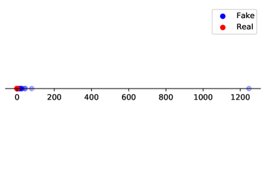
Figure 1: PCA for HS Taylor expansion coefficients coming from the GRDB, ‘Real’, or those randomly generated, ‘Fake’.

The projection shows a separation between the classes, indicating that there is linear structure in the data. Despite great efforts we were unable to break this separation. This raises the following question, to which we do not currently know the answer: what additional properties do fake HS need to satisfy to better approximate the GRDB HS data?

HS Regressor Investigations. For this investigation ${\sim}10\,000$ fake HS of the form (1) were uniformly drawn from a sample space given by $d=3$, $s=3$, $|a_{i}|\leq 10$, $p_{\ell}\leq 10$. This space was chosen to provide a sufficiently large range of fake HS whilst ensuring that its size was still feasible for ML training. The goal was to predict the values $\{p_{\ell}\}$ and $\{q_{\ell}\}$ of the form (1) from a given (finite) range of HS coefficients. This information was encoded into a single vector where each $p_{\ell}$ was repeated $q_{\ell}$ times, and the entries were given in increasing order.

A $5$-fold cross-validation (in the sense of friedman2001elements ) was performed for a feed-forward regressor NN with $4$ hidden dense layers of $1024$ neurons each, using LeakyReLU activation (with $\alpha=0.01$), in batches of $32$ for $20$ epochs over the full dataset. The NN had a final dense layer with as many neurons as $p_{\ell}$’s (counting multiplicities). Dropout layers between the dense layers reduced the risk of overfitting (dropout factor $0.05$). The NN was trained with the Adam optimiser Adam using a log(cosh) loss function and the training performance was measured via MAE. log(cosh) is a continuous version of MAE used as the loss function such that training performance would be improved for gradient descent near the MAE discontinuity, however MAE provides a more interpretable metric of learning performance so is used as the metric on the independent test data.

Table 1 summarises the averaged MAE, with standard error, over the $5$-fold cross validation for two ranges of HS coefficients: the first $101$ coefficients; and the coefficients of order $1000$ to $1009$. In both cases the MAE is below $2$, i.e. the true denominator of the form (1) of the underlying HS could be extracted with reasonably good accuracy from the HS coefficients alone.

Orders of Input	MAE
$0$ to $100$	$1.94\pm 0.11$
$1000$ to $1009$	$1.04\pm 0.12$

Table 1: Averaged MAE, with standard error, of the $5$-fold cross-validation of the NN learning the weights $p_{\ell}$ (with multiplicity) of the form (1) of the HS from input vectors of HS coefficients to the specified orders.

HS Classification Investigations. In this investigation a $5$-fold cross-validation for a feed-forward classifier NN with the same layer structure as before was trained. We again used an Adam optimiser, but now with sparse categorical cross entropy loss to reflect the classification question. Training performance was measured with accuracy and MCC. The final dense layer now had as many neurons as classes in the investigation (5 in both cases), with softmax activation, and neurons representing the values the learnt parameters could take.

This time ${\sim}10\,000$ HS of the form (2) were uniformly drawn from a sample space given by $d=5$, $|a_{i}|\leq 50$, $j\leq 5$, $\dim\leq 5$. The goal this time was to train an NN to predict the Gorenstein index $j$, the dimension $\dim$, and the form (2) from the HS coefficients in the same orders of degrees.

Note if coefficients in larger degrees were used as input, the larger values caused problems with the loss function. This issue was mitigated by log-normalising the HS coefficients, i.e. by taking the natural logarithm input values were scaled down to ranges the loss function and optimiser could handle. However some fake HS contained $0$ coefficients and were therefore omitted, hence resulting in a full dataset of $8711$ HS for the training with HS coefficients of larger degree. Note also that log-normalisation was only used in this case and in no other investigations.

Table 2 summarises the averaged accuracies and MCCs, with standard error, over the $5$-fold cross-validation of the NN. These results show almost perfect classification of both the Gorenstein index, $j$, and the dimension, dim, from HS coefficients in low degrees. Interestingly the performance is worse when using terms deeper in the HS, presumably due to the required log-normalisation of the coefficients removing the finer structure of the coefficients required to determine the exact parameter value being learnt.

Parameter	Orders	Performance Measures
Learnt	of Input	Accuracy	MCC
$j$	$0$ to $100$	$0.934\pm 0.008$	$0.916\pm 0.010$
	$1000$ to $1009$	$0.780\pm 0.018$	$0.727\pm 0.022$
dim	$0$ to $100$	$0.995\pm 0.005$	$0.993\pm 0.006$
	$1000$ to $1009$	$0.865\pm 0.024$	$0.822\pm 0.031$

Table 2: Averaged accuracy and MCC, with standard error, of the $5$-fold cross-validation of the NN learning the Gorenstein index $j$, the dimension $\dim$, and the form (2) with HS coefficients in the specified ranges of degrees as input.

III.3 Identifying the Gorenstein Property

In this section we investigate the effectiveness of binary classifiers to detect if the numerator of form (2) of an HS is palindromic. Recall from Section II that the numerator is palindromic if the ring $R$ is Gorenstein (by Serre duality). Then the numerator of form (1) is palindromic too (possibly up to a sign); see Example 1 for an illustration. The goal was to use a NN to distinguish whether a HS is coming from a Gorenstein ring, i.e. the numerator polynomial of form (2) is palindromic. As before the NN’s input were HS coefficients from the same ranges of degrees.

For the investigation two equally sized sets of fake HS, one with and the other without palindromic numerators, were uniformly drawn from a sample space given by $d=9$, $|a_{i}|\leq 50$, $j=5$, $\dim+1=6$. The same reasons as before apply for this choice of space. The HS in each of the two sets were then labelled and together comprised the full dataset for a $5$-fold cross-validation to be performed using a feed-forward classifier NN with the same layer structure as in the previous investigation. Also the same Adam optimiser was used for training, but now with binary cross-entropy loss to reflect the classification question. Training performance was measured with accuracy and MCC. The final dense layer of the NN now had $2$ neurons corresponding to whether the HS comes from a Gorenstein ring or not.

Table 3 summarises the averaged accuracies and MCCs, with standard error, over the $5$-fold cross-validation of the NN. The results show good success in detecting if a HS comes from a Gorenstein ring using HS coefficients alone. The classifier performed better on coefficients in larger degrees indicating that the palindromicity property is more readily evident from plurigenera deeper in the HS (possibly because of the bigger variation).

In addition, PCA was also applied to the data in this binary classification problem, as seen in Figure 2, with similar behaviour for both low and high orders of input. This figure (for the low order inputs) highlights a lack of linear structure which the architecture could take advantage of. The PCA explained variance ratios for the 101 low order inputs show equal importance of the first two principal components (0.29, 0.27), lower importance for the next three components (0.19, 0.11, 0.10), minimal importance of the next four components ($\sim 0.01$), then negligible contribution from the remaining 92 ($\lesssim 10^{-30}$). Equivalently for the high order inputs the first two components are dominant (0.30,0.26), with the next three less important (0.20,0.12,0.10), and the remaining five negligible ($\lesssim 10^{-10}$). In both cases the two dominant principal components have a mix of contributions from components with no discernible pattern across the HS vector of coefficients. The full outputs can be observed in this paper’s respective GitHub scripts.

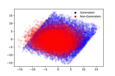
Figure 2: The PCA for HS Taylor expansion coefficients corresponding to HS defined over Gorenstein rings or non-Gorenstein rings.

Orders	Performance Measures
of Input	Accuracy	MCC
$0$ to $100$	$0.844\pm 0.087$	$0.717\pm 0.155$
$1000$ to $1009$	$0.954\pm 0.043$	$0.919\pm 0.073$

Table 3: Averaged accuracy and MCC, with standard error, of the $5$-fold cross-validation of a NN learning whether the HS has palindromic numerator in form (2) from HS coefficients to the specified orders as input.

III.4 Differentiating Real and Fake HS

This investigation examined the success of a binary classifier in distinguishing whether a HS, represented by a finite set of HS coefficients, corresponds to a real HS from the GRDB, or a randomly generated fake HS. The dataset consisted of HS candidates conjecturally associated to $3$-dimensional Fano polytopes from the GRDB, amounting to ${\sim}29\,000$ HS, along with as many fake HS with the same structure which were randomly generated.

A $5$-fold cross-validation for a feed-forward classifier NN with the same layer structure as in the previous investigations was performed. For training an Adam optimiser with a binary cross-entropy loss with the same parameters as before was used. Training performance was measured with accuracy and MCC. The final dense layer had $2$ neurons corresponding to whether the inputted HS coefficients were associated to a real or fake HS.

The ${\sim}29\,000$ fake HS were generated randomly using form (1) parameters drawn from probability distributions reflecting the real HS data as given in Appendix B. An equal number of real HS were taken from the GRDB to produce the full dataset, and as before HS coefficients to the same order of degrees were used as NN inputs.

In this investigation the averaged accuracies and MCCs exceeded $0.99$ for both ranges of degrees of HS coefficients. Further analysis of the data showed that coefficients of fake HS were orders of magnitudes different to the real case which possibly made this classification far easier. Resampling such that the coefficients were more comparable, although improving this investigations complexity, would make the fake data less representative with respect to the underlying variety’s properties. Hence we chose to use the same data throughout all investigations despite this binary classification becoming more trivial; as corroborated by the 1d PCA separation in Figure 1. This also highlights the uniqueness of real HS which come with a wealth of further impactful structure, e.g. on the parameters of the corresponding forms (1) and (2).

III.5 Detecting Complete Intersection

An important application of the plethystic logarithm (see Appendix A for details and references) is that it detects whether the underlying variety is a complete intersection (CI), i.e. the defining ideal (the ideal of polynomials vanishing on the variety) is generated by exactly codimension many polynomials. Such optimal intersection has been widely used in the physics literature, e.g. in string model-building Candelas:1987kf ; Anderson:2007nc . As can be seen from the definition, the $\text{PE}^{-1}$ involves the number-theoretic $\mu$-function, making the computation non-trivial. A natural question arises as to whether a trained classifier can identify whether $X$ is CI, i.e. when $\text{PE}^{-1}$ terminates as a Taylor series, by only “looking” at the the shape of the HS.

Suppose $X=\{f_{1}=0,\ldots,f_{c}=0\}$ defines a complete intersection in $\mathbb{P}_{\mathbb{C}}^{k}$ where each $f_{i}$ is a homogeneous polynomial of degree $m_{i}$ in a standard graded polynomial ring $R_{k+1}=\mathbb{C}[X_{0},\ldots,X_{k}]$, such that each variable $X_{i}$ has degree $1$. Then the HS of $X$ takes the form

$$\frac{\left(1-t^{m_{1}}\right)\dots\left(1-t^{m_{c}}\right)}{(1-t)^{n}}=\frac{1+a_{1}t+\dots+a_{d}t^{d}}{(1-t)^{n}}.$$ (3)

This follows by induction on the $f_{i}$ using the additivity of HS and the the exact sequences

$$0\to R_{k}^{[m_{i}]}\xrightarrow{\cdot f_{i}}R_{k}\to R_{k+1}\to 0$$

where $R_{k}^{[m_{i}]}$ denotes a standard graded polynomial ring with degrees shifted by $m_{i}$ so that the first map becomes a morphism of graded rings. Notice $X$ is a projective variety of codimension $c$ in $\mathbb{P}_{\mathbb{C}}^{k}$, i.e. has dimension $\dim=k-c$.

This time $10\,000$ fake HS of the form (3) representing CIs were uniformly drawn from a sample space given by $c=1,\ldots,10$, $m_{i}=2,\ldots,10$ and $1\leq n-\sum_{i}m_{i}\leq 11$. The fake HS representing non-CI were generated by drawing fake CI HS $f$ from the sample space above and then adding or subtracting a binomial to the numerator preventing the result to factor as in (3). More precisely, the fake non-CI HS were computed by

$$f+(-1)^{\varepsilon}\cdot\frac{t^{k_{0}}+(-1)^{c}\cdot t^{d-k_{0}}}{(1-t)^{n}}$$

where $\varepsilon=0,1$ and $k_{0}=1,\dots,d-1$ was randomly chosen. This procedure ensured that learning is non-trivial, because the resulting fake non-CI HS have a similar shape to the form (3), but do not correspond to fake HS of CI. The full dataset was comprised by $10\,000$ fake CI HS and $10\,000$ fake non-CI HS, i.e. a total of $20\,000$ samples.

We use quotients of successive coefficients in the Taylor expansion of the fake HS as input to see if the machine could identify complete intersections, i.e. we use

$$\{h_{i}/h_{i+1}\mid i=0,\dots,n\}$$

where $h_{i}$ denotes the $i$-th coefficient in the Taylor expansion of the fake HS and $n$ is the number of coefficients used. We use PCA to reduce the dimension followed by a random forest classifier or a NN. Table 4 summarises the averaged accuracies and MCCs, with standard error, over $10$-fold cross-validations (training performed on the $10\%$ chunks).

ML	Orders	Performance Measures
algorithm	of Input	Accuracy	MCC
PCA+NN	$0$ to $100$	$0.762\pm 0.010$	$0.544\pm 0.030$
	$0$ to $300$	$0.951\pm 0.005$	$0.902\pm 0.010$
PCA+RF	$0$ to $100$	$0.806\pm 0.016$	$0.615\pm 0.031$
	$0$ to $300$	$0.965\pm 0.003$	$0.930\pm 0.005$

Table 4: Averaged accuracy and MCC, with standard error, of the $10$-fold cross-validation of the PCA+random forest (resp. of the PCA+NN) learning complete intersections in the form (3) with fake HS coefficients in the specified ranges of degrees as input.

If we truncate the Taylor series at order $100$ and train on $10\%$ of the data, the accuracy is ${\sim}0.80$ with MCC ${\sim}0.61$. However, including higher and higher orders of coefficients results into more and more improved results (where the increase in improvement stagnates for sufficiently high orders). For example, if we use Taylor expansions to order $300$ and train on $10\%$ of the data, the PCA+random forest model could give over $0.95$ accuracy and over $0.9$ MCC. More precisely, a $10$-fold cross validation (with training performed on the $10\%$ chunks) would give $0.965(\pm 0.002)$ accuracy (with $95\%$ confidence interval). We can reproduce these results by using PCA and a feed-forward NN with $4$ hidden dense layers of $32$ neurons each, dropout layers between the dense layers (dropout factor $0.05$), LeakyReLU activation (with $\alpha=0.01$), binary cross-entropy loss function and Adam optimiser. A $10$-fold cross validation with the same input (training performed on the $10\%$ chunks) yields $0.951(\pm 0.004)$ accuracy (with $95\%$ confidence interval).

PCA shows a clear separation of CIs and non-CIs (see Figure 3). The explained variance ratios show one dominant component with eigenvalue 0.98, where this component has roughly equal contributions from all the series coefficients. This raises the question if this implies that PCA can efficiently separate CI from non-CI (real) HS or if this is an artefact of our data generation. With 20000 samples of CIs and real non-CIs, we find that a random forest could give $\sim 0.8$ accuracy and $\sim 0.6$ MCC for a 10-fold cross validation. Although this is a decent result, it would be natural to investigate in future whether there could be better techniques/algorithms to improve such performance. Further study is also necessary to confirm that PCA is an effective discriminator between CI and non-CI in this case.

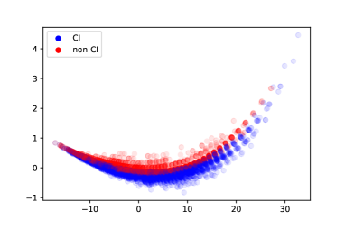
Figure 3: PCA for complete and non-complete intersections (with successive quotients of Taylor coefficients).

Acknowledgements. JB is supported by a CSC scholarship. YHH would like to thank STFC for grant ST/J00037X/1. EH would like to thank STFC for a PhD studentship. JH is supported by a Nottingham Research Fellowship. AK is supported by EPSRC Fellowship EP/N022513/1. SM is funded by a SMCSE Doctoral Studentship. This collaboration was made possible by a Focused Research Workshop grant from the Heilbronn Institute for Mathematical Research.

Appendix A The Plethystic Programme

For a function $f(t)=\sum\limits_{n=0}^{\infty}a_{n}t^{n}$, we can define the plethystic exponential (sometimes known as the Euler transform) as

$$\text{PE}[f(t)]\coloneqq\exp\left(\sum_{n=1}^{\infty}\frac{f(t^{n})-f(0)}{n}\right)={\prod\limits_{n=1}^{\infty}(1-t^{n})^{-a_{n}}}.$$

For instance, the mesonic BPS operators fall into two categories: single- and multi-trace. Then the HS is the generating function for counting the basic single-trace invariants. Moreover, the HS of the $N$-th symmetric product is given by $g_{N}(t;M)=f(t;{\rm sym}^{N}(X)),~{}{\rm sym}^{N}(X):=M^{N}/S_{N}\ ,$ where the “grand-canonical” partition function is given by the fugacity-inserted plethystic exponential of the Hilbert series: $\text{PE}\nu[f(t)]:=\prod\limits_{n=0}^{\infty}{(1-\nu\,t^{n})^{-a_{n}}}=\sum\limits_{N=0}^{\infty}g_{N}(t)\nu^{N}$. In gauge theory, this is considered to be at finite $N$ and the expansion $g_{N}(t)=\sum\limits_{n=0}^{\infty}b_{n}t^{n}$ gives the number $b_{n}$ of operators of charge $n$.

There is also an analytic inverse function to PE, which is the plethystic logarithm, given by

$$\text{PE}^{-1}[g(t)]=\sum_{k=1}^{\infty}\frac{\mu(k)}{k}\log(g(t^{k})),$$

where $\mu(k)$ is the Möbius function. The first positive terms in the Taylor expansion of PE^-1 encodes generators at different degrees, and the first negative terms give the relations among them. Higher order terms are known as the syzygies. In particular, if $X$ is a complete intersection, then $\text{PE}^{-1}[H(t)]$ is a polynomial of $t$ (i.e. terminates at a finite order).

Appendix B Real HS parameter distributions

The dataset of real HS associated to $3$-dimensional Fano varieties considered in this paper grdb that was analysed to produce distributions of the HS function form parameters $d,\{a_{i}\},s,\{p_{\ell}\},\{q_{\ell}\}$ as shown in Figures 4-8. These distributions, and their respective fittings were used to make fake HS generation more representative of the real HS data.

Fittings used sums of Gaussian distributions, reflecting a Central Limit Theorem motivation in analysis of this large dataset of ${\sim}54\,000$ HS. In all cases the sum of $2$ independent Gaussian distributions sufficed in making a visually accurate fit. Thus, using these distribution in fake HS generation would ideally produce HS of the same form. Interestingly, the fake HS still had quite different coefficient growth rates to the real HS, stabilising deeper in the series. This phenomena is further discussed in §III.4.

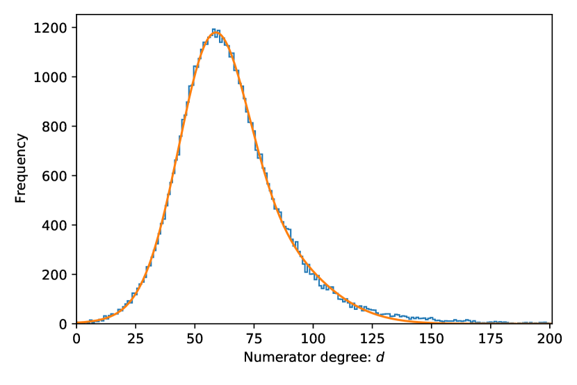
Figure 4: Histogram of distribution of real HS numerator degrees $d$, with Gaussian fitting.

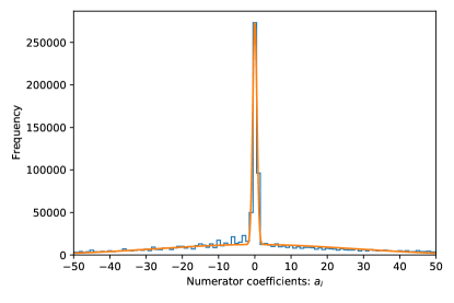
Figure 5: Histogram of distribution of real HS numerator coefficient values $a_{i}$, with Gaussian fitting.

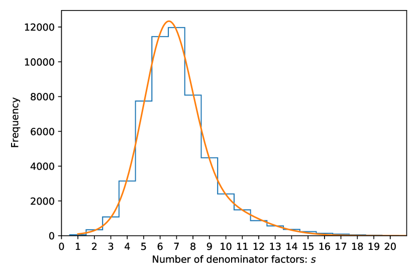
Figure 6: Histogram of distribution of real HS number of denominator factors $s$, with Gaussian fitting.

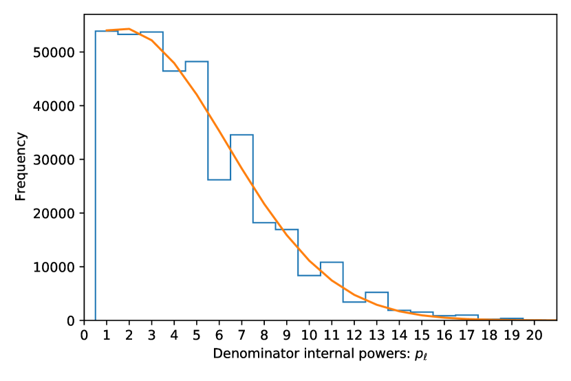
Figure 7: Histogram of distribution of real HS denominator internal powers (i.e. denominator weights) $p_{\ell}$, with Gaussian fitting.

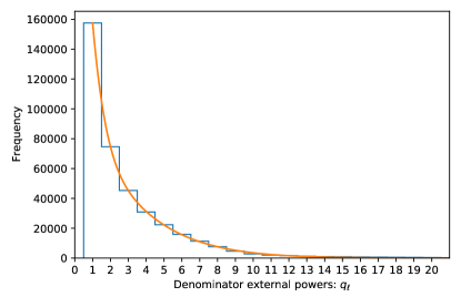
Figure 8: Histogram of distribution of real HS denominator external powers (i.e. number of repetitions of each denominator weight) $q_{\ell}$, with Gaussian fitting.

References

- (1) S. Benvenuti, B. Feng, A. Hanany, and Y.-H. He, “Counting BPS operators in gauge theories: quivers, syzygies and plethystics,” J. High Energy Phys. no. 11, (2007) 050, 48.
- (2) B. Feng, A. Hanany, and Y.-H. He, “Counting gauge invariants: the plethystic program,” J. High Energy Phys. no. 3, (2007) 090, 42.
- (3) J. Gray, Y.-H. He, A. Hanany, N. Mekareeya, and V. Jejjala, “SQCD: a geometric aperçu,” Journal of High Energy Physics 2008 no. 05, (May, 2008) 099–099.
- (4) A. Hanany, N. Mekareeya, and G. Torri, “The Hilbert series of adjoint SQCD,” Nuclear Phys. B 825 no. 1-2, (2010) 52–97.
- (5) Y. Chen and N. Mekareeya, “The Hilbert series of U/SU SQCD and Toeplitz determinants,” Nuclear Phys. B 850 no. 3, (2011) 553–593.
- (6) N. Jokela, M. Järvinen, and E. Keski-Vakkuri, “New results for the SQCD Hilbert series,” J. High Energy Phys. no. 3, (2012) 048, front matter+30.
- (7) S. Benvenuti, A. Hanany, and N. Mekareeya, “The Hilbert series of the one instanton moduli space,” J. High Energy Phys. no. 6, (2010) 100, 40.
- (8) A. Hanany, N. Mekareeya, and S. S. Razamat, “Hilbert series for moduli spaces of two instantons,” J. High Energy Phys. no. 1, (2013) 070, front matter + 48.
- (9) E. I. Buchbinder, A. Lukas, B. A. Ovrut, and F. Ruehle, “Instantons and Hilbert Functions,” Phys. Rev. D 102 no. 2, (2020) 026019, arXiv:1912.08358 [hep-th].
- (10) A. Hanany, E. E. Jenkins, A. V. Manohar, and G. Torri, “Hilbert series for flavor invariants of the Standard Model,” J. High Energy Phys. no. 3, (2011) 096, 7.
- (11) L. Lehman and A. Martin, “Low-derivative operators of the Standard Model effective field theory via Hilbert series methods,” Journal of High Energy Physics 02 no. 81, (2016) .
- (12) V. Braun, “Counting points and Hilbert series in string theory,” in Strings, gauge fields, and the geometry behind, pp. 225–235. World Sci. Publ., Hackensack, NJ, 2013.
- (13) L. Lehman and A. Martin, “Hilbert series for constructing lagrangians: Expanding the phenomenologist’s toolbox,” Phys. Rev. D 91 (May, 2015) 105014.
- (14) B. Henning, X. Lu, T. Melia, and H. Murayama, “Hilbert series and operator bases with derivatives in effective field theories,” Comm. Math. Phys. 347 no. 2, (2016) 363–388.
- (15) A. Kobach and S. Pal, “Hilbert series and operator basis for NRQED and NRQCD/HQET,” Phys. Lett. B 772 (2017) 225–231.
- (16) Anisha, S. Das Bakshi, J. Chakrabortty, and S. Prakash, “Hilbert series and plethystics: paving the path towards 2HDM- and MLRSM-EFT,” J. High Energy Phys. no. 9, (2019) 035, 113.
- (17) C. B. Marinissen, R. Rahn, and W. J. Waalewijn, “, 83106786, 114382724, 1509048322, 2343463290, 27410087742, efficient Hilbert series for effective theories,” Phys. Lett. B 808 (2020) 135632, 7.
- (18) L. Graf, B. Henning, X. Lu, T. Melia, and H. Murayama, “2, 12, 117, 1959, 45171, 1170086, …: a Hilbert series for the QCD chiral Lagrangian,” JHEP 01 (2021) 142, arXiv:2009.01239 [hep-ph].
- (19) Y.-H. He, “Deep-learning the landscape.” arXiv:1706.02714 [hep-th], 2017.
- (20) Y.-H. He, “The Calabi–Yau landscape: from geometry, to physics, to machine-learning.” arXiv:1812.02893 [hep-th], 2018.
- (21) A. Davies, P. Veličković, L. Buesing, S. Blackwell, D. Zheng, N. Tomašev, R. Tanburn, P. Battaglia, C. Blundell, A. Juhász, M. Lackenby, G. Williamson, D. Hassabis, and P. Kohli, “Advancing mathematics by guiding human intuition with AI,” Nature 600 (2021) 70–74.
- (22) Y.-H. He, “Machine-learning the string landscape,” Phys. Lett. B 774 (2017) 564–568.
- (23) D. Krefl and R.-K. Seong, “Machine learning of Calabi–Yau volumes,” Phys. Rev. D 96 no. 6, (2017) 066014, 8.
- (24) F. Ruehle, “Evolving neural networks with genetic algorithms to study the string landscape,” J. High Energy Phys. no. 8, (2017) 038, front matter+19.
- (25) J. Carifio, J. Halverson, D. Krioukov, and B. D. Nelson, “Machine learning in the string landscape,” J. High Energy Phys. no. 9, (2017) 157, front matter+35.
- (26) C. R. Brodie, A. Constantin, R. Deen, and A. Lukas, “Machine learning line bundle cohomology,” Fortschr. Phys. 68 no. 1, (2020) 1900087, 14.
- (27) M. Larfors and R. Schneider, “Explore and exploit with heterotic line bundle models,” Fortschr. Phys. 68 no. 5, (2020) 2000034, 10.
- (28) Y.-H. He and S.-J. Lee, “Distinguishing elliptic fibrations with AI,” Phys. Lett. B 798 (2019) 134889, 5.
- (29) K. Bull, Y.-H. He, V. Jejjala, and C. Mishra, “Machine learning CICY threefolds,” Phys. Lett. B 785 (2018) 65–72.
- (30) A. Ashmore, Y.-H. He, and B. A. Ovrut, “Machine learning Calabi-Yau metrics,” Fortschr. Phys. 68 no. 9, (2020) 2000068, 23.
- (31) Y.-H. He and M. Kim, “Learning algebraic structures: Preliminary investigations.” arXiv:1905.02263 [cs.LG], 2019.
- (32) L. Alessandretti, A. Baronchelli, and Y.-H. He, “Machine learning meets Number Theory: The Data Science of Birch–Swinnerton-Dyer.” arXiv:1911.02008 [math.NT], 2019.
- (33) Y.-H. He, E. Hirst, and T. Peterken, “Machine-learning dessins d’enfants: explorations via modular and Seiberg–Witten curves,” J. Phys. A 54 no. 7, (2021) 075401, arXiv:2004.05218 [hep-th].
- (34) Y.-H. He, K.-H. Lee, and T. Oliver, “Machine-learning the Sato–Tate conjecture.” arXiv:2010.01213 [math.NT], 2020.
- (35) J. Bao, S. Franco, Y.-H. He, E. Hirst, G. Musiker, and Y. Xiao, “Quiver Mutations, Seiberg Duality and Machine Learning,” Phys. Rev. D 102 no. 8, (2020) 086013, arXiv:2006.10783 [hep-th].
- (36) Y. Gal, V. Jejjala, D. K. M. Pena, and C. Mishra, “Baryons from Mesons: A machine learning perspective.” arXiv:2003.10445 [hep-ph], 2020.
- (37) R. Deen, Y.-H. He, S.-J. Lee, and A. Lukas, “Machine learning string standard models.” arXiv:2003.13339 [hep-th], 2020.
- (38) J. Halverson, B. Nelson, and F. Ruehle, “Branes with brains: exploring string vacua with deep reinforcement learning,” J. High Energy Phys. no. 6, (2019) 003, 59.
- (39) J. Halverson and C. Long, “Statistical predictions in string theory and deep generative models,” Fortschr. Phys. 68 no. 5, (2020) 2000005, 13.
- (40) Y.-H. He and S.-T. Yau, “Graph Laplacians, Riemannian manifolds and their machine-learning.” arXiv:2006.16619 [math.CO], 2020.
- (41) S. Altınok, G. Brown, and M. Reid, “Fano 3-folds, surfaces and graded rings,” in Topology and geometry: commemorating SISTAG, vol. 314 of Contemp. Math., pp. 25–53. Amer. Math. Soc., Providence, RI, 2002.
- (42) G. Brown and A. M. Kasprzyk, “Kawamata boundedness for Fano threefolds and the Graded Ring Database.” arXiv:2201.07178 [math.AG], 2022.
- (43) G. Brown and A. M. Kasprzyk, “The Graded Ring Database.” Online. http://www.grdb.co.uk/.
- (44) G. Brown and A. M. Kasprzyk, “The Fano 3-fold database.” Zenodo https://doi.org/10.5281/zenodo.5820338, 2022.
- (45) J. Harris, Algebraic geometry, vol. 133 of Graduate Texts in Mathematics. Springer-Verlag, New York, 1995. A first course, Corrected reprint of the 1992 original.
- (46) I. Dolgachev, “Weighted projective varieties,” in Group actions and vector fields (Vancouver, B.C., 1981), vol. 956 of Lecture Notes in Math., pp. 34–71. Springer, Berlin, 1982.
- (47) M. F. Atiyah and I. G. Macdonald, Introduction to commutative algebra. Addison-Wesley Publishing Co., Reading, Mass.-London-Don Mills, Ont., 1969.
- (48) R. P. Stanley, “Hilbert functions of graded algebras,” Advances in Mathematics 28 (1978) 57–83.
- (49) F. Buccella, J. P. Derendinger, S. Ferrara, and C. A. Savoy, “Patterns of symmetry breaking in supersymmetric gauge theories,” Phys. Lett. B 115 no. 5, (1982) 375–379.
- (50) M. A. Luty and W. Taylor, IV, “Varieties of vacua in classical supersymmetric gauge theories,” Phys. Rev. D (3) 53 no. 6, (1996) 3399–3405.
- (51) D. Mehta, Y.-H. He, and J. D. Hauenstein, “Numerical algebraic geometry: a new perspective on gauge and string theories,” J. High Energy Phys. no. 7, (2012) 018, front matter+31.
- (52) A. Hanany, N. Mekareeya, and S. S. Razamat, “Hilbert series for moduli spaces of two instantons,” J. High Energy Phys. no. 1, (2013) 070, front matter + 48.
- (53) S. Cremonesi, A. Hanany, and A. Zaffaroni, “Monopole operators and Hilbert series of Coulomb branches of 3d= 4 gauge theories,” Journal of High Energy Physics 5 (2014) .
- (54) S. Cremonesi, A. Hanany, N. Mekareeya, and A. Zaffaroni, “Coulomb branch Hilbert series and Hall–Littlewood polynomials,” Journal of High Energy Physics 178 (2014) .
- (55) Y.-H. He, V. Jejjala, C. Matti, and B. D. Nelson, “Veronese geometry and the electroweak vacuum moduli space,” Phys. Lett. B 736 (2014) 20–25.
- (56) Y. Xiao, Y.-H. He, and C. Matti, “Standard model plethystics,” Phys. Rev. D 100 (Oct, 2019) 076001.
- (57) e. a. Abadi, M., “TensorFlow: Large-scale machine learning on heterogeneous systems.” Online, 2015. http://tensorflow.org/.
- (58) A. Buckley, M. Reid, and S. Zhou, “Ice cream and orbifold Riemann-Roch,” Izv. Ross. Akad. Nauk Ser. Mat. 77 no. 3, (2013) 29–54.
- (59) T. Hastie, R. Tibshirani, and J. Friedman, The elements of statistical learning. Springer Series in Statistics. Springer, New York, second ed., 2009. Data mining, inference, and prediction.
- (60) D. P. Kingma and J. Ba, “Adam: A method for stochastic optimization.” arXiv:1412.6980 [cs.LG], 2014.
- (61) P. Candelas, A. M. Dale, C. A. Lütken, and R. Schimmrigk, “Complete intersection Calabi-Yau manifolds,” Nuclear Phys. B 298 no. 3, (1988) 493–525.
- (62) L. B. Anderson, Y.-H. He, and A. Lukas, “Heterotic compactification, an algorithmic approach,” J. High Energy Phys. no. 7, (2007) 049, 34.