Multi-Label Classification Neural Networks with
Hard Logical Constraints

Abstract

Multi-label classification (MC) is a standard machine learning problem in which a data point can be associated with a set of classes. A more challenging scenario is given by hierarchical multi-label classification (HMC) problems, in which every prediction must satisfy a given set of hard constraints expressing subclass relationships between classes. In this paper, we propose C-HMCNN($h$), a novel approach for solving HMC problems, which, given a network $h$ for the underlying MC problem, exploits the hierarchy information in order to produce predictions coherent with the constraints and to improve performance. Furthermore, we extend the logic used to express HMC constraints in order to be able to specify more complex relations among the classes and propose a new model CCN($h$), which extends C-HMCNN($h$) and is again able to satisfy and exploit the constraints to improve performance. We conduct an extensive experimental analysis showing the superior performance of both C-HMCNN($h$) and CCN($h$) when compared to state-of-the-art models in both the HMC and the general MC setting with hard logical constraints.

1 Introduction

Multi-label classification (MC) is a standard machine learning problem in which a data point can be associated with a set of classes. A more challenging scenario is given by hierarchical multi-label classification (HMC) problems, in which every prediction must satisfy a given set of hard hierarchy constraints of the form

$$A_{1}\to A,$$ (1)

expressing that $A_{1}$ is a subclass of $A$, i.e., that if a data point is associated with the class $A_{1}$, then it is also associated with the class $A$. HMC problems naturally arise in many domains, such as image classification (?, ?, ?), text categorization (?, ?, ?), and functional genomics (?, ?, ?). They are very challenging for two main reasons: (i) they are normally characterized by a great class imbalance, because the number of data points per class is usually much smaller at deeper levels of the hierarchy, and (ii) the predictions must be coherent with (i.e., satisfy) the hierarchy constraints. Consider, e.g., the task proposed in (?), where a radiological image has to be annotated with an IRMA code specifying, among others, the biological system examined. In this setting, we expect to have many more abdomen images than stomach images, making the class stomach harder to predict. Furthermore, the prediction {stomach} alone should not be possible given the constraint

$$\text{\sl stomach}\to\text{\sl gastrointestinalSystem},$$ (2)

stating that the stomach is part of the gastrointestinal system, i.e., that whenever stomach is predicted, also gastrointestinalSystem should be. Many models have been specifically developed for HMC problems, and we can distinguish those that directly output predictions that are coherent with the hierarchy constraints (see, e.g., (?, ?)) from those that allow incoherent predictions and, at inference time, require an additional post-processing step to ensure their satisfaction (see, e.g., (?, ?, ?)). Most of the state-of-the-art HMC models based on neural networks belong to the second category (see, e.g., (?, ?, ?)), and different post-processing techniques can be applied in order to guarantee the coherency of their outputs with the constraints (see, e.g., (?)).

In this paper, we first focus on HMC problems, and we propose a novel approach for solving them, called coherent hierarchical multi-label classification neural network (C-HMCNN($h$)), which, given a network $h$ for the underlying MC problem, exploits the hierarchy information to produce predictions coherent with the hierarchy constraints and improve performance. C-HMCNN($h$) is based on two basic elements:

1. a constraint layer built on top of $h$, which extends to the upper classes the predictions made by $h$ on the lower classes in the hierarchy, in order to ensure that the final outputs are coherent by construction with the hierarchy constraints, and

2. a loss function teaching C-HMCNN($h$) when to exploit the hierarchy constraints, i.e., when the prediction on the lower classes in the hierarchy can be exploited to make predictions also for the upper ones.

C-HMCNN($h$) significantly differs from previous approaches for HMC problems based on neural networks. Indeed, the constraint layer is not a simple post-processing meant to guarantee the satisfaction of the hierarchy constraints, decoupled from the rest of the system. In C-HMCNN($h$), the constraint layer and the underlying neural network $h$ are tightly integrated, and it does not make sense to modify the constraint layer without modifying the way in which $h$ is trained. C-HMCNN($h$) has the following four features: (i) its predictions are coherent without any post-processing, (ii) differently from other state-of-the-art models (see, e.g., (?)), its number of parameters is independent from the number of hierarchical levels, (iii) it can be easily implemented on GPUs using standard libraries, and (iv) it outperforms the state-of-the-art models Clus-Ens (?), HMC-LMLP (?), HMCN-F, and HMCN-R (?) on 20 commonly used real-world HMC benchmarks.

Secondly, we extend the language used to express the hierarchy constraints (1) to allow for the specification of more complex logical relations among classes. Indeed, the language for expressing hierarchy constraints is very limited, and it is not expressive enough to model, e.g., the fact that if a medical image contains the abdomen but neither the middle nor the upper abdomen, then it contains the lower abdomen. Thus, borrowing concepts from the area of logic programming, we consider general constraints expressed as normal rules (?), i.e., expressions of the form:

$$A_{1},\ldots,A_{k},\neg A_{k+1},\ldots,\neg A_{n}\to A,\qquad(0\leq k\leq n),$$ (3)

which imposes that whenever the classes $A_{1},\ldots,A_{k}$ are predicted, while $A_{k+1},\ldots,A_{n}$ are not, then also the class $A$ should be predicted. With such an extension, we can now write:

$$\text{\it abdomen},\neg\text{\it middleAbdomen},\neg\text{\it upperAbdomen}\to\text{\it lowerAbdomen},$$

capturing the above informally stated constraint. We call MC problems with a set of constraints in such an extended syntax logically constrained multi-label classification (LCMC) problems. By restricting to constraints with stratified negation (?), given a set $\mathcal{H}$ of initial predictions made by an underlying model $h$, we show how at inference time it is possible to compute in linear time in the number of constraints the unique minimal set of classes $\mathcal{M}$ that

1. extends $\mathcal{H}$, i.e., such that $\mathcal{H}\subseteq\mathcal{M}$, and

2. is coherent with (satisfies) the constraints, i.e., such that, given (3), $A\in\mathcal{M}$ whenever $\{A_{1},\ldots,A_{k}\}\subseteq\mathcal{M}$ and $\{A_{k+1},\ldots,A_{n}\}\ \cap\mathcal{M}=\emptyset$.

Indeed, for a non-stratified set of constraints expressed as normal rules, there can be no or more than one minimal set of classes having the above two properties, and determining the non-existence or computing one of them can take exponential time. We thus propose a novel model called coherent-by-construction network CCN($h$), which is the first model able to deal with MC problems with such expressive constraints on the classes. CCN($h$) has the same two basic ingredients of C-HMCNN($h$):

1. a constraint layer built on top of $h$, which extends the predictions made by $h$ in order to ensure that the predictions are coherent by construction with the constraints, and

2. a loss function, teaching CCN($h$) when to exploit the constraints, i.e., in the presence of (9), when to exploit the prediction on $\{A_{1},\ldots,A_{n}\}$ to make predictions on $A$.

In CCN($h$), like in C-HMCNN($h$), the constraint layer and $h$ are tightly integrated, and the result is a system that significantly differs from what we consider the standard approach to LCMC problems, consisting in applying the constraint layer as a simple post-processor to a state-of-the-art MC system. CCN($h$) has four distinguishing features: (i) its predictions are always coherent with the constraints, (ii) it can be implemented on GPUs using standard libraries, (iii) it extends C-HMCNN($h$), and thus outperforms the state-of-the-art HMC models on HMC problems, and (iv) it outperforms standard approaches based on the state-of-the-art MC systems BR (?), ECC (?), RAKEL (?), and CAMEL (?) on 16 LCMC problems, each corresponding to a commonly used MC benchmark.

From a higher perspective, the core idea behind our approach is (i) to build models based on neural networks in order to leverage their learning abilities, (ii) to incorporate the constraints in the models themselves in order to guarantee their coherency with the constraints by construction, and (iii) to exploit the background knowledge expressed by the constraints by suitably modifying the loss function in order to improve performance. As such, our approach represents a valid alternative to the currently deployed techniques for certifying that a neural network model behaves correctly with respect to a given set of requirements. Such certification process — see the survey by ? (?) — is mandatory especially in safety-critical applications, and is currently based on (i) verification techniques (see, e.g., ?), which suffer from a scalability problem, or (ii) testing techniques (see, e.g., (?, ?)), which cannot give any guarantee that the model does always satisfy the constraints. Our approach, on the contrary, presents neither of the above limitations.

The main contributions of this paper can thus be briefly summarized as follows:

• We propose a novel model for hierarchical multi-label classification (HMC) problems, denoted C-HMCNN($h$), which is built upon two tightly integrated components: a constraint layer ensuring the coherency with the hierarchy constraints and a loss function teaching C-HMCNN($h$) when to exploit the hierarchy constraints.

• We prove that C-HMCNN($h$)’s predictions are guaranteed to be coherent with the hierarchy constraints, and that its number of parameters is independent from the number of hierarchical levels.

• We show that C-HMCNN($h$) can be implemented on GPUs using standard libraries, and, through an extensive experimental analysis, that it outperforms the state-of-the-art models on HMC problems on 20 commonly used real-world HMC benchmarks.

• We extend HMC problems by allowing for constraints written as normal rules, which are able to capture complex relations among labels. We call such problems logically constrained multi-label classification (LCMC) problems.

• We propose a novel model for LCMC problems, denoted CCN($h$), whose predictions are always guaranteed to be coherent with the constraints.

• We demonstrate that CCN($h$) is an extension of C-HMCNN($h$): CCN($h$) is thus based on the same two tightly integrated components (a constraint layer and a loss function) and, given an HMC problem, CCN($h$) outperforms the state-of-the-art models on HMC problems as well.

• We show that CCN($h$) can be implemented on GPUs using standard libraries, and, through an extensive experimental analysis, that it outperforms state-of-the-art multi-label classification (MC) models with post-processing on LCMC problems on 16 commonly used real-world MC benchmarks.

The rest of this paper is organized as follows. In Section 2, we first focus on HMC problems, and we propose our model C-HMCNN($h$). In Section 3, we consider more expressive constraints and present our model CCN($h$), which extends C-HMCNN($h$) to handle LCMC problems. The implementation of both C-HMCNN($h$) and CCN($h$) on GPUs is presented in Section 4. The experimental analysis, demonstrating the superiority of our approach, is reported in Section 5. We end the paper with the relevant related work in Section 6 and the conclusion in Section 7.

2 Hierarchical Multi-Label Classification

In this section, we first introduce some basic definitions in hierarchical multi-label classification (HMC). We then describe the main intuitions underlying our model C-HMCNN($h$) to solve HMC problems along a simple HMC problem with just two classes, and we finally present our general approach to solve HMC problems.

2.1 Preliminaries

We assume that every multi-label classification (MC) problem $\mathcal{P}$$\,=(\mathcal{A},{\mathcal{X}})$ consists of a finite set $\mathcal{A}$ of classes (also called class labels or simply labels), denoted by $A,A_{1},A_{2},\ldots$, and a finite set ${\mathcal{X}}$ of pairs $(x,y)$ where $x\in\mathbb{R}^{D}(D\geq 1)$ is a data point, and $y\subseteq\mathcal{A}$ is the ground truth of $x$, i.e., the set of classes associated with $x$. A model $m$ for $\mathcal{P}$ is a function $m(\,\cdot\,,\,\cdot\,)$ mapping every class $A$ and every data point $x\in\mathbb{R}^{D}$ to $[0,1]$. For every class $A$, the function $m_{A}\colon\mathbb{R}^{D}\to[0,1]$ is defined by $x\mapsto m(A,x)$, for every data point $x\in\mathbb{R}^{D}$. A data point $x\in\mathbb{R}^{D}$ is predicted by $m$ to belong to class $A$ whenever $m_{A}(x)$ is greater than a user-defined threshold $\theta\in[0,1]$.

A hierarchical multi-label classification (HMC) problem $($$\mathcal{P}$$,\Pi)$ consists of an MC problem $\mathcal{P}$ and a finite set $\Pi$ of (hierarchy) constraints of the form

$$A_{1}\to A,$$ (4)

where $A_{1}$ and $A$ are classes, such that the graph with an edge from $A_{1}$ to $A$ for each such constraint in $\Pi$ is acyclic. Informally, given an HMC problem $($$\mathcal{P}$$,\Pi)$, a model $m$ for $($$\mathcal{P}$$,\Pi)$ has to be coherent with the hierarchy constraints $\Pi$ in $\mathcal{P}$, i.e., $m$ has to predict $A$ whenever it predicts $A_{1}$, for each constraint (4) in $\Pi$. This is formally defined as follows.

Definition 2.1.

Let $($$\mathcal{P}$$,\Pi)$ be an HMC problem. Let $m$ be a model for $\mathcal{P}$. If for a data point and for a constraint $A_{1}\to A$ in $\Pi$, $m$ predicts $A_{1}$ but not $A$, then $m$ commits a logical violation. If $m$ commits no logical violations, then $m$ is coherent with respect to $\Pi$.

Given the above, whenever a model $m$ is not guaranteed to satisfy a constraint (4), $m$ is extended with a post-processing step to enforce $m_{A}(x)>\theta$ whenever $m_{A_{1}}(x)>\theta$ (?, ?, ?). However, it is often common practice to require the stronger condition $m_{A_{1}}(x)\leq m_{A}(x)$, and the falsification of this condition is referred to as hierarchy violation (?, ?).

Definition 2.2.

Let $($$\mathcal{P}$$,\Pi)$ be an HMC problem. Let $m$ be a model for $\mathcal{P}$. If for a data point $x$ and a constraint $A_{1}\to A$ in $\Pi$, $m_{A_{1}}(x)>{m_{A}}(x)$, then $m$ commits a hierarchy violation.

If a model commits no hierarchy violations, then it also commits no logical violations (and so is coherent relative to the constraints), while the converse does not necessarily hold.

For ease of presentation, we often omit the dependency from data points, and simply write, e.g., $m_{A}$ instead of $m_{A}(x)$.

Neural Network $f^{+}$		Neural Network $g^{+}$		C-HMCNN($h$)
Class $A_{1}$	Class $A$	Class $A_{1}$	Class $A$	Class $A_{1}$	Class $A$

Figure 1: In all figures, the smaller yellow rectangle corresponds to $R_{1}$, while the bigger yellow one corresponds to $R_{2}$. The first row of figures corresponds to $R_{1}\cap R_{2}=R_{1}$, the second corresponds to $R_{1}\cap R_{2}=\emptyset$, and the third corresponds to $R_{1}\cap R_{2}\not\in\{R_{1},\emptyset\}$. First four columns: decision boundaries of $f^{+}$ and $g^{+}$ for the classes $A_{1}$ and $A$. Last two columns: decision boundaries of C-HMCNN($h$) for the classes $A_{1}$ and $A$. In each figure, the darker the blue (resp., red), the more confident a model is that the data points in the region belong (do not belong) to the class (see the scale at the end of each row).

Neural Network $f$		Neural Network $g$		Neural Network $h$
Class $A_{1}$	Class $A$	Class $A_{1}$	Class $A\setminus A_{1}$	Class $A_{1}$	Class $A$

Figure 2: First four columns: decision boundaries of $f$ (resp., $g$) for the classes $A_{1}$ and $A$ (resp., $A_{1}$ and $A\setminus A_{1}$). Last two columns: decision boundaries of $h$ for the classes $A_{1}$ and $A$.

2.2 Basic Case

Our goal is to leverage standard neural network approaches for MC problems and then exploit the hierarchy constraints in order to produce coherent predictions and improve performance. Given our goal, we first present two basic approaches, exemplifying their respective strengths and weaknesses. These are useful to then introduce our solution, which is shown to present their advantages without exhibiting their weaknesses. In this section, we assume to have just two classes $A_{1},A$ and the constraint (4).

In the first approach, we treat the problem as a standard multi-label classification problem and simply set up a neural network $f$ with one output per class to be learned: to ensure that no hierarchy violation happens, we need an additional post-processing step. In this simple case, the post-processing could set the output for $A_{1}$ to be $\min(f_{A_{1}},f_{A})$ or the output for $A$ to be $\max(f_{A},f_{A_{1}})$. In this way, all predictions are always coherent with the hierarchy constraint. A second approach is to build a network $g$ with two outputs, one for $A_{1}$ and one for $A\setminus A_{1}$. To meaningfully ensure that no hierarchy violation happens, we need an additional post-processing step in which each prediction for the class $A$ is given by $\max(g_{A\setminus A_{1}},g_{A_{1}})$. Considering the two above approaches, depending on the specific distribution of the data points, one solution may be significantly better than the other, and a priori we may not know which one it is.

To visualize the problem, assume that $D\,{=}\,2$, and consider two rectangles $R_{1}$ and $R_{2}$ with $R_{1}$ smaller than $R_{2}$, like the two yellow rectangles in the subfigures of Figure 1. Assume $A_{1}\,{=}\,R_{1}$ and $A=R_{1}\cup R_{2}$. Let $f^{+}$ be the model obtained by adding a post-processing step to $f$ setting $f^{+}_{A_{1}}=\min(f_{A_{1}},f_{A})$ and $f^{+}_{A}\,{=}\,f_{A}$, as in (?, ?, ?) (analogous considerations hold, if we set $f^{+}_{A_{1}}\,{=}\,f_{A_{1}}$ and $f^{+}_{A}=\max(f_{A},f_{A_{1}})$ instead). Intuitively, we expect $f^{+}$ to perform well even with a very limited number of neurons when $R_{1}\cap R_{2}\,{=}\,R_{1}$, as in the first row of Figure 1. However, if $R_{1}\cap R_{2}\,{=}\,\emptyset$, as in the second row of Figure 1, we expect $f^{+}$ to need more neurons to obtain a similar performance. Consider the alternative network $g$, and let $g^{+}$ be the system obtained by setting $g^{+}_{A_{1}}\,{=}\,g_{A_{1}}$ and $g^{+}_{A}\,{=}\,\max(g_{A\setminus A_{1}},g_{A_{1}})$. Then, we expect $g^{+}$ to perform well when $R_{1}\cap R_{2}\,{=}\,\emptyset$. However, if $R_{1}\cap R_{2}\,{=}\,R_{1}$, we expect $g^{+}$ to need more neurons to obtain a similar performance. (We do not consider the model with one output for $A\setminus A_{1}$ and one for $A$, since it performs poorly in both cases.) To test our hypothesis, we implemented $f$ and $g$ as feedforward neural networks with one hidden layer with four neurons and tanh nonlinearity. We used the sigmoid non-linearity for the output layer (from here on, we always assume that the last layer of each neural network presents sigmoid non-linearity). $f$ and $g$ were trained with binary cross-entropy loss using Adam optimization (?) for 20k epochs with learning rate $10^{-2}$ ($\beta_{1}=0.9,\beta_{2}=0.999$). The datasets consisted of $5000$ (50/50 train/test split) data points sampled from a uniform distribution over $[0,1]^{2}$. The first four columns of Figure 1 show the decision boundaries of $f^{+}$ and $g^{+}$, while the decision boundaries of $f$ and $g$ are reported in Figure 2. These figures highlight that $f^{+}$ (resp., $g^{+}$) approximates the two rectangles better than $g^{+}$ (resp., $f^{+}$) when $R_{1}\cap R_{2}=R_{1}$ (resp., $R_{1}\cap R_{2}=\emptyset$). In general, when $R_{1}\cap R_{2}\not\in\{R_{1},\emptyset\}$, we expect that the behavior of $f^{+}$ and $g^{+}$ depends on the relative position of $R_{1}$ and $R_{2}$.

Ideally, we would like to build a neural network that is able to have roughly the same performance of $f^{+}$ when $R_{1}\cap R_{2}=R_{1}$, of $g^{+}$ when $R_{1}\cap R_{2}=\emptyset$, and better than both in any other case. We can achieve this behavior in two steps.

In the first step, we build a new neural network consisting of two modules: (i) a bottom module $h$ with two outputs in $[0,1]$ for $A_{1}$ and $A$, and (ii) an upper module, called max constraint module (CM), consisting of a single layer that takes as input the output of the bottom module and imposes the hierarchy constraint. We call the obtained neural network the coherent hierarchical multi-label classification neural network of $h$, denoted C-HMCNN($h$). Consider a data point $x$. Let $h_{A_{1}}$ and $h_{A}$ be the outputs of $h$ for the classes $A_{1}$ and $A$, respectively, and let $y_{A_{1}}$ and $y_{A}$ be the ground truth for the classes $A_{1}$ and $A$, respectively. The outputs of CM (which are also the output of C-HMCNN($h$)) are:

$$\text{\rm CM}_{A_{1}}=h_{A_{1}},$$ (5)

$$\text{\rm CM}_{A}=\max(h_{A},h_{A_{1}}).$$

Notice that the output of C-HMCNN($h$) ensures that no hierarchy violation happens, i.e., that for any threshold, it cannot be the case that CM predicts that a data point belongs to $A_{1}$ but not to $A$.

In the second step, to exploit the hierarchy constraint during training, C-HMCNN($h$) is trained with a novel loss function, called max constraint loss (CLoss), defined as $\text{\rm CLoss}=\text{\rm CLoss}_{A_{1}}+\text{\rm CLoss}_{A}$, where:

$$\text{\rm CLoss}_{A_{1}}=-y_{A_{1}}\ln(\text{\rm CM}_{A_{1}})-(1-y_{A_{1}})\ln(1-\text{\rm CM}_{A_{1}}),$$ (6)

$$\text{\rm CLoss}_{A}=-y_{A}\ln(\max(h_{A},h_{A_{1}}y_{A_{1}}))-(1-y_{A})\ln(1-\text{\rm CM}_{A})).$$

CLoss differs from the standard binary cross-entropy loss $\mathcal{L}$:

$$\mathcal{L}=-y_{A_{1}}\ln{(\text{\rm CM}_{A_{1}})}-(1-y_{A_{1}})\ln{(1-\text{\rm CM}_{A_{1}})}-y_{A}\ln{(\text{\rm CM}_{A})}-(1-y_{A})\ln{(1-\text{\rm CM}_{A})},$$

iff $x\not\in A_{1}$ ($y_{A_{1}}=0$), $x\in A$ ($y_{A}=1$), and $h_{A_{1}}>h_{A}$.

The following example highlights the different behavior of CLoss compared to $\mathcal{L}$.

Example 2.3.

Assume $h_{A_{1}}=0.3$, $h_{A}=0.1$, $y_{A_{1}}=0$, and $y_{A}=1$. Then,

$$\text{\rm CLoss}=\text{\rm CLoss}_{A_{1}}+\text{\rm CLoss}_{A}=-\ln(1-h_{A_{1}})-ln(h_{A})\,,$$

and the partial derivatives of CLoss with respect to $h_{A_{1}}$ and $h_{A}$ are

$$\frac{\partial\text{\rm CLoss}}{\partial h_{A_{1}}}=-\frac{1}{h_{A_{1}}-1}\sim 1.4\,\qquad\mbox{ and }\qquad\frac{\partial\text{\rm CLoss}}{\partial h_{A}}=-\frac{1}{h_{A}}=-10\,,$$

and C-HMCNN($h$) rightly learns that it needs to decrease $h_{A_{1}}$ and increase $h_{A}$.

On the other hand, if we use the standard binary cross-entropy $\mathcal{L}$ after CM, we obtain:

$$\mathcal{L} =-\ln(1-\text{\rm CM}_{A_{1}})-\ln(\text{\rm CM}_{A})=-\ln(1-h_{A_{1}})-\ln(h_{A_{1}})\,,$$

and then

$$\frac{\partial\mathcal{L}}{\partial h_{A_{1}}}=-\frac{1}{h_{A_{1}}-1}-\frac{1}{h_{A_{1}}}\sim-1.9\qquad\mbox{ and }\qquad\frac{\partial\mathcal{L}}{\partial h_{A}}=0\,.$$

Hence, if C-HMCNN($h$) is trained with $\mathcal{L}$, then it wrongly learns that it needs to increase $h_{A_{1}}$ and keep $h_{A}$. $\lhd$

Consider the example in Figure 1. To check that our model behaves as expected, we implemented $h$ as $f$, and trained C-HMCNN($h$) with CLoss on the same datasets and in the same way as $f$ and $g$. The last two columns of Figure 1 show the decision boundaries of C-HMCNN($h$), while those of $h$ can be seen in Figure 2. C-HMCNN($h$)’s decision boundaries mirror those of $f^{+}$ (resp., $g^{+}$) when $R_{1}\cap R_{2}=R_{1}$ (resp., $R_{1}\cap R_{2}=\emptyset$). Intuitively, as highlighted by Figure 2, C-HMCNN($h$) is able to decide whether to learn $A$:

1. as a whole (top figure),

2. as the union of $A\setminus A_{1}$ and $A_{1}$ (middle figure), and

3. as the union of a subset of $A$ and a subset of $A_{1}$ (bottom figure).

C-HMCNN($h$) has thus learned when to exploit the prediction on the lower class $A_{1}$ to make predictions on the upper class $A$.

2.3 General Case

We now consider an arbitrary HMC problem $($$\mathcal{P}$$,\Pi)$ with $\mathcal{P}$$\,=(\mathcal{A},{\mathcal{X}})$. Given a class $A\in{\mathcal{A}}$, we denote by $\mathcal{D}_{A}$ the set of subclasses of $A$ as given by $\Pi$, i.e., the set of classes $B$ such that there is a path of length $\geq 0$ from $B$ to $A$ in the graph with an edge from $A_{1}$ to $A$ for each constraint (4) in $\Pi$.

Consider a data point $x\in\mathbb{R}^{D}$ and a model $h$ for $\mathcal{P}$. The output $\text{\rm CM}_{A}$ of C-HMCNN($h$) for a class $A$ is:

$$\text{\rm CM}_{A}=\max_{B\in\mathcal{D}_{A}}(h_{B}).$$ (7)

For each class $A$, the number of operations performed by $\text{\rm CM}_{A}$ is independent from the depth of the hierarchy, making C-HMCNN($h$) a scalable model. Thanks to CM, C-HMCNN($h$) is guaranteed to always output predictions satisfying the hierarchy constraints, as stated by the following theorem, which follows immediately from Eq. (7).

Theorem 2.4.

Let $($$\mathcal{P}$$,\Pi)$ be an HMC problem. For any model $h$ for $\mathcal{P}$, C-HMCNN($h$) does not commit any hierarchy violations.

As an immediate consequence, C-HMCNN($h$) also does not commit any logical violations and is coherent relative to the hierarchy constraints.

Corollary 2.5.

Let $($$\mathcal{P}$$,\Pi)$ be an HMC problem. For any model $h$ for $\mathcal{P}$, C-HMCNN($h$) does not commit any logical violations and is coherent with respect to $\Pi$.

The next step is to improve performance by modifying the loss function in order to exploit the constraints. For each class $A$, $\text{\rm CLoss}_{A}$ is defined as:

$$\text{\rm CLoss}_{A} =-y_{A}\ln(\max_{B\in\mathcal{D}_{A}}(y_{B}h_{B}))-(1-y_{A})\ln(1-\text{\rm CM}_{A})\,,$$

where $y_{A}$ is the ground truth class for $A$. The final CLoss is then given by:

$$\text{\rm CLoss}=\sum_{A\in{\mathcal{A}}}\text{\rm CLoss}_{A}.$$ (8)

CLoss has the fundamental property that the negative gradient descent algorithm behaves as expected, i.e., that for each class, it moves in the “right” direction as given by the ground truth. This is formally expressed by the following theorem.

Theorem 2.6.

Let $($$\mathcal{P}$$,\Pi)$ be an HMC problem. For any model $h$ for $\mathcal{P}$ and class $A$, let $\frac{\partial\text{\rm\text{\rm CLoss}}}{\partial h_{A}}$ be the partial derivative of CLoss with respect to $h_{A}$. For each data point, if $y_{A}=0$, then $\frac{\partial\text{\rm\text{\rm CLoss}}}{\partial h_{A}}\geq 0$, and if $y_{A}=1$, then $\frac{\partial\text{\rm\text{\rm CLoss}}}{\partial h_{A}}\leq 0$.

Proof.

Consider a data point and a class $A$.

$$\frac{\partial\text{\rm CLoss}}{\partial h_{A}}=\sum_{B\in{\mathcal{A}}}\frac{\partial\text{\rm CLoss}_{B}}{\partial h_{A}}.$$

Assume $y_{A}=1$. For each class $B$ such that $y_{B}=0$:

$$\text{\rm CLoss}_{B}=-\ln{(1-\text{\rm CM}_{B})},\qquad\qquad\frac{\partial\text{\rm CLoss}_{B}}{\partial h_{A}}=\frac{1}{1-\text{\rm CM}_{B}}\frac{\partial\text{\rm CM}_{B}}{\partial h_{A}}=0,$$

because $\text{\rm CM}_{B}$ is not a function of $h_{A}$ (since $y_{A}=1$ and $y_{B}=0$, $A\not\in\mathcal{D}_{B}$), and hence $\frac{\partial\text{\rm CM}_{B}}{\partial h_{A}}=0$. For each class $B$ such that $y_{B}=1$,

$$\text{\rm CLoss}_{B}=-\ln(\max_{C\in\mathcal{D}_{B}}(y_{C}h_{C})),\qquad\frac{\partial\text{\rm CLoss}_{B}}{\partial h_{A}}=-\frac{1}{\max_{C\in\mathcal{D}_{B}}(y_{C}h_{C})}\frac{\partial\max_{C\in\mathcal{D}_{B}}(y_{C}h_{C})}{\partial h_{A}}\leq 0,$$

because if $\max_{C\in\mathcal{D}_{B}}(y_{C}h_{C})=h_{A}$, then $\frac{\partial\text{\rm CLoss}_{B}}{\partial h_{A}}=-\frac{1}{h_{A}}\leq 0$, otherwise $\frac{\partial\text{\rm CLoss}_{B}}{\partial h_{A}}=0$. Since $\frac{\partial\text{\rm CLoss}}{\partial h_{A}}$ is given by the sum of quantities that are smaller or equal zero, then $\frac{\partial\text{\rm CLoss}}{\partial h_{A}}\leq 0$.

Assume $y_{A}=0$. For each class $B$ such that $y_{B}=0$:

$$\text{\rm CLoss}_{B}=-\ln{(1-\text{\rm CM}_{B})},\qquad\qquad\frac{\partial\text{\rm CLoss}_{B}}{\partial h_{A}}=\frac{1}{1-\text{\rm CM}_{B}}\frac{\partial\text{\rm CM}_{B}}{\partial h_{A}}\geq 0,$$

because if $\text{\rm CM}_{B}=h_{A}$, then $\frac{\partial\text{\rm CM}_{B}}{\partial h_{A}}=1$, otherwise $\frac{\partial\text{\rm CM}_{B}}{\partial h_{A}}=0$. For each class $B$ such that $y_{B}=1$:

$$\text{\rm CLoss}_{B}=-\ln(\max_{C\in\mathcal{D}_{B}}(y_{C}h_{C})),\qquad\frac{\partial\text{\rm CLoss}_{B}}{\partial h_{A}}=-\frac{1}{\max_{C\in\mathcal{D}_{B}}(y_{C}h_{C})}\frac{\partial\max_{C\in\mathcal{D}_{B}}(y_{C}h_{C})}{\partial h_{A}}=0,$$

because $\max_{C\in\mathcal{D}_{B}}(y_{C}h_{C})\not=h_{A}$, since $y_{A}=0$. Since $\frac{\partial\text{\rm CLoss}}{\partial h_{A}}$ is given by the sum of quantities that are greater than or equal to zero, then $\frac{\partial\text{\rm CLoss}}{\partial h_{A}}\geq 0$. ∎

Example 2.3 already pointed out that the standard loss function may not behave as expected. This becomes even more apparent in the general case. Indeed, as highlighted by the following example, the more superclasses a class has, the more likely it is that C-HMCNN($h$) trained with the standard binary cross-entropy loss $\mathcal{L}$ will not behave correctly.

Example 2.7.

Consider an HMC problem with $n+1$ classes $A,A_{1},\ldots,A_{n}$. Assume

1. $A\in\cap_{i=1}^{n}\mathcal{D}_{A_{i}}$,

2. $h_{A}>\max(h_{A_{1}},\ldots,h_{A_{n}})$, and

3. $y_{A}=0$ while $y_{A_{1}}=\cdots=y_{A_{n}}=1$.

Then, for the standard binary cross-entropy loss $\mathcal{L}$, we obtain:

$$\mathcal{L}=\mathcal{L}_{A}+\sum_{i=1}^{n}\mathcal{L}_{A_{i}},\qquad\mathcal{L}=-\ln(1-h_{A})-n\ln(h_{A}),\qquad\frac{\partial\mathcal{L}}{\partial h_{A}}=\frac{1}{1-h_{A}}-\frac{n}{h_{A}}.$$

Since $y_{A}=0$, we would like to get $\frac{\partial\mathcal{L}_{A}}{\partial h_{A}}\geq 0$. However, this is possible only if $h_{A}\geq\frac{n}{n+1}$: if $n=1$, then we need $h_{A}\geq 0.5$, while if $n=10$, then we need $h_{A}\geq 10/11\sim 0.91$. On the other hand, for CLoss, we obtain:

$${\text{\rm\text{\rm CLoss}}}={\text{\rm\text{\rm CLoss}}}_{A}+\!\sum_{i=1}^{n}\!{\text{\rm\text{\rm CLoss}}}_{A_{i}},\quad{\text{\rm\text{\rm CLoss}}}=-\ln(1-h_{A})+\!\sum_{i=1}^{n}\!{\text{\rm\text{\rm CLoss}}}_{A_{i}},\quad\frac{\partial{\text{\rm\text{\rm CLoss}}}}{\partial h_{A}}=\frac{1}{1-h_{A}}.$$

No matter the value of $h_{A}$, we get $\frac{\partial\text{\rm\text{\rm CLoss}}_{A}}{\partial h_{A}}>0$. $\lhd$

Finally, due to both CM and CLoss, C-HMCNN($h$) has the ability of delegating the prediction on a class $A$ to one of its subclasses in $\mathcal{D}_{A}$.

Definition 2.8 (Delegate).

Let $($$\mathcal{P}$$,\Pi)$ be an HMC problem. Let $h$ be a model for $\mathcal{P}$. Let $A$ and $A_{1}$ be two classes with $A_{1}\in{\mathcal{D}}_{A}$. C-HMCNN($h$) delegates the prediction on $A$ to $A_{1}$ for a data point, if C-HMCNN($h$)${}_{A}=h_{A_{1}}$ and $h_{A_{1}}>h_{A}$.

Consider the basic case in Section 3.2 and the figures in the last column of Figure 2. C-HMCNN($h$) delegates the prediction on $A$ to $A_{1}$ for

1. 0% of the points in $A_{1}$ when $R_{1}\cap R_{2}=R_{1}$ as in the top figure,

2. 100% of the points in $A_{1}$ when $R_{1}\cap R_{2}=\emptyset$ as in the middle figure, and

3. 85% of the points in $A_{1}$ when $R_{1}$ and $R_{2}$ are as in the bottom figure.

3 Multi-Label Classification with Hard Logical Constraints

In this section, we first introduce logically constrained multi-label classification (LCMC) problems, and then (analogously to what we did in the HMC case) we present the intuitions at the basis of our model CCN($h$) through a simple LCMC problem. Thereafter, we finally provide the general solution. We keep the same notation and terminology as introduced in the HMC case.

3.1 Preliminaries

Borrowing notation and concepts from the area of logic programming, we consider logically constrained multi-label classification (LCMC) problems, defined as MC problems with a finite set $\Pi$ of constraints or (normal) rules $r$ having the form (9):

$$A_{1},\ldots,A_{k},\neg A_{k+1},\ldots,\neg A_{n}\to A,\qquad(0\leq k\leq n),$$ (9)

where $A,A_{1},\ldots,A_{n}$ are classes. We also assume, w.l.o.g., that $A_{i}\neq A_{j}$ for $1\leq i<j\leq k$ and for $k+1\leq i<j\leq n$. We call $head(r)\,{=}\,A$ the head of $r$, and $body(r)$ $=$ $body^{+}(r)\,\cup\,body^{-}(r)$ the body of $r$, where $body^{+}(r)=\{A_{1},\ldots,A_{k}\}$ and $body^{-}(r)=\{\neg A_{k+1},\ldots,\neg A_{n}\}$. We say that $r$ is definite if $n=k$.

Constraint (9) imposes that for each data point $x$ and model $m$, if $m$ predicts the classes $A_{1},\ldots,A_{k}$ and not $A_{k+1},\ldots,A_{n}$, then $m$ must also predict $A$. Given this logical interpretation, we can thus define the concepts of logical violation and coherency, which generalize the corresponding definitions given for the hierarchical case.

Definition 3.1.

Let $($$\mathcal{P}$$,\Pi)$ be an LCMC problem. Let $m$ be a model for $\mathcal{P}$. If for a data point and a constraint $r\in\Pi$ of the form (9), $m$ predicts $A_{1},\ldots,A_{k}$ and not $A_{k+1},\ldots,A_{n},A$, then $m$ commits a logical violation with respect to $r$. If $m$ commits no logical violations, then $m$ is coherent with respect to $\Pi$.

The above definition allows us to determine whether any model $m$ is coherent with respect to the given constraints. However, we want to go beyond coherency and generalize what we did in the HMC setting: whenever convenient, exploit the constraints to compute a value for the classes in the head to ensure coherency and improve performance.

For ease of presentation, assume that we have a single constraint $r$ of the form (9).

In the special case where $r$ is definite ($n=k$), we can associate with the head $A$ a value that is at least the smallest value associated with the classes in the body, i.e., we can set

$$m_{A}=\min(m_{A_{1}},\ldots,m_{A_{k}}).$$

In this case, the constraint $r$ is always satisfied for any threshold $\theta$. This corresponds to interpreting (9) according to the Gödel t-norm $T_{G}$ (?), which is the only function $T:[0,1]^{2}\to[0,1]$ that, for every $a,b,c\in[0,1]$, satisfies the following properties (common to all t-norms):

$$T(a,b) =T(b,a), T(a,1) =a,$$

$$T(a,T(b,c)) =T(T(a,b),c), T(a,0) =0,$$

$$a\leq b\to T(a,c)\leq T(b,c),$$

and also the following (idempotency, characterizing $T_{G}$):

$$T(a,a)=a.$$

If $r$ is not definite ($n>k$), given $m_{A_{k+1}},\ldots,m_{A_{n}}$, we need to compute values $\overline{m}_{A_{k+1}},\ldots,$ $\overline{m}_{A_{n}}$ such that, for each class $A_{i}\in\{A_{k+1},\ldots,A_{n}\}$ and threshold $\theta$,

1. $\overline{m}_{A_{i}}=1$ when $m_{A_{i}}=0$, and $\overline{m}_{A_{i}}=0$ when $m_{A_{i}}=1$,

2. $\overline{m}_{A_{i}}$ is strictly decreasing and continuous (small changes to the value of $m_{A_{i}}$ should correspond to small changes in the value of $\overline{m}_{A_{i}}$), and

3. $\overline{m}_{A_{i}}=\theta$ when $m_{A_{i}}=\theta$.

The first two conditions say that the function $\overline{v}$ of $v\in[0,1]$ is a strict negation (?), and, together with the third entail

1. if $m_{A_{i}}>\theta$, then $\overline{m}_{A_{i}}<\theta$,

2. if $m_{A_{i}}<\theta$, then $\overline{m}_{A_{i}}>\theta$.

For any threshold $\theta$ there are infinitely many functions $\overline{v}$ satisfying such requirements. A simple solution is to require $\overline{v}$ to be piecewise linear with two segments joining when $\overline{v}=v=\theta$, in which case,

1. $\overline{v}$ is a strong negation (?), since $\overline{\overline{v}}=v$, and

2. if $\theta=0.5$, we obtain $\overline{v}=1-v$, i.e., the standard negation in fuzzy logics.

For simplicity, from here on, we assume to have the standard negation, i.e., to fix the threshold $\theta$ to $0.5$ and $\overline{v}=1-v$, for each $v\in[0,1]$. All the definitions and results generalize to the case in which we have an arbitrary strict negation with $\overline{\theta}=\theta$.

Given the above, we can now introduce the concept of constraint violation, generalizing the corresponding definition of hierarchy violation.

Definition 3.2.

Let $($$\mathcal{P}$$,\Pi)$ be an LCMC problem. Let $m$ be a model for $\mathcal{P}$. If for a data point and for a constraint (9) in $\Pi$, $m$ does not satisfy

$$\min(m_{A_{1}},\ldots,m_{A_{k}},\overline{m}_{A_{k+1}},\ldots,\overline{m}_{A_{n}})\leq m_{A},$$ (10)

then $m$ commits a constraint violation.

The following theorem easily follows from the previous two definitions.

Theorem 3.3.

Let $($$\mathcal{P}$$,\Pi)$ be an LCMC problem. Let $m$ be a model for $\mathcal{P}$. If $m$ does not commit constraint violations, then $m$ is coherent with respect to $\Pi$.

3.2 Basic Case

We now present the main ideas behind our model CCN($h$) through a simple LCMC problem. Assume that we have an MC problem with three classes $A$, $A_{1}$, and $A_{2}$, and we know that $A_{1}$ and $A_{2}$ are subsets of $A$, and that $A_{2}$ includes the set of data points belonging to $A$ and not to $A_{1}$. Then, $A_{1}\cup A_{2}\subseteq A$ can be imposed with the constraints

$$A_{1}\to A;\qquad A_{2}\to A,$$ (11)

having the form (4), while $A\setminus A_{1}\subseteq A_{2}$ can be expressed as

$$A,\neg A_{1}\to A_{2},$$ (12)

which imposes, to any model $m$ that, for each $x\in\mathbb{R}^{D}$, if $m$ predicts $A$ and not $A_{1}$, then $m$ must also predict $A_{2}$.

Our goal is to develop a method that is able to leverage standard neural network approaches for MC problems, while exploiting all the above constraints in order to produce predictions that are guaranteed to satisfy the constraints while improving performance and extending the method presented for HMC problems.

To understand how the three constraints can be exploited to improve performance, assume that $D\,{=}\,2$, and consider the yellow ($R_{1}$) and green ($R_{2}$) rectangles in Figure 3. Assume that $A=R_{1}\cup R_{2}$, $A_{1}=R_{1}$, and $A_{2}=R_{2}\setminus R_{1}$. Let $f$ be a neural network with one output for each class to be learned. Intuitively, when $R_{1}$ and $R_{2}$ are as in the first row of Figure 3, we can expect to be more difficult for $f$ to learn $A$ than to learn $A_{1}$ and $A_{2}$. Hence, we would like to exploit the information coming from (11) to learn $A$, given $A_{1}$ and $A_{2}$. On the other hand, when the two rectangles are arranged as in the second row, we can expect to be more difficult for $f$ to learn $A_{2}$ than $A$ and $A_{1}$. In this case, we would like to exploit the information coming from (12) to learn $A_{2}$, given $A$ and $A_{1}$. Finally, when $R_{1}$ and $R_{2}$ are arranged as in the third row of the figure, learning both $A$ and $A_{2}$ will be difficult, and hence we would like to be able to exploit all the constraints in (11) and (12) to improve performance.

As for C-HMCNN($h$), we can achieve our goal in two steps. In the first step, we build a new neural network consisting of two modules: (i) a bottom module $h$, which can be any neural network with one output for $A$, $A_{1}$, and $A_{2}$, respectively, and (ii) an upper constraint module (CM), that takes as input the output of the bottom module and imposes the constraints. We call the obtained neural network coherent-by-construction network (CCN($h$)).

Consider a data point $x$. Let $h_{A}$, $h_{A_{1}}$, and $h_{A_{2}}$ be the outputs of $h$ for the classes $A$, $A_{1}$, and $A_{2}$ respectively. Let $y_{A}$, $y_{A_{1}}$, and $y_{A_{2}}$ be the ground truth for the classes $A$, $A_{1}$, and $A_{2}$, respectively. Let $\text{\rm CM}_{A}$, $\text{\rm CM}_{A_{1}}$, and $\text{\rm CM}_{A_{2}}$ be the outputs of CM (which are the outputs of CCN($h$)).

We want CCN($h$) to extend the set of classes associated with $x$ by the bottom module $h$, exploiting, and thus satisfying, the constraints. This is obtained by defining $\text{\rm CM}_{A}$, $\text{\rm CM}_{A_{1}}$, and $\text{\rm CM}_{A_{2}}$ to be the smallest values such that

$$\text{\rm CM}_{A}\,\,=\max(h_{A},\text{\rm CM}_{A_{1}},\text{\rm CM}_{A_{2}}),$$ (13)

$$\text{\rm CM}_{A_{1}}=h_{A_{1}},$$

$$\text{\rm CM}_{A_{2}}=\max(h_{A_{2}},\min(\text{\rm CM}_{A},\overline{\text{\rm CM}}_{A_{1}})).$$

Indeed, the first equation ensures that (i) $x$ will be associated with the class $A$ whenever $h$ already predicts it, and that (ii) $\text{\rm CM}_{A_{1}}$, $\text{\rm CM}_{A_{2}}\leq\text{\rm CM}_{A}$; thus guaranteeing that (11) is satisfied. The other equations have a similar reading. Depending on the values of $h_{A}$, $h_{A_{1}}$, and $h_{A_{2}}$, (13) may admit more than one solution, but we will show (see Example 3.16 and Theorem 3.17) that none of them has a value for $\text{\rm CM}_{A}$, $\text{\rm CM}_{A_{1}}$, and $\text{\rm CM}_{A_{2}}$ smaller than that defined by

$$\text{\rm CM}_{A}\,\,=\max(h_{A},h_{A_{1}},h_{A_{2}}),$$

$$\text{\rm CM}_{A_{1}}=h_{A_{1}},$$

$$\text{\rm CM}_{A_{2}}=\max(h_{A_{2}},\min(h_{A},\overline{h}_{A_{1}}),\min(h_{A_{1}},\overline{h}_{A_{1}})),$$

which we define to be the outputs of CM.

Neural Network $f^{+}$			CCN($h$)
Class $A$	Class $A_{1}$	Class $A_{2}$	Class $A$	Class $A_{1}$	Class $A_{2}$

Figure 3: First three columns: decision boundaries of $f$ for the classes $A$, $A_{1}$, and $A_{2}$. Last three columns: decision boundaries of CCN($h$) for the classes $A$, $A_{1}$, and $A_{2}$. In each figure, the darker the blue (resp., red), the more confident a model is that the data points in the region is associated (not associated) with the class (see the scale at the end of each row).

In the second step, to effectively exploit the constraints during training, CCN($h$) is trained with a new loss function, called constraint loss (CLoss), which has two goals:

1. we want to give each class the correct supervision (e.g., if $y_{A}\,{=}\,1$, then we want to teach $h$ to increase $h_{A}$ and not to decrease it), and

2. given a constraint, we want to teach $h$ to rely on the prediction for the classes in the body to make prediction for the class in the head only when the body is satisfied (e.g., for (12), when $y_{A}\,{=}\,1$ and $y_{A_{1}}\,{=}\,0$).

To achieve the above goals, CLoss is defined as $\text{\rm CLoss}=\text{\rm CLoss}_{A}+\text{\rm CLoss}_{A_{1}}+\text{\rm CLoss}_{A_{2}}$, where:

$$\text{\rm CLoss}_{A}= -y_{A}\ln(\max(h_{A},h_{A_{1}}y_{A_{1}},h_{A_{2}}y_{A_{2}}))-\overline{y}_{A}\ln(\overline{\text{\rm CM}}_{A}),$$

$$\text{\rm CLoss}_{A_{1}}\!\!= -y_{A_{1}}\ln(\text{\rm CM}_{A_{1}})-\overline{y}_{A_{1}}\ln(\overline{\text{\rm CM}}_{A_{1}}),$$

$$\text{\rm CLoss}_{A_{2}}\!\!= -y_{A_{2}}\ln(\max(h_{A_{2}},\min(h_{A}y_{A},\overline{h}_{A_{1}}\overline{y}_{A_{1}}),\min(h_{A_{1}}y_{A_{1}},\overline{h}_{A_{1}}\overline{y}_{A_{1}})))$$

$$\!\!\!\!\!\!-\overline{y}_{A_{2}}\!\ln(1\!\!-\!\max(h_{A_{2}},\!\min(h_{A}\overline{y}_{A}\!\!+\!y_{A},\overline{h}_{A_{1}}y_{A_{1}}\!\!+\!\overline{y}_{A_{1}}),\min(h_{A_{1}}\overline{y}_{A_{1}}\!\!+\!y_{A_{1}},\overline{h}_{A_{1}}y_{A_{1}}\!\!+\!\overline{y}_{A_{1}}))).$$

Neural Network $f$			Neural Network $h$
Class $A$	Class $A_{1}$	Class $A_{2}$	Class $A$	Class $A_{1}$	Class $A_{2}$

Figure 4: First three columns: decision boundaries of $f$ for the classes $A$, $A_{1}$, and $A_{2}$. Last three columns: decision boundaries of CCN($h$) for the classes $A$, $A_{1}$, and $A_{2}$.

CLoss differs from the standard binary cross entropy loss function $\mathcal{L}$, as highlighted by the following example.

Example 3.4.

Assume that $h_{A}=0.6$, $h_{A_{1}}=0.2$, $h_{A_{2}}=0.3$, $y_{A}=y_{A_{1}}=1$, and $y_{A_{2}}=0$. Then,

$$\text{\rm CLoss}=\text{\rm CLoss}_{A}+\text{\rm CLoss}_{A_{1}}+\text{\rm CLoss}_{A_{2}}=-\ln(h_{A})-\ln(h_{A_{1}})-\ln(h_{A_{1}}),$$

and

$$\frac{\partial\text{\rm CLoss}}{\partial h_{A}}\!=\!-\frac{1}{h_{A}}\!\sim\!-1.6,\qquad\frac{\partial\text{\rm CLoss}}{\partial h_{A_{1}}}=-\frac{2}{h_{A_{1}}}=-10,\qquad\frac{\partial\text{\rm CLoss}}{\partial h_{A_{2}}}=0,$$

and CCN($h$) rightly learns to increase both $h_{A}$ and $h_{A_{1}}$.

On the other hand, using the standard binary cross-entropy loss $\mathcal{L}$ after CM, we obtain:

$$\mathcal{L}=-\ln(\text{\rm CM}_{A})-\ln(\text{\rm CM}_{A_{1}})-\ln(\overline{\text{\rm CM}}_{A_{2}})=-\ln(h_{A})-\ln(h_{A_{1}})-\ln(\overline{h}_{A}),$$

and thus

$$\frac{\partial\mathcal{L}}{\partial h_{A}}=-\frac{1}{h_{A}}+\frac{1}{\overline{h}_{A}}\sim 0.8,\qquad\qquad\frac{\partial\mathcal{L}}{\partial h_{A_{1}}}=-\frac{1}{h_{A_{1}}}=-5,\qquad\qquad\frac{\partial\mathcal{L}}{\partial h_{A_{2}}}=0\,.$$

Hence, if trained with $\mathcal{L}$, CCN($h$) would learn to decrease $h_{A}$ while keeping $h_{A_{2}}$ despite the fact that $y_{A}=1$. $\lhd$

To test the effectiveness of our approach, we consider again the yellow ($R_{1}$) and green ($R_{2}$) rectangles in Figure 3 with $A=R_{1}\cup R_{2}$, $A_{1}=R_{1}$, and $A_{2}=R_{2}\setminus R_{1}$. We implemented $f$ and $h$ as feedforward neural networks with one hidden layer with 4 neurons and tanh nonlinearity. We trained $f$ with binary cross-entropy loss, and CCN($h$) using CLoss. We trained both networks for 20k epochs using Adam optimization (?), with learning rate $10^{-2}$ ($\beta_{1}=0.9,\beta_{2}=0.999$). The datasets consisted of $5000$ (50/50 train/test split) data points sampled from a uniform distribution over $[0,1]^{2}$. In order to obtain predictions that are compliant with the constraints also for the neural network $f$, we apply an additional post-processing step at inference time, obtaining $f^{+}$, whose outputs are defined as follows:

$$f^{+}_{A}\,\,=\max(f_{A},f_{A_{1}},f_{A_{2}}),$$ (14)

$$f^{+}_{A_{1}}=f_{A_{1}},$$

$$f^{+}_{A_{2}}=\max(f_{A_{2}},\min(f_{A},\overline{f}_{A_{1}}),\min(f_{A_{1}},\overline{f}_{A_{1}})).$$

We plot the final decision boundaries of $f^{+}$ (first three columns) and CCN($h$) (last three columns) for all classes in Figure 3, while the decision boundaries of $f$ (first three columns) and $h$ (last three columns) are plotted in Figure 4. In these figures, we can see that $f$ struggles, as expected, in learning the decision boundaries for the classes $A$ and $A_{2}$, and that the application of the constraints as a post-processing step, as it happens in $f^{+}$, can lead to a decay in performance. On the contrary, we can see that CCN($h$) is able to easily learn the decision boundaries for all the classes through a smart exploitation of the constraints. Indeed, as it can be seen in the last three columns of Figure 4, on the ground of the positions of the rectangles $R_{1}$ and $R_{2}$, CCN($h$) knows which constraints to exploit:

• if $R_{1}$ and $R_{2}$ are arranged as in the first row, then CCN($h$) exploits the constraints $A_{1}\to A$ and $A_{2}\to A$. Thus, the bottom module $h$ does not learn $A$, which is instead computed from $A_{1}$ and $A_{2}$,

• if $R_{1}$ and $R_{2}$ are arranged as in the second row, then CCN($h$) exploits the constraint $A,\neg A_{1}\to A_{2}$. Thus, the bottom module $h$ does not learn $A_{2}$, which is instead computed from $A_{1}$ and $A_{2}$, and

• if $R_{1}$ and $R_{2}$ are arranged as in the third row, then CCN($h$) exploits the constraints $A,\neg A_{1}\to A_{2}$ and $A_{1}\to A$. Thus, the bottom module $h$ does not learn $A_{2}$, and learns $A$ only partially. Then, $A_{2}$ is computed from $A$ and $A_{1}$, while $A$ exploits $A_{1}$ to make predictions on the points belonging to $R_{2}$.

3.3 General Case

We now present the general solution. We consider a general LCMC problem $($$\mathcal{P}$$,\Pi)$ and a model $h$ for $\mathcal{P}$. We first show how CCN($h$) computes the set of classes associated to every data point (Section 3.3.1), and why the definition of CM requires some care in order to satisfy some desired properties, stated and motivated at the beginning of the same section. We then present the loss function used to train CCN($h$) (Section 3.3.2). We end stating that CCN($h$) is a generalization of C-HMCNN($h$), i.e., that C-HMCNN($h$) and CCN($h$) have the same behavior when given an HMC problem (Section 3.3.3).

3.3.1 Constraint Module — CM

The basic idea of CCN($h$) is to

1. have an initial set of classes decided by $h$, and

2. have all the other classes predicted also on the grounds of the constraints in $\Pi$.

In the example in the basic case, $h$ decides $\{A_{1}\}$: every data point will have or will not have class $A_{1}$ depending on the value of $h_{A_{1}}$. The decision on the classes $\{A,A_{2}\}$ takes into account not only $h_{A},h_{A_{2}}$ but also the constraints. In particular, CCN($h$) may

1. predict $A$ given the values of $h_{A_{1}}$ and $h_{A_{2}}$, or

2. predict $A_{2}$ given the values of $h_{A}$ and $h_{A_{1}}$.

The final set of classes $\mathcal{M}$ predicted by CCN($h$) will

1. extend the set of classes ${\cal H}$ predicted by $h$ (i.e., ${\cal H}\subseteq{\cal M}$) and be coherent with $\Pi$;

2. be such that any class in $\mathcal{M}\setminus{\cal H}$ is in the head of a constraint $r$ in $\Pi$, with the chain of rules used to satisfy $body(r)$ grounded in $\cal H$;

3. include only those classes that are either in $\cal H$ or are forced to be in $\cal M$ through the explicit use of chains of rules grounded in $\cal H$;

4. be unique, i.e., there will be no other set of classes ${\cal M}^{\prime}$ satisfying the above requirements.

The first requirement is the obvious one: the constraints in $\Pi$ must be satisfied, and CCN($h$) can only derive more classes in the head of the constraints. Whereas the second requirement is formalized by the concept of supportedness as defined in (?).

Definition 3.5.

Let $($$\mathcal{P}$$,\Pi)$ be an LCMC problem. Let $h$ be a model for $\mathcal{P}$. Let $\mathcal{H}$ be the set of classes predicted by $h$. A set of classes ${\cal M}$ is supported relative to ${\cal H}$ and $\Pi$, if for any class $A\,{\in}\,{\cal M}$, $A\,{\in}\,{\cal H}$, or there exists a constraint $r\in\Pi$ such that $head(r)\,{=}\,A$, $body^{+}(r)\subseteq{\cal M}$, and for each $\neg B\,{\in}\,body^{-}(r)$, we have $B\,{\not\in}\,{\cal M}$.

The third requirement is a minimality condition.

Definition 3.6.

Let $($$\mathcal{P}$$,\Pi)$ be an LCMC problem. Let $h$ be a model for $\mathcal{P}$. Let $\mathcal{H}$ be the set of classes predicted by $h$. ${\cal M}$ is minimal relative to ${\cal H}$ and $\Pi$, if there exists no set of classes $\mathcal{M}^{\prime}$ with $\mathcal{H}\subseteq\mathcal{M}^{\prime}\subset\mathcal{M}$ that is coherent with $\Pi$.

The four requirements together ensure that the final predictions made by CCN($h$) are coherent with $\Pi$ and that can be uniquely explained on the grounds of the initial predictions made by $h$ and the constraints in $\Pi$.

Intuitively, we could expect that all the above requirements are met if, for each class $A$, we could define

$$m_{A}=\max(h_{A},m^{r_{1}}_{A},\ldots,m^{r_{p}}_{A}),$$ (15)

where $r_{1},\ldots,r_{p}$ are all the constraints in $\Pi$ with head $A$ and, for each such constraint $r_{i}$ of the form (9),

$$m^{r_{i}}_{A}=\min(m_{A_{1}},\ldots,m_{A_{k}},\overline{m}_{A_{k+1}},\ldots,\overline{m}_{A_{n}}).$$

However, in general, the above equations may lead to not uniquely defined values and not minimal predictions because of circular definitions.

Example 3.7.

If $\Pi$ is the set of constraints

$$A_{1}\to A_{2};\qquad A_{2}\to A_{1},$$ (16)

then, by Equation (15), $m_{A_{1}}\,{=}\,\max(h_{A_{1}},m_{A_{2}})$ and $m_{A_{2}}\,{=}\,\max(h_{A_{2}},m_{A_{1}})$, and this allows for infinitely many solutions, unless $h_{A_{1}}\,{=}\,1$ or $h_{A_{2}}\,{=}\,1$. Furthermore, any solution with $m_{A_{1}}=m_{A_{2}}>\theta$ when $h_{A_{1}}<\theta$ and $h_{A_{2}}<\theta$ leads to a set of predictions that satisfies the constraints but is not minimal. $\lhd$

We will show that such problems, due to circularities involving only positive classes (as the one in the example), can be solved if we consider the minimum of the set of tuples of values satisfying the equations (15): in the case of Example 3.7, the minimum is $m_{A_{1}}=m_{A_{2}}=\max(h_{A_{1}},h_{A_{2}})$.

More problems arise when we have circularities involving negated classes.

Example 3.8.

If $\Pi$ is the set of constraints

$$\neg A_{1}\to A_{2};\qquad\neg A_{2}\to A_{1},$$ (17)

then, by Equation (15), $m_{A_{1}}=\max(h_{A_{1}},\overline{m}_{A_{2}})$ and $m_{A_{2}}=\max(h_{A_{2}},\overline{m}_{A_{1}}),$ and, e.g., for $h_{A_{1}}\,{=}\,h_{A_{2}}\,{=}\,0$, it exists no minimum pair of values satisfying the equations. Furthermore, if we set $m_{A_{1}}\,{=}\,\max(h_{A_{1}},\overline{h}_{A_{2}})$ and $m_{A_{2}}=\max(h_{A_{2}},\overline{h}_{A_{1}})$, then if for a data point $x$, we get $h_{A_{1}}<\theta$ and $h_{A_{2}}<\theta$, then $m_{A_{1}}>\theta$ and $m_{A_{2}}>\theta$, i.e., even if $h$ predicts that $x$ belongs to neither $A_{1}$ nor $A_{2}$, $m$ predicts that $x$ belongs to both $A_{1}$ and $A_{2}$, and the set of classes ${\cal M}=\{A_{1},A_{2}\}$ is not supported relative to ${\cal H}=\emptyset$ and the constraints in (17). $\lhd$

To avoid the situation described in the above example, whenever we use the negation on a class, we should refer to an already known value for the class itself. More specifically, first some classes should be computed without the use of negation. Next, some new classes can be computed possibly using the negation of the already computed classes, and this process can be iterated. When this is possible, the set of constraints is stratified (?).

There are several equivalent definitions of stratifiedness. Here, we use the one from (?).

Definition 3.9.

A set of constraints $\Pi$ is stratified if there is a partition $\Pi_{1},\Pi_{2},\ldots,\Pi_{s}$ of $\Pi$, with $\Pi_{1}$ possibly empty, such that, for every $i\in\{1,\ldots,s\}$,

1. for every class $A\in\cup_{r\in\Pi_{i}}body^{+}(r)$, all the constraints with head $A$ in $\Pi$ belong to $\cup_{j=1}^{i}\Pi_{j}$;

2. for every $\neg A\in\cup_{r\in\Pi_{i}}body^{-}(r)$, all the constraints with head $A$ in $\Pi$ belong to $\cup_{j=1}^{i-1}\Pi_{j}$.

$\Pi_{1},\Pi_{2},\ldots,\Pi_{s}$ is a stratification of $\Pi$, and each $\Pi_{i}$ is a stratum.

The check on whether $\Pi$ is stratified and then the computation of a stratification can be done on the dependency graph of $\Pi$ (?).

Definition 3.10.

Let $($$\mathcal{P}$$,\Pi)$ be an LCMC problem. The dependency graph $G_{\Pi}$ of $\Pi$ is the directed graph having the set of classes as nodes and with, for each constraint $r\in\Pi$,

1. a positive edge from each class in $body^{+}(r)$ to $head(r)$,

2. a negative edge from each class $A$ such that $\neg A\in body^{-}(r)$ to $head(r)$.

The following theorem is from (?).

Theorem 3.11.

Let $($$\mathcal{P}$$,\Pi)$ be an LCMC problem. $\Pi$ is stratified iff the dependency graph $G_{\Pi}$ of $\Pi$ contains no cycles with a negative edge.

As an easy consequence of the above theorem, every set of constraints containing only definite rules (as, e.g., in the HMC case) is stratified. An example with a stratified and with a non-stratified set of constraints, both containing non definite rules, is the following.

Example 3.12.

If ${\mathcal{A}}=\{A,A_{1},A_{2},A_{3},A_{4}\}$, and $\Pi$ is the set of constraints in (11), (12), and $A_{3}\to A_{4}$, i.e., $\Pi=\{A_{1}\to A$; $A_{2}\to A$; $A,\neg A_{1}\to A_{2}$; $A_{3}\to A_{4}\}$, then $\Pi$ is stratified: e.g., take $\Pi_{1}=\{A_{3}\to A_{4}\}$, and $\Pi_{2}=\Pi\setminus\Pi_{1}$. Any set containing the constraints in (17) is not stratified. $\lhd$

For a stratified set of constraints, there can be many stratifications, as shown by the following example.

Example 3.13 (Ex. 3.12, cont’d).

$\Pi^{\prime}_{1}=\{A_{3}\to A_{4}\}$, $\Pi^{\prime}_{2}=\{A_{1}\to A\}$, and $\Pi^{\prime}_{3}=\{A_{2}\to A$; $A,\neg A_{1}\to A_{2}\}$ is another stratification of the set $\Pi$ of constraints in Example 3.12. $\lhd$

However, it is well known in the area of logic programming that all the stratifications lead to the same result (?). Given this, comparing the two stratifications in Examples 3.12 and 3.13, the latter has two drawbacks:

1. the class $A$ is in the head of constraints belonging to different strata, and

2. it has one more stratum.

Indeed, for each stratum $\Pi_{i}$, we want to compute a value for all the classes in the head of the constraints in $\Pi_{i}$ as a single step on GPUs, and thus

1. we would like to have all the constraints with the same head $A$ just in one stratum, so that we can compute a value for $A$ just once, and

2. we would like to have as few strata as possible, to minimize the number of steps.

Thus, assuming $\Pi$ is stratified,

1. we compute the acyclic component graph (?) of the dependency graph $G_{\Pi}$ of $\Pi$, i.e., the DAG obtained by shrinking each strongly connected component in $G_{\Pi}$ into a single vertex (notice that since $\Pi$ is stratified, negative edges are not involved in any cycle in $G_{\Pi}$),

2. we assign to the classes in each node of the DAG the number 1 plus the maximum number of negative edges connecting a root to the node, and

3. we define:

   1. ${\mathcal{A}}_{i}$ as the set of classes having the number $i$ assigned at the previous step, and

   2. $\Pi_{i}$ as the set of constraints in $\Pi$ whose head is in ${\mathcal{A}}_{i}$.

We call the above procedure CompStrata($\Pi$). Given a stratified set $\Pi$ of constraints, CompStrata($\Pi$) computes a partition ${\mathcal{A}}_{1},\ldots,{\mathcal{A}}_{s}$ of the set ${\mathcal{A}}$ of classes and also the corresponding stratification $\Pi_{1},\ldots,\Pi_{s}$ of $\Pi$ with the smallest possible number of strata.

(a) $G_{\Pi}$

(b) DAGs from step 1

(c) Numbers from step 2

Figure 5: Given $\Pi$ as in Example 3.14, visual representation of (a) $G_{\Pi}$, (b) the acyclic component graph of $G_{\Pi}$, (c) the number assigned to each class: 1 to $A_{1},A_{3},A_{4}$, and 2 to $A,A_{2}$.

Example 3.14 (Ex. 3.12 cont’d).

If $\Pi=\{A_{1}\to A$; $A_{2}\to A$; $A,\neg A_{1}\to A_{2}$; $A_{3}\to A_{4}\}$, then CompStrata$(\Pi)$ computes ${\mathcal{A}}_{1}\,{=}\,\{A_{1},A_{3},A_{4}\}$, ${\mathcal{A}}_{2}\,{=}\,\{A,A_{2}\}$, $\Pi_{1}=\{A_{3}\to A_{4}\}$, and $\Pi_{2}=\Pi\setminus\Pi_{1}$, as shown in Figure 5. $\lhd$

We now prove that CompStrata($\Pi$) indeed computes the stratification of $\Pi$ having the smallest number of strata.

Theorem 3.15.

Let $($$\mathcal{P}$$,\Pi)$ be an LCMC problem with stratified $\Pi$. Let $\Pi_{1},\ldots,\Pi_{s}$ be the partition of $\Pi$ computed by CompStrata$(\Pi)$. Then,

1. $\Pi_{1},\ldots,\Pi_{s}$ is a stratification of $\Pi$, and

2. there exists no stratification of $\Pi$ with a smaller number of strata.

Proof.

By induction on the number $s$ of strata.

Assume $s=1$. Then, the constraints in $\Pi$ are definite rules, $\Pi_{1}=\Pi$, and the statement follows.

Assume $s=n+1>1$, and let ${\mathcal{A}}_{1},\ldots,{\mathcal{A}}_{n+1}$ be the partition of the set ${\mathcal{A}}$ of classes computed by CompStrata($\Pi$). By the induction hypothesis, $\Pi_{1},\ldots,\Pi_{n}$ is a stratification of $\cup_{i=1}^{n}\Pi_{i}$ with the smallest number of strata. By construction, for each class $A$ in ${\mathcal{A}}_{n+1}$ the path from a root to $A$ in $G_{\Pi}$ containing the maximum number of negative edges contains $n$ negative edges. Thus, for each class $A\in{\mathcal{A}}_{n+1}$, there exists a constraint $r\in\Pi_{n+1}$ such that:

1. $head(r)=A$,

2. there exists a class $B\in{\mathcal{A}}_{n}$ such that $\neg B\in body^{-}(r)$.

Furthermore, $\Pi=\cup_{i=1}^{n+1}\Pi_{i}$ is stratified, since $\cup_{i=1}^{n}\Pi_{i}$ is stratified by the induction hypothesis and, for every constraint $r\in\Pi_{n+1}$,

1. each class in $body^{+}(r)$ belongs to $\cup_{i=1}^{n+1}{\mathcal{A}}_{i}$, and

2. each class in $body^{-}(r)$ belongs to $\cup_{i=1}^{n}{\mathcal{A}}_{i}$.

Since $\Pi_{1},\ldots,\Pi_{n}$ is a stratification of $\cup_{i=1}^{n}\Pi_{i}$ with the smallest number of strata, then $\Pi_{1},\ldots,\Pi_{n+1}$ is a stratification of $\Pi$ with the smallest number of strata. ∎

In the sequel, assume $\Pi$ is stratified, and that ${\mathcal{A}}_{1},{\mathcal{A}}_{2},\ldots,{\mathcal{A}}_{s}$ and $\Pi_{1},\Pi_{2},\ldots,\Pi_{s}$ are the partition of ${\mathcal{A}}$ and the stratification of $\Pi$ computed by CompStrata($\Pi$), respectively.

Consider the $i$th stratum ($1\leq i\leq s$).

If there is more than one stratum ($s>1$), then we iteratively compute the values for the classes in ${\mathcal{A}}_{i}$ ${\mathcal{A}}_{1}\cup\ldots\cup{\mathcal{A}}_{i-1}$. However, inside each single stratum (even the first one), there can be a chain of rules affecting the values of the classes in the stratum. Consider, e.g., the set of constraints $\Pi=\{A_{1},A_{2}\to A_{3};A_{3}\to A\}$. In this case,

1. we do not want to first compute the final value for $A_{3}$ as $\max(h_{A_{3}},\min(h_{A_{1}},h_{A_{2}}))$ and then, in a second step, use it to compute the final value for $A$ (which could be problematic if we also have, e.g., $A\to A_{3}$), instead

2. we want to directly compute the final value for $A$ as $\max(h_{A},h_{A_{3}},\min(h_{A_{1}},h_{A_{2}}))$ as a single operation.

We therefore compute and then use the transitive closure of all the constraints in the same stratum. The additional constraints in the closure are conceptually redundant, but they allow for an improvement in performance, as in (?).

Define $\Pi_{i}^{*}$ to be the set of constraints

1. initially equal to $\Pi_{i}$, and then

2. obtained by recursively adding the constraints obtained from a constraint $r$ already in $\Pi_{i}^{*}$ by substituting a class $A\in body^{+}(r)\cap{\mathcal{A}}_{i}$ with $body(r^{\prime})$ for any rule $r^{\prime}$ with $head(r^{\prime})=A$ (hence, $r^{\prime}\in\Pi_{i}$), and finally

3. eliminating the constraints $r$ such that $head(r)\in body^{+}(r)$, or for which there exists another constraint $r^{\prime}\in\Pi_{i}$ with $head(r)=head(r^{\prime})$ and $body(r^{\prime})\subset body(r)$.

$\Pi_{i}^{*}$ is guaranteed to be finite, since the set of classes ${\mathcal{A}}$ is finite, and we do not allow for repetitions in the body of constraints. The constraints being eliminated in the third step are redundant.

Then, for each class $A\in{\mathcal{A}}_{i}$, we define the output $\text{\rm CM}_{A}$ of the constraint module CM via

$$\text{\rm CM}_{A}=\max(h_{A},h^{r_{1}}_{A},\ldots,h^{r_{p}}_{A}),$$ (18)

where

1. $r_{1},\ldots,r_{p}$ are all the constraints in $\Pi^{*}_{i}$ with head $A$, and

2. assuming $r\in\Pi^{*}_{i}$ has the form (9),

   $$h^{r}_{A}=\min(v_{A_{1}},\ldots,v_{A_{k}},\overline{\text{\rm CM}}_{A_{k+1}},\ldots,\overline{\text{\rm CM}}_{A_{n}}),$$

   with $v_{A_{1}}=h_{A_{1}}$ if $A_{1}\in{\mathcal{A}}_{i}$, and $v_{A_{1}}=\text{\rm CM}_{A_{1}}$ if $A_{1}\in\cup_{j=1}^{i-1}{\mathcal{A}}_{j}$. Analogously for $v_{A_{2}},\ldots,v_{A_{k}}$.

The above definition is well-founded:

1. $\Pi^{*}_{1}$ does not contain negated classes, and thus the definition of $\text{\rm CM}_{A}$ when $A\in{\mathcal{A}}_{1}$ relies only on the outputs of the bottom module $h$, and

2. the definition of $\text{\rm CM}_{A}$ when $A\in{\mathcal{A}}_{i}$ ($i>1$) uses only outputs of $h$ or of already defined outputs of CM.

Example 3.16 (Ex. 3.14, cont’d).

$\Pi_{1}\,{=}\,\Pi^{*}_{1}\,{=}\,\{A_{3}\to A_{4}\}$, while $\Pi^{*}_{2}\,{=}\,\Pi_{2}\cup\{A_{1},\neg A_{1}\to A_{2}\}$. Thus,

$$\begin{array}[]{c}\text{\rm CM}_{A_{1}}=h_{A_{1}},\quad\text{\rm CM}_{A_{3}}=h_{A_{3}},\quad\text{\rm CM}_{A_{4}}=\max(h_{A_{3}},h_{A_{4}}),\\ \text{\rm CM}_{A}=\max(h_{A},\text{\rm CM}_{A_{1}},h_{A_{2}}),\qquad\text{\rm CM}_{A_{2}}=\max(h_{A_{2}},\min(h_{A},\overline{\text{\rm CM}}_{A_{1}}),\min(\text{\rm CM}_{A_{1}},\overline{\text{\rm CM}}_{A_{1}})).\end{array}$$

If $h_{A_{1}}=0.2$, $h_{A_{2}}=0.3$, $h_{A}=0.6$ (as in Example 3.4), then $\text{\rm CM}_{A_{1}}=0.2$, $\text{\rm CM}_{A_{2}}=0.6$, $\text{\rm CM}_{A}=0.6$.

The constraint $A_{1},\neg A_{1}\to A_{2}\in\Pi^{*}_{2}$, which leads to the inclusion of $\min(\text{\rm CM}_{A_{1}},\overline{\text{\rm CM}}_{A_{1}})=\min(h_{A_{1}},\overline{h}_{A_{1}})$ in the definition of $\text{\rm CM}_{A_{2}}$, is necessary in order to guarantee that CM never violates (12), i.e., that it always holds

$$\min(\text{\rm CM}_{A},\overline{\text{\rm CM}}_{A_{1}})\leq\text{\rm CM}_{A_{2}}.$$ (19)

Indeed assume, $h_{A}\,{=}\,h_{A_{2}}\,{=}\,0.3,h_{A_{1}}\,{=}\,0.6$. Then, $\text{\rm CM}_{A}=\text{\rm CM}_{A_{1}}\,{=}\,0.6$, $\text{\rm CM}_{A_{2}}\,{=}\,0.4$, and (19) is satisfied. If we would have defined $\text{\rm CM}_{A_{2}}\,{=}\,\max(h_{A_{2}},\min(h_{A},\overline{\text{\rm CM}}_{A_{1}}))$ (omitting $\min(\text{\rm CM}_{A_{1}},\overline{\text{\rm CM}}_{A_{1}})$), then we would have obtained $\text{\rm CM}_{A_{2}}\,{=}\,0.3$, and (19) would have been no longer satisfied. $\lhd$

Given a stratified set $\Pi$ of constraints, CCN($h$) is guaranteed to always satisfy $\Pi$.

Theorem 3.17.

Let $($$\mathcal{P}$$,\Pi)$ be an LCMC problem. Assume $\Pi$ is stratified. Let $h$ be a model for $\mathcal{P}$. Then, CCN($h$) satisfies Equation (15) and thus commits no constraint violations.

Proof.

Let ${\mathcal{A}}_{1},\ldots,{\mathcal{A}}_{s}$ be the partition of ${\mathcal{A}}$ computed by CompStrata$(\Pi)$. We recall that, for a class $A$, (15) is

$$m_{A}=\max(h_{A},m^{r_{1}}_{A},\ldots,m^{r_{p}}_{A}),$$

where $r_{1},\ldots,r_{p}$ are all the constraints in $\Pi$ with head $A$ and, for each such constraint $r_{j}$ of form (9),

$$m^{r_{j}}_{A}=\min(m_{A_{1}},\ldots,m_{A_{k}},\overline{m}_{A_{k+1}},\ldots,\overline{m}_{A_{n}}).$$

Consider a generic class $A\in{\mathcal{A}}_{i}$. We show that the definition of $\text{\rm CM}_{A}$ is equal to the expression resulting from the substitution of each $m_{A_{l}}$ in $m^{r_{j}}_{A}$ ($1\leq j\leq p$) with

1. $\text{\rm CM}_{A_{l}}$ if $A_{l}\!\in\!\cup_{j=1}^{i-1}{\mathcal{A}}_{j}$,

2. the right-hand side of Equation (18) if $A_{l}\in{\mathcal{A}}_{i}$.

Consider the result of such a substitution in $m^{r_{j}}_{A}$. Applying the distributivity of the minimum operation over the maximum operation, we get

$$m^{r_{j}}_{A}=\max_{r\in\Pi^{*}_{i}(r_{j})}(\min(v_{body(r)})),$$

where

1. $\Pi^{*}_{i}(r_{j})$ is the set of constraints initially equal to $\{r_{j}\}$ and then obtained by recursively adding the constraints obtained from a constraint $r\in\Pi^{*}_{i}(r_{j})$ by substituting a class $B\in body^{+}(r)\cap{\mathcal{A}}_{i}$ with $body(r^{\prime})$ for any constraint $r^{\prime}$ with $head(r^{\prime})=B$, and

2. $v_{body(r)}$ is the set

   $$\begin{array}[]{cc}\{\text{\rm CM}_{B}:B\in body^{+}(r),B\in\cup_{j=1}^{i-1}{\mathcal{A}}_{j}\}\cup\\ \{h_{B}:B\in body^{+}(r),B\in{\mathcal{A}}_{i}\}\cup\\ \{\overline{\text{\rm CM}}_{B}:\neg B\in body^{-}(r)\}.\end{array}$$

Since the set of constraints in $\Pi^{*}_{i}$ with head $A$ is equal to $\cup_{j=1}^{p}\Pi^{*}_{i}(r_{j})$, the statement follows. ∎

Given the values for the classes in $\cup_{j=1}^{i-1}{\mathcal{A}}_{j}$, the values of ${\rm CCN}(h)$ for the classes in ${\mathcal{A}}_{i}$ correspond to the minimum of the set of tuples satisfying (15).

Theorem 3.18.

Let $($$\mathcal{P}$$,\Pi)$ be an LCMC problem. Assume $\Pi$ is stratified. Let $h$ be a model for $\mathcal{P}$. Let ${\mathcal{A}}_{1},\ldots,{\mathcal{A}}_{s}$ be the partition of ${\mathcal{A}}$ computed by CompStrata$(\Pi)$. For $1\leq i\leq s$, let $m$ be a model for $\mathcal{P}$ satisfying Equation (15) and such that for every class $B\in\cup_{j=1}^{i-1}{\mathcal{A}}_{j}$, $m_{B}=$ CCN($h$)_B. For every class $A\in{\mathcal{A}}_{i}$, $m_{A}\geq$ CCN($h$)_A.

Proof.

We recall that, for each class $A$, CCN($h$)${}_{A}=\text{\rm CM}_{A}$, and we use $\text{\rm CM}_{A}$, since shorter.

Consider the partition ${\mathcal{A}}_{1},\ldots,{\mathcal{A}}_{s}$ of the set of classes ${\mathcal{A}}$ and the corresponding stratification $\Pi_{1},\ldots,\Pi_{s}$ of $\Pi$. We prove that the outputs of CM for the classes in ${\mathcal{A}}_{i}$ are the smallest values satisfying (15), given the values $\text{\rm CM}_{B}$ for $B\in\cup_{j=1}^{i-1}{\mathcal{A}}_{j}$.

If a model satisfies (15), then it also satisfies the inequalities (10) associated with each constraint (9) in $\Pi_{i}$. Thus, we first prove that for any model $m$ satisfying (10) for each constraint (9) in $\Pi_{i}$, given the values $m_{B}$ for $B\in\cup_{j=1}^{i-1}{\mathcal{A}}_{j}$, $m_{A}\geq\text{\rm CM}_{A}$. This allows us to conclude that any model $m$ satisfying (15) has values bigger than or equal to those of CM.

Let $I(\Pi_{i})$ be the set of inequalities (10), one for each constraint of the form (9) in $\Pi_{i}$ union, for each class $A\in{\mathcal{A}}_{i}$,

$$h_{A}\leq m_{A}.$$ (20)

We represent $I(\Pi_{i})$ as the set of pairs $\langle\mathcal{S},m_{A}\rangle$, where $\cal{S}$ is the set $\{m_{A_{1}},\ldots,\overline{m}_{A_{n}}\}$ (resp., $\{h_{A}\}$) in the case of (10) (resp., (20)).

Define $I^{*}(\Pi_{i})$ to be the set of inequalities obtained from $I(\Pi_{i})$ by recursively adding the pairs $\langle\mathcal{S}\cup\mathcal{S}^{\prime}\setminus A,m_{B}\rangle$ such that $\langle\mathcal{S},m_{A}\rangle\in I^{*}(\Pi_{i})$, $\langle\mathcal{S}^{\prime},m_{B}\rangle\in I^{*}(\Pi_{i})$ and $A\in\mathcal{S}^{\prime}$. $I^{*}(\Pi_{i})$ is finite, and each inequality in $I^{*}(\Pi_{i})$ is entailed by the inequalities in $I(\Pi_{i})$. Thus, $I^{*}(\Pi_{i})$ and $I(\Pi_{i})$ have the same set of solutions. For each constraint $r$ in $\Pi^{*}_{i}$ of the form (9) with head $A\in{\mathcal{A}}_{i}$, the inequality

$$\langle\{v_{A_{1}},\ldots,v_{A_{k}},\overline{m}_{A_{k+1}},\ldots,\overline{m}_{A_{n}}\},A\rangle$$ (21)

belongs to $I^{*}(\Pi_{i})$, where $v_{A_{1}}=h_{A_{1}}$ if $A_{1}\in{\mathcal{A}}_{i}$, and $v_{A_{1}}=m_{A_{1}}$ if $A_{1}\in\cup_{j=1}^{i-1}{\mathcal{A}}_{j}$. Analogously for $v_{A_{2}},\ldots,v_{A_{k}}$.

By definition, $\text{\rm CM}_{A}$ is the smallest value satisfying the inequalities (21) in $I^{*}(\Pi_{i})$. Thus, for any model $m$ satisfying $I^{*}(\Pi_{i})$, $m_{A}\geq\text{\rm CM}_{A}$. ∎

We can now state that CCN($h$) has the desired properties mentioned at the beginning of the section.

Theorem 3.19.

Let $($$\mathcal{P}$$,\Pi)$ be an LCMC problem. Assume $\Pi$ is stratified. Let $h$ be a model for $\mathcal{P}$. Let $\mathcal{H}$ be the set of classes predicted by $h$. Let $\mathcal{M}$ be the set of classes predicted by CCN($h$). Then, $\mathcal{M}$

1. extends $\mathcal{H}$ and is coherent with $\Pi$,

2. is supported relative to $\mathcal{H}$ and $\Pi$,

3. is minimal relative to $\mathcal{H}$ and $\Pi$, and

4. is the unique set satisfying the previous properties.

Proof.

We prove each statement of the theorem separately. By hypothesis, $\mathcal{H}$ is the set of classes $A$ such that $h_{A}>\theta$. $\mathcal{M}$ is the set of classes $A$ such that $\text{\rm CM}_{A}>\theta$. ${\mathcal{A}}_{1},\ldots,{\mathcal{A}}_{s}$ and $\Pi_{1},\ldots,\Pi_{s}$ is the partition of ${\mathcal{A}}$ and $\Pi$ computed by CompStrata($\Pi$), respectively.

1. CCN($h$) extends the set of classes associated with $x$ by $h$. We have to prove that $\mathcal{H}\subseteq\mathcal{M}$. $A\in\mathcal{H}$ iff $h_{A}>\theta$. Since $\text{\rm CM}_{A}\geq h_{A}$, if $A\in\mathcal{H}$, then $A\in\mathcal{M}$.

   $\mathcal{M}$ is coherent with $\Pi$. We have to prove that for each constraint $r$ of the form (9), if $\min(\text{\rm CM}_{A_{1}},\ldots,\text{\rm CM}_{A_{k}},$ $\overline{\text{\rm CM}}_{A_{k+1}},\ldots,\overline{\text{\rm CM}}_{A_{n}})>\theta$, then $\text{\rm CM}_{A}>\theta$, which is an easy consequence of the fact that the outputs of CM satisfy (15) and thus also (10).

2. $\mathcal{M}$ is supported relative to $\mathcal{H}$ and $\Pi$. Assume it is not. Then, consider a class $A\in\mathcal{M}\setminus\mathcal{H}$ such that for each constraint $r\in\Pi$ of the form (9), there exists an index $j\in\{1,\ldots,n\}$ such that

   1. both $\text{\rm CM}_{A_{j}}\leq\theta$ and $j=1,\ldots,k$, or

   2. both $\overline{\text{\rm CM}}_{A_{j}}\leq\theta$ and $j=k+1,\ldots,n$.

   By Theorem 3.17, $\text{\rm CM}_{A}$ is the smallest value satisfying Equation (15) given the values $m_{B}$ for $B\in\cup_{j=1}^{i-1}{\mathcal{A}}_{j}$. Thus, $\text{\rm CM}_{A}>\theta$ is not possible, and this contradicts $A\in\mathcal{M}$.

3. $\mathcal{M}$ is minimal relative to $\mathcal{H}$ and $\Pi$. Let $\mathcal{M}_{0}=\mathcal{H}$. Let $\mathcal{M}_{i+1}$ be the closure of $\mathcal{M}_{i}$ under $\Pi^{*}_{i+1}$ ($1\leq i<s$). The statement is a consequence of the minimality of each $\mathcal{M}_{i+1}$ and the fact that $\mathcal{M}=\mathcal{M}_{s}$.

4. $\mathcal{M}$ is the unique set satisfying all the previous properties. As above, let $\mathcal{M}_{0}=\mathcal{H}$, and let $\mathcal{M}_{i+1}$ be the closure of $\mathcal{M}_{i}$ under $\Pi^{*}_{i+1}$ ($1\leq i<s$). The statement is a consequence of the uniqueness of each $\mathcal{M}_{i+1}$ and the fact that $\mathcal{M}=\mathcal{M}_{s}$.

∎

If we interpret the given set of constraints as a stratified normal logic program, we can establish a relation with the canonical model semantics of stratified normal logic programs (?), which coincides with the stable model semantics (?).

Definition 3.20.

Let $\Pi$ be a finite set of normal rules. Let ${\cal M}$ be a set of classes. The reduct of $\Pi$ relative to ${\cal M}$ is the set $\Pi^{\cal M}$ of definite rules obtained by:

1. dropping the rules $r$ in $\Pi$ such that for a class $A\in{\cal M}$, $\neg A\in body(r)$, and then

2. dropping $body^{-}(r)$ from the remaining rules $r$.

${\cal M}$ is a stable model of $\Pi$ iff ${\cal M}$ is the smallest set closed under $\Pi^{\cal M}$.

Example 3.21.

Let $\Pi=\{A_{1}\to A$; $A_{2}\to A$; $A,\neg A_{1}\to A_{2}$; $A_{3}\to A_{4}\}$. Then,

1. the stable model of $\Pi$ is the empty set,

2. the stable model of $\Pi\cup\{\to A\}$ is $\{A_{2},A\}$, and

3. the stable model of $\Pi\cup\{\to A;\to A_{4}\}$ is $\{A_{2},A_{4},A\}$. $\lhd$

Theorem 3.22.

Let $($$\mathcal{P}$$,\Pi)$ be an LCMC problem with stratified $\Pi$. Let $h$ be a model for $\mathcal{P}$. Let $\mathcal{H}$ be the set of classes predicted by $h$. Let $\mathcal{M}$ be the set of classes predicted by CCN($h$). Then, $\mathcal{M}$ is the stable model of the set of constraints $\Pi\cup\{\to A:A\in{\cal H}\}$.

Proof.

First, observe that if $\Pi$ is stratified, then also $\Pi\cup\{\to A:A\in{\cal H}\}$ is stratified. The theorem is an easy consequence of the fact that in the case of a stratified set of constraints, the stable and the canonical model semantics coincide (see, e.g., (?)), and the latter, for $\Pi\cup\{\to A:A\in{\cal H}\}$, is defined as follows.

Consider the partition ${\mathcal{A}}_{1},\ldots,{\mathcal{A}}_{s}$ of the set of classes ${\mathcal{A}}$ and the corresponding stratification $\Pi_{1},\ldots,\Pi_{s}$ resulting from CompStrata($\Pi$). Define $\mathcal{M}_{0}=\mathcal{H}$, and, for each $0\leq i<s$,

$$\mathcal{M}_{i+1}=T(\mathcal{M}_{i},{\Pi_{i+1}^{\mathcal{M}_{i}}}),$$

where $T(\mathcal{M}_{i},{\Pi_{i+1}^{\mathcal{M}_{i}}})$ is the smallest superset of $\mathcal{M}_{i}$ closed under the reduct $\Pi_{i+1}^{\mathcal{M}_{i}}$ of $\Pi_{i+1}$ relative to $\mathcal{M}_{i}$. $\mathcal{M}_{i+1}$ is unique.

Then, the canonical model $\mathcal{M}$ of $\Pi\cup\{\to A:A\in{\cal H}\}$ is $\mathcal{M}=\mathcal{M}_{s}$. ∎

Finally, the definition of the output $\text{\rm CM}_{A}$ of CCN($h$) for class $A\in{\mathcal{A}}_{i}$ is based on the computation of $\Pi^{*}_{i}$, which, as we have seen in Example 3.16, may contain constraints with logically contradictory bodies (i.e., with $B$ and $\neg B$ in the body, for some class $B$). Indeed, if in the construction of $\Pi^{*}_{i}$ we would have not included such constraints with contradictory bodies, the resulting system may exhibit

1. constraint violations (as seen in Example 3.16), but

2. still no logical violations, since the set of predicted classes does not change.

3.3.2 Constraint Loss — CLoss

In the general case, for every data point, the value of the loss function CLoss used to train CCN($h$) is defined as:

$$\text{\rm CLoss}=\sum_{A\in{\mathcal{A}}}\text{\rm CLoss}_{A},$$

$\text{\rm CLoss}_{A}$ being the value of the loss for class $A$, defined as:

$$\text{\rm CLoss}_{A}=-y_{A}\ln(\text{\rm CM}_{A}^{+})-\overline{y}_{A}\ln(\overline{\text{\rm CM}}_{A}^{-}),$$

where:

• $y_{A}$ is the ground truth for class $A$,

• $\text{\rm CM}_{A}^{+}$ is the value to optimize when $y_{A}=1$, and

• $\text{\rm CM}_{A}^{-}$ is the value to optimize when $y_{A}=0$.

$\text{\rm CM}_{A}^{+}$ and $\text{\rm CM}_{A}^{-}$ differ from the output value $\text{\rm CM}_{A}$ of CCN($h$) for class $A$, i.e., from CCN($h$)_A. Indeed, as it has been the case in the HMC setting and already discussed in the basic case, for $\text{\rm CM}_{A}^{+}$ and $\text{\rm CM}_{A}^{-}$ we have to take into account also the ground-truth.

Similarly to what has been done for computing $\text{\rm CM}_{A}$, for a stratified set of constraints, the computation of $\text{\rm CM}_{A}^{+}$ and $\text{\rm CM}_{A}^{-}$ will be done stratum after stratum, starting from the first. We thus assume:

1. that $\Pi$ is stratified,

2. that ${\mathcal{A}}_{1},{\mathcal{A}}_{2},\ldots,{\mathcal{A}}_{s}$ and $\Pi_{1},\Pi_{2},\ldots,\Pi_{s}$ ($s\geq 1$) are the partitions of ${\mathcal{A}}$ and $\Pi$ computed by CompStrata($\Pi$), and

3. that $\Pi^{*}_{1},\Pi^{*}_{2},\ldots,\Pi^{*}_{s}$ are the sets of constraints corresponding to $\Pi_{1},\Pi_{2},\ldots,\Pi_{s}$ and defined as in the previous subsection.

The values $\text{\rm CM}_{A}^{+}$ and $\text{\rm CM}_{A}^{-}$ associated to a class $A$ in the $i$th stratum will depend on the set $\Pi^{*}_{A}$ of constraints with head $A$ in $\Pi^{*}_{i}$, and thus on:

1. the values computed by model $h$ for $A$ and for the classes in the $i$th stratum and in the body of a constraint in $\Pi^{*}_{A}$,

2. the values of the already computed loss for the classes in the lower strata and in the body of a constraint in $\Pi^{*}_{A}$,

3. the ground truth for the classes in the body of the constraints in $\Pi^{*}_{A}$.

Consider a class $A$ in the $i$th stratum (i.e., $A\in{\mathcal{A}}_{i}$). To each constraint $r$ with head $A$ in $\Pi^{*}_{i}$ we associate two values

1. $h^{+,r}_{A}$ to be used with $y_{A}=1$, and

2. $h^{-,r}_{A}$ to be used with $y_{A}=0$.

Assume $y_{A}=1$. Consider a constraint $r$ in $\Pi^{*}_{i}$ with head $A$ of the form (9). Then, we want to teach CCN($h$) to possibly exploit the constraint $r$ for predicting $A$ if $y_{A_{1}}=\ldots=y_{A_{k}}=1$ and $y_{A_{k+1}}=\ldots=y_{A_{n}}=0$. We thus define,

$$h_{A}^{+,r}=\min(v_{A_{1}}y_{A_{1}},\ldots,v_{A_{k}}y_{A_{k}},\overline{v}_{A_{k+1}}\overline{y}_{A_{k+1}},\ldots,\overline{v}_{A_{n}}\overline{y}_{A_{n}}),$$

where $v_{A_{l}}$ is

1. $h_{A_{l}}$ if $A_{l}\in{\mathcal{A}}_{i}$ (and thus $1\leq l\leq k$),

2. $\text{\rm CM}^{+}_{A_{l}}$ if $A_{l}\in\cup_{j=1}^{i-1}{\mathcal{A}}_{j}$ and $1\leq l\leq k$,

3. $\text{\rm CM}^{-}_{A_{l}}$ if $A_{l}\in\cup_{j=1}^{i-1}{\mathcal{A}}_{j}$ and $k+1\leq l\leq n$.

The value $\text{\rm CM}_{A}^{+}$ associated to class $A$ when $y_{A}=1$ is

$$\text{\rm CM}_{A}^{+}=\max(h_{A},h_{A}^{+,r_{1}},\ldots,h_{A}^{+,r_{p}}),$$

where $r_{1},\ldots,r_{p}$ are all the constraints in $\Pi^{*}_{i}$ with head $A$.

Assume $y_{A}=0$. Consider a constraint $r$ in $\Pi^{*}_{i}$ with head $A$ of the form (9). Then, for some class $A_{l}\in body^{+}(r)$ $y_{A_{l}}=0$, or for some class $A_{l}\in body^{-}(r)$ $y_{A_{l}}=1$, and we want to teach CCN($h$) to not fire the constraint $r$. We thus define

$$h_{A}^{-,r}=\min(v_{A_{1}}\overline{y}_{A_{1}}+y_{A_{1}},\ldots,v_{A_{k}}\overline{y}_{A_{k}}+y_{A_{k}},\overline{v}_{A_{k+1}}{y}_{A_{k+1}}+\overline{y}_{A_{k+1}},\ldots,\overline{v}_{A_{n}}{y}_{A_{n}}+\overline{y}_{A_{n}}),$$

where $v_{A_{l}}$ now is

1. $h_{A_{l}}$ if $A_{l}\in{\mathcal{A}}_{i}$ (and thus $1\leq l\leq k$),

2. $\text{\rm CM}^{-}_{A_{l}}$ if $A_{l}\in\cup_{j=1}^{i-1}{\mathcal{A}}_{j}$ and $1\leq l\leq k$,

3. $\text{\rm CM}^{+}_{A_{l}}$ if $A_{l}\in\cup_{j=1}^{i-1}{\mathcal{A}}_{j}$ and $k+1\leq l\leq n$.

The value $\text{\rm CM}_{A}^{-}$ associated with the class $A$ when $y_{A}=0$ is

$$\text{\rm CM}_{A}^{-}=\max(h_{A},h_{A}^{-,r_{1}},\ldots,h_{A}^{-,r_{p}}),$$

where $r_{1},\ldots,r_{p}$ are all the constraints in $\Pi^{*}_{i}$ with head $A$.

Example 3.23.

Consider the simpler version of Example 3.16 with ${\mathcal{A}}=\{A_{1},A_{2},A\}$, $\Pi=\{A_{1}\to A;A_{2}\to A;A,\neg A_{1}\to A_{2}\}$, $h_{A_{1}}=0.2$, $h_{A_{2}}=0.3$, $h_{A}=0.6$, as in Example 3.4. Then, ${\mathcal{A}}_{1}=\{A_{1}\}$, ${\mathcal{A}}_{2}=\{A,A_{2}\}$, $\Pi_{1}^{*}=\emptyset$, $\Pi_{2}^{*}=\Pi\cup\{A_{1},\neg A_{1}\to A_{2}\}$ (see also Example 3.16). Assume $y_{A_{1}}=y_{A}=1$ and $y_{A_{2}}=0$.

If $r_{1},\ldots,r_{4}$ are the constraints listed as above, then

1. $h_{A}^{+,r_{1}}=h_{A_{1}}=0.2$, $h_{A}^{+,r_{2}}=0$,

2. $\text{\rm CM}_{A_{1}}^{+}=h_{A_{1}}=0.2$, $\text{\rm CM}_{A}^{+}=h_{A}=0.6$,

3. $h_{A_{2}}^{-,r_{3}}=1-h_{A_{1}}=0.8$, $h_{A_{2}}^{-,r_{4}}=1-h_{A_{1}}=0.8$, and

4. $\text{\rm CM}_{A_{2}}^{-}=1-h_{A_{1}}=0.8$.

Thus,

$$\text{\rm CLoss}=-\ln(h_{A_{1}})-\ln(1-(1-h_{A_{1}}))-\ln(h_{A})=-2\ln(h_{A_{1}})-\ln(h_{A}),$$

as already calculated in Example 3.4. $\lhd$

As in the hierarchical case, CLoss has the fundamental property that the negative gradient descent algorithm behaves as expected, i.e., that for each class, it moves in the “right” direction as given by the ground truth.

Theorem 3.24.

Let $($$\mathcal{P}$$,\Pi)$ be an LCMC problem. For any model $h$ for $\mathcal{P}$ and class $A$, let $\frac{\partial\text{\rm\text{\rm CLoss}}}{\partial h_{A}}$ be the partial derivative of CLoss with respect to $h_{A}$. For each data point, if $y_{A}=0$, then $\frac{\partial\text{\rm\text{\rm CLoss}}}{\partial h_{A}}\geq 0$, and if $y_{A}=1$, then $\frac{\partial\text{\rm\text{\rm CLoss}}}{\partial h_{A}}\leq 0$.

Proof.

Consider a data point and a class $A$.

$$\frac{\partial\text{\rm CLoss}}{\partial h_{A}}=\sum_{B\in{\mathcal{A}}}\frac{\partial\text{\rm CLoss}_{B}}{\partial h_{A}}.$$

We consider only the case $y_{A}=1$ (the case $y_{A}=0$ is analogous). Consider a class $B$.

1. If $y_{B}=1$,

   $$\text{\rm CLoss}_{B}=-\ln(\text{\rm CM}_{B}^{+}),\qquad\qquad\frac{\partial\text{\rm CLoss}_{B}}{\partial h_{A}}=-\frac{1}{\text{\rm CM}_{B}^{+}}\frac{\partial\text{\rm CM}_{B}^{+}}{\partial h_{A}}\leq 0,$$

   because:

   • either $\text{\rm CM}_{B}^{+}=h_{A}$ (which is possible only if $A=B$, or there exists a constraint $r$ with head $B$ such that $h^{+,r}_{B}=h_{A}$) and then $\frac{\partial\text{\rm CLoss}_{B}}{\partial h_{A}}=-\frac{1}{h_{A}}\leq 0$,

   • or $\text{\rm CM}_{B}^{+}$ is a value not dependent on $h_{A}$ and then $\frac{\partial\text{\rm CLoss}_{B}}{\partial h_{A}}=0$ (since $y_{A}=1$, it cannot be the case that there exists a constraint $r$ with head $B$ such that $h_{B}^{+,r}=\overline{h}_{A}$).

2. if $y_{B}=0$,

   $$\text{\rm CLoss}_{B}=-\ln{(\overline{\text{\rm CM}}_{B}^{-})},\qquad\qquad\frac{\partial\text{\rm CLoss}_{B}}{\partial h_{A}}=\frac{1}{\overline{\text{\rm CM}}_{B}^{-}}\frac{\partial\text{\rm CM}_{B}^{-}}{\partial h_{A}}\leq 0,$$

   because:

   • either $\text{\rm CM}_{B}^{-}=\overline{h}_{A}$ (which is possible only if $A=B$ or there exists a constraint $r$ with head $B$ such that $h^{-,r}_{B}=\overline{h}_{A}$) and then $\frac{\partial\text{\rm CLoss}_{B}}{\partial h_{A}}=-\frac{1}{h_{A}}\leq 0$,

   • or $\text{\rm CM}_{B}^{-}$ is a value not dependent on $h_{A}$ and then $\frac{\partial\text{\rm CLoss}_{B}}{\partial h_{A}}=0$ (since $y_{A}=1$, it cannot be the case that there exists a constraint $r$ with head $B$ such that $h_{B}^{-,r}=h_{A}$).

Since $\frac{\partial\text{\rm CLoss}}{\partial h_{A}}$ is the sum of quantities that are at most zero, then $\frac{\partial\text{\rm CLoss}}{\partial h_{A}}\leq 0$. ∎

3.3.3 Relation between C-HMCNN($h$) and CCN($h$)

From the definitions of CM_A and CLoss_A, it is clear that they generalize the corresponding definitions given in the hierarchical case. Thus, C-HMCNN($h$) and CCN($h$) have the same behavior when considering HMC problems.

Theorem 3.25.

Let $($$\mathcal{P}$$,\Pi)$ be an HMC problem. Let $h$ be a model for $\mathcal{P}$. For any class $A$, C-HMCNN($h$)_A = CCN($h$)_A.

4 GPU Implementation

Figure 6: Visual representation of CCN($h$) (left), and details of the operations associated with each stratum (right).

In the previous section, both $\text{\rm CM}_{A}$ and $\text{\rm CLoss}_{A}$ have been defined for a specific class $A$. However, it is possible to compute both $\text{\rm CM}_{A}$ and ${\text{\rm CLoss}}_{A}$ for all classes in the same stratum in parallel, leveraging GPU architectures. In this section, we show how to compute the values first of the constraint module and then of the loss function on a GPU. At the end, we show how this computation can be simplified in the HMC case.

Consider an LCMC problem $($$\mathcal{P}$$,\Pi)$ with stratified $\Pi$. We assume to have $l$ classes (i.e., $|{\mathcal{A}}|=l$), that $\Pi_{1},\Pi_{2},\ldots,\Pi_{s}$ is the stratification computed by CompStrata($\Pi$), and that $\Pi^{*}_{1},\Pi^{*}_{2},\ldots,\Pi^{*}_{s}$ are the corresponding sets as defined in the previous section.

4.1 Constraint Module

The basic idea, starting from the vector $\text{\rm CM}_{0}$ (which contains the $l$ values resulting from the bottom module $h$) is to iteratively compute the vector of values $\text{\rm CM}_{i}$ corresponding to the outputs of CM if given the set of constraints $\cup_{j=1}^{i}\Pi^{*}_{j}$. The final output of CM will correspond to $\text{\rm CM}_{s}$. Figure 6 shows a visual representation of the process and of CCN($h$).

For each $i\in\{1,\ldots,s\}$, $p_{i}$ is the number of constraints in $\Pi^{*}_{i}$ ($p_{i}=|\Pi^{*}_{i}|$), $r_{ij}$ denotes the $j$th constraint in $\Pi^{*}_{i}$, and

• $B^{+}_{i}$ is the $p_{i}\times l$ matrix whose $j,k$ element is $1$ if $A_{k}\in body^{+}(r_{ij})$, and $0$ otherwise;

• $B^{-}_{i}$ is the $p_{i}\times l$ matrix whose $j,k$ element is $1$ if $\neg A_{k}\in body^{-}(r_{ij})$, and $0$ otherwise;

• $C_{i-1}$ is the $p_{i}\times l$ matrix obtained by stacking $p_{i}$ times $\text{\rm CM}_{i-1}$.

Stacking $p$ times a vector $v$ of size $q$ returns the $p\times q$ matrix $1_{p}^{T}\times v$ whose $j,k$ element is $v[k]$.

Then, the $j$th value $v_{i}[j]$ of the vector $v_{i}$ associated with the body of the constraint $r_{ij}$ is

$$\begin{array}[]{cc}v^{+}_{i}=\min(B^{+}_{i}\odot C_{i-1}+(J_{p_{i},l}-B^{+}_{i}),\text{dim}=1),\\ v^{-}_{i}=\min(B^{-}_{i}\odot(J_{p_{i},l}-C_{i-1})+(J_{p_{i},l}-B^{-}_{i}),\text{dim}=1),\\ v_{i}[j]=\min(v^{+}_{i}[j],v^{-}_{i}[j]),\end{array}$$

where

1. $\odot$ represents the Hadamard product,

2. $J_{p,q}$ is the $p\times q$ matrix of ones, and

3. given an arbitrary $p\times q$ matrix $Q$, $\min(Q,\text{dim}\,{=}\,1)$ (resp., $\max(Q,$ $\text{dim}\,{=}\,1)$) returns a vector of length $p$ whose $i$th element is equal to $\min(Q_{i1},\ldots,Q_{iq})$ (resp., $\max(Q_{i1},\ldots,Q_{iq})$).

Then, the output of the $i$th layer associated with the $i$th stratum is given by:

$$\text{\rm CM}_{i}=\max(I\!H_{i}\odot V_{i},\text{dim}=1),$$

where

• $H_{i}$ is the $l\times p_{i}$ matrix whose $j,k$ element is $1$ if $A_{j}=head(r_{ik})$, and $0$ otherwise,

• $I\!H_{i}$ is the $l\times(l+p_{i})$ matrix obtained by stacking the $l\times l$ identity matrix and $H_{i}$,

• $V_{i}$ is the $l\times(l+p_{i})$ matrix obtained by stacking $l$ times the concatenation of $\text{\rm CM}_{i-1}$ and $v_{i}$.

Example 4.1.

Let ${\mathcal{A}}=\{A_{1},A_{2},A\}$, $\Pi=\{A_{1}\to A;A_{2}\to A;A,\neg A_{1}\to A_{2}\}$, $h_{A_{1}}=0.2$, $h_{A_{2}}=0.3$, $h_{A}=0.6$, as in Example 3.16. Then, ${\mathcal{A}}_{1}=\{A_{1}\}$, ${\mathcal{A}}_{2}=\{A,A_{2}\}$, $\Pi_{1}^{*}=\emptyset$, $\Pi_{2}^{*}=\Pi\cup\{A_{1},\neg A_{1}\to A_{2}\}$.

Then, $\text{\rm CM}_{0}=\begin{bmatrix}0.2&0.3&0.6\end{bmatrix}$, $B^{+}_{1}$, $B^{-}_{1}$, $C_{0}$, $H_{1}$ are the empty matrices, $I\!H_{1}$ is the $3\times 3$ identity matrix, while

$$\begin{array}[]{ccccc}B^{+}_{2}=\begin{bmatrix}1&0&0\\ 0&1&0\\ 0&0&1\\ 1&0&0\end{bmatrix}&B^{-}_{2}=\begin{bmatrix}0&0&0\\ 0&0&0\\ 1&0&0\\ 1&0&0\end{bmatrix}&C_{1}=1_{4}^{T}\times\begin{bmatrix}0.2&0.3&0.6\end{bmatrix}=\begin{bmatrix}0.2&0.3&0.6\\ 0.2&0.3&0.6\\ 0.2&0.3&0.6\\ 0.2&0.3&0.6\end{bmatrix}\end{array}$$

$$\begin{array}[]{cc}H_{2}=\begin{bmatrix}0&0&0&0\\ 0&0&1&1\\ 1&1&0&0\end{bmatrix}&I\!H_{2}=\begin{bmatrix}1&0&0&0&0&0&0\\ 0&1&0&0&0&1&1\\ 0&0&1&1&1&0&0\end{bmatrix}\end{array}$$

$$\begin{array}[]{cc}V_{1}=1_{3}^{T}\times\begin{bmatrix}0.2&0.3&0.6\end{bmatrix}&\text{\rm CM}_{1}=\begin{bmatrix}0.2&0.3&0.6\end{bmatrix}\end{array}$$

$$\begin{array}[]{ccc}v_{2}^{+}=\begin{bmatrix}0.2&0.3&0.6&0.2\end{bmatrix}&v_{2}^{-}=\begin{bmatrix}1&1&0.8&0.8\end{bmatrix}&v_{2}=v_{2}^{+}\end{array}$$

$$\begin{array}[]{cc}V_{2}=1_{3}^{T}\times\begin{bmatrix}0.2&0.3&0.6&0.2&0.3&0.6&0.2\end{bmatrix}&\text{\rm CM}_{2}=\begin{bmatrix}0.2&0.6&0.6\end{bmatrix}\end{array}$$

and thus $\text{\rm CM}_{A_{1}}=h_{A_{1}}=0.2$, $\text{\rm CM}_{A_{2}}=h_{A}=0.6$, and $\text{\rm CM}_{A}=h_{A}=0.6$, as expected (see Example 3.16). $\lhd$

4.2 Constraint Loss

We now show how to compute $\text{\rm CLoss}_{A}$ for all classes in parallel, leveraging GPU architectures. Here, we define $Y_{i}$ the $p_{i}\times l$ matrix obtained by stacking $p_{i}$ times the ground-truth vector $y$, and $v^{+}_{i}[j]$ to be the value associated with the body of the $j$th constraint $r_{ij}\in\Pi_{i}^{*}$ when the ground-truth class $y_{head(r_{ij})}=1$:

$$\begin{array}[]{cc}v^{+\backslash+}_{i}=\min(B^{+}_{i}\odot C_{i-1}\odot Y_{i}+(J_{p_{i},l}-B^{+}_{i}),\text{dim}=1),\\ \begin{aligned} v^{+\backslash-}_{i}=\min(&B^{-}_{i}\odot(J_{p_{i},l}-C_{i-1})\odot(J_{p_{i},l}-Y_{i})+(J_{p_{i},l}-B^{-}_{i}),\text{dim}=1),\end{aligned}\\ v^{+}_{i}[j]=\min(v^{+\backslash+}_{i}[j],v^{+\backslash-}_{i}[j]).\end{array}$$

Analogously, $v^{-}_{i}[j]$ is the value associated with the body of the $j$th constraint $r_{ij}\in\Pi_{i}^{*}$ when $y_{head(r_{ij})}=0$:

$$\begin{array}[]{cc}\begin{aligned} v^{-\backslash+}_{i}=\min(&B^{+}_{i}\odot C_{i-1}\odot(J_{p_{i},l}-Y_{i})+(J_{p_{i},l}-B^{+}_{i})+B_{i}^{+}\odot Y_{i},\text{dim}=1),\\ v^{-\backslash-}_{i}=\min(&B^{-}_{i}\odot(J_{p_{i},l}-C_{i-1})\odot Y_{i}+(J_{p_{i},l}-B^{-}_{i})+B_{i}^{-}\odot(J_{p_{i},l}-Y_{i}),\text{dim}=1),\end{aligned}\\ v^{-}_{i}[j]=\min(v^{-\backslash+}_{i}[j],v^{-\backslash-}_{i}[j]).\end{array}$$

Then, the output of the $i$th layer associated with the $i$th stratum is given by:

$$\text{\rm CM}^{+\backslash-}_{i}=\max\big{(} (I\!H_{i}\odot V_{i}^{+})\odot IY_{i}+(I\!H_{i}\odot V_{i}^{-})\odot(J_{l,l+p_{i}}-IY_{i}),\text{dim}=1\big{)},$$

where:

• $\text{\rm CM}^{+\backslash-}_{0}=\text{\rm CM}_{0}$,

• $IY_{i}$ is the $l\times(l+p_{i})$ matrix obtained by stacking the $l\times l$ identity matrix and $Y_{i}^{T}$, the transposed of $Y_{i}$,

• $V_{i}^{+}$ is the $l\times(l+p_{i})$ matrix obtained by stacking $l$ times the concatenation of $\text{\rm CM}^{+\backslash-}_{i-1}$ and $v_{i}^{+}$, and

• $V_{i}^{-}$ is the $l\times(l+p_{i})$ matrix obtained by stacking $l$ times the concatenation of $\text{\rm CM}^{+\backslash-}_{i-1}$ and $v_{i}^{-}$.

Once we have computed $\text{\rm CM}^{+\backslash-}_{s}$, we can compute CLoss by using the standard binary cross-entropy loss (BCELoss), as given in any standard library (e.g., PyTorch):

$$\text{\rm CLoss}=\text{BCELoss}(y,\text{\rm CM}^{+\backslash-}_{s}).$$

Example 4.2 (Ex. 4.1, cont’d).

Assume that $y_{A}=y_{A_{1}}=1$, and $y_{A_{2}}=0$. Then, $y=\begin{bmatrix}1&0&1\end{bmatrix}$, $Y_{1}$ is the empty matrix, $V_{1}^{+}=V_{1}^{-}=V_{1},$ $IY_{1}$ is the identity matrix,

$$\text{\rm CM}^{+\backslash-}_{1}=\begin{bmatrix}0.2&0.3&0.6\end{bmatrix}$$

$$B^{+}_{2}\odot C_{1}\odot Y_{2}+(J_{4,3}-B^{+}_{2})=\begin{bmatrix}0.2&1&1\\ 1&0&1\\ 1&1&0.6\\ 0.2&1&1\end{bmatrix}$$

$$B^{-}_{2}\odot(J_{4,3}-C_{1})\odot(J_{4,3}-Y_{2})+(J_{4,3}-B^{-}_{2})=\begin{bmatrix}1&1&1\\ 1&1&1\\ 0&1&1\\ 0&1&1\end{bmatrix}$$

$$v^{+}_{2}=\begin{bmatrix}0.2&0&0&0\end{bmatrix}$$

The only value which is not 0 is the first one, corresponding to the first constraint, being the only constraint whose body is satisfied by the ground truth.

$$B^{+}_{2}\odot C_{1}\odot(J_{4,3}-Y_{2})+(J_{4,3}-B^{+}_{2})+B^{+}_{2}\odot Y_{2}=\begin{bmatrix}1&1&1\\ 1&0.3&1\\ 1&1&1\\ 1&1&1\end{bmatrix}$$

$$B^{-}_{2}\odot(J_{4,3}-C_{1})\odot Y_{2}+(J_{4,3}-B^{-}_{2})+B^{-}_{2}\odot(J_{4,3}-Y_{2})=\begin{bmatrix}1&1&1\\ 1&1&1\\ 0.8&1&1\\ 0.8&1&1\end{bmatrix}$$

$$v^{-}_{2}=\begin{bmatrix}1&0.3&0.8&0.8\end{bmatrix}$$

The values which are not 1 correspond to the last four constraints, being the constraints whose body is not satisfied by the ground truth.

$$Y_{2}=1_{4}^{T}\times\begin{bmatrix}1&0&1\end{bmatrix}$$

$$V_{2}^{+}=1_{3}^{T}\times\begin{bmatrix}0.2&0.3&0.6&0.2&0&0&0\end{bmatrix}$$

$$V_{2}^{-}=1_{3}^{T}\times\begin{bmatrix}0.2&0.3&0.6&1&0.3&0.8&0.8\end{bmatrix}$$

$$\begin{array}[]{ccc}\begin{array}[]{c}(I\!H_{2}\odot V_{2}^{+})\odot IY_{2}\\ +\\ (I\!H_{2}\odot V_{2}^{-})\odot(J_{3,7}-IY_{2})\end{array}&=&\begin{bmatrix}0.2&0&0&0&0&0&0\\ 0&0.3&0&0&0&0.8&0.8\\ 0&0&0.6&0.2&0&0&0\end{bmatrix}\par\end{array}$$

$$\text{\rm CM}^{+\backslash-}_{2}=\begin{bmatrix}0.2&0.8&0.6\end{bmatrix}$$

The three values of $\text{\rm CM}^{+\backslash-}_{2}$ correspond to the expected values of $\text{\rm CM}_{A_{1}}^{+},\text{\rm CM}_{A_{2}}^{-},\text{\rm CM}_{A}^{+}$ as computed in Example 3.23, and equal to $h_{A_{1}},1-h_{A_{1}},h_{A}$, respectively. $\lhd$

4.3 Hierarchical Multi-Label Classification

When dealing with HMC problems, the above implementation can be simplified. Indeed, in the hierarchical case, we have that all constraints have only one class in the body, all constraints are definite and thus $s=1$.

Let $H$ be an $l\times l$ matrix obtained by stacking $l$ times $\text{\rm CM}_{0}$. Let $M$ be an $l\times l$ matrix such that, for $i,j\in\{1,\ldots,n\}$, $M_{ij}=1$ if $A_{j}$ is a subclass of $A_{i}$, and $M_{ij}=0$, otherwise. The constraint module can be simply computed as:

$$\text{\rm CM}_{s}=\max(H\odot M,\text{dim}=1)\,,$$

For CLoss, we can use the same mask $M$ to modify the standard BCELoss. In detail, let $y$ be the ground-truth vector, and $H^{\prime}$ be the $l\times l$ matrix obtained by stacking $l$ times the vector $\text{\rm CM}_{s}\odot y$. Then,

$$\text{\rm CLoss}=\text{BCELoss}\big{(}((1-y)\odot\text{\rm CM}_{s})+(y\odot\max(M\odot H^{\prime},\text{dim}=1)),y\big{)}.$$

5 Experimental Analysis

In this section, we present the results of the experimental analysis. We first present our results focusing on HMC problems, and then we present the results obtained in the more general framework of LCMC problems. In the presentation, we always speak about CCN($h$) since, given Theorem 3.25, in the case of HMC problems there is no difference between CCN($h$) and C-HMCNN($h$).

Figure 7: Mean $AU(\overline{PRC})$ with standard deviation of CCN($h$), $f^{+}$, and $g^{+}$ for each step.

5.1 Hierarchical Multi-Label Classification

In this section, we present the experimental results of CCN($h$), first considering two synthetic experiments, and then on 20 real-world datasets for which we compare with current state-of-the-art models for HMC problems. Finally, ablation studies highlight the positive impact of both CM and CLoss on CCN($h$)’s performance.

For evaluating performance, we consider the area under the average precision and recall curve $AU(\overline{PRC})$. $AU(\overline{PRC})$ has the advantage of being independent from the threshold used to predict when a data point belongs to a particular class (which is often heavily application-dependent) and is the most used in the HMC literature (?, ?, ?).

5.1.1 Synthetic experiment 1

Consider the generalization of the experiment in Section 2.2 in which we started with $R_{1}$ outside $R_{2}$ (as in the second row of Figure 1), and then moved $R_{1}$ towards the centre of $R_{2}$ (as in the first row of Figure 1) in 9 uniform steps. The last row of Figure 1 corresponds to the fifth step, i.e., $R_{1}$ was halfway. This experiment is meant to show how the performance of CCN($h$), $f^{+}$, and $g^{+}$ defined as in Section 2.2 vary depending on the relative positions of $R_{1}$ and $R_{2}$. Here, $f$, $g$, and $h$ were implemented and trained as in Section 2.2. For each step, we run the experiment 10 times, and we plot the mean $AU(\overline{PRC})$ together with the standard deviation for CCN($h$), $f^{+}$, and $g^{+}$ in Figure 7.

As expected, Figure 7 shows that $f^{+}$ performed poorly in the first three steps when $R_{1}\cap R_{2}=\emptyset$, it then started to perform better at step 4 when $R_{1}\cap R_{2}\not\in\{R_{1},\emptyset\}$, and it performed well from step 6 when $R_{1}$ overlaps significantly with $R_{2}$ (at least 65% of its area). Conversely, $g^{+}$ performed well on the first five steps, and its performance started decaying from step 6. CCN($h$) performed well at all steps, as expected, showing robustness with respect to the relative positions of $R_{1}$ and $R_{2}$. Further, CCN($h$) exhibits much more stable performances than $f^{+}$ and $g^{+}$ as highlighted by the visibly much smaller standard deviations of CCN($h$).

CCN($h$)+$\mathcal{L}$			CCN($h$)

Figure 8: First column: rectangles disposition above and hierarchy representation below. Second column: decision boundaries of CCN($h$)+$\mathcal{L}$ for each class. Last column: decision boundaries of CCN($h$) for each class. In each figure showing decision boundaries, the darker the blue (resp., red), the more confident a model is that the data points in the region belong (resp., do not belong) to the class (see the scale at the end of each row).

5.1.2 Synthetic experiment 2

In order to prove the importance of using CLoss instead of the standard binary cross entropy loss $\mathcal{L}$, in this experiment, we compare two models: (i) our model CCN($h$), and (ii) $h+\text{\rm CM}$, i.e., $h$ with CM built on top and trained with $\mathcal{L}$. Consider the nine rectangles arranged as showed on the top left of Figure 8 named $R_{1},\ldots,R_{9}$. Assume that

1. we have classes $A_{1}\ldots A_{9}$,

2. a data point belongs to $A_{i}$ if it belongs to the $i$th rectangle, and

3. $A_{5}$ (resp., $A_{3}$) is an ancestor (resp., descendant) of every class, as shown in the hierarchy on the bottom left of Figure 8.

Thus, all points in $R_{3}$ belong to all classes, and if a data point belongs to a rectangle, then it also belongs to class $A_{5}$. The datasets consisted of 5000 (50/50 train/test split) data points sampled from a uniform distribution over $[0,1]^{2}$.

Let $h$ be a feedforward neural network with a single hidden layer with 7 neurons. We train both $h+\text{\rm CM}$ and CCN($h$) for 20k epochs using Adam optimization with learning rate $10^{-2}$ ($\beta_{1}=0.9,\beta_{2}=0.999$). As expected, the average $AU(\overline{PRC})$ (and standard deviation) over 10 runs for $h+\text{\rm CM}$ trained with $\mathcal{L}$ is 0.938 (0.038), while $h+\text{\rm CM}$ trained with CLoss (CCN($h$)) is 0.974 (0.007). Notice that not only $h+\text{\rm CM}$ performs worse, but also, due to the convergence to bad local optima, the standard deviation obtained with $h+\text{\rm CM}$ is 5 times higher than the one of CCN($h$): the (min, median, max) $AU(\overline{PRC})$ for $h+\text{\rm CM}$ are $(0.871,0.945,0.990)$, while for CCN($h$) are $(0.964,0.975,0.990)$. The difference between CCN($h$) and CCN($h$)+$\mathcal{L}$ in performance is further highlighted in Figure 8, which shows the decision boundaries of the 6th best performing networks. The figure points out how mistakes given by wrong supervisions in lower levels of the hierarchy (see decision boundaries for $A_{2},A_{6}$, and $A_{8}$) might have dramatic consequences in upper levels of the hierarchy (see decision boundaries for $A_{5}$).

Taxonomy	Dataset	$D$	$n$	Train	Val	Test
FunCat (FUN)	Cellcycle	77	499	1625	848	1281
FunCat (FUN)	Derisi	63	499	1605	842	1272
FunCat (FUN)	Eisen	79	461	1055	529	835
FunCat (FUN)	Expr	551	499	1636	849	1288
FunCat (FUN)	Gasch1	173	499	1631	846	1281
FunCat (FUN)	Gasch2	52	499	1636	849	1288
FunCat (FUN)	Seq	478	499	1692	876	1332
FunCat(FUN)	Spo	80	499	1597	837	1263
Gene Ontology (GO)	Cellcycle	77	4122	1625	848	1281
Gene Ontology (GO)	Derisi	63	4116	1605	842	1272
Gene Ontology (GO)	Eisen	79	3570	1055	528	835
Gene Ontology (GO)	Expr	551	4128	1636	849	1288
Gene Ontology (GO)	Gasch1	173	4122	1631	846	1281
Gene Ontology (GO)	Gasch2	52	4128	1636	849	1288
Gene Ontology (GO)	Seq	478	4130	1692	876	1332
Gene Ontology (GO)	Spo	80	4166	1597	837	1263
Tree	Diatoms	371	398	1085	464	1054
Tree	Enron	1000	56	692	296	660
Tree	Imclef07a	80	96	7000	3000	1006
Tree	Imclef07d	80	46	7000	3000	1006

Table 1: Summary of the 20 real-world datasets. Number of features ($D$), number of classes ($n$), and number of data points for each dataset split.

Dataset	CCN($h$)	HMC-LMLP	Clus-Ens	HMCN-R	HMCN-F
Cellcycle FUN	0.255	0.207	0.227	0.247	0.252
Derisi FUN	0.195	0.182	0.187	0.189	0.193
Eisen FUN	0.306	0.245	0.286	0.298	0.298
Expr FUN	0.302	0.242	0.271	0.300	0.301
Gasch1 FUN	0.286	0.235	0.267	0.283	0.284
Gasch2 FUN	0.258	0.211	0.231	0.249	0.254
Seq FUN	0.292	0.236	0.284	0.290	0.291
Spo FUN	0.215	0.186	0.211	0.210	0.211
Cellcycle GO	0.413	0.361	0.387	0.395	0.400
Derisi GO	0.370	0.343	0.361	0.368	0.369
Eisen GO	0.455	0.406	0.433	0.435	0.440
Expr GO	0.447	0.373	0.422	0.450	0.452
Gasch1 GO	0.436	0.380	0.415	0.416	0.428
Gasch2 GO	0.414	0.371	0.395	0.463	0.465
Seq GO	0.446	0.370	0.438	0.443	0.447
Spo GO	0.382	0.342	0.371	0.375	0.376
Diatoms	0.758	-	0.501	0.514	0.530
Enron	0.756	-	0.696	0.710	0.724
Imclef07a	0.956	-	0.803	0.904	0.950
Imclef07d	0.927	-	0.881	0.897	0.920
Average Ranking	1.25	5.00	3.93	2.93	1.90

Table 2: Comparison of CCN($h$) with the other state-of-the-art models. The performance of each system is measured as the $AU(\overline{PRC})$ obtained on the test set. The best results are in bold.

5.1.3 Comparison with the state of the art

We tested CCN($h$) on 20 real-world datasets commonly used to compare HMC systems (see, e.g., (?, ?, ?, ?)): 16 are functional genomics datasets (?), 2 contain medical images (?), 1 contains images of microalgae (?), and 1 is a text categorization dataset (?). The characteristics of these datasets are summarized in Table 1. These datasets are particularly challenging, because their number of training samples is rather limited, and they have a large variation, both in the number of features (from 52 to 1000) and in the number of classes (from 56 to 4130). We applied the same preprocessing to all the datasets. All the categorical features were transformed using one-hot encoding. The missing values were replaced by their mean in the case of numeric features and by a vector of all zeros in the case of categorical ones. All the features were standardized.

We built $h$ as a feedforward neural network with two hidden layers and ReLU non-linearity. To prove the robustness of CCN($h$), we kept all the hyperparameters fixed except the hidden dimension and the learning rate used for each dataset, which are given in Appendix A and were optimized over the validation sets. In all experiments, the loss was minimized using Adam optimizer with weight decay $10^{-5}$, and patience 20 ($\beta_{1}=0.9$, $\beta_{2}=0.999$). The dropout rate was set to 70% and the batch size to 4. As in (?), we retrained CCN($h$) on both training and validation data for the same number of epochs, as the early stopping procedure determined was optimal in the first pass.

For each dataset, we run CCN($h$), Clus-Ens (?), and HMC-LMLP (?) 10 times, and the average $AU(\overline{PRC})$ is reported in Table 2. For simplicity, we omit the standard deviations, which for CCN($h$) are in the range $[0.5\times 10^{-3},2.6\times 10^{-3}]$, proving that it is a very stable model. As reported in (?), Clus-Ens and HMC-LMLP are the current state-of-the-art models with publicly available code. These models were run with the suggested configuration settings on each dataset. The results are shown in Table 2, left side. On the right side, we show the results of HMCN-R and HMCN-F directly taken from (?), since the code is not publicly available. We report the results of both systems, because, while HMCN-R has worse results than HMCN-F, the amount of parameters of the latter grows with the number of hierarchical levels. As a consequence, HMCN-R is much lighter in terms of total amount of parameters, and the authors advise that for very large hierarchies, HMCN-R is probably a better choice than HMCN-F considering the trade-off performance vs. computational cost (?). Note that the number of parameters of CCN($h$) is independent from the number of hierarchical levels.

As reported in Table 2, CCN($h$) has the greatest number of wins (it has the best performance on all datasets but 3) and best average ranking (1.25). We also verified the statistical significance of the

Figure 9: Critical diagram for the Nemenyi’s statistical test.

results following (?). We first executed the Friedman test, obtaining p-value $4.26\times 10^{-15}$. We then performed the post-hoc Nemenyi test, and the resulting critical diagram is shown in Figure 9, where the group of methods that do not differ significantly (significance level 0.05) are connected through a horizontal line. The Nemenyi test is powerful enough to conclude that there is a statistical significant difference between the performance of CCN($h$) and all the other models but HMCN-F. Hence, following (?, ?), we compared CCN($h$) and HMCN-F using the Wilcoxon test. This test, contrarily to the Friedman test and the Nemenyi test, takes into account not only the ranking, but also the differences in performance of the two algorithms. The Wilcoxon test allows us to conclude that there is a statistical significant difference between the performance of CCN($h$) and HMCN-F with p-value of $6.01\times 10^{-3}$.

	$h^{+}$		$h\!+\!\text{\rm CM}$		CCN($h$)
Dataset	$AU(\overline{PRC})$	Epochs	$AU(\overline{PRC})$	Epochs	$AU(\overline{PRC})$	Epochs
Cellcycle	0.240	107	0.238	108	0.255	106
Derisi	0.190	64	0.188	66	0.195	67
Eisen	0.290	112	0.286	107	0.306	110
Expr	0.272	39	0.267	19	0.302	20
Gasch1	0.265	41	0.262	42	0.286	38
Gasch2	0.244	128	0.242	132	0.258	131
Seq	0.249	13	0.252	13	0.292	13
Spo	0.201	108	0.202	117	0.215	115
Average Ranking	2.94		2.06		1.00

Table 3: Impact of CM and CM+CLoss on the performance measured as $AU(\overline{PRC})$ and on the total number of epochs for the validation set of the Funcat datasets.

5.1.4 Ablation studies

To analyze the impact of both CM and CLoss, we compared the performance of CCN($h$) on the FunCat datasets against the performance of $h^{+}$, i.e., $h$ with CM applied as post-processing at inference time and $h\!+\!\text{\rm CM}$, i.e., $h$ with CM built on top. Both these models were trained using the standard binary cross-entropy loss. As it can be seen in Table 3, CCN($h$), by exploiting both CM and CLoss, always outperforms $h^{+}$ and $h\!+\!\text{\rm CM}$ on all datasets. In Table 3, we also report after how many epochs the algorithm stopped training in average. As it can be seen, CCN($h$), $h\!+\!\text{\rm CM}$ and $h^{+}$ always require approximately the same number of epochs.

5.2 Multi-Label Classification with Logical Hard Constraints

As for the hierarchical case, we first consider a generalization of the synthetic experiment proposed in the basic case. Then we test CCN($h$) on 16 real-world datasets with general constraints, and finally we present the ablation studies.

About the metrics, the analysis of 64 papers on MC problems conducted by (?) and reported in (?), shows that already in 2013 as many as 19 different metrics have been used to evaluate MC models, and still today different papers use different subsets of such metrics. However, as suggested by (?), not all subsets can be used, as the experimental results may appear to favor a specific behavior depending on the subset of measures chosen, thus possibly leading to misleading conclusions. To avoid such undesired results, the authors conducted a correlation analysis of the metrics that led to the individuation of clusters of correlated measures and thus to the proposal of various subsets of metrics, chosen according to the following criteria:

1. first, Hamming loss is highly recommended for inclusion in each subset: it is not correlated with others, and is the most used metric in the literature (55 papers out of the 64 surveyed),

2. next it could be considered employing other measures not correlated with any others like coverage error and ranking loss, and

3. finally, a suitable selection should include at least one metric from each cluster of correlated measures. Among them, multi-label accuracy is a good choice because it is among the ones with the highest correlations to other measures.

Other criteria they suggest and use for the selection of the proposed subsets are: popularity in the literature, the choice to include or not AUC-based metrics, and the size of the resulting set of metrics.

Following the above criteria, we used the following six metrics, each taking value in the interval $[0,1]$ and each annotated with either $\uparrow$ or $\downarrow$ to mean that larger values for that metric stand for better (resp. worse) performance:

2. average precision ($\uparrow$),

3. coverage error ($\downarrow$),

4. Hamming loss ($\downarrow$),

5. multi-label accuracy ($\uparrow$),

6. one-error ($\downarrow$), and

7. ranking loss ($\downarrow$).

The above six metrics are exactly those belonging to the first two subsets of metrics proposed in (?). Notice that, the above list does not include $AU(\overline{PRC})$: already in 2013 and still today, contrarily to the specialized HMC literature, it is generally not used in the MC literature (?, ?, ?).

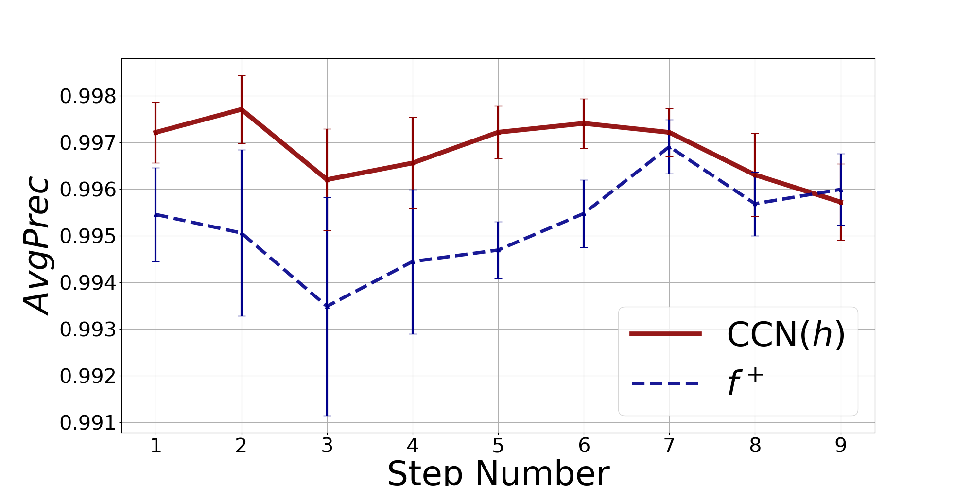
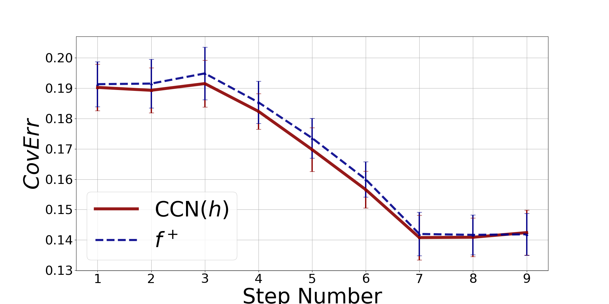
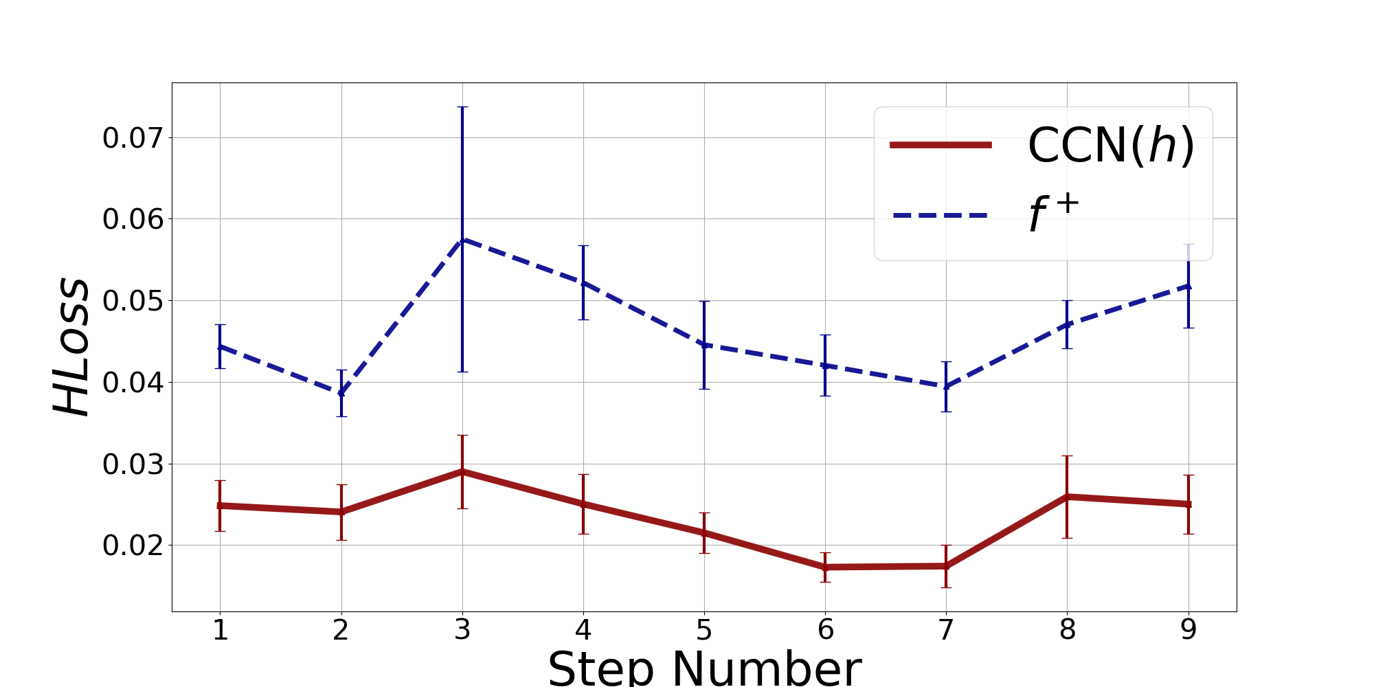
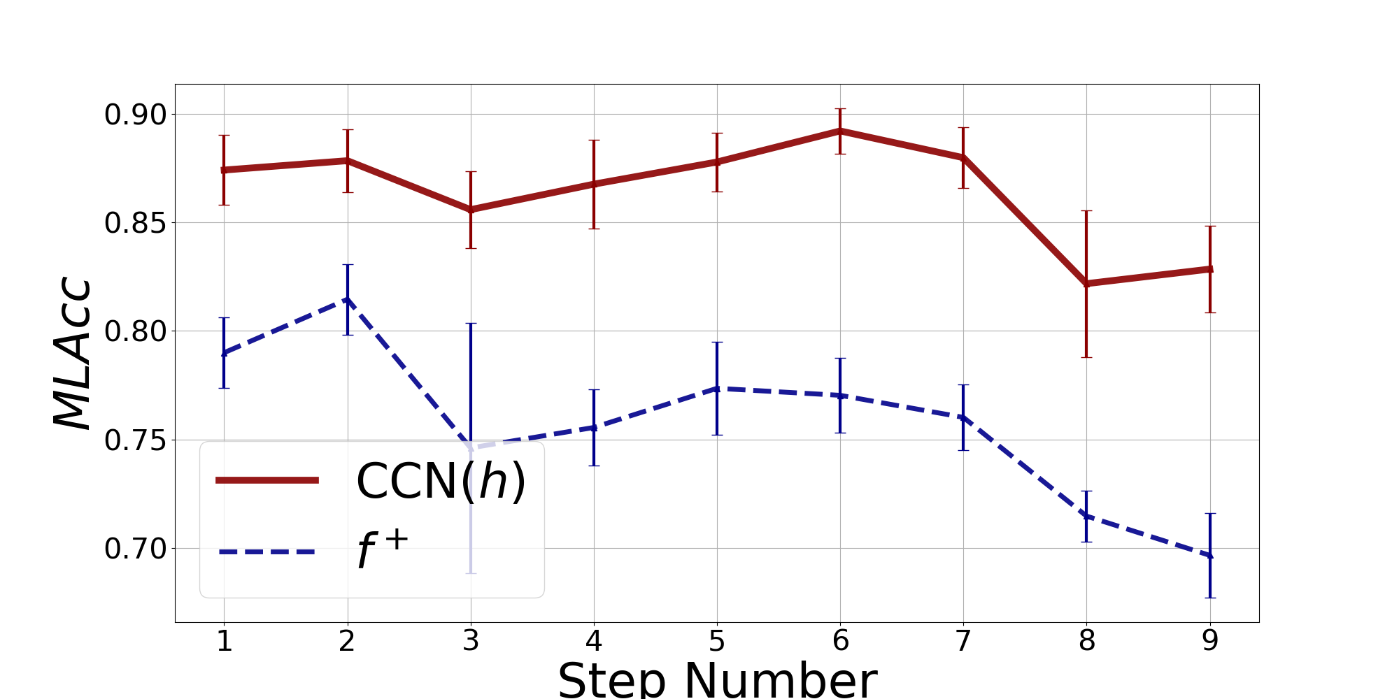
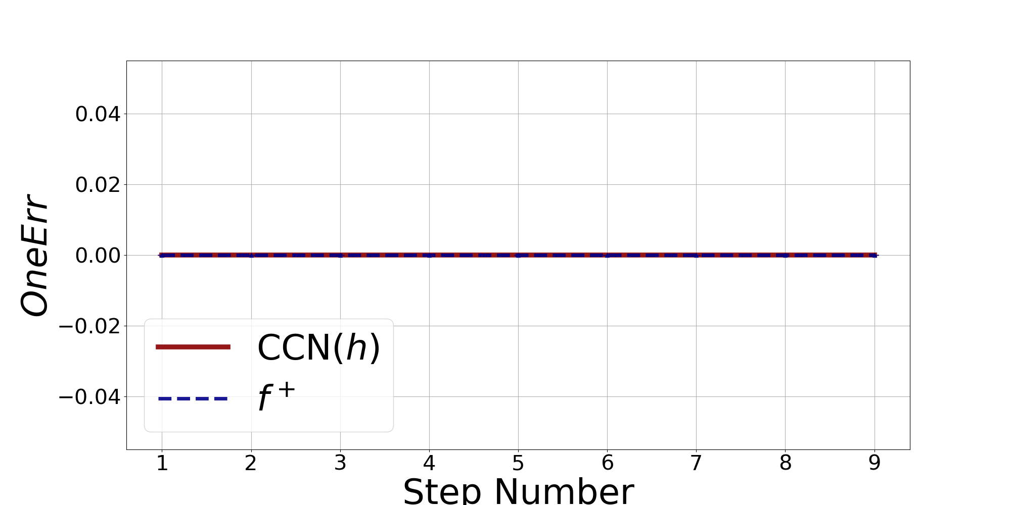
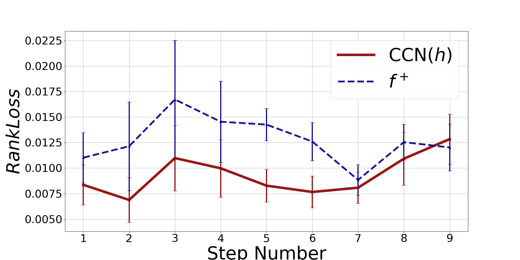
Figure 10: Mean average precision, coverage error, hamming loss, multi-label accuracy, one-error, and ranking loss with standard deviation of CCN($h$) and $f^{+}$ for each step.

5.2.1 Synthetic Experiment

Consider the generalization of the experiment presented as basic case, in which we started with $R_{1}$ outside $R_{2}$ (as in the first row of Fig. 3), and then moved $R_{1}$ towards the centre of $R_{2}$ (as in the second row of Fig. 3) in 9 uniform steps. As for HMC problems, this experiment is meant to show how the performance of CCN($h$) and $f^{+}$ defined as in Section 3.2 vary depending on the relative positions of $R_{1}$ and $R_{2}$. As expected, Figure 10 shows that CCN($h$) performs better or equally to $f^{+}$ at all steps and for all metrics. In particular:

• CCN($h$) performs consistently better than $f^{+}$ at all steps in terms of average precision, coverage error, Hamming loss, multi-label accuracy and ranking loss. Further, as in the HMC case, CCN($h$) exhibits much more stable performances than $f^{+}$ as highlighted by the visibly much smaller standard deviation bar of CCN($h$).

• CCN($h$) and $f^{+}$ perform identically in terms of one-error. This is due to the fact that one-error measures the fraction of instances whose most confident class is irrelevant, since neither CCN($h$) nor $f^{+}$ ever make this mistake, they both have one-error equal to zero at all steps.

Dataset	$D$	$L$	Train	Val	Test	$C$	$H$	$B$	$B^{+}$	$B^{-}$	$H/L$
Arts	462	26	2975	525	1500	344	11	7.1	5.6	1.5	42.3%
Business	438	30	2975	525	1500	77	7	2.5	2.3	0.2	23.3%
Cal500	68	174	298	53	151	39	7	2	1.1	0.9	4.0%
Emotions	72	6	332	59	202	1	1	5	0	5	16.7%
Enron	1001	53	954	169	579	7	5	1	1	0	9.4%
Genbase	1186	27	393	70	199	88	13	2.2	2.0	0.2	48.1%
Image	294	5	1190	210	600	1	1	4	0	4	20.0%
Medical	1449	45	283	50	645	17	9	1.2	1.2	0	20.0%
Rcv1subset1	944	101	3570	630	1800	247	16	3.7	2.9	0.8	15.8%
Rcv1subset2	944	101	3570	630	1800	81	15	2.4	1.7	0.7	14.9%
Rcv1subset3	944	101	3570	630	1800	72	16	2.3	1.7	0.6	15.8%
Rcv1subset4	944	101	3570	630	1800	63	14	2.1	1.7	0.4	13.9%
Rcv1subset5	944	101	3570	630	1800	73	11	2.5	2	0.5	10.9%
Science	743	40	2975	525	1500	37	11	2.1	1.7	0.4	27.5%
Scene	294	6	1029	182	1196	1	1	5	0	5	16.7%
Yeast	103	14	1275	225	917	34	11	2.3	1.9	0.4	78.6%

Table 4: Summary of the real-world MC datasets. For each dataset, we report from left to right: (i) name, (ii) number of features ($D$), (iii) number of classes ($L$), (iv-vi) number of data points for each split, (vii) number of constraints ($C$), (iix) number of different classes that appear at least once as head of a constraint ($H$), (ix) average number of classes appearing in the body ($B$), (x-xi) average number of classes appearing positively (resp., negatively) in the body ($B^{+}$), (resp., ($B^{-}$)), and (xii) percentage of classes appearing at least once as head of a constraint.

Model	Arts	Business	Cal500	Emotions	Enron	Genbase	Image	Medical
	Average precision ($\uparrow$)
CCN($h$)	0.623	0.904	0.520	0.800	0.704	0.996	0.807	0.866
CAMEL	0.625	0.899	0.513	0.756	0.708	0.990	0.793	0.807
ECC	0.544	0.867	0.401	0.772	0.643	1.000	0.738	0.823
BR	0.546	0.863	0.441	0.793	0.643	1.000	0.726	0.823
RAKEL	0.530	0.856	0.433	0.798	0.636	1.000	0.721	0.811
	Coverage error $(\downarrow)$
CCN($h$)	0.172	0.065	0.734	0.315	0.217	0.016	0.187	0.035
CAMEL	0.202	0.083	0.791	0.372	0.256	0.010	0.201	0.036
ECC	0.223	0.089	0.853	0.338	0.285	0.009	0.242	0.045
BR	0.217	0.086	0.789	0.324	0.288	0.009	0.245	0.045
RAKEL	0.221	0.085	0.791	0.317	0.294	0.009	0.250	0.049
	Hamming loss ($\downarrow$)
CCN($h$)	0.054	0.023	0.136	0.197	0.046	0.001	0.172	0.013
CAMEL	0.055	0.023	0.138	0.265	0.047	0.003	0.174	0.024
ECC	0.081	0.031	0.172	0.245	0.055	0.001	0.218	0.019
BR	0.079	0.032	0.162	0.229	0.054	0.001	0.232	0.019
RAKEL	0.082	0.034	0.165	0.223	0.055	0.001	0.225	0.019
	Multi-label accuracy ($\uparrow$)
CCN($h$)	0.238	0.601	0.203	0.534	0.395	0.986	0.488	0.589
CAMEL	0.218	0.609	0.210	0.354	0.381	0.943	0.456	0.284
ECC	0.217	0.548	0.220	0.446	0.361	0.992	0.387	0.481
BR	0.217	0.538	0.221	0.465	0.365	0.992	0.369	0.477
RAKEL	0.215	0.527	0.222	0.485	0.361	0.992	0.376	0.481
	One-error ($\downarrow$)
CCN($h$)	0.475	0.093	0.113	0.273	0.235	0.000	0.296	0.181
CAMEL	0.460	0.090	0.133	0.381	0.223	0.020	0.310	0.285
ECC	0.568	0.137	0.378	0.332	0.309	0.000	0.392	0.251
BR	0.567	0.147	0.232	0.292	0.299	0.000	0.425	0.251
RAKEL	0.586	0.159	0.232	0.292	0.304	0.000	0.430	0.266
	Ranking loss ($\downarrow$)
CCN($h$)	0.115	0.030	0.173	0.161	0.076	0.003	0.159	0.024
CAMEL	0.136	0.040	0.189	0.237	0.086	0.001	0.177	0.026
ECC	0.158	0.046	0.257	0.193	0.107	0.001	0.231	0.033
BR	0.155	0.045	0.218	0.177	0.108	0.001	0.234	0.032
RAKEL	0.159	0.044	0.220	0.169	0.112	0.001	0.242	0.037

Table 5: Comparison of CCN($h$) with the other state-of-the-art models. The best results are in bold.

Model	Rcv1S1	Rcv1S2	Rcv1S3	Rcv1S4	Rcv1S5	Science	Scene	Yeast
	Average precision ($\uparrow$)
CCN($h$)	0.642	0.666	0.647	0.675	0.560	0.603	0.868	0.768
CAMEL	0.622	0.647	0.636	0.654	0.564	0.614	0.824	0.766
ECC	0.549	0.575	0.585	0.609	0.529	0.502	0.794	0.724
BR	0.536	0.563	0.572	0.600	0.524	0.500	0.781	0.743
RAKEL	0.532	0.556	0.562	0.589	0.508	0.493	0.794	0.732
	Coverage error ($\downarrow$)
CCN($h$)	0.092	0.089	0.103	0.080	0.107	0.131	0.077	0.452
CAMEL	0.131	0.115	0.123	0.103	0.130	0.162	0.106	0.457
ECC	0.185	0.166	0.167	0.169	0.196	0.225	0.127	0.495
BR	0.194	0.181	0.178	0.184	0.210	0.227	0.128	0.476
RAKEL	0.201	0.180	0.185	0.195	0.209	0.225	0.123	0.481
	Hamming loss ($\downarrow$)
CCN($h$)	0.026	0.022	0.024	0.019	0.025	0.031	0.092	0.196
CAMEL	0.027	0.022	0.024	0.021	0.025	0.031	0.109	0.196
ECC	0.031	0.027	0.028	0.026	0.030	0.049	0.131	0.221
BR	0.032	0.028	0.029	0.027	0.031	0.051	0.151	0.214
RAKEL	0.033	0.029	0.030	0.027	0.031	0.051	0.130	0.225
	Multi-label accuracy ($\uparrow$)
CCN($h$)	0.296	0.310	0.303	0.324	0.275	0.255	0.607	0.480
CAMEL	0.204	0.222	0.210	0.257	0.223	0.217	0.528	0.480
ECC	0.264	0.277	0.273	0.297	0.269	0.209	0.478	0.443
BR	0.263	0.279	0.275	0.289	0.263	0.200	0.438	0.456
RAKEL	0.263	0.272	0.268	0.290	0.258	0.201	0.481	0.445
	One-error ($\downarrow$)
CCN($h$)	0.413	0.389	0.405	0.379	0.402	0.494	0.224	0.234
CAMEL	0.413	0.397	0.413	0.399	0.414	0.472	0.287	0.231
ECC	0.477	0.462	0.453	0.436	0.451	0.603	0.319	0.300
BR	0.492	0.474	0.466	0.435	0.466	0.605	0.358	0.259
RAKEL	0.488	0.481	0.471	0.439	0.474	0.606	0.329	0.270
	Ranking loss ($\downarrow$)
CCN($h$)	0.036	0.035	0.046	0.035	0.046	0.094	0.073	0.172
CAMEL	0.051	0.048	0.050	0.046	0.054	0.117	0.101	0.173
ECC	0.086	0.078	0.078	0.086	0.093	0.176	0.103	0.208
BR	0.091	0.088	0.085	0.097	0.101	0.177	0.131	0.190
RAKEL	0.093	0.088	0.089	0.103	0.102	0.180	0.127	0.200

Table 6: Comparison of CCN($h$) with the other state-of-the-art models. The best results are in bold.

Metric	Average ranking					Friedman test	Wilcoxon test
	CCN($h$)	CAMEL	ECC	BR	RAKEL	p-value	CCN($h$) vs. CAMEL
Average precision	1.43	2.31	3.34	3.56	4.34	$\checkmark\checkmark$	$\checkmark\checkmark$
Coverage Error	1.25	2.41	3.60	3.78	3.94	$\checkmark\checkmark$	$\checkmark\checkmark$
Hamming loss	1.28	2.38	3.38	3.69	4.09	$\checkmark\checkmark$	$\checkmark\checkmark$
Multi-label accuracy	1.53	3.53	3.09	3.38	3.47	$\checkmark\checkmark$	$\checkmark\checkmark$
One-error	1.44	2.22	3.50	3.56	4.28	$\checkmark\checkmark$
Ranking loss	1.25	2.22	3.44	3.69	4.31	$\checkmark\checkmark$	$\checkmark\checkmark$

Table 7: Average ranking for each metric and model, results of the Friedman and Wilcoxon test (the latter deployed to compare the performance of CCN($h$) and CAMEL). We use $\checkmark$ (resp., $\checkmark\checkmark$) to indicate that the test returned p-value $<0.05$ (resp., $<0.01$).

5.3 Comparison with the State of the Art

In order to prove the superiority of our model, we adopted the same methodology presented in (?) and consider the three well-established MC models and the state-of-the-art MC model tested in  (?), which can be characterized by the order of classes correlations they exploit. Thus, CCN($h$) is compared with

1. BR (?), a first order model which considers each class separately, ignoring class correlations, and

2. ECC (?), RAKEL (?) and CAMEL (?), which exploit correlations among two or more classes.

BR, ECC, and RAKEL are the well-established MC models, and CAMEL is the current state-of-the-art MC model (?). Since these models are not guaranteed to output predictions that are coherent with the constraints, we applied CM as additional post-processing steps.

Being the first paper on LCMC problems, we created 16 real-world LCMC datasets, each obtained by enriching a popular and publicly available MC dataset with constraints extracted using the apriori algorithm (?). The list of the datasets together with a summary of their characteristics is reported in Table 4. The various datasets come from different application domains, in particular:

1. Cal500 and Emotions are 2 music classification datasets (?, ?),

2. Genbase and Yeast are 2 functional genomics datasets (?, ?),

3. Image and Scene are 2 image classification datasets (?, ?), and

4. the remaining 10 are text classification datasets (?, ?, ?, ?).

Furthermore, as it can be seen from Table 4, they differ significantly both in the number of data points/classes (columns $D$ and $L$) and in the characteristics of the associated sets of constraints. Indeed, we have datasets having just a few (one)/many constraints (column $C$), involving a few/many classes in the head (column $H/L$) and in the body, either positively or negatively (columns $B$, $B^{+}$ and $B^{-}$).

As in the HMC experiments, we applied the same preprocessing to all the datasets. All the categorical features were transformed using one-hot encoding. The missing values were replaced by their mean in the case of numeric features and by a vector of all zeros in the case of categorical ones. All the features were standardized. As in the HMC experiments, we built $h$ as a feedforward neural network with two hidden layers and ReLU non-linearity. To prove the robustness of CCN($h$), we kept all the hyperparameters fixed except the hidden dimension used for each dataset, which is given in Appendix B. Such hidden dimensions were optimized over the validation sets. In all experiments, the loss was minimized using Adam optimizer with batch size equal to 4, learning rate equal to $10^{-4}$, and patience $20$ ($\beta_{1}=0.9,\beta_{2}=0.999$). Since some datasets have very few data points, we set the dropout rate equal to $80\%$ and the weight decay equal to $10^{-4}$. As for the HMC case, we retrained CCN($h$) on both training and validation data for the same number of epochs, as the early stopping procedure determined was optimal in the first pass. For each dataset, we run the models 10 times, and the average for each of the metrics is reported in Tables 5 and 6. For ease of presentation, we omit the standard deviations, which for CCN($h$) are in the range $[2.9\times 10^{-17},8.0\times 10^{-3}]$, proving that it is a very stable model. ECC, BR, and RAKEL were implemented using scikit-multilearn (?) by deploying the logistic regression model as the base classifier. Regarding CAMEL, we used the publicly available authors’ implementation, with the hyperparameters suggested by the authors. For all the models, we got results comparable to the ones reported in (?).

As it can be seen in Tables 5 and 6, CCN($h$) has the highest number of wins in all metrics. Indeed, as it can be seen in Table 7, CCN($h$) has the best average ranking in all metrics. We also verified the statistical significance of the results following (?) by performing the Friedman test for each metric. As reported in Table 7, the Friedman test returned p-value $<0.01$ for each metric; we could thus proceed with the post-hoc Nemenyi tests, and the resulting critical diagrams are reported in Figure 11. In each diagram, the groups of methods that do not differ significantly (significance level 0.05) are connected through an horizontal line. According to the Nemenyi test, CCN($h$)’s performance differs significantly to the performance of all the other models but CAMEL in terms of average precision, coverage error, Hamming loss, one-error and ranking loss, while it differs significantly to all the models (including CAMEL) in terms of multi-label accuracy. As in the HMC case, we then followed the guidelines given in (?, ?) and performed the Wilcoxon test to compare the difference between CAMEL and CCN($h$). As reported in the last column of Table 7, the performances of CCN($h$) and CAMEL differ significantly for all metrics but one-error, thus further confirming the superiority of our model.

(a) Average precision

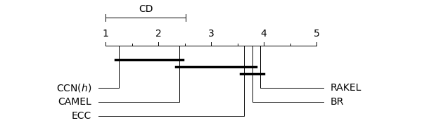
(b) Coverage error

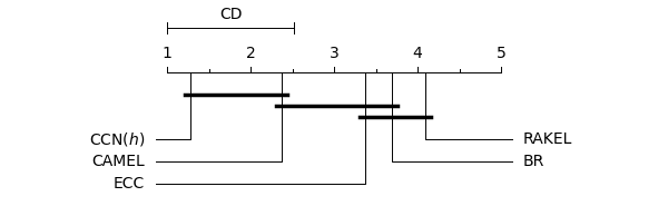
(c) Hamming loss

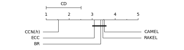
(d) Multi-label accuracy

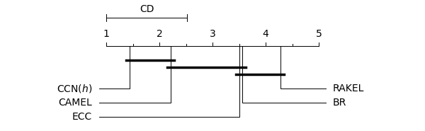
(e) One-error

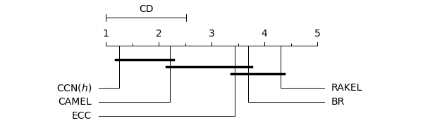
(f) Ranking loss

Figure 11: Critical diagram for each metric obtained with the post-hoc Nemenyi test.

Model	Arts	Business	Cal500	Emotions	Enron	Genbase	Image	Medical
	Average precision ($\uparrow$)
CCN($h$)	0.623	0.904	0.520	0.800	0.704	0.996	0.807	0.866
$h^{+}$	0.623	0.903	0.519	0.796	0.704	0.996	0.800	0.868
$h$+CM	0.623	0.902	0.519	0.800	0.704	0.978	0.807	0.864
	Coverage error ($\downarrow$)
CCN($h$)	0.172	0.065	0.734	0.315	0.217	0.016	0.187	0.035
$h^{+}$	0.172	0.073	0.734	0.319	0.217	0.017	0.194	0.037
$h$+CM	0.173	0.072	0.734	0.311	0.217	0.020	0.187	0.037
	Hamming loss ($\downarrow$)
CCN($h$)	0.054	0.023	0.136	0.197	0.046	0.001	0.172	0.013
$h^{+}$	0.054	0.026	0.136	0.201	0.046	0.001	0.172	0.015
$h$+CM	0.054	0.026	0.136	0.198	0.046	0.003	0.169	0.015
	Multi-label accuracy ($\uparrow$)
CCN($h$)	0.238	0.601	0.203	0.534	0.395	0.986	0.488	0.589
$h^{+}$	0.238	0.601	0.203	0.512	0.395	0.986	0.475	0.591
$h$+CM	0.237	0.599	0.203	0.519	0.395	0.935	0.487	0.587
	One-error ($\downarrow$)
CCN($h$)	0.475	0.093	0.113	0.273	0.235	0.000	0.296	0.181
$h^{+}$	0.476	0.093	0.113	0.283	0.238	0.000	0.307	0.181
$h$+CM	0.475	0.093	0.113	0.276	0.237	0.004	0.297	0.185
	Ranking loss ($\downarrow$)
CCN($h$)	0.115	0.030	0.173	0.161	0.076	0.003	0.159	0.024
$h^{+}$	0.116	0.034	0.173	0.167	0.076	0.003	0.169	0.026
$h$+CM	0.116	0.034	0.173	0.159	0.076	0.006	0.160	0.025

Table 8: Results of the ablations studies. The best results are in bold.

Model	Rcv1S1	Rcv1S2	Rcv1S3	Rcv1S4	Rcv1S5	Science	Scene	Yeast
	Average precision ($\uparrow$)
CCN($h$)	0.642	0.666	0.647	0.675	0.560	0.603	0.868	0.768
$h^{+}$	0.639	0.662	0.645	0.663	0.548	0.603	0.864	0.765
$h$+CM	0.630	0.663	0.640	0.682	0.560	0.602	0.867	0.767
	Coverage error ($\downarrow$)
CCN($h$)	0.092	0.089	0.103	0.080	0.107	0.131	0.077	0.452
$h^{+}$	0.093	0.090	0.102	0.089	0.112	0.135	0.081	0.455
$h$+CM	0.092	0.090	0.103	0.089	0.115	0.135	0.078	0.453
	Hamming loss ($\downarrow$)
CCN($h$)	0.026	0.022	0.024	0.019	0.025	0.031	0.092	0.196
$h^{+}$	0.027	0.023	0.025	0.022	0.027	0.032	0.092	0.196
$h$+CM	0.027	0.023	0.025	0.020	0.025	0.032	0.092	0.196
	Multi-label accuracy ($\uparrow$)
CCN($h$)	0.296	0.310	0.303	0.324	0.275	0.255	0.607	0.480
$h^{+}$	0.296	0.309	0.305	0.323	0.277	0.257	0.603	0.487
$h$+CM	0.283	0.306	0.301	0.321	0.257	0.250	0.604	0.482
	One-error ($\downarrow$)
CCN($h$)	0.413	0.389	0.405	0.379	0.402	0.494	0.224	0.234
$h^{+}$	0.413	0.396	0.405	0.394	0.420	0.494	0.227	0.234
$h$+CM	0.434	0.391	0.407	0.357	0.407	0.496	0.226	0.231
	Ranking loss ($\downarrow$)
CCN($h$)	0.036	0.035	0.046	0.035	0.046	0.094	0.073	0.172
$h^{+}$	0.036	0.036	0.046	0.039	0.049	0.097	0.077	0.172
$h$+CM	0.037	0.037	0.047	0.039	0.049	0.096	0.074	0.174

Table 9: Results of the ablation studies. The best results are in bold.

Metric	Average ranking			Wilcoxon test
	CCN($h$)	$h^{+}$	$h$+CM	CCN($h$) vs. $h^{+}$	CCN($h$) vs. $h$+CM
Average precision	1.41	2.34	2.25	$\checkmark\checkmark$	$\checkmark$
Coverage error	1.38	2.41	2.22	$\checkmark\checkmark$	$\checkmark$
Hamming loss	1.47	2.38	2.16	$\checkmark\checkmark$	$\checkmark$
Multi-label accuracy	1.63	1.75	2.63		$\checkmark\checkmark$
One-error	1.47	2.38	2.16	$\checkmark$
Ranking loss	1.31	2.31	2.38	$\checkmark\checkmark$	$\checkmark\checkmark$

Table 10: Average ranking for each metric and model, and results of the Wilcoxon test: $\checkmark$ (resp., $\checkmark\checkmark$) is used to indicate that the Wilcoxon test returned p-value $<0.05$ (resp., $<0.01$).

5.4 Ablation Studies

As in the HMC case, in order to analyze the impact of both CM and CLoss, we compared the performance of CCN($h$) against the performance of $h^{+}$, i.e., $h$ with the enforcement of the constraints done as a post-processing step, and $h+\text{\rm CM}$, i.e., $h$ with CM built on top. Both these models were trained using the standard binary cross-entropy loss. The results of the ablation studies for each metric and each dataset are given in Tables 8 and 9, while the average ranking for each metric can be found in Table 10. As it can be seen in Table 10, CCN($h$) has the highest average ranking for all metrics. Furthermore, we check the statistical significance of our results through the Wilcoxon test, whose results are reported in the last two columns of Table 10. As it can be seen, CCN($h$) performs significantly better than $h^{+}$ for all metrics but multi-label accuracy. On the other hand, CCN($h$) performs significantly better than $h+\text{\rm CM}$ for all metrics but one-error.

6 Related Work

In this paper, we introduced LCMC problems, i.e., MC problems in which every prediction must satisfy a given set of hard constraints expressed as normal rules. HMC problems are special cases of LCMC in which the body of each constraint is a single class and with the additional restriction that the constraint graph associated to the set of constraints is acyclic.

We divide this section on the related work into two parts: in the first part, we focus on the literature in the HMC field, while in the second part, we present and discuss the previous works that have already dealt with the problem of imposing more expressive constraints on MC problems.

6.1 Hierarchical Multi-Label Classification

In the literature, HMC methods are traditionally divided into local and global approaches (?).

Local approaches decompose the problem into smaller classification ones, and then the solutions are combined to solve the main task. Local approaches can be further divided based on the strategy that they deploy to decompose the main task. If a method trains a different classifier for each level of the hierarchy, then we have a local classifier per level, as in (?, ?, ?, ?, ?). The works (?, ?, ?) are extended by ? (?), where HMCN-R and HMCN-F are presented. Since HMCN-R and HMCN-F are trained with both a local loss and a global loss, they are considered hybrid local-global approaches. If a method trains a classifier for each node of the hierarchy, then we have a local classifier per node. In (?), a linear classifier is trained for each node with a loss function that captures the hierarchy structure. On the other hand, in (?), one multi-layer perceptron for each node is deployed. A different approach is proposed in (?), where kernel dependency estimation is employed to project each class to a low-dimensional vector. To preserve the hierarchy structure, a generalized condensing sort and select algorithm is developed, and each vector is then learned singularly using ridge regression. Finally, if a method trains a different classifier per parent node in the hierarchy, then we have a local classifier per parent node. For example, ? (?) propose to train a model for each sub-ontology of the Gene Ontology, combining features automatically learned from the sequences and features based on protein interactions. ? (?), instead, try to solve the overfitting problem typical of local models by representing the correlation among the classes by the class distribution, and then training each local model to map data points to class distributions.

Global methods consist of single models able to map objects with their corresponding classes in the hierarchy as a whole. A well-known global method is Clus-HMC (?), consisting of a single predictive clustering tree for the entire hierarchy. This work is extended by ? (?), who propose Clus-Ens: an ensemble of Clus-HMC. In (?), a neural network incorporating the structure of the hierarchy in its architecture is proposed. While this network makes predictions that are coherent with the hierarchy, it also makes the assumption that each parent class is the union of the children. ? (?) propose competitive neural networks, whose architecture replicates the hierarchy. The name of these networks comes from the fact that the neurons in the output layer compete with each other to be activated.

If we move the focus on how the satisfaction of the constraints is guaranteed, HMC models can be divided in:

1. approaches that satisfy the constraints by construction, and

2. approaches that require a post-processing step to enforce the constraints.

In the first category, we can find methods such as Clus-HMC (?), in which each constraint $A_{1}\to A$ is satisfied by properly setting the thresholds for both $A$ and $A_{1}$. Clus-Ens, the ensemble of Clus-HMC, computes the average of all class vectors predicted by the trees in the ensemble and then applies the threshold mechanism of Clus-HMC. In this way, its predictions always satisfy the constraints. The model proposed in (?), in order to preserve the hierarchy structure, develops a generalized condensing sort and select algorithm, while ? (?) evaluate the node classifiers in a top-down fashion, thus not making a prediction at all for the descendants of a node that has not been predicted.

Many of the neural-network-based models belong to the second category. A common policy to enforce the satisfaction of $A_{1}\to A$ is to force the output for class $A_{1}$ to be smaller than or equal to the output for $A$ (see, e.g., (?, ?, ?, ?)). However, other solutions are possible. For example, ? (?) associate to each data point an initial set of classes which is then extended to include all their ancestors in the hierarchy, while ? (?) apply a post processing method based on Bayesian networks in order to guarantee that the results are coherent with the hierarchy constraints. For a detailed overview on the many different policies that can be used to impose the hierarchy constraints as a post-processing step, see (?).

6.2 More expressive constraints

When dealing with more expressive constraints, researchers have mostly focused on the problem of exploiting them to improve their models and/or to deal with data scarcity, curiously neglecting the problem of guaranteeing their satisfaction.

If we focus on constraints expressed as logic rules, then we can find works such as (?), in which the authors introduce an iterative method to embed structured information expressed by first order logic (FOL) formulas into the weights of different kinds of deep neural networks. At each step, they consider a teacher network based on the set of FOL rules to train a student network to fit both supervisions and logic rules. The work has been later extended to jointly learn the structure of the rules and their weights (?). A different approach is considered in (?), where a new framework is introduced to augment a neural network assigning semantics via logical rules to its neurons. Indeed, some neurons are associated with logical predicates, and then their activation is modified depending on the activation of the neurons corresponding to predicates that co-occur in the same rules. Many works embed logical constraints into penalty functions to formulate a learning problem, see e.g., (?, ?, ?). These works generally consider a fuzzy relaxation of FOL formulas to get a differentiable loss function that may be minimized by gradient descent. However, as the loss function is minimized, there is no guarantee that the constraints are fully satisfied.

If we further broaden our view to more general constraints, i.e., to any constraint that enforces some correlation on the outputs of the model, then we can find a very wide literature, in which many works have shown that exploiting the background knowledge expressed by the constraints can bring some benefits. For example, ? (?) exploit the background knowledge coming from known laws of physics to train neural networks without any labeled example. ? (?) combine Markov random fields with deep neural networks to express some context correlation in an image segmentation task. Similarly, ? (?) consider conditional random fields on top of a bidirectional LSTM (?) to enforce some statistical co-occurrencies (n-grams) among the network predictions, achieving state-of-the-art performance on POS and chunking tasks. Some of these works have also tried to impose hard constraints on learning algorithms, however, dealing effectively with hard constraints commonly requires a specific optimization schema, e.g., by considering a sequence of problems where the hard constraints are replaced by soft ones associated with larger and larger penalties, (see (?, ?) for a detailed dissertation on optimization methods), and convergence is only guaranteed under suitable conditions; see (?). ? (?) consider different learning problems where both soft and hard constraints are taken into account at the same time. Soft constraints are added to the penalty function, while the optimal solution (if it exists) is required to satisfy a system of (in)equalities corresponding to the hard constraints. A newly devised approach to asymptotically satisfy hard constraints is considered in (?), where the authors use the distributed asynchronous method of multipliers to solve the optimization problem.

7 Conclusion

In this paper, we introduced and dealt with LCMC problems, i.e., on MC problems with hard constraints expressed as normal logic rules. We first focused on the special case represented by HMC problems, and proposed C-HMCNN($h$), a novel model based on neural networks that (i) is able to leverage the hierarchical information to learn when to delegate the prediction on a superclass to one of its subclasses, (ii) produces predictions coherent by construction, and (iii) outperforms current state-of-the-art models on 20 commonly used real-world HMC benchmarks, and (iv) it can be easily implemented on GPUs using standard libraries. We then considered the general case and proposed CCN($h$), which has four distinguishing features: (i) its predictions are always coherent with the given constraints, (ii) it can be implemented on GPUs using standard libraries, (iii) it extends C-HMCNN($h$), and thus outperforms the state-of-the-art HMC models on HMC problems, and (iv) it outperforms the state-of-the-art MC models on 16 LCMC problems obtained adding automatically extracted constraints to well-known MC problems.

This work opens the path to many different lines of research. In general, the basic idea behind this paper is to (i) incorporate the constraints in neural networks models guaranteeing their coherency, and (ii) exploit the constraints to improve performance. In this paper, we focussed on MC problems with hard logical constraints on the output, but indeed the same idea can be applied also to other problems, and it could be interesting to investigate (i) whether it is possible to impose even more expressive constraints (e.g., involving also the input), (ii) how to incorporate both soft and hard constraints, and (iii) how to impose hard constraints on regression, binary classification, and multi-class classification problems.

Acknowledgments

This paper is a revised and substantially extended version of the paper (?). We thank Lei Feng, Francesco Giannini and Marco Gori for useful discussions. Eleonora Giunchiglia is supported by the EPSRC under the grant EP/N509711/1 and by an Oxford-DeepMind Graduate Scholarship. This work was also supported by the Alan Turing Institute under the EPSRC grant EP/N510129/1 and by the AXA Research Fund. We also acknowledge the use of the EPSRC-funded Tier 2 facility JADE (EP/P020275/1) and GPU computing support by Scan Computers International Ltd.

A HMC - Experimental Analysis Details

Dataset	Hidden Dimension	Learning Rate	Time per batch (ms)
Cellcycle FUN	500	$10^{-4}$	2.0
Derisi FUN	500	$10^{-4}$	2.0
Eisen FUN	500	$10^{-4}$	1.7
Expr FUN	1000	$10^{-4}$	1.9
Gasch1 FUN	1000	$10^{-4}$	2.0
Gasch2 FUN	500	$10^{-4}$	2.8
Seq FUN	2000	$10^{-4}$	2.0
Spo FUN	250	$10^{-4}$	1.6
Cellcycle GO	1000	$10^{-4}$	2.4
Derisi GO	500	$10^{-4}$	2.5
Eisen GO	500	$10^{-4}$	3.4
Expr GO	4000	$10^{-5}$	3.9
Gasch1 GO	500	$10^{-4}$	2.5
Gasch2 GO	500	$10^{-4}$	2.8
Seq GO	9000	$10^{-5}$	2.6
Spo GO	500	$10^{-4}$	3.3
Diatoms	2000	$10^{-5}$	2.0
Enron	1000	$10^{-5}$	3.6
Imclef07a	1000	$10^{-5}$	3.4
Imclef07d	1000	$10^{-5}$	2.9

Table 11: Hidden dimension used for each dataset, learning rate used for each dataset, and average inference time per batch in milliseconds (ms). Average computed over 500 batches for each dataset.

In this section, we provide more details about the conducted experimental analysis for HMC problems. As stated in the paper, across the different experiments, we kept all hyperparameters fixed with the exception of the hidden dimension and the learning rate, which are reported in the first two columns of Table 11. The other hyperparameters were determined by searching the best hyperparameters configuration on the Funcat datasets; we then took the configuration that led to the best results on the highest number of datasets. The hyperparameter values taken in consideration were: (i) learning rate: $[10^{-3},10^{-4},10^{-5}]$, (ii) batch size: $[4,64,256]$, (iii) dropout: $[0.6,0.7]$, and (iv) weight decay: $[10^{-3},10^{-5}]$. Concerning the hidden dimension, we took into account all possible dimensions from 250 to 2000 with step equal to 250, and from 2000 to 10000 with step 1000. The last column of Table 11 shows the average inference time per batch in milliseconds. The average is computed over 500 batches for each dataset. All experiments were run on an Nvidia Titan Xp with 12 GB memory.

B LCMC - Experimental Analysis Details

Dataset	Hidden Dimension
Arts	4000
Business	4000
Cal500	100
Emotions	100
Enron	2500
Genbase	5000
Image	1000
Medical	800
Rcv1Subset1	600
Rcv1Subset2	1500
Rcv1Subset3	4000
Rcv1Subset4	1000
Rcv1Subset5	4000
Science	2000
Scene	1500
Yeast	4000

Table 12: Hidden dimension used for each dataset.

In this section, we provide more details about the conducted experimental analysis for LCMC problems. As stated in the paper, across the different experiments, we kept all hyperparameters fixed with the exception of the hidden dimension, which are reported in Table 12. The other hyperparameters were determined by searching the best hyperparameters configuration on the validation sets; we then took the configuration that led to the best results on the highest number of datasets. The hyperparameter values taken in consideration were: (i) learning rate: $[10^{-3},10^{-4},10^{-5}]$, (ii) batch size: $[4,64,256]$, (iii) dropout: $[0.6,0.7,0.8]$, and (iv) weight decay: $[10^{-3},10^{-4},10^{-5}]$. Concerning the hidden dimension, we took into account all possible dimensions from 100 to 1000 with step equal to 100, and from 1000 to 5000 with step 500. Again, all experiments were run on an Nvidia Titan Xp with 12 GB memory.

References

- Agrawal and Srikant Agrawal, R., and Srikant, R. (1994). Fast algorithms for mining association rules in large databases. In Proceedings of VLDB, pp. 487–499.
- Apt et al. Apt, K. R., Blair, H. A., and Walker, A. (1988). Towards a theory of declarative knowledge. In Minker, J. (Ed.), Foundations of Deductive Databases and Logic Programming, pp. 89–148. Morgan Kaufmann.
- Barutcuoglu et al. Barutcuoglu, Z., Schapire, R. E., and Troyanskaya, O. G. (2006). Hierarchical multi-label prediction of gene function. Bioinformatics, 22(7), 830–836.
- Benavoli et al. Benavoli, A., Corani, G., and Mangili, F. (2016). Should we really use post-hoc tests based on mean-ranks?. Journal of Machine Learning Research, 17(5), 1–10.
- Bertsekas Bertsekas, D. P. (2014). Constrained Optimization and Lagrange Multiplier Methods. Academic Press.
- Bi and Kwok Bi, W., and Kwok, J. T. (2011). Multi-label classification on tree- and DAG-structured hierarchies. In Proceedings of ICML, pp. 17–24.
- Borges and Nievola Borges, H. B., and Nievola, J. C. (2012). Multi-label hierarchical classification using a competitive neural network for protein function prediction. In Proceedings of IJCNN, pp. 1–8.
- Boutell et al. Boutell, M. R., Luo, J., Shen, X., and Brown, C. M. (2004). Learning multi-label scene classification. Pattern Recognition, 37(9).
- Cerri et al. Cerri, R., Barros, R. C., and de Leon Ferreira de Carvalho, A. C. P. (2011). Hierarchical multi-label classification for protein function prediction: A local approach based on neural networks. In Proceedings of ISDA, pp. 337–343.
- Cerri et al. Cerri, R., Barros, R. C., and de Leon Ferreira de Carvalho, A. C. P. (2014). Hierarchical multi-label classification using local neural networks. Journal of Computer and System Sciences, 80(1), 39–56.
- Cerri et al. Cerri, R., Barros, R. C., de Leon Ferreira de Carvalho, A. C. P., and Jin, Y. (2016). Reduction strategies for hierarchical multi-label classification in protein function prediction. BMC Bioinformatics, 17, 373.
- Cesa-Bianchi et al. Cesa-Bianchi, N., Gentile, C., and Zaniboni, L. (2006). Incremental algorithms for hierarchical classification. Journal of Machine Learning Research, 7, 31–54.
- Chen et al. Chen, L.-C., Schwing, A., Yuille, A., and Urtasun, R. (2015). Learning deep structured models. In Proceedings of ICML, pp. 1785–1794.
- Clare Clare, A. (2003). Machine Learning and Data Mining for Yeast Functional Genomics. Ph.D. thesis, University of Wales.
- Cormen et al. Cormen, T. H., Leiserson, C. E., Rivest, R. L., and Stein, C. (2009). Introduction to Algorithms, 3rd Edition. MIT Press.
- Demsar Demsar, J. (2006). Statistical comparisons of classifiers over multiple data sets. Journal of Machine Learning Research, 7, 1–30.
- Deng et al. Deng, J., Ding, N., Jia, Y., Frome, A., Murphy, K., Bengio, S., Li, Y., Neven, H., and Adam, H. (2014). Large-scale object classification using label relation graphs. In Proceedings of ECCV, Vol. 8689, pp. 48–64.
- Deng et al. Deng, J., Dong, W., Socher, R., Li, L., Li, K., and Li, F. (2009). ImageNet: A large-scale hierarchical image database. In Proceedings of CVPR, pp. 248–255.
- Diligenti et al. Diligenti, M., Gori, M., and Sacca, C. (2017). Semantic-based regularization for learning and inference. Artificial Intelligence, 244, 143–165.
- Dimitrovski et al. Dimitrovski, I., Kocev, D., Loskovska, S., and Džeroski, S. (2008). Hierchical annotation of medical images. In Proceedings of IS, pp. 174–181.
- Dimitrovski et al. Dimitrovski, I., Kocev, D., Loskovska, S., and Dzeroski, S. (2012). Hierarchical classification of diatom images using ensembles of predictive clustering trees. Ecological Informatics, 7(1), 19–29.
- Diplaris et al. Diplaris, S., Tsoumakas, G., Mitkas, P. A., and Vlahavas, I. (2005). Protein classification with multiple algorithms. In Bozanis, P., and Houstis, E. N. (Eds.), Advances in Informatics, pp. 448–456.
- Donadello et al. Donadello, I., Serafini, L., and d’Avila Garcez, A. (2017). Logic tensor networks for semantic image interpretation. In Proceedings of IJCAI, pp. 1596–1602.
- Elisseeff and Weston Elisseeff, A., and Weston, J. (2001). A kernel method for multi-labelled classification. In Proceedings of NeurIPS, p. 681–687.
- Farina et al. Farina, F., Melacci, S., Garulli, A., and Giannitrapani, A. (2020). Asynchronous distributed learning from constraints. IEEE Transactions on Neural Networks and Learning Systems, 31(10), 4367–4373.
- Feng et al. Feng, L., An, B., and He, S. (2019). Collaboration based multi-label learning. In Proceedings of AAAI, pp. 3550–3557.
- Feng et al. Feng, S., Fu, P., and Zheng, W. (2018). A hierarchical multi-label classification method based on neural networks for gene function prediction. Biotechnology and Biotechnological Equipment, 32, 1613–1621.
- Fletcher Fletcher, R. (2013). Practical Methods of Optimization. John Wiley & Sons.
- Gelfond and Lifschitz Gelfond, M., and Lifschitz, V. (1988). The stable model semantics for logic programming. In Logic Programming, Proceedings of the 5th International Conference and Symposium, pp. 1070–1080.
- Giunchiglia and Lukasiewicz Giunchiglia, E., and Lukasiewicz, T. (2020). Coherent hierarchical multi-label classification networks. In Proceedings of NeurIPS, Vancouver, Canada.
- Gnecco et al. Gnecco, G., Gori, M., Melacci, S., and Sanguineti, M. (2014). Learning with mixed hard/soft pointwise constraints. IEEE Transactions on Neural Networks and Learning Systems, 26(9), 2019–2032.
- Hochreiter and Schmidhuber Hochreiter, S., and Schmidhuber, J. (1997). Long short-term memory. Neural Computation, 9(8), 1735–1780.
- Hu et al. Hu, Z., Ma, X., Liu, Z., Hovy, E., and Xing, E. (2016a). Harnessing deep neural networks with logic rules. In Proceedings of ACL, pp. 2410–2420.
- Hu et al. Hu, Z., Yang, Z., Salakhutdinov, R., and Xing, E. (2016b). Deep neural networks with massive learned knowledge. In Proceedings of EMNLP, pp. 1670–1679.
- Huang et al. Huang, X., Kroening, D., Ruan, W., Sharp, J., Sun, Y., Thamo, E., Wu, M., and Yi, X. (2020). A survey of safety and trustworthiness of deep neural networks: Verification, testing, adversarial attack and defence, and interpretability. Computer Science Review, 37, 100270.
- Huang et al. Huang, Z., Xu, W., and Yu, K. (2015). Bidirectional LSTM-CRF models for sequence tagging. ArXiv, abs/1508.01991.
- Kingma and Ba Kingma, D. P., and Ba, J. (2015). Adam: A method for stochastic optimization. In Proceedings of ICLR.
- Klimt and Yang Klimt, B., and Yang, Y. (2004). The Enron Corpus: A new dataset for email classification research. In Proceedings of ECML, pp. 217–226.
- Kulmanov et al. Kulmanov, M., Khan, M. A., and Hoehndorf, R. (2018). DeepGO: Predicting protein functions from sequence and interactions using a deep ontology-aware classifier. Bioinformatics, 34(4), 660–668.
- Lewis et al. Lewis, D. D., Yang, Y., Rose, T. G., and Li, F. (2004). RCV1: A new benchmark collection for text categorization research. Journal of Machine Learning Research, 5, 361–397.
- Li and Srikumar Li, T., and Srikumar, V. (2019). Augmenting neural networks with first-order logic. In Proceedings of ACL, pp. 292–302.
- Li et al. Li, Y., Wang, S., Umarov, R., Xie, B., Fan, M., Li, L., and Gao, X. (2018). DEEPre: Sequence-based enzyme EC number prediction by deep learning. Bioinformatics, 34(5), 760–769.
- Lloyd Lloyd, J. W. (1987). Foundations of Logic Programming, 2nd Edition. Springer.
- Lomuscio and Maganti Lomuscio, A., and Maganti, L. (2017). An approach to reachability analysis for feed-forward relu neural networks. CoRR, abs/1706.07351.
- Luenberger Luenberger, D. G. (1997). Optimization by Vector Space Methods. John Wiley & Sons.
- Ma et al. Ma, L., Juefei-Xu, F., Zhang, F., Sun, J., Xue, M., Li, B., Chen, C., Su, T., Li, L., Liu, Y., Zhao, J., and Wang, Y. (2018). Deepgauge: multi-granularity testing criteria for deep learning systems. In Proceedings of ACM/IEEE ASE, pp. 120–131. ACM.
- Masera and Blanzieri Masera, L., and Blanzieri, E. (2018). AWX: An integrated approach to hierarchical-multilabel classification. In Proceedings of ECML-PKDD, pp. 322–336.
- Metcalfe Metcalfe, G. (2005). Fundamentals of fuzzy logics. https://www.logic.at/tbilisi05/Metcalfe-notes.pdf.
- Nakano et al. Nakano, F. K., Lietaert, M., and Vens, C. (2019). Machine learning for discovering missing or wrong protein function annotations — A comparison using updated benchmark datasets. BMC Bioinformatics, 20(1), 485:1–485:32.
- Obozinski et al. Obozinski, G., Lanckriet, G. R. G., Grant, C. E., Jordan, M. I., and Noble, W. S. (2008). Consistent probabilistic outputs for protein function prediction. Genome Biology, 9, S6.
- Pei et al. Pei, K., Cao, Y., Yang, J., and Jana, S. (2019). Deepxplore: automated whitebox testing of deep learning systems. Communications ACM, 62(11), 137–145.
- Pereira et al. Pereira, R. B., Plastino, A., Zadrozny, B., and Merschmann, L. H. (2018). Correlation analysis of performance measures for multi-label classification. Information Processing & Management, 54(3), 359 – 369.
- Pestian et al. Pestian, J. P., Brew, C., Matykiewicz, P., Hovermale, D. J., Johnson, N., Cohen, K. B., and Duch, W. (2007). A shared task involving multi-label classification of clinical free text. In Proceedings of Workshop on BioNLP.
- Pulina and Tacchella Pulina, L., and Tacchella, A. (2010). An abstraction-refinement approach to verification of artificial neural networks. In Proceedings of CAV, pp. 243–257.
- Read et al. Read, J., Pfahringer, B., Holmes, G., and Frank, E. (2009). Classifier chains for multi-label classification. In Buntine, W., Grobelnik, M., Mladenić, D., and Shawe-Taylor, J. (Eds.), Machine Learning and Knowledge Discovery in Databases, pp. 254–269, Berlin, Heidelberg. Springer Berlin Heidelberg.
- Read et al. Read, J., Pfahringer, B., and Holmes, G. (2008). Multi-label classification using ensembles of pruned sets. In Proceedings of IEEE ICDM.
- Rousu et al. Rousu, J., Saunders, C., Szedmák, S., and Shawe-Taylor, J. (2006). Kernel-based learning of hierarchical multilabel classification models. Journal of Machine Learning Research, 7, 1601–1626.
- Schietgat et al. Schietgat, L., Vens, C., Struyf, J., Blockeel, H., Kocev, D., and Dzeroski, S. (2010). Predicting gene function using hierarchical multi-label decision tree ensembles. BMC Bioinformatics, 11, 2.
- Silla and Freitas Silla, C. N. J., and Freitas, A. A. (2011). A survey of hierarchical classification across different application domains. Data Mining and Knowledge Discovery, 22(1-2), 31–72.
- Spolaôr et al. Spolaôr, N., Cherman, E. A., Metz, J., and Monard, M. C. (2013). A systematic review on experimental multi-label learning. Tech. rep. 362, Institute of Mathematics and Computational Sciences, University of São Paulo.
- Srivastava and Zane-Ulman Srivastava, A. N., and Zane-Ulman, B. (2005). Discovering recurring anomalies in text reports regarding complex space systems. In Proceedings of IEEE Aerospace Conference.
- Stewart and Ermon Stewart, R., and Ermon, S. (2017). Label-free supervision of neural networks with physics and domain knowledge. In Proceedings of AAAI, pp. 2576–2582.
- Szymanski and Kajdanowicz Szymanski, P., and Kajdanowicz, T. (2017). A scikit-based python environment for performing multi-label classification. CoRR, abs/1702.01460.
- Tsoumakas et al. Tsoumakas, G., Dimou, A., Spyromitros, E., Mezaris, V., Kompatsiaris, I., and Vlahavas, I. (2009). Correlation-based pruning of stacked binary relevance models for multi-label learning. In Proceedings of International Workshop on Learning from Multi-label Data, pp. 101–106.
- Tsoumakas et al. Tsoumakas, G., Katakis, I., and Vlahavas, I. (2008). Effective and efficient multilabel classification in domains with large number of labels. In Proceedings of ECML/PKDD — Workshop on Mining Multidimensional Data.
- Tsoumakas and Vlahavas Tsoumakas, G., and Vlahavas, I. (2007). Random k-labelsets: An ensemble method for multilabel classification. In Kok, J. N., Koronacki, J., Mantaras, R. L. d., Matwin, S., Mladenič, D., and Skowron, A. (Eds.), Proceedings of ECML, pp. 406–417, Berlin, Heidelberg. Springer Berlin Heidelberg.
- Turnbull et al. Turnbull, D., Barrington, L., Torres, D., and Lanckriet, G. (2008). Semantic annotation and retrieval of music and sound effects. IEEE Transactions on Audio, Speech, and Language Processing, 16(2), 467–476.
- Valentini Valentini, G. (2011). True path rule hierarchical ensembles for genome-wide gene function prediction. IEEE/ACM IEEE/ACM Transactions on Computational Biology and Bioinformatics, 8(3), 832–847.
- Vens et al. Vens, C., Struyf, J., Schietgat, L., Dzeroski, S., and Blockeel, H. (2008). Decision trees for hierarchical multi-label classification. Machine Learning, 73(2), 185–214.
- Wehrmann et al. Wehrmann, J., Cerri, R., and Barros, R. C. (2018). Hierarchical multi-label classification networks. In Proceedings of ICML, pp. 5225–5234.
- Xu and Geng Xu, C., and Geng, X. (2019). Hierarchical classification based on label distribution learning. In Proceedings of AAAI, pp. 5533–5540.
- Xu et al. Xu, J., Zhang, Z., Friedman, T., Liang, Y., and Van den Broeck, G. (2018). A semantic loss function for deep learning with symbolic knowledge. In Proceedings of ICML.
- Zhang and Zhou Zhang, M.-L., and Zhou, Z.-H. (2007). Ml-knn: A lazy learning approach to multi-label learning. Pattern Recognition, 40(7), 2038 – 2048.
- Zou et al. Zou, Z., Tian, S., Gao, X., and Li, Y. (2019). mlDEEPre: Multi-functional enzyme function prediction with hierarchical multi-label deep learning. Frontiers in Genetics, 9.