​​Mip-NeRF: A Multiscale Representation for Anti-Aliasing Neural Radiance Fields​

Abstract

The rendering procedure used by neural radiance fields (NeRF) samples a scene with a single ray per pixel and may therefore produce renderings that are excessively blurred or aliased when training or testing images observe scene content at different resolutions. The straightforward solution of supersampling by rendering with multiple rays per pixel is impractical for NeRF, because rendering each ray requires querying a multilayer perceptron hundreds of times. Our solution, which we call “mip-NeRF” (à la “mipmap”), extends NeRF to represent the scene at a continuously-valued scale. By efficiently rendering anti-aliased conical frustums instead of rays, mip-NeRF reduces objectionable aliasing artifacts and significantly improves NeRF’s ability to represent fine details, while also being $7\%$ faster than NeRF and half the size. Compared to NeRF, mip-NeRF reduces average error rates by $17\%$ on the dataset presented with NeRF and by $60\%$ on a challenging multiscale variant of that dataset that we present. Mip-NeRF is also able to match the accuracy of a brute-force supersampled NeRF on our multiscale dataset while being $22\!\times$ faster.

1 Introduction

Neural volumetric representations such as neural radiance fields (NeRF) [mildenhall2020] have emerged as a compelling strategy for learning to represent 3D objects and scenes from images for the purpose of rendering photorealistic novel views. Although NeRF and its variants have demonstrated impressive results across a range of view synthesis tasks, NeRF’s rendering model is flawed in a manner that can cause excessive blurring and aliasing. NeRF replaces traditional discrete sampled geometry with a continuous volumetric function, parameterized as a multilayer perceptron (MLP) that maps from an input 5D coordinate (3D position and 2D viewing direction) to properties of the scene (volume density and view-dependent emitted radiance) at that location. To render a pixel’s color, NeRF casts a single ray through that pixel and out into its volumetric representation, queries the MLP for scene properties at samples along that ray, and composites these values into a single color.

While this approach works well when all training and testing images observe scene content from a roughly constant distance (as done in NeRF and most follow-ups), NeRF renderings exhibit significant artifacts in less contrived scenarios. When the training images observe scene content at multiple resolutions, renderings from the recovered NeRF appear excessively blurred in close-up views and contain aliasing artifacts in distant views. A straightforward solution is to adopt the strategy used in offline raytracing: supersampling each pixel by marching multiple rays through its footprint. But this is prohibitively expensive for neural volumetric representations such as NeRF, which require hundreds of MLP evaluations to render a single ray and several hours to reconstruct a single scene.

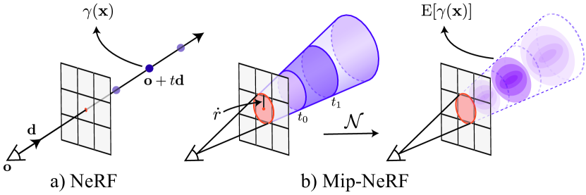
Figure 1: NeRF (a) samples points $\mathbf{x}$ along rays that are traced from the camera center of projection through each pixel, then encodes those points with a positional encoding (PE) $\gamma$ to produce a feature $\gamma(\mathbf{x})$. Mip-NeRF (b) instead reasons about the 3D conical frustum defined by a camera pixel. These conical frustums are then featurized with our integrated positional encoding (IPE), which works by approximating the frustum with a multivariate Gaussian and then computing the (closed form) integral $\operatorname{E}[\gamma(\mathbf{x})]$ over the positional encodings of the coordinates within the Gaussian.

In this paper, we take inspiration from the mipmapping approach used to prevent aliasing in computer graphics rendering pipelines. A mipmap represents a signal (typically an image or a texture map) at a set of different discrete downsampling scales and selects the appropriate scale to use for a ray based on the projection of the pixel footprint onto the geometry intersected by that ray. This strategy is known as pre-filtering, since the computational burden of anti-aliasing is shifted from render time (as in the brute force supersampling solution) to a precomputation phase— the mipmap need only be created once for a given texture, regardless of how many times that texture is rendered.

Our solution, which we call mip-NeRF (multum in parvo NeRF, as in “mipmap”), extends NeRF to simultaneously represent the prefiltered radiance field for a continuous space of scales. The input to mip-NeRF is a 3D Gaussian that represents the region over which the radiance field should be integrated. As illustrated in Figure 1, we can then render a prefiltered pixel by querying mip-NeRF at intervals along a cone, using Gaussians that approximate the conical frustums corresponding to the pixel. To encode a 3D position and its surrounding Gaussian region, we propose a new feature representation: an integrated positional encoding (IPE). This is a generalization of NeRF’s positional encoding (PE) that allows a region of space to be compactly featurized, as opposed to a single point in space.

Mip-NeRF substantially improves upon the accuracy of NeRF, and this benefit is even greater in situations where scene content is observed at different resolutions (i.e. setups where the camera moves closer and farther from the scene). On a challenging multiresolution benchmark we present, mip-NeRF is able to reduce error rates relative to NeRF by $60\%$ on average (see Figure 2 for visualisations). Mip-NeRF’s scale-aware structure also allows us to merge the separate “coarse” and “fine” MLPs used by NeRF for hierarchical sampling [mildenhall2020] into a single MLP. As a consequence, mip-NeRF is slightly faster than NeRF ($\sim 7\%$), and has half as many parameters.

Full Resolution	\begin{overpic}[width=56.3705pt]{figures/aliasing2/nerf_full.png} \put(48.0,2.0){\scriptsize 0.954} \end{overpic}	\begin{overpic}[width=56.3705pt]{figures/aliasing2/mnerf_full.png} \put(48.0,2.0){\scriptsize 0.863} \end{overpic}	\begin{overpic}[width=56.3705pt]{figures/aliasing2/mip_full.png} \put(48.0,2.0){\scriptsize\color[rgb]{0.85,0.0,0.0} 0.962} \end{overpic}	\begin{overpic}[width=56.3705pt]{figures/aliasing2/gt_full.png} \put(48.0,2.0){\scriptsize} \end{overpic}
$\nicefrac{{1}}{{8}}$ Resolution	\begin{overpic}[width=56.3705pt]{figures/aliasing2/nerf_down.png} \put(48.0,2.0){\scriptsize 0.751} \end{overpic}	\begin{overpic}[width=56.3705pt]{figures/aliasing2/mnerf_down.png} \put(48.0,2.0){\scriptsize 0.835} \end{overpic}	\begin{overpic}[width=56.3705pt]{figures/aliasing2/mip_down.png} \put(48.0,2.0){\scriptsize\color[rgb]{0.85,0.0,0.0} 0.976} \end{overpic}	\begin{overpic}[width=56.3705pt]{figures/aliasing2/gt_down.png} \put(48.0,2.0){\scriptsize} \end{overpic}
	(a) NeRF, Single	(b) NeRF, Multi	(c) Mip-NeRF	(d) Ground Truth

Figure 2: (a, top) A NeRF trained on full-resolution images is capable of producing photorealistic renderings at new view locations, but only at the resolution or scale of the training images. (a, bottom) Pulling the camera back and zooming in (or similarly, adjusting the camera intrinsics to reduce image resolution, as is done here) results in renderings that exhibit severe aliasing. (b) Training a NeRF on multi-resolution images ameliorates this issue slightly but results in poor quality renderings across scales: blur at full resolution, and “jaggies” at low resolutions. (c) Mip-NeRF, also trained on multi-resolution images, is capable of producing photorealistic renderings across different scales. SSIMs for each image relative to the ground-truth (d) are inset, with the highest SSIM for both scales shown in red.

2 Related Work

Our work directly extends NeRF [mildenhall2020], a highly influential technique for learning a 3D scene representation from observed images in order to synthesize novel photorealistic views. Here we review the 3D representations used by computer graphics and view synthesis, including recently-introduced continuous neural representations such as NeRF, with a focus on sampling and aliasing.

Anti-aliasing in Rendering    Sampling and aliasing are fundamental issues that have been extensively studied throughout the development of rendering algorithms in computer graphics. Reducing aliasing artifacts (“anti-aliasing”) is typically done via either supersampling or prefiltering. Supersampling-based techniques [whitted80] cast multiple rays per pixel while rendering in order to sample closer to the Nyquist frequency. This is an effective strategy to reduce aliasing, but it is expensive, as runtime generally scales linearly with the supersampling rate. Supersampling is therefore typically used only in offline rendering contexts. Instead of sampling more rays to match the Nyquist frequency, prefiltering-based techniques use lowpass-filtered versions of scene content to decrease the Nyquist frequency required to render the scene without aliasing. Prefiltering techniques [Kaplanyan2016, Neumip, Olano, Lifan2019] are better suited for realtime rendering, because filtered versions of scene content can be precomputed ahead of time, and the correct “scale” can be used at render time depending on the target sampling rate. In the context of rendering, prefiltering can be thought of as tracing a cone instead of a ray through each pixel [amanatides1984ray, igehy1999]: wherever the cone intersects scene content, a precomputed multiscale representation of the scene content (such as a sparse voxel octree [Heitz2012, laine10] or a mipmap [williams83]) is queried at the scale corresponding to the cone’s footprint.

Our work takes inspiration from this line of work in graphics and presents a multiscale scene representation for NeRF. Our strategy differs from multiscale representations used in traditional graphics pipelines in two crucial ways. First, we cannot precompute the multiscale representation because the scene’s geometry is not known ahead of time in our problem setting — we are recovering a model of the scene using computer vision, not rendering a predefined CGI asset. Mip-NeRF therefore must learn a prefiltered representation of the scene during training. Second, our notion of scale is continuous instead of discrete. Instead of representing the scene using multiple copies at a fixed number of scales (like in a mipmap), mip-NeRF learns a single neural scene model that can be queried at arbitrary scales.

Scene Representations for View Synthesis    Various scene representations have been proposed for the task of view synthesis: using observed images of a scene to recover a representation that supports rendering novel photorealistic images of the scene from unobserved camera viewpoints. When images of the scene are captured densely, light field interpolation techniques [davis12, gortler96, levoy96] can be used to render novel views without reconstructing an intermediate representation of the scene. Issues related to sampling and aliasing have been thoroughly studied within this setting [chai00].

Methods that synthesize novel views from sparsely-captured images typically reconstruct explicit representations of the scene’s 3D geometry and appearance. Many classic view synthesis algorithms use mesh-based representations along with either diffuse [waechter2014] or view-dependent [buehler01, debevec96, wood00] textures. Mesh-based representations can be stored efficiently and are naturally compatible with existing graphics rendering pipelines. However, using gradient-based methods to optimize mesh geometry and topology is typically difficult due to discontinuities and local minima. Volumetric representations have therefore become increasingly popular for view synthesis. Early approaches directly color voxel grids using observed images [seitz99], and more recent volumetric approaches use gradient-based learning to train deep networks to predict voxel grid representations of scenes [flynn19, neuralvolumes, mildenhall2019, sitzmann19, srinivasan19, zhou18]. Discrete voxel-based representations are effective for view synthesis, but they do not scale well to scenes at higher resolutions.

A recent trend within computer vision and graphics research is to replace these discrete representations with coordinate-based neural representations, which represent 3D scenes as continuous functions parameterized by MLPs that map from a 3D coordinate to properties of the scene at that location. Some recent methods use coordinate-based neural representations to model scenes as implicit surfaces [niemeyer2020dvr, yariv2020multiview], but the majority of recent view synthesis methods are based on the volumetric NeRF representation [mildenhall2020]. NeRF has inspired many subsequent works that extend its continuous neural volumetric representation for generative modeling [chan2020pi, schwarz2020graf], dynamic scenes [li2021, ost2020neural], non-rigidly deforming objects [gafni2020dynamic, park2020deformable], phototourism settings with changing illumination and occluders [martinbrualla2020nerfw, tancik2020meta], and reflectance modeling for relighting [bi2020, boss2020nerd, nerv2021].

Relatively little attention has been paid to the issues of sampling and aliasing within the context of view synthesis using coordinate-based neural representations. Discrete representations used for view synthesis, such as polygon meshes and voxel grids, can be efficiently rendered without aliasing using traditional multiscale prefiltering approaches such as mipmaps and octrees. However, coordinate-based neural representations for view synthesis can currently only be anti-aliased using supersampling, which exacerbates their already slow rendering procedure. Recent work by Takikawa et al. [takikawa21] proposes a multiscale representation based on sparse voxel octrees for continuous neural representations of implicit surfaces, but their approach requires that the scene geometry be known a priori, as opposed to our view synthesis setting where the only inputs are observed images. Mip-NeRF addresses this open problem, enabling the efficient rendering of anti-aliased images during both training and testing as well as the use of multiscale images during training.

2.1 Preliminaries: NeRF

NeRF uses the weights of a multilayer perceptron (MLP) to represent a scene as a continuous volumetric field of particles that block and emit light. NeRF renders each pixel of a camera as follows: A ray $\mathbf{r}(t)=\mathbf{o}+t\mathbf{d}$ is emitted from the camera’s center of projection $\mathbf{o}$ along the direction $\mathbf{d}$ such that it passes through the pixel. A sampling strategy (discussed later) is used to determine a vector of sorted distances $\mathbf{t}$ between the camera’s predefined near and far planes $t_{n}$ and $t_{f}$. For each distance $t_{k}\in\mathbf{t}$, we compute its corresponding 3D position along the ray $\mathbf{x}=\mathbf{r}(t_{k})$, then transform each position using a positional encoding:

$$\gamma(\mathbf{x})\!=\!\Big{[}\sin(\mathbf{x}),\cos(\mathbf{x}),\ldots,\sin\!\big{(}2^{L-1}\mathbf{x}\big{)},\cos\!\big{(}2^{L-1}\mathbf{x}\big{)}\Big{]}^{\operatorname{T}}\,.$$ (1)

This is simply the concatenation of the sines and cosines of each dimension of the 3D position $\mathbf{x}$ scaled by powers of 2 from $1$ to $2^{L-1}$, where $L$ is a hyperparameter. The fidelity of NeRF depends critically on the use of positional encoding, as it allows the MLP parameterizing the scene to behave as an interpolation function, where $L$ determines the bandwidth of the interpolation kernel (see Tancik et al. [tancik2020fourfeat] for details). The positional encoding of each ray position $\gamma(\mathbf{r}(t_{k}))$ is provided as input to an MLP parameterized by weights $\Theta$, which outputs a density $\tau$ and an RGB color $\mathbf{c}$:

$$\forall t_{k}\in\mathbf{t},\quad[\tau_{k},\,\mathbf{c}_{k}]=\operatorname{MLP}\mathopen{}\mathclose{{}\left(\gamma\mathopen{}\mathclose{{}\left(\mathbf{r}(t_{k})}\right);\,\Theta}\right)\,.$$ (2)

The MLP also takes the view direction as input, which is omitted from notation for simplicity. These estimated densities and colors are used to approximate the volume rendering integral using numerical quadrature, as per Max [max1995optical]:

$$\mathbf{C}(\mathbf{r};\Theta,\mathbf{t})=\sum_{k}T_{k}\mathopen{}\mathclose{{}\left(1-\exp(-\tau_{k}(t_{k+1}-t_{k}))}\right)\mathbf{c}_{k}\,,$$

$$\textrm{with}\quad T_{k}=\exp\bigg{(}\!-\!\sum_{k^{\prime}<k}\tau_{k^{\prime}}\mathopen{}\mathclose{{}\left(t_{k^{\prime}+1}-t_{k^{\prime}}}\right)\!\bigg{)}\,,$$ (3)

where $\mathbf{C}(\mathbf{r};\Theta,\mathbf{t})$ is the final predicted color of the pixel.

With this procedure for rendering a NeRF parameterized by $\Theta$, training a NeRF is straightforward: using a set of observed images with known camera poses, we minimize the sum of squared differences between all input pixel values and all predicted pixel values using gradient descent. To improve sample efficiency, NeRF trains two separate MLPs, one “coarse” and one “fine”, with parameters $\Theta^{c}$ and $\Theta^{f}$:

$$\underset{\Theta^{c},\Theta^{f}}{\operatorname{min}}\,\sum_{\mathbf{r}\in\mathcal{R}}\Big{(} \big{\|}\mathbf{C}^{*}(\mathbf{r})-\mathbf{C}(\mathbf{r};\Theta^{c},\mathbf{t}^{c})\big{\|}_{2}^{2}$$ (4)

$$+ \big{\|}\mathbf{C}^{*}(\mathbf{r})-\mathbf{C}(\mathbf{r};\Theta^{f},\operatorname{sort}(\mathbf{t}^{c}\cup\mathbf{t}^{f}))\big{\|}_{2}^{2}\Big{)}\,,$$

where $\mathbf{C}^{*}(\mathbf{r})$ is the observed pixel color taken from the input image, and $\mathcal{R}$ is the set of all pixels/rays across all images. Mildenhall et al. construct $\mathbf{t}^{c}$ by sampling $64$ evenly-spaced random $t$ values with stratified sampling. The compositing weights $w_{k}=T_{k}\,\mathopen{}\mathclose{{}\left(1-\exp(-\tau_{k}(t_{k+1}-t_{k}))}\right)$ produced by the “coarse” model are then taken as a piecewise constant PDF describing the distribution of visible scene content, and $128$ new $t$ values are drawn from that PDF using inverse transform sampling to produce $\mathbf{t}^{f}$. The union of these $192$ $t$ values are then sorted and passed to the “fine” MLP to produce a final predicted pixel color.

3 Method

As discussed, NeRF’s point-sampling makes it vulnerable to issues related to sampling and aliasing: Though a pixel’s color is the integration of all incoming radiance within the pixel’s frustum, NeRF casts a single infinitesimally narrow ray per pixel, resulting in aliasing. Mip-NeRF ameliorates this issue by casting a cone from each pixel. Instead of performing point-sampling along each ray, we divide the cone being cast into a series of conical frustums (cones cut perpendicular to their axis). And instead of constructing positional encoding (PE) features from an infinitesimally small point in space, we construct an integrated positional encoding (IPE) representation of the volume covered by each conical frustum. These changes allow the MLP to reason about the size and shape of each conical frustum, instead of just its centroid. The ambiguity resulting from NeRF’s insensitivity to scale and mip-NeRF’s solution to this problem are visualized in Figure 3. This use of conical frustums and IPE features also allows us to reduce NeRF’s two separate “coarse” and “fine” MLPs into a single multiscale MLP, which increases training and evaluation speed and reduces model size by $50\%$.

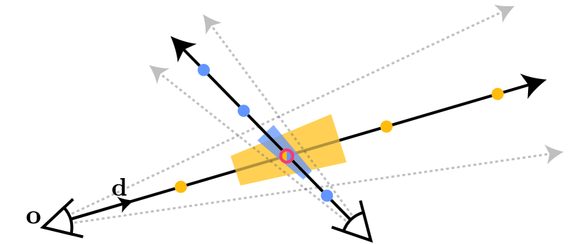
Figure 3: NeRF works by extracting point-sampled positional encoding features (shown here as dots) along each pixel’s ray. Those point-sampled features ignore the shape and size of the volume viewed by each ray, so two different cameras imaging the same position at different scales may produce the same ambiguous point-sampled feature, thereby significantly degrading NeRF’s performance. In contrast, Mip-NeRF casts cones instead of rays and explicitly models the volume of each sampled conical frustum (shown here as trapezoids), thus resolving this ambiguity.

3.1 Cone Tracing and Positional Encoding

Here we describe mip-NeRF’s rendering and featurization procedure, in which we cast a cone and featurize conical frustums along that cone. As in NeRF, images in mip-NeRF are rendered one pixel at a time, so we can describe our procedure in terms of an individual pixel of interest being rendered. For that pixel, we cast a cone from the camera’s center of projection $\mathbf{o}$ along the direction $\mathbf{d}$ that passes through the pixel’s center. The apex of that cone lies at $\mathbf{o}$, and the radius of the cone at the image plane $\mathbf{o}+\mathbf{d}$ is parameterized as $\dot{r}$. We set $\dot{r}$ to the width of the pixel in world coordinates scaled by $\nicefrac{{2}}{{\sqrt{12}}}$, which yields a cone whose section on the image plane has a variance in $x$ and $y$ that matches the variance of the pixel’s footprint. The set of positions $\mathbf{x}$ that lie within a conical frustum between two $t$ values $[t_{0},t_{1}]$ (visualized in Figure 1) is:

$$\operatorname{F}(\mathbf{x},\mathbf{o},\mathbf{d},\dot{r},t_{0},t_{1})=\mathbbm{1}\Bigg{\{}\mathopen{}\mathclose{{}\left(t_{0}<\frac{\mathbf{d}^{\operatorname{T}}(\mathbf{x}-\mathbf{o})}{\mathopen{}\mathclose{{}\left\lVert\mathbf{d}}\right\rVert^{2}_{2}}<t_{1}}\right)$$

$$\land\,\mathopen{}\mathclose{{}\left(\frac{\mathbf{d}^{\operatorname{T}}(\mathbf{x}-\mathbf{o})}{\mathopen{}\mathclose{{}\left\lVert\mathbf{d}}\right\rVert_{2}\mathopen{}\mathclose{{}\left\lVert\mathbf{x}-\mathbf{o}}\right\rVert_{2}}>\frac{1}{\sqrt{1+(\dot{r}/\mathopen{}\mathclose{{}\left\lVert\mathbf{d}}\right\rVert_{2})^{2}}}}\right)\Bigg{\}}\,,$$ (5)

where $\mathbbm{1}\{\cdot\}$ is an indicator function: $\operatorname{F}(\mathbf{x},\cdot)=1$ iff $\mathbf{x}$ is within the conical frustum defined by $(\mathbf{o},\mathbf{d},\dot{r},t_{0},t_{1})$.

We must now construct a featurized representation of the volume inside this conical frustum. Ideally, this featurized representation should be of a similar form to the positional encoding features used in NeRF, as Mildenhall et al. show that this feature representation is critical to NeRF’s success [mildenhall2020]. There are many viable approaches for this (see the supplement for further discussion) but the simplest and most effective solution we found was to simply compute the expected positional encoding of all coordinates that lie within the conical frustum:

$$\gamma^{*}(\mathbf{o},\mathbf{d},\dot{r},t_{0},t_{1})=\frac{\int\gamma(\mathbf{x})\operatorname{F}(\mathbf{x},\mathbf{o},\mathbf{d},\dot{r},t_{0},t_{1})\,d\mathbf{x}}{\int\operatorname{F}(\mathbf{x},\mathbf{o},\mathbf{d},\dot{r},t_{0},t_{1})\,d\mathbf{x}}\,.$$ (6)

However, it is unclear how such a feature could be computed efficiently, as the integral in the numerator has no closed form solution. We therefore approximate the conical frustum with a multivariate Gaussian which allows for an efficient approximation to the desired feature, which we will call an “integrated positional encoding” (IPE).

To approximate a conical frustum with a multivariate Gaussian, we must compute the mean and covariance of $\operatorname{F}(\mathbf{x},\cdot)$. Because each conical frustum is assumed to be circular, and because conical frustums are symmetric around the axis of the cone, such a Gaussian is fully characterized by three values (in addition to $\mathbf{o}$ and $\mathbf{d}$): the mean distance along the ray $\mu_{t}$, the variance along the ray $\sigma_{t}^{2}$, and the variance perpendicular to the ray $\sigma_{r}^{2}$:

$$\mu_{t}=t_{\mu}+\frac{2t_{\mu}t_{\delta}^{2}}{3t_{\mu}^{2}+t_{\delta}^{2}}\,,\quad\,\,\sigma_{t}^{2}=\frac{t_{\delta}^{2}}{3}-\frac{4t_{\delta}^{4}(12t_{\mu}^{2}-t_{\delta}^{2})}{15(3t_{\mu}^{2}+t_{\delta}^{2})^{2}}\,,$$

$$\sigma_{r}^{2}=\dot{r}^{2}\mathopen{}\mathclose{{}\left(\frac{t_{\mu}^{2}}{4}+\frac{5t_{\delta}^{2}}{12}-\frac{4t_{\delta}^{4}}{15(3t_{\mu}^{2}+t_{\delta}^{2})}}\right)\,.$$ (7)

These quantities are parameterized with respect to a midpoint $t_{\mu}=(t_{0}+t_{1})/2$ and a half-width $t_{\delta}=(t_{1}-t_{0})/2$, which is critical for numerical stability. Please refer to the supplement for a detailed derivation. We can transform this Gaussian from the coordinate frame of the conical frustum into world coordinates as follows:

$$\boldsymbol{\mu}=\mathbf{o}+\mu_{t}\mathbf{d}\,,\quad\,\,\boldsymbol{\Sigma}=\sigma_{t}^{2}\mathopen{}\mathclose{{}\left(\mathbf{d}\mathbf{d}^{\operatorname{T}}}\right)+\sigma_{r}^{2}\mathopen{}\mathclose{{}\left(\mathbf{I}-\frac{\mathbf{d}\mathbf{d}^{\operatorname{T}}}{\mathopen{}\mathclose{{}\left\lVert\mathbf{d}}\right\rVert_{2}^{2}}}\right)\,,$$ (8)

giving us our final multivariate Gaussian.

Next, we derive the IPE, which is the expectation of a positionally-encoded coordinate distributed according to the aforementioned Gaussian. To accomplish this, it is helpful to first rewrite the PE in Equation 1 as a Fourier feature [Rahimi2007, tancik2020fourfeat]:

$$\mathbf{P}\!=\!\!\begin{bmatrix}1\!\!&\!\!0\!\!&\!\!0\!\!&\!\!2\!\!&\!\!0\!\!&\!\!0\!\!&\!\!\!\!\!\!&\!\!\!\!2^{L-1}\!\!\!\!&\!\!\!\!0\!\!\!\!&\!\!\!\!0\!\!\\ 0\!\!&\!\!1\!\!&\!\!0\!\!&\!\!0\!\!&\!\!2\!\!&\!\!0\!\!&\!\!\!\cdots\!\!\!&\!\!\!\!0\!\!\!\!&\!\!\!\!2^{L-1}\!\!\!\!&\!\!\!\!0\!\!\!\\ 0\!\!&\!\!0\!\!&\!\!1\!\!&\!\!0\!\!&\!\!0\!\!&\!\!2\!\!&\!\!\!\!\!\!&\!\!\!0\!\!\!\!&\!\!\!\!0\!\!\!&\!\!\!\!2^{L-1}\!\!\\ \end{bmatrix}^{\operatorname{T}}\!\!\!\!,\,\,\,\gamma(\mathbf{x})\!=\!\!\begin{bmatrix}\sin(\mathbf{P}\mathbf{x})\\ \cos(\mathbf{P}\mathbf{x})\end{bmatrix}\,.$$ (9)

This reparameterization allows us to derive a closed form for IPE. Using the fact that the covariance of a linear transformation of a variable is a linear transformation of the variable’s covariance ($\operatorname{Cov}[\mathbf{A}\mathbf{x},\mathbf{B}\mathbf{y}]=\mathbf{A}\operatorname{Cov}[\mathbf{x},\mathbf{y}]\mathbf{B}^{\operatorname{T}}$) we can identify the mean and covariance of our conical frustum Gaussian after it has been lifted into the PE basis $\mathbf{P}$:

$$\boldsymbol{\mu}_{\gamma}=\mathbf{P}\boldsymbol{\mu}\,,\quad\,\,\boldsymbol{\Sigma}_{\gamma}=\mathbf{P}\boldsymbol{\Sigma}\mathbf{P}^{\operatorname{T}}\,.$$ (10)

The final step in producing an IPE feature is computing the expectation over this lifted multivariate Gaussian, modulated by the sine and the cosine of position. These expectations have simple closed-form expressions:

$$\operatorname{E}_{x\sim\mathcal{N}(\mu,\sigma^{2})}\mathopen{}\mathclose{{}\left[\sin(x)}\right] =\sin(\mu)\exp\mathopen{}\mathclose{{}\left(-(\nicefrac{{1}}{{2}})\sigma^{2}}\right)\,,$$ (11)

$$\operatorname{E}_{x\sim\mathcal{N}(\mu,\sigma^{2})}\mathopen{}\mathclose{{}\left[\cos(x)}\right] =\cos(\mu)\exp\mathopen{}\mathclose{{}\left(-(\nicefrac{{1}}{{2}})\sigma^{2}}\right)\,.$$ (12)

We see that this expected sine or cosine is simply the sine or cosine of the mean attenuated by a Gaussian function of the variance. With this we can compute our final IPE feature as the expected sines and cosines of the mean and the diagonal of the covariance matrix:

$$\gamma(\boldsymbol{\mu},\boldsymbol{\Sigma}) =\operatorname{E}_{\mathbf{x}\sim\mathcal{N}(\boldsymbol{\mu}_{\gamma},\boldsymbol{\Sigma}_{\gamma})}\mathopen{}\mathclose{{}\left[\gamma(\mathbf{x})}\right]$$ (13)

$$=\begin{bmatrix}\sin(\boldsymbol{\mu}_{\gamma})\circ\exp\mathopen{}\mathclose{{}\left(-(\nicefrac{{1}}{{2}})\operatorname{diag}\mathopen{}\mathclose{{}\left(\boldsymbol{\Sigma}_{\gamma}}\right)}\right)\\ \cos(\boldsymbol{\mu}_{\gamma})\circ\exp\mathopen{}\mathclose{{}\left(-(\nicefrac{{1}}{{2}})\operatorname{diag}\mathopen{}\mathclose{{}\left(\boldsymbol{\Sigma}_{\gamma}}\right)}\right)\end{bmatrix}\,,$$ (14)

where $\circ$ denotes element-wise multiplication. Because positional encoding encodes each dimension independently, this expected encoding relies on only the marginal distribution of $\gamma(\mathbf{x})$, and only the diagonal of the covariance matrix (a vector of per-dimension variances) is needed. Because $\boldsymbol{\Sigma}_{\gamma}$ is prohibitively expensive to compute due its relatively large size, we directly compute the diagonal of $\boldsymbol{\Sigma}_{\gamma}$:

$$\small\operatorname{diag}(\boldsymbol{\Sigma}_{\gamma})\!=\!\mathopen{}\mathclose{{}\left[\operatorname{diag}(\boldsymbol{\Sigma}),4\operatorname{diag}(\boldsymbol{\Sigma}),\ldots,4^{L-1}\operatorname{diag}(\boldsymbol{\Sigma})}\right]^{\operatorname{T}}$$ (15)

This vector depends on just the diagonal of the 3D position’s covariance $\boldsymbol{\Sigma}$, which can be computed as:

$$\operatorname{diag}(\boldsymbol{\Sigma})=\sigma_{t}^{2}\mathopen{}\mathclose{{}\left(\mathbf{d}\circ\mathbf{d}}\right)+\sigma_{r}^{2}\mathopen{}\mathclose{{}\left(\mathbf{1}-\frac{\mathbf{d}\circ\mathbf{d}}{\mathopen{}\mathclose{{}\left\lVert\mathbf{d}}\right\rVert_{2}^{2}}}\right)\,.$$ (16)

If these diagonals are computed directly, IPE features are roughly as expensive as PE features to construct.

Figure 4 visualizes the difference between IPE and conventional PE features in a toy 1D domain. IPE features behave intuitively: If a particular frequency in the positional encoding has a period that is larger than the width of the interval being used to construct the IPE feature, then the encoding at that frequency is unaffected. But if the period is smaller than the interval (in which case the PE over that interval will oscillate repeatedly), then the encoding at that frequency is scaled down towards zero. In short, IPE preserves frequencies that are constant over an interval and softly “removes” frequencies that vary over an interval, while PE preserves all frequencies up to some manually-tuned hyperparameter $L$. By scaling each sine and cosine in this way, IPE features are effectively anti-aliased positional encoding features that smoothly encode the size and shape of a volume of space. IPE also effectively removes $L$ as a hyperparameter: it can simply be set to an extremely large value and then never tuned (see supplement).

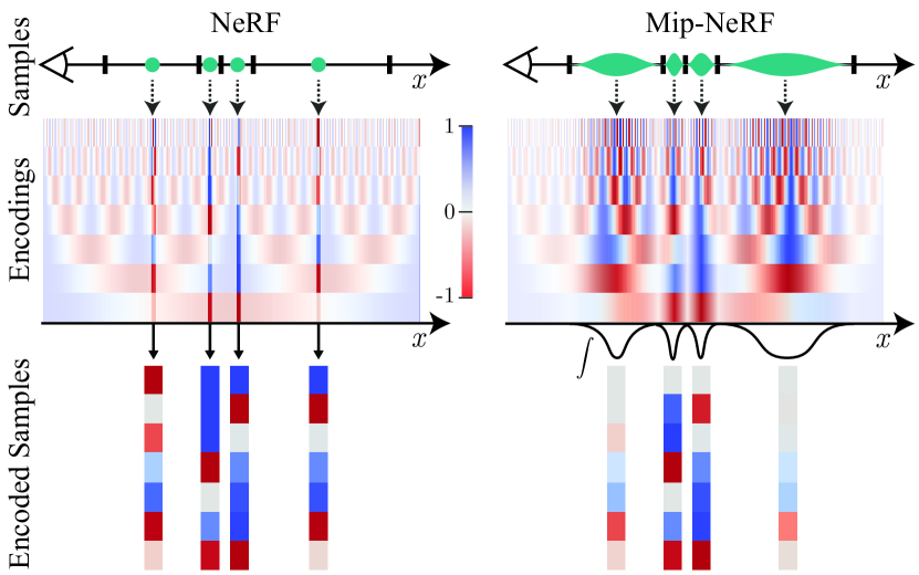
Figure 4: Toy 1D visualizations of the positional encoding (PE) used by NeRF (left) and our integrated positional encoding (IPE) (right). Because NeRF samples points along each ray and encodes all frequencies equally, the high-frequency PE features are aliased, which results in rendering artifacts. By integrating PE features over each interval, the high frequency dimensions of IPE features shrink towards zero when the period of the frequency is small compared to the size of the interval being integrated, resulting in anti-aliased features that implicitly encode the size (and in higher dimensions, the shape) of the interval.

3.2 Architecture

Aside from cone-tracing and IPE features, mip-NeRF behaves similarly to NeRF, as described in Section 2.1. For each pixel being rendered, instead of a ray as in NeRF, a cone is cast. Instead of sampling $n$ values for $t_{k}$ along the ray, we sample $n+1$ values for $t_{k}$, computing IPE features for the interval spanning each adjacent pair of sampled $t_{k}$ values as previously described. These IPE features are passed as input into an MLP to produce a density $\tau_{k}$ and a color $\mathbf{c}_{k}$, as in Equation 2. Rendering in mip-NeRF follows Equation 3.

Recall that NeRF uses a hierarchical sampling procedure with two distinct MLPs, one “coarse” and one “fine” (see Equation 4). This was necessary in NeRF because its PE features meant that its MLPs were only able to learn a model of the scene for one single scale. But our cone casting and IPE features allow us to explicitly encode scale into our input features and thereby enable an MLP to learn a multiscale representation of the scene. Mip-NeRF therefore uses a single MLP with parameters $\Theta$, which we repeatedly query in a hierarchical sampling strategy. This has multiple benefits: model size is cut in half, renderings are more accurate, sampling is more efficient, and the overall algorithm becomes simpler. Our optimization problem is:

$$\underset{\Theta}{\operatorname{min}}\,\sum_{\mathbf{r}\in\mathcal{R}}\Big{(}\lambda\big{\|}\mathbf{C}^{*}(\mathbf{r})-\mathbf{C}(\mathbf{r};\Theta,\mathbf{t}^{c})\big{\|}_{2}^{2}+\big{\|}\mathbf{C}^{*}(\mathbf{r})-\mathbf{C}(\mathbf{r};\Theta,\mathbf{t}^{f})\big{\|}_{2}^{2}\Big{)}$$ (17)

Because we have a single MLP, the “coarse” loss must be balanced against the “fine” loss, which is accomplished using a hyperparameter $\lambda$ (we set $\lambda=0.1$ in all experiments). As in Mildenhall et al. [mildenhall2020], our coarse samples $\mathbf{t}^{c}$ are produced with stratified sampling, and our fine samples $\mathbf{t}^{f}$ are sampled from the resulting alpha compositing weights $\mathbf{w}$ using inverse transform sampling. Unlike NeRF, in which the fine MLP is given the sorted union of $64$ coarse samples and $128$ fine samples, in mip-NeRF we simply sample $128$ samples for the coarse model and $128$ samples from the fine model (yielding the same number of total MLP evaluations as in NeRF, for fair comparison). Before sampling $\mathbf{t}^{f}$, we modify the weights $\mathbf{w}$ slightly:

$$w^{\prime}_{k}=\frac{1}{2}\mathopen{}\mathclose{{}\left(\max(w_{k-1},w_{k})+\max(w_{k},w_{k+1})}\right)+\alpha\,.$$ (18)

We filter $\mathbf{w}$ with a 2-tap max filter followed by a 2-tap blur filter (a “blurpool” [zhang2019making]), which produces a wide and smooth upper envelope on $\mathbf{w}$. A hyperparameter $\alpha$ is added to that envelope before it is re-normalized to sum to $1$, which ensures that some samples are drawn even in empty regions of space (we set $\alpha=0.01$ in all experiments).

Mip-NeRF is implemented on top of JaxNeRF [jaxnerf2020github], a JAX [jax2018github] reimplementation of NeRF that achieves better accuracy and trains faster than the original TensorFlow implementation. We follow NeRF’s training procedure: 1 million iterations of Adam [adam] with a batch size of $4096$ and a learning rate that is annealed logarithmically from $5\cdot 10^{-4}$ to $5\cdot 10^{-6}$. See the supplement for additional details and some additional differences between JaxNeRF and mip-NeRF that do not affect performance significantly and are incidental to our primary contributions: cone-tracing, IPE, and the use of a single multiscale MLP.

4 Results

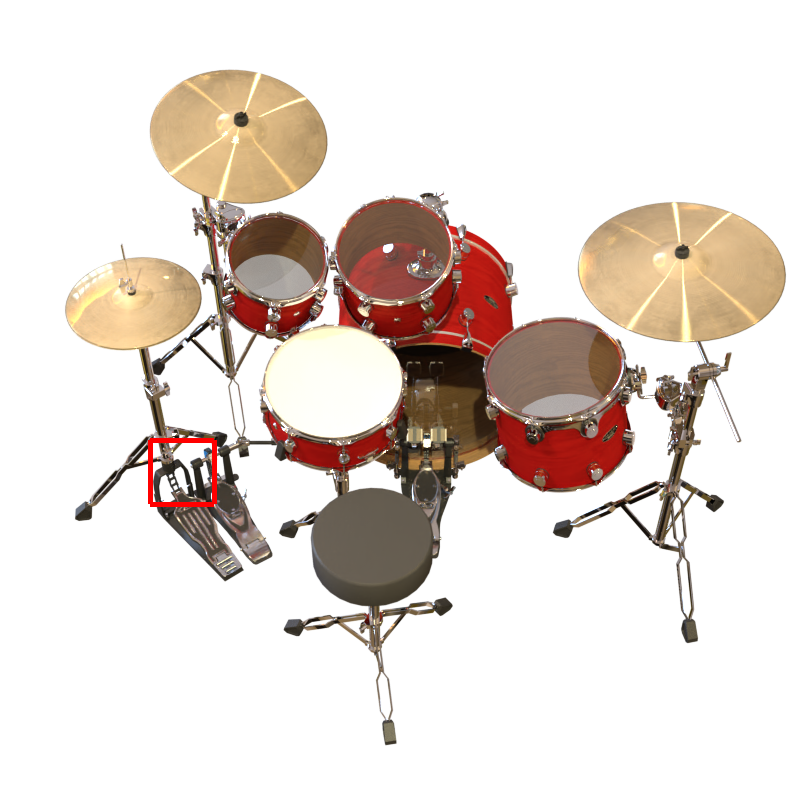
	\begin{overpic}[width=93.95122pt]{figures/multiblender_pyrs/gt_drums_0_440_150_64.png} \put(67.0,2.0){\tiny\lx@texthl@color{$$}} \put(84.0,29.0){\tiny\lx@texthl@color{$$}} \put(84.0,18.0){\tiny\lx@texthl@color{$$}} \put(76.0,10.0){\tiny\lx@texthl@color{$$}} \end{overpic}	\begin{overpic}[width=93.95122pt]{figures/multiblender_pyrs/jaxnerf_multiblender_drums_0_440_150_64.png} \put(67.0,2.0){\tiny\lx@texthl@color{$0.709$}} \put(84.0,29.0){\tiny\lx@texthl@color{$0.910$}} \put(84.0,18.0){\tiny\lx@texthl@color{$0.931$}} \put(76.0,10.0){\tiny\lx@texthl@color{$0.663$}} \end{overpic}	\begin{overpic}[width=93.95122pt]{figures/multiblender_pyrs/jaxnerf_multiblender_extras_drums_0_440_150_64.png} \put(67.0,2.0){\tiny\lx@texthl@color{$0.863$}} \put(84.0,29.0){\tiny\lx@texthl@color{$0.959$}} \put(84.0,18.0){\tiny\lx@texthl@color{$0.971$}} \put(76.0,10.0){\tiny\lx@texthl@color{$0.881$}} \end{overpic}	\begin{overpic}[width=93.95122pt]{figures/multiblender_pyrs/prenerf_multiblender_drums_0_440_150_64.png} \put(67.0,2.0){\tiny\lx@texthl@color{$\color[rgb]{0.85,0.0,0.0}0.940$}} \put(84.0,29.0){\tiny\lx@texthl@color{$\color[rgb]{0.85,0.0,0.0}0.979$}} \put(84.0,18.0){\tiny\lx@texthl@color{$\color[rgb]{0.85,0.0,0.0}0.989$}} \put(76.0,10.0){\tiny\lx@texthl@color{$\color[rgb]{0.85,0.0,0.0}0.978$}} \end{overpic}
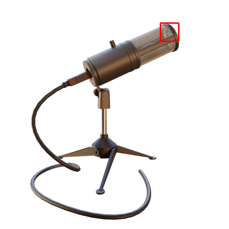
	\begin{overpic}[width=93.95122pt]{figures/multiblender_pyrs/gt_mic_120_80_560_64.png} \put(67.0,2.0){\tiny\lx@texthl@color{$$}} \put(84.0,29.0){\tiny\lx@texthl@color{$$}} \put(84.0,18.0){\tiny\lx@texthl@color{$$}} \put(76.0,10.0){\tiny\lx@texthl@color{$$}} \end{overpic}	\begin{overpic}[width=93.95122pt]{figures/multiblender_pyrs/jaxnerf_multiblender_mic_120_80_560_64.png} \put(67.0,2.0){\tiny\lx@texthl@color{$0.448$}} \put(84.0,29.0){\tiny\lx@texthl@color{$0.562$}} \put(84.0,18.0){\tiny\lx@texthl@color{$0.696$}} \put(76.0,10.0){\tiny\lx@texthl@color{$0.906$}} \end{overpic}	\begin{overpic}[width=93.95122pt]{figures/multiblender_pyrs/jaxnerf_multiblender_extras_mic_120_80_560_64.png} \put(67.0,2.0){\tiny\lx@texthl@color{$0.525$}} \put(84.0,29.0){\tiny\lx@texthl@color{$0.633$}} \put(84.0,18.0){\tiny\lx@texthl@color{$0.794$}} \put(76.0,10.0){\tiny\lx@texthl@color{$0.918$}} \end{overpic}	\begin{overpic}[width=93.95122pt]{figures/multiblender_pyrs/prenerf_multiblender_mic_120_80_560_64.png} \put(67.0,2.0){\tiny\lx@texthl@color{$\color[rgb]{0.85,0.0,0.0}0.785$}} \put(84.0,29.0){\tiny\lx@texthl@color{$\color[rgb]{0.85,0.0,0.0}0.837$}} \put(84.0,18.0){\tiny\lx@texthl@color{$\color[rgb]{0.85,0.0,0.0}0.861$}} \put(76.0,10.0){\tiny\lx@texthl@color{$\color[rgb]{0.85,0.0,0.0}0.975$}} \end{overpic}
Ground-Truth		NeRF	NeRF + Area, Center, Misc	Mip-NeRF

Figure 5: Visualizations of the output of mip-NeRF compared to the ground truth, NeRF, and an improved version of NeRF on test set images from two scenes in our multiscale Blender dataset. We visualize a cropped region of both scenes at 4 different scales, displayed as an image pyramid with the SSIM for each scale shown to its lower right and with the highest SSIM at each scale highlighted in red. Mip-NeRF outperforms NeRF and its improved version by a significant margin, both visually and quantitatively. See the supplement for more such visualizations.

	PSNR $\uparrow$				SSIM $\uparrow$				LPIPS $\downarrow$
	Full Res.	$\nicefrac{{1}}{{2}}$ Res.	$\nicefrac{{1}}{{4}}$ Res.	$\nicefrac{{1}}{{8}}$ Res.	Full Res.	$\nicefrac{{1}}{{2}}$ Res.	$\nicefrac{{1}}{{4}}$ Res.	$\nicefrac{{1}}{{8}}$ Res.	Full Res.	$\nicefrac{{1}}{{2}}$ Res.	$\nicefrac{{1}}{{4}}$ Res.	$\nicefrac{{1}}{{8}}$ Res	Avg. $\downarrow$	Time (hours)	# Params
NeRF (Jax Impl.) [jaxnerf2020github, mildenhall2020]	31.196	30.647	26.252	22.533	0.9498	0.9560	0.9299	0.8709	0.0546	0.0342	0.0428	0.0750	0.0288	3.05 $\pm$ 0.04	1,191K
NeRF + Area Loss	27.224	29.578	29.445	25.039	0.9113	0.9394	0.9524	0.9176	0.1041	0.0677	0.0406	0.0469	0.0305	3.03 $\pm$ 0.03	1,191K
NeRF + Area, Centered Pixels	29.893	32.118	33.399	29.463	0.9376	0.9590	0.9728	0.9620	0.0747	0.0405	0.0245	0.0398	0.0191	3.02 $\pm$ 0.05	1,191K
NeRF + Area, Center, Misc.	29.900	32.127	33.404	29.470	0.9378	0.9592	0.9730	0.9622	0.0743	0.0402	0.0243	0.0394	0.0190	2.94 $\pm$ 0.02	1,191K
Mip-NeRF	32.629	34.336	35.471	35.602	0.9579	0.9703	0.9786	0.9833	0.0469	0.0260	0.0168	0.0120	0.0114	2.84 $\pm$ 0.01	612K
Mip-NeRF w/o Misc.	32.610	34.333	35.497	35.638	0.9577	0.9703	0.9787	0.9834	0.0470	0.0259	0.0167	0.0120	0.0114	2.82 $\pm$ 0.03	612K
Mip-NeRF w/o Single MLP	32.401	34.131	35.462	35.967	0.9566	0.9693	0.9780	0.9834	0.0479	0.0268	0.0169	0.0116	0.0115	3.40 $\pm$ 0.01	1,191K
Mip-NeRF w/o Area Loss	33.059	34.280	33.866	30.714	0.9605	0.9704	0.9747	0.9679	0.0427	0.0256	0.0213	0.0308	0.0139	2.82 $\pm$ 0.01	612K
Mip-NeRF w/o IPE	29.876	32.160	33.679	29.647	0.9384	0.9602	0.9742	0.9633	0.0742	0.0393	0.0226	0.0378	0.0186	2.79 $\pm$ 0.01	612K

Table 1: A quantitative comparison of mip-NeRF and its ablations against NeRF and several NeRF variants on the test set of our multiscale Blender dataset. See the text for details.

We evaluate mip-NeRF on the Blender dataset presented in the original NeRF paper [mildenhall2020] and also on a simple multiscale variant of that dataset designed to better probe accuracy on multi-resolution scenes and to highlight NeRF’s critical vulnerability on such tasks. We report the three error metrics used by NeRF: PSNR, SSIM [wang2004image], and LPIPS [zhang2018unreasonable]. To enable easier comparison, we also present an “average” error metric that summarizes all three metrics: the geometric mean of $\mathrm{MSE}=10^{-\mathrm{PSNR}/10}$, $\sqrt{1-\mathrm{SSIM}}$ (as per [brunet2011mathematical]), and $\mathrm{LPIPS}$. We additionally report runtimes (median and median absolute deviation of wall time) as well as the number of network parameters for each variant of NeRF and mip-NeRF. All JaxNeRF and mip-NeRF experiments are trained on a TPU v2 with 32 cores [jouppi2017datacenter].

We constructed our multiscale Blender benchmark because the original Blender dataset used by NeRF has a subtle but critical weakness: all cameras have the same focal length and resolution and are placed at the same distance from the object. As a result, this Blender task is significantly easier than most real-world datasets, where cameras may be more close or more distant from the subject or may zoom in and out. The limitation of this dataset is complemented by the limitations of NeRF: despite NeRF’s tendency to produce aliased renderings, it is able to produce excellent results on the Blender dataset because that dataset systematically avoids this failure mode.

Multiscale Blender Dataset    Our multiscale Blender dataset is a straightforward modification to NeRF’s Blender dataset, designed to probe aliasing and scale-space reasoning. This dataset was constructed by taking each image in the Blender dataset, box downsampling it a factor of $2$, $4$, and $8$ (and modifying the camera intrinsics accordingly), and combining the original images and the three downsampled images into one single dataset. Due to the nature of projective geometry, this is similar to re-rendering the original dataset where the distance to the camera has been increased by scale factors of $2$, $4$, and $8$. When training mip-NeRF on this dataset, we scale the loss of each pixel by the area of that pixel’s footprint in the original image (the loss for pixels from the $\nicefrac{{1}}{{4}}$ images is scaled by $16$, etc) so that the few low-resolution pixels have comparable influence to the many high-resolution pixels. The average error metric for this task uses the arithmetic mean of each error metric across all four scales.

The performance of mip-NeRF for this multiscale dataset can be seen in Table 4. Because NeRF is the state of the art on the Blender dataset (as will be shown in Table 4), we evaluate against only NeRF and several improved versions of NeRF: “Area Loss” adds the aforementioned scaling of the loss function by pixel area used by mip-NeRF, “Centered Pixels” adds a half-pixel offset added to each ray’s direction such that rays pass through the center of each pixel (as opposed to the corner of each pixel as was done in Mildenhall et al.) and “Misc” adds some small changes that slightly improve the stability of training (see supplement). We also evaluate against several ablations of mip-NeRF: “w/o Misc” removes those small changes, “w/o Single MLP” uses NeRF’s two-MLP training scheme from Equation 4, “w/o Area Loss” removes the loss scaling by pixel area, and “w/o IPE” uses PE instead of IPE, which causes mip-NeRF to use NeRF’s ray-casting (with centered pixels) instead of our cone-casting.

Mip-NeRF reduces average error by $60\%$ on this task and outperforms NeRF by a large margin on all metrics and all scales. “Centering” pixels improves NeRF’s performance substantially, but not enough to approach mip-NeRF. Removing IPE features causes mip-NeRF’s performance to degrade to the performance of “Centered” NeRF, thereby demonstrating that cone-casting and IPE features are the primary factors driving performance (though the area loss contributes substantially). The “Single MLP” mip-NeRF ablation performs well but has twice as many parameters and is nearly $20\%$ slower than mip-NeRF (likely due to this ablation’s need to sort $t$ values and poor hardware throughput due to its changing tensor sizes across its “coarse” and “fine” scales). Mip-NeRF is also $\sim\!7\%$ faster than NeRF. See Figure 9 and the supplement for visualizations.

\begin{overpic}[width=55.64821pt]{figures/blender_tiles/lego_080_gt.png} \put(71.0,2.0){\tiny\lx@texthl@color{$$}} \end{overpic}	\begin{overpic}[width=55.64821pt]{figures/blender_tiles/lego_080_jaxnerf_blender_image.png} \put(71.0,2.0){\tiny\lx@texthl@color{$0.809$}} \end{overpic}	\begin{overpic}[width=55.64821pt]{figures/blender_tiles/lego_080_jaxnerf_blender_center_extras_image.png} \put(71.0,2.0){\tiny\lx@texthl@color{$0.859$}} \end{overpic}	\begin{overpic}[width=55.64821pt]{figures/blender_tiles/lego_080_prenerf_blender_image.png} \put(71.0,2.0){\tiny\lx@texthl@color{$\color[rgb]{0.85,0.0,0.0}0.923$}} \end{overpic}
\begin{overpic}[width=55.64821pt]{figures/blender_tiles/ship_075_gt_alt.png} \put(71.0,2.0){\tiny\lx@texthl@color{$$}} \end{overpic}	\begin{overpic}[width=55.64821pt]{figures/blender_tiles/ship_075_jaxnerf_blender_image_alt.png} \put(71.0,2.0){\tiny\lx@texthl@color{$0.674$}} \end{overpic}	\begin{overpic}[width=55.64821pt]{figures/blender_tiles/ship_075_jaxnerf_blender_center_extras_image_alt.png} \put(71.0,2.0){\tiny\lx@texthl@color{$0.714$}} \end{overpic}	\begin{overpic}[width=55.64821pt]{figures/blender_tiles/ship_075_prenerf_blender_image_alt.png} \put(71.0,2.0){\tiny\lx@texthl@color{$\color[rgb]{0.85,0.0,0.0}0.772$}} \end{overpic}
Ground-Truth	NeRF	NeRF+Cent,Misc	Mip-NeRF

Figure 6: Even on the less challenging single-scale Blender dataset of Mildenhall et al. [mildenhall2020], mip-NeRF significantly outperforms NeRF and our improved version of NeRF, particularly on small or thin objects such as the holes of the LEGO truck (top) and the ropes of the ship (bottom).

	​PSNR $\uparrow$​	​SSIM $\uparrow$​	​LPIPS $\downarrow$​	​Avg. $\downarrow$​	Time (hours)	# Params
SRN [srn]	22.26	0.846	0.170	0.0735	-	-
Neural Volumes [neuralvolumes]	26.05	0.893	0.160	0.0507	-	-
LLFF [mildenhall2019]	24.88	0.911	0.114	0.0480	$\sim\!$0.16	-
NSVF [liu2020neural]	31.74	0.953	0.047	0.0190	-	3.2M  - 16M
NeRF (TF Impl.) [mildenhall2020]	31.01	0.947	0.081	0.0245	$>\!$12	1,191K
NeRF (Jax Impl.) [jaxnerf2020github, mildenhall2020]	31.74	0.953	0.050	0.0194	$3.05\pm 0.01$	1,191K
NeRF + Centered Pixels	32.30	0.957	0.046	0.0178	$2.99\pm 0.06$	1,191K
NeRF + Center, Misc.	32.28	0.957	0.046	0.0178	$3.06\pm 0.03$	1,191K
Mip-NeRF	33.09	0.961	0.043	0.0161	$2.89\pm 0.00$	612K
Mip-NeRF w/o Misc.	33.04	0.960	0.043	0.0162	$2.89\pm 0.01$	612K
Mip-NeRF w/o Single MLP	32.71	0.959	0.044	0.0168	$3.63\pm 0.02$	1,191K
Mip-NeRF w/o IPE	32.48	0.958	0.045	0.0173	$2.84\pm 0.00$	612K

Table 2: A comparison of mip-NeRF and its ablations against several baseline algorithms and variants of NeRF on the single-scale Blender dataset of Mildenhall et al. [mildenhall2020]. Training times taken from prior work (when available) are indicated in gray, as they are not directly comparable.

Blender Dataset    Though the sampling issues that mip-NeRF was designed to fix are most prominent in the Multiscale Blender dataset, mip-NeRF also outperforms NeRF on the easier single-scale Blender dataset presented in Mildenhall et al. [mildenhall2020], as shown in Table 4. We evaluate against the baselines used by NeRF, NSVF [liu2020neural], and the same variants and ablations that were used previously (excluding “Area Loss”, which is not used by mip-NeRF for this task). Though less striking than the multiscale Blender dataset, mip-NeRF is able to reduce average error by $\sim\!17\%$ compared to NeRF while also being faster. This improvement in performance is most visually apparent in challenging cases such as small or thin structures, as shown in Figure 6.

Supersampling    As discussed in the introduction, mip-NeRF is a prefiltering approach for anti-aliasing. An alternative approach is supersampling, which can be accomplished in NeRF by casting multiple jittered rays per pixel. Because our multiscale dataset consists of downsampled versions of full-resolution images, we can construct a “supersampled NeRF” by training a NeRF (the “NeRF + Area, Center, Misc.” variant that performed best previously) using only full-resolution images, and then rendering only full-resolution images, which we then manually downsample. This baseline has an unfair advantage: we manually remove the low-resolution images in the multiscale dataset, which would otherwise degrade NeRF’s performance as previously demonstrated. This strategy is not viable in most real-world datasets, as it is usually not possible to known a-priori which images correspond to which scales of image content. Despite this baseline’s advantage, mip-NeRF matches its accuracy while being $\sim\!22\times$ faster (see Table LABEL:tab:supersampling).

Table 6: Per-scene results on the test set images of the multiscale Blender dataset presented in this work. We report the arithmetic mean of each metric averaged over the four scales used in the dataset.

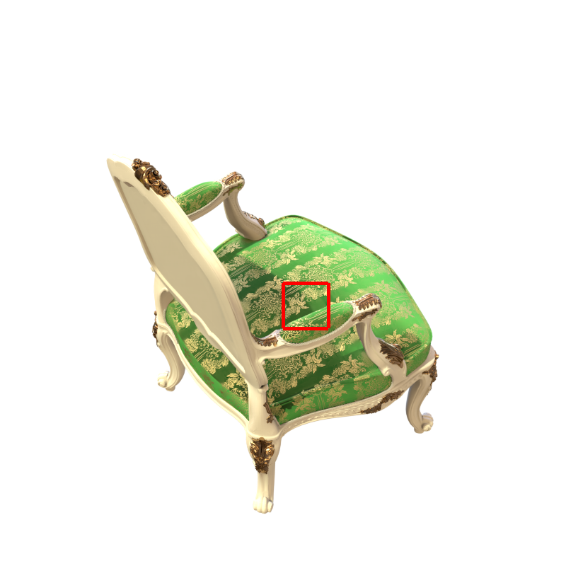
	\begin{overpic}[width=93.95122pt]{figures/multiblender_pyrs/gt_chair_15_400_400_64.png} \put(67.0,2.0){\tiny\lx@texthl@color{$$}} \put(84.0,29.0){\tiny\lx@texthl@color{$$}} \put(84.0,18.0){\tiny\lx@texthl@color{$$}} \put(76.0,10.0){\tiny\lx@texthl@color{$$}} \end{overpic}	\begin{overpic}[width=93.95122pt]{figures/multiblender_pyrs/jaxnerf_multiblender_chair_15_400_400_64.png} \put(67.0,2.0){\tiny\lx@texthl@color{$0.531$}} \put(84.0,29.0){\tiny\lx@texthl@color{$0.798$}} \put(84.0,18.0){\tiny\lx@texthl@color{$0.851$}} \put(76.0,10.0){\tiny\lx@texthl@color{$0.690$}} \end{overpic}	\begin{overpic}[width=93.95122pt]{figures/multiblender_pyrs/jaxnerf_multiblender_extras_chair_15_400_400_64.png} \put(67.0,2.0){\tiny\lx@texthl@color{$0.709$}} \put(84.0,29.0){\tiny\lx@texthl@color{$0.925$}} \put(84.0,18.0){\tiny\lx@texthl@color{$0.949$}} \put(76.0,10.0){\tiny\lx@texthl@color{$0.921$}} \end{overpic}	\begin{overpic}[width=93.95122pt]{figures/multiblender_pyrs/prenerf_multiblender_chair_15_400_400_64.png} \put(67.0,2.0){\tiny\lx@texthl@color{$\color[rgb]{0.85,0.0,0.0}0.907$}} \put(84.0,29.0){\tiny\lx@texthl@color{$\color[rgb]{0.85,0.0,0.0}0.959$}} \put(84.0,18.0){\tiny\lx@texthl@color{$\color[rgb]{0.85,0.0,0.0}0.973$}} \put(76.0,10.0){\tiny\lx@texthl@color{$\color[rgb]{0.85,0.0,0.0}0.978$}} \end{overpic}
	\begin{overpic}[width=93.95122pt]{figures/multiblender_pyrs/gt_drums_0_440_150_64.png} \put(67.0,2.0){\tiny\lx@texthl@color{$$}} \put(84.0,29.0){\tiny\lx@texthl@color{$$}} \put(84.0,18.0){\tiny\lx@texthl@color{$$}} \put(76.0,10.0){\tiny\lx@texthl@color{$$}} \end{overpic}	\begin{overpic}[width=93.95122pt]{figures/multiblender_pyrs/jaxnerf_multiblender_drums_0_440_150_64.png} \put(67.0,2.0){\tiny\lx@texthl@color{$0.709$}} \put(84.0,29.0){\tiny\lx@texthl@color{$0.910$}} \put(84.0,18.0){\tiny\lx@texthl@color{$0.931$}} \put(76.0,10.0){\tiny\lx@texthl@color{$0.663$}} \end{overpic}	\begin{overpic}[width=93.95122pt]{figures/multiblender_pyrs/jaxnerf_multiblender_extras_drums_0_440_150_64.png} \put(67.0,2.0){\tiny\lx@texthl@color{$0.863$}} \put(84.0,29.0){\tiny\lx@texthl@color{$0.959$}} \put(84.0,18.0){\tiny\lx@texthl@color{$0.971$}} \put(76.0,10.0){\tiny\lx@texthl@color{$0.881$}} \end{overpic}	\begin{overpic}[width=93.95122pt]{figures/multiblender_pyrs/prenerf_multiblender_drums_0_440_150_64.png} \put(67.0,2.0){\tiny\lx@texthl@color{$\color[rgb]{0.85,0.0,0.0}0.940$}} \put(84.0,29.0){\tiny\lx@texthl@color{$\color[rgb]{0.85,0.0,0.0}0.979$}} \put(84.0,18.0){\tiny\lx@texthl@color{$\color[rgb]{0.85,0.0,0.0}0.989$}} \put(76.0,10.0){\tiny\lx@texthl@color{$\color[rgb]{0.85,0.0,0.0}0.978$}} \end{overpic}
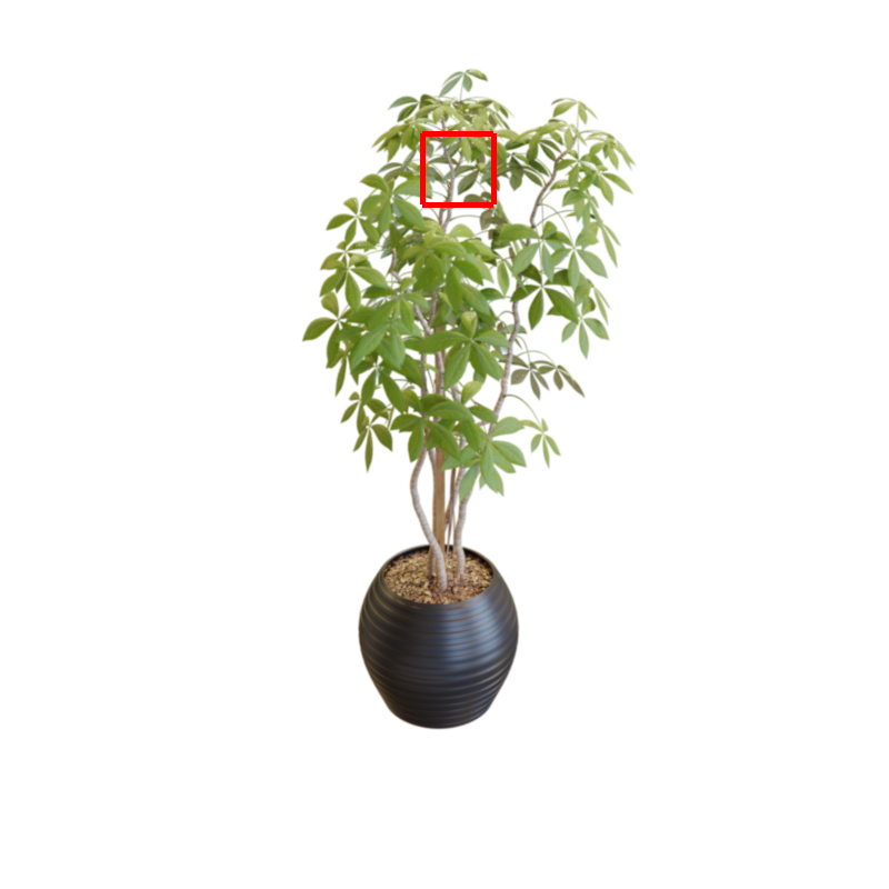
	\begin{overpic}[width=93.95122pt]{figures/multiblender_pyrs/gt_ficus_150_120_380_64.png} \put(67.0,2.0){\tiny\lx@texthl@color{$$}} \put(84.0,29.0){\tiny\lx@texthl@color{$$}} \put(84.0,18.0){\tiny\lx@texthl@color{$$}} \put(76.0,10.0){\tiny\lx@texthl@color{$$}} \end{overpic}	\begin{overpic}[width=93.95122pt]{figures/multiblender_pyrs/jaxnerf_multiblender_ficus_150_120_380_64.png} \put(67.0,2.0){\tiny\lx@texthl@color{$0.565$}} \put(84.0,29.0){\tiny\lx@texthl@color{$0.717$}} \put(84.0,18.0){\tiny\lx@texthl@color{$0.661$}} \put(76.0,10.0){\tiny\lx@texthl@color{$0.258$}} \end{overpic}	\begin{overpic}[width=93.95122pt]{figures/multiblender_pyrs/jaxnerf_multiblender_extras_ficus_150_120_380_64.png} \put(67.0,2.0){\tiny\lx@texthl@color{$0.710$}} \put(84.0,29.0){\tiny\lx@texthl@color{$0.850$}} \put(84.0,18.0){\tiny\lx@texthl@color{$0.916$}} \put(76.0,10.0){\tiny\lx@texthl@color{$0.665$}} \end{overpic}	\begin{overpic}[width=93.95122pt]{figures/multiblender_pyrs/prenerf_multiblender_ficus_150_120_380_64.png} \put(67.0,2.0){\tiny\lx@texthl@color{$\color[rgb]{0.85,0.0,0.0}0.850$}} \put(84.0,29.0){\tiny\lx@texthl@color{$\color[rgb]{0.85,0.0,0.0}0.928$}} \put(84.0,18.0){\tiny\lx@texthl@color{$\color[rgb]{0.85,0.0,0.0}0.944$}} \put(76.0,10.0){\tiny\lx@texthl@color{$\color[rgb]{0.85,0.0,0.0}0.878$}} \end{overpic}
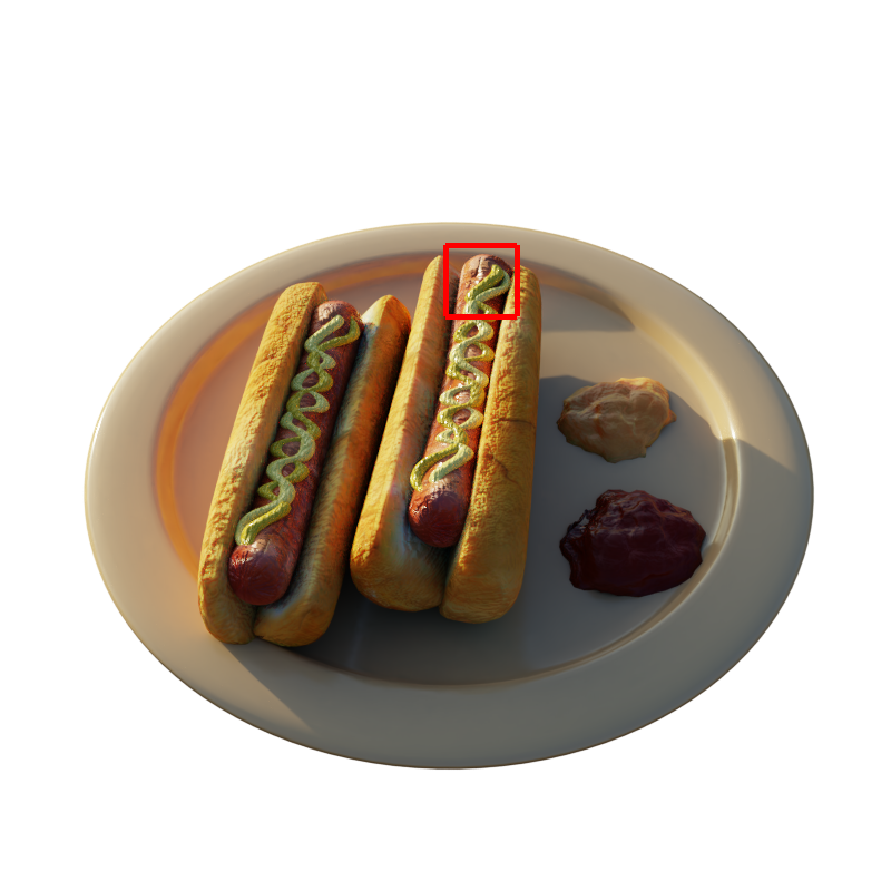
	\begin{overpic}[width=93.95122pt]{figures/multiblender_pyrs/gt_hotdog_2_220_400_64.png} \put(67.0,2.0){\tiny\lx@texthl@color{$$}} \put(84.0,29.0){\tiny\lx@texthl@color{$$}} \put(84.0,18.0){\tiny\lx@texthl@color{$$}} \put(76.0,10.0){\tiny\lx@texthl@color{$$}} \end{overpic}	\begin{overpic}[width=93.95122pt]{figures/multiblender_pyrs/jaxnerf_multiblender_hotdog_2_220_400_64.png} \put(67.0,2.0){\tiny\lx@texthl@color{$0.709$}} \put(84.0,29.0){\tiny\lx@texthl@color{$0.870$}} \put(84.0,18.0){\tiny\lx@texthl@color{$0.804$}} \put(76.0,10.0){\tiny\lx@texthl@color{$0.680$}} \end{overpic}	\begin{overpic}[width=93.95122pt]{figures/multiblender_pyrs/jaxnerf_multiblender_extras_hotdog_2_220_400_64.png} \put(67.0,2.0){\tiny\lx@texthl@color{$0.833$}} \put(84.0,29.0){\tiny\lx@texthl@color{$0.930$}} \put(84.0,18.0){\tiny\lx@texthl@color{$0.945$}} \put(76.0,10.0){\tiny\lx@texthl@color{$0.817$}} \end{overpic}	\begin{overpic}[width=93.95122pt]{figures/multiblender_pyrs/prenerf_multiblender_hotdog_2_220_400_64.png} \put(67.0,2.0){\tiny\lx@texthl@color{$\color[rgb]{0.85,0.0,0.0}0.898$}} \put(84.0,29.0){\tiny\lx@texthl@color{$\color[rgb]{0.85,0.0,0.0}0.956$}} \put(84.0,18.0){\tiny\lx@texthl@color{$\color[rgb]{0.85,0.0,0.0}0.966$}} \put(76.0,10.0){\tiny\lx@texthl@color{$\color[rgb]{0.85,0.0,0.0}0.965$}} \end{overpic}
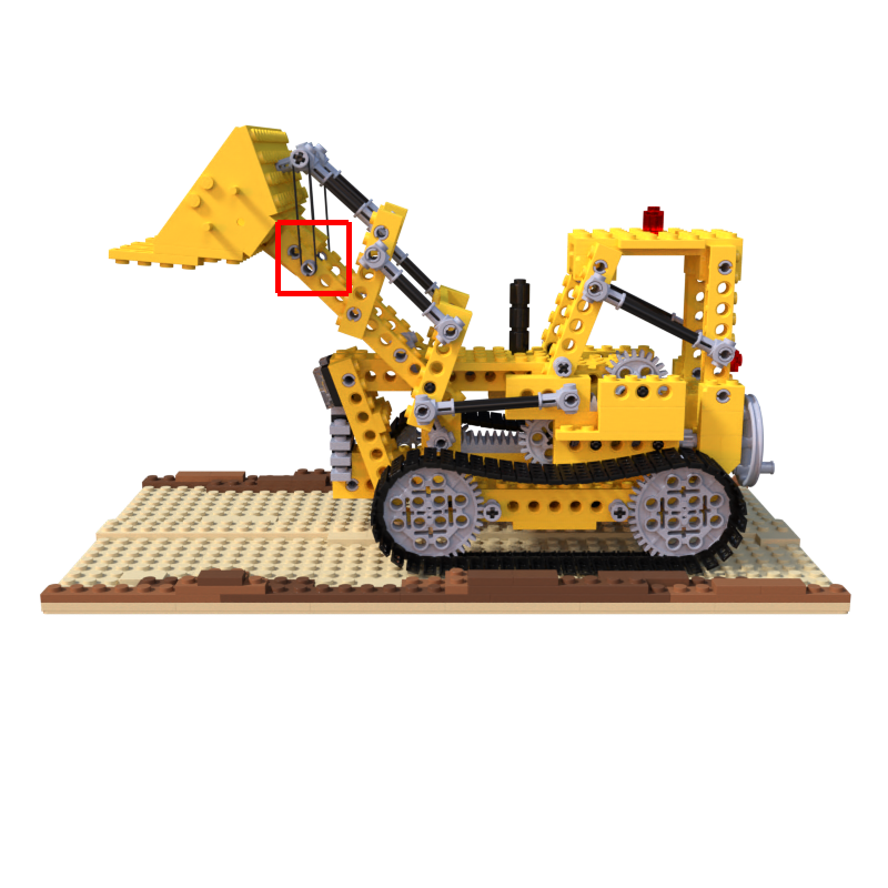
	\begin{overpic}[width=93.95122pt]{figures/multiblender_pyrs/gt_lego_75_200_250_64.png} \put(67.0,2.0){\tiny\lx@texthl@color{$$}} \put(84.0,29.0){\tiny\lx@texthl@color{$$}} \put(84.0,18.0){\tiny\lx@texthl@color{$$}} \put(76.0,10.0){\tiny\lx@texthl@color{$$}} \end{overpic}	\begin{overpic}[width=93.95122pt]{figures/multiblender_pyrs/jaxnerf_multiblender_lego_75_200_250_64.png} \put(67.0,2.0){\tiny\lx@texthl@color{$0.561$}} \put(84.0,29.0){\tiny\lx@texthl@color{$0.621$}} \put(84.0,18.0){\tiny\lx@texthl@color{$0.614$}} \put(76.0,10.0){\tiny\lx@texthl@color{$0.682$}} \end{overpic}	\begin{overpic}[width=93.95122pt]{figures/multiblender_pyrs/jaxnerf_multiblender_extras_lego_75_200_250_64.png} \put(67.0,2.0){\tiny\lx@texthl@color{$0.696$}} \put(84.0,29.0){\tiny\lx@texthl@color{$0.742$}} \put(84.0,18.0){\tiny\lx@texthl@color{$0.765$}} \put(76.0,10.0){\tiny\lx@texthl@color{$0.882$}} \end{overpic}	\begin{overpic}[width=93.95122pt]{figures/multiblender_pyrs/prenerf_multiblender_lego_75_200_250_64.png} \put(67.0,2.0){\tiny\lx@texthl@color{$\color[rgb]{0.85,0.0,0.0}0.830$}} \put(84.0,29.0){\tiny\lx@texthl@color{$\color[rgb]{0.85,0.0,0.0}0.847$}} \put(84.0,18.0){\tiny\lx@texthl@color{$\color[rgb]{0.85,0.0,0.0}0.795$}} \put(76.0,10.0){\tiny\lx@texthl@color{$\color[rgb]{0.85,0.0,0.0}0.939$}} \end{overpic}
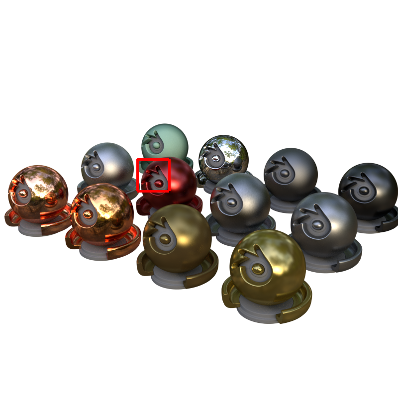
	\begin{overpic}[width=93.95122pt]{figures/multiblender_pyrs/gt_materials_60_320_276_64.png} \put(67.0,2.0){\tiny\lx@texthl@color{$$}} \put(84.0,29.0){\tiny\lx@texthl@color{$$}} \put(84.0,18.0){\tiny\lx@texthl@color{$$}} \put(76.0,10.0){\tiny\lx@texthl@color{$$}} \end{overpic}	\begin{overpic}[width=93.95122pt]{figures/multiblender_pyrs/jaxnerf_multiblender_materials_60_320_276_64.png} \put(67.0,2.0){\tiny\lx@texthl@color{$0.633$}} \put(84.0,29.0){\tiny\lx@texthl@color{$0.763$}} \put(84.0,18.0){\tiny\lx@texthl@color{$0.819$}} \put(76.0,10.0){\tiny\lx@texthl@color{$0.804$}} \end{overpic}	\begin{overpic}[width=93.95122pt]{figures/multiblender_pyrs/jaxnerf_multiblender_extras_materials_60_320_276_64.png} \put(67.0,2.0){\tiny\lx@texthl@color{$0.752$}} \put(84.0,29.0){\tiny\lx@texthl@color{$0.838$}} \put(84.0,18.0){\tiny\lx@texthl@color{$0.900$}} \put(76.0,10.0){\tiny\lx@texthl@color{$0.935$}} \end{overpic}	\begin{overpic}[width=93.95122pt]{figures/multiblender_pyrs/prenerf_multiblender_materials_60_320_276_64.png} \put(67.0,2.0){\tiny\lx@texthl@color{$\color[rgb]{0.85,0.0,0.0}0.821$}} \put(84.0,29.0){\tiny\lx@texthl@color{$\color[rgb]{0.85,0.0,0.0}0.863$}} \put(84.0,18.0){\tiny\lx@texthl@color{$\color[rgb]{0.85,0.0,0.0}0.902$}} \put(76.0,10.0){\tiny\lx@texthl@color{$\color[rgb]{0.85,0.0,0.0}0.957$}} \end{overpic}
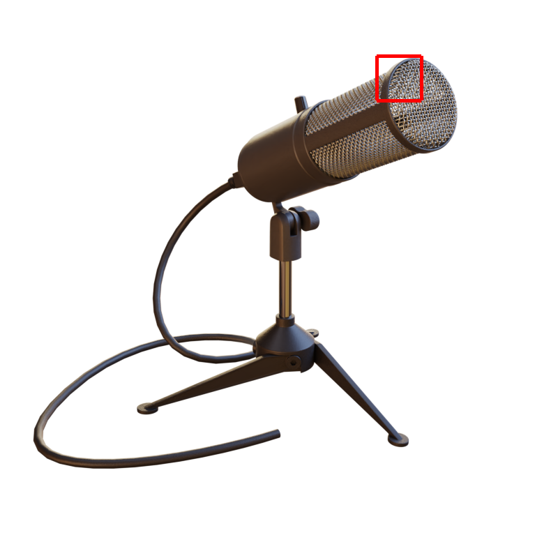
	\begin{overpic}[width=93.95122pt]{figures/multiblender_pyrs/gt_mic_140_80_540_64.png} \put(67.0,2.0){\tiny\lx@texthl@color{$$}} \put(84.0,29.0){\tiny\lx@texthl@color{$$}} \put(84.0,18.0){\tiny\lx@texthl@color{$$}} \put(76.0,10.0){\tiny\lx@texthl@color{$$}} \end{overpic}	\begin{overpic}[width=93.95122pt]{figures/multiblender_pyrs/jaxnerf_multiblender_mic_140_80_540_64.png} \put(67.0,2.0){\tiny\lx@texthl@color{$0.425$}} \put(84.0,29.0){\tiny\lx@texthl@color{$0.600$}} \put(84.0,18.0){\tiny\lx@texthl@color{$0.739$}} \put(76.0,10.0){\tiny\lx@texthl@color{$0.838$}} \end{overpic}	\begin{overpic}[width=93.95122pt]{figures/multiblender_pyrs/jaxnerf_multiblender_extras_mic_140_80_540_64.png} \put(67.0,2.0){\tiny\lx@texthl@color{$0.566$}} \put(84.0,29.0){\tiny\lx@texthl@color{$0.745$}} \put(84.0,18.0){\tiny\lx@texthl@color{$0.776$}} \put(76.0,10.0){\tiny\lx@texthl@color{$0.924$}} \end{overpic}	\begin{overpic}[width=93.95122pt]{figures/multiblender_pyrs/prenerf_multiblender_mic_140_80_540_64.png} \put(67.0,2.0){\tiny\lx@texthl@color{$\color[rgb]{0.85,0.0,0.0}0.793$}} \put(84.0,29.0){\tiny\lx@texthl@color{$\color[rgb]{0.85,0.0,0.0}0.844$}} \put(84.0,18.0){\tiny\lx@texthl@color{$\color[rgb]{0.85,0.0,0.0}0.846$}} \put(76.0,10.0){\tiny\lx@texthl@color{$\color[rgb]{0.85,0.0,0.0}0.987$}} \end{overpic}
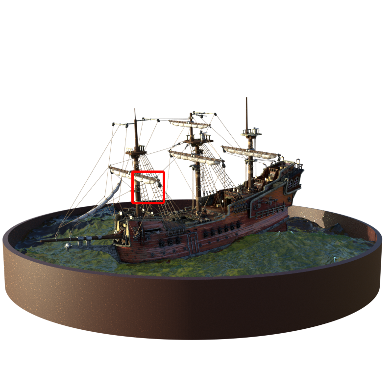
	\begin{overpic}[width=93.95122pt]{figures/multiblender_pyrs/gt_ship_90_350_270_64.png} \put(67.0,2.0){\tiny\lx@texthl@color{$$}} \put(84.0,29.0){\tiny\lx@texthl@color{$$}} \put(84.0,18.0){\tiny\lx@texthl@color{$$}} \put(76.0,10.0){\tiny\lx@texthl@color{$$}} \end{overpic}	\begin{overpic}[width=93.95122pt]{figures/multiblender_pyrs/jaxnerf_multiblender_ship_90_350_270_64.png} \put(67.0,2.0){\tiny\lx@texthl@color{$0.420$}} \put(84.0,29.0){\tiny\lx@texthl@color{$0.618$}} \put(84.0,18.0){\tiny\lx@texthl@color{$0.723$}} \put(76.0,10.0){\tiny\lx@texthl@color{$0.755$}} \end{overpic}	\begin{overpic}[width=93.95122pt]{figures/multiblender_pyrs/jaxnerf_multiblender_extras_ship_90_350_270_64.png} \put(67.0,2.0){\tiny\lx@texthl@color{$0.584$}} \put(84.0,29.0){\tiny\lx@texthl@color{$0.810$}} \put(84.0,18.0){\tiny\lx@texthl@color{$0.937$}} \put(76.0,10.0){\tiny\lx@texthl@color{$0.907$}} \end{overpic}	\begin{overpic}[width=93.95122pt]{figures/multiblender_pyrs/prenerf_multiblender_ship_90_350_270_64.png} \put(67.0,2.0){\tiny\lx@texthl@color{$\color[rgb]{0.85,0.0,0.0}0.823$}} \put(84.0,29.0){\tiny\lx@texthl@color{$\color[rgb]{0.85,0.0,0.0}0.929$}} \put(84.0,18.0){\tiny\lx@texthl@color{$\color[rgb]{0.85,0.0,0.0}0.963$}} \put(76.0,10.0){\tiny\lx@texthl@color{$\color[rgb]{0.85,0.0,0.0}0.968$}} \end{overpic}
Ground-Truth		NeRF	NeRF + Area, Center, Misc	Mip-NeRF

Figure 9: Visualizations of the output renderings from mip-NeRF compared to the ground truth, NeRF, and our improved version of NeRF, on test set images from the 8 scenes in our multiscale Blender dataset. We visualize a cropped region of each scene for better visualization, and render out that scene at 4 different resolutions, displayed as an image pyramid. The SSIM for each scale of each image pyramid truth is shown to its lower right, with the highest SSIM for each algorithm at each scale highlighted in red.

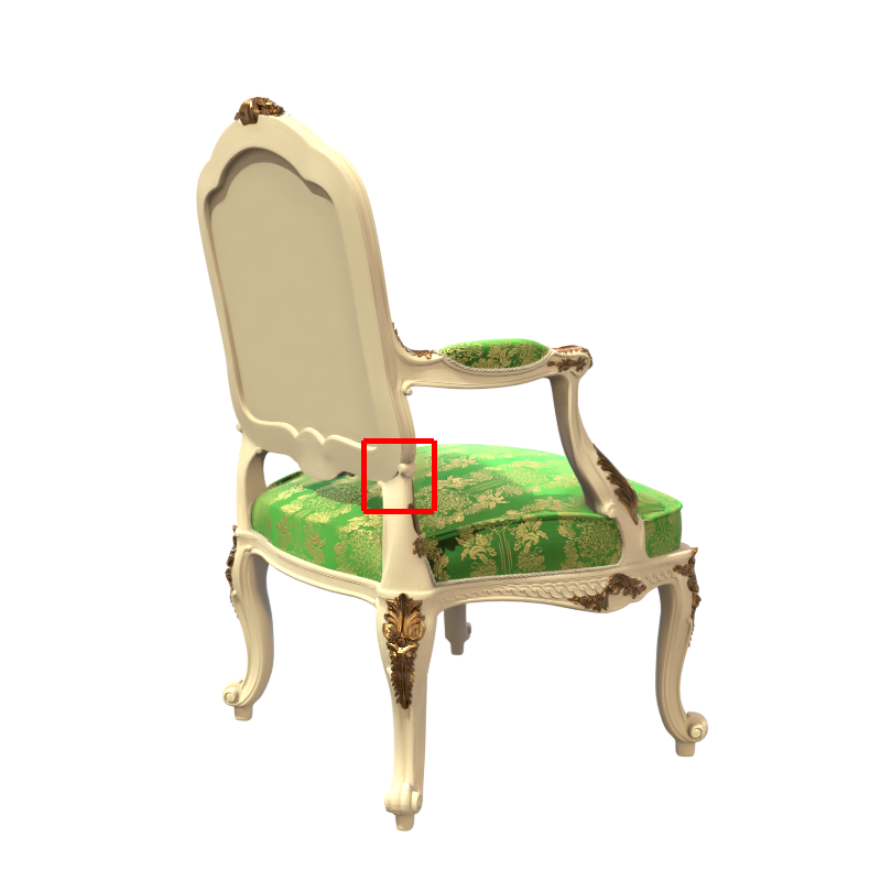
	\begin{overpic}[width=93.95122pt]{figures/multiblender_pyrs/gt_chair_115_400_330_64.png} \put(67.0,2.0){\tiny\lx@texthl@color{$$}} \put(84.0,29.0){\tiny\lx@texthl@color{$$}} \put(84.0,18.0){\tiny\lx@texthl@color{$$}} \put(76.0,10.0){\tiny\lx@texthl@color{$$}} \end{overpic}	\begin{overpic}[width=93.95122pt]{figures/multiblender_pyrs/jaxnerf_multiblender_chair_115_400_330_64.png} \put(67.0,2.0){\tiny\lx@texthl@color{$0.758$}} \put(84.0,29.0){\tiny\lx@texthl@color{$0.857$}} \put(84.0,18.0){\tiny\lx@texthl@color{$0.904$}} \put(76.0,10.0){\tiny\lx@texthl@color{$0.850$}} \end{overpic}	\begin{overpic}[width=93.95122pt]{figures/multiblender_pyrs/jaxnerf_multiblender_extras_chair_115_400_330_64.png} \put(67.0,2.0){\tiny\lx@texthl@color{$0.844$}} \put(84.0,29.0){\tiny\lx@texthl@color{$0.918$}} \put(84.0,18.0){\tiny\lx@texthl@color{$0.964$}} \put(76.0,10.0){\tiny\lx@texthl@color{$0.941$}} \end{overpic}	\begin{overpic}[width=93.95122pt]{figures/multiblender_pyrs/prenerf_multiblender_chair_115_400_330_64.png} \put(67.0,2.0){\tiny\lx@texthl@color{$\color[rgb]{0.85,0.0,0.0}0.863$}} \put(84.0,29.0){\tiny\lx@texthl@color{$\color[rgb]{0.85,0.0,0.0}0.923$}} \put(84.0,18.0){\tiny\lx@texthl@color{$\color[rgb]{0.85,0.0,0.0}0.970$}} \put(76.0,10.0){\tiny\lx@texthl@color{$\color[rgb]{0.85,0.0,0.0}0.967$}} \end{overpic}
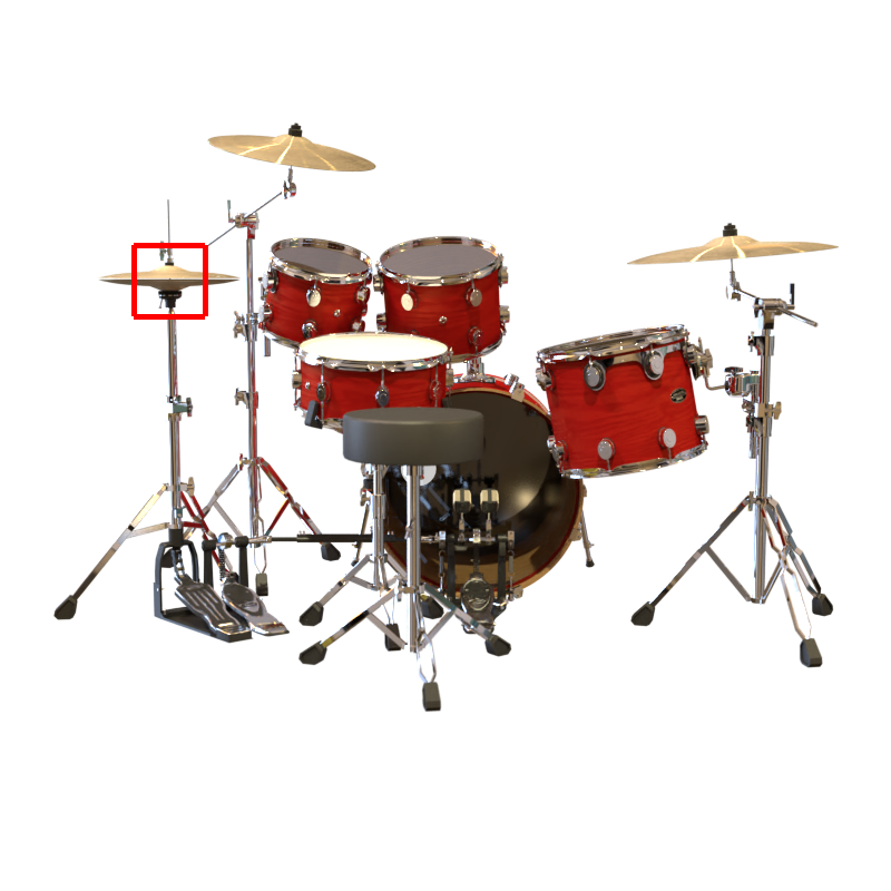
	\begin{overpic}[width=93.95122pt]{figures/multiblender_pyrs/gt_drums_100_220_120_64.png} \put(67.0,2.0){\tiny\lx@texthl@color{$$}} \put(84.0,29.0){\tiny\lx@texthl@color{$$}} \put(84.0,18.0){\tiny\lx@texthl@color{$$}} \put(76.0,10.0){\tiny\lx@texthl@color{$$}} \end{overpic}	\begin{overpic}[width=93.95122pt]{figures/multiblender_pyrs/jaxnerf_multiblender_drums_100_220_120_64.png} \put(67.0,2.0){\tiny\lx@texthl@color{$0.665$}} \put(84.0,29.0){\tiny\lx@texthl@color{$0.804$}} \put(84.0,18.0){\tiny\lx@texthl@color{$\color[rgb]{0.85,0.0,0.0}0.918$}} \put(76.0,10.0){\tiny\lx@texthl@color{$0.814$}} \end{overpic}	\begin{overpic}[width=93.95122pt]{figures/multiblender_pyrs/jaxnerf_multiblender_extras_drums_100_220_120_64.png} \put(67.0,2.0){\tiny\lx@texthl@color{$0.721$}} \put(84.0,29.0){\tiny\lx@texthl@color{$0.825$}} \put(84.0,18.0){\tiny\lx@texthl@color{$0.913$}} \put(76.0,10.0){\tiny\lx@texthl@color{$0.896$}} \end{overpic}	\begin{overpic}[width=93.95122pt]{figures/multiblender_pyrs/prenerf_multiblender_drums_100_220_120_64.png} \put(67.0,2.0){\tiny\lx@texthl@color{$\color[rgb]{0.85,0.0,0.0}0.771$}} \put(84.0,29.0){\tiny\lx@texthl@color{$\color[rgb]{0.85,0.0,0.0}0.846$}} \put(84.0,18.0){\tiny\lx@texthl@color{$0.915$}} \put(76.0,10.0){\tiny\lx@texthl@color{$\color[rgb]{0.85,0.0,0.0}0.910$}} \end{overpic}
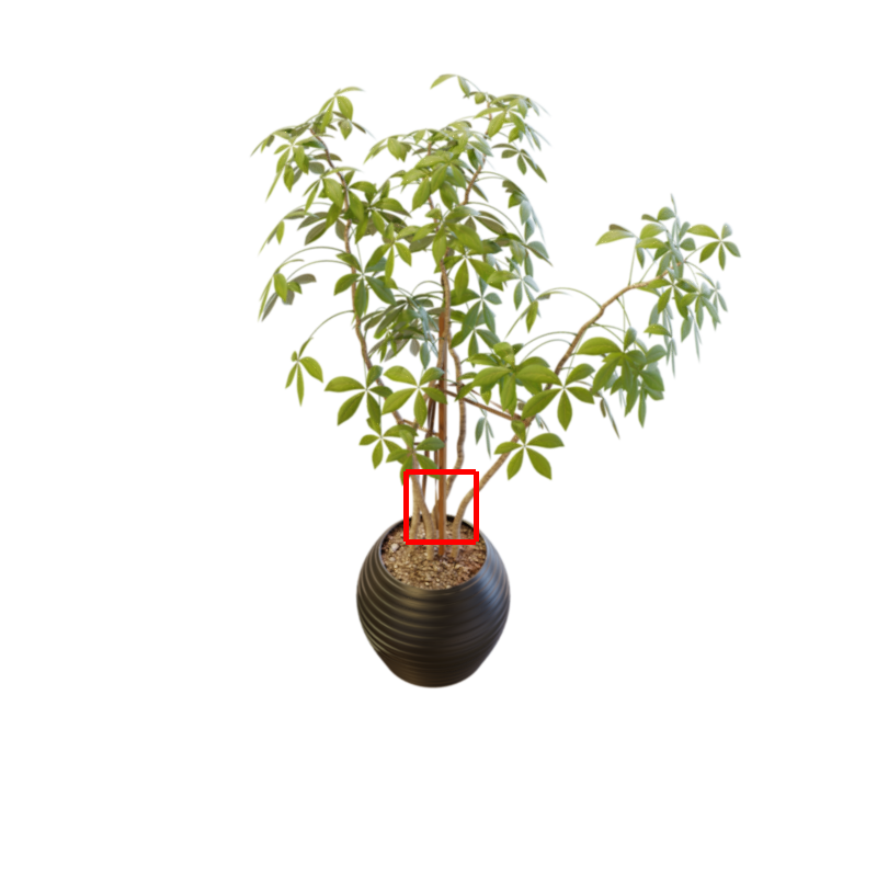
	\begin{overpic}[width=93.95122pt]{figures/multiblender_pyrs/gt_ficus_30_430_370_64.png} \put(67.0,2.0){\tiny\lx@texthl@color{$$}} \put(84.0,29.0){\tiny\lx@texthl@color{$$}} \put(84.0,18.0){\tiny\lx@texthl@color{$$}} \put(76.0,10.0){\tiny\lx@texthl@color{$$}} \end{overpic}	\begin{overpic}[width=93.95122pt]{figures/multiblender_pyrs/jaxnerf_multiblender_ficus_30_430_370_64.png} \put(67.0,2.0){\tiny\lx@texthl@color{$0.685$}} \put(84.0,29.0){\tiny\lx@texthl@color{$0.832$}} \put(84.0,18.0){\tiny\lx@texthl@color{$0.874$}} \put(76.0,10.0){\tiny\lx@texthl@color{$0.779$}} \end{overpic}	\begin{overpic}[width=93.95122pt]{figures/multiblender_pyrs/jaxnerf_multiblender_extras_ficus_30_430_370_64.png} \put(67.0,2.0){\tiny\lx@texthl@color{$0.868$}} \put(84.0,29.0){\tiny\lx@texthl@color{$0.949$}} \put(84.0,18.0){\tiny\lx@texthl@color{$0.971$}} \put(76.0,10.0){\tiny\lx@texthl@color{$0.929$}} \end{overpic}	\begin{overpic}[width=93.95122pt]{figures/multiblender_pyrs/prenerf_multiblender_ficus_30_430_370_64.png} \put(67.0,2.0){\tiny\lx@texthl@color{$\color[rgb]{0.85,0.0,0.0}0.922$}} \put(84.0,29.0){\tiny\lx@texthl@color{$\color[rgb]{0.85,0.0,0.0}0.960$}} \put(84.0,18.0){\tiny\lx@texthl@color{$\color[rgb]{0.85,0.0,0.0}0.973$}} \put(76.0,10.0){\tiny\lx@texthl@color{$\color[rgb]{0.85,0.0,0.0}0.971$}} \end{overpic}
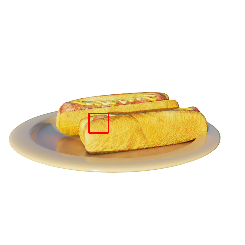
	\begin{overpic}[width=93.95122pt]{figures/multiblender_pyrs/gt_hotdog_70_370_290_64.png} \put(67.0,2.0){\tiny\lx@texthl@color{$$}} \put(84.0,29.0){\tiny\lx@texthl@color{$$}} \put(84.0,18.0){\tiny\lx@texthl@color{$$}} \put(76.0,10.0){\tiny\lx@texthl@color{$$}} \end{overpic}	\begin{overpic}[width=93.95122pt]{figures/multiblender_pyrs/jaxnerf_multiblender_hotdog_70_370_290_64.png} \put(67.0,2.0){\tiny\lx@texthl@color{$0.659$}} \put(84.0,29.0){\tiny\lx@texthl@color{$0.794$}} \put(84.0,18.0){\tiny\lx@texthl@color{$0.890$}} \put(76.0,10.0){\tiny\lx@texthl@color{$0.763$}} \end{overpic}	\begin{overpic}[width=93.95122pt]{figures/multiblender_pyrs/jaxnerf_multiblender_extras_hotdog_70_370_290_64.png} \put(67.0,2.0){\tiny\lx@texthl@color{$0.743$}} \put(84.0,29.0){\tiny\lx@texthl@color{$0.863$}} \put(84.0,18.0){\tiny\lx@texthl@color{$0.942$}} \put(76.0,10.0){\tiny\lx@texthl@color{$0.906$}} \end{overpic}	\begin{overpic}[width=93.95122pt]{figures/multiblender_pyrs/prenerf_multiblender_hotdog_70_370_290_64.png} \put(67.0,2.0){\tiny\lx@texthl@color{$\color[rgb]{0.85,0.0,0.0}0.864$}} \put(84.0,29.0){\tiny\lx@texthl@color{$\color[rgb]{0.85,0.0,0.0}0.935$}} \put(84.0,18.0){\tiny\lx@texthl@color{$\color[rgb]{0.85,0.0,0.0}0.965$}} \put(76.0,10.0){\tiny\lx@texthl@color{$\color[rgb]{0.85,0.0,0.0}0.966$}} \end{overpic}
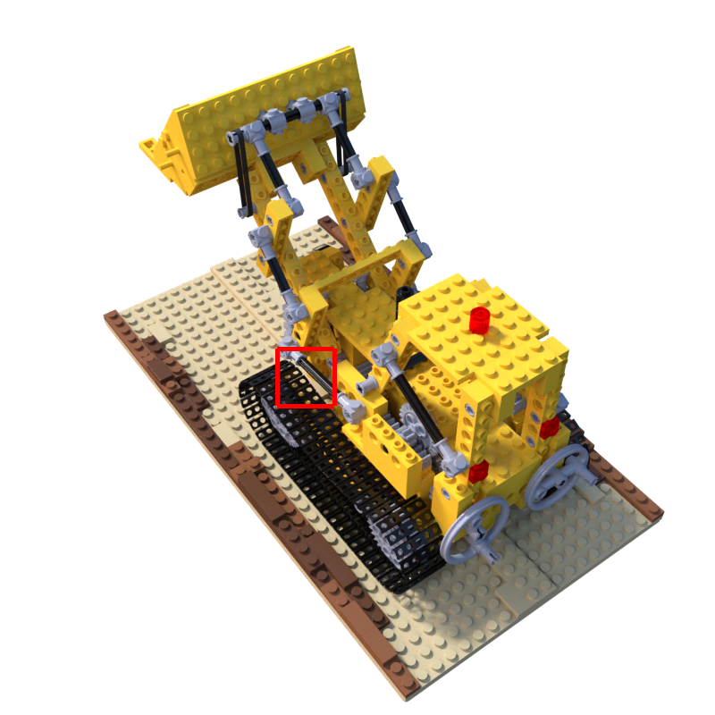
	\begin{overpic}[width=93.95122pt]{figures/multiblender_pyrs/gt_lego_190_390_310_64.png} \put(67.0,2.0){\tiny\lx@texthl@color{$$}} \put(84.0,29.0){\tiny\lx@texthl@color{$$}} \put(84.0,18.0){\tiny\lx@texthl@color{$$}} \put(76.0,10.0){\tiny\lx@texthl@color{$$}} \end{overpic}	\begin{overpic}[width=93.95122pt]{figures/multiblender_pyrs/jaxnerf_multiblender_lego_190_390_310_64.png} \put(67.0,2.0){\tiny\lx@texthl@color{$0.542$}} \put(84.0,29.0){\tiny\lx@texthl@color{$0.668$}} \put(84.0,18.0){\tiny\lx@texthl@color{$0.701$}} \put(76.0,10.0){\tiny\lx@texthl@color{$0.734$}} \end{overpic}	\begin{overpic}[width=93.95122pt]{figures/multiblender_pyrs/jaxnerf_multiblender_extras_lego_190_390_310_64.png} \put(67.0,2.0){\tiny\lx@texthl@color{$0.720$}} \put(84.0,29.0){\tiny\lx@texthl@color{$0.843$}} \put(84.0,18.0){\tiny\lx@texthl@color{$0.910$}} \put(76.0,10.0){\tiny\lx@texthl@color{$0.747$}} \end{overpic}	\begin{overpic}[width=93.95122pt]{figures/multiblender_pyrs/prenerf_multiblender_lego_190_390_310_64.png} \put(67.0,2.0){\tiny\lx@texthl@color{$\color[rgb]{0.85,0.0,0.0}0.824$}} \put(84.0,29.0){\tiny\lx@texthl@color{$\color[rgb]{0.85,0.0,0.0}0.901$}} \put(84.0,18.0){\tiny\lx@texthl@color{$\color[rgb]{0.85,0.0,0.0}0.940$}} \put(76.0,10.0){\tiny\lx@texthl@color{$\color[rgb]{0.85,0.0,0.0}0.923$}} \end{overpic}
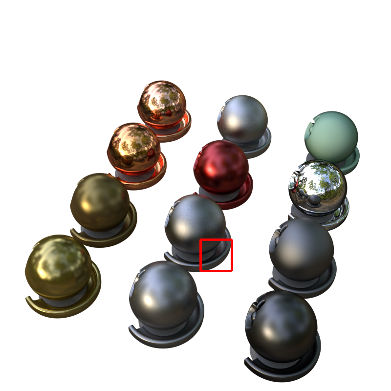
	\begin{overpic}[width=93.95122pt]{figures/multiblender_pyrs/gt_materials_180_490_410_64.png} \put(67.0,2.0){\tiny\lx@texthl@color{$$}} \put(84.0,29.0){\tiny\lx@texthl@color{$$}} \put(84.0,18.0){\tiny\lx@texthl@color{$$}} \put(76.0,10.0){\tiny\lx@texthl@color{$$}} \end{overpic}	\begin{overpic}[width=93.95122pt]{figures/multiblender_pyrs/jaxnerf_multiblender_materials_180_490_410_64.png} \put(67.0,2.0){\tiny\lx@texthl@color{$0.733$}} \put(84.0,29.0){\tiny\lx@texthl@color{$0.832$}} \put(84.0,18.0){\tiny\lx@texthl@color{$0.838$}} \put(76.0,10.0){\tiny\lx@texthl@color{$0.787$}} \end{overpic}	\begin{overpic}[width=93.95122pt]{figures/multiblender_pyrs/jaxnerf_multiblender_extras_materials_180_490_410_64.png} \put(67.0,2.0){\tiny\lx@texthl@color{$0.879$}} \put(84.0,29.0){\tiny\lx@texthl@color{$0.926$}} \put(84.0,18.0){\tiny\lx@texthl@color{$0.946$}} \put(76.0,10.0){\tiny\lx@texthl@color{$0.971$}} \end{overpic}	\begin{overpic}[width=93.95122pt]{figures/multiblender_pyrs/prenerf_multiblender_materials_180_490_410_64.png} \put(67.0,2.0){\tiny\lx@texthl@color{$\color[rgb]{0.85,0.0,0.0}0.935$}} \put(84.0,29.0){\tiny\lx@texthl@color{$\color[rgb]{0.85,0.0,0.0}0.964$}} \put(84.0,18.0){\tiny\lx@texthl@color{$\color[rgb]{0.85,0.0,0.0}0.975$}} \put(76.0,10.0){\tiny\lx@texthl@color{$\color[rgb]{0.85,0.0,0.0}0.994$}} \end{overpic}
	\begin{overpic}[width=93.95122pt]{figures/multiblender_pyrs/gt_mic_120_80_560_64.png} \put(67.0,2.0){\tiny\lx@texthl@color{$$}} \put(84.0,29.0){\tiny\lx@texthl@color{$$}} \put(84.0,18.0){\tiny\lx@texthl@color{$$}} \put(76.0,10.0){\tiny\lx@texthl@color{$$}} \end{overpic}	\begin{overpic}[width=93.95122pt]{figures/multiblender_pyrs/jaxnerf_multiblender_mic_120_80_560_64.png} \put(67.0,2.0){\tiny\lx@texthl@color{$0.448$}} \put(84.0,29.0){\tiny\lx@texthl@color{$0.562$}} \put(84.0,18.0){\tiny\lx@texthl@color{$0.696$}} \put(76.0,10.0){\tiny\lx@texthl@color{$0.906$}} \end{overpic}	\begin{overpic}[width=93.95122pt]{figures/multiblender_pyrs/jaxnerf_multiblender_extras_mic_120_80_560_64.png} \put(67.0,2.0){\tiny\lx@texthl@color{$0.525$}} \put(84.0,29.0){\tiny\lx@texthl@color{$0.633$}} \put(84.0,18.0){\tiny\lx@texthl@color{$0.794$}} \put(76.0,10.0){\tiny\lx@texthl@color{$0.918$}} \end{overpic}	\begin{overpic}[width=93.95122pt]{figures/multiblender_pyrs/prenerf_multiblender_mic_120_80_560_64.png} \put(67.0,2.0){\tiny\lx@texthl@color{$\color[rgb]{0.85,0.0,0.0}0.785$}} \put(84.0,29.0){\tiny\lx@texthl@color{$\color[rgb]{0.85,0.0,0.0}0.837$}} \put(84.0,18.0){\tiny\lx@texthl@color{$\color[rgb]{0.85,0.0,0.0}0.861$}} \put(76.0,10.0){\tiny\lx@texthl@color{$\color[rgb]{0.85,0.0,0.0}0.975$}} \end{overpic}
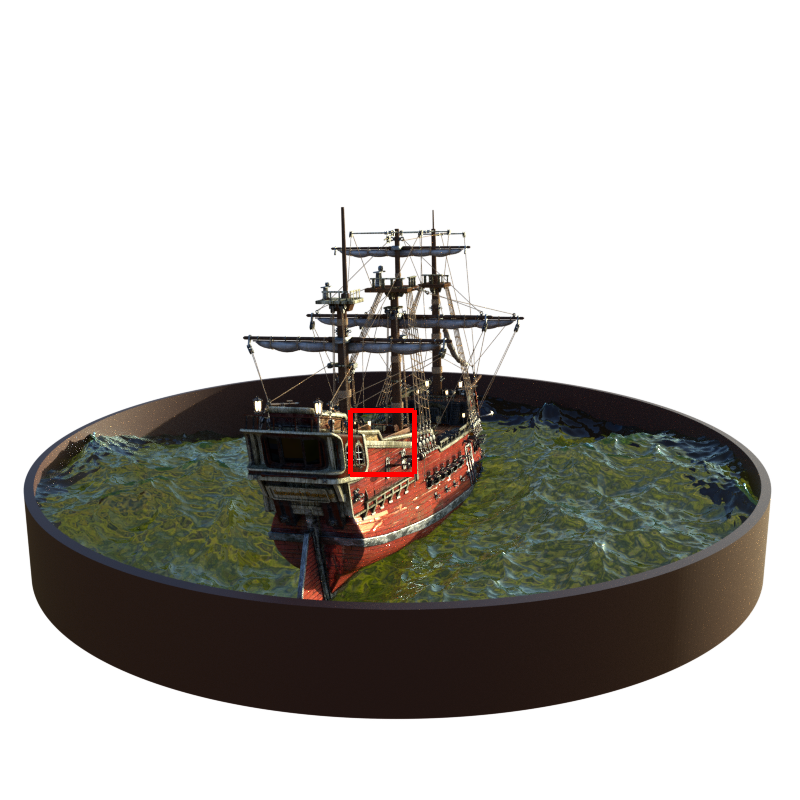
	\begin{overpic}[width=93.95122pt]{figures/multiblender_pyrs/gt_ship_130_410_350_64.png} \put(67.0,2.0){\tiny\lx@texthl@color{$$}} \put(84.0,29.0){\tiny\lx@texthl@color{$$}} \put(84.0,18.0){\tiny\lx@texthl@color{$$}} \put(76.0,10.0){\tiny\lx@texthl@color{$$}} \end{overpic}	\begin{overpic}[width=93.95122pt]{figures/multiblender_pyrs/jaxnerf_multiblender_ship_130_410_350_64.png} \put(67.0,2.0){\tiny\lx@texthl@color{$0.494$}} \put(84.0,29.0){\tiny\lx@texthl@color{$0.742$}} \put(84.0,18.0){\tiny\lx@texthl@color{$0.839$}} \put(76.0,10.0){\tiny\lx@texthl@color{$0.810$}} \end{overpic}	\begin{overpic}[width=93.95122pt]{figures/multiblender_pyrs/jaxnerf_multiblender_extras_ship_130_410_350_64.png} \put(67.0,2.0){\tiny\lx@texthl@color{$0.655$}} \put(84.0,29.0){\tiny\lx@texthl@color{$0.859$}} \put(84.0,18.0){\tiny\lx@texthl@color{$0.944$}} \put(76.0,10.0){\tiny\lx@texthl@color{$0.833$}} \end{overpic}	\begin{overpic}[width=93.95122pt]{figures/multiblender_pyrs/prenerf_multiblender_ship_130_410_350_64.png} \put(67.0,2.0){\tiny\lx@texthl@color{$\color[rgb]{0.85,0.0,0.0}0.790$}} \put(84.0,29.0){\tiny\lx@texthl@color{$\color[rgb]{0.85,0.0,0.0}0.915$}} \put(84.0,18.0){\tiny\lx@texthl@color{$\color[rgb]{0.85,0.0,0.0}0.967$}} \put(76.0,10.0){\tiny\lx@texthl@color{$\color[rgb]{0.85,0.0,0.0}0.972$}} \end{overpic}
Ground-Truth		NeRF	NeRF + Area, Center, Misc	Mip-NeRF

Figure 10: Additional visualizations of the output renderings from mip-NeRF compared to the ground truth, NeRF, and an improved version of NeRF presented in this work, on test set images from the 8 scenes in our multiscale Blender dataset, in the same format as Figure 9.

SSIM    chair drums ficus hotdog lego materials mic ship SRN [srn] 0.910 0.766 0.849 0.923 0.809 0.808 0.947 0.757 Neural Volumes [neuralvolumes] 0.916 0.873 0.910 0.944 0.880 0.888 0.946 0.784 LLFF [mildenhall2019] 0.948 0.890 0.896 0.965 0.911 0.890 0.964 0.823 NSVF [liu2020neural] 0.968 0.931 0.973 0.980 0.960 0.973 0.987 0.854 NeRF (TF Implementation) [mildenhall2020] 0.967 0.925 0.964 0.974 0.961 0.949 0.980 0.856 NeRF (Jax Implementation) [jaxnerf2020github, mildenhall2020] 0.975 0.925 0.967 0.979 0.968 0.953 0.987 0.869 NeRF + Centered Pixels 0.979 0.928 0.971 0.980 0.973 0.956 0.989 0.877 NeRF + Center, Misc. 0.979 0.927 0.971 0.980 0.972 0.956 0.989 0.877 Mip-NeRF 0.981 0.932 0.980 0.982 0.978 0.959 0.991 0.882 Mip-NeRF w/o Single MLP 0.980 0.929 0.977 0.981 0.976 0.956 0.989 0.883 Mip-NeRF w/o Misc. 0.981 0.932 0.979 0.982 0.978 0.959 0.991 0.883 Mip-NeRF w/o IPE 0.981 0.929 0.972 0.981 0.975 0.958 0.990 0.878 Mip-NeRF, Stopped Early 0.976 0.927 0.969 0.979 0.969 0.954 0.988 0.869          LPIPS    chair drums ficus hotdog lego materials mic ship SRN [srn] 0.106 0.267 0.149 0.100 0.200 0.174 0.063 0.299 Neural Volumes [neuralvolumes] 0.109 0.214 0.162 0.109 0.175 0.130 0.107 0.276 LLFF [mildenhall2019] 0.064 0.126 0.130 0.061 0.110 0.117 0.084 0.218 NSVF [liu2020neural] 0.043 0.069 0.017 0.025 0.029 0.021 0.010 0.162 NeRF (TF Implementation) [mildenhall2020] 0.046 0.091 0.044 0.121 0.050 0.063 0.028 0.206 NeRF (Jax Implementation) [jaxnerf2020github, mildenhall2020] 0.026 0.071 0.032 0.030 0.031 0.047 0.012 0.150 NeRF + Centered Pixels 0.022 0.069 0.028 0.028 0.026 0.043 0.010 0.143 NeRF + Center, Misc. 0.022 0.069 0.028 0.028 0.027 0.044 0.011 0.142 Mip-NeRF 0.021 0.065 0.020 0.027 0.021 0.040 0.009 0.138 Mip-NeRF w/o Single MLP 0.022 0.067 0.023 0.028 0.024 0.044 0.011 0.135 Mip-NeRF w/o Misc. 0.021 0.066 0.022 0.026 0.021 0.040 0.009 0.136 Mip-NeRF w/o IPE 0.020 0.068 0.027 0.028 0.024 0.041 0.009 0.142 Mip-NeRF, Stopped Early 0.027 0.074 0.035 0.031 0.035 0.046 0.013 0.155

Table 7: Per-scene results on the test set images of the (single-scale) Blender dataset from Mildenhall et al. [mildenhall2020]