Scalable Pareto Front Approximation for Deep Multi-Objective Learning

Abstract

Multi-objective optimization (MOO) is a prevalent challenge for Deep Learning, however, there exists no scalable MOO solution for truly deep neural networks. Prior work either demand optimizing a new network for every point on the Pareto front, or induce a large overhead to the number of trainable parameters by using hyper-networks conditioned on modifiable preferences. In this paper, we propose to condition the network directly on these preferences by augmenting them to the feature space. Furthermore, we ensure a well-spread Pareto front by penalizing the solutions to maintain a small angle to the preference vector. In a series of experiments, we demonstrate that our Pareto fronts achieve state-of-the-art quality despite being computed significantly faster. Furthermore, we showcase the scalability as our method approximates the full Pareto front on the CelebA dataset with an EfficientNet network at a tiny training time overhead of 7% compared to a simple single-objective optimization. We will make our code publicly available.

1 Introduction

Multi-objective optimization (MOO) is a pillar task for Machine Learning and manifests itself in numerous real-life problems, such as multi-task learning (MTL) or fair machine learning which jointly minimizes both the classification error and at least one fairness criterion. MOO is a classical problem in operations research and is typically solved through evolutionary methods, however, it recently gained interest in the Machine Learning community thanks to the development of new gradient-based MOO algorithms that facilitate faster training times (Fliege & Svaiter, 2000; Désidéri, 2012). The goal of MOO is to generate a Pareto front of non-dominating solutions, in a way that a practitioner selects a post hoc solution based on the achieved trade-offs among objectives. The Pareto front denotes a set of solutions which cannot be further optimized without sacrificing performance with respect to at least one objective, its elements are called pareto-optimal (see Section 3).

The earlier attempt to tackle MOO for Deep Learning focused on addressing multi-task learning (Sener & Koltun, 2018) through gradient descent (Désidéri, 2012) to find a single solution on the Pareto front. Additional follow-up strategies propose to populate a set of Pareto optimal solutions by learning multiple neural networks along preference vectors (Lin et al., 2019; Mahapatra & Rajan, 2020). Preference vectors encode the predefined relative importance for each objective. Two recent ideas proposed conditioning the network’s weights to the preference vector through hyper-networks (Lin et al., 2021; Navon et al., 2021). A key problem with the aforementioned prior work is that they struggle to scale to deep neural networks. Learning one new network for each Pareto front solution makes it infeasible to populate a large set, while the overhead of the hyper-networks is prohibitive in terms of increasing the number of trainable parameters.

In this paper we propose a novel method that scales MOO to Deep Learning by fulfilling two important desiderata: $i)$ our method does not significantly increase the trainable parameters of the network (contrary to hyper-networks), and $ii)$ generates the full Pareto front of solutions in a single optimization run (contrary to methods that train one network per point in the Pareto front). Concretely, we propose to condition a prediction model to the choice of the preference vectors by augmenting the feature space with the preferences. As a consequence, our method learns to adapt a single network for all the trade-off combinations of the inputted preference vectors, therefore it is able to approximate all solutions of the Pareto front after a single optimization run. We follow the linear scalarization variant of MOO, which although is the fastest variant for gradient-based learning, does not produce a well-spread Pareto front (Mahapatra & Rajan, 2020; Navon et al., 2021; Lin et al., 2019). To remedy this disadvantage, we propose a novel penalty term that forces the achieved solutions in the objectives’ space to maintain a small angle to the inputted preference vector.

In a series of experiments, we demonstrate that our method competes strongly with the state-of-the-art MOO methods in terms of quality while being significantly faster. To further showcase the efficiency of our technique, we demonstrate that it is feasible to efficiently approximate the Pareto front by fine-tuning a deep network on a large-scale multi-objective problem within less than 4 GPU hours. To sum up, this paper introduces the following contributions:

1. A novel method for MOO in Deep Learning that needs a single optimization run to approximate the full set of the Pareto front;

2. Conditioning the model to the preference vectors on the feature space, removing the overhead of hyper-networks on the number of trainable parameters;

3. A novel penalty term to enforce that the Pareto front achieved through linear scalarization is well-spread across the objectives’ space;

4. Experimental results showing our method is an efficient MOO approach that approximates a Pareto front for deep models on large multi-objective datasets at negligible training time overhead of 7% compared to a single-objective optimization.

2 Related Work

Multi-Task Learning refers to learning a prediction model for solving multiple tasks jointly and is applicable in various application domains (Zhang & Yang, 2018), for instance in detecting facial landmarks on images (Zhang et al., 2014). Tasks can have competing objectives, and finding the right balance for prioritizing them is challenging. A prior work explores mechanisms for deciding which tasks should be prioritized (Standley et al., 2020). Furthermore, the adaptive load balancing of competing losses has also attracted interest (Chen et al., 2018). On the other hand, a tailored architecture for addressing multi-task involved task-specific feature-level attention (Liu et al., 2019). Besides, a prior work explores the direction of modeling uncertainty for multi-task learning (Kendall et al., 2018).

Multi-Objective Optimization formalizes the problem of learning from multiple objectives as discovering a set of Pareto optimal solutions (Kaisa, 1999; Ehrgott, 2005) expressing trade-offs between the objectives (see Section 3). Classical approaches follow genetic algorithms that search for populations of Pareto optimal solutions (Deb et al., 2000), however, evolutionary algorithms are not scalable for deep learning in an off-the-shelf manner.

A notable method that explores gradient-based learning for multi-objective optimization is the Multiple-Gradient-Descent-Algorithm (MGDA) (Désidéri, 2012). Actually, one of the first papers to treat multi-task learning as multi-objective optimization used the MGDA method for training a single Pareto stationary solution (Sener & Koltun, 2018). Follow-up techniques extended the idea towards learning a Pareto front of multiple solutions by aligning solutions according to preference rays (Lin et al., 2019; Mahapatra & Rajan, 2020). Unfortunately, these approaches train one neural network from scratch for each point on the Pareto front. A strategy to speed-up the generation of Pareto stationary points explores new solutions (networks) by taking different directions in the multi-objective space and transfer-learning the weights of past solutions (Ma et al., 2020).

Orthogonal to MTL is the application of MOO to fairness objectives which gained interest only recently (Valdivia et al., 2020; Padh et al., 2020). The key difference is that in fairness all objectives are based on the same output thus enforcing their trade-offs (Menon & Williamson, 2018).

The idea of training a single network that is conditioned on a particular task has been first elaborated in the context of multi-task learning (Dosovitskiy & Djolonga, 2020). Extensions to the case of multi-objective optimization with Pareto fronts have utilized hyper-networks which output a preference-dictated prediction model (Lin et al., 2021; Navon et al., 2021). Hyper-networks are trained to predict the weights of another network conditioned on some input (Ha et al., 2016). While our method shares the same style of conditioning the model on the objective preferences, we delineate in two key points: firstly, our solution conditions the feature space instead of the parameter space, and consequently is not limited by the overhead of a hyper-network. Secondly, we propose a novel penalty term that improves the quality of Pareto fronts trained through linear scalarization.

Deep Multi-Objective Optimization relies on applying the aforementioned ideas to the case of deep neural networks. MOO has been a topic of interest for related sub-problems, such as reinforcement learning (Parisi et al., 2016; Van Moffaert & Nowé, 2014; Yang et al., 2019), or neural architecture search (Elsken et al., 2019). However, we assess that prior work can not be easily deployed to state-of-the-art deep networks, because they either need to train multiple networks for populating the Pareto front or are limited by their dependence on parameter-heavy hyper-networks. In contrast, our method (Section 4) produces a Pareto front within a time complexity comparable to a simple single-objective optimization with one network.

3 Preliminary

Let us denote a supervised dataset as $D:=\left\{\left(x_{n},y_{n}\right)\right\}_{n=1}^{N}$, where $x_{n}\in\mathcal{X},y_{n}\in\mathcal{Y},\forall n\in\left\{1,\dots,N\right\}$. We are asked to train a neural network $f(x,\theta):\mathcal{X}\times\Theta\rightarrow\mathcal{Y}$ parameterized by $\theta\in\Theta$ by jointly minimizing a set of $J$ loss functions $\mathcal{L}_{j}:\mathcal{Y}\times\mathcal{Y}\rightarrow\mathbb{R}_{>0},\forall j\in\left\{1,\dots,J\right\}$ as formulated in the multi-objective problem of Equation 3. Each objective focuses on minimizing the expectation of the respective loss function over labeled instances $x,y$ drawn from a data sampling distribution $p_{D}$.

$$\theta^{*}:=\operatorname*{arg\,min}_{\theta}\mathbb{E}_{\left(x,y\right)\sim p_{D}}\left\{\right. \mathcal{L}_{1}\left(y,f\left(x;\theta\right)\right),$$

$$\mathcal{L}_{2}\left(y,f\left(x;\theta\right)\right),$$

$$\dots,$$

$$\mathcal{L}_{J}\left(y,f\left(x;\theta\right)\right)\left.\right\}$$ (1)

In general, no single solution $\theta^{*}$ achieves the optimum of all objectives, however, we can obtain a set of Pareto optimal solutions according to the following definitions. For ease of notation, let us denote an objective as $\mathcal{O}_{j}(\theta):=\mathbb{E}_{\left(x,y\right)\sim p_{D}}\mathcal{L}_{j}\left(y,f\left(x;\theta\right)\right),\;\forall j\in\left\{1,\dots,J\right\}$.

Definition 3.1 (Pareto dominance).

A solution $\theta\in\Theta$ dominates another solution $\theta^{\prime}\in\Theta$ (denoted as $\theta\prec\theta^{\prime}$) when both: i) $\theta$ is not worse than $\theta^{\prime}$ on any objective, i.e.: $\mathcal{O}_{j}(\theta)\leq\mathcal{O}_{j}(\theta^{\prime}),\;\forall j\in\left\{1,\dots.J\right\}$, and: ii) $\theta$ is better than $\theta^{\prime}$ on at least one objective, i.e.: $\exists k\in\left\{1,\dots,J\right\}\text{ s.t. }\mathcal{O}_{k}(\theta)<\mathcal{O}_{k}(\theta^{\prime})$.

Definition 3.2 (Pareto optimality).

A solution $\theta\in\Theta$ is Pareto optimal if it is not dominated by any other solution. Therefore, the set of all Pareto optimal solutions is defined as $\mathcal{P}:=\left\{\theta\in\Theta\;|\;\nexists\theta^{\prime}\in\Theta:\;\theta^{\prime}\prec\theta\right\}$. Meanwhile, the Pareto front $\mathcal{F}$ is the $J$-dimensional manifold of the objective values of all Pareto optimal solutions $\mathcal{F}:=\left\{\mathcal{O}(\theta)\in\mathbb{R}_{>0}^{J}\;|\;\theta\in\mathcal{P}\right\}$.

The problem of multi-objective optimization (MOO) can be treated as single-objective optimization through the linear scalarization problem of Equation 2, given a preference vector $r\in\mathbb{R}_{>0}^{J}$.

$$\theta^{*}_{r}:=\operatorname*{arg\,min}_{\theta}\;\mathbb{E}_{\left(x,y\right)\sim p_{D}}\;\;\sum_{j=1}^{J}r_{j}\;\mathcal{L}_{j}\left(y,f\left(x;\theta\right)\right)$$ (2)

Theorem 1.

The optimal solution $\theta^{*}_{r}$ of Equation 2 is Pareto-optimal for any given $r\in\mathbb{R}_{>0}^{J}$.

Proof.

We can show that no another solution $\theta^{\prime}$ dominates $\theta^{*}_{r}$ using a commonly known proof. If there exists a different solution $\theta^{\prime}$ that dominates the optimal linear scalarization solution $\theta^{*}$, then by virtue of the Pareto optimality definition $\forall j\in\left\{1,\dots.J\right\}:\mathcal{O}_{j}(\theta^{\prime})\leq\mathcal{O}_{j}(\theta^{*}_{r})$ and $\exists k\in\left\{1,\dots.J\right\}:\mathcal{O}_{k}(\theta^{\prime})<\mathcal{O}_{k}(\theta^{*}_{r})$. If these optimality conditions hold and knowing $r\in\mathbb{R}_{>0}^{J}$, then $\sum_{j=1}^{J}r_{j}\mathcal{O}_{j}(\theta^{\prime})<\sum_{j=1}^{J}r_{j}\mathcal{O}_{j}(\theta^{*}_{r})$ must be true, which is not possible because $\theta^{*}_{r}$ is the optimal solution of Equation 2. Therefore, the above Pareto optimality conditions can not hold and a dominating $\theta^{\prime}$ does not exist. ∎

However, the loss functions $\mathcal{L}_{j}:\mathcal{Y}\times\mathcal{Y}\rightarrow\mathbb{R}_{>0}$, $j\in\left\{1,\dots.J\right\}$ are non-convex with respect to $\theta\in\Theta$ in the case when $f(x,\theta):\mathcal{X}\times\Theta\rightarrow\mathcal{Y}$ is a neural network. Therefore, neural network weights $\theta^{*}_{r}$ computed by first-order optimization approaches are not the optimal solution of Equation 2. As a result, optimizing neural networks through the linear scalarization approach yields approximative Pareto-optimal solutions. Consequently, we can create an approximation to the Pareto optimal set of solutions by computing the optimal parameters $\theta^{*}_{r}$ of Equation 2 for varying preference vectors $r$ as $\hat{\mathcal{P}}:=\left\{\theta^{*}_{r}\in\Theta\;|\;r\in\mathbb{R}_{>0}^{J}\right\}$. Unfortunately, such a strategy requires repeating Equation 2 multiple times with randomly sampled preference vectors $r$, which is computationally intractable as $|\hat{\mathcal{P}}|\gg 1$.

4 Proposed Method

We propose to approximate the Pareto front via a one-shot optimization procedure. Instead of solving multiple linear scalarization problems (Equation 2) with different sampled $r$, we condition the predictions of the neural network to the preference vectors as $f(x,r,\theta):\mathcal{X}\times\mathbb{R}_{>0}^{J}\times\Theta\rightarrow\mathcal{Y}$. Practically, we concatenate the input $x$ with the vector $r$ and train a neural network on this joint feature space. In that manner, we can learn a single network $f$ whose predictions are optimized to achieve the Pareto front solution for the respective inputted preference vectors. The objective for optimizing the conditioned model is shown in Equation 5. We restrict the choice of $r\in\left[0,1\right]^{J},\sum_{j=1}^{J}r_{j}=1$ by sampling from a Dirichlet distribution controlled with $\alpha\in\mathbb{R}_{>0}^{J}$.

$$\theta^{*}:=\operatorname*{arg\,min}_{\theta}\;\mathbb{E}_{\;\vbox{\Let@\restore@math@cr\default@tag\halign{\hfil$\m@th\scriptstyle#$&$\m@th\scriptstyle{}#$\hfil\cr&\bm{r}\sim\text{Dir}\left(\alpha\right)\\ &\left(x,y\right)\sim p_{D}\crcr}}}\;\sum_{j=1}^{J}r_{j}\;\mathcal{L}_{j}\left(y,f\left(x,\bm{r};\theta\right)\right)$$ (5)

Let us denote any objective of the conditioned neural network with parameters $\theta$ given $r$ as $\mathcal{O}_{j}(\theta,r):=\mathbb{E}_{\left(x,y\right)\sim p_{D}}\mathcal{L}_{j}\left(y,f\left(x,r;\theta\right)\right),\forall j\in\left\{1,\dots,J\right\}$ and the cumulative objective vector as $\mathcal{O}(\theta,r)\in\mathbb{R}_{>0}^{J}$. Once we compute the optimal solution $\theta^{*}$ of Equation 5, we can afterwards effortlessly approximate the Pareto front as formulated in Equation 6.

$$\hat{\mathcal{F}}:=\left\{\mathcal{O}(\theta^{*},r)\in\mathbb{R}_{>0}^{J}\;|\;r\sim\text{Dir}\left(\alpha\right)\right\}$$ (6)

The advantage of our approximation method is that creating the Pareto front demands a single conditioned neural network with different randomly sampled $r$ vectors, which is more efficient than optimizing one new network from scratch for every sampled $r$. To generate the Pareto front we need just one gradient-based optimization run on the linear scalarization of Equation 5.

Unfortunately, although the linear scalarization approach produces Pareto-optimal solutions, still the Pareto Front is very narrow, a phenomenon witnessed by multiple authors (Mahapatra & Rajan, 2020; Navon et al., 2021; Lin et al., 2019). Prior work remedy this behavior by forcing the solutions to collocate with a wide set of predefined rays on the loss space (Lin et al., 2019; Mahapatra & Rajan, 2020).

We propose a novel penalty term for forcing the solution to obey to the preference vector $r$ by minimizing the angle between $r$ and the vector of losses $\vec{\mathcal{L}}\left(x,y,r;\theta\right):=\left[\left(\mathcal{L}_{j}\left(y,f\left(x,r;\theta\right)\right)\right)_{j=1}^{J}\right]$. Such a desired effect can be modeled by maximizing the cosine similarity between the preference vector and the vector of losses as $\frac{r^{T}\vec{\mathcal{L}}\left(x,y,r;\theta\right)}{||r||\;||\vec{\mathcal{L}}\left(x,y,r;\theta\right)||}$.

$$\theta^{*}:=\operatorname*{arg\,min}_{\theta}\;\mathbb{E}_{\;\vbox{\Let@\restore@math@cr\default@tag\halign{\hfil$\m@th\scriptstyle#$&$\m@th\scriptstyle{}#$\hfil\cr&r\sim\text{Dir}\left(\alpha\right)\\ &\left(x,y\right)\sim p_{D}\crcr}}}\;\;\; r^{T}\vec{\mathcal{L}}\left(x,y,r;\theta\right)$$ (9)

$$-\lambda \frac{r^{T}\vec{\mathcal{L}}\left(x,y,r;\theta\right)}{||r||\;||\vec{\mathcal{L}}\left(x,y,r;\theta\right)||}$$ (10)

The resulting objective function is shown in Equation 9, where we both minimize the losses through the term $r^{T}\vec{\mathcal{L}}\left(x,y,r;\theta\right)$, as well as maintaining a well-spread Pareto front through maximizing the cosine similarity. We can control the magnitude of the cosine similarity regularization via a penalty hyperparameter $\lambda\in\mathbb{R}_{>0}$.

input: Labeled dataset: $\left\{\left(x_{n},y_{n}\right)\right\}_{n=1}^{N}$, Loss functions: $\left\{\mathcal{L}_{j}\right\}_{j=1}^{J}$, Learning rate scheduler: $\eta:\mathbb{N}\rightarrow\mathbb{R}_{>0}$, Number of steps: $K$, Penalty: $\lambda\in\mathbb{R}_{>0}$, Sampling: $\alpha\in\mathbb{R}_{>0}^{J}$.

1 Initialize $\theta\in\Theta$

2 for $i=1,\dots,K$ do

3       $r\sim\text{Dir}\left(\alpha\right)$

4       $\left(x,y\right)\sim p_{D}$

5       $\vec{\mathcal{L}}\left(x,y,r;\theta\right):=\left[\left(\mathcal{L}_{j}\left(y,f\left(x,r;\theta\right)\right)\right)_{j=1}^{J}\right]$

6       $g:=\nabla_{\theta}\left[r^{T}\vec{\mathcal{L}}\left(x,y,r;\theta\right)-\lambda\frac{r^{T}\vec{\mathcal{L}}\left(x,y,r;\theta\right)}{||r||\;||\vec{\mathcal{L}}\left(x,y,r;\theta\right)||}\right]$

7       $\theta\leftarrow\theta-\eta(i)\;g$

8      

return: $\theta$

Algorithm 1 Efficient One-shot MOO

The actual gradient-based optimization procedure for the conditioned prediction model is detailed in Algorithm 1, where the procedure iterates through a sequence of mini-batches $(x,y)$ and at every step draws a random preference vector $r$ from a Dirichlet distribution. The conditioned neural network parameters are updated using the gradient of Equation 9 on the mini-batch objectives given the sampled preference vector.

In this manner, optimizing our method has an algorithmic complexity independent of $J$. In particular, it is worth highlighting that we need only a single back-propagation through the neural network $f$ for the sum of the $J$ losses, not $J$ back-propagations for every loss. Therefore, the proposed method is asymptotically as fast as learning a simple single-objective problem. Hence, we offer a free lunch multi-objective optimization for deep learning from a runtime perspective.

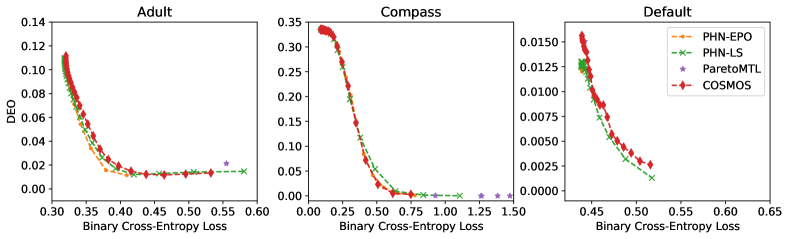
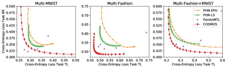
Figure 1: Comparison of the Pareto fronts on fairness and image classification datasets against SOTA baselines

5 Experimental Protocol

5.1 Research Hypotheses and Designed Experiments

We analyse our method (named COSMOS) along the following hypotheses:

• Hypothesis 1: Does our method generate qualitative Pareto fronts compared to the state-of-the-art techniques while being faster in terms of training time?
  Experiment 1: We compare our method against state of the art baselines: PHN-LS, PHN-EPO (Navon et al., 2021), ParetoMTL (Lin et al., 2019), which represent MOO baselines that are able to generate Pareto fronts with gradient-based methods. We use two sets of publicly available multi-objective datasets: in the realm of fair classification (Adult, Compass, and Default) and image classification (three variants of Multi-MNIST).

• Hypothesis 2: Does our proposed MOO approach compete strongly against single-objective baselines?
  Experiment 2: We compare our Pareto fronts against single-objective baselines on the datasets mentioned in Experiment 1.

• Hypothesis 3: Does the proposed cosine similarity penalty term achieve a wider-spread Pareto front?
  Experiment 3: We perform an ablation study on different values of $\lambda$ and $\alpha$ to understand its effect on the generated Pareto front for the image classification datasets.

• Hypothesis 4: Can our approach scale to large datasets and optimize state of the art deep neural networks?
  Experiment 4: We train EfficientNet-B4 on the larger CelebA dataset and demonstrate the quality of the achieved Pareto front as well as the training time.

5.2 Experimental Setup

The experiments aim at demonstrating the scalability as well as the quality of the results of our method. Unfortunately, these two requirements are mutually infeasible. If the state-of-the-art methods cannot scale to very deep models, then we cannot assess the comparative quality of the Pareto fronts generated by COSMOS against the prior work on the large-scale MOO setup. As a solution, we follow the strategy below:

1. We show the quality of the Pareto fronts generated by COSMOS on the identical small-scale experimental setup as in the published papers of the baselines. We clarify that all the three baselines (PHN-LS, PHN-EPO, ParetoMTL) used a toy-scaled LeNet architecture for the published experiments with small-size datasets (Multi-Mnist and Multi-Fashion).

2. After we show the quality of the Pareto fronts generated by COSMOS versus the state-of-the-art on the small-scale setup, then we demonstrate the scalability of COSMOS on the larger CelebA dataset with a deep EfficientNet model. It is important to highlight that none of the baselines can scale to this experiment. ParetoMTL needs to train one different EfficientNet network for each point on the Pareto front, while PHN-LS and PHN-EPO increase the number of trainable parameters to approximately $100\times$ that of an EfficientNet architecture.

Table 1: Results compared to the state-of-the-art methods (HV: hyper-volume, Training time in sec)

Method	Adult		Compass		Default		Multi-MNIST		Multi-Fashion		Fash.+MNIST
	HV	Time	HV	Time	HV	Time	HV	Time	HV	Time	HV	Time
Single Task	-	48	-	16	-	34	2.85	391	2.23	421	2.77	398
PHN-EPO	3.34	59	3.71	17	3.11	27	2.83	1554	2.20	1852	2.78	1715
PHN-LS	3.34	23	3.71	7	3.12	18	2.83	636	2.20	700	2.76	723
ParetoMTL	2.90	539	2.15	83	3.10	334	2.90	4087	2.24	4210	2.72	4142
COSMOS	3.34	31	3.72	17	3.12	35	2.94	501	2.32	379	2.83	498

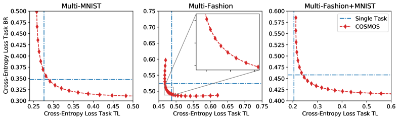
Figure 2: Comparison of COSMOS against single-objective baselines

5.3 Reproducibility

In terms of reproducibility, we set the hyperparameters for the baselines following the values defined in their papers and official implementations (details in the appendices). To make the baselines even more competitive, we perform early stopping using hyper-volume (Zitzler et al., 2007) computed on the validation set. Unless mentioned otherwise we set the batch size to 256 and use Adam  (Kingma & Ba, 2015) with a learning rate of $10^{-3}$. We report the mean scores and Pareto fronts over 5 independent runs for each method and dataset, apart from CelebA. We use (2, 2) as the reference point for hyper-volume and 25 equally distributed test rays.

Fairness on tabular data. We preprocess the data of the Adult (Dua & Graff, 2017), Compass (Angwin et al., 2016), and Default (Yeh & Lien, 2009) datasets and select “sex” as the binary sensible attribute denoted with $a$ resulting in $D_{\text{fair}}:=\{\left(x_{n},a_{n},y_{n}\right)\}^{N}_{n=1}$ with $a_{n}\in\{0,1\}$. As a differentiable fairness objective we use the hyperbolic tangent relaxation of Difference of Equality of Opportunity ($\widehat{\text{DEO}}$) (Padh et al., 2020) defined as:

$$\widehat{\text{DEO}}=\frac{1}{N}\sum_{\begin{subarray}{c}a=0\\ y=1\end{subarray}}t\left(f(\cdot);c\right)-\frac{1}{N}\sum_{\begin{subarray}{c}a=1\\ y=1\end{subarray}}t\left(f(\cdot);c\right)$$ (11)

where $t(x;c)$ denotes $\tanh\left(c\cdot\max\left(0,x\right)\right)$ and set $c=1$ for all experiments.

In compliance with the setup of prior work (Navon et al., 2021), we train a Multi-Layer Perceptron with two hidden layers (60 and 25 dimensions) and ReLU activation for 50 epochs. The binary cross-entropy and $\widehat{\text{DEO}}$ represent the multi-objective losses. Furthermore, we use 70% training, 10% validation, 20% test splits, and set $\lambda=0.01$ and $\alpha_{1}=\alpha_{2}=0.5$. Due to the high difference in scales in Default dataset we set $\alpha_{1}=0.1$, i.e. sampling more in the vertex of the cross-entropy loss.

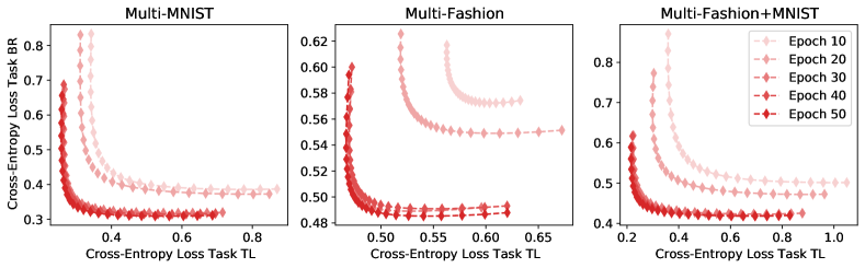
Figure 3: Convergence of the Pareto fronts generated by COSMOS on the image classification datasets

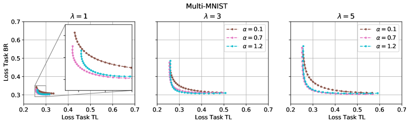
Figure 4: Ablation of the impact of the cosine similarity penalty and the Dirichlet sampling parameter on Multi-MNIST

Multi-MNIST. The Multi-MNIST datasets are constructed by overlaying two digits with a slight offset to the bottom right (BR) and top left (TL). The MTL problem is predicting the correct class for both instances at the same time. For a detailed description of the Multi-MNIST dataset and its variants see Sabour et al., 2017 and Lin et al., 2019. We use LeNet (LeCun et al., 1999) with task-specific heads similar to prior work (Sener & Koltun, 2018) and decay the learning rate at epochs 20, 40, 80, 90 by $0.1$. As losses we define cross-entropy for the BR and TL tasks. We use 10% of the training data as validation split, and set $\lambda=8$ and $\alpha_{1}=\alpha_{2}=1.2$, apart from Multi-Fashion where $\lambda=2$. For fusing the image $x$ and the preference vector $r$ we transform $r$ to the image space using transposed convolutions and then concatenate the latent vector representation with the image. Concretely, we feed $r$ to a transposed CNN with 2 layers with $J$ hidden dimensions, kernel size $4$ and $6$, and ReLU activation. This results in feature maps of size $J\times 10\times 10$ which we then upsample to $J\times 36\times 36$ and append as channels to the image. Because $J=2$, the fusion of $x$ and $r$ yields a $3\times 36\times 36$ augmented input to LeNet.

CelebA. We rescale the images of CelebA (Liu et al., 2015) to $64\times 64$ and follow the predefined splits. The deployed prediction model is an ImageNet-pretrained EfficientNet-B4 network (Tan & Le, 2019) (18m parameters) with a single-neuron output layer per objective. We set the learning rate to $5\times 10^{-4}$ and batch size to 32. Overall, the fusion of the preference vector with the image creates a $5\times 64\times 64$ input tensor. As objectives we define binary cross-entropy for two easy and two hard tasks, utilizing insights of Sener & Koltun, 2018. As hard tasks we pick “Oval Face” and “Pointy Nose” (A25 and A27), as easy tasks “Goatee” and “Mustache” (A16 and A22). The hyperparameters for COSMOS are $\lambda=3$ and $\alpha=1$; the missclassification rate is computed by taking the values from the center ray (.5, .5) although more elaborated methods are available (Wang & Rangaiah, 2017). For single task we average the individual scores, and we perform early stopping based on the validation set.

6 Results

Fairness on tabular data and Multi-MNIST.

The results of Table 1 show that COSMOS compares favorably to the baselines in terms of the quality of the Pareto front measured through the hyper-volume metric. We draw attention that COSMOS has only $5\%$ more parameters than the single-task network, whereas PHN has ca. $100$ times more parameters than the single-task network (see the appendice for details). However, due to the tiny size of the neural networks (2-layer MLP and LeNet) and the small datasets, this huge scalability gap is not reflected proportionally to the training time (a known inefficiency of GPU-based training for tiny models). Nevertheless, the empirical results indicate that COSMOS does not compromise the quality of the Pareto fronts, despite its scalability advantage, addressing Hypothesis 1.

Furthermore, COSMOS is not outperformed by the Pareto front baselines (PHN-EPO, PHN-LS and ParetoMTL) on any of the 6 datasets in terms of hyper-volume. We ommit hyper-volume for the single task baseline on the fairness datasets because unlike MTL problems, the single-task optima are mutually exclusive. Additionally, there exist trivial solutions for fairness which can achieve perfect scores, e.g. a constant classifier.

For Multi-MNIST beeing a multi-task problem, we indeed outperform the single task baseline in all three datasets, which indicates that our method fulfills Hypothesis 2. A further analysis of the Pareto fronts compared to the SOTA methods is shown in Figure 1, while a comparison to the single task method in Figure 9. Moreover, Figure 3 demonstrates that our method converges fast and is able to generate a well-spread Pareto front after 10 epochs.

Ablation study. To analyze the impact of the cosine similarity penalty, we ablate the effect of $\lambda$ and $\alpha$ on the Pareto by varying $\alpha\in(0.1,0.7,1.2)$ and $\lambda\in(1,3,5)$. Figure 10 clearly demonstrates the crucial importance of the cosine penalty and answers Hypothesis 3. In cases where $\lambda$ is small, the Pareto front is at the optimum although it is very narrow. Increasing the penalty yields a wider Pareto front. In contrast, the choice of $\alpha$ influences the quality of the Pareto front (not the width) via the sampling mechanism. For small $\alpha<1$, we sample more at the vertices of the simplex yielding high-interest points dedicated to each loss. We provide ablations on the other datasets in the appendix.

CelebA. We show the Pareto fronts for the easy and hard tasks in Figure 5. The EfficientNet model pretrained on Imagenet transfers very quickly on the Celeb-A dataset. COSMOS is capable of generating a well-spread Pareto front within a few optimization epochs and converges entirely after 25 epochs.

Table 2: Results on CelebA

	HV	Mean MCR	Time (h)
	Hard Tasks
Single Task	2.222	24.66%	3.08
COSMOS	2.221	25.29%	3.30
	Easy Tasks
Single Task	3.719	3.15%	3.11
COSMOS	3.706	3.47%	3.30

In addition, Table 2 presents the comparative analysis against the single-task baseline. COSMOS is qualitatively comparable to the baseline, but in contrast generates a full Pareto front instead of a single point. Moreover, COSMOS computes the front within a small overhead of $7\%$ additional training time when both methods run for 25 epochs. This confirms Hypothesis 4 and demonstrates that COSMOS offers a free lunch Pareto front approximation, basically at the same time budget required to train a single network on a single task.

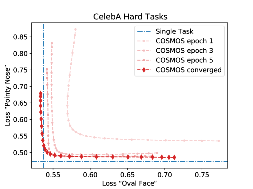
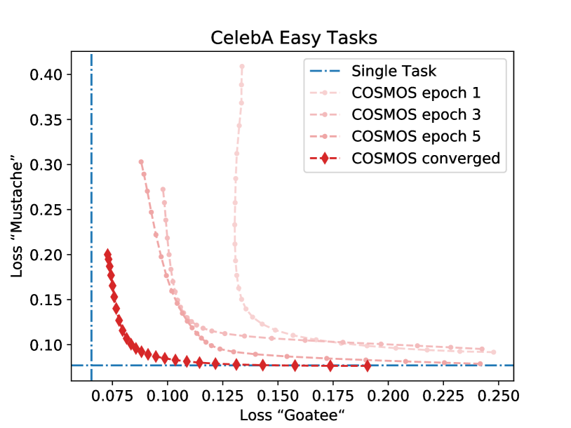
Figure 5: Pareto fronts and convergence on CelebA

7 Limitations of our method

We stress that the Pareto fronts by COSMOS are an approximation, because neural networks are not able to find the exact optimum of the linear scalarization problem. However, the provided illustrations of the approximated Pareto fronts indicate the Pareto-optimality of the achieved solutions for different preference vectors. Secondly, we highlight that conditioning the prediction network to the preference vectors cannot model objectives that do not depend on the input, e.g. an $L_{p}$ norm regularization objective on weights.

8 Conclusions

Multi-objective Optimization is a crucial task for the Machine Learning community due to the wide array of real-life tasks which are intrinsically multi-objective. Unfortunately, there exist no scalable MOO method for deep neural networks which is able to generate a Pareto front of the solutions, in a way that a practitioner can decide on the trade-offs of the competing objectives. Existing papers either relied on learning one network per solution, or deploying hyper-networks which introduce a high number of trainable parameters. In contrast, throughout this paper we introduced COSMOS, a method that is able to produce qualitative approximations of the Pareto front at a very small training time overhead compared to the single-objective optimization of one neural network. We condition the prediction model to the choice of the preference vector for the objectives and solve a regularized version of the linear scalarization problem, in a manner that a single network learns to adjust the predictions based on the inputted trade-off preference for all the objectives. Furthermore, we penalize the Pareto fronts to be widely spread by minimizing the angle between achieved solutions in the space of objectives and the inputted preference vectors. Overall, a single optimization run is required to optimize our multi-objective approach, which is asymptotically equal to the optimization of a single-objective task. In a series of experiments, we demonstrated that the approximated Pareto fronts are competitive against state-of-the-art baselines. Furthermore, we showed that COSMOS approximates a Pareto front for the CelebA dataset using the EfficientNet model with only 7% of training time overhead compared to single objective optimization tasks.

Appendix A More objectives on CelebA

Three to four objectives.

We also tried more than two objectives on CelebA using EfficientNet-B4. Here, we report the individual task errors in Table 3. As in the main paper we use the “middle ray” $\frac{1}{J}\forall j\in\{1,2,\ldots J\}$ to calculate the Missclassification Rates (MRC) for each task due to its simplicity. Please note that the MCRs do not represent the whole Pareto front but rather one particular point of it. As tasks we use “Goatee”, “Mustache”, “No Beard”, “Pale Skin” in this order. We do not report the hypervolume as obtaining evenly distributed points on a ($J-1$)-sphere is not trivial for $J>3$. We again achieve similar performance compared to the single task baseline using the same setting as in the main paper.

The Pareto front for the first three objectives is shown in Figure 6. It was obtained using 25 test rays evenly distributed on a 2-sphere using the Fibonacci sphere algorithm.

Ten random objectives.

To demonstrate that we did not cherry-pick the tasks we also evaluate COSMOS on 10 randomly picked tasks and report the MCR compared to single task. The tasks are: “Black Hair”, “Wearing Lipstick”, “Bald”, “Goatee”, “Big Nose”, “Smiling”, “Receding Hairline”, “Sideburns”, “No Beard”, “Chubby”. We report the results in Table 4. We use the same setting as in the main paper but increased the training epochs to 30.

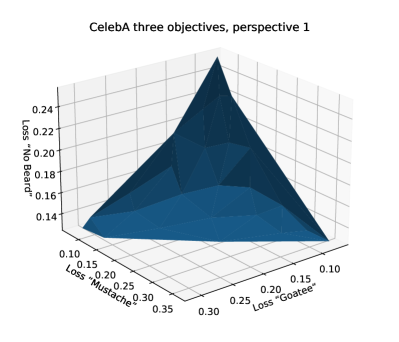
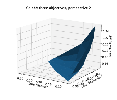
Figure 6: Pareto front found by COSMOS on CelebA with three tasks

Table 3: Results on CelebA with up to 4 objectives

	MCR Task 1	MCR Task 2	MCR Task 3	MCR Task 4
2 Tasks	3.07%	3.88%	-	-
3 Tasks	3.16%	3.93%	5.28%	-
4 Tasks	3.53%	3.59%	5.40%	3.14%
Single Task	2.87%	3.30%	4.82%	3.00%

Table 4: Results on CelebA with 10 objectives

	Single Task	Cosmos
Task 1 MCR	10.90%	11.63%
Task 2 MCR	6.55%	8.87%
Task 3 MCR	1.19%	2.00%
Task 4 MCR	2.87%	3.24%
Task 5 MCR	18.18%	18.06%
Task 6 MCR	7.52%	8.84%
Task 7 MCR	6.72%	6.87%
Task 8 MCR	2.56%	3.43%
Task 9 MCR	4.82%	6.05%
Task 10 MCR	4.59%	5.26%

Appendix B Intuition behind the Cosine Similarity penalty

We would also like to add two illustrations that demonstrate the intuition behind deploying the cosine similarity as a penalty. Figure 7 shows the difference between the Pareto front found using regular linear scalarization and what is actually desired.

Figure 8 shows how the penalty ensuring a small angle between the loss vector $\ell$ and the preference vector $\vec{r}$ pushes the solution closer towards the desired position while still minimizing both losses. This way minimizing the losses as well as reaching a position on the Pareto front are balanced during optimization.

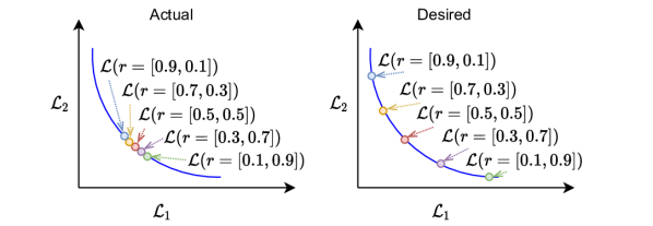
Figure 7: Pareto front found by linear scalarization (left) vs. desired (right)

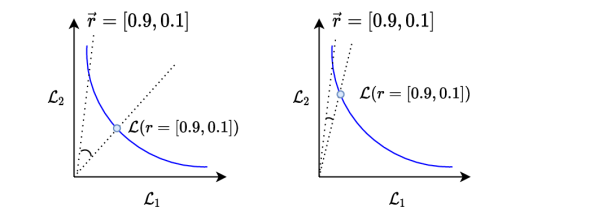
Figure 8: The effect of angle minimization on achieving a wide spread Pareto front.

Appendix C Additional figures

See Figure 9 for a comparison of COSMOS to the single task baseline for the fairness datasets.

See Figures 10 for an ablation of $\lambda$ and $\alpha$ on the datasets ommitted in the main paper. For the fairness datasets we ablate $\lambda\in\{0,0.01,0.1\}$. They demonstrate the same behaviour as for Multi-MNIST, shown in the paper, although the cosine similarity seems not as important for fairness as for the MTL tasks. This is plausible due to the large difference in scales.

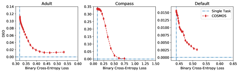
Figure 9: Comparison of COSMOS against single-objective baselines

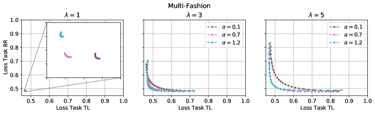
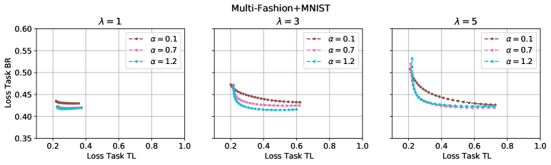
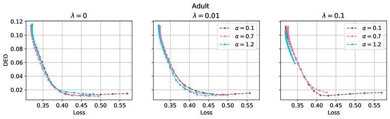
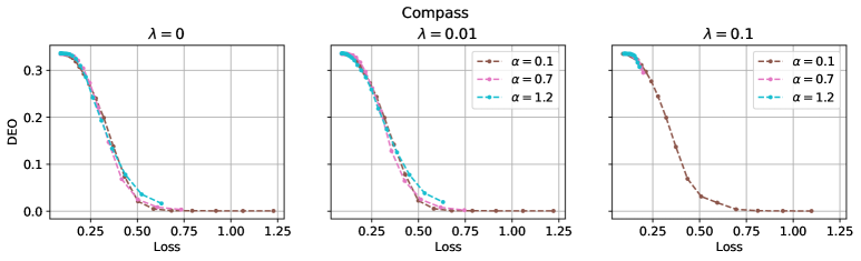
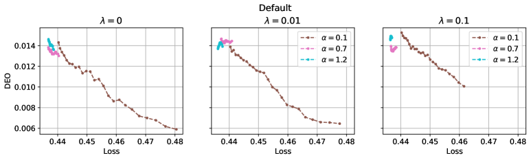
Figure 10: Ablation of the impact of the cosine similarity penalty and the Dirichlet sampling parameter.

Appendix D More detailed result tables

For more detailed results on the three fairness and image classification datasets see Table 5.

Table 5: Detailed results on fairness and image classification datasets

	Hyper Vol.	Time (Sec)	# Params.
	Adult
Single Task	3.36 $\pm$ 0.01	48	6k
PHN-EPO	3.34 $\pm$ 0.00	59	716k
PHN-LS	3.34 $\pm$ 0.00	23	716k
ParetoMTL	2.90 $\pm$ 0.05	539	6k
COSMOS	3.34 $\pm$ 0.01	31	7k
	Compass
Single Task	3.81 $\pm$ 0.00	16	2k
PHN-EPO	3.71 $\pm$ 0.01	17	304k
PHN-LS	3.71 $\pm$ 0.01	7	304k
ParetoMTL	2.15 $\pm$ 0.37	83	2k
COSMOS	3.72 $\pm$ 0.01	17	2k
	Default
Single Task	3.12 $\pm$ 0.00	34	7k
PHN-EPO	3.11 $\pm$ 0.01	27	728k
PHN-LS	3.12 $\pm$ 0.00	18	728k
ParetoMTL	3.10 $\pm$ 0.00	334	7k
COSMOS	3.12 $\pm$ 0.00	35	7k
	Multi-MNIST
Single Task	2.85 $\pm$ 0.01	391	42k
PHN-EPO	2.83 $\pm$ 0.03	1,554	3,243k
PHN-LS	2.83 $\pm$ 0.03	636	3,243k
ParetoMTL	2.90 $\pm$ 0.01	4,087	42k
COSMOS	2.94 $\pm$ 0.02	501	43k
	Multi-Fashion
Single Task	2.23 $\pm$ 0.01	421	42k
PHN-EPO	2.20 $\pm$ 0.03	1,852	3,243k
PHN-LS	2.20 $\pm$ 0.03	700	3,243k
ParetoMTL	2.24 $\pm$ 0.02	4,210	42k
COSMOS	2.32 $\pm$ 0.01	379	43k
	Multi-Fashion+MNIST
Single Task	2.77 $\pm$ 0.02	398	42k
PHN-EPO	2.78 $\pm$ 0.02	1,715	3,243k
PHN-LS	2.76 $\pm$ 0.05	723	3,243k
ParetoMTL	2.72 $\pm$ 0.02	4,142	42k
COSMOS	2.83 $\pm$ 0.03	498	43k

Appendix E Experimental Setup (further details)

We ran all experiments on a Nvidia GeForce RTX 2080 GPU with 12GB RAM. As seeds we used $1,2,3,4,42$.

Fairness on tabular data.

After preprocessing the datasets have the following dimensions: Adult $48,842\times 88$, Compass $6,172\times 20$, Default $30,000\times 90$. For HPN where we use learning rate 0.0001 set as default by the authors.

Multi-MNIST.

For ParetoMTL we decay at 15,30,45,60,75,90 it to $\gamma=0.5$ following the authors’ implementation. We train HPN for 150 epochs with learning rate 0.0001, no scheduler and $\alpha=0.2$, again following their implementation.

CelebA.

To transform the images we first resize so the smaller edge matches 64 pixels. Then we crop in the center and normalize to 0.5 mean and 0.5 standard deviation. We remove all Batchnorm layers.

References

- Angwin et al. (2016) Angwin, J., Larson, J., Mattu, S., and Kirchner, L. Machine bias, 2016.
- Chen et al. (2018) Chen, Z., Badrinarayanan, V., Lee, C.-Y., and Rabinovich, A. GradNorm: Gradient normalization for adaptive loss balancing in deep multitask networks. In Dy, J. and Krause, A. (eds.), Proceedings of the 35th International Conference on Machine Learning, volume 80 of Proceedings of Machine Learning Research, pp. 794–803, Stockholmsmässan, Stockholm Sweden, 10–15 Jul 2018. PMLR. URL http://proceedings.mlr.press/v80/chen18a.html.
- Deb et al. (2000) Deb, K., Agrawal, S., Pratap, A., and Meyarivan, T. A fast elitist non-dominated sorting genetic algorithm for multi-objective optimization: Nsga-ii. In Schoenauer, M., Deb, K., Rudolph, G., Yao, X., Lutton, E., Merelo, J. J., and Schwefel, H.-P. (eds.), Parallel Problem Solving from Nature PPSN VI, pp. 849–858, Berlin, Heidelberg, 2000. Springer Berlin Heidelberg. ISBN 978-3-540-45356-7.
- Désidéri (2012) Désidéri, J.-A. Mutiple-gradient descent algorithm for multiobjective optimization. In European Congress on Computational Methods in Applied Sciences and Engineering (ECCOMAS 2012), 2012.
- Dosovitskiy & Djolonga (2020) Dosovitskiy, A. and Djolonga, J. You only train once: Loss-conditional training of deep networks. In International Conference on Learning Representations, 2020. URL https://openreview.net/forum?id=HyxY6JHKwr.
- Dua & Graff (2017) Dua, D. and Graff, C. UCI machine learning repository, 2017. URL http://archive.ics.uci.edu/ml.
- Ehrgott (2005) Ehrgott, M. Multicriteria Optimization. Springer-Verlag, Berlin, Heidelberg, 2005. ISBN 3540213988.
- Elsken et al. (2019) Elsken, T., Metzen, J. H., and Hutter, F. Efficient multi-objective neural architecture search via lamarckian evolution. In International Conference on Learning Representations, 2019. URL https://openreview.net/forum?id=ByME42AqK7.
- Fliege & Svaiter (2000) Fliege, J. and Svaiter, B. F. Steepest descent methods for multicriteria optimization. Mathematical Methods of Operations Research, 51(3):479–494, 2000.
- Ha et al. (2016) Ha, D., Dai, A., and Le, Q. V. Hypernetworks. arXiv preprint arXiv:1609.09106, 2016.
- Kaisa (1999) Kaisa, M. Nonlinear Multiobjective Optimization, volume 12 of International Series in Operations Research & Management Science. Kluwer Academic Publishers, Boston, USA, 1999.
- Kendall et al. (2018) Kendall, A., Gal, Y., and Cipolla, R. Multi-task learning using uncertainty to weigh losses for scene geometry and semantics. In Proceedings of the IEEE conference on computer vision and pattern recognition, pp. 7482–7491, 2018.
- Kingma & Ba (2015) Kingma, D. P. and Ba, J. Adam: A method for stochastic optimization. In Bengio, Y. and LeCun, Y. (eds.), 3rd International Conference on Learning Representations, ICLR 2015, San Diego, CA, USA, May 7-9, 2015, Conference Track Proceedings, 2015. URL http://arxiv.org/abs/1412.6980.
- LeCun et al. (1999) LeCun, Y., Haffner, P., Bottou, L., and Bengio, Y. Object recognition with gradient-based learning. In Shape, contour and grouping in computer vision, pp. 319–345. Springer, 1999.
- Lin et al. (2019) Lin, X., Zhen, H.-L., Li, Z., Zhang, Q.-F., and Kwong, S. Pareto multi-task learning. In Advances in Neural Information Processing Systems, pp. 12060–12070, 2019.
- Lin et al. (2021) Lin, X., YANG, Z., Zhang, Q., and Kwong, S. Controllable pareto multi-task learning, 2021. URL https://openreview.net/forum?id=5mhViEOQxaV.
- Liu et al. (2019) Liu, S., Johns, E., and Davison, A. J. End-to-end multi-task learning with attention. In 2019 IEEE/CVF Conference on Computer Vision and Pattern Recognition (CVPR), pp. 1871–1880, 2019. doi: 10.1109/CVPR.2019.00197.
- Liu et al. (2015) Liu, Z., Luo, P., Wang, X., and Tang, X. Deep learning face attributes in the wild. In Proceedings of International Conference on Computer Vision (ICCV), December 2015.
- Ma et al. (2020) Ma, P., Du, T., and Matusik, W. Efficient continuous pareto exploration in multi-task learning. In III, H. D. and Singh, A. (eds.), Proceedings of the 37th International Conference on Machine Learning, volume 119 of Proceedings of Machine Learning Research, pp. 6522–6531. PMLR, 13–18 Jul 2020. URL http://proceedings.mlr.press/v119/ma20a.html.
- Mahapatra & Rajan (2020) Mahapatra, D. and Rajan, V. Multi-task learning with user preferences: Gradient descent with controlled ascent in pareto optimization. In International Conference on Machine Learning, pp. 6597–6607. PMLR, 2020.
- Menon & Williamson (2018) Menon, A. K. and Williamson, R. C. The cost of fairness in binary classification. In Conference on Fairness, Accountability and Transparency, pp. 107–118. PMLR, 2018.
- Navon et al. (2021) Navon, A., Shamsian, A., Chechik, G., and Fetaya, E. Learning the pareto front with hypernetworks. In International Conference on Learning Representations, 2021. URL https://openreview.net/forum?id=NjF772F4ZZR.
- Padh et al. (2020) Padh, K., Antognini, D., Glaude, E. L., Faltings, B., and Musat, C. Addressing fairness in classification with a model-agnostic multi-objective algorithm. arXiv preprint arXiv:2009.04441, 2020.
- Parisi et al. (2016) Parisi, S., Pirotta, M., and Restelli, M. Multi-objective reinforcement learning through continuous pareto manifold approximation. J. Artif. Int. Res., 57(1):187–227, September 2016. ISSN 1076-9757.
- Sabour et al. (2017) Sabour, S., Frosst, N., and Hinton, G. E. Dynamic routing between capsules. arXiv preprint arXiv:1710.09829, 2017.
- Sener & Koltun (2018) Sener, O. and Koltun, V. Multi-task learning as multi-objective optimization. In Proceedings of the 32nd International Conference on Neural Information Processing Systems, pp. 525–536, 2018.
- Standley et al. (2020) Standley, T., Zamir, A. R., Chen, D., Guibas, L., Malik, J., and Savarese, S. Which tasks should be learned together in multi-task learning? In International Conference on Machine Learning. PMLR, 2020.
- Tan & Le (2019) Tan, M. and Le, Q. EfficientNet: Rethinking model scaling for convolutional neural networks. In Chaudhuri, K. and Salakhutdinov, R. (eds.), Proceedings of the 36th International Conference on Machine Learning, volume 97 of Proceedings of Machine Learning Research, pp. 6105–6114. PMLR, 09–15 Jun 2019. URL http://proceedings.mlr.press/v97/tan19a.html.
- Valdivia et al. (2020) Valdivia, A., Sánchez-Monedero, J., and Casillas, J. How fair can we go in machine learning? assessing the boundaries of fairness in decision trees. arXiv preprint arXiv:2006.12399, 2020.
- Van Moffaert & Nowé (2014) Van Moffaert, K. and Nowé, A. Multi-objective reinforcement learning using sets of pareto dominating policies. J. Mach. Learn. Res., 15(1):3483–3512, January 2014. ISSN 1532-4435.
- Wang & Rangaiah (2017) Wang, Z. and Rangaiah, G. P. Application and analysis of methods for selecting an optimal solution from the pareto-optimal front obtained by multiobjective optimization. Industrial & Engineering Chemistry Research, 56(2):560–574, 2017.
- Yang et al. (2019) Yang, R., Sun, X., and Narasimhan, K. A generalized algorithm for multi-objective reinforcement learning and policy adaptation. In Wallach, H. M., Larochelle, H., Beygelzimer, A., d’Alché-Buc, F., Fox, E. B., and Garnett, R. (eds.), Advances in Neural Information Processing Systems 32: Annual Conference on Neural Information Processing Systems 2019, NeurIPS 2019, December 8-14, 2019, Vancouver, BC, Canada, pp. 14610–14621, 2019.
- Yeh & Lien (2009) Yeh, I.-C. and Lien, C.-h. The comparisons of data mining techniques for the predictive accuracy of probability of default of credit card clients. Expert Systems with Applications, 36(2):2473–2480, 2009.
- Zhang & Yang (2018) Zhang, Y. and Yang, Q. A survey on multi-task learning, 2018.
- Zhang et al. (2014) Zhang, Z., Luo, P., Loy, C. C., and Tang, X. Facial landmark detection by deep multi-task learning. In Fleet, D., Pajdla, T., Schiele, B., and Tuytelaars, T. (eds.), Computer Vision – ECCV 2014, pp. 94–108, Cham, 2014. Springer International Publishing. ISBN 978-3-319-10599-4.
- Zitzler et al. (2007) Zitzler, E., Brockhoff, D., and Thiele, L. The hypervolume indicator revisited: On the design of pareto-compliant indicators via weighted integration. In International Conference on Evolutionary Multi-Criterion Optimization, pp. 862–876. Springer, 2007.