One-point statistics for turbulent pipe flow
up to $\Rey_{\tau}\approx 6000$

Abstract

We study turbulent flows in a smooth straight pipe of circular cross–section up to $\Rey_{\tau}\approx 6000$ using direct–numerical-simulation (DNS) of the Navier–Stokes equations. The DNS results highlight systematic deviations from Prandtl friction law, amounting to about $2\%$, which would extrapolate to about $4\%$ at extreme Reynolds numbers. Data fitting of the DNS friction coefficient yields an estimated von Kármán constant $k\approx 0.387$, which nicely fits the mean velocity profile, and which supports universality of canonical wall-bounded flows. The same constant also applies to the pipe centerline velocity, thus providing support for the claim that the asymptotic state of pipe flow at extreme Reynolds numbers should be plug flow. At the Reynolds numbers under scrutiny, no evidence for saturation of the logarithmic growth of the inner peak of the axial velocity variance is found. Although no outer peak of the velocity variance directly emerges in our DNS, we provide strong evidence that it should appear at $\Rey_{\tau}\gtrsim 10^{4}$, as a result of turbulence production exceeding dissipation over a large part of the outer wall layer, thus invalidating the classical equilibrium hypothesis.

1 Introduction

Turbulent flow in circular pipes has always attracted the interest of scientists, owing to its prominent importance in the engineering practice and because of the beautiful simplicity of the setup. In this respect, the pioneering flow visualizations of Reynolds (1883) may be regarded as a milestone for the understanding of turbulent and transitional flows. The most extensive experimental measurements of high-Reynolds-number pipe flows have been carried out in modern times in the Princeton Superpipe pressurized facility (Zagarola & Smits, 1998; McKeon et al., 2005; Hultmark et al., 2010). Those investigations have allowed scientists to measure the main flow features as friction and mean velocity profiles with high precision, and they currently constitute the most comprehensive database for the study of pipe turbulence. However, even the use of specialized micro-fabricated hot-wire probes could not provide fully reliable information about the viscous and buffer layers at high Reynolds numbers (Hultmark et al., 2012). Additional experimental studies of pipe turbulence have been carried out in the high-Reynolds-number actual flow facility (Hi-Reff), a water tunnel with relatively large diameter, which allows for accurate estimation of friction (Furuichi et al., 2015, 2018). Recently, the CICLoPE facility of the University of Bologna (Fiorini, 2017; Willert et al., 2017) has been set up, whose large diameter (about 1m) offers a well-established turbulent flow with relatively large viscous scales, thus granting higher spatial resolution. Flows in different facilities seem to have sensibly different properties in terms of friction and mean velocity profiles, which we will comment on.

Numerical simulation of pipe turbulence flow has received less interest than other canonical flows, the plane channel in particular, because of additional difficulties involved with discrete solution of the Navier–Stokes equations in cylindrical coordinates, with special reference to treatment of the geometrical singularity at the pipe axis. Early numerical simulations of turbulent pipe flow were carried out by Eggels et al. (1994), at friction Reynolds number $\Rey_{\tau}=180$ ($\Rey_{\tau}=u_{\tau}R/\nu$, with $u_{\tau}=(\tau_{w}/\rho)^{1/2}$ the friction velocity, $R$ the pipe radius, and $\nu$ the fluid kinematic viscosity). Effects of drag reduction associated with pipe rotation were later studied by Orlandi & Fatica (1997). Higher Reynolds numbers (up to $\Rey_{\tau}\approx 1140$) were reached by Wu & Moin (2008), which first allowed to observe a near logarithmic layer in the mean velocity profile. Flow visualizations and two-point correlation statistics pointed to the existence of high-speed wavy structures in the pipe core region which are elongated in the axial direction, and whose streamwise and azimuthal dimensions do not change substantially with the Reynolds number, when normalized in outer units. Further follow-up DNS studies have been carried out by El Khoury et al. (2013); Chin et al. (2014); Ahn et al. (2013). At present, the highest Reynolds number in pipe flow ($\Rey_{\tau}\approx 3000$) has been reached in the study of Ahn et al. (2015). Although no sizeable logarithmic layer is present yet at those conditions, some effects associated with significant scale separation between inner- and outer-scale turbulence were observed, as the presence of a $k^{-1}$ ($k$ being the wavenumber in any wall-parallel direction) power-law ranges in the velocity spectra.

Despite inherent limitations in the Reynolds numbers which can be attained, DNS has the advantage over experiments of yielding immediate access to the near-wall region, and of allowing scientists to measure some flow properties, e.g. the turbulence dissipation rate, which can hardly be measured in experiments. Hence, it is generally claimed that DNS data at increasing Reynolds numbers are needed to prove or disprove theoretical claims related to departure (or not) of the statistical properties of wall-bounded turbulence from the universal wall scaling (Cantwell, 2019; Monkewitz, 2021; Chen & Sreenivasan, 2021). In this paper we thus present DNS data of turbulent flow in a smooth circular pipe at $\Rey_{\tau}\approx 6000$, which is two times higher that the previous state of art. Relying on the DNS data, we revisit current theoretical inferences and discuss implications about possible trends in the extreme Reynolds number regime.

2 The numerical dataset

The code used for DNS is the spin-off of an existing solver previously used to study Rayleigh-Bénard convection in cylindrical containers at extreme Rayleigh numbers (Stevens et al., 2013). That code is in turn the evolution of the solver originally developed by Verzicco & Orlandi (1996), and used for DNS of pipe flow by Orlandi & Fatica (1997). A second-order finite-difference discretization of the incompressible Navier-Stokes equations in cylindrical coordinates is used, based on the classical marker-and-cell method (Harlow & Welch, 1965), with staggered arrangement of the flow variables to remove odd-even decoupling phenomena and guarantee discrete conservation of the total kinetic energy in the inviscid flow limit. Uniform volumetric forcing is applied to the axial momentum equation to maintain constant mass flow rate in time. The Poisson equation resulting from enforcement of the divergence-free condition is efficiently solved by double trigonometric expansion in the periodic axial and azimuthal directions, and inversion of tridiagonal matrices in the radial direction (Kim & Moin, 1985). An extensive series of previous studies about wall-bounded flows from this group proved that second-order finite-difference discretization yields in practical cases of wall-bounded turbulence results which are by no means inferior in quality to those of pseudo-spectral methods (e.g. Pirozzoli et al., 2016; Moin & Verzicco, 2016). A crucial issue is the proper treatment of the polar singularity at the pipe axis. A detailed description of the subject is reported in Verzicco & Orlandi (1996), but basically, the radial velocity $u_{r}$ in the governing equations is replaced by $q_{r}=ru_{r}$ ($r$ is the radial space coordinate), which by construction vanishes at the axis. The governing equations are advanced in time by means of a hybrid third-order low-storage Runge-Kutta algorithm, whereby the diffusive terms are handled implicitly, and convective terms in the axial and radial direction explicitly. An important issue in this respect is the convective time step limitation in the azimuthal direction, due to intrinsic shrinking of the cells size toward the pipe axis. To alleviate this limitation we rely on implicit treatment of the convective terms in the azimuthal direction (Akselvoll & Moin, 1996; Wu & Moin, 2008), which enables marching in time with similar time step as in planar domains flow in practical computations. In order to minimize numerical errors associated with implicit time stepping, in the present code explicit and explicit discretizations of the azimuthal convective terms are linearly blended with the radial coordinate, in such a way that near the pipe wall the treatment is fully explicit, and near the pipe axis it is fully implicit. The code was adapted to run on clusters of graphic accelerators (GPUs), using a combination of CUDA Fortran and OpenACC directives, and relying on the CUFFT libraries for efficient execution of FFTs (Ruetsch & Fatica, 2014). The DNS were carried out on the Marconi-100 machine based at CINECA (Italy), relying on NVIDIA Volta V100 graphic cards. Specifically, 1024 GPUs were used for DNS-F.

Dataset	$L_{z}/R$	Mesh ($N_{\theta}\times N_{r}\times N_{z}$)	$\Rey_{b}$	$\lambda$	$\Rey_{\tau}$	$T/\tau_{t}$	Line style
DNS-A	15	$256\times 67\times 256$	$5300$	$0.03700$	$180.3$	204.0
DNS-B	15	$768\times 140\times 768$	$17000$	$0.02716$	$495.3$	87.4
DNS-C	15	$1792\times 270\times 1792$	$44000$	$0.02136$	$1136.6$	25.9
DNS-C-SH	7.5	$1792\times 270\times 986$	$44000$	$0.02164$	$1144.2$	31.1	NA
DNS-C-LO	30	$1792\times 270\times 3944$	$44000$	$0.02128$	$1134.6$	24.5	NA
DNS-C-FT	15	$3944\times 270\times 1792$	$44000$	$0.02114$	$1131.0$	31.3	NA
DNS-C-FR	15	$1792\times 540\times 1792$	$44000$	$0.02132$	$1135.7$	28.6	NA
DNS-C-FZ	15	$1792\times 270\times 3944$	$44000$	$0.02132$	$1135.7$	15.5	NA
DNS-D	15	$3072\times 399\times 3072$	$82500$	$0.01836$	$1976.0$	22.4
DNS-E	15	$4608\times 540\times 4608$	$133000$	$0.01659$	$3028.1$	16.6
DNS-F	15	$9216\times 910\times 9216$	$285000$	$0.01428$	$6019.4$	8.32

Table 1: Flow parameters for DNS of pipe flow. $R$ is the pipe radius, $L_{z}$ is the pipe axial length, $N_{\theta}$, $N_{r}$ and $N_{z}$ are the number of grid points in the azimuthal, radial and axial directions, respectively, $\Rey_{b}=2Ru_{b}/\nu$ is the bulk Reynolds number, $\lambda=8\tau_{w}/(\rho u_{b}^{2})$ is the friction factor, $\Rey_{\tau}=u_{\tau}R/\nu$ is the friction Reynolds number, $T$ is the time interval used to collect the flow statistics, and $\tau_{t}=R/u_{\tau}$ is the eddy turnover time.

Dataset	$\lambda$	$U_{{}_{CL}}^{+}$	$<u_{z}^{2}>^{+}_{{}_{IP}}$	$y^{+}_{{}_{IP}}$	$\epsilon^{+}_{{}_{11w}}$
DNS-A	$0.03700\pm 0.15\%$	$19.30\pm 0.087\%$	$7.129\pm 0.26\%$	$14.95\pm 0.24\%$	$0.1168\pm 0.47\%$
DNS-B	$0.02716\pm 0.074\%$	$21.81\pm 0.17\%$	$7.352\pm 0.17\%$	$14.28\pm 0.010\%$	$0.1506\pm 0.21\%$
DNS-C	$0.02136\pm 0.13\%$	$24.07\pm 0.18\%$	$7.995\pm 0.29\%$	$14.66\pm 0.073\%$	$0.1697\pm 0.37\%$
DNS-C-SH	$0.02164\pm 0.14\%$	$24.09\pm 0.20\%$	$8.071\pm 0.44\%$	$14.37\pm 0.11\%$	$0.1952\pm 0.54\%$
DNS-C-LO	$0.02128\pm 0.16\%$	$24.17\pm 0.11\%$	$7.965\pm 0.29\%$	$14.62\pm 0.058\%$	$0.1704\pm 0.40\%$
DNS-C-FT	$0.02114\pm 0.12\%$	$24.28\pm 0.14\%$	$7.948\pm 0.27\%$	$14.66\pm 0.078\%$	$0.1691\pm 0.34\%$
DNS-C-FR	$0.02132\pm 0.25\%$	$24.10\pm 0.12\%$	$7.886\pm 0.31\%$	$14.41\pm 0.096\%$	$0.1741\pm 0.60\%$
DNS-C-FZ	$0.02132\pm 0.21\%$	$24.07\pm 0.26\%$	$8.168\pm 0.38\%$	$14.89\pm 0.14\%$	$0.1727\pm 0.44\%$
DNS-D	$0.01839\pm 0.25\%$	$25.56\pm 0.34\%$	$8.397\pm 0.43\%$	$14.79\pm 0.098\%$	$0.1822\pm 0.57\%$
DNS-E	$0.01658\pm 0.26\%$	$26.47\pm 0.27\%$	$8.681\pm 0.69\%$	$14.87\pm 0.13\%$	$0.1903\pm 0.93\%$
DNS-F	$0.01428\pm 0.36\%$	$28.05\pm 0.35\%$	$9.108\pm 0.72\%$	$15.14\pm 0.20\%$	$0.1993\pm 1.10\%$

Table 2: Uncertainty estimation study: mean values of representative quantities and standard deviation of their estimates. $\lambda$ is the friction factor, $U_{{}_{CL}}^{+}$ is the mean pipe centerline velocity, $<u_{z}^{2}>^{+}_{{}_{IP}}$ is the peak axial velocity variance and $y^{+}_{{}_{IP}}$ is its distance from the wall, and $\epsilon^{+}_{{}_{11w}}$ is the dissipation rate of $<u_{z}^{2}>$ at the wall.

Source	Type	$\Rey_{\tau}$ range	Symbols
Wu & Moin (2008)	DNS	180, 1140	$\blacksquare$
El Khoury et al. (2013)	DNS	180-1000
Chin et al. (2014)	DNS	180-2000	$\blacktriangle$
Ahn et al. (2013), Ahn et al. (2015)	DNS	180-3000
Durst et al. (1995)	EXP	250
Swanson et al. (2002)	EXP	170-1500
Fiorini (2017)	EXP	3000-35000
Willert et al. (2017)	EXP	5400-40000
Nagib et al. (2017)	EXP	8000-40000
McKeon et al. (2005)	EXP	1800-32900
Hultmark et al. (2012)	EXP	2000-20000
Furuichi et al. (2015), Furuichi et al. (2018)	EXP	200-53000	$\bigtriangledown$
Schultz & Flack (2013)	EXP (channel)	1000-6000
Lee & Moser (2015)	DNS (channel)	180-5200

Table 3: List of other references for data used in the paper

Numerical simulations are carried out with periodic boundary conditions in the axial ($z$) and azimuthal ($\theta$) directions. The velocity field is then controlled by two parameters, namely the bulk Reynolds number ($\Rey_{b}=2Ru_{b}/\nu$, with $R$ the pipe radius, $u_{b}$ the fluid bulk velocity, and $\nu$ its kinematic viscosity), and the relative pipe length, $L_{z}/R$. A list of the main simulations that we have carried out is given in table 1. The mesh resolution is designed based on well-established criteria in the wall turbulence community. In particular, the collocation points are distributed in the wall-normal direction so that about thirty points are placed within $y^{+}\leq 40$ ($y=R-r$ is the wall distance, and the + superscript is used to denote normalization with respect to $u_{\tau}$ and $\nu$), with the first grid point at $y^{+}\approx 0.05$. The mesh is progressively stretched in the outer wall layer in such a way that the mesh spacing is proportional to the local Kolmogorov length scale, which there varies as $\eta^{+}\approx 0.8\,{y^{+}}^{1/4}$ (Jiménez, 2018), and the radial spacing at the pipe axis is $\Delta y^{+}\approx 8.8$. Additional details are provided in a specifically focused publication (Pirozzoli & Orlandi, 2021). Regarding the axial and azimuthal directions, finite-difference simulations of wall-bounded flows yield grid-independent results as long as $\Delta x^{+}\approx 10$, $R^{+}\Delta\theta\approx 4.5$ (Pirozzoli et al., 2016), hence the associated number of grid points scales as $N_{z}\approx L_{z}/R\times\Rey_{\tau}/10$, $N_{\theta}\sim 2\pi\times\Rey_{\tau}/4.5$. All DNS have been carried out at CFL number close to unity, based on the radial convective time step limitation. The CFL number along the axial direction is typically smaller by a factor two. The time step expressed in wall units ($\nu/u_{\tau}^{2}$) ranges from $\Delta t^{+}=0.55$ in DNS-A to $\Delta t^{+}=0.15$ in DNS-F. According to the established practice (Hoyas & Jiménez, 2006; Lee & Moser, 2015; Ahn et al., 2015), the time intervals used to collect the flow statistics are reported in terms of eddy-turnover times, $\tau_{t}=R/u_{\tau}$. For reference, the time window used to collect the flow statistics in DNS-F amounts to about 13.1 flow-through times ($L_{z}/u_{b}$ time units).

The sampling errors for some key properties discussed in this paper have been estimated using the method of Russo & Luchini (2017), based on extension of the classical batch means approach. The results of the uncertainty estimation analysis are listed in table 2, where we provide expected values and associated standard deviation for the friction factor ($f$), mean centerline velocity ($U_{{}_{CL}}$), peak axial velocity variance and its position ($\left<{u_{z}^{2}}\right>_{{}_{IP}}$ and $y_{{}_{IP}}$, respectively), and dissipation rate of streamwise velocity variance ($\epsilon_{{}_{11w}}$). Here and elsewhere, capital letters are used to denote flow properties averaged in the homogeneous spatial directions and in time, brackets denote the averaging operator, and lower-case letters to denote fluctuations from the mean. We find that the sampling error is generally quite limited, being larger in the largest DNS, which have been run for shorter time. In particular, in DNS-F the expected sampling error in friction, centerline velocity and peak velocity variance is about $0.5\%$, whereas it is about $1\%$ for the wall dissipation. Additional tests aimed at establishing the effect of axial domain length and grid size have been carried out for the DNS-C flow case, whose results are also reported in table 2. We find that doubling the pipe length yields a change in the basic flow properties of about $0.2-0.3\%$, whereas halving it yields changes of about $1\%$ in friction and peak velocity variance, and up to $10\%$ in the wall dissipation. Hence, consistent with previous studies (Chin et al., 2010), we believe that the selected pipe length ($L_{z}/R=15$) is representative of an infinitely long pipe, at least for the purposes of the present study. In order to quantify uncertainties associated with numerical discretization, additional simulations have been carried out by doubling the grid points in the azimuthal, radial and axial directions, respectively. Based on the data reported in the table, after discarding the short pipe case, we can thus quantify the uncertainty due to numerical discretization and limited pipe length to be about $0.3\%$ for the friction coefficient and pipe centerline velocity, $0.6\%$ for the peak velocity variance, and $0.9\%$ for the wall dissipation.

3 Results

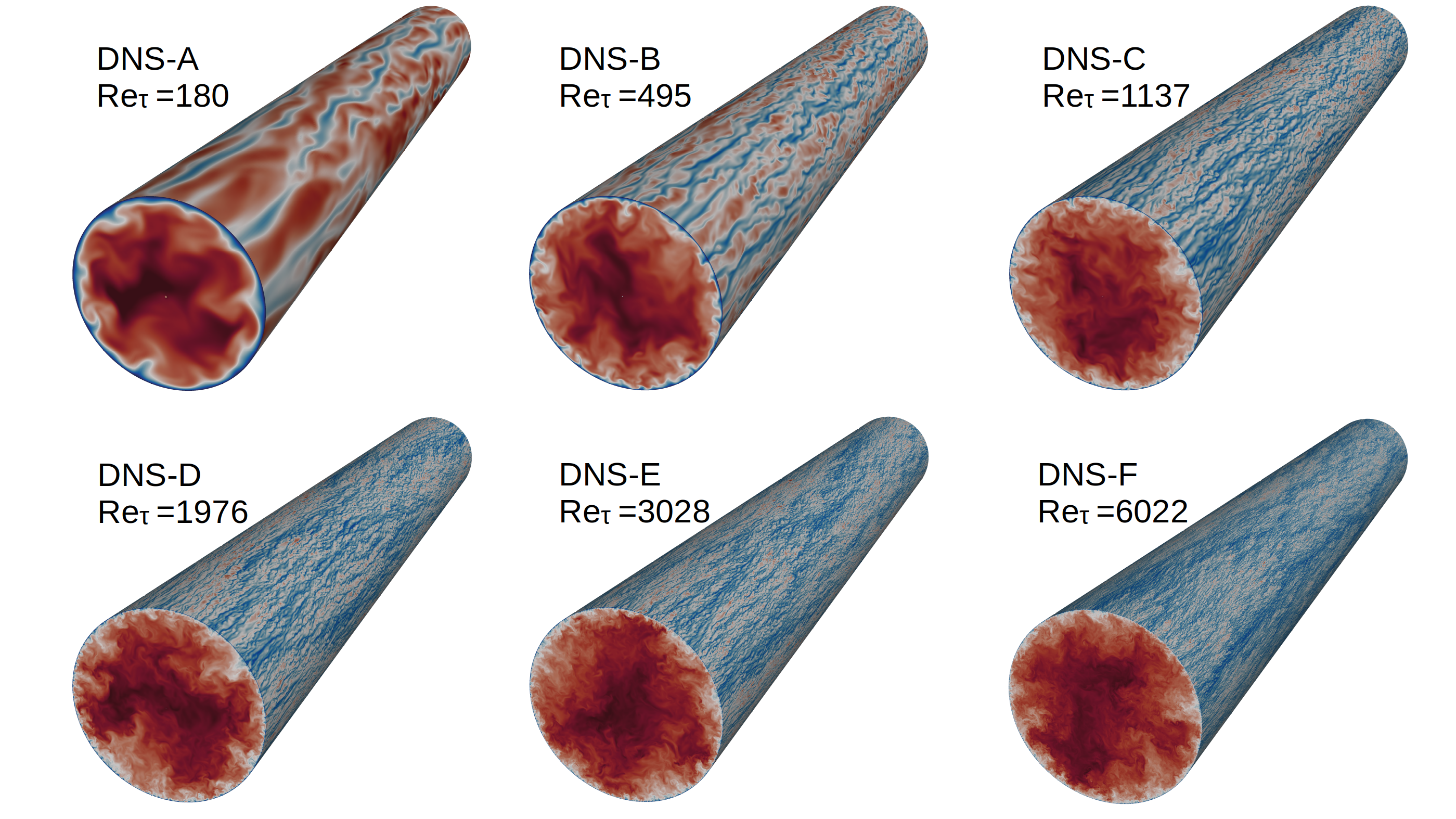
Figure 1: Instantaneous streamwise velocity contours (colour scale from blue to red) in turbulent pipe flow as obtained from DNS. Contours are shown on a cross-stream plane and on a near-wall cylindrical shell ($y^{+}\approx 15$).

Qualitative information about the structure of the flow field is provided by instantaneous perspective views of the axial velocity field, provided in figure 1. Although finer-scale details are visible at the higher $\Rey$, the flow in the cross-stream planes is always characterized by a limited number of bulges distributed along the azimuthal direction, which closely recall the POD modes identified by Hellström & Smits (2014), and which correspond to alternating intrusions of high-speed fluid from the pipe core and ejections of low-speed fluid from the wall. Streaks are visible in the near-wall cylindrical shells, whose organization has clear association with the cross-stream pattern. Specifically, regardless of the Reynolds number, $R$-sized low-streaks are observed in association with large-scale ejections, whereas $R$-sized high-speed streaks occur in the presence of large-scale inrush from the core flow. At the same time, smaller streaks scaling in wall units appear, corresponding to buffer-layer ejections/sweeps. Hence, organization of the flow on at least two length scales is apparent here, whose separation increases with $\Rey_{\tau}$.

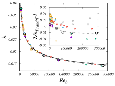
(a)  (b) 

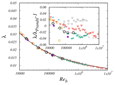
Figure 2: Friction factor as a function of bulk Reynolds number, in linear (a) and in semi-logarithmic (b) scale. Circles denote present DNS data, other symbols are defined in table 3. The solid line corresponds to the classical Prandtl friction law as given in equation (2), whereas the dashed grey line corresponds to a fit of the DNS data. Relative deviations with respect to the Prandtl friction law are shown in the insets.

Mean friction is obviously a parameter of paramount importance as it is related to power expenditure to sustain the flow. In figure 2, we show the friction factor, namely

$$\lambda=\frac{8\tau_{w}}{\rho u_{b}^{2}}.$$ (1)

A correlation generally used for smooth pipes is the Prandtl friction law,

$$1/{\lambda}^{1/2}=A\log_{10}(\Rey_{b}{\lambda}^{1/2})-B,$$ (2)

where $A=\log 10/(2k\sqrt{2})$, with $k$ the von Kármán log-law constant. The standard values $A=2.0$, $B=0.8$, were derived by fitting the experimental data of Nikuradse (1933). Reynolds-number-dependent corrections to the standard friction law were introduced by McKeon et al. (2005) in order to improve the fitting of Superpipe data. Figure 2 shows overall agreement of all DNS and experimental data with Prandtl law. However, closer scrutiny (see the figure insets) highlights some scatter. Regarding DNS, all datasets overshoot Prandtl law at low Reynolds number, although to a quite different extent. In fact, the data of Wu & Moin (2008), El Khoury et al. (2013), Chin et al. (2014) exceed the theoretical values by up to $4\%$, whereas our data tend to be much more consistent with those of Ahn et al. (2015). We believe that this difference may be related to different grid resolution in the azimuthal direction, which was $R^{+}\Delta\theta=7-8$ in those previous studies, and $4-5$ in our DNS. Our data in fact show minimal overshoot at low Reynolds number, and consistent undershoot from Prandtl law by about $2\%$. Regarding experiments, Superpipe data typically tend to lie above the theoretical curve by about $2\%$, whereas the CICLoPE and Hi-Reff data tend to fall short of it. Although the range of data overlap is not extensive, it appears that DNS data tend to be more consistent with the CICLoPE and Hi-Reff data than with other datasets. Fitting the current DNS data with a functional relationship as (2), yields $A\approx 2.102$, $B\approx 1.148$, with an inferred value of the von Kármán constant of $k=0.387\pm 0.004$, with uncertainty estimates based on $95\%$ confidence bounds from the curve-fitting procedure. This value is extremely close to that suggested by Furuichi et al. (2018), who reported $k=0.386$ as an average value over a very wide range of Reynolds numbers, and also very close to values reported in boundary layers (Nagib & Chauhan, 2009) and channels (Lee & Moser, 2015). If this trend is extrapolated, deviations of about $4\%$ from the standard Prandtl law would result at $\Rey_{b}=10^{7}$.

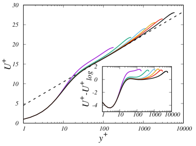
(a)  (b) 

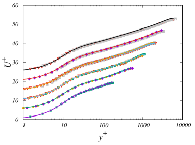
Figure 3: Inner-scaled mean velocity profiles obtained with our DNS (a), and compared with previous DNS and experiments (b). Deviations from the assumed logarithmic wall law, $U_{log}^{+}=\log y^{+}/0.387+4.53$, are highlighted in the inset of panel (a). For greater clarity, profiles in panel (b) are offset in the vertical direction by five wall units steps. Lines denote present DNS data, with color code as in table 1, and symbols denote data from other authors, as in table 3.

The mean velocity profile in turbulent pipes has received extensive attention from theoretical studies, much of the early debate being focused on whether a log law or a power law better fits the experimental results (Barenblatt et al., 1997), mainly carried out in the Superpipe facility (Zagarola & Smits, 1998; McKeon et al., 2005). Recent studies have highlighted the need for corrections to the baseline log law in order to accurately describe the velocity profile throughout the log layer into the core part of the flow (Luchini, 2017; Cantwell, 2019; Monkewitz, 2021). In figure 3, we show the series of velocity profiles computed with the present DNS, compared with previous DNS and experimental data. Overall, good agreement is observed across various sources as far as the inner and the overlap regions are concerned, with data gradually approaching a logarithmic distribution, here identified by visual fitting as $U^{+}=1/k\log y^{+}+4.53$, using the value of $k=0.387$ determined from friction data. This is quite close to estimates based on direct fitting of the mean velocity profile in pipe flow (Marusic et al., 2013), which yielded $U^{+}=1/0.391\log y^{+}+4.34$. The DNS velocity profiles for $\Rey_{\tau}\geq 10^{3}$ follow this distribution with deviations of no more than $0.1$ wall units from $y^{+}\approx 30$ to $y/R\approx 0.15$, whence the core region develops. Differences with respect to previous DNSs are concentrated in the core region, which seemingly stronger wake in some datasets, including our own, Wu & Moin (2008) and Ahn et al. (2013), and weaker in others (El Khoury et al., 2013; Chin et al., 2014), reflecting previously noted differences in the friction coefficient. Especially satisfactory is the excellent agreement between our DNS-E velocity profile and the data of Ahn et al. (2015) at $\Rey_{\tau}\approx 3000$. Comparison of our DNS dataset with experimental data also shows overall good agreement, although some differences are quite clear in the core region, in which Superpipe experiments consistently yield lower $U^{+}$, which translates into lower friction.

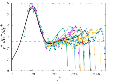
(a)  (b) 

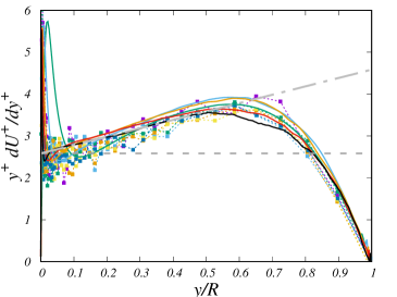
Figure 4: Log-law diagnostic function as defined in equation (3), expressed as a function of inner-scaled (a) and outer-scaled (b) wall distance. The dashed horizontal line denotes the inverse Kármán constant, $1/0.387$, and the dash-dotted lines in panel (b) denotes the linear fit (4), with $k=0.387$, $\alpha=2.0$, $\beta=0$. Lines denote present DNS data, with color code as in table 1, and symbols denote Superpipe data (McKeon et al., 2005) at $\Rey_{\tau}=1825,3328,6617,10914,19119,32870$.

More refined information on the behaviour of the mean velocity profile can be gained from inspection of the log-law diagnostic function

$$\Xi=y^{+}\,\mathrm{d}{U}^{+}/\mathrm{d}y^{+},$$ (3)

which is shown in figure 4, and whose constancy would imply the presence of a genuine logarithmic layer in the mean velocity profile. The figure supports universality of the inner-scaled axial velocity for $\Rey_{\tau}\gtrsim 10^{3}$, up to $y^{+}\approx 100$, where $\Xi$ attains a minimum, and the presence of an outer maximum at $y/R\approx 0.6$. Between these two sites the distribution is roughly linear, as can be better appreciated in panel (b), with nearly constant slope when expressed in outer coordinates. Approximate linear variation of the diagnostic function in channel flow was observed by Jiménez & Moser (2007), who, based on refined overlap arguments expressed by Afzal & Yajnik (1973), proposed the following fit

$$\Xi=\frac{1}{k}+\frac{\beta}{\Rey_{\tau}}+\alpha\frac{y}{R},$$ (4)

where $\alpha$, $\beta$ are adjustable constants, and $k$ is the von Kármán constant. Here we find that the set of constants $k=0.387$, $\alpha=2.0$, $\beta=0$, yields overall good approximation of the pipe DNS data. The consequence is that a genuine logarithmic layer would only be attained at infinite Reynolds number. In this respect, Superpipe data seem to suggest the formation of a plateau at $\Rey_{\tau}\gtrsim 10^{4}$, although the scatter of points is quite significant. Hence, DNS at higher Reynolds number would be most welcome to confirm or refute our findings, and possibly determine more accurate values of the extended log-law constants in (4).

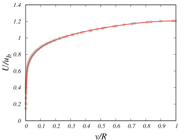
(a)  (b) 

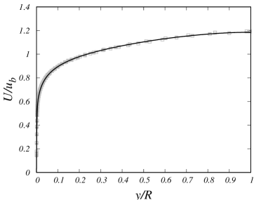
Figure 5: Mean velocity profiles in outer scaling. Data of flow case DNS-E (left) are compared with Superpipe data at $\Rey_{\tau}=3328$ and $\Rey_{\tau}=3334$, and data of flow case DNS-F (right) with Superpipe data at $\Rey_{\tau}=5411$ and $\Rey_{\tau}=6617$.

Comparison with Superpipe data is presented in outer units in figure 5, limited to the higher $\Rey_{\tau}$ cases. Despite differences in the Reynolds number, the velocity profiles now agree very well, throughout the outer layer. This observation would suggest problems with correct estimation of the friction velocity, which however seems unlikely both in DNS, in which we independently evaluate friction velocity by computing the wall derivative of the velocity profile and from momentum balance, and in experiments, as measurements of the pressure drop are regarded to have low uncertainty. Hence, reasons for this discrepancy are not known, and additional experiments as those currently carried out in the large CICLoPE facility would be especially useful and welcome. Unfortunately, velocity profiles along the full radial span are not available at the moment for that facility.

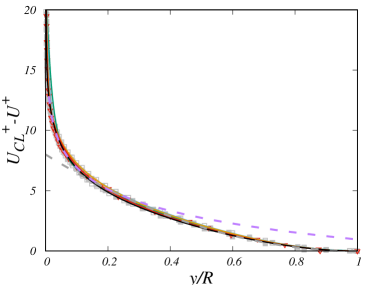
(a)  (b) 

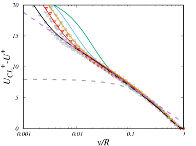
Figure 6: Defect velocity profiles for DNS and experiments, in linear (a) and semi-logarithmic (b) scale. The dashed grey line marks a parabolic fit of the DNS data ($U^{+}_{{}_{CL}}-U^{+}=8.0(1-y/R)^{2}$), and the dashed purple line the outer-layer logarithmic fit $U^{+}_{{}_{CL}}-U^{+}=0.961-1/0.387\log(y/R)$.

The structure of the core region is examined in detail in figure 6, where the mean velocity profiles are shown in defect form. Although full outer-layer similarity is not reached at the conditions of our DNS study (also see the inset of figure 3(a)), scatter across the Reynolds number range and with respect to Superpipe profiles for $y/R\geq 0.2$ is no larger than $5\%$. As suggested by Pirozzoli (2014), the core velocity profiles can be closely approximated with a simple quadratic function, reflecting near constancy of the eddy viscosity. In particular, we find that the formula

$$U_{{}_{CL}}^{+}-U^{+}=C_{{}_{O}}\left(1-y/R\right)^{2},$$ (5)

fits the DNS data with $C_{{}_{O}}=8.0$ well, and it smoothly connects at $y/R\approx 0.2$ with the logarithmic profile expressed in outer form,

$$U_{{}_{CL}}^{+}-U^{+}=-\frac{1}{k}\,\log(y/R)+B,$$ (6)

where again $k=0.387$, and data fitting yields $B=0.961$. While of course better descriptions of the core velocity profiles are possible based on more elaborate functional relationships (Luchini, 2017), the composite profile matching equations (5) and (6) yields a reasonable representation of the whole outer-layer mean velocity profile within the scatter of available data.

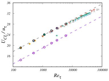
(a)  (b) 

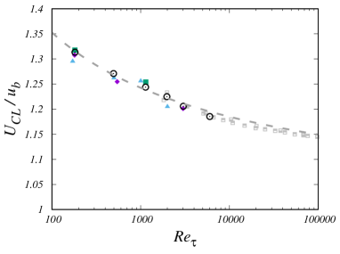
Figure 7: Mean pipe centerline velocity ($U_{{}_{CL}}$) expressed in inner (a) and in outer (b) units. The dashed grey line corresponds to a fit of the DNS data. DNS data are shown as circle symbols, and the corresponding logarithmic fits are shown as thick dashed lines. Purple lines and symbols are used for the bulk velocity, $u_{b}$. For the nomenclature of other symbols, refer to table 3.

Finer evaluation of similarities and differences between DNS and experiments is provided in figure 7, where we show the mean centerline velocity, $U_{{}_{CL}}$, normalized by the friction velocity (left panel), and by the bulk velocity (right panel), as a function of the friction Reynolds number. Consistently with theoretical expectations (e.g. Monkewitz, 2021), data suggest logarithmic increase with $\Rey_{\tau}$ according to

$$U_{{}_{CL}}^{+}=\frac{1}{k_{{}_{CL}}}\log\Rey_{\tau}+B_{{}_{CL}},$$ (7)

where we find $k_{{}_{CL}}=k=0.387$ as for the friction law, and $B_{{}_{CL}}=5.85$. For convenience, the trend of $u_{b}/u_{\tau}$ is also presented, having in fact the same logarithmic growth with $\Rey_{\tau}$. With some previously noted differences, all pipe flow DNSs seem to exhibit a consistent trend in the accessible range. While the trend is very similar at low Reynolds number, experimental data yield consistently lower values of $U_{{}_{CL}}^{+}$, especially those from the Superpipe. At Reynolds numbers higher than about $\Rey_{\tau}=10^{4}$, experiments seem to suggest milder growth rate, although significant differences emerge between the Superpipe and the Hi-Reff datasets. Hence, whether this is the result of a change of behaviour at high Reynolds number, or some form of shortcoming of experiments is difficult to say. As a result of the observed identity (or very close vicinity) of the von Kármán constant for the centerline and for the bulk velocity, figure 7(b) highlights that their ratio approaches unity at large $\Rey$, supporting the inference that pipe flow asymptotes to plug flow in the infinite-Reynolds-number limit (Pullin et al., 2013). Regarding that study, it is worthwile noticing that one of the assumptions made in the analysis is that the wall-normal location of the onset of the logarithmic region is either finite, or increases no faster than $\Rey_{\tau}$. Interpreting the near-wall minimum of the diagnostic function in figure 4 as the root of the (near) logarithmic layer, our data well support that assumption. Whereas the curvature of the core velocity profile is not changing substantially when expressed in wall units (see figure 6), it would become vanishingly small when expressed in outer units. However, as figure 7(b) suggests, this trend is extremely slow. Interestingly, again despite some scatter, DNS and experiments here seem to indicate a common trend with overall monotonic decrease, perhaps with a ’bump’ in the range of Reynolds numbers in the low thousands. The DNS data points at the highest Reynolds numbers (DNS-D,E,F) now appear to be in good agreement with Superpipe experiments, which is in line with the previously noted agreement of the outer-scaled mean velocity profiles.

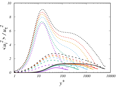
(a)  (b) 

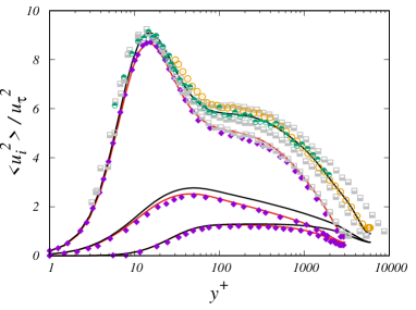
Figure 8: Distribution of velocity variances (a) and comparison of cases DNS-E, DNS-F with reference DNS and experiments (b). In panel (a), the short dashed lines denote the axial velocity variance ($<u_{z}^{2}>$), the solid lines denote the radial velocity variance ($<u_{r}^{2}>$), and the long dashed lines denote the azimuthal velocity variance ($<u_{\theta}^{2}>$). For color codes in DNS data, see table 1, and for nomenclature of symbols, see table 3.

The distributions of the velocity variances along the coordinate directions are shown in figure 8, in inner scaling. As now well established (Marusic & Monty, 2019), the longitudinal ($u_{z}$) and spanwise ($u_{\theta}$) velocity fluctuations show slow increase with the Reynolds number, with commonly accepted logarithmic growth as after Townsend’s attached eddy model (Townsend, 1976). On the other hand, the wall-normal velocity fluctuations seem to level off to a maximum value of about $1.30$. It is remarkable that the general growth of the longitudinal and spanwise fluctuations is more evident in the outer layer, and in fact it has long been argued about the possible occurrence of a secondary peak of $<u^{2}_{z}>$, besides the primary buffer-layer peak. Experiments carried out in the Superpipe (Hultmark et al., 2012) and CICLoPE (Willert et al., 2017) facilities indeed support the occurrence of such peak at $\Rey_{\tau}\gtrsim 10^{4}$. Whereas DNS data are not at sufficiently high $\Rey_{\tau}$ to show this secondary peak, it appears that in DNS-F the axial velocity variance has attained a nearly horizontal inflectional point at $y^{+}\approx 140$. Comparison with the $\Rey_{\tau}\approx 3000$ DNS of Ahn et al. (2015) shows overall good agreement of all turbulence intensities. Comparison with Superpipe data at $\Rey_{\tau}=3000$ is also very good, with exception of the near-wall peak which is likely to be over-estimated in experiments. DNS-F data seem to be well bracketed by Superpipe and CICLoPE measurements at nearby Reynolds numbers, and also compare very well with experimental data for plane channel flow (Schultz & Flack, 2013).

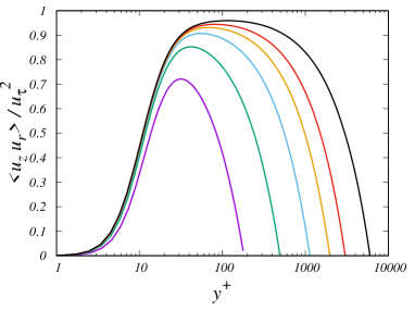
(a)  (b) 

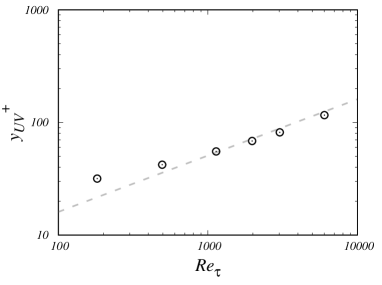
Figure 9: Distributions of turbulent shear stress (a) and its peak position at various $\Rey_{\tau}$ (b). The dashed line in panel (b) denotes the theoretical estimate (8). For color codes in DNS data, see table 1.

Distributions of the turbulent shear stress are shown in figure 9. As is well established (e.g. Lee & Moser, 2015), the shear stress profiles tend to become flatter at higher $\Rey_{\tau}$, the peak value rises towards unity, and its position moves farther from the wall, in inner units. In particular, exploiting mean momentum balance and assuming the presence of a logarithmic layer in the mean axial velocity, the following prediction follows for the position of the turbulent shear stress peak (Afzal, 1982)

$$y_{{}_{UV}}^{+}\approx\sqrt{\frac{\Rey_{\tau}}{k}},$$ (8)

which is intermediate between inner and outer scaling. This observation has led some authors to argue about the relevance of a ’mesolayer’ (Long & Chen, 1981; Wei et al., 2005). The asymptotic relationship (8) is satisfied with good accuracy starting at $\Rey_{\tau}\approx 10^{3}$, reflecting the onset of a near logarithmic layer.

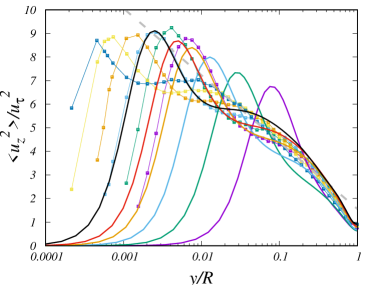
(a)  (b) 

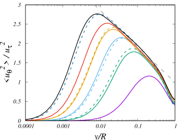
Figure 10: Axial (a) and azimuthal (b) turbulent stresses as a function of outer-scaled wall distance. In panel (a), symbols denote Superpipe data (Hultmark et al., 2012) at $\Rey_{\tau}=1985,3334,5411,10480,20250,37690$, and the dashed grey line the corresponding fit, $\left<u_{z}^{2}\right>=1.61-1.25\log(y/R)$. In panel (b), the dashed colored lines denote DNS data of channel flow (Lee & Moser, 2015) at $\Rey_{\tau}=550,1000,2000,5200$, and the dashed grey line the fit of the DNS data, $\left<u_{\theta}^{2}\right>=1.0-0.40\log(y/R)$. For color codes in DNS data, see table 1.

The behaviour of the Reynolds stresses when expressed as a function of the outer-scaled wall distance, which is shown in figure 10 is also of great theoretical interest. In fact, according to the attached-eddy model (Townsend, 1976; Marusic & Monty, 2019), the wall-parallel velocity variances are expected to decline logarithmically with the wall distance in the outer layer, hence

$$\left<u_{z}^{2}\right>=B_{1}-A_{1}\log(y/R),\quad\left<u_{\theta}^{2}\right>=B_{3}-A_{3}\log(y/R).$$ (9)

where $A_{i}$, $B_{i}$ are universal constants. Regarding the axial stress, Marusic et al. (2013) argued that Superpipe data at the highest available Reynolds number are best fit with $A_{1}=1.23$, $B_{1}=1.56$, with a sensible logarithmic layer only emerging at $\Rey_{\tau}>10^{4}$, in the range of wall distances $3\Rey_{\tau}^{1/2}\leq y^{+}\leq 0.15\Rey_{\tau}$. DNS data only show the formation of a near logarithmic layer farther away from the wall, which is not where it is expected from theoretical arguments. Hence, little can be said in this respect. The azimuthal velocity variance, shown in figure 10(b), has a more benign behaviour, and it features clear logarithmic layers even at modest $\Rey_{\tau}$. Fitting the DNS data yields $A_{3}=0.40$, $B_{3}=1.0$, which is very close to what found in channels (Bernardini et al., 2014; Lee & Moser, 2015). Measurements of pipe flow carried out in the CICLoPE facility (Örlü et al., 2017) yielded $A_{3}=0.63$, $B_{3}=1.21$, hence much larger values than in DNS. Possible overestimation of the wall-normal and azimuthal Reynolds stresses was in fact acknowledged by the authors of that paper.

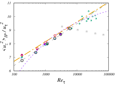
(a)  (b) 

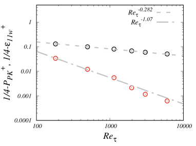
Figure 11: Magnitude of inner peak of axial velocity variance (a) and peak turbulence production ($P_{{}_{PK}}$, red), and wall dissipation of axial velocity variance ($\epsilon_{{}_{11w}}$, black) (b). For color codes in DNS data, see table 1, and for nomenclature of symbols, see table 3. In panel (a) the dashed grey line marks the DNS data fit, $<u^{2}_{z}>^{+}_{{}_{IP}}=0.67\log\Rey_{\tau}+3.3$, the dashed purple line denotes the defect power law of Chen & Sreenivasan (2021), and the dash-dotted line the logarithmic law of Marusic et al. (2017), $<u^{2}_{z}>^{+}_{{}_{IP}}=0.63\log\Rey_{\tau}+3.8$. In panel (b), the dot-dashed and dotted lines denote fits of $P_{{}_{PK}}$ and $\epsilon_{{}_{11w}}$ in their tendency to the respective assumed asymptotic values.

Quantitative insight into Reynolds number effects is provided by inspection of the amplitude of the inner peak of the axial velocity variance, which we show in figure 11. The general theoretical expectation is that the peak grows logarithmically with $\Rey_{\tau}$ owing to the increasing influence of distant, inactive eddies (Marusic & Monty, 2019). However, some recent experimental results (Willert et al., 2017), and theoretical arguments (Chen & Sreenivasan, 2021) suggest that such growth should eventually saturate. Although difference between slow logarithmic growth and attainment of an asymptotic value is quite subtle in practice, the theoretical interest is high as in the latter case universality of wall scaling would be eventually restored. Within the investigated range of Reynolds numbers, our DNS data in fact support continuing logarithmic increase. Comparison with channel data (Lee & Moser, 2015) shows some difference, which might result from stronger geometrical confinement of distant eddies in the pipe geometry. However, differences tend to becomes smaller at higher $\Rey_{\tau}$. In quantitative terms, we find the slope of logarithmic increase to be about $0.67$, a bit steeper than found in channel flow DNS (Lee & Moser, 2015, about $0.64$), and than suggested from a collection of DNS and experiments (Marusic et al., 2017, about $0.63$). Experimental data for pipe flow are quite scattered, as Superpipe experiments yield an unrealistically decreasing trend (Hultmark et al., 2012), PIV measurements taken in the CIPLoPE facility (Willert et al., 2017) suggest saturation of the growth, whereas hot-wire measurements in the same facility support continued logarithmic growth (Fiorini, 2017). The theoretical predictions of Chen & Sreenivasan (2021) (see the dashed purple line of figure 11a) seem to conform well with channel flow DNS data and with the experiments of Willert et al. (2017).

While our DNS data cannot be used to directly evaluate the theoretical predictions owing to limited achievable Reynolds number, they can be used to better scrutinize the foundations of the theoretical arguments. The main argument made by Chen & Sreenivasan (2021), although not thoroughly justified in our opinion, was that since turbulence kinetic energy production is bounded, the wall dissipation must also stay bounded. Hence, let $P=-\left<u_{z}u_{r}\right>\mathrm{d}U/\mathrm{d}r$ be the turbulence kinetic energy production rate, and $\epsilon_{11}=\nu\left<\left|\nabla u_{z}\right|^{2}\right>$ be the dissipation rate of the axial velocity variance, those authors first argue that the wall limiting value of $\epsilon_{11}$ should scale as

$${\epsilon_{11}}_{w}^{+}=1/4-\beta/\Rey_{\tau}^{1/4},$$ (10)

with $\beta$ a suitable constant. In figure 11 we explore deviations of $\epsilon_{w}$ and of the peak turbulence kinetic energy production, say $P_{{}_{PK}}$, from their asymptotic value, namely $1/4$. According to analytical constraints (Pope, 2000), we find that production tends to its asymptotic value quite rapidly, as about $1/\Rey_{\tau}$. Consistent with equation (10), the wall dissipation also tends to $1/4$, more or less at the predicted rate, thus empirically validating the first assumption. The next argument advocated by Chen & Sreenivasan (2021) is that wall balance between viscous diffusion and dissipation and Taylor series expansion of the axial velocity variance near the wall yields

$$\left<u_{z}^{2}\right>^{+}\sim\epsilon_{{}_{11w}}^{+}{y^{+}}^{2},$$ (11)

whence, from assumed invariance of the peak location of $\left<u_{z}^{2}\right>$ (say, $y_{{}_{IP}}^{+}$), saturation of growth of the peak velocity variance would follow. Table 2 suggests that this second assumption is in fact violated, as the position of the peak slightly increases with $\Rey_{\tau}$, with non-negligible effect on the peak variance as it appears in squared form in equation (11). As a consequence, logarithmic growth of the peak velocity variance still holds, at least in the range of Reynolds numbers currently accessible to DNS.

(a) 

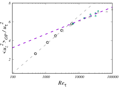
Figure 12: Magnitude of outer peak of axial velocity variance as a function of $\Rey_{\tau}$. Lines and symbols as in tables 1 and 3. The dashed grey line marks the DNS data fit, $\left<u_{z}^{2}\right>^{+}_{OP}=1.33\log\Rey_{\tau}-5.61$, and the purple line denotes the logarithmic fit given by Pullin et al. (2013).

Although no distinct outer peak of the axial velocity variance is found at the Reynolds numbers under scrutiny, it is nevertheless instructive to explore the scaling of the velocity fluctuations in the range of wall distances where the peak is expected to occur. For that purpose, we consider the outer position where the second logarithmic derivative of the velocity variance vanishes, which in the present DNS ranges from $y^{+}\approx 115$ for DNS-A, to $y^{+}\approx 140$ for DNS-F. Weak dependence of the inner-scaled outer peak position on $\Rey_{\tau}$, although at much higher Reynolds number, was also noticed by Hultmark et al. (2012). The resulting distribution is shown in figure 12. All DNS data fall nicely on a logarithmic fit, and they seem to connect smoothly to the experimental results, whose scatter and uncertainty is expected to be much less than for the inner peak. Experiments indicate a change of behaviour to a shallower logarithmic dependence with slope of about $0.63$ (Fiorini, 2017; Pullin et al., 2013), which would be very close to the growth rate of the inner peak (see figure 11). The figure suggests that verification of this effect would require $\Rey_{\tau}$ of about $10^{4}$.

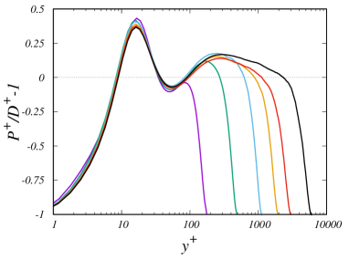
(a)  (b) 

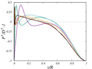
Figure 13: Excess of turbulence kinetic energy production over dissipation as a function of inner-scaled (a) and outer-scaled (b) wall distance. Lines as in table 1.

As pointed out by Hultmark et al. (2012), the formation and growth of an outer peak of the axial velocity variance has important theoretical and practical implications. From the modeling standpoint, no current RANS model is capable of predicting non-monotonic behaviour of Reynolds stresses outside the buffer layer. From the fundamental physics standpoint, the presence of an outer peak is suggestive of violation of equilibrium between turbulence production and dissipation, thus invalidating one of the possible arguments advocated for the formation of a logarithmic mean velocity profile (Townsend, 1976). DNS allows to substantiate this scenario, and for that purpose in figure 13, we show the relative excess of turbulent kinetic energy production ($P$) over its total dissipation rate, here defined as $D=\nu\left<u_{i}\nabla^{2}u_{i}\right>$, which lumps together dissipation rate and viscous diffusion. Data confirm the presence of a near-universal region confined to the buffer layer (say, $8\lesssim y^{+}\lesssim 35$), in which production exceeds dissipation by up to $40\%$. Data also show the onset, starting from DNS-B, of another region farther from the wall with positive unbalance, whose inner limit is constant in inner units, at $y^{+}=100$, and whose outer limit tends to become constant at high $\Rey_{\tau}$ in outer units, at $y/R\approx 0.4$. The peak unbalance at high Reynolds number is about $17\%$, and its position seems to scale more in inner than in outer units. Turbulence kinetic energy production excess in the presence of a (near) logarithmic mean velocity profile can be interpreted by recalling that only part of the kinetic energy which is being generated is converted to active motions which carry turbulent shear stress, and the rest is used to feed inactive motions. This finding clearly indicates that at high enough Reynolds number the outer wall layer becomes a dynamically active part of the flow, having the potential to transfer energy both to the core flow, and towards the wall, in the form of imprinting on the near-wall layer (Marusic & Monty, 2019).

4 Concluding comments

Although DNS of wall turbulence is still confined to a moderate range of Reynolds numbers, it is beginning to approach a state in which some typical phenomena of the asymptotically high-$\Rey$ emerge. Given its ability to resolve the near-wall layer, DNS lends itself to testing theories of wall turbulence and to in-depth scrutiny of experimental data. In this work, DNS of flow in a smooth pipe has been carried out up to $\Rey_{\tau}\approx 6000$, which, although still far from what achievable in experimental tests, allows to uncover a number of interesting issues, in our opinion. First, we have noted that DNS data fall systematically short of the classical Prandtl friction law, by as much as $2\%$. This evidence is not consistent with data from the Superpipe facility, although other recent data from the CICLoPE and Hi-Reff facilities seem to yield similar trends. DNS data fitting suggests that a logarithmic law as (2) still holds, however with a von Kármán constant $k\approx 0.387$, which matches extremely well the value quoted by Furuichi et al. (2018), and which would reconcile pipe flow with plane channel and boundary layer flows, thus corroborating claims made by Marusic et al. (2013). A logarithmic profile with $k\approx 0.387$ well fit the mean axial velocity distributions for $30\leq y^{+}\leq 0.15\Rey_{\tau}$, although linear deviations are clearly visible, as argued by Afzal & Yajnik (1973); Luchini (2017), which is taken into account yield excellent representation of the velocity profiles up to $y/R\approx 0.5$. It is remarkable that the same value of the von Kármán constant also well fits the mean centerline velocity distribution (see figure 7), which is found to grow logarithmically throughout the range of $\Rey_{\tau}$ under investigation. This finding is quite reasonable as it corroborates that the eventual state of turbulent flow in a pipe should be plug flow, as argued by Pullin et al. (2013), hence $U_{{}_{CL}}\to u_{b}$ as $\Rey_{\tau}\to\infty$. This would however seemingly contrast recent measurements made in the CICLoPE facility (Nagib et al., 2017), which rather suggest a different von Kármán constant for the bulk and the centerline velocity. Experimental data at $\Rey_{\tau}\gtrsim 10^{4}$ in fact suggest deviations of $U_{{}_{CL}}^{+}$ from the logarithmic trend found DNS, however this effect requires further confirmation, as data are quite scattered. The core velocity profile is found to be to a good approximation parabolic, with curvature which is nearly constant in wall units, and decreasing in outer units.

Regarding the velocity fluctuations, we find evidence for continuing logarithmic increase of the inner-peak magnitude with $\Rey_{\tau}$. Some experiments and theoretical arguments would indicate that beyond $\Rey_{\tau}\approx 10^{4}$ a change of behaviour might occur, which however is very difficult to quantify. DNS is probably of little use in this respect, as in order to clearly discern among the various trends, $\Rey_{\tau}$ in excess of $10^{5}$ are likely to be needed. As predicted by the attached-eddy hypothesis, the wall-parallel velocity variances in the outer layer tend to form logarithmic layers, which are especially evident in the azimuthal velocity. Although we do not find direct evidence for the existence of an outer peak of the axial velocity variance, our results highlight the occurrence of an outer site with substantial turbulence production excess over dissipation, thus contradicting the classical equilibrium hypothesis and likely to yield a distinct peak at $\Rey_{\tau}\approx 10^{4}$, as Superpipe and CICLoPE experiments suggest. Investigating these and other violations of universality of wall turbulence to extrapolate asymptotic behaviours is a formidable challenge for theoreticians in years to come.

[Acknowledgments] We acknowledge that the results reported in this paper have been achieved using the PRACE Research Infrastructure resource MARCONI based at CINECA, Casalecchio di Reno, Italy, under project PRACE n. 2019204979. Discussions with A.J. Smits are gratefully acknowledged. We would like to thank P. Luchini and M. Quadrio for providing the code used for the data uncertainty analysis.

[Funding]This research received no specific grant from any funding agency, commercial or not-for-profit sectors.

[Declaration of interests]The authors report no conflict of interest.

[Data availability statement]The data that support the findings of this study are openly available at the web page http://newton.dma.uniroma1.it/database/

References

- Afzal (1982) Afzal, N. 1982 Fully developed turbulent flow in a pipe: an intermediate layer. Ingenieur-Archiv 52 (6), 355–377.
- Afzal & Yajnik (1973) Afzal, N. & Yajnik, K. 1973 Analysis of turbulent pipe and channel flows at moderately large Reynolds number. J. Fluid Mech. 61, 23–31.
- Ahn et al. (2013) Ahn, J., Lee, J.H., Jang, S. & Sung, H.J. 2013 Direct numerical simulations of fully developed turbulent pipe flows for Re and . Int. J. Heat Fluid Fl. 44, 222–228.
- Ahn et al. (2015) Ahn, J., Lee, J.H., Lee, J., Kang, J.-H. & Sung, H.J. 2015 Direct numerical simulation of a 30R long turbulent pipe flow at Re. Phys. Fluids 27, 065110.
- Akselvoll & Moin (1996) Akselvoll, K. & Moin, P. 1996 An efficient method for temporal integration of the Navier–Stokes equations in confined axisymmetric geometries. J. Comput. Phys. 125, 454–463.
- Barenblatt et al. (1997) Barenblatt, GI, Chorin, AJ & Prostokishin, VM 1997 Scaling laws for fully developed turbulent flow in pipes. Appl. Mech. Rev. 50, 413–429.
- Bernardini et al. (2014) Bernardini, M, Pirozzoli, S & Orlandi, P 2014 Velocity statistics in turbulent channel flow up to Re. J. Fluid Mech. 742, 171–191.
- Cantwell (2019) Cantwell, B.J. 2019 A universal velocity profile for smooth wall pipe flow. J. Fluid Mech. 878, 834–874.
- Chen & Sreenivasan (2021) Chen, X. & Sreenivasan, K.R. 2021 Reynolds number scaling of the peak turbulence intensity in wall flows. J. Fluid Mech. 908, R3.
- Chin et al. (2014) Chin, C, Monty, JP & Ooi, A 2014 Reynolds number effects in DNS of pipe flow and comparison with channels and boundary layers. Int. J. Heat Fluid Fl. 45, 33–40.
- Chin et al. (2010) Chin, Cheng, Ooi, ASH, Marusic, Ivan & Blackburn, HM 2010 The influence of pipe length on turbulence statistics computed from direct numerical simulation data. Phys. Fluids 22 (11), 115107.
- Durst et al. (1995) Durst, F, Jovanović, J & Sender, J 1995 LDA measurements in the near-wall region of a turbulent pipe flow. J. Fluid Mech. 295, 305–335.
- Eggels et al. (1994) Eggels, JGM, Unger, F, Weiss, MH, Westerweel, J, Adrian, RJ, Friedrich, R & Nieuwstadt, FTM 1994 Fully developed turbulent pipe flow: a comparison between direct numerical simulation and experiment. J. Fluid Mech. 268, 175–210.
- El Khoury et al. (2013) El Khoury, GK, Schlatter, P, Noorani, A, Fischer, PF, Brethouwer, G & Johansson, AV 2013 Direct numerical simulation of turbulent pipe flow at moderately high Reynolds numbers. Flow Turbul. Combust. 91, 475–495.
- Fiorini (2017) Fiorini, T. 2017 Turbulent pipe flow - high resolution measurements in ciclope. PhD thesis, School of Engineering and Architecture, University of Bologna.