Are energy savings the only reason for the emergence
of bird echelon formation?

Abstract

We analyze the conditions under which the emergence of frequently observed echelon formation can be explained solely by the maximization of energy savings. We consider a two-dimensional multi-agent echelon formation, where each agent receives a benefit that depends on its position relative to the others, and adjusts its position to increase this benefit. We analyze the selfish case where each agent maximizes its own benefit, leading to a Nash-equilibrium problem, and the collaborative case in which agents maximize the global benefit of the group. We provide conditions on the benefit function under which the frequently observed echelon formations cannot be Nash equilbriums or group optimums.

We then show that these conditions are satisfied by the conventionally used fixed-wing wake benefit model. This implies that energy saving alone is not sufficient to explain the emergence of the migratory formations observed, based on the fixed-wing model. Hence, either non-aerodynamic aspects or a more accurate model of bird dynamics should be considered to construct such formations.

I introduction

Formation control where multiple agents collaborate to move in certain shapes received extensive interest in the literature, see e.g., the survey [1]. Different methods based on available sensor measurements, e.g., position [2, 3], distance [4, 5] and bearing [6, 7], have been proposed to achieve formations for various agent dynamics. There is also a research line focusing on imitating the collective behavior of animals, e.g., birds flock or fish school, by designing simple local interaction rules [8]-[11]. Despite these fruitful results, the existing researches mostly focus on the actions agents take in order to form and maintain specific shapes, or on how phenomenological behavior models may result in formation-like behaviors. But, the benefits of these formations and their influence on the emergence of formations are rarely addressed.

In nature, several animal species, e.g., birds, fish and lobsters, move in specific formations that are argued to be caused by energy saving [12]. In particular, it is well-acknowledged that migrating birds adopt the eye-catching line formation because each follower bird reduces energy expenditure by exploiting the extra supportive lift from the wake of the front neighboring bird [13]-[15]. By regarding birds as fixed wings, early researches [15]-[18] have tested the energy saving mechanism. Though the predicted relative position of neighboring birds is consistent with the observations of migrating birds, the position of each bird was always pre-fixed, without considering birds’ incentive to pick the preferred position. Some papers in the last decade [19, 20] also seek to construct line formations based on modified fixed wing models. However, their modification violates the wake evolution in aircraft experiments [21], hence the conclusion could be questioned. Moreover, other non-aerodynamic factors are also considered in these work. Hence the actual emergence of the specific formation shapes (echelon or V) remains unexplained on multiple aspects, such as birds interests in energy saving, sensing ability, and action strategies. A first fundamental question is whether migrating formations emerge purely based on energy saving? To answer this, in [22] we have recently tried employing the fixed-wing model to numerically constructing the echelon formation for birds by assuming all of them are either selfish or cooperative in energy optimization; see Section II-B for more detailed explanation about these behaviors. Surprisingly, no observation-similar echelon formation has been found in any of the situations.

Our contribution in this paper is to theoretically confirm this result. We study the general two-dimensional multi-agent echelon formations based on benefit optimization. In our setting, each agent can receive from any other agent a benefit that depends on its relative position to that agent. A leader is fixed at the front of the group, while other followers can adjust their positions and their behaviors are purely guided by benefit optimization. Same as in our trial in constructing migratory formations, we consider that all agents are either selfish or cooperative, resulting in a self-benefit maximization non-cooperative game or a cooperative total benefit optimization problem, respectively. Related to the emergence of echelon formations, our focus is to derive conditions of the inter-agent benefit, under which there cannot exist a Nash equilibrium of the self-benefit game and/or the (local) optimum of the total benefit optimization, at which the relative position of each neighboring-agents lies within some proper set.

This question is close to constrained non-cooperative games and maximization, where the existence of equilibriums or optimums could be guaranteed by requiring objective functions to be continuous or concave [23, 24]. But, unlike these problems, we focus on whether the unconstrained game or maximization has some equilibriums or optimums that are within the desired set by coincidence.

We derive several results by analyzing the necessary condition of the existence of the Nash equilibrium and/or the maximum. Based on these results, we confirm the numerical results in [22] using the fixed-wing model that birds behaving purely to maximize energy savings may not be sufficient to create the migratory formation.

The rest of the paper is organized as follows: In the next section, we first explain echelon formations, the benefit optimization problems with different birds interests and the considered Nash equilibrium and optimum. Then, we formulated the problem of interest. Section III and IV present conditions on the inter-agent benefit such that the considered Nash equilibrium and optimum, respectively, cannot exist. In Section V, we apply the proposed theoretical conditions to analyzing the fixed-wing wake model and justify our numerical results. At last, Section VI concludes the paper and discuss the implication of the results. The Appendix provides the proof for an intermediate result in Section VI.

II Preliminaries

II-A Notations

Let $\text{Id}(\cdot)$ be the identity map. For a negative interval $\mathcal{P}\subset\mathbb{R}_{-}$, we denote by $-\mathcal{P}$ and $2\mathcal{P}$ the image of $-\text{Id}(a)$ and $2\text{Id}(a)$ when $a\in\mathcal{P}$, respectively. For a differentiable function $f(x):\mathbb{R}^{m}\rightarrow\mathbb{R},m\geq 2$, we denote by $\frac{\partial f(x^{*})}{\partial x_{i}}=\frac{\partial f(x)}{\partial x_{i}}|_{x=x^{*}}$ the partial derivative of $f(x)$ with respect to the $i$th component of the argument at $x^{*}\in\mathbb{R}^{m}$. Moreover, if $m=2$, we denote $f_{x}(a,b)=\frac{\text{d}f(x,b)}{\text{d}x}|_{x=a}$, with $a,b\in\mathbb{R}$ before Section V.

II-B Echelon formation, agents benefits and interests

We consider $n+1$ agents with one leader with label 0, and $n\geq 2$ followers labeled from 1 to $n$. Let $V=\{1,...,n\}$ denote the set of followers. For each agent $i\in V\cup\{0\}$, we call agent $j$, with $j=i\mp k\geq 0$ with $1\leq k\leq n$, the $k$-hop front (back) neighbor of $i$. ${\mathcal{N}}_{i}\subset V\cup\{0\}$ denotes the set of $1$- and $2$-hop neighbors of $i$. Each agent $i\in V\cup\{0\}$ has a position $p_{i}=[x_{i}\ y_{i}]^{\top}\in\mathbb{R}^{2}$ and specifically $p_{0}=0_{2}$ in this paper. Let $X=[x_{1}\ ...\ x_{n}]^{\top}$, $Y=[y_{1}\ ...\ y_{n}]^{\top}$ and $p=[X^{\top}\ Y^{\top}]^{\top}$. In the later, the $x$ and $y$ directions are also called the longitudinal and lateral directions, respectively. Backward motion means moving at the negative $x$ direction. Let $p_{ij}=p_{i}-p_{j}$ and $x_{ij}=x_{i}-x_{j}$ for any unequal $i,j\in V\cup\{0\}$.

Each agent $i\in V\cup\{0\}$ can gain a benefit $f^{(i)}(p)$ that depends on agents positions $p$, from all others. Consistently with the analysis of bird formations [13], where the energy saving of the bird is additive and each bird is affected mostly by two front and back birds, we assume that $f^{(i)}(p)$ can be decomposed as the sum of the benefits $f(p_{ij})$ agent $i$ gets from $j\in\mathcal{N}_{i}$, where $f(\cdot):\mathbb{R}^{2}\rightarrow\mathbb{R}$ is the inter-agent benefit. Mathematically,

$$f^{(i)}(p)=\sum_{j\in{\mathcal{N}}_{i}}f(p_{ij})=\sum_{j\in V\cup\{0\}}^{|i-j|\leq 2,\ i\neq j}f(p_{ij})$$ (1)

The total benefit $J(p)$ of the group is then the sum of the benefit of all agents:

$$J(p) =\sum_{i\in V\cup\{0\}}f^{(i)}(p)=\sum_{i\in V\cup\{0\}}\sum_{j\in{\mathcal{N}}_{i}}f(p_{ij})$$ (2)

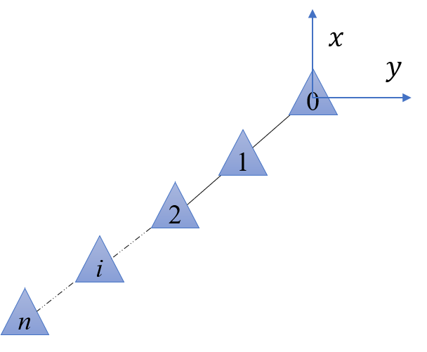
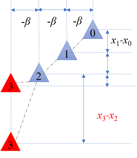
Figure 1: Echelon formation and formations that are weird. (a) $n+1$ agents create an echelon formation in a plane. (b) Weird formation that should be excluded. Agent $3$ in red color is either too close or too far from the front neighbor longitudinally.

We focus on echelon formations as shown in Fig. 1, where agents are aligned diagonally behind the leader in one side with equal neighboring-agents distance. Motivated by the line formation of migrating birds where neighboring birds’ lateral distances are almost the same but longitudinal distances are varied within proper range [13, 15], we allow the formation to be deviated from the strict echelon shape. Specifically, we focus on the left echelon formation where the position $p_{i}$ of each follower $i\in V$ satisfies

$$y_{i}=-i\beta,\quad x_{i(i-1)}\in\mathcal{P}$$ (3)

where $\beta$ is a positive and $\mathcal{P}=[-\alpha_{l},-\alpha_{s}]$ with $\alpha_{s},\alpha_{l}$ two preset positives satisfying $\alpha_{s}\leq\alpha_{l}$. Let $Y(\beta)=[-\beta\ ...\ -n\beta]^{\top}$. Then $f^{(i)}(p)$ and $J(p)$ can also be denoted as $f^{(i)}(X,Y(\beta))$ and $J(X,Y(\beta))$, respectively.

In the paper, we fix $\beta$ and consider to construct the echelon formation of interest by assuming that followers can adjust their longitudinal position $x_{i}$ based on benefit maximization. Two different agent attitudes are considered. In the first, all followers are selfish and would like to maximize their own benefits $f^{(i)}(p)$. This leads to a non-cooperative game and we are interested in the Nash equilibrium (NE) of the longitudinal positions, which is defined as the vector $X^{*}=[x^{*}_{1}\ \cdots\ x^{*}_{n}]^{\top}\in\mathbb{R}^{n}$ satisfying the condition below for each $i\in V$:

$$f^{(i)}(x_{i}^{*},x_{-i}^{*},Y(\beta))\leq f^{(i)}(x_{i},x_{-i}^{*},Y(\beta)),\quad\forall x_{i}\in\mathbb{R}$$ (4)

where $x^{*}_{-i}=[x_{1}^{*}\ \cdots\ x_{i-1}^{*}\ x_{i+1}^{*}\ \cdots\ x_{n}^{*}]^{\top}$. The NE, if exists, corresponds to agents longitudinal positions with the property that no agent can increases its own benefit by choosing a different position unilaterally.

In the second, all agents cooperative to maximize the group total benefit $J$ and we are interested in the cooperative equilibrium (CE), which is the vector of agents’ longitudinal positions $\bar{X}^{*}=[\bar{x}^{*}_{1}\ \cdots\ \bar{x}^{*}_{n}]^{\top}\in\mathbb{R}^{n}$ that reaches a local maximum of $J$.

$$\bar{X}^{*}:=\arg\max_{X\in\mathcal{B}_{X}}J(p)=\arg\max_{X\in\mathcal{B}_{X}}J(X,Y(\beta))$$ (5)

where $\mathcal{B}_{X}$ is a neighborhood of $X$. It is proper to consider the local maximum since without prior knowledge of the global maximum, the cooperative followers have no incentive to shift away from a local maximum. Moreover, the global maximum is also a local maximum, thereby satisfies (5).

We denote $p_{i}^{*}=[x_{i}^{*}\ -i\beta]^{\top}$, $\bar{p}_{i}^{*}=[\bar{x}_{i}^{*}\ -i\beta]^{\top}$, $p^{*}=[(X^{*})^{\top}\ Y(\beta)^{\top}]^{\top}$, and $\bar{p}^{*}=[(\bar{X}^{*})^{\top}\ X(\beta)^{\top}]^{\top}$, respectively. Consistently with the considered echelon formation, we only focus on the NE $X^{*}$ and CE $\bar{X}^{*}$ with $x^{*}_{i(i-1)}\in\mathcal{P},i\in V$ and $\bar{x}^{*}_{i(i-1)}\in\mathcal{P},i\in V$, respectively, for a negative closed interval $\mathcal{P}$ and positive $\beta$, which can be preset based on practical tasks or observations. Whether a considered echelon formation can be constructed based on benefit maximization should relate to if there exist the equilibrium of interest.

II-C Problem formulation

In view of $f^{(i)}(p)$ and $J(p)$, the existence of $X^{*}$ and $\bar{X}^{*}$ should depend on the properties of the inter-agent benefit $f$. By imposing strong concavity [24] on the benefit within the interval $\mathcal{P}$, it might not be difficult to obtain conditions that guarantee the existence of the equilibrium of interest. While, in our efforts to reconstruct the migratory formation of birds based purely on benefit maximization, no equilibrium that corresponds to observation-similar echelon formation has been found. To explain this, we focus on the following problem in the paper.

Problem 1. Given $n\geq 2$ agents, an interval $\mathcal{P}=[-\alpha_{l},-\alpha_{s}]$ with $0<\alpha_{s}\leq\alpha_{l}$ and a $\beta>0$, under what conditions on $f$, the NE $X^{*}\in\mathbb{R}^{n}$ with $x^{*}_{i(i-1)}\in\mathcal{P},i\in\mathcal{V}$ and/or the CE $\bar{X}^{*}\in\mathbb{R}^{n}$ with $\bar{x}^{*}_{i(i-1)}\in\mathcal{P},i\in V$ are impossible.

At this stage, we impose the following assumption on the inter-agent benefit $f$, allowing to consider its derivative.

Assumption 1

(a) $f(x,y)$ with $x,y\in\mathbb{R}$ is continuous in $\mathbb{R}^{2}$ and is continuously differentiable when $x\neq 0$ (b) $f(x,y)=f(x,-y)$ for $x,y\in\mathbb{R}$.

The continuity of the derivative of $f$ is not assumed at $x=0$ since the inter-agent benefit may have an acute change when an agent shifts from the back to the front of another agent longitudinally.

Note that $f(p_{ij})$ takes $p_{ij}=[x_{ij}\ y_{ij}]^{\top}$ and remember the definition of the NE in (5). Then by the chain rule, if a NE $X^{*}$ with $x^{*}_{i(i-1)}\in\mathcal{P},i\in V$ exists, it should satisfy the equation below for each $i\in V$

$$0=\frac{\partial f^{(i)}(p^{*})}{\partial x_{i}}=\sum_{j\in{\mathcal{N}}_{i}}\frac{\partial f(p_{ij})}{\partial x_{ij}}\frac{\partial x_{ij}}{\partial x_{i}}\biggr{|}_{p^{*}}=\sum_{j\in{\mathcal{N}}_{i}}\frac{\partial f(p_{ij}^{*})}{\partial x_{ij}}$$ (6)

By contrast, if a CE $\bar{X}^{*}$ with $\bar{x}^{*}_{i(i-1)}\in\mathcal{P},i\in V$ exists, it should satisfy the following equation for each $i\in V$

$$0=\frac{\partial J(\bar{p}^{*})}{\partial x_{i}} =\sum_{k\in V\cup\{0\}}\sum_{j\in{\mathcal{N}}_{k}}\frac{\partial f(p_{kj})}{\partial x_{kj}}\frac{\partial x_{kj}}{\partial{x_{i}}}\biggr{|}_{\bar{p}^{*}}$$

$$=\sum_{j\in{{\mathcal{N}}_{i}}}\frac{\partial f(\bar{p}_{ij}^{*})}{\partial x_{ij}}-\frac{\partial f(\bar{p}_{ji}^{*})}{\partial x_{ji}}$$ (7)

where the last equality is from (1) and (2).

Hence, checking if the equilibriums of interest exist is equivalent to testing if there exist a solution $X^{*}$ with $x_{i(i-1)}^{*}\in\mathcal{P},i\in V$ to equation (6) and/or a solution $\bar{X}^{*}$ with $\bar{x}_{i(i-1)}^{*}\in\mathcal{P},i\in V$ to (II-C), respectively.

III Nonexistence of the NE of interest

In this section, we focus on the selfish case and discuss the conditions on $f$ such that there exists no NE of interest.

III-A Three agents case

We first consider the simple case of three agents, 1 leader and 2 followers and $V=\{1,2\}$). Intuitively, if the increment of agent 1’s benefit from its back neighbor (agent 2) is more than its benefit loss from the front neighbor (agent 0) when agent 1 moves backward, then agent 1 would like to move backward to get more benefit. If this always holds when $x_{21},x_{10}\in\mathcal{P}$, then agent $1$ cannot be static when $x_{21},x_{10}\in\mathcal{P}$. In other words, the NE of interest cannot exist. The theorem below formulates this intuition.

Theorem 1

For $n=2$, $\beta>0$, a closed interval $\mathcal{P}\subset\mathbb{R}_{-}$, if $f(\cdot)$ satisfies Assumption 1 and

$$\max_{x\in-\mathcal{P}}f_{x}(x,-\beta)<-\max_{x\in\mathcal{P}}f_{x}(x,-\beta)$$ (8)

then there exists no NE $X^{*}\in\mathbb{R}^{2}$ with $x^{*}_{10},x^{*}_{21}\in\mathcal{P}$.

Proof. Suppose the conclusion is incorrect and there exists an NE $X^{*}\in\mathbb{R}^{2}$ satisfying $x_{10}^{*},x_{21}^{*}\in\mathcal{P}$. Since $f$ is continuously differentiable when $x\neq 0$ by Assumption 1(a), $X^{*}$ should satisfy (6).

Consider $i=1$ and notice that ${\mathcal{N}}_{1}=\{0,2\}$ and $p_{i}^{*}=[x_{i}^{*}\ -\beta]^{\top}$, (6) leads us to

$$f_{x}(x_{10}^{*},-\beta)+f_{x}(x_{12}^{*},\beta)=0$$

By $x^{*}_{10}\in\mathcal{P}$, $x_{12}^{*}\in-\mathcal{P}$ and Assumption 1(b), condition (8) leads us to $f_{x}(x_{12}^{*},\beta)<-f_{x}(x_{10}^{*},-\beta)$, contradicting the equality above. Hence, there exists no such $X^{*}$.  $\blacksquare$

Theorem 1 is based on the analysis of agent 1. If we consider benefit change of both agents 1 and 2, a different result can be obtained. Consider just agent 1 and 2, namely, $f^{(2)}(p)=f(p_{21})$. If $f(x,-\beta)$ peaks at $x=-\alpha$, then agent 2 should be $\alpha$ behind agent 1. Now take the leader 0 into account, namely $f^{(2)}(p)=f(p_{21})+f(p_{20})$. If $f(p_{20})$ changes very little when agent $2$ moves along the longitudinal direction, then the best $x_{21}$ that maximizes $f^{(2)}(p)$ would deviate very little from $-\alpha$. Hence when agent 1 moves longitudinally, if agent 2 wants to maximize the benefit, it should also move such that $x_{21}$ is within a very narrow interval $\mathcal{Q}\ni-\alpha$. Suppose this is true and $x_{12}\in-\mathcal{Q}$ always holds. Now assume that the increment of agent 1’s benefit from agent 2 is more than the decrement of its benefit from agent 0 when agent 1 moves backward but keeps $x_{10}\in\mathcal{P}$, then agent $1$ would like to move backward, until $x_{10}\notin-\mathcal{P}$. This implies that there exists no NE $X^{*}$ with $x_{i(i-1)}\in\mathcal{P},i\in\mathcal{V}$. This analysis can be formulated as another result, whose rigorous presentation relies on an assumption and several notations in the following.

Assumption 2

(a) $f(x,-\beta)$ has a global maximum $-\alpha$, and is strictly increasing when $x<-\alpha$ and strictly decreasing when $x>-\alpha$. (b)The global maximum is in the interval of interest, $-\alpha\in\mathcal{P}$.

Assumption 2(a) can be regarded as the attribute of the benefit $f$. It is mild and satisfied by at least the benefit considered in Section V. Assumption 2(b) relates to the choice of the interval $\mathcal{P}$. It is reasonable since otherwise a trivial conclusion could be obtained for the case of two agents that the follower 1 would never stay statically behind the leader 0, with $x_{10}\in\mathcal{P}$.

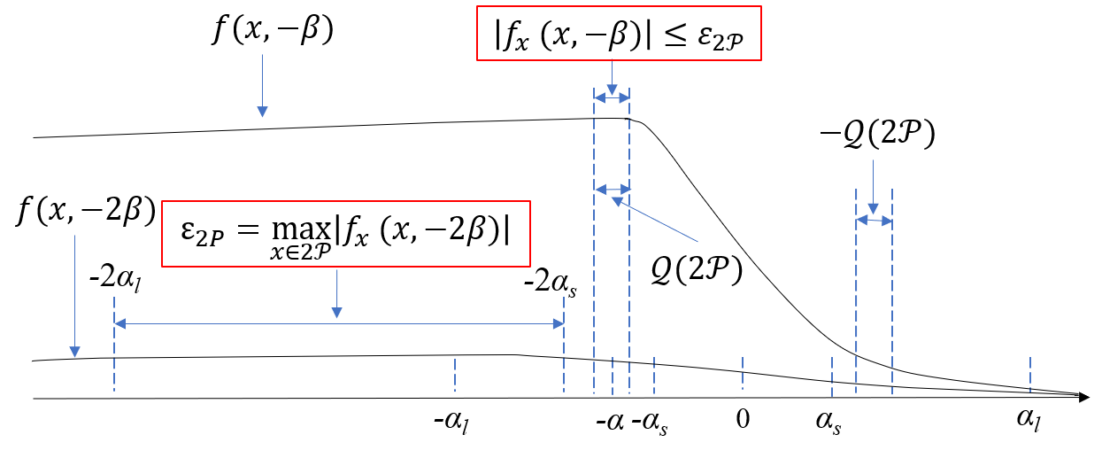
Figure 2: Illustration of $f$, $\varepsilon_{2\mathcal{P}}$ and $\mathcal{Q}(2\mathcal{P})$, where $f(x,-2\beta)$ is flat in $2\mathcal{P}$.

We then characterize the narrow interval around $-\alpha$ mentioned in the intuitive analysis before Assumption 2. For any non-empty closed interval ${\mathcal{I}}$, we denote

$$\varepsilon_{\mathcal{I}}:=\max_{x\in{\mathcal{I}}}\left|f_{x}(x,-2\beta)\right|$$ (9)

and let

$$\mathcal{Q}(\mathcal{I})=\{x\in\mathcal{P}|\left|f_{x}(x,-\beta)\right|\leq\varepsilon_{\mathcal{I}}\}$$ (10)

When $\mathcal{I}=2\mathcal{P}$, $\mathcal{Q}(\mathcal{I})$ relates to the narrow interval around $-\alpha$, though it may cover that. See Fig. 2 to get some vision of $\mathcal{Q}(2\mathcal{P})$. Formalizing the intuitive analysis, we have the following result.

Theorem 2

For $n=2$, $\beta>0$ and $\mathcal{P}=[-\alpha_{l},-\alpha_{s}]$ with $0<\alpha_{s}\leq\alpha_{l}$, assume that $f$ satisfies Assumption 1 and 2. If

$$\max_{x\in-\mathcal{Q}(\mathcal{I})}f_{x}(x,-\beta)<-\max_{x\in\mathcal{P}}f_{x}(x,-\beta)$$ (11)

with $\mathcal{I}=2\mathcal{P}$, then there exists no NE $X^{*}\in\mathbb{R}^{2}$ with $x^{*}_{10},x^{*}_{21}\in\mathcal{P}$.

Proof. First, the set $\mathcal{Q}(2\mathcal{P})$ is non-empty. In fact, since the maximum $-\alpha\in\mathcal{P}$ and $f_{x}$ is continuously for $x\neq 0$ by Assumption 1 and 2, for any small $\varepsilon_{\mathcal{I}}>0$, there should exist a neighborhood $\mathcal{B}_{-\alpha}$ of $-\alpha$ such that $|f_{x}(x,-\beta)|\leq\varepsilon_{\mathcal{I}}$ for all $x\in\mathcal{B}_{-\alpha}$. We always have $\mathcal{Q}(\mathcal{I})\supseteq\mathcal{B}_{-\alpha}\cap\mathcal{P}$.

Then, suppose there exists the NE $X^{*}\in\mathbb{R}^{2}$ of interest, a point satisfying (6). Notice that $\mathcal{N}_{1}=\{0,2\},\mathcal{N}_{2}=\{0,1\}$ and $p_{i}^{*}=[x_{i}^{*}\ -i\beta]^{\top}$, hence (6) becomes

$$0 =f_{x}(x_{10}^{*},-\beta)+f_{x}(x_{12}^{*},\beta)$$ (12)

$$0 =f_{x}(x_{20}^{*},-2\beta)+f_{x}(x_{21}^{*},-\beta)$$ (13)

Since $x_{10}^{*},x_{21}^{*}\in\mathcal{P}$, $x_{20}^{*}=x^{*}_{10}+x^{*}_{21}\in 2\mathcal{P}$, then from (9), $|f_{x}(x_{20}^{*},-2\beta)|\leq\varepsilon_{2\mathcal{P}}$. From equation (13), we also have $|f_{x}(x_{21}^{*},-\beta)|\leq\varepsilon_{2\mathcal{P}}$. Hence $x_{21}^{*}\in\mathcal{Q}(2\mathcal{P})$, or $x_{12}^{*}\in-\mathcal{Q}(2\mathcal{P})$. Then by (11) and Assumption 1(b), $f_{x}(x_{12}^{*},\beta)<-f_{x}(x_{10}^{*},-\beta)$. However, this leads to a contradiction since the left side of (12) would be negative.  $\blacksquare$

In Theorem 2, condition (11) should be satisfied for $\mathcal{I}=2\mathcal{P}$. Based on the analysis before Assumption 2, it may implicitly require the variation of $f(x,-2\beta)$ for $x$ in entire $2\mathcal{P}$ to be small. For those inter-agent benefits $f$ that do not satisfy this condition, we can have another result if $f$ additionally satisfies Assumption 3 as follows.

Assumption 3

The benefit function $f(x,-2\beta)$ is strictly decreasing for $x\geq-2\alpha$.

Theorem 3

For $n=2$, $\beta>0$ and $\mathcal{P}=[-\alpha_{l},-\alpha_{s}]$ with $0<\alpha_{s}\leq\alpha_{l}$, assume that $f(\cdot)$ satisfies Assumption 1, 2 and 3, If (11) holds with $\mathcal{I}=[-2\alpha_{l},-2\alpha]$, then there exists no NE $X^{*}\in\mathbb{R}^{2}$ with $x^{*}_{10},x^{*}_{21}\in\mathcal{P}$.

Proof. Suppose there exists an NE $X^{*}\in\mathbb{R}^{2}$ with $x_{10}^{*},x_{21}^{*}\in\mathcal{P}$. Then, $x_{20}^{*}\in 2\mathcal{P}$, and $X^{*}$ should satisfy equation (12) and (13). We consider two cases as follows.

Case 1. $x_{20}^{*}\in[-2\alpha_{l},-2\alpha]$. Note $\varepsilon_{\mathcal{I}}$ in (9) is defined on $\mathcal{I}=[-2\alpha_{l},-2\alpha]$ in this theorem. Following a similar argument as in the proof of Theorem 2, we have that the NE $X^{*}$ of interest cannot exist.

Case 2. $x_{20}^{*}\in(-2\alpha,-2\alpha_{s}]$. By Assumption 3 and $2\alpha<\bar{\alpha}$, $f_{x}(x_{20}^{*},-2\beta)<0$. Then from (13), $f_{x}(x_{21}^{*},-\beta)>0$, implying $x_{21}^{*}<-\alpha$ according to Assumption 2. This, along with $x_{20}^{*}\in(-2\alpha,-2\alpha_{s}]$, leads to $x_{10}^{*}>-\alpha$ or $x_{10}^{*}\in(-\alpha,-\alpha_{s}]$. Hence $f_{x}(x_{10}^{*},-\beta)<0$ according to Assumption 2. However, we also have $f_{x}(x_{12}^{*},\beta)<0$ by Assumption 1(b) and 2. Hence, the left side of equation (12) is less than zero. This leads to a contradiction.  $\blacksquare$

Remark 1

Assumptions 1, 2 and 3 could be weakened. First, since the interval $\mathcal{P}$ is finite, the conditions on $f$ in these assumptions could be imposed just for sets that cover all the intervals concerned. For instance, in Assumption 1(a) one could only require $f$ to be continuously differentiable in the set $(2\mathcal{P}\cup\mathcal{P}\cup-\mathcal{P}\cup-2\mathcal{P})\times\mathbb{R}$. And in Assumption 2 (a), requiring $f_{x}(x,-\beta)$ to monotonically increase in $[-\alpha_{l},-\alpha)$ and decrease in $(-\alpha,-\alpha_{s}]\cup-\mathcal{P}$ is sufficient to draw the conclusion of Theorem 2 and Theorem 3. Second, the conclusion of Theorem 2 would still hold if Assumption 2(b) is discarded. In that situation, $\mathcal{Q}(2\mathcal{P})$ may be empty. But this is not a problem since it implies a trivial case that (13) is not satisfied.

There is no strict advantage of using one theorem over others. On the one hand, by (9) and (10), $\mathcal{Q}(\mathcal{I})\subseteq\mathcal{Q}(2\mathcal{P})\subseteq\mathcal{P}$ with $\mathcal{I}=[-2\alpha_{l},-2\alpha]$. Hence, condition (11) in Theorem 3 is easier to satisfy than that in Theorem 2, and than condition (8) in Theorem 1. In other words, there may exist the benefits $f$ such that (11) is satisfied, but not (8). On the other hand, Theorems 2 and 3 require more knowledge and assumptions on $f_{x}$ than Theorem 1, which may not be satisfied by the benefit $f$. In addition, unless $\varepsilon_{\mathcal{I}}$ with $\mathcal{I}=2\mathcal{P}$ or $\mathcal{I}=[-2\alpha_{l},-2\alpha]$ is much small, $\mathcal{Q}(\mathcal{I})$ may not be a small sub-set of $\mathcal{P}$ such that $\max_{x\in-\mathcal{Q}(\mathcal{I})}f_{x}(x,-\beta)$ is much less than $\max_{x\in-\mathcal{P}}f_{x}(x,-\beta)$. In that case, Theorems 2 and Theorem 3 may be not more useful than Theorem 1.

III-B General case

The following results extend Theorems 1, 2 and 3 to the multiple agents case. Their proofs can be obtained by similar arguments in the previous subsection, and thereby are omitted here for space reason.

Proposition 1

For $n\geq 3$, a closed interval $\mathcal{P}\subset\mathbb{R}_{-}$ and a $\beta>0$, assume $f(\cdot)$ satisfies Assumption 1. If $\max_{x\in-\mathcal{P}}f_{x}(x,-\beta)<-\max_{x\in\mathcal{P}}f_{x}(x,-\beta)-\varepsilon_{2\mathcal{P}}$, then there exists no NE $X^{*}\in\mathbb{R}^{n}$ with $x_{i(i-1)}^{*}\in\mathcal{P}$ for each $i\in V$.

Proposition 2

For $n\geq 3$, $\mathcal{P}=[-\alpha_{l},-\alpha_{s}]$ with $0<\alpha_{s}\leq\alpha_{l}$ and $\beta>0$, assume that $f(\cdot)$ satisfies Assumption 1 and 2. If $\max_{x\in-\mathcal{Q}(2\mathcal{P})}f_{x}(x,-\beta)<-\max_{x\in\mathcal{P}}f_{x}(x,-\beta)-\varepsilon_{2\mathcal{P}}$, then there exists no NE $X^{*}\in\mathbb{R}^{n}$ with $x_{i(i-1)}^{*}\in\mathcal{P}$ for each $i\in V$.

Proposition 3

For $n\geq 3$, $\mathcal{P}=[-\alpha_{l},-\alpha_{s}]$ with $0<\alpha_{s}\leq\alpha_{l}$ and $\beta>0$, assume that $f(\cdot)$ satisfies Assumption 1, 2 and 3. If $\max_{x\in-\mathcal{Q}(\mathcal{I})}f_{x}(x,-\beta)<-\max_{x\in\mathcal{P}}f_{x}(x,-\beta)$ with $\mathcal{I}=[-2\alpha_{l},-2\alpha]$, then there exists no NE $X^{*}\in\mathbb{R}^{n}$ with $x_{i(i-1)}^{*}\in\mathcal{P}$ for each $i\in V$.

IV Nonexistence of the CE of interest

This section shows a simple condition on the inter-agent benefit function $f$ under which the CE of interest cannot exist. It is based on the intuition that if the sum of the benefit of any two agents $f(p_{ij})+f(p_{ji})$ that are from each other, decreases as the longitudinal distance between them increases, then agents being cohesive longitudinally will increase the total benefit $J(p)$. In particular, if $x_{0}=\cdots=x_{n}$, then the total benefit $J$ attains the maximum. However, in this situation $x_{i(i-1)}\notin\mathcal{P}$ for any negative interval $\mathcal{P}$. Hence, even all agents stop with the same $x_{i}$, it is not a CE of interest. By an analogous reasoning, if $f(p_{ij})+f(p_{ji})$ always increases as the longitudinal distance between two agents increases, then there would not exist the CE of interest too. Based on these intuitions, the following result can be obtained.

Theorem 4

For $n\geq 2$, $\mathcal{P}=[-\alpha_{l},-\alpha_{s}]$ with $0<\alpha_{s}\leq\alpha_{l}$ and $\beta>0$, assume $f(\cdot)$ satisfies Assumption 1(a). If there exists a positive $\underline{\beta}\leq\beta$ such that

$$|f_{x}(x,y)+f_{x}(-x,-y))|>0$$ (14)

$$\forall x\in(0,\alpha_{l}],|y|\in[\underline{\beta},+\infty)$$

then there exists no CE $\bar{X}^{*}\in\mathbb{R}^{n}$ with $\bar{x}^{*}_{i(i-1)}\in\mathcal{P}$ for each $i\in\mathcal{V}$.

Proof. Assume that there exists the positive $\underline{\beta}\leq\beta$ such that inequality (14) holds for $f(\cdot)$. Then, suppose there exists a CE $\bar{X}^{*}\in\mathbb{R}^{n}$ satisfying (5) and $\bar{x}_{i(i-1)}^{*}\in\mathcal{P}=[-\alpha_{l},-\alpha_{s}]$ for each $i\in V$. Recall that $\bar{X}^{*}$ should satisfy (II-C). Consider this equality for $i=n$ and notice $\mathcal{N}_{n}=\{n-1,n-2\}$ and $\bar{p}^{*}_{i}=[\bar{x}_{i}^{*},-i\beta]$, we have

$$f_{x}(\bar{x}_{n(n-2)}^{*},-2\beta)-f_{x}(\bar{x}_{(n-2)n}^{*},2\beta)$$

$$+ f_{x}(\bar{x}_{n(n-1)}^{*},-\beta)-f_{x}(\bar{x}_{(n-1)n}^{*},\beta)=0$$ (15)

Since $\bar{x}^{*}_{(n-2)n}=-\bar{x}^{*}_{n(n-2)}$ and $\bar{x}^{*}_{(n-1)n}=-\bar{x}^{*}_{n(n-1)}$, the left side of the equality of (IV) can be written as,

$$-\left(f_{x}(-\bar{x}_{(n-2)n}^{*},-2\beta)+f_{x}(\bar{x}_{(n-2)n}^{*},2\beta)\right)$$

$$-\left(f_{x}(-\bar{x}_{(n-1)n}^{*},-\beta)+f_{x}(\bar{x}_{(n-1)n}^{*},\beta)\right)$$

However, by $\bar{x}^{*}_{(n-1)(n-2)},\bar{x}^{*}_{n(n-1)}\in\mathcal{P}$ and condition (14), both the parentheses above should be positive and negative simultaneously, hence the expression above cannot equal zero. This violates (IV).  $\blacksquare$

Remark 2

Since condition (14) is proposed for every $y$ with $|y|\in[\underline{\beta},+\infty)$, it can also be used to show the non-existence of the cooperative equilibrium of interest for the situation where agents adjust relative position in both directions within proper intervals.

Remark 3

A simple class of benefit functions that satisfy condition (14) is $f(p)=g(x)h(y)$, where $h(y)$ is positive and differentiable with continuous derivative for all $y\in\mathbb{R}$, and $g(x)$ with $x\in\mathbb{R}$ is differentiable with continuous derivative, symmetric about the origin and strictly increasing or decreasing as $|x|$ increases, e.g., $|x|$, $x^{2}$, $\frac{1}{x^{2}}$ and the standard Gaussian function.

V An application to line migratory formation

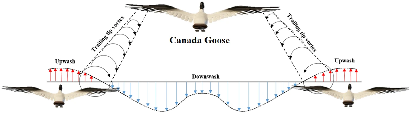
Figure 3: The movement of airflow around a bird.

In this section, we apply the theoretical results above to analyzing the emergence of the line formation of migrating birds. In most of existing researches on this topic, each bird is approximated by a fixed wing, whose forward motion stirs the air around upward and downward. If a bird positions properly relative to another bird, it can get extra lift from the upward airflow generated by that bird and reduce the energy used to counter the gravity, see Fig. 3. This can be regarded as the wake benefit from one bird to another. The movement of the stirred air is usually depicted by a horseshoe vortex model [15], Readers can refer to [15] for more details on the model. We only introduce how to get the wake benefit here.

Assume that two birds $i=0,1$, with the same weight $W$ and wingspan $2b$ (the length of the wing), fly together along the $x$ direction with constant speed $U$, in the plane. If bird $0$ is at the origin $[0\ 0]^{\top}$, the upward airflow velocity $v(x,y)$ at $[x\ y]^{\top}\in\mathbb{R}^{2}$ generated by bird 0 can be given as

$$v(x,y)=v_{b}(x,y)+v_{t}(x,y)$$ (16)

$$v_{b}=\text{\footnotesize{$\frac{\Gamma}{4\pi}\frac{x}{x^{2}+r_{0}^{2}}\left[\frac{y+a}{\sqrt{(y+a)^{2}+x^{2}+r_{0}^{2}}}-\frac{y-a}{\sqrt{(y-a)^{2}+x^{2}+r_{0}^{2}}}\right]$}}$$

$$v_{t}=\text{\footnotesize{$\frac{\Gamma}{4\pi}\frac{y-a}{(y-a)^{2}+R(x)}\left[1-\frac{x}{\sqrt{(y-a)^{2}+x^{2}+R(x)}}\right]$}}$$

$$-\frac{\Gamma}{4\pi}\frac{y+a}{(y+a)^{2}+R(x)}\left[1-\frac{x}{\sqrt{(y+a)^{2}+x^{2}+R(x)}}\right]$$

where $a=\frac{\pi}{4}b$, $\rho$ is the air density, $\Gamma=W/(2\rho aU)$, $R(x)=r_{0}^{2}+D_{f}|x|/U$ with $r_{0}=0.04b$ and $D_{f}$ is a diffusion term to model wake dissipation when $|x|\rightarrow\infty$ [21, 19]. We select $D_{f}=1.05\times 10^{-4}Ub$ such that $\sqrt{R(x)}$ increases from $0.04b$ to $0.1b$ when $|x|$ grows from $0$ to $80b$, fairly realistic for aircraft wake [25]. The model is valid for a sufficiently long longitudinal distance that covers the range of distances of neighboring birds in migratory formation. Beyond that distance, it is not accurate due to wake instability.

Consider bird $1$ locating at $[x\ y]^{\top}$. After neglecting the momentum induced by the vertical airflow as in [15], the wake benefit of bird $1$ received from bird $0$ can be given as

$$f(x,y)=\frac{1}{2b}\int_{y-b}^{y+b}v(x,\eta)\mathrm{d}\eta$$ (17)

This function satisfies Assumption 1 except for the points at the $y$ axis. Computation shows that $f(x,y)$ has a maximum $(-\alpha,-\beta)$ in the negative orthant, with $\alpha\approx 3.468b$ and $\beta\approx(1+\frac{\pi}{4})b=a+b$, Moreover, it peaks around the line $y=-\beta$ in the negative orthant, which is argued [13] to be the best relative lateral position of a follower to its front neighbor. Hence, we fix $\beta$ in all the theorems previously as this value. Fig. 4 shows $f(x,y)$ for $y=-\beta,-2\beta$ when $2b=1.5$. Normally, neighboring birds’ longitudinal distance in migratory formation ranges from 0.5 wingspan ($1b$) to 4 wingspan ($8b$), implying $x_{i(i-1)}\in[-8b,-1b]$ in our setting.

As mentioned before, we have been working on reconstructing the line formation of migrating birds based on the assumption that birds behavior are purely guided by wake benefit maximization, taking into account birds attitudes. We have not numerically found the NE $X^{*}\in\mathbb{R}^{n}$ with $x^{*}_{i(i-1)}\in\mathcal{P}$ and the CE $\bar{X}^{*}\in\mathbb{R}^{n}$ with $\bar{x}^{*}_{i(i-1)}\in\mathcal{P}$ for a much wide interval $\mathcal{P}$, e.g., $[-20b,-b]$ [22]. In the following, we confirm this numerical result.

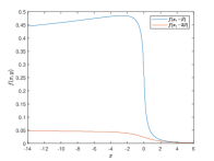
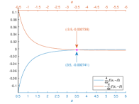
Figure 4: (a) The wake benefit $f(p)$ for $y=-\beta,-2\beta$ when $2b=1.5$ m. (b) The derivative of $f(x,-\beta)$. The point mark and $x$-axis with the same color corresponds to the derivative curve in that color. $\delta_{2}=-0.002741$ and $-\delta_{1}=-0.002738$.

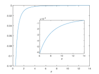
(a) $f_{x}(x,-\beta)$.

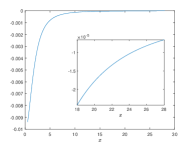
(b) $f_{x}(x,-2\beta)$.

Figure 5: $f_{x}(x,y)$ for positive $x$.

V-A Absence of the NE of interest

We first look at the selfish agents case. An illustrative example is presented for Canadian geese, which averagely have the weight $W=36.75$ N, wingspan $2b=1.5$m, and fly with $U=18$ m/s at the height of $1$km from the ground during migration flight, where the air density $\rho\approx 1.112\text{\ kg}/\text{m}^{3}$. Recall condition (8) and (11), in the following, we always denote $\delta_{1}=\max_{x\in\mathcal{P}}f_{x}(x,-\beta)$, $\delta_{2}=\max_{x\in-\mathcal{P}}f_{x}(x,-\beta)$ and $\delta_{3}=\max_{x\in-\mathcal{Q}(\mathcal{I})}f_{x}(x,-\beta)$ for the corresponding interval $\mathcal{P}$ and $\mathcal{Q}(\mathcal{I})$ accordingly.

By Fig. 4, we can find that if we select $\mathcal{P}=[-\alpha_{l},-\alpha_{s}]=[-3.5,-0.5]$, $\delta_{2}\leq-\delta_{1}$. Hence condition (8) in Theorem 1 holds, and there should exist no NE $X^{*}$ with $x^{*}_{i(i-1)}\in\mathcal{P},i\in V$. Note that $\alpha_{l}$ cannot be increased more as the condition $\delta_{2}<-\delta_{1}$ would not be satisfied.

On the other hand, $f(x,-\beta)$ peaks at $-\alpha=-3.468b=-2.601$ and we can see from Fig. 5(a) and 6 that Assumption 2 is satisfied. Let $\mathcal{P}=[-\alpha_{l},-\alpha_{s}]=[-7,-2.5]\ni-\alpha$, then ${\mathcal{I}}=2\mathcal{P}=[-14,-5]$. The value of $\varepsilon_{\mathcal{I}}$ can be found in Fig. 6. Moreover, the set $\mathcal{Q}(\mathcal{I})=[-\alpha^{\prime}_{l},-\alpha^{\prime}_{s}]$ satisfying (10) is a neighborhood of $-\alpha$ and given as $[-2.78,-2.5]$. Then by Fig. 6, $\delta_{3}\leq-\delta_{1}$ or condition (11) holds. Hence, by Theorem 2, there exists no NE $X^{*}$ with $x^{*}_{i(i-1)}\in\mathcal{P},i\in V$ for $\mathcal{P}=[-7,-2.5]$. The value of $\alpha_{s}$ cannot be much smaller than 2.5, since from Fig. 6, it would imply a wider $\mathcal{I}$, larger $\varepsilon_{\mathcal{I}}$, wider interval $\mathcal{Q}(\mathcal{I})$, and $\delta_{3}$ that would be larger than $-\delta_{1}$, making the condition in Theorem 2 unsatisfied.

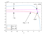
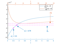
Figure 6: $f_{x}(x,y)$ for $y=-\beta$ and $-2\beta$. The value $\varepsilon_{\mathcal{I}}=\max_{x\in\mathcal{I}}f_{x}(x,-2\beta)$ with ${\mathcal{I}}=2\mathcal{P}=[-14,-5]$ is represented as the dashed magenta lines. The two ends of $\mathcal{Q}(\mathcal{I})$ are $-\alpha^{\prime}_{l}$ and $-\alpha^{\prime}_{s}$.

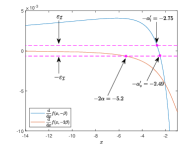
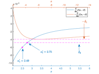
Figure 7: $f_{x}(x,y)$ for $y=-\beta$ and $-2\beta$. The value $\varepsilon_{\mathcal{I}}$ with $\mathcal{I}=[-2\alpha_{l},-2\alpha]=[-28,-5.2]$ is represented as the dashed magenta lines. The two ends of $\mathcal{Q}(\mathcal{I})$ are $-\alpha^{\prime}_{l}$ and $-\alpha^{\prime}_{s}$.

Note as mentioned before this subsection, no NE $X^{*}$ of interest has been found for a wide $\mathcal{P}$, e.g., $[-20b,-b]=[-15,-0.75]$. Hence, the two previous paragraphs are not able to explain this. We then turn to Theorem 3. By Fig. 5(b) and 7, Assumption 3 is indeed satisfied for $x\geq-2\alpha$ (The curve of $f_{x}(x,-2\beta)<0$ for $x\leq-14$ is not shown for a clear vision of $\varepsilon_{\mathcal{I}}$). Let $\mathcal{P}=[-14,-0.5]\ni-\alpha$, then $\mathcal{I}=[-28,-1]$. In Fig. 7, we can find $\mathcal{Q}(\mathcal{I})=[-\alpha^{\prime}_{l},-\alpha^{\prime}_{s}]$ that satisfies (10). Then by Fig. 7, $\delta_{3}<-\delta_{1}$. Hence conditions (11) in Theorem 3 holds for $\mathcal{P}=[-14,-0.5]$, from which, we should have that there exists no NE $X^{*}$ of interest for this interval. This indeed explains our numerical search of the NE of interest.

V-B Absence the CE of interest

We then show that there exists no CE $\bar{X}^{*}$ of interest for a negative closed interval $\mathcal{P}$ with the wake benefit function (17). For this function, we have following result.

Lemma 1

The benefit $f(x,y)$ in (17) satisfies condition (14) with $\alpha_{l}\leq\frac{U}{D_{f}}(2ab-r_{0}^{2}),\underline{\beta}\in(\sqrt{a^{2}+b^{2}},\beta)$.

The proof of this result is given in Appendix. Accordingly, we have the following result.

Proposition 4

Consider the function $f(x,y)$ in (17) and $n\geq 2$, then there exists no CE $\bar{X}^{*}\in\mathbb{R}^{n}$ such that $\bar{x}_{i(i-1)}^{*}\in\mathcal{P}$ for any $\mathcal{P}=[-\alpha_{l},-\alpha_{s}]$ with $0<\alpha_{s}\leq\alpha_{l}\leq\frac{U}{D_{f}}(2ab-r_{0}^{2})$.

Proof. By Lemma 1, we have that condition (14) is satisfied with $\underline{\beta}\in(\sqrt{a^{2}+b^{2}},\beta)$ and $\alpha_{l}\leq\frac{U}{D_{f}}(2ab-r_{0}^{2})$. This combining with Theorem 4 shows that for any $\mathcal{P}=[-\alpha_{l},-\alpha_{s}]$ with $0<\alpha_{s}\leq\alpha_{l}\leq\frac{U}{D_{f}}(2ab-r_{0}^{2})$, there exists no CE of interest.  $\blacksquare$

Putting $D_{f}=1.05\times 10^{-4}Ub$, $a=\frac{\pi}{4}b$ and $r_{0}=0.04b$ into $\frac{U}{D_{f}}(2ab-r_{0}^{2})$ yields $\alpha_{l}\leq 14945b$ or $7472$ wingspan. Based on the employed wake benefit model (17), the proposition predicts that no CE $\bar{X}^{*}$ of interest for an closed interval $\mathcal{P}\subset[-14945b,0)$ exists. Hence the echelon formation where each neighboring birds have the lateral distance of $(\frac{1}{2}+\frac{\pi}{8})$ wingspan and longitudinal distances less than $7472$ wingspans cannot emerge, when birds are cooperative to maximize the total wake benefit of the flock. It should be noticed that echelon formation with the longitudinal distance of neighboring birds larger than $7472$ wingspans is not practical, as birds never fly so far from each other in formation flight. Furthermore, the fixed wing wake model may not be valid for such large longitudinal distance.

VI Conclusion

In this paper, we focus the two-dimensional echelon formation of multi-agents that behave to maximize relative-position dependent benefits. All the agents can be either selfish to maximize its own benefit from others or cooperative to optimize the total benefit of the group. We discuss the conditions on the inter-agent benefit such that echelon formations cannot appear, no matter agents are selfish or cooperative. The theoretical conditions are employed to analyze the fixed-wing model that is usually used to study line formations of migrating birds, and justify our failure in numerically reconstructing migratory formations. This shows that the emergence of this kind formation may not emerge if birds behavior in migration is purely guided by energy savings.

Our results imply multiple possibilities for the emergence reason of the migratory formations. First, remember that we employ the fixed-wings to model birds and ignore the slow undulatory motion of birds wings, conventionally as in [13, 14], a natural hypothesis is that the wing-flapping of birds plays more important roles than expected. Nevertheless, fixed-wings are proper to represent the glide of birds in formation flight. Hence, a second hypothesis from our result is that non-aerodynamic factors, such as collision avoidance and vision enhancement [13] could also take parts in developing the migratory formation. Finally, from the perspective of multi-agent control systems, more complex dynamics, the actual sensing and information processing ability of the bird, and the communication capacity among birds (for cooperative birds) may need to be considered to see if the current result would still hold.

Appendix: Proof of Lemma 1

By (16) and (17), we have

$$f(p)=\frac{1}{2b}\int_{y-b}^{y+b}v_{b}(x,\eta)\mathrm{d}\eta+\frac{1}{2b}\int_{y-b}^{y+b}v_{t}(x,\eta)\mathrm{d}\eta$$

For the two integration in the equation above, we can obtain

$$\frac{1}{2b}\int_{y-b}^{y+b}v_{b}(x,\eta)\mathrm{d}\eta$$

$$= \frac{\Gamma}{8\pi b}\frac{x}{x^{2}+r_{0}^{2}}\left.\left[\sqrt{(\eta+a)^{2}+x^{2}+r_{0}^{2}}-\sqrt{(\eta-a)^{2}+x^{2}+r_{0}^{2}}\right]\right|^{y+b}_{y-b}$$

$$= \frac{\Gamma}{8\pi b}\frac{x}{x^{2}+r_{0}^{2}}\left[\sqrt{c_{3}+x^{2}+r_{0}^{2}}-\sqrt{(c_{2}+x^{2}+r_{0}^{2}}\right.$$

$$~{}~{}~{}~{}~{}~{}~{}~{}~{}~{}~{}~{}~{}~{}~{}~{}\left.-\sqrt{c_{1}+x^{2}+r_{0}^{2}}+\sqrt{c_{4}+x^{2}+r_{0}^{2}}\right]$$ (18)

$$\frac{1}{2b}\int_{y-b}^{y+b}v_{t}(x,\eta)\mathrm{d}\eta$$

$$= \frac{\Gamma}{8\pi b}\left[\ln\sqrt{(\eta-a)^{2}+R}-\frac{1}{2}\ln\left(\frac{\sqrt{(\eta-a)^{2}+x^{2}+R}-x}{\sqrt{(\eta-a)^{2}+x^{2}+R}+x}\right)\right.$$

$$\left.\left.-\sqrt{(\eta+a)^{2}+R}-\frac{1}{2}\ln\left(\frac{\sqrt{(\eta+a)^{2}+x^{2}+R}-x}{\sqrt{(\eta+a)^{2}+x^{2}+R}+x}\right)\right]\right|_{y-b}^{y+b}$$

$$= \frac{\Gamma}{8\pi b}f_{t1}(x,y)+\frac{\Gamma}{16\pi b}f_{t2}(x,y)$$ (19)

where

$$c_{1}= (y+b-a)^{2},\quad c_{2}=(y-b+a)^{2}$$

$$c_{3}= (y+b+a)^{2},\quad c_{4}=(y-b-a)^{2}$$

$$f_{t_{1}}(x,y)= \frac{1}{2}\ln\frac{(c_{1}+R)(c_{2}+R)}{(c_{3}+R)(c_{4}+R)}$$

$$f_{t_{2}}(x,y)= \ln\left(\frac{\sqrt{c_{3}+x^{2}+R}-x}{\sqrt{c_{3}+x^{2}+R}+x}\right)+\ln\left(\frac{\sqrt{c_{4}+x^{2}+R}-x}{\sqrt{c_{4}+x^{2}+R}+x}\right)$$

$$-\ln\left(\frac{\sqrt{c_{1}+x^{2}+R}-x}{\sqrt{c_{1}+x^{2}+R}+x}\right)-\ln\left(\frac{\sqrt{c_{2}+x^{2}+R}-x}{\sqrt{c_{2}+x^{2}+R}+x}\right)$$

It should be notified that $c_{1},c_{2},c_{3}$, and $c_{4}$ depend on $y$. By equation (18) and (19), one can check that

$$\frac{1}{2b}\int_{y-b}^{y+b}v_{b}(x,\eta)\mathrm{d}\eta+\frac{1}{2b}\int_{-y-b}^{-y+b}v_{b}(-x,\eta)\mathrm{d}\eta=0,$$

$$f_{t1}(x,y)+f_{t1}(-x,-y)=\ln\frac{(c_{1}+R)(c_{2}+R)}{(c_{3}+R)(c_{4}+R)},$$ (20)

$$f_{t2}(x,y)+f(-x,-y)=0.$$

Then

$$f(x,y)+f(-x,-y)$$

$$= \frac{1}{2b}\int_{y-b}^{y+b}v_{b}(x,\eta)\mathrm{d}\eta+\frac{1}{2b}\int_{y-b}^{y+b}v_{t}(x,\eta)\mathrm{d}\eta$$

$$+\frac{1}{2b}\int_{-y-b}^{-y+b}v_{b}(-x,\eta)\mathrm{d}\eta+\frac{1}{2b}\int_{-y-b}^{-y+b}v_{t}(-x,\eta)\mathrm{d}\eta$$

$$= \frac{1}{2b}\int_{y-b}^{y+b}v_{t}(x,\eta)\mathrm{d}\eta+\frac{1}{2b}\int_{-y-b}^{-y+b}v_{t}(-x,\eta)\mathrm{d}\eta$$

$$= \frac{\Gamma}{8\pi b}(f_{t1}(x,y)+f_{t1}(-x,-y))$$

$$+\frac{\Gamma}{16\pi b}(f_{t2}(x,y)+f_{t2}(-x,-y))$$

$$= \frac{\Gamma}{8\pi b}(f_{t1}(x,y)+f_{t1}(-x,-y))$$

which according to (20) is a function of $R$. Recall that $R(x)=r_{0}^{2}+\frac{D_{f}}{U}|x|=r_{0}^{2}+\frac{D_{f}}{U}x$ when $x\geq 0$, we have

$$\frac{\partial}{\partial x}(f(x,y)+f(-x,-y))$$

$$= \frac{\Gamma}{8\pi b}\frac{\partial}{\partial R}\left(f_{t1}(x,y)+f_{t1}(-x,-y)\right)\frac{\text{d}R}{\text{d}x}$$

$$= \frac{\Gamma}{8\pi b}\frac{\text{d}R}{\text{d}x}\frac{\partial}{\partial R}\ln\frac{(c_{1}+R)(c_{2}+R)}{(c_{3}+R)(c_{4}+R)}$$

$$= \frac{\Gamma}{8\pi b}\frac{\text{d}R}{\text{d}x}\frac{g(R)}{(c_{1}+R)(c_{2}+R)(c_{3}+R)(c_{4}+R)},$$ (21)

where

$$g(R)= (2R+c_{1}+c_{2})(c_{3}+R)(c_{4}+R)$$

$$-(2R+c_{3}+c_{4})(c_{1}+R)(c_{2}+R)$$

$$= 8ab(R^{2}+c_{6}R+c_{7})$$

with $c_{6}=2(a^{2}+b^{2}-y^{2})$ and $c_{7}=-3y^{4}+2(a^{2}+b^{2})y^{2}+(a^{2}-b^{2})^{2}$.

Note that when $x>0$, $\frac{dR(x)}{dx}>0$, $R(x)>0$, and the denominator under $g(R)$ in (Appendix: Proof of Lemma 1) is always positive, hence the sign of (Appendix: Proof of Lemma 1) is the same as that of $g(R)$. In order to check if there exists some positive $\underline{\beta}\leq\beta$ such that condition (14) holds for the $\alpha_{l}$ satisfying the condition in the lemma, we test that if there exists this $\underline{\beta}$ such that for any $y$, with $|y|\in[\underline{\beta},+\infty)$, the quadratic inequality $g(R)<0$ holds when $R\in(r_{0}^{2},r_{0}^{2}+\frac{D_{f}\alpha_{l}}{U}]$. It is easy to know that if $|y|\geq\sqrt{a^{2}+b^{2}}$, $c_{6},c_{7}<0$ and $g(R)<0$ hold when

$$R\in (0,\frac{-c_{6}+\sqrt{c_{6}^{2}-4c_{7}}}{2})$$

$$=(0,y^{2}-(a^{2}+b^{2})+2\sqrt{(y^{2}-a^{2})(y^{2}-b^{2})})$$ (22)

The right open end of this interval is an increasing function of $y^{2}$ when $|y|\geq\sqrt{a^{2}+b^{2}}$ and equals to $2ab$ when $|y|=\sqrt{a^{2}+b^{2}}$. Note that $\beta=a+b>\sqrt{a^{2}+b^{2}}$, if we take $\underline{\beta}\in(\sqrt{a^{2}+b^{2}},\beta)$, the intersection of the interval (22) for all $|y|\in[\underline{\beta},+\infty)\subset[\sqrt{a^{2}+b^{2}},+\infty)$ is $(0,2ab+o)$ for some $o>0$. Hence, $g(R)<0$ holds for any $R\in(0,2ab]$ when $|y|\in[\underline{\beta},+\infty)$.

Recall $r_{0}^{2}=(0.02b)^{2}$ and $a=\frac{\pi}{4}b$, we have $2ab>r_{0}^{2}$ and for any positive $\alpha_{l}\leq\frac{U}{D_{f}}(2ab-r_{0}^{2})$, $(r_{0}^{2},r_{0}^{2}+\frac{D_{f}}{U}\alpha_{l}]\subset(0,2ab]$. This shows that when $|y|\in[\underline{\beta},+\infty)$, for any $R\in(r_{0}^{2},r_{0}^{2}+\frac{D_{f}}{U}\alpha_{l}]$ with $0<\alpha_{l}\leq\frac{U}{D_{f}}(2ab-r_{0}^{2})$, $g(R)<0$ holds. In other words, condition (14) holds for $\alpha_{l}\leq\frac{U}{D_{f}}(2ab-r_{0}^{2})$, $\underline{\beta}\in(\sqrt{a^{2}+b^{2}},\beta)$.  $\blacksquare$

References

- [1] K.-K. Oh, M.-C. Park, and H.-S. Ahn, “A survey of multi-agent formation control,” Automatica, vol. 53, pp. 424–440, 2015.
- [2] W. Dong and J. A. Farrell, “Cooperative control of multiple nonholonomic mobile agents,” IEEE Transactions on Automatic Control, vol. 53, no. 6, pp. 1434–1448, 2008.
- [3] W. Ren and E. Atkins, “Distributed multi-vehicle coordinated control via local information exchange,” International Journal of Robust and Nonlinear Control: IFAC-Affiliated Journal, vol. 17, no. 10-11, pp. 1002–1033, 2007.
- [4] B. D. Anderson, C. Yu, B. Fidan, and J. M. Hendrickx, “Rigid graph control architectures for autonomous formations,” IEEE Control Systems Magazine, vol. 28, no. 6, pp. 48–63, 2008.
- [5] J. M. Hendrickx, B. D. Anderson, J.-C. Delvenne, and V. D. Blondel, “Directed graphs for the analysis of rigidity and persistence in autonomous agent systems,” International Journal of Robust and Nonlinear Control: IFAC-Affiliated Journal, vol. 17, no. 10-11, pp. 960–981, 2007.
- [6] S. Zhao and D. Zelazo, “Bearing rigidity and almost global bearing-only formation stabilization,” IEEE Transactions on Automatic Control, vol. 61, no. 5, pp. 1255–1268, 2015.
- [7] L. Chen, M. Cao, and C. Li, “Angle rigidity and its usage to stabilize multi-agent formations in 2d,” IEEE Transactions on Automatic Control, 2020.
- [8] C. W. Reynolds, “Flocks, herds and schools: A distributed behavioral model,” in Proceedings of the 14th annual conference on Computer graphics and interactive techniques, 1987, pp. 25–34.
- [9] T. Vicsek, A. Czirók, E. Ben-Jacob, I. Cohen, and O. Shochet, “Novel type of phase transition in a system of self-driven particles,” Physical review letters, vol. 75, no. 6, p. 1226, 1995.
- [10] R. Olfati-Saber, “Flocking for multi-agent dynamic systems: Algorithms and theory,” IEEE Transactions on automatic control, vol. 51, no. 3, pp. 401–420, 2006.
- [11] H. G. Tanner, A. Jadbabaie, and G. J. Pappas, “Flocking in fixed and switching networks,” IEEE Transactions on Automatic control, vol. 52, no. 5, pp. 863–868, 2007.
- [12] H. Trenchard and M. Perc, “Energy saving mechanisms, collective behavior and the variation range hypothesis in biological systems: a review,” BioSystems, vol. 147, pp. 40–66, 2016.
- [13] I. L. Bajec and F. H. Heppner, “Organized flight in birds,” Animal Behaviour, vol. 78, no. 4, pp. 777 – 789, 2009.
- [14] H. Weimerskirch, J. Martin, Y. Clerquin, P. Alexandre, and S. Jiraskova, “Energy saving in flight formation,” Nature, vol. 413, no. 6857, pp. 697–698, 2001.
- [15] D. Hummel, “Aerodynamic aspects of formation flight in birds,” Journal of theoretical biology, vol. 104, no. 3, pp. 321–347, 1983.
- [16] J. P. Badgerow and F. R. Hainsworth, “Energy savings through formation flight? a re-examination of the vee formation,” Journal of Theoretical Biology, vol. 93, no. 1, pp. 41–52, 1981.
- [17] D. Hummel, “Formation flight as an energy-saving mechanism,” Israel Journal of Ecology and Evolution, vol. 41, no. 3, pp. 261–278, 1995.
- [18] C. Cutts and J. Speakman, “Energy savings in formation flight of pink-footed geese,” Journal of experimental biology, vol. 189, no. 1, pp. 251–261, 1994.
- [19] F. S. Cattivelli and A. H. Sayed, “Modeling bird flight formations using diffusion adaptation,” IEEE Transactions on Signal Processing, vol. 59, no. 5, pp. 2038–2051, 2011.
- [20] X. Li, Y. Tan, J. Fu, and I. Mareels, “On V-shaped flight formation of bird flocks with visual communication constraints,” in 13th IEEE International Conference on Control & Automation (ICCA). IEEE, 2017, pp. 513–518.
- [21] G. C. Greene, “An approximate model of vortex decay in the atmosphere,” Journal of Aircraft, vol. 23, no. 7, pp. 566–573, 1986.
- [22] M. Shi and J. M. Hendrickx, “Whose energy cost would birds like to save: a revisit of the migratory formation flight,” In preparation.
- [23] T. Başar and G. J. Olsder, Dynamic noncooperative game theory. SIAM, 1998.
- [24] J. B. Rosen, “Existence and uniqueness of equilibrium points for concave n-person games,” Econometrica: Journal of the Econometric Society, pp. 520–534, 1965.
- [25] I. De Visscher, L. Bricteux, and G. Winckelmans, “Aircraft vortices in stably stratified and weakly turbulent atmospheres: Simulation and modeling,” AIAA journal, vol. 51, no. 3, pp. 551–566, 2013.