Interplay between transport and quantum coherences in free fermionic systems

Abstract

We study the quench dynamics in free fermionic systems in the prototypical bipartitioning protocol obtained by joining two semi-infinite subsystems prepared in different states, aiming at understanding the interplay between quantum coherences in space in the initial state and transport properties. Our findings reveal that, under reasonable assumptions, the more correlated the initial state, the slower the transport is. Such statement is first discussed at qualitative level, and then made quantitative by introducing proper measures of correlations and transport “speed”. Moreover, it is supported for fermions on a lattice by an exact solution starting from specific initial conditions, and in the continuous case by the explicit solution for a wider class of physically relevant initial states. In particular, for this class of states, we identify a function, that we dub transition map, which takes the value of the stationary current as input and gives the value of correlation as output, in a protocol-independent way. As an aside technical result, in the discrete case, we give an expression of the full counting statistics in terms of a continuous kernel for a general correlated domain wall initial state, thus extending the recent results in [Moriya, Nagao and Sasamoto, JSTAT 2019(6):063105] on the one-dimensional XX spin chain.

1 Introduction

How does quantum coherence affect a quantum many-body system far from equilibrium? Answering such a question not only enhances our understanding of the nature of dynamics in quantum systems, but also helps us design quantum materials with desired dynamical properties at will, something which is feasible today thanks to the unprecedented control in manipulating such systems [1, 2, 3, 4]. Indeed, while initially quantum states in experiments have been prepared in either the ground state or in a thermal state of the system, today it is possible to engineer novel exotic states with peculiar coherent properties (e.g., quantum simulations [5, 6, 7], fragmented Bose-Einstein condensates [8, 9]). Such experimental realizations of correlated initial states in unconventional ways therefore call for a theoretical understanding of the effect of initial correlations on the subsequent dynamics.

Amongst possible situations where such attempts can be made, in the present work we focus on transport phenomena in one-dimensional systems. The simple situation we have in mind is the extensively studied bipartitioning protocol [10, 11, 12, 13, 14, 15, 16, 17, 18], where two semi-infinite systems are prepared in different states and then joined together. An “imbalance” between them will generate a flow from one side to another. In particular, we ask the following question: Does the presence of initial spatial correlations have an effect on transport in quench protocols?

For generic systems, hydrodynamic serves as a convenient tool to study transport problems, which has the advantage to be accessible also in presence of interactions. Hydrodynamics has been successfully applied to numerous systems, ranging from quark-gluon plasma [19] to graphene [20], and more recently, to quantum integrable systems [21, 22]. In the latter context, it was termed generalized hydrodynamics (GHD), and has proved to be a powerful tool in characterizing the large-scale dynamics of integrable systems with a great analytic handle [21, 22, 23, 24, 25]. Importantly, its validity has been confirmed in recent experiments [26, 27].

However, it is not clear whether this approach can give a complete answer to our question. In fact, this theory is in general unable to capture effects due to correlations which are very far apart. One of its underlying assumptions, indeed, is that of local equilibration within fluid cells, which means that different fluid cells are completely uncorrelated in this approximation, thus eventually leading to a partial loss of information with respect to the exact initial problem [28]. We mention, however, that there has been some (partially successful) attempts to extend GHD so to include such long-range correlations [29, 30, 31, 32].

This motivates us to take a step back and consider the simplest example of integrable system, namely one-dimensional free fermions, for which numerous aspects can be studied analytically by means of exact calculations.

More specifically, we will consider the bipartite situation where the right ($\mathcal{R}$) side is initially empty, while the left ($\cal{L}$) side is prepared in a given state at the fixed value of the average density $n_{0}$. We will study how the flow is affected when one varies the typical length-scale over which particles in the $\cal{L}$-side are correlated (i.e., the coherence length), as depicted in Fig 1. Under physically plausible assumptions (that we are going to detail below, cf. Section 3.2), we observe a clear phenomenon: the more correlated the state, the slower the transport. To establish this statement at quantitative level, we shall introduce two quantities that measure the speed of (mass) transport and the strength of correlation, which will enable us to talk about these two different notions on an equal footing (Section 3.4).

Interestingly, this phenomenon is strongly linked to the integrable nature of the system, namely the existence of an infinite number of conserved quantities. A clear way to see that is the following. In the bipartition protocol, if we take two initial states with the same particle, momentum and energy densities, then conventional hydrodynamics [28] (meaning for systems with few conservation laws, as opposite to the “generalized” one for integrable models [33]) will predict the same flow for the two of them. However, for integrable models there may be an imbalance in the infinitely many other conserved charges of the system, giving rise to different currents  [33]. As a striking illustration, it would be for instance possible to engineer two protocols I and II where the particle, momentum and energy densities are all higher in protocol I but the flow would still be greater in protocol II. This interplay between the flow of different conserved charges is another interesting observation of our analysis, and can be thought of as an analogue of the famous thermoelectric effect [34] for integrable systems.

Finally, in relation to the initial issue of the limits of an hydrodynamic approach when describing long range correlations, this study further clarifies within the specific problem under investigation that, in the free case in continuous space at least, GHD can be though of as an exact theory, rather then an approximation (in particular, no average over fluid cell is needed). In fact our calculations are done in phase-space, relying on the so-called Wigner function [35, 36, 37] in its many-body version [38, 39, 40, 41, 42, 43] (see Section 3 for proper definitions), something which has been known and widely used [44]. On the other hand, in the free limit one can explicitly check that the GHD equation simply reduces to the (continuous) evolution equation for the aforementioned Wigner function. And since the latter can be derived without any further assumptions, the two approaches turn out to be equivalent, and, importantly, both exact. This exact viewpoint of GHD is taken in Ref. [29, 30] for lattice free fermions, to derive the corrections due to the lattice in the form of Moyal expansion [45]. Further study is, instead, needed to understand the role of the hydrodynamic approximation (in particular, of fluid cells) in the interacting case. Some of the complications which occur in the attempt of extending our results in this direction are mentioned towards the end of the paper (Section 4), but the general issue is left to future investigation.

Let us close this introduction by putting our specific quench problem in some more context within the existing literature on transport and correlations in free fermion, where in fact a great deal of analytic studies has been done in the past. Apart the standard references on bipartitioning protocols mentioned above, full counting statistics and large deviation in free fermionic systems have also been intensively studied [46, 47, 48, 49, 50, 51, 52]. The effect of quantum correlations in stochastic, diffusive free fermionic systems was investigated in quantum exclusion processes as well [53, 54, 55, 56]. The entanglement dynamics was considered both in homogeneous [57] and inhomogeneous [58] settings (and, remarkably, extended to interacting integrable models [59, 60, 61, 62, 63, 64]). More recently, the effect of continuous monitoring on the dynamics of a free fermionic chain was studied in [65, 66]. Finally, transport properties in open free fermionic systems have been considered in [67, 68, 69, 70].

Outline.

The paper is structured as follows. We start in Section 2 by considering a specific example of bipartite protocol for free fermions on a lattice. Through exact lattice calculation, we show explicitly that our main claim relating correlations and transport holds. An aside result of this Section is reported in Appendix B, specifically Eq. (73), that expresses the full counting statistics in terms of a continuous kernel for a general correlated domain wall initial state, thus extending the recent results in [50] on the one-dimensional XX spin chain. In Section 3, we move to free fermions in the continuum where a great deal of simplifications occur. We can then consider a large family of initial states for which our statement still holds and, importantly, we manage to make it quantitative by introducing two quantities that measure the speed of (mass) transport and the strength of correlation, and further showing the existence of a transition map which relate them in a protocol-independent way. Finally, we comment on the more involved interacting case in Section 4, and conclude by some perspectives and remarks in Section 5. Some derivations and technical details are reported in the remaining appendices. In particular, the full counting statistics for the half-filled protocol in the discrete case for arbitrary correlated initial conditions is presented there.

Figure 1: Left: Initial state in the bipartitioning protocol where the left-half of the space is filled by particles with occupation $n_{0}$ and the right-half is empty. The top and bottom state are prepared in the same initial state but with different spatial correlation length. Right: Density profile after letting the system evolve for a time $t$. We will show that the more correlated the initial state, the greater the flow is at later times.

2 An exact solution in the discrete case

We begin our investigation by studying a bipartitioning protocol in a free fermionic infinite one-dimensional lattice. In order to exemplify the relation between initial coherences and transport, we will consider a particular correlated domain-wall (to be defined below), where the space is half-filled with fermions, tailored to have quantum coherence up to typical distance $\ell_{c}$, and study the effect on particles transport when varying $\ell_{c}$.

The study of the uncorrelated domain-wall quench in the one-dimensional Heisenberg XX spin chain, equivalent to the free fermions on a lattice through a Jordan-Wigner transformation, has been the subject of many recent studies [10, 48, 50]. These works focus, as we do, on a half-filled initial state, but with no coherence, corresponding to $\ell_{c}=1$ in our notation.

As an aside remark, we mention that while in the rest of the paper we will focus on the average particle number to characterize transport properties of the system, this is in general not sufficient for a full characterization. Instead, much more information can be extracted from higher momenta, all contained in the full counting statistics (FCS). While the latter is more difficult to study analytically, a result in this direction is reported in Appendix B, where we derive a Fredholm determinant representation of the FCS, when starting from an arbitrary initial state with support on half of an infinite chain. This result extends the work [50] of Moriya, Nagao and Sasamoto, which was restricted to the uncorrelated case, to a generally correlated initial condition.

2.1 The model and setup

The model under consideration is defined by the following Hamiltonian

$$\hat{H}=-\frac{1}{2}\sum_{m=-\infty}^{\infty}\big{(}c_{m}^{\dagger}c_{m+1}+c_{m+1}^{\dagger}c_{m}\big{)}$$ (1)

where the creation and annihilation operators obey the fermionic algebra

$$\{c_{n}^{\dagger},c_{m}^{\dagger}\}=\{c_{n},c_{m}\}=0,\qquad\{c_{n},c_{m}^{\dagger}\}=\delta_{nm},\qquad c_{n}^{2}=(c_{n}^{\dagger})^{2}=0,$$ (2)

with the anti-commutator defined by $\{A,B\}=AB+BA$. $\hat{H}$ can be diagonalized in Fourier space, with the fermionic momentum operators $\tilde{c}_{k}=\sum_{j=-\infty}^{\infty}e^{-\mathbf{i}jk}c_{j}$, and the single-particle spectrum reads $\{-\cos(k)\}_{k\in[-\pi,\pi]}$.

We proceed by defining the time-dependent correlation matrix $\hat{C}(t)$ with matrix elements

$${C}_{mn}(t)=\langle c_{m}^{\dagger}(t)c_{n}(t)\rangle$$ (3)

where $c_{n}(t)$ denote the time-evolved fermionic operators. Standard calculations lead to the explicit and general expression

$$\hat{C}(t)=\hat{J}(t)^{\dagger}{\hat{C}}_{0}\hat{J}(t)\;.$$ (4)

where $\hat{C}_{0}=\hat{C}(t=0)$ (which contains the information about the initial state) and $\hat{J}(t)$ has matrix elements ${J}_{mn}(t)=\mathbf{i}^{m-n}J_{m-n}(t)$ in terms of the $(m-n)^{\mathrm{th}}$ Bessel function of the first kind $J_{m-n}(t)$ [71].

2.2 A particular correlated domain-wall state

We now specialize to a particular initial state. To this aim, we divide the lattice in two halves ${\cal L}\mathrel{\mathop{\mathchar 58\relax}}=\mathbb{Z}^{-}\cup\{0\}$ and ${\cal R}\mathrel{\mathop{\mathchar 58\relax}}=\mathbb{Z}^{+}$. The $\cal{R}$-side is empty of particles, while the $\cal{L}$-side has fixed density $n_{0}$ and coherence length $\ell_{c}$, which is obtained by taking $n_{0}\ell_{c}$ particles living on $\ell_{c}$ sites as follows.

First, for a given unit cell of $\ell_{c}$ sites, consider the so-called Dicke state [72, 73]

$$\ket{\phi^{\ell_{c}}_{n_{0}\ell_{c}}}=\frac{1}{\sqrt{\binom{\ell_{c}}{n_{0}\ell_{c}}}}\sum_{{\cal C}(n_{0},\ell_{c})}\ket{{\cal C}}$$ (5)

where ${\cal C}(n_{0},\ell_{c})$ indexes all the possible ways of arranging $n_{0}\ell_{c}$ particles. This can be formulated as ${\cal C}(n_{0},\ell_{c})$ being a binary vector in $\{0,1\}^{\ell_{c}}$ with $n_{0}\ell_{c}$ elements equal to $1$. For instance, for $n_{0}\ell_{c}=2$ and $\ell_{c}=4$ :

$$\ket{\phi^{\ell_{c}}}=\frac{1}{\sqrt{6}}\big{(}\ket{\bullet\bullet\circ\circ}+\ket{\bullet\circ\bullet\circ}+\ket{\bullet\circ\circ\bullet}+\ket{\circ\bullet\bullet\circ}+\ket{\circ\bullet\circ\bullet}+\ket{\circ\circ\bullet\bullet}\big{)}.$$

Figure 2: The initial state we consider in Section 2. Panel (a): Cartoon picture of the state. The lattice is half-filled with particle with mean density $n_{0}$ in the left-side ($\mathcal{L}$), while it is empty in the right-side ($\mathcal{R}$). In $\mathcal{L}$, particles are correlated on a typical distance $\ell_{c}$ that we call the quantum coherence length. Panel (b): Total two-point correlation function $\hat{C}_{0}^{\mathcal{L}}$ (right), and its restriction to the $\mathcal{L}$ sector, $\hat{C}_{0}^{\mathcal{L}}$, where matrix elements (given in (7)) decay to $0$ on a typical distance given by $\ell_{c}$. Previous studies assumed $\hat{C}_{0}^{\mathcal{L}}$ to be completely diagonal.

Then, if $\varrho^{\ell_{c}}\mathrel{\mathop{\mathchar 58\relax}}=\ket{\phi^{\ell_{c}}_{n_{0}\ell_{c}}}\bra{\phi^{\ell_{c}}_{n_{0}\ell_{c}}}$ is the associated density matrix, the total density matrix in the $\cal{L}$-side is taken as

$$\varrho_{{\rm tot}}=\frac{1}{\ell_{c}}\sum_{j=-(\ell_{c}-1)}^{0}\cdots\otimes\varrho_{[-(2\ell_{c}-1+j),-(\ell_{c}+j)]}^{\ell_{c}}\otimes\varrho_{[-(\ell_{c}-1+j),j]}^{\ell_{c}}$$ (6)

where the brakets $[,]$ indicate the support of the density matrix.

The calculation of the corresponding two-point correlation function $\hat{C}^{\rm tot}$ is straightforward, and its matrix elements read

$$C^{\rm tot}_{m,n}=\begin{cases}n_{0}&\text{for }m=n\text{ and}\\ \frac{(\ell_{c}-|m-n|)}{\ell_{c}}\times c_{1,1+|m-n|}^{\ell_{c}}&\text{for }m\neq n\text{ and }|m-n|\leqslant\ell_{c}\\ 0&\text{otherwise}\end{cases}$$ (7)

in terms of $c_{j,k}^{\ell_{c}}={{\rm Tr}}(\varrho^{\ell_{c}}c_{j}^{\dagger}c_{k})$, namely the two-point correlation within a coherent cell. Evaluating $c_{j,k}^{\ell_{c}}$ can be a tedious task because of the fermionic anti-commutation relations. This is nevertheless done, for completeness, in Appendix A.1 for the general case. Here, instead, for simplicity, we restrict to the case where there is one particle in a given cell, i.e., $n_{0}={1}/{\ell_{c}}$, giving $c_{j,k}^{\ell_{c}}={1}/{\ell_{c}}$ for all $(j,k)$ in $[1,\ell_{c}]\times[1,\ell_{c}]$. [For comparison, the uncorrelated domain-wall studied in [10, 48, 50] is instead represented by an initial diagonal correlation matrix with matrix elements $C_{m,n}^{{\cal D}}=n_{0}\delta_{m,n}$. Note that the two situations cannot be distinguished by only probing on-site observables.]

Finally, the total two point function is then $\hat{C}_{0}=\hat{C}_{0}^{\mathcal{L}}\oplus\hat{C}_{0}^{\mathcal{R}}$, with $\hat{C}^{\mathcal{R}}_{0}=\hat{C}^{\rm tot}$ and $\hat{C}^{\mathcal{R}}_{0}=0$, as shown in Fig. 2. Such initial condition together with Eq. (4), gives the local density $C_{m,m}(t)$ at site $m$ as (see Appendix A.2 for details).

$$C_{m,m}(t) =n_{0}B_{t}(m,m)+2\sum_{k=1}^{\ell_{c}}\cos(\frac{k\pi}{2})C_{k}B_{t}(m+k,m)$$ (8)

where $B_{t}(m,n)$ is the discrete Bessel kernel (cf. Eq. (57) in Appendix A.2) and $C_{j_{1}-j_{2}}\mathrel{\mathop{\mathchar 58\relax}}=(\hat{\mathcal{C}}_{0}^{\mathcal{L}})_{j_{1},j_{2}}(t=0)$. We define the hydrodynamic limit $\lim_{\rm{h}}$ by the limit where $t\to\infty$, $m\to\infty$ while $u\mathrel{\mathop{\mathchar 58\relax}}=\frac{m}{t}$ is kept fixed. Let $\Phi(u)=\lim_{\rm{h}}C_{m,m}(t)$, we then have (see Appendix A.3 for the proof)

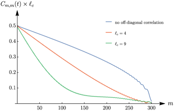
Figure 3: Density profile at $t=300$ in the right half-space for difference coherence length. For readability, all the curves have been rescaled by a factor $\ell_{c}$ to match at the origin.

$$\Phi(u)=\frac{\arccos(u)}{\pi\ell_{c}}+\frac{2}{\pi}\sum_{k=1}^{\ell_{c}}\cos\left(\frac{k\pi}{2}\right)\frac{\ell_{c}-k}{k\ell_{c}^{2}}\sin(k\arccos(u))$$ (9)

In Fig. 3 we plotted for fixed time $t=300$ the density profile in the $\cal{R}$-part of the system, for different choice of $\ell_{c}$. For readability, all the curves are rescaled so that they match at the origin. We clearly see that the transport is affected by the coherence present in the initial state. Specifically, that the more correlated the state, the slower is the transport.

From the local density, one can further obtain the total number of particle in ${\cal R}$ at time $t$ as

$$\mathcal{N}_{{\cal R}}(t)=\sum_{m\in\cal R}C_{m,m}(t).$$ (10)

This quantity measures the number of fermions which did flow from the left half of the lattice to the right one. For a time $t$ larger than the characteristic length $\ell_{c}$, the transport is ballistic and ${\cal N}_{{\cal R}}(t)$ scales linearly with time

$${\cal N}_{\cal R}(t)\simeq\alpha_{T}t,$$ (11)

with (see Appendix A.3)

$$\ell_{c}\alpha_{T}=\frac{1}{\pi}-\frac{2}{\pi\ell_{c}}\sum_{k=2}^{\ell_{c}}\cos\big{(}\frac{k\pi}{2}\big{)}^{2}\frac{\ell_{c}-k}{k^{2}-1}.$$ (12)

From this expression, one sees that increasing $\ell_{c}$ slows the transport down. This is also clearly depicted in Fig. 4.

Figure 4: Total number of transferred particles $\mathcal{N}_{{\cal R}}(t)$ as a function of time for different coherence length. All the curves have been rescaled by $1/\ell_{c}$ for readability. We see that $\mathcal{N}_{{\cal R}}(t)$ scales linearly with time and that the slope decreases as the coherence length $\ell_{c}$ increases.

3 A general framework in the continuous case

We now turn to the analysis of the problem in the continuous limit, aiming at understanding the effects of initial correlations on transport. We consider again a bipartitioning protocol where half-space ${\cal{L}}\mathrel{\mathop{\mathchar 58\relax}}=(-\infty,0]$ is filled and the rest ${\cal{R}}\mathrel{\mathop{\mathchar 58\relax}}=[0,\infty)$ is empty, and study various protocols, where the $\cal{L}$-part has always the same fixed density $n_{0}$, but the coherence properties are different.

3.1 The model

Let $\Psi^{\dagger}(x),\Psi(x)$ be continuous fermionic fields satisying the anticommutation relation $\{\Psi(x),\Psi^{\dagger}(x^{\prime})\}=\delta(x-x^{\prime})$, and associated to the free Hamiltonian

$$H=\int_{\mathbb{R}}\mathrm{d}x\frac{\hbar^{2}}{2m}\partial_{x}\Psi^{\dagger}\partial_{x}\Psi,$$ (13)

where $m$ is the mass of the system.

A central object to our study is the Wigner function[35] defined as

$$n(x,k,t) \mathrel{\mathop{\mathchar 58\relax}}=\int_{\mathbb{R}}\mathrm{d}ye^{\mathbf{i}ky}{{\rm Tr}}(\hat{\varrho}_{t}\Psi^{\dagger}(x+y/2)\Psi(x-y/2))$$ (14)

$$=\int_{\mathbb{R}}\mathrm{d}ye^{\mathbf{i}ky}C(x-y/2,x+y/2,t).$$ (15)

When integrated over space (respectively, over momenta), the Wigner function gives the fermion occupation number in the momentum basis (respectively, in the space basis). Moreover, there is a simple inverse transform allowing to retrieve the two-point correlation function, $C(x,y,t)\mathrel{\mathop{\mathchar 58\relax}}={{\rm Tr}}(\hat{\varrho}_{t}\Psi^{\dagger}(x)\Psi(y))$ (here $\hat{\varrho}_{t}$ is the density matrix at time $t$), as

$$C(x,y,t)=\int_{\mathbb{R}}\frac{\mathrm{d}k}{2\pi}n\left(\frac{x+y}{2},k,t\right)e^{\mathbf{i}k(x-y)}$$ (16)

Hence, obtaining the Wigner function amounts to solve the problem at the level of two-point correlation function. For translationally invariant states, we further have $C(x,y,t)=C(x-y,0,t)$, so that the Wigner function is solely the Fourier transform $\mathcal{F}$ of the two-point correlation function. In this case, as a shorthand, we will denote it as $C(r,t)$ (with $r=x-y$).

As mentioned in the introduction, the Wigner function is nothing but the free version of the occupation number function for GHD [21]. In fact, the equation governing its evolution can be deduced directly from the infinitely many continuity equations associated to the likewise infinite local conserved charges ${q_{i}(x,t)}$ the model possesses. To see this, let $h_{i}(k)$ be the one-particle eigenvalue associated to the charge $\hat{Q}_{i}=\int_{\mathbb{R}}\mathrm{d}xq_{i}(x,t)$, we then have [74] $\langle q_{i}(x,t)\rangle=\int_{\mathbb{R}}\frac{\mathrm{d}k}{2\pi}n(x,k,t)h_{i}(k)$, and $\langle j_{i}(x,t)\rangle=\int_{\mathbb{R}}\frac{\mathrm{d}k}{2\pi}\frac{\hbar k}{m}n(x,k,t)h_{i}(k)$, where $\langle\bullet\rangle\mathrel{\mathop{\mathchar 58\relax}}=\mathrm{Tr}(\varrho\,\bullet)/\mathrm{Tr}\,\varrho$ and $j_{i}(x,t)$ is the current operator associated to $\hat{Q}_{i}$. Importantly these expressions are valid for any $x$ and $t$, which allows us to plug them into the continuity equation $\partial_{t}\langle q_{i}(x,t)\rangle+\partial_{x}\langle j_{i}(x,t)\rangle=0$. Invoking that $\{h_{i}(k)\}$ form a complete basis of the space $L^{2}(\mathbb{R},n(k)/2\pi)$, it follows that the dynamical evolution for $n(x,k,t)$ generated by the hamiltonian (13) is given by the transport equation

$$\partial_{t}n(x,k,t)+\frac{\hbar k}{m}\partial_{x}n(x,k,t)=0,$$ (17)

This is simply solved by

$$n(x,k,t)=n\left(x-\frac{\hbar k}{m}t,k,0\right).$$ (18)

The physical intuition about the evolution equation (17) is straightforward. The different propagating modes, indexed continuously by momentum $k$, are independent from one another. We stress that we do not need to interpret $n(x,k,t)$ as a coarse grained slowly varying distribution function, as one would do in a hydrodynamic theory. Conversely, this is an exact microscopic quantity.

Figure 5: Typical shape expected for the equilibrium two-point correlation function $C^{\rm eq}(r)$ we consider and the corresponding Wigner function $n^{\rm eq}(k)$.

3.2 Initial states and constraints on Wigner function

We are interested in the situation where half of the space is filled with particles. Therefore we focus on initial states of the form

$$n(x,k,t=0)=n^{{\rm eq}}(k)\Theta(-x)$$ (19)

where $\Theta$ is the Heaviside function and $n^{{\rm eq}}(k)$ is taken as the Wigner function of an equilibrium state (i.e., it is translationally invariant). Being the Wigner function in one-to-one correspondence with the two-point correlation function, we can think of it as being associated to a class of states, rather than a single state (the correspondence becomes then unique if we also require the state to be Gaussian). We will now put some restrictions on $n^{\rm eq}(k)$ in (19) in order to illustrate our statement.

First of all, to ensure that our Wigner function describes physical states, we consider $n^{{\rm eq}}(k)$ to be positive and bounded by one. This is in fact enough to ensure the same properties for the initial correlation function $C^{{\rm eq}}(r)=\mathcal{F}[n^{\rm eq}(k)]$ (in turn needed to have occupations which are both positive and less than one). Note however that positivity is only a sufficient but non-necessary condition for the Wigner function, which in general can be also negative [35].

Moreover, we fix the local occupation number to the same value for every considered initial state leading to the condition $\int_{\mathbb{R}}\frac{\mathrm{d}k}{2\pi}n^{{\rm eq}}(k)=n_{0}$. In this way, we emphasize the role of coherence for transport, with no difference coming instead from the density imbalance.

The actual restrictions are then the following. We assume $n^{{\rm eq}}(k)$ to be a “bell-shaped” function of $k$, namely symmetric with maximal value at $k=0$, and monotone (decreasing) on the two sides when going to higher values of $|k|$. Since $C^{{\rm eq}}(r)$ is given by the Fourier transform of $n^{\rm eq}(k)$, it will have the same qualitative bell-shape, and its typical correlation length scales inversely proportional to the width of $n^{{\rm eq}}(k)$. Finally, since we need all the conserved charges to be defined, and those are expressed as increasing powers of $k$, we further demand that the Wigner function must decay at least exponentially fast in $k$.

We show in Fig. 5 the typical shape of the states we have in mind. Of course it does not encompass all the possible states that one may consider (e.g., excited states corresponding in momentum space to multiple Fermi seas are not included by this picture). However, it includes states whose correlations decreases beyond a given coherence length, and states with smooth excitations above the Fermi surface. Those, in turn, describe a wide number of practical situations, such as e.g, finite temperature protocols, exponentially decaying two-point correlations, and so on (see Section 3.4).

3.3 The physical picture

Under the assumptions outlined above, we want to argue that the more correlated the initial state, the slower the transport will be. We begin by giving qualitative arguments for this statement.

Since the density of the initial state is fixed on both sides for all protocols, it is not the density imbalance between $\mathcal{L}$ and $\mathcal{R}$ that generates differences in transport. This means that those are due to “finer” features of the Wigner function, while its integrated version is not enough: this is well expected since the model is integrable and standard hydrodynamics is not expected to hold in general. All the allowed initial states would lead to the same “conventional hydrodynamic” description, namely identical equations for density and hydrodynamic velocity, all starting from the same initial conditions.

Because of the form of the initial state in Eq. (19), the Wigner function of the $\mathcal{L}$-side, $n^{\rm{eq}}(k)$, only depends on momentum, and its integral over $k$ is fixed to $n_{0}$. Therefore, the only freedom that we have is to redistribute the occupations of different $k$’s, while preserving the required bell-shape and without introducing gaps in momenta occupations. Then, due to the Fourier correspondence between the Wigner function and the two-point function (associated to local correlations), it is natural that for correlations to extend over a large scale, the corresponding $n^{\rm{eq}}$ must be tight, and vice versa. But, for the class of states considered, this means that $n^{\rm{eq}}$ must be concentrated around small values of momenta. At the same time this means that particles in this configuration will spread at a slower pace. The link between correlations and transport properties is thus understood at a qualitative level.

This qualitative picture is actually enough to guess what the configurations corresponding to the extreme cases are. Those are illustrated in Fig. 6. In order to have slow transport, in fact, the optimum is the full occupation of low-energy modes: the associated Wigner function is such that

$$n^{\rm{eq}}(k)=\begin{cases}1&|k|<\pi n_{0}\\ 0&\rm{otherwise}\end{cases}$$ (20)

However, this automatically gives the largest possible coherence length, being the tightest Wigner function we can construct with the given properties. Note that this is nothing but the single Fermi sea, namely the ground state of the system. Note also that this argument generalizes to generic fermionic integrable systems by replacing the Wigner function by the occupation number and is in agreement with inequality (2) of [75].

On the other hand, to obtain fast particle transport, we aim to occupy high values of momenta. The optimum, under the required constraints, leads to

$$n^{\rm{eq}}(k)=\lim_{\epsilon\to 0}\begin{cases}\epsilon&|k|<\pi n_{0}/\epsilon\\ 0&\rm{otherwise}\end{cases}$$ (21)

which also coincides with the largest Wigner function we can have, therefore corresponding to the shortest range correlated state (the corresponding coherence length is actually zero) . This Wigner function is the one of an infinite temperature state. [Note that in the discrete case this is the equivalent of the protocol with no initial coherence, i.e., $\ell_{c}=1$.]

Releasing the constraints of Section 3.2, one can find Wigner functions which are not in the class considered in this work. A simple example is to modify the Fermi sea in Eq. (20) by a shift to higher momenta, namely $n^{\rm{eq}}(k-k_{0})$. This clearly does not change the correlations, since the corresponding two-point function just acquires a phase by Fourier transform. However, the corresponding state has faster particle transport, depending on the value of $k_{0}$. Similar reasoning applies to multiple Fermi seas and smoothed versions of those. In such generalized situations, no unique link between correlations and transport properties can be established. However, these states are not usually among the most natural choices as we will see with several examples, in particular at equilibrium. Nonetheless, they can easily appear in out-of-equilibrium settings: see for instance, inversion of population in pumped cavities [76] or quenches from the double(multi)-well potential [32, 77].

Figure 6: Bell-shaped Wigner functions, which are the main focus of this work, are shown in blue, red and black (continuous lines). We only show $k>0$, making use of the parity of the considered class of $n^{\rm eq}(k)$. The two limiting cases given in Eqs. (20) and (21), corresponding to long coherence length and slow transport in one case (blue), and short coherence length and fast transport in the other (red) are shown. Those correspond to the zero and infinite temperature case, respectively. A typical intermediate situation is shown in black. An example of a more general Wigner function, which does not fall in the same class, is also shown with a dotted line in light gray. All the Wigner function correspond to fixed total density $n_{0}$.

3.4 The quantitative picture

3.4.1 Measuring transport “speed” and correlations

So far, we have described our problem qualitatively. We now turn to a quantitative study. The questions we wish to address are the following: What do we mean exactly by “fast” or “slow” transport? How can we measure the amount of correlation in a given initial state? In the remaining of this Section, we will define two quantities with such precise meaning.

In order to quantify transport, let us focus on the number $N_{{\cal R}}(t)$ of particle in ${\cal R}$. As detailed in Appendix C, this quantity scales linearly with time, with proportionality constant entirely determined by $n^{\rm eq}(k)$,

$$N_{{\cal R}}(t)=\mu_{T}(n^{{\rm eq}})t,$$ (22)

with

$$\mu_{T}(n^{{\rm eq}})\mathrel{\mathop{\mathchar 58\relax}}=\int_{0}^{\infty}\frac{\mathrm{d}k}{2\pi}\,n^{{\rm eq}}(k)k.$$ (23)

Such a linear relation is characteristic of ballistic transport. In our case, it holds at all times (as follows by ignoring boundary effects around $x=0$). Consequently, $\mu_{T}(n^{\rm eq})$ directly probes the total current from left to right in the quasi-stationary state within the light-cone. The slope $\mu_{T}$ has a simple interpretation: the contribution of a positive mode to the transferred particles is simply equal to its velocity $k$ weighted by the mode occupation number $n^{\rm eq}(k)$. Eq. (23) defines the transport “speed” of the protocol. Moreover, from the limiting cases derived above, Eqs. (20) and (21), one sees that $\mu_{T}\in[{\pi n_{0}^{2}}/{4},\infty)$ which gives a lower bound on transport again consistent with Eq. (2) of Ref. [75].

Next, we need a quantity to characterize the amount of correlation present in the equilibrium state $n^{{\rm eq}}(k)$. A natural quantity to consider is

$$\int_{\mathbb{R}}\big{|}C^{{\rm eq}}(r)\big{|}^{2}\mathrm{d}r.$$ (24)

measuring how much any given point is correlated with all the rest of the system in the initial state. This choice is further motivated by the fact that (24) can be easily turned into a quantity that depends on $n^{{\rm eq}}$. For translationally invariant states, in fact, $n^{{\rm eq}}(k)$ is just the Fourier transform of $C^{{\rm eq}}(r)$, and Parseval’s equality then gives $\int_{\mathbb{R}}\big{|}C^{{\rm eq}}(r)\big{|}{}^{2}dr=\int\big{|}n^{{\rm eq}}(k)\big{|}{}^{2}\frac{\mathrm{d}k}{2\pi}$. For convenience, however, instead of (24) we consider the related quantity

$$\mu_{C}(n^{{\rm eq}})\mathrel{\mathop{\mathchar 58\relax}}=\int_{\mathbb{R}}n^{{\rm eq}}(k)(1-n^{{\rm eq}}(k))\frac{\mathrm{d}k}{2\pi}$$ (25)

which is equal to $-\int_{\mathbb{R}}\big{|}C^{{\rm eq}}(r)\big{|}{}^{2}\mathrm{d}r$ up to a constant term, if we recall that $\int n^{{\rm eq}}(k)\frac{dk}{2\pi}=n_{0}$ for all initial states. Hence, the higher $\mu_{C}$, the less correlated is the state. We put $\mu_{C}$ under this precise form in order to compare it to other quantities such as the purity (see Section 3.6).

3.4.2 Protocols

We list below the different classes of initial states – or protocols – that we choose to study, whose properties are summarized in Table 1. The associated Wigner functions are shown in Fig. 7.

Figure 7: Wigner functions corresponding to all the protocols considered in this work. Again we only plot $k>0$, using the parity of $n^{\rm eq}(k)$ for the class of “bell-shaped” states defined in Section 3.2.

• Thermal: States in thermal equilibrium are a natural choice to start with, being the focus of most literature up to now [78, 10, 48, 79, 80, 81, 12, 82] (see also [83] and references therein for recent literature). For these states, the occupation of modes is described by the Fermi-Dirac distribution:

  $$n^{{\rm eq}}(k)=\frac{1}{1+e^{\beta(k^{2}/2-\mu)}}$$ (26)

  where the chemical potential $\mu$ is fixed by the implicit equation

  $$n_{0}=-\frac{1}{\sqrt{2\pi\beta}}{\rm Li}_{1/2}(-e^{\beta\mu})$$ (27)

  where ${\rm Li}_{s}(z)=\sum_{k=1}^{\infty}\frac{z^{k}}{k^{s}}$ is the polylogarithmic function, such that the normalization constraint is verified $\int_{\mathbb{R}}\frac{\mathrm{d}k}{2\pi}n^{{\rm eq}}(k)=n_{0}$. To our knowledge, there is no analytical expression of the two-point correlation function, and, for all practical computations, we use its definition as the inverse Fourier transform of $n^{{\rm eq}}(k)$.

  The scaling of $C^{{\rm eq}}(r)$ with respect to $r$ is exponential for each $\beta<\infty$, while we recover the standard sine kernel behavior ($\sim 1/r$) in the ground state ($\beta=\infty$). However, at low enough temperature we expect it be very similar to the ground state behaviour: indeed, in the regime $1\ll r\ll\beta$, one observes that $C^{\rm eq}(r)$ behaves like $1/r$.

• Gaussian: Such states are defined from their two-point correlation function

  $$C^{{\rm eq}}(r)=n_{0}e^{-\alpha r^{2}}$$ (28)

  where $\alpha$ is a free parameter that determines the typical distance on which correlations decay. For finite $\alpha$ this class contain states with finite correlation length.

  The corresponding Wigner function has gaussian form as well, and reads

  $$n^{{\rm eq}}(r)=\sqrt{\frac{\pi}{\alpha}}n_{0}e^{-k^{2}/4\alpha}.$$ (29)

• Deformed Sine-Kernel: The deformed sine kernel (DSK) has been proposed in the literature to investigate the bulk of the spectrum of weak-orthogonal/Hermitian/symplectic random matrices [84, 85, 86]. The two-point correlation is given in this case by

  $$C^{{\rm eq}}(r)=\frac{1}{{\cal N}}\int_{0}^{1}\mathrm{d}t\,\cos(\gamma rt)e^{-\sigma^{2}t^{2}}$$ (30)

  where $\gamma$ and $\sigma$ are free parameters and ${\cal N}=\frac{\sqrt{\pi}}{2\sigma n_{0}}{\rm erf}(\sigma)$ the normalisation factor. Similarly to the ground state, it decays as a power law $\sim 1/r$. The corresponding Wigner function is given by a truncated Gaussian

  $$n(x,k,t)=\begin{cases}\frac{\pi}{{\cal N\gamma}}e^{-\big{(}\sigma\frac{k}{\gamma}\big{)}^{2}}&\text{for }|k|<\gamma\,,\\ 0&\text{otherwise }.\end{cases}$$ (31)

Protocol	$C^{{\rm eq}}(r)$	$n^{{\rm eq}}(k)$
Thermal	$\int\frac{dk}{2\pi}n^{{\rm eq}}(k)e^{ik(x-y)}$	$\frac{1}{1+e^{\beta(k^{2}/2-\mu)}}$
Gaussian	$n_{0}e^{-\alpha r^{2}}$	$\sqrt{\frac{\pi}{\alpha}}n_{0}e^{-k^{2}/4\alpha}$
Deformed sine kernel	$\frac{1}{{\cal N}}\int_{0}^{1}dt\,\cos(\gamma rt)e^{-\sigma^{2}t^{2}}$	$\begin{cases}\frac{\pi}{{\cal N\gamma}}e^{-\big{(}\sigma\frac{k}{\gamma}\big{)}^{2}}&\text{for }|k|<\gamma\\ 0&\text{otherwise }\end{cases}$

Table 1: Classes of initial states (protocols) considered in this work.

3.5 The transition map and its universality

Let us look at the dependence of our measure for transport $\mu_{T}$ in (23) on the correlation measure $\mu_{C}$ in (25), for the three aforementioned protocols. The dependence of these measures on the model parameters are shown in Fig. 8. We see that for all three one-parameter protocols $\mu_{T}$ and $\mu_{C}$ show the same monotonicity. This confirms our statement relating inital correlations with transport within each family of states.

However, we would like to address a harder question: is it possible to find a relation between $\mu_{T}$ and $\mu_{C}$ which is protocol-independent?

Figure 8: Qualitative comparison of different protocols. Transport and correlations measures, $\mu_{T}$ and $\mu_{C}$ are shown as function of the different parameters. Panel (a): Finite temperature protocol as a function of the inverse temperature $\beta$ (see Eq. (26)). Panel (b): Gaussian protocol as a function of the parameter $\alpha$ (see Eq. (28)). Panel (c): Deformed sine kernel protocol, with $\sigma=2$, as a function of the parameter $\gamma$ (see Eq. (30)).

To answer this question, we need to establish a more precise link between $\mu_{T}$ and $\mu_{C}$ from a mathematical point of view. To this aim, let $M$ be the set of physically relevant Wigner functions as defined before. Then $\mu_{T}$ and $\mu_{C}$ can be viewed as two applications from $M$ to the set of real numbers $\mathbb{R}$. In principle, $M$ is an infinite dimensional manifold, so that $\mu_{T}$ and $\mu_{C}$ are non-invertible. Nevertheless, for any given function $\mu(x)$ and any $x\in\mathbb{R}$, one can define the subset $U$ of $M$ made of the preimages of $x$, i.e., $U\mathrel{\mathop{\mathchar 58\relax}}=\mu^{-1}(x)$. In general for any two functions $\mu_{1},\mu_{2}\mathrel{\mathop{\mathchar 58\relax}}M\to\mathbb{R}$, there are no reasons for the set of points $\mu_{2}(\mu_{1}^{-1}(x))$ to be related to one another. However if it turns out that, on the contrary, the points $\mu_{2}(\mu_{1}^{-1}(x))$ are concentrated (up to a small dispersion) around a given value, this defines a so-called transition map. In our case, the reason why this dispersion should be small for the two functions $\mu_{T},\mu_{C}$ lies in the qualitative discussion of the previous section, i.e., states with approximately the same transport properties have approximately the same correlations. The transition map then provides the relation between transport and correlations in a protocol-quasi-independent way, where the “quasi” takes into account the small dispersion of the set of points $\mu_{T}(\mu_{C}^{-1}(x))$. This reasoning is summarized in Fig. 9.

Figure 9: (a) The transition map. $M$ is the set of acceptable Wigner functions, $n$ an element of it. $\mu_{T}$ and $\mu_{C}$ are applications from the set to $\mathbb{R}$. We define $U$ the preimage of $x\in\mathbb{R}$ by $\mu_{T}$. The map $\mu_{C}(\mu_{T}^{-1}(x))$ defines a transition map from $\mathbb{R}$ to $\mathbb{R}$ if the dispersion $\delta(\mu_{T},\mu_{C})$ of the set of points $\mu_{C}(U)$ is not too big. (b) Plot of the transition map over the range of parameters for which $\delta\approx 10^{-4}$.

We now proceed to evaluate the dispersion explicitly. Of course, we do not have a complete parametrization of the physically relevant Wigner functions. So, we restrict the three protocols introduce above, i.e., finite temperature, Gaussian and DSK, which are explicitly parametrized by $\beta,\alpha,$ and ${\sigma,\gamma}$, respectively. We further set $\sigma=2$. We then assume that our set $M$ is given by all the Wigner functions described by the three remaining parameters. The procedure ensues as follows. For $x\in\mathbb{R}$, the map $\mu_{T}^{-1}(x)$ gives us three elements of $M$ corresponding to a tuple $(\beta,\alpha,\gamma)$. Then $\mu_{C}(\mu_{T}^{-1}(x))$ gives us three real points $\{y_{1},y_{2},y_{3}\}$. We define the dispersion $\delta(\mu_{T},\mu_{C})$ between $\mu_{T}$ and $\mu_{C}$ as the averaged mean distance of these points to their centroid. If $\bar{y}={(y_{1}+y_{2}+y_{3})}/{3}$, and $\|y_{1}-y_{2}\|=\sqrt{(y_{1}-y_{2})^{2}}$, we have

$$\delta(\mu_{T},\mu_{C})\mathrel{\mathop{\mathchar 58\relax}}=\bigg{|}\frac{1}{N}\sum_{j=1}^{N}\frac{1}{3\bar{y}(x_{j})}(\|y_{1}(x_{j})-\bar{y}(x_{j})\|+\|y_{2}(x_{j})-\bar{y}(x_{j})\|+\|y_{3}(x_{j})-\bar{y}(x_{j})\|)\bigg{|}.$$ (32)

where $x_{j}$ are our sample points in the image of $M$ by $\mu_{T}$ (we take it to be discrete in the example for computational reasons). This is nothing but the usual standard deviation. For the numerical application we choose $x_{j}\in[0.01,0.40]$ and $x_{j+1}-x_{j}=0.01$ which corresponds to an inverse temperature $10^{-2}\lesssim\beta\lesssim 30$ in the finite temperature protocol. We then have that $\delta(\mu_{T},\mu_{C})\approx 10^{-4}$, namely it is extremely small. As a consequence, the transition map $\mu_{C}(\mu_{T}^{-1})\mathrel{\mathop{\mathchar 58\relax}}\mathbb{R}\to\mathbb{R}$ is quasi-independent of the intermediate point one chooses on $M$ for the transition, where again, “quasi” means up to corrections of order $\delta(\mu_{T},\mu_{C})$. This is important as it implies that we may pick any of our given protocols to compute it. For simplicity, we choose the Gaussian protocol, in which case we readily find the transition map as

$$\mu_{C}(\mu_{T}^{-1}(x))=n_{0}\left(1-\frac{n_{0}^{2}}{\sqrt{2}x}\right)$$ (33)

where $x\in[\frac{n_{0}^{2}}{\sqrt{2}},\infty)$. The knowledge of this map then allows to compute transport properties from correlation properties and vice versa. And since this is an increasing monotonic function such that $\mu_{T}$ grows with $\mu_{C}$, we indeed verify that the the less correlated the state is, the faster the transport will be.

Let us now comment, however, on the fact that the transition map is not always well defined when the dispersion $\delta$ isn’t small. For instance, notice that the previous function vanishes for $x=\frac{n_{0}^{2}}{\sqrt{2}}$. On the other hand, we know that for the finite temperature protocol this should occur at zero temperature, i.e., for $x=\frac{n_{0}^{2}\pi}{4}$. The two values differ approximately by $\approx 0.1n_{0}^{2}$. This comes from the fact that $\delta(\mu_{T},\mu_{C})$ is not small anymore for very low temperatures ($\beta\gtrsim 10^{2}$) but rather of the order of $\approx 0.1$. Note however that we do not see any discrepancy at high temperatures (we tested until $\beta\approx 10^{-4}$).

Importantly, the independence of the transition map with respect to the protocol would be particularly useful in situations where one of $\mu_{T}$ or $\mu_{C}$ is difficult to compute while the other is easily accessible. One could then employ the transition map to deduce the unknown quantity from the known one.

3.6 Alternative measures (and alternative statements)

We want to emphasize that the choice of the measures for transport and correlations is somewhat arbitrary. Indeed, other quantities could be used to measure transport as long as they are increased by the presence of large values of $k$, as $\mu_{T}$ does. Similarly, other measures of correlation are admissible if they favor values of $n$ close to $1$, as $\mu_{C}$ does.

For instance, we could replace $\mu_{C}$ by the purity $\mu_{P}$, which for Gaussian states is defined as

$$\mu_{P}(n^{\rm eq})\mathrel{\mathop{\mathchar 58\relax}}=-\int\frac{\mathrm{d}k}{2\pi}\log(n^{\rm eq}(k)^{2}+(1-n^{\rm eq}(k))^{2})\ .$$ (34)

Again, the important point is then to show that the dispersion $\delta(\mu_{T},\mu_{P})$ is small in order for the transition map $\mu_{P}(\mu_{T}^{-1})$ to be defined in a protocol-independent way. For the same sampling points than before, we get again $\delta(\mu_{T},\mu_{P})\approx 10^{-4}$. For the transition map, we now get the formal expression:

$$\mu_{P}(\mu_{T}^{-1}(x))=\int_{\mathbb{R}}\frac{\mathrm{d}k}{2\pi}\log\left(1-\frac{2n_{0}^{2}}{x}e^{-\frac{n_{0}^{2}k^{2}}{4\pi x^{2}}}\left(1-\frac{n_{0}^{2}}{x}e^{-\frac{n_{0}^{2}k^{2}}{4\pi x^{2}}}\right)\right)$$ (35)

which is still an increasing monotonic function of $x$. Thus, our previous statement also translates for the purity for Gaussian density matrices: the purer the state, the slower the transport is.

4 Generalization to the interacting case

In this Section we want to shortly comment on the complications arising when trying to export our statement to more general integrable models with interactions.

We start by noting that the dynamical equation for the Wigner function Eq. (17), which is exact, coincides with the continuity equation satisfied by the hydrodynamic occupation function

$$f_{\mathrm{hydro}}(x,k,t)=\frac{1}{1+e^{\beta^{j}(x,t)h_{j}(k)}},\quad h_{j}(k)=\frac{k^{j}}{j!},$$ (36)

where the summation over the repeated indices is understood [21]. The name of this function stems from the fact that the dependence on space and time is encoded through Lagrange multipliers $\beta^{j}(x,t)$, which is a consequence of the hydrodynamic approximation and is valid only on the hydrodynamic scale [28]. For free fermions in the continuum the agreement of the dynamical equation implies that by demanding the matching of the initial conditions $\beta^{j}(x,0)=\frac{d^{j}}{dk^{j}}\log(f_{\mathrm{hydro}}(x,k,0)^{-1}-1)_{k\to 0}$, we can identify the Wigner function with the occupation function at any time.

This observation motivates us to try to generalize our previous analysis to interacting integrable systems, where the notion of Wigner function is not necessarily obvious. First, the slope $\mu_{T}$ in the free case should now be replaced by the following:

$$\mu_{T}=\int_{0}^{\infty}\mathrm{d}k\,v^{\mathrm{eff}}(k)\varrho(k)=\frac{1}{2}\int_{\mathbb{R}}\mathrm{d}k\,|v^{\mathrm{eff}}(k)|\varrho(k),$$ (37)

where $\varrho(k)$ and $v^{\mathrm{eff}}(k)$ are respectively the root density and the effective velocity of the system. The root density characterizes the distribution of quasi-particles of the system, while the effective velocity can be thought of as the average velocity of a quasi-particle when propagating on the hydrodynamic scale. The precise definitions are not important here, and interested readers can refer, for instance, to [21, 22]. The interpretation of the slope also inherits from the non-interacting case.

Less straightforward is the correlation measure in the case of interacting integrable systems. Naïvely one can replace $\mu_{C}$ with

$$\mu_{C}[\varrho]=\int_{\mathbb{R}}\mathrm{d}k\varrho(k)(1-f_{\mathrm{hydro}}(k)),$$ (38)

but now this quantity has no bearing on correlations anymore. Indeed, recall first that the occupation function $f_{\rm hydro}(k)$ cannot be in general expressed by correlation functions in a simple fashion as in the free case $n(k)=\langle\Psi^{\dagger}_{k}\Psi_{k}\rangle=\int_{\mathbb{R}}\mathrm{d}ye^{\mathbf{i}ky}\langle\Psi^{\dagger}(y/2)\Psi(-y/2)\rangle$. This is because while $k$ in the Wigner function is simply the momentum of the system, $k$ in the occupation function is the quasi-momentum of the system, namely the momentum of quasi-particle, corresponding to the modes which spread freely in the interacting case. To distinguish them, let us denote the latter by $\theta$ instead. Then the two objects, $k$ and $\theta$, are related by the Bethe equations, which is a set of many-body coupled equations in interacting integrable systems. Such a convoluted many-body relation between $k$ and $\theta$ in general makes it intractable to relate the momentum creation/annihilation operators $\Psi^{\dagger}_{k}$ and $\Psi_{k}$ with operators $Z^{\dagger}_{\theta}$ and $Z_{\theta}$ that create/annihilate a quasi-particle with quasi-momentum $\theta$ [note that they are known to satisfy the algebra called Zamolodchikov-Faddeev algebra [88]]. Probably a more natural candidate for measuring correlation is the purity (i.e. the second Rényi entropy). However the replacement $n(k)/(2\pi)\mapsto\varrho(k)$ is no longer valid, and it is known that in interacting integrable systems the purity is given in a more involved way [89].

The bottom line is that it seems a straightforward generalization of the relation between correlation and transport properties to general interacting integrable models is not possible. This is beyond the aim of our work, and is left to future investigation.

5 Conclusions and perspectives

In this work we have established a direct link between equilibrium spatial correlations and transport properties of fermionic free systems. In particular, under the constraints mentioned in Section 3.2 we have shown that the more correlated a quantum state is, the slower its transport will be. We first illustrated this statement in Section 2 on an explicit example in the discrete setting, in which case the solution was obtained exactly. Building from the exact discrete illustration, we have provided a more general picture in the continuous limit in Section 3. A central object to this study was the Wigner function, which, at equilibrium is simply the Fourier transform of the two-point correlator for translation invariant states. We showed at the qualitative level that the relation between correlations and transport could be understood from the shape of the Wigner function for a subclass of physically relevant states. On the more quantitative side, we defined proper measures of correlations and transport “speed”, and showed the existence of a transition map which relates the correlation measure to the transport measure. Quite remarkably, this transition map is quasi-independent of the state for which it is considered over a large range of parameters.

Our study raises a certain number of question. The first is whether this link can be established for interacting systems which we briefly discussed in the last section. For integrable systems, generalized hydrodynamics provides the answer to the transport problem but in terms of the quasi-momenta of the system. The so-called inverse quantum scattering problem consisting in decomposing physical quantities such as two-point correlation functions in terms of these quasi-momenta is in general highly non-trivial and this problem deserves a study of its own [90].

Secondly, our study was restricted to ballistic transport. For some prototypical diffusive models such as the dephasing model [91, 92, 93] or the quantum symmetric simple exclusion process [55], it is known that the main contribution to the transport is determined in mean by the local density, i.e the “off-diagonal” terms do not matter. It would be interesting to understand how the loss of coherence is linked with the change in transport properties as one goes further into the diffusive regime and/or how the initial coherence is still visible or not in the fluctuations around the mean state. In the same spirit, it would be interesting to try to make sense of our picture for localized states of matter [94].

Another interesting question concerns the local relaxation hypothesis within fluid cells usually taken as a necessary assumption in any hydrodynamic theory, and thus, in particular, in GHD. GHD indeed assumes the existence of fluid cells that after a given time (the local relaxation times) are well approximated by a generalized Gibbs ensemble (GGE). A priori, such local relaxation would lose information about non-local correlations. However in the free case, the GHD equation is the continuity equation for the Wigner function, and we saw that it gave the correct prediction for transport, no matter the range of correlations in the initial state. Thus, as was already noted in [30], GHD gives the exact correct prediction at the level of two-point correlation in the continuum for free systems without the need to assume relaxation within local fluid cells (note that we never needed to take into account the characteristic scale of such fluid cells). We plan to report on this point in more details in a subsequent work.

Finally, it is tempting to think about the dispersion $\delta$ of the transition map as defining equivalence classes between different states. In some sense, it is a topological property since it is stable under deformations of the Wigner function. It would be very interesting to push this reasoning further and try to characterize other classes of states within this approach. For instance one could look at how $\delta$ varies when there are “holes” in the Fermi sea (namely the case of multiple Fermi seas [95, 96, 97]). As discussed before, we do not expect our qualitative reasoning relating transport and correlation to be valid. The expected higher values for the dispersion (32) which could be then interpreted as the occurrence of a crossover or even a “phase transition”. At this level, however, this is very speculative, and needs further investigations.

Acknowledgements

We thank Pierre Le Doussal and Benjamin Doyon for useful discussions and comments at the early stage of the project, as well as Vincenzo Alba for many useful comments and discussions. We also thank Benjamin Doyon and Jerome Dubail for feedbacks on the manuscript. TJ and PR acknowledge support from the Swiss National Science Foundation under division II. AK acknowledges support from ERC under Consolidator grant number 771536 (NEMO). TG acknowledges support from the ANR grant ANR-17-CE30-0027-01 RaMaTraF.

Appendix A Calculations in the discrete protocol

A.1 Two-point correlation function of a general Dicke state

In this subsection we compute the two-point function of a generic fermionic Dicke state, of which Eq. (5) is a particular case. This state reads

$$\ket{\phi}=\frac{1}{\sqrt{\binom{D}{d}}}\sum_{\begin{subarray}{c}{\cal C}\in\{0,1\}^{D}\\ \mathinner{\!\left\lvert\mathcal{C}\right\rvert}=d\end{subarray}}\ket{{\cal C}}$$ (39)

describing $d$ particles delocalized over $D$ contiguous sites of the lattice, with $\mathcal{C}$ quantum state and $\mathinner{\!\left\lvert\mathcal{C}\right\rvert}$ its Hamming weight. The sum hence denotes all the possible ways of arranging $d$ particles on $D$ sites symmetrically. The special case in Eq. (5) of Section 2.2 corresponds to the choice

$$D=\ell_{c},\qquad d=n_{0}\ell_{c}\,.$$ (40)

Denoting by $\varrho=\ket{\phi}\bra{\phi}$ the corresponding density matrix, we evaluate the two point function $\hat{c}^{(D,d)}$ with matrix elements $c^{(D,d)}_{jk}={{\rm Tr}}(\varrho c_{j}^{\dagger}c_{k})$. For this, we need to count the number of elements that give a non-zero contribution, and the problem is entirely combinatorial.

• For the diagonal terms $j=k$ we must have one-particle at site $j$, the remaining being in whatever configuration. There are $\binom{D-1}{d-1}$ possibilities that verify this constraint, hence

  $$c^{(D,d)}_{jj}=\frac{\binom{D-1}{d-1}}{\binom{D}{d}}=\frac{d}{D}$$ (41)

  The ratio $d/D$ is the average density as expected.

• For the off-diagonal terms $j\neq k$, we need to fix two-elements: the site $k$ must be occupied and the site $j$ must be empty. There are $\binom{D-2}{d-1}$ configurations that verify this. Another complication arise in this case due to the signs arising from the fermionic combinatorics. In the following we obtain the correlations assuming for simplicity that $D=\ell_{c}\geqslant 3$ and $d=n_{0}\ell_{c}\geqslant 2$. Let $j<k$, we want to evaluate

  $$c^{(D,d)}_{jk}=\frac{1}{\binom{D}{d}}\sum_{C}{{\rm Tr}}\left(c_{k}\ket{\cdots 0_{j}\cdots 1_{k}\cdots}\bra{\cdots 1_{j}\cdots 0_{k}\cdots}c_{j}^{\dagger}\right)$$ (42)

  where the index of the sum runs over all cross-product of states having an occupied site at position $k$ and an empty site at position $j$. There are $\binom{D}{d-1}$ of such cross-products but we have to distinguish between those which will give a positive or a negative sign. By the fermionic algebra rules, we have that

  $$c_{k}\ket{\cdots 0_{j}\cdots 1_{k}\cdots} =(-1)^{\#\text{fermions between 1 and k}}\ket{\cdots 0_{j}\cdots 0_{k}\cdots}$$ (43)

  $$c_{j}\ket{\cdots 1_{j}\cdots 0_{k}\cdots} =(-1)^{\#\text{fermions between 1 and j}}\ket{\cdots 0_{j}\cdots 0_{k}\cdots}$$ (44)

  The relevant quantities are therefore the number of occupied sites between $j$ and $k$. Let $m$ this number, the overall sign is $(-1)^{m}$. The number of configurations having $m$ occupied sites between $j$ and $k$ is

  $$\mathinner{\!\left\lvert\hat{c}^{(D,d)}\right\rvert}_{\#=m}=\binom{D-(k-j+1)}{d-m-1}\binom{k-j-1}{m}$$ (45)

  Not all possible values of $m$ are possible in this parametrization, hence we next determine which values are allowed. We have to distinguish two cases:

  1. If there is enough space outside of the interval $[j,k]$ to fill all of the $d$ particles, $m$ can start at 0. Hence if $D-(k-j+1)\geqslant d-1$

     $$m\in[0,\min\{k-j-1,d-1\}]$$ (46)

     In this case, the two-point function reads

     $$c^{(D,d)}_{jk}=\frac{1}{\binom{D}{d}}\sum_{m=0}^{\min\{k-j-1,d-1\}}(-1)^{m}\binom{D-(k-j+1)}{d-m-1}\binom{k-j-1}{m}$$ (47)

  2. If there is not enough space outside to fill all of the $d$ particles, i.e. $D-(k-j+1)<d-1$, then

     $$m\in[d-1-(D-(k-j+1)),\min\{k-j-1,d-1\}]$$ (48)

     In this case, the two-point function reads

     $$c^{(D,d)}_{jk}=\frac{1}{\binom{D}{d}}\sum_{m=d-1-(D-(k-j+1))}^{\min\{k-j-1,d-1\}}(-1)^{m}\binom{D-(k-j+1)}{d-m-1}\binom{k-j-1}{m}$$ (49)

The two-point function is of Toeplitz type, meaning that $c^{(D,d)}_{jk}=c^{(D,d)}_{j-k,0}$.

In the main text, we made the special choice $d=1,D=\ell_{c}$ and used the abbreviated notation $c_{jk}^{\ell_{c}}\mathrel{\mathop{\mathchar 58\relax}}=c_{jk}^{(\ell_{c},1)}$. In that case we have simply that $c_{j,k}^{\ell_{c}}={1}/{\ell_{c}}$ for all $(j,k)$ in $[1,\ell_{c}]\times[1,\ell_{c}]$.

A.2 Time dependent density profile

In this Subsection, we prove the result (8) the two-point function of the free fermionic system when the initial condition is a band matrix with coefficient

$$C_{j_{1}-j_{2}}\mathrel{\mathop{\mathchar 58\relax}}=(\hat{\mathcal{C}}_{0}^{\mathcal{L}})_{j_{1},j_{2}}(t=0)$$ (50)

Then, the correlation matrix at time $t$ is :

$$C_{m,n}(t)=(JN_{0}J^{\dagger})_{m,n}$$ (51)

$$\quad=\mathbf{i}^{m-n}\sum_{j_{1},j_{2}\leqslant 0}\mathbf{i}^{j_{2}-j_{1}}J_{m-j_{1}}(t)(\hat{\mathcal{C}}_{0}^{\mathcal{L}})_{j_{1},j_{2}}J_{n-j_{2}}(t)$$ (52)

$$\quad=\mathbf{i}^{m-n}\sum_{j_{1},j_{2}\leqslant 0}\mathbf{i}^{j_{2}-j_{1}}J_{m-j_{1}}(t)C_{j_{1}-j_{2}}J_{n-j_{2}}(t)$$ (53)

$$\quad=\mathbf{i}^{m-n}\sum_{k\in\mathbb{Z}}\mathbf{i}^{k}C_{k}\sum_{j_{1}\leqslant\min(k,0)}J_{m-j_{1}}(t)J_{n-j_{1}+k}(t)$$ (54)

$$\quad=\mathbf{i}^{m-n}\sum_{k\in\mathbb{Z}}\mathbf{i}^{k}C_{k}B_{t}(m-(k)_{-},n+k-(k)_{-})$$ (55)

$$\quad=\mathbf{i}^{m-n}\sum_{k\in\mathbb{Z}}\mathbf{i}^{k}C_{k}B_{t}(m-(k)_{-},n+(k)_{+})$$ (56)

where we have introduced $(k)_{-}=\min(k,0)$, $(k)_{+}=\max(0,k)$ to ensure both the $j_{1}\leqslant 0$ and the $j_{2}=j_{1}-k\leqslant 0$ conditions at once; and

$$B_{t}(m,n)=\frac{t}{2(m-n)}\left(J_{m-1}(t)J_{n}(t)-J_{m}(t)J_{n-1}(t)\right).$$ (57)

is the discrete Bessel kernel. In particular, for the particle density (i.e., $m=n$), we obtain

$$\begin{split}C_{m,m}(t)&=\sum_{k\in\mathbb{Z}}\mathbf{i}^{k}C_{k}B_{t}(m-(k)_{-},m+(k)_{+})\\ &=n_{0}B_{t}(m,m)+\sum_{k>0}\mathbf{i}^{k}(C_{k}+(-1)^{k}\bar{C}_{k})B_{t}(m+k,m)\\ &=n_{0}B_{t}(m,m)+2\sum_{k=1}^{\ell_{c}}\cos(\frac{k\pi}{2})C_{k}B_{t}(m+k,m)\end{split}$$ (58)

where we made use of the fact that the correlation matrix is real in our case of interest.

A.3 Hydrodynamic limit of density profile and integrated current

In this Subsection, we will prove the formula (9) and (12) for the density profile and the integrated current in the large time limit $t\gg\ell_{c}$. More precisely, we are interested in the hydrodynamic limit, namely the limit of $m,t\to\infty$, with $u=m/t$ fixed that we named $\lim_{\rm{h}}$.

Let $\Phi$ denote the local density $C_{m,m}(t)$ in such hydrodynamic limit. Its derivative with respect to $u$ is given by

$$\begin{split}\Phi^{\prime}\left(u=\frac{m}{t}\right)&=\lim_{\rm{h}}\left(t[C_{m+1,m+1}(t)-C_{m,m}(t)]\right)\\ &=\lim_{\rm{h}}\left(-tJ_{m}(t)[n_{0}J_{m}(t)+2\sum_{k=1}^{\ell_{c}}\cos(\frac{k\pi}{2})C_{k}J_{m+k}(t)]\right)\\ \end{split}$$ (59)

Now we take the limit of the Bessel function when its argument scales as its index

$$J_{ut}(t)\sim\sqrt{\frac{2}{\pi t\sqrt{1-u^{2}}}}\cos(t(\sqrt{1-u^{2}}-u\arccos u)-\frac{\pi}{4})$$ (60)

and consider the Dicke state where $n_{0}=1/\ell_{c}$. Replacing this asymptotics in (59) and averaging oscillating terms, we obtain

$$\begin{split}&\Phi^{\prime}(u=\frac{m}{t})=\lim_{\rm{h}}\left(-\frac{1}{\ell_{c}\pi}\frac{1}{\sqrt{1-u^{2}}}-\frac{2t}{\ell_{c}}J_{m}(t)\sum_{k=1}^{\ell_{c}}\cos(\frac{k\pi}{2})\frac{\ell_{c}-k}{\ell_{c}}J_{m+k}(t)\right)\\ &=\lim_{\rm{h}}\bigg{(}-\frac{1}{\pi\ell_{c}}\frac{1}{\sqrt{1-u^{2}}}-\frac{2t}{\pi}\frac{1}{(1-u^{2})^{1/4}}\sum_{k=1}^{\ell_{c}}\frac{\ell_{c}-k}{\ell_{c}^{2}}\frac{\cos(\frac{k\pi}{2})}{(1-(u+\frac{k}{t})^{2})^{1/4}}\\ &\times\cos\left(t(\sqrt{1-u^{2}}-u\arccos u-\sqrt{1-(u+\frac{k}{t})^{2}}+(u+\frac{k}{t})\arccos(u+\frac{k}{t}))\right)\bigg{)}\\ \end{split}$$ (61)

The only terms contributing are the ones with $k/t\ll 1$ (the others are irrelevant to the oscillations, which dominate). Hence, taking $t\gg\ell_{c}$ as our hydrodynamic limit, we have

$$\begin{split}&\Phi^{\prime}(u)=-\frac{1}{\ell_{c}\pi}\frac{1}{\sqrt{1-u^{2}}}-\frac{2}{\pi}\sum_{k=1}^{\ell_{c}}\cos(\frac{k\pi}{2})\frac{\ell_{c}-k}{\ell_{c}^{2}}\frac{\cos\left(k\arccos(u)\right)}{\sqrt{1-u^{2}}}\\ \end{split}$$ (62)

Upon integration, the density reads

$$\begin{split}\Phi(u)&=\int_{0}^{u}\mathrm{d}v\,\Phi^{\prime}(v)=\frac{\arccos(u)}{\pi\ell_{c}}+\frac{2}{\pi}\sum_{k=1}^{\ell_{c}}\cos(\frac{k\pi}{2})\frac{\ell_{c}-k}{k\ell_{c}^{2}}\sin(k\arccos(u))\end{split}$$ (63)

Integrating the density leads to the determination of the total number of particles on the right of our lattice in the hydrodynamics description

$$\begin{split}\mathcal{N}_{\cal R}(t)=t\int_{0}^{1}\mathrm{d}u\,\Phi(u)=t\left(\frac{1}{\pi\ell_{c}}-\frac{2}{\pi\ell_{c}^{2}}\sum_{k=2}^{\ell_{c}}\cos(\frac{k\pi}{2})^{2}\frac{\ell_{c}-k}{k^{2}-1}\right)\end{split}$$ (64)

The second term in the parenthesis is clearly negative, providing that the presence of a correlation length slows down the transport. This effect is displayed in Fig. 10 where we compute the particle density profile at $t=300$ and compare the discrete sum (8) to the continuous description (63) which match in great accuracy.

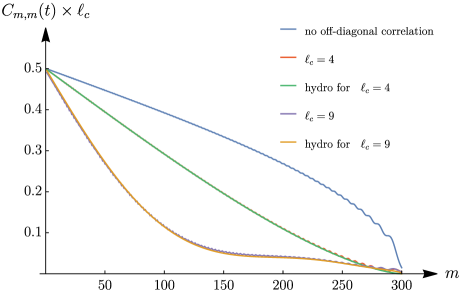
Figure 10: Density profile at $t=300$ in the right half-space for difference coherence length. For readability, all the curves have been rescaled by a factor $\ell_{c}$ to match at the origin.

Appendix B Full counting statistics in domain-wall states of lattice free fermions

In this appendix, we give an expression of the full counting statistics in the discrete domain wall in terms of a continuous kernel for a general correlated domain wall initial state, thus extending the recent results in [Moriya, Nagao and Sasamoto, JSTAT 2019(6):063105] on the one-dimensional XX spin chain.

The (homogeneous) FCS is defined for a subspace $\mathcal{S}$ as the generating function of the particle number operator in $\mathcal{S}$ at time $t$ i.e. $\hat{N}_{\mathcal{S}}(t)=\sum_{m\in\mathcal{S}}c_{m}^{\dagger}(t)c_{m}(t)$. It is by Wick’s theorem equal to a Fredholm determinant [98, 47, 48, 50]

$$\big{\langle}e^{\mathbf{i}\lambda\hat{N}_{\mathcal{S}}(t)}\big{\rangle}=\mathrm{Det}\left[1+(e^{\mathbf{i}\lambda}-1)\hat{C}(t)P_{\mathcal{S}}\right]_{\ell^{2}(\mathbb{Z})}$$ (65)

where $P_{\mathcal{S}}$ is the projector onto the subspace $\mathcal{S}$, and $\ell^{2}(\mathbb{Z})$ denotes the space of square-summable sequences on $\mathbb{Z}$. The FCS has been used in [48, 50] to make a very interesting connection between the statistics of free fermions and the statistics of eigenvalues in random matrix theory. In a larger scope, we note that connections with random matrix theory and stochastic systems also exist for other fermionic systems, namely non-interacting fermions in a range of classic potentials, see for instance Ref. [99, 100, 101].

In the following we will denote $z=e^{\mathbf{i}\lambda}-1$ and drop the time dependence in the kernels. We inject the expression of $\hat{C}$ given in Eq. (4) in terms of the initial correlations and the discrete kernel $\hat{J}$. We then use the general relation $\mathrm{det}(I+AB)=\mathrm{det}(I+BA)$ for arbitrary Hilbert-Schmidt operators $A$ and $B$ (this is the Sylvester’s identity, valid as long as the different products make sense [102]). This yields

$$\mathrm{Det}\left[1+z\hat{J}^{\dagger}\hat{C}_{0}\hat{J}P_{\mathcal{S}}\right]_{\ell^{2}(\mathbb{Z})}=\mathrm{Det}\left[1+z\hat{C}_{0}\hat{J}P_{\mathcal{S}}\hat{J}^{\dagger}\right]_{\ell^{2}(\mathbb{Z})}$$ (66)

Choosing the subspace $\mathcal{S}$ to be an interval $[a,b]$ with $0<a<b$, the operator $\hat{J}P_{\mathcal{S}}\hat{J}^{\dagger}$ is shown in Appendix B.1 to become

$$[\hat{J}P_{\mathcal{S}}\hat{J}^{\dagger}]_{n,m}=\mathbf{i}^{n-m}(B_{t}(m-b,n-b)-B_{t}(m-a+1,n-a+1))$$ (67)

where $B_{t}$ is the discrete integral operator acting on $\ell^{2}(\mathbb{Z})$ defined by the discrete Bessel kernel introduced previously (cf. Eq. (57)).

If we now assume that the interval is semi-infinite, i.e. $b=+\infty$, we have

$$[\hat{J}P_{\mathcal{S}}\hat{J}^{\dagger}]_{n,m}=-\mathbf{i}^{n-m}B_{t}(m-a+1,n-a+1)\mathrel{\mathop{\mathchar 58\relax}}=-\mathcal{B}_{n,m}$$ (68)

where we have introduced the notation $\mathcal{B}$ for this discrete kernel, which depends on $t$ and $a$. Hence we obtain the full counting statistics on an arbitrary interval for a general initial condition in terms of the discrete Bessel kernel as

$$\big{\langle}e^{\mathbf{i}\lambda\hat{N}_{\mathcal{S}}(t)}\big{\rangle}=\mathrm{Det}\left[1-z\,\hat{C}_{0}\,\mathcal{B}\right]_{\ell^{2}(\mathbb{Z})}$$ (69)

The form of this result Eq. (69) and in particular the operator $\mathcal{B}$, does not depend on the details of the initial condition, appearing only as the initial correlation matrix $\hat{C}_{0}$.

The integral operators we obtained so far acted on the lattice $\ell^{2}(\mathbb{Z})$. Moriya, Nagao and Sasamoto recently obtained in [50] that for the domain wall initial condition, the FCS $\big{\langle}e^{\mathbf{i}\lambda\hat{N}_{\mathcal{S}}(t)}\big{\rangle}$ can be seen as the determinant of the continuous Bessel kernel, acting on $\mathbb{L}^{2}(\mathbb{R^{+}})$, see Ref. [50, Eq. (3.8)]. This relation allowed them to make a connection with the Laguerre ensemble in random matrix theory and study the large deviations of the spin current. Here, we extend this result for any initial condition $\hat{C}_{0}$ supported on the left-side $\mathcal{L}$ and zero elsewhere, while we recall that the full counting statistics are studied on the subspace $\mathcal{S}=[a,+\infty)$ with $a>0$. In this view, we introduce the following semi-discrete kernels

$$\begin{split}&\tilde{J}_{1}(n,\tilde{t})=\left(\frac{\mathbf{i}t}{\sqrt{\tilde{t}}}\right)^{n-a}J_{n-a+1}(\sqrt{\tilde{t}})\;,\\ &\tilde{J}_{2}(\tilde{t},m)=\left(\frac{\mathbf{i}t}{\sqrt{\tilde{t}}}\right)^{a-m}J_{m-a}(\sqrt{\tilde{t}})\;.\end{split}$$ (70)

where $m$ and $n$ denote integers and $\tilde{t}$ denotes a real variable (the differing order of variables is chosen in order to write operator products in a natural way). Crucially, it is shown in Appendix B.2 that the following discrete-operator identity holds for every matrix element $(n,m)$

$$\hat{J}^{\dagger}P_{\mathcal{S}}\hat{J}=-\tilde{J}_{1}\tilde{J}_{2}$$ (71)

where the measure of integration in $\tilde{t}$ space is $\frac{1}{2}\int_{0}^{t^{2}}\frac{\mathrm{d}\tilde{t}}{\sqrt{\tilde{t}}}$, on the interval $[0,t^{2}]$. A straightforward application of Sylvester’s identity then gives

$$\mathrm{Det}\left[1-z\hat{C}_{0}\tilde{J}_{1}\tilde{J}_{2}\right]_{\ell^{2}(\mathbb{Z})}=\mathrm{Det}\left[1-z\tilde{J}_{2}\hat{C}_{0}\tilde{J}_{1}\right]_{\mathbb{L}^{2}(0,t^{2})}$$ (72)

such that finally

$$\big{\langle}e^{\mathbf{i}\lambda\hat{N}_{\mathcal{S}}(t)}\big{\rangle}=\mathrm{Det}\left[1+z\hat{J}^{\dagger}\hat{C}_{0}\hat{J}P_{\mathcal{S}}\right]_{\ell^{2}(\mathbb{Z})}=\mathrm{Det}\left[1-z\tilde{J}_{2}\hat{C}_{0}\tilde{J}_{1}\right]_{\mathbb{L}^{2}(0,t^{2})}\;.$$ (73)

If the initial state is the uncorrelated domain wall, $\hat{C}_{0}=\hat{C}_{0}^{\mathcal{D}}$ is the identity matrix when restricted to $\mathcal{L}$, and zero otherwise. In this case, $J^{\dagger}\hat{C}_{0}^{\mathcal{D}}JP_{\mathcal{S}}$ is easily shown to be the discrete Bessel kernel through computations similar to the ones that lead to Eq. (67). Furthermore, $-\tilde{J}_{2}\hat{C}_{0}^{\mathcal{D}}\tilde{J}_{1}$ is the continuous Bessel kernel as shown in Appendix B.3. As a consequence, Eq. (73) recovers the Moriya et al. identity connecting the discrete Bessel kernel to the continuous Bessel kernel. We note that our proof of this identity is substantially shorter than the one given in [50], which is centered on the computation of all moments of both kernels in order to establish the identity at the level of Fredholm determinants. In contrast, the introduction of semi-discrete kernels $\tilde{J}_{1,2}$ and the use of Sylvester’s identity allows us to avoid computations of arbitrary-order moments.

With a general initial condition, Eq. (73) is a generalization of the Moriya et al identity, Ref. [50, Eq. (3.8)], connecting a discrete kernel to a continuous kernel that depends on the initial condition. An interesting development of this study would be to find XX chain initial states leading, through Eq. (73), to other known random matrix theory kernels.

B.1 Derivation of Eq. (67)

In this subsection, we establish the Christoffel-Darboux identity for the discrete Bessel Kernel given in Eq. (67). We first write the following relation for the Bessel functions

$$\begin{split}J_{n-j}(t)J_{m-j}(t)&=\frac{t}{2(m-n)}\left(\frac{2}{t}[m-j-n+j]J_{n-j}(t)J_{m-j}(t)\right)\\ &=\frac{t}{2(m-n)}\left(\frac{2}{t}[m-j]J_{n-j}(t)J_{m-j}(t)-\frac{2}{t}[n-j]J_{n-j}(t)J_{m-j}(t)\right)\;.\end{split}$$ (74)

The recurrence relation of Bessel functions $(2\nu/z)J_{\nu}(z)=J_{\nu+1}(z)+J_{\nu-1}(z)$ [71] yields

$$\begin{split}J_{n-j}(t)J_{m-j}(t)&=\frac{t}{2(m-n)}\left(J_{n-j}(t)(J_{m-j+1}(t)+J_{m-j-1}(t))-(J_{n-j+1}(t)+J_{n-j-1}(t))J_{m-j}(t)\right)\\ &=\frac{t}{2(m-n)}\big{(}\left[J_{n-j}(t)J_{m-j+1}(t)-J_{n-j-1}(t)J_{m-j}(t)\right]\\ &\qquad\qquad\qquad+\left[J_{n-j}(t)J_{m-j-1}(t)-J_{n-j+1}(t)J_{m-j}(t)\right]\big{)}\;.\end{split}$$ (75)

This is the general term of a telescopic sum leading to the simplified equation

$$\begin{split}\sum\limits_{j=a}^{b}J_{n-j}(t)J_{m-j}(t)=\frac{t}{2(m-n)}&\big{(}\left[J_{n-a}(t)J_{m-a+1}(t)-J_{n-b-1}(t)J_{m-b}(t)\right]\\ &+\left[J_{n-b}(t)J_{m-b-1}(t)-J_{n-a+1}(t)J_{m-a}(t)\right]\big{)}\;.\end{split}$$ (76)

With the discrete Bessel kernel $B_{t}(m,n)$ defined in the main text, we finally recover Eq. (67) of the main text

$$\sum\limits_{j=a}^{b}J_{n-j}(t)J_{m-j}(t)=B_{t}(m-b,n-b)-B_{t}(m-a+1,n-a+1)\;.$$ (77)

B.2 Derivation of Eq. (71)

In this subsection, we establish the relation between discrete and semi-discrete kernels stated in Eq. (71). We will directly write the matrix element $(n,m)$ of $J^{\dagger}P_{\mathcal{S}}J$ and transform it using the contour integral expression of $J$ as $J_{k}(t)=\oint_{|z|=1}\frac{\mathrm{d}z}{2\mathbf{i}\pi z}e^{\frac{t}{2}(z-\frac{1}{z})}(-z)^{k}$, see Ref. [50, equations A.6-A.8]. We have:

$$\begin{split}&[\hat{J}^{\dagger}P_{\mathcal{S}}\hat{J}]_{n,m}=\mathbf{i}^{n-m}\sum_{k=a}^{b}J_{n-k}(t)J_{m-k}(t)\\ &=(-\mathbf{i})^{n-m}\oint_{|z_{1}|=1}\oint_{|z_{2}|=1}\frac{\mathrm{d}z_{1}}{2\mathbf{i}\pi}\frac{\mathrm{d}z_{2}}{2\mathbf{i}\pi}e^{\frac{t}{2}(z_{2}-\frac{1}{z_{1}})}\sum_{k=a}^{b}\frac{e^{\frac{t}{2}(z_{1}-\frac{1}{z_{2}})}}{z_{1}^{k-n+1}z_{2}^{k-m+1}}\\ &=\frac{\mathbf{i}^{m-n}}{2}\oint_{|z_{1}|=1}\oint_{|z_{2}|=1}\frac{\mathrm{d}z_{1}}{2\mathbf{i}\pi}\frac{\mathrm{d}z_{2}}{2\mathbf{i}\pi}e^{\frac{t}{2}(z_{2}-\frac{1}{z_{1}})}\frac{1}{z_{1}^{-n+1}z_{2}^{-m+1}}\left(\int_{0}^{t}\mathrm{d}t_{1}e^{\frac{t_{1}}{2}(z_{1}-\frac{1}{z_{2}})}-\frac{2}{z_{1}-\frac{1}{z_{2}}}\right)\sum_{k=a}^{b}\left(\frac{1}{z_{1}^{k-1}z_{2}^{k}}-\frac{1}{z_{1}^{k}z_{2}^{k+1}}\right)\end{split}$$ (78)

where we can drop a term because it leads to an integrand without poles with respect to the complex variables $z_{1}$ and $z_{2}$, see [50], such that

$$\begin{split}[\hat{J}^{\dagger}P_{\mathcal{S}}\hat{J}]_{n,m}&=\frac{\mathbf{i}^{m-n}}{2}\oint_{|z_{1}|=1}\oint_{|z_{2}|=1}\frac{\mathrm{d}z_{1}}{2\mathbf{i}\pi}\frac{\mathrm{d}z_{2}}{2\mathbf{i}\pi}e^{\frac{t}{2}(z_{2}-\frac{1}{z_{1}})}\frac{1}{z_{1}^{-n+1}z_{2}^{-m+1}}\int_{0}^{t}\mathrm{d}t_{1}e^{\frac{t_{1}}{2}(z_{1}-\frac{1}{z_{2}})}\left[\frac{1}{z_{1}^{a-1}z_{2}^{a}}-\frac{1}{z_{1}^{b}z_{2}^{b+1}}\right]\\ &=\frac{\mathbf{i}^{m-n}}{2}\int_{0}^{t}\mathrm{d}t_{1}\oint_{|z_{1}|=1}\oint_{|z_{2}|=1}\frac{\mathrm{d}z_{1}}{2\mathbf{i}\pi}\frac{\mathrm{d}z_{2}}{2\mathbf{i}\pi}e^{\frac{t}{2}(z_{2}-\frac{1}{z_{1}})}e^{\frac{t_{1}}{2}(z_{1}-\frac{1}{z_{2}})}\left[\frac{1}{z_{1}^{a-n}z_{2}^{a-m+1}}-\frac{1}{z_{1}^{b-n+1}z_{2}^{b-m+2}}\right]\\ \end{split}$$ (79)

Upon rescaling $z_{2}=\tilde{z}_{2}\sqrt{\frac{t_{1}}{t}}$ and $z_{1}=\tilde{z}_{1}\sqrt{\frac{t}{t_{1}}}$, one obtains

$$\begin{split}[\hat{J}^{\dagger}P_{\mathcal{S}}\hat{J}]_{n,m}=&\frac{\mathbf{i}^{m-n}}{2}\int_{0}^{t}\mathrm{d}t_{1}\oint_{|\tilde{z}_{1}|=\sqrt{\frac{t_{1}}{t}}}\oint_{|\tilde{z}_{2}|=\sqrt{\frac{t}{t_{1}}}}\frac{\mathrm{d}\tilde{z}_{1}}{2\mathbf{i}\pi}\frac{\mathrm{d}\tilde{z}_{2}}{2\mathbf{i}\pi}\left(\sqrt{\frac{t}{t_{1}}}\right)^{n-m+1}e^{\frac{\sqrt{tt_{1}}}{2}(\tilde{z}_{1}-\frac{1}{\tilde{z}_{1}}+\tilde{z}_{2}-\frac{1}{\tilde{z}_{2}})}\\ &\left[\frac{1}{\tilde{z}_{1}^{a-n}\tilde{z}_{2}^{a-m+1}}-\frac{1}{\tilde{z}_{1}^{b-n+1}\tilde{z}_{2}^{b-m+2}}\right]\\ =&-\frac{\mathbf{i}^{n-m}}{2}\int_{0}^{t}\mathrm{d}t_{1}\left(\sqrt{\frac{t}{t_{1}}}\right)^{n-m+1}\left(J_{n-a+1}(\sqrt{tt_{1}})J_{m-a}(\sqrt{tt_{1}})-J_{n-b}(\sqrt{tt_{1}})J_{m-b-1}(\sqrt{tt_{1}})\right)\\ \end{split}$$ (80)

where we assumed that $n,m\notin[a,b]$ such that $[J^{\dagger}P_{\mathcal{A}}J]_{n,m}(t=0)=0$. Let us now push $b\to\infty$ such that the corresponding boundary terms disappear. We also rescale $t_{1}=\tilde{t}/t$ such that

$$[\hat{J}^{\dagger}P_{\mathcal{S}}\hat{J}]_{n,m}=-\frac{(\mathbf{i}t)^{n-m}}{2}\int_{0}^{t^{2}}\mathrm{d}\tilde{t}\;\tilde{t}^{\frac{a-n-1}{2}}J_{n-a+1}\left(\sqrt{\tilde{t}}\right)J_{m-a}\left(\sqrt{\tilde{t}}\right)\tilde{t}^{-\frac{a-m}{2}}$$ (81)

We see that we can rewrite $J^{\dagger}P_{\mathcal{S}}J=-\tilde{J}_{1}\tilde{J}_{2}$ where $\tilde{J}_{1,2}$ are semi-discrete integral operators with kernels

$$\begin{split}&\tilde{J}_{1}(n,\tilde{t})=\left(\frac{\mathbf{i}t}{\sqrt{\tilde{t}}}\right)^{n-a}J_{n-a+1}\left(\sqrt{\tilde{t}}\right)\\ &\tilde{J}_{2}(\tilde{t},m)=\left(\frac{\mathbf{i}t}{\sqrt{\tilde{t}}}\right)^{a-m}J_{m-a}\left(\sqrt{\tilde{t}}\right)\\ \end{split}$$ (82)

where the measure of integration is $\frac{1}{2}\int_{0}^{t^{2}}\frac{\mathrm{d}\tilde{t}}{\sqrt{\tilde{t}}}$, on the interval $[0,t^{2}]$. We have thus established Eq. (71).

B.3 Recovering the Moriya et al identity for the uncorrelated domain-wall

In this subsection we show that, in the case of the uncorrelated domain-wall initial condition where $\hat{C}_{0}=P_{\mathbb{Z^{-}}}$, the kernel $-\tilde{J}_{2}\hat{C}_{0}\tilde{J}_{1}$ in the Fredholm determinant of Eq. (73) coincides with the continuous Bessel kernel. The goal of the derivation is to show that our introduction of semi-discrete kernels is a way to recover the results of [50] in the case of the uncorrelated domain-wall initial condition. More precisely, we wish to establish the following identity

$$[-\tilde{J}_{2}\hat{C}_{0}\tilde{J}_{1}](t_{1},t_{2})=\left(\sqrt{\frac{t_{2}}{t_{1}}}\right)^{a}\sqrt{t_{1}}\ \ \frac{\sqrt{t_{1}}J_{a-1}^{\prime}(\sqrt{t_{1}})J_{a-1}(\sqrt{t_{2}})-\sqrt{t_{2}}J_{a-1}(\sqrt{t_{1}})J_{a-1}^{\prime}(\sqrt{t_{2}})}{t_{1}-t_{2}}$$ (83)

where the domain-wall initial condition $\hat{C}_{0}=P_{\mathbb{Z^{-}}}$ gives the left-hand side as

$$[-\tilde{J}_{2}\hat{C}_{0}\tilde{J}_{1}](t_{1},t_{2})=-\sum_{k\in\mathbb{Z}^{-}}\left(\sqrt{\frac{t_{2}}{t_{1}}}\right)^{a-k}J_{k-a}(\sqrt{t_{1}})J_{k-a+1}(\sqrt{t_{2}})\;.$$ (84)

Indexing the sum by the natural integers and inserting the contour integral representation of the Bessel function introduced in the previous section, we have

$$\begin{split}[-\tilde{J}_{2}\hat{C}_{0}\tilde{J}_{1}](t_{1},t_{2})&=-\sum_{k\in\mathbb{N}}\left(\sqrt{\frac{t_{2}}{t_{1}}}\right)^{a+k}J_{-k-a}(\sqrt{t_{1}})J_{-k-a+1}(\sqrt{t_{2}})\\ &=\oint_{|z_{1}|=1}\oint_{|z_{2}|=1}\frac{\mathrm{d}z_{1}}{2\mathbf{i}\pi}\frac{\mathrm{d}z_{2}}{2\mathbf{i}\pi}\sum_{k\in\mathbb{N}}\left(\sqrt{\frac{t_{2}}{t_{1}}}\right)^{a+k}\frac{1}{z_{1}^{a+k+1}z_{2}^{a+k}}e^{\frac{\sqrt{t_{1}}}{2}(z_{1}-\frac{1}{z_{1}})+\frac{\sqrt{t_{2}}}{2}(z_{2}-\frac{1}{z_{2}})}\end{split}$$ (85)

The change of variables $\tilde{z}_{1}=\frac{z_{1}}{\sqrt{t_{2}}},\tilde{z}_{2}=\sqrt{t_{1}}z_{2}$ yields

$$\begin{split}&[-\tilde{J}_{2}\hat{C}_{0}\tilde{J}_{1}](t_{1},t_{2})=\\ &\frac{1}{\sqrt{t_{1}}}\oint_{|\tilde{z}_{1}|=\frac{1}{\sqrt{t_{2}}}}\oint_{|\tilde{z}_{2}|=\sqrt{t_{1}}}\frac{\mathrm{d}\tilde{z}_{1}}{2\mathbf{i}\pi}\frac{\mathrm{d}\tilde{z}_{2}}{2\mathbf{i}\pi}\sum_{k\in\mathbb{N}}\frac{1}{\tilde{z}_{1}^{a+k+1}\tilde{z}_{2}^{a+k}}e^{\frac{\sqrt{t_{1}t_{2}}}{2}(\tilde{z}_{1}-\frac{1}{\tilde{z}_{2}})-\sqrt{\frac{t_{1}}{t_{2}}}\frac{1}{2\tilde{z}_{1}}+\sqrt{\frac{t_{2}}{t_{1}}}\frac{\tilde{z}_{2}}{2}}\\ &=\frac{1}{\sqrt{t_{1}}}\oint_{|\tilde{z}_{1}|=\frac{1}{\sqrt{t_{2}}}}\oint_{|\tilde{z}_{2}|=\sqrt{t_{1}}}\frac{\mathrm{d}\tilde{z}_{1}}{2\mathbf{i}\pi}\frac{\mathrm{d}\tilde{z}_{2}}{2\mathbf{i}\pi}\frac{e^{-\sqrt{\frac{t_{1}}{t_{2}}}\frac{1}{2\tilde{z}_{1}}+\sqrt{\frac{t_{2}}{t_{1}}}\frac{\tilde{z}_{2}}{2}}}{\tilde{z}_{1}(\tilde{z}_{1}\tilde{z}_{2})^{a}}\sum_{k\in\mathbb{N}}\frac{1}{(\tilde{z}_{1}\tilde{z}_{2})^{k}}\left(\frac{1}{2}\int_{0}^{\sqrt{t_{1}t_{2}}}\mathrm{d}\tilde{t}\ e^{\frac{\tilde{t}}{2}(\tilde{z}_{1}-\frac{1}{\tilde{z}_{2}})}\left(\tilde{z}_{1}-\frac{1}{\tilde{z}_{2}}\right)+1\right)\\ &=\frac{1}{\sqrt{t_{1}}}\oint_{|\tilde{z}_{1}|=\frac{1}{\sqrt{t_{2}}}}\oint_{|\tilde{z}_{2}|=\sqrt{t_{1}}}\frac{\mathrm{d}\tilde{z}_{1}}{2\mathbf{i}\pi}\frac{\mathrm{d}\tilde{z}_{2}}{2\mathbf{i}\pi}\frac{e^{-\sqrt{\frac{t_{1}}{t_{2}}}\frac{1}{2\tilde{z}_{1}}+\sqrt{\frac{t_{2}}{t_{1}}}\frac{\tilde{z}_{2}}{2}}}{\tilde{z}_{1}(\tilde{z}_{1}\tilde{z}_{2})^{a}}\sum_{k\in\mathbb{N}}\frac{1}{2}\int_{0}^{\sqrt{t_{1}t_{2}}}\mathrm{d}\tilde{t}\ e^{\frac{\tilde{t}}{2}(\tilde{z}_{1}-\frac{1}{\tilde{z}_{2}})}\left(\frac{1}{\tilde{z}_{1}^{k-1}\tilde{z}_{2}^{k}}-\frac{1}{\tilde{z}_{1}^{k}\tilde{z}_{2}^{k+1}}\right)\end{split}$$ (86)

where we have dropped the +1 term in the last equation, as it leads to a null contribution in the contour integrals. The telescopic sum simplifies such that

$$\begin{split}[-\tilde{J}_{2}\hat{C}_{0}\tilde{J}_{1}](t_{1},t_{2})&=\frac{1}{\sqrt{t_{1}}}\oint_{|\tilde{z}_{1}|=\frac{1}{\sqrt{t_{2}}}}\oint_{|\tilde{z}_{2}|=\sqrt{t_{1}}}\frac{\mathrm{d}\tilde{z}_{1}}{2\mathbf{i}\pi}\frac{\mathrm{d}\tilde{z}_{2}}{2\mathbf{i}\pi}\frac{e^{-\sqrt{\frac{t_{1}}{t_{2}}}\frac{1}{2\tilde{z}_{1}}+\sqrt{\frac{t_{2}}{t_{1}}}\frac{\tilde{z}_{2}}{2}}}{\tilde{z}_{1}(\tilde{z}_{1}\tilde{z}_{2})^{a}}\frac{1}{2}\int_{0}^{\sqrt{t_{1}t_{2}}}\mathrm{d}\tilde{t}\ e^{\frac{\tilde{t}}{2}(\tilde{z}_{1}-\frac{1}{\tilde{z}_{2}})}\tilde{z}_{1}\\ &=\frac{1}{2\sqrt{t_{1}}}\int_{0}^{\sqrt{t_{1}t_{2}}}\mathrm{d}\tilde{t}\oint_{|\tilde{z}_{1}|=\frac{1}{\sqrt{t_{2}}}}\oint_{|\tilde{z}_{2}|=\sqrt{t_{1}}}\frac{\mathrm{d}\tilde{z}_{1}}{2\mathbf{i}\pi}\frac{\mathrm{d}\tilde{z}_{2}}{2\mathbf{i}\pi}\frac{1}{(\tilde{z}_{1}\tilde{z}_{2})^{a}}e^{\frac{\tilde{t}}{2}(\tilde{z}_{1}-\frac{1}{\tilde{z}_{2}})}e^{-\sqrt{\frac{t_{1}}{t_{2}}}\frac{1}{2\tilde{z}_{1}}+\sqrt{\frac{t_{2}}{t_{1}}}\frac{\tilde{z}_{2}}{2}}\end{split}$$ (87)

Scaling to $\tau=\frac{\tilde{t}}{\sqrt{t_{1}t_{2}}}$, we have

$$[-\tilde{J}_{2}\hat{C}_{0}\tilde{J}_{1}](t_{1},t_{2})=\frac{\sqrt{t_{2}}}{2}\int_{0}^{1}\mathrm{d}\tau\oint_{|\tilde{z}_{1}|=\frac{1}{\sqrt{t_{2}}}}\oint_{|\tilde{z}_{2}|=\sqrt{t_{1}}}\frac{\mathrm{d}\tilde{z}_{1}}{2\mathbf{i}\pi}\frac{\mathrm{d}\tilde{z}_{2}}{2\mathbf{i}\pi}\frac{1}{(\tilde{z}_{1}\tilde{z}_{2})^{a}}e^{\frac{\tau\sqrt{t_{1}t_{2}}}{2}(\tilde{z}_{1}-\frac{1}{\tilde{z}_{2}})}e^{-\sqrt{\frac{t_{1}}{t_{2}}}\frac{1}{2\tilde{z}_{1}}+\sqrt{\frac{t_{2}}{t_{1}}}\frac{\tilde{z}_{2}}{2}}$$ (88)

Changing variables again to $\accentset{\approx}{z}_{1}=\sqrt{t_{2}\tau}\tilde{z}_{1}$ and $\accentset{\approx}{z}_{2}=\frac{1}{\sqrt{t_{1}\tau}}\tilde{z}_{2}$, we obtain

$$[-\tilde{J}_{2}\hat{C}_{0}\tilde{J}_{1}](t_{1},t_{2})=\frac{\sqrt{t_{1}}}{2}\left(\sqrt{\frac{t_{2}}{t_{1}}}\right)^{a}\int_{0}^{1}\mathrm{d}\tau\oint_{|\accentset{\approx}{z}_{1}|=\sqrt{\tau}}\oint_{|\accentset{\approx}{z}_{2}|=\frac{1}{\sqrt{\tau}}}\frac{\mathrm{d}\accentset{\approx}{z}_{1}}{2\mathbf{i}\pi}\frac{\mathrm{d}\accentset{\approx}{z}_{2}}{2\mathbf{i}\pi}\frac{1}{(\accentset{\approx}{z}_{1}\accentset{\approx}{z}_{2})^{a}}e^{\frac{\sqrt{\tau t_{1}}}{2}(\accentset{\approx}{z}_{1}-\frac{1}{\accentset{\approx}{z}_{1}})+\frac{\sqrt{\tau t_{2}}}{2}(\accentset{\approx}{z}_{2}-\frac{1}{\accentset{\approx}{z}_{2}})}$$ (89)

such that finally, evaluating the contour integrals to Bessel functions and introducing $\tilde{\tau}=\sqrt{\tau}$:

$$\begin{split}[-\tilde{J}_{2}\hat{C}_{0}\tilde{J}_{1}](t_{1},t_{2})=\frac{\sqrt{t_{1}}}{2}\sqrt{\frac{t_{2}}{t_{1}}}^{a}\int_{0}^{1}J_{a-1}(\sqrt{\tau t_{1}})J_{a-1}(\sqrt{\tau t_{2}})\mathrm{d}\tau=\sqrt{t_{1}}\left(\sqrt{\frac{t_{2}}{t_{1}}}\right)^{a}\int_{0}^{1}\tilde{\tau}J_{a-1}(\tilde{\tau}\sqrt{t_{1}})J_{a-1}(\tilde{\tau}\sqrt{t_{2}})\mathrm{d}\tilde{\tau}\end{split}$$ (90)

This is readily computed from known integrals [71], and simplified to

$$\begin{split}&[-\tilde{J}_{2}\hat{C}_{0}\tilde{J}_{1}](t_{1},t_{2})=\sqrt{t_{1}}\left(\sqrt{\frac{t_{2}}{t_{1}}}\right)^{a}\frac{\sqrt{t_{1}}J_{a}(\sqrt{t_{1}})J_{a-1}(\sqrt{t_{2}})-\sqrt{t_{2}}J_{a-1}(\sqrt{t_{1}})J_{a}(\sqrt{t_{2}})}{t_{1}-t_{2}}\\ &=\sqrt{t_{1}}\left(\sqrt{\frac{t_{2}}{t_{1}}}\right)^{a}\frac{\sqrt{t_{1}}\left(J_{a-1}^{\prime}(\sqrt{t_{1}})+\frac{a-1}{\sqrt{t_{1}}}J_{a-1}(\sqrt{t_{1}})\right)J_{a-1}(\sqrt{t_{2}})-\sqrt{t_{2}}J_{a-1}(\sqrt{t_{1}})\left(J_{a-1}^{\prime}(\sqrt{t_{2}})+\frac{a-1}{\sqrt{t_{2}}}J_{a-1}(\sqrt{t_{2}})\right)}{t_{1}-t_{2}}\\ &=\sqrt{t_{1}}\left(\sqrt{\frac{t_{2}}{t_{1}}}\right)^{a}\frac{\sqrt{t_{1}}J_{a-1}^{\prime}(\sqrt{t_{1}})J_{a-1}(\sqrt{t_{2}})-\sqrt{t_{2}}J_{a-1}(\sqrt{t_{1}})J_{a-1}^{\prime}(\sqrt{t_{2}})}{t_{1}-t_{2}}\end{split}$$ (91)

This concludes the derivation of Eq. (83).

Appendix C Transport measure in the continuous setting

We prove here the formula giving the slope as a function of the Wigner function Eq. (23). Let $n(x,k,t)$ be a Wigner function so that its initial condition and evolution read

$$n(x,k,t=0)=n^{{\rm eq}}(x,k),\qquad n(x,k,t)=n^{{\rm eq}}(x-kt,k)\,.$$ (92)

The density profile at any given position $x$ and time $t$ is obtained as

$$\varrho(x,t)=\int_{x/t}^{\infty}\frac{\mathrm{d}k}{2\pi}n(x,k)$$ (93)

and the total number of particles in the right half-space at a given time

$$N_{{\cal R}}(t) =\int_{0}^{\infty}\varrho(x,t)\mathrm{d}x$$ (94)

$$=\int_{0}^{\infty}\int_{x/t}^{\infty}n^{{\rm eq}}(x,k)\frac{\mathrm{d}k}{2\pi}\mathrm{d}x$$ (95)

$$=\int_{0}^{\infty}\int_{1}^{\infty}n^{{\rm eq}}(x,\frac{x}{t}k^{\prime})\frac{x}{t}\frac{\mathrm{d}k^{\prime}}{2\pi}\mathrm{d}x$$ (96)

$$=\int_{0}^{\infty}\int_{1}^{\infty}n^{{\rm eq}}(\frac{x}{t}k^{\prime})\frac{x}{t}\frac{\mathrm{d}k^{\prime}}{2\pi}\mathrm{d}x$$ (97)

$$=t\int_{0}^{\infty}\int_{1}^{\infty}n^{{\rm eq}}(x^{\prime}k^{\prime})x^{\prime}\frac{\mathrm{d}k^{\prime}}{2\pi}\mathrm{d}x^{\prime}$$ (98)

$$=t\int_{0}^{\infty}\int_{1}^{\infty}n^{{\rm eq}}(X)\frac{X}{k^{\prime 2}}\frac{\mathrm{d}k^{\prime}}{2\pi}\mathrm{d}X$$ (99)

$$=t\int_{0}^{\infty}n^{{\rm eq}}(X)X\frac{1}{2\pi}\mathrm{d}X$$ (100)

where we made the serie of substitutions $k^{\prime}=k\frac{t}{x}$ and $x^{\prime}=x/t$, $X=x^{\prime}k^{\prime}$ We also suppose that the $x$ dependence of $n^{{\rm eq}}(x,k)$ is always of the form $\Theta(-x)n(k)$. We thus see that the dependence in time is linear no matter what and the slope is given by :

$$\mu_{T}(n^{{\rm eq}})\mathrel{\mathop{\mathchar 58\relax}}=\int_{0}^{\infty}\frac{dk}{2\pi}kn^{{\rm eq}}(k)$$ (101)

which has the simple interpretation of the sum over all propagating modes indexed by $k$ weighted by their velocity $\frac{\mathrm{d}\epsilon(k)}{\mathrm{d}k}=k$.

References

- [1] Manuel Endres, Hannes Bernien, Alexander Keesling, Harry Levine, Eric R Anschuetz, Alexandre Krajenbrink, Crystal Senko, Vladan Vuletic, Markus Greiner, and Mikhail D Lukin. Atom-by-atom assembly of defect-free one-dimensional cold atom arrays. Science, 354(6315):1024–1027, 2016.
- [2] Sepehr Ebadi, Tout T Wang, Harry Levine, Alexander Keesling, Giulia Semeghini, Ahmed Omran, Dolev Bluvstein, Rhine Samajdar, Hannes Pichler, Wen Wei Ho, et al. Quantum phases of matter on a 256-atom programmable quantum simulator. arXiv preprint arXiv:2012.12281, 2020.
- [3] Pascal Scholl, Michael Schuler, Hannah J Williams, Alexander A Eberharter, Daniel Barredo, Kai-Niklas Schymik, Vincent Lienhard, Louis-Paul Henry, Thomas C Lang, Thierry Lahaye, et al. Programmable quantum simulation of 2d antiferromagnets with hundreds of rydberg atoms. arXiv preprint arXiv:2012.12268, 2020.
- [4] B. Bakkali-Hassani, C. Maury, Y.Q. Zou, E. Le Cerf, R. Saint-Jalm, P.C.M. Castilho, S. Nascimbene, J. Dalibard, and J. Beugnon. Realization of a Townes Soliton in a Two-Component Planar Bose Gas. Arxiv preprint arXiv:2103.01605, 2021.
- [5] Hannes Bernien, Sylvain Schwartz, Alexander Keesling, Harry Levine, Ahmed Omran, Hannes Pichler, Soonwon Choi, Alexander S. Zibrov, Manuel Endres, Markus Greiner, Vladan Vuletić, and Mikhail D. Lukin. Probing many-body dynamics on a 51-atom quantum simulator. Nature, 551(7682):579–584, Nov 2017.
- [6] D. Bluvstein, A. Omran, H. Levine, A. Keesling, G. Semeghini, S. Ebadi, T. T. Wang, A. A. Michailidis, N. Maskara, W. W. Ho, S. Choi, M. Serbyn, M. Greiner, V. Vuletić, and M. D. Lukin. Controlling quantum many-body dynamics in driven rydberg atom arrays. Science, 371(6536):1355–1359, 2021.
- [7] Loïc Henriet, Lucas Beguin, Adrien Signoles, Thierry Lahaye, Antoine Browaeys, Georges-Olivier Reymond, and Christophe Jurczak. Quantum computing with neutral atoms. Quantum, 4:327, September 2020.
- [8] Bertrand Evrard, An Qu, Jean Dalibard, and Fabrice Gerbier. Production and characterization of a fragmented spinor bose-einstein condensate, 2020.
- [9] P. Alexander Bouvrie, Eloisa Cuestas, Itzhak Roditi, and Ana P. Majtey. Entanglement between two spatially separated ultracold interacting fermi gases. Phys. Rev. A, 99:063601, Jun 2019.
- [10] T. Antal, Z. Rácz, A. Rákos, and G. M. Schütz. Transport in the chain at zero temperature: Emergence of flat magnetization profiles. Phys. Rev. E, 59:4912–4918, May 1999.
- [11] Yoshiko Ogata. Nonequilibrium properties in the transverse chain. Phys. Rev. E, 66:016135, Jul 2002.
- [12] Andrea De Luca, Jacopo Viti, Denis Bernard, and Benjamin Doyon. Nonequilibrium thermal transport in the quantum ising chain. Phys. Rev. B, 88:134301, Oct 2013.
- [13] Mario Collura and Gabriele Martelloni. Non-equilibrium transport in d-dimensional non-interacting fermi gases. Journal of Statistical Mechanics: Theory and Experiment, 2014(8):P08006, aug 2014.
- [14] Mario Collura and Dragi Karevski. Quantum quench from a thermal tensor state: Boundary effects and generalized gibbs ensemble. Phys. Rev. B, 89:214308, Jun 2014.
- [15] Jacopo Viti, Jean-Marie Stéphan, Jérôme Dubail, and Masudul Haque. Inhomogeneous quenches in a free fermionic chain: Exact results. EPL (Europhysics Letters), 115(4):40011, aug 2016.
- [16] Márton Kormos. Inhomogeneous quenches in the transverse field Ising chain: scaling and front dynamics. SciPost Phys., 3:020, 2017.
- [17] Oleksandr Gamayun, Oleg Lychkovskiy, and Jean-Sébastien Caux. Fredholm determinants, full counting statistics and Loschmidt echo for domain wall profiles in one-dimensional free fermionic chains. SciPost Phys., 8:36, 2020.
- [18] Gabriele Perfetto and Andrea Gambassi. Ballistic front dynamics after joining two semi-infinite quantum ising chains. Phys. Rev. E, 96:012138, Jul 2017.
- [19] Ulrich Heinz and Raimond Snellings. Collective flow and viscosity in relativistic heavy-ion collisions. Annual Review of Nuclear and Particle Science, 63(1):123–151, October 2013.
- [20] Markus Müller, Jörg Schmalian, and Lars Fritz. Graphene: A nearly perfect fluid. Phys. Rev. Lett., 103:025301, Jul 2009.
- [21] Olalla A. Castro-Alvaredo, Benjamin Doyon, and Takato Yoshimura. Emergent hydrodynamics in integrable quantum systems out of equilibrium. Phys. Rev. X, 6:041065, Dec 2016.
- [22] Bruno Bertini, Mario Collura, Jacopo De Nardis, and Maurizio Fagotti. Transport in out-of-equilibrium chains: Exact profiles of charges and currents. Phys. Rev. Lett., 117:207201, Nov 2016.
- [23] Benjamin Doyon, Takato Yoshimura, and Jean-Sébastien Caux. Soliton gases and generalized hydrodynamics. Phys. Rev. Lett., 120:045301, Jan 2018.
- [24] Benjamin Doyon and Herbert Spohn. Drude Weight for the Lieb-Liniger Bose Gas. SciPost Phys., 3:039, 2017.
- [25] Jacopo De Nardis, Denis Bernard, and Benjamin Doyon. Hydrodynamic diffusion in integrable systems. Phys. Rev. Lett., 121:160603, Oct 2018.
- [26] M. Schemmer, I. Bouchoule, B. Doyon, and J. Dubail. Generalized hydrodynamics on an atom chip. Phys. Rev. Lett., 122:090601, Mar 2019.
- [27] Neel Malvania, Yicheng Zhang, Yuan Le, Jerome Dubail, Marcos Rigol, and David S. Weiss. Generalized hydrodynamics in strongly interacting 1d bose gases, 2020.
- [28] Herbert Spohn. Large Scale Dynamics of Interacting Particles. Springer Berlin Heidelberg, 1991.
- [29] Maurizio Fagotti. Higher-order generalized hydrodynamics in one dimension: The noninteracting test. Phys. Rev. B, 96:220302, Dec 2017.
- [30] Maurizio Fagotti. Locally quasi-stationary states in noninteracting spin chains. SciPost Phys., 8:48, 2020.
- [31] Paola Ruggiero, Yannis Brun, and Jérôme Dubail. Conformal field theory on top of a breathing one-dimensional gas of hard core bosons. SciPost Phys., 6:51, 2019.
- [32] Paola Ruggiero, Pasquale Calabrese, Benjamin Doyon, and Jérôme Dubail. Quantum generalized hydrodynamics. Phys. Rev. Lett., 124:140603, Apr 2020.
- [33] Benjamin Doyon, Jérôme Dubail, Robert Konik, and Takato Yoshimura. Large-scale description of interacting one-dimensional bose gases: Generalized hydrodynamics supersedes conventional hydrodynamics. Physical review letters, 119(19):195301, 2017.
- [34] J.-P. Brantut, C. Grenier, J. Meineke, D. Stadler, S. Krinner, C. Kollath, T. Esslinger, and A. Georges. A thermoelectric heat engine with ultracold atoms. Science, 342(6159):713–715, October 2013.
- [35] E. Wigner. On the quantum correction for thermodynamic equilibrium. Phys. Rev., 40:749–759, Jun 1932.
- [36] MOSM Hillery, Robert F O’Connell, Marlan O Scully, and Eugene P Wigner. Distribution functions in physics: fundamentals. Physics reports, 106(3):121–167, 1984.
- [37] Kevin E Cahill and Roy J Glauber. Density operators and quasiprobability distributions. Physical Review, 177(5):1882, 1969.
- [38] E Bettelheim, AG Abanov, and P Wiegmann. Orthogonality catastrophe and shock waves in a nonequilibrium fermi gas. Physical review letters, 97(24):246402, 2006.
- [39] Eldad Bettelheim, Alexander G Abanov, and Paul B Wiegmann. Quantum hydrodynamics and nonlinear differential equations for degenerate fermi gas. Journal of Physics A: Mathematical and Theoretical, 41(39):392003, 2008.
- [40] Eldad Bettelheim and Paul B Wiegmann. Universal fermi distribution of semiclassical nonequilibrium fermi states. Physical Review B, 84(8):085102, 2011.
- [41] Eldad Bettelheim and Leonid Glazman. Quantum ripples over a semiclassical shock. Physical review letters, 109(26):260602, 2012.
- [42] IV Protopopov, DB Gutman, P Schmitteckert, and AD Mirlin. Dynamics of waves in one-dimensional electron systems: Density oscillations driven by population inversion. Physical Review B, 87(4):045112, 2013.
- [43] David S Dean, Pierre Le Doussal, Satya N Majumdar, and Gregory Schehr. Wigner function of noninteracting trapped fermions. Physical Review A, 97(6):063614, 2018.
- [44] Josef Weinbub and DK Ferry. Recent advances in wigner function approaches. Applied Physics Reviews, 5(4):041104, 2018.
- [45] JE Moyal. Stochastic processes and statistical physics. Journal of the Royal Statistical Society. Series B (Methodological), 11(2):150–210, 1949.
- [46] Leonid S. Levitov, Hyunwoo Lee, and Gordey B. Lesovik. Electron counting statistics and coherent states of electric current. Journal of Mathematical Physics, 37(10):4845–4866, October 1996.
- [47] K. Schönhammer. Full counting statistics for noninteracting fermions: Exact results and the levitov-lesovik formula. Phys. Rev. B, 75:205329, May 2007.
- [48] Viktor Eisler and Zoltán Rácz. Full counting statistics in a propagating quantum front and random matrix spectra. Phys. Rev. Lett., 110:060602, Feb 2013.
- [49] Takato Yoshimura. Full counting statistics in the free dirac theory. Journal of Physics A: Mathematical and Theoretical, 51(47):475002, oct 2018.
- [50] Hiroki Moriya, Rikuo Nagao, and Tomohiro Sasamoto. Exact large deviation function of spin current for the one dimensional XX spin chain with domain wall initial condition. Journal of Statistical Mechanics: Theory and Experiment, 2019(6):063105, jun 2019.
- [51] Oleksandr Gamayun, Oleg Lychkovskiy, and Jean-Sébastien Caux. Fredholm determinants, full counting statistics and Loschmidt echo for domain wall profiles in one-dimensional free fermionic chains. SciPost Phys., 8:36, 2020.
- [52] Gabriele Perfetto and Andrea Gambassi. Dynamics of large deviations in the hydrodynamic limit: Noninteracting systems. Phys. Rev. E, 102:042128, Oct 2020.
- [53] Viktor Eisler. Crossover between ballistic and diffusive transport: the quantum exclusion process. Journal of Statistical Mechanics: Theory and Experiment, 2011(06):P06007, Jun 2011.
- [54] M. Bauer, D. Bernard, and T. Jin. Equilibrium Fluctuations in Maximally Noisy Extended Quantum Systems. SciPost Phys., 6:45, 2019.
- [55] Denis Bernard and Tony Jin. Open quantum symmetric simple exclusion process. Phys. Rev. Lett., 123:080601, Aug 2019.
- [56] Tony Jin, Alexandre Krajenbrink, and Denis Bernard. From stochastic spin chains to quantum kardar-parisi-zhang dynamics. Phys. Rev. Lett., 125:040603, Jul 2020.
- [57] Maurizio Fagotti and Pasquale Calabrese. Evolution of entanglement entropy following a quantum quench: Analytic results for the chain in a transverse magnetic field. Phys. Rev. A, 78:010306, Jul 2008.
- [58] Bruno Bertini, Maurizio Fagotti, Lorenzo Piroli, and Pasquale Calabrese. Entanglement evolution and generalised hydrodynamics: noninteracting systems. J. Phys. A: Math. Theor., 51(39):39LT01, aug 2018.
- [59] Vincenzo Alba and Pasquale Calabrese. Entanglement and thermodynamics after a quantum quench in integrable systems. PNAS, 114(30):7947–7951, 2017.
- [60] Vincenzo Alba and Pasquale Calabrese. Entanglement dynamics after quantum quenches in generic integrable systems. SciPost Phys., 4:17, 2018.
- [61] Vincenzo Alba and Pasquale Calabrese. Quantum information dynamics in multipartite integrable systems. EPL, 126(6):60001, jul 2019.
- [62] Vincenzo Alba. Towards a generalized hydrodynamics description of rényi entropies in integrable systems. Phys. Rev. B, 99:045150, Jan 2019.
- [63] Vincenzo Alba, Bruno Bertini, and Maurizio Fagotti. Entanglement evolution and generalised hydrodynamics: interacting integrable systems. SciPost Phys., 7:5, 2019.
- [64] Márton Mestyàn and Vincenzo Alba. Molecular dynamics simulation of entanglement spreading in generalized hydrodynamics. SciPost Phys., 8:55, 2020.
- [65] D. Bernard, T. Jin, and O. Shpielberg. Transport in quantum chains under strong monitoring. EPL (Europhysics Letters), 121(6):60006, mar 2018.
- [66] Xiangyu Cao, Antoine Tilloy, and Andrea De Luca. Entanglement in a fermion chain under continuous monitoring. SciPost Phys., 7:24, 2019.
- [67] Somnath Maity, Souvik Bandyopadhyay, Sourav Bhattacharjee, and Amit Dutta. Growth of mutual information in a quenched one-dimensional open quantum many-body system. Physical Review B, 101(18), May 2020.
- [68] Vincenzo Alba and Federico Carollo. Spreading of correlations in markovian open quantum systems. Physical Review B, 103(2):L020302, 2021.
- [69] Vincenzo Alba and Federico Carollo. Noninteracting fermionic systems with localized dissipation: Exact results in the hydrodynamic limit, 2021.
- [70] Tony Jin, Michele Filippone, and Thierry Giamarchi. Generic transport formula for a system driven by markovian reservoirs. Phys. Rev. B, 102:205131, Nov 2020.
- [71] NIST Digital Library of Mathematical Functions. http://dlmf.nist.gov/, Release 1.1.0 of 2020-12-15. F. W. J. Olver, A. B. Olde Daalhuis, D. W. Lozier, B. I. Schneider, R. F. Boisvert, C. W. Clark, B. R. Miller, B. V. Saunders, H. S. Cohl, and M. A. McClain, eds.
- [72] R. H. Dicke. Coherence in spontaneous radiation processes. Phys. Rev., 93:99–110, Jan 1954.
- [73] Andreas Bärtschi and Stephan Eidenbenz. Deterministic preparation of dicke states. In International Symposium on Fundamentals of Computation Theory, pages 126–139. Springer, 2019.
- [74] Maurizio Fagotti. Charges and currents in quantum spin chains: late-time dynamics and spontaneous currents. J. Phys. A: Math. Theor., 50(3):034005, Dec 2016.
- [75] Benjamin Doyon. Lower bounds for ballistic current and noise in non-equilibrium quantum steady states. Nuclear Physics B, 892:190 – 210, 2015.
- [76] Claude Cohen-Tannoudji and Alfred Kastler. I optical pumping. volume 5 of Progress in Optics, pages 1–81. Elsevier, 1966.
- [77] Paola Ruggiero, Pasquale Calabrese, Benjamin Doyon, and Jerome Dubail. Quantum generalized hydrodynamics of the tonks-girardeau gas. In preparation.
- [78] T. Antal, Z. Rácz, A. Rákos, and G. M. Schütz. Isotropic transverse chain with energy and magnetization currents. Phys. Rev. E, 57:5184–5189, May 1998.
- [79] Yoshiko Ogata. Diffusion of the magnetization profile in the xx model. Phys. Rev. E, 66:066123, Dec 2002.
- [80] Dominique Gobert, Corinna Kollath, Ulrich Schollwöck, and Gunter Schütz. Real-time dynamics in spin- chains with adaptive time-dependent density matrix renormalization group. Phys. Rev. E, 71:036102, Mar 2005.
- [81] Walter H Aschbacher and Jean-Marie Barbaroux. Out of equilibrium correlations in the xy chain. Letters in Mathematical Physics, 77(1):11–20, 2006.
- [82] C. Karrasch, R. Ilan, and J. E. Moore. Nonequilibrium thermal transport and its relation to linear response. Phys. Rev. B, 88:195129, Nov 2013.
- [83] B Bertini, F Heidrich-Meisner, C Karrasch, T Prosen, R Steinigeweg, and M Znidaric. Finite-temperature transport in one-dimensional quantum lattice models. arXiv preprint arXiv:2003.03334, 2020.
- [84] Gernot Akemann and Michael J Phillips. Universality conjecture for all airy, sine and bessel kernels in the complex plane. arXiv preprint arXiv:1204.2740, 2012.
- [85] Kurt Johansson. From gumbel to tracy-widom. Probability theory and related fields, 138(1):75–112, 2007.
- [86] Fabio Deelan Cunden, Francesco Mezzadri, and Neil O’Connell. Free fermions and the classical compact groups. Journal of statistical physics, 171(5):768–801, 2018.
- [87] Lars Bonnes, Fabian H. L. Essler, and Andreas M. Läuchli. “light-cone” dynamics after quantum quenches in spin chains. Phys. Rev. Lett., 113:187203, Oct 2014.
- [88] F A Smirnov. Form Factors in Completely Integrable Models of Quantum Field Theory. WORLD SCIENTIFIC, August 1992.
- [89] Márton Mestyán, Vincenzo Alba, and Pasquale Calabrese. Rényi entropies of generic thermodynamic macrostates in integrable systems. Journal of Statistical Mechanics: Theory and Experiment, 2018(8):083104, aug 2018.
- [90] V. E. Korepin, N. M. Bogoliubov, and A. G. Izergin. Quantum Inverse Scattering Method and Correlation Functions. Cambridge Monographs on Mathematical Physics. Cambridge University Press, 1993.
- [91] Marko Žnidarič. Dephasing-induced diffusive transport in the anisotropic heisenberg model. New Journal of Physics, 12(4):043001, apr 2010.
- [92] Michel Bauer, Denis Bernard, and Tony Jin. Stochastic dissipative quantum spin chains (I) : Quantum fluctuating discrete hydrodynamics. SciPost Phys., 3:033, 2017.
- [93] Alvise Bastianello, Jacopo De Nardis, and Andrea De Luca. Generalized hydrodynamics with dephasing noise. Phys. Rev. B, 102:161110, Oct 2020.
- [94] Dmitry A. Abanin, Ehud Altman, Immanuel Bloch, and Maksym Serbyn. Colloquium: Many-body localization, thermalization, and entanglement. Rev. Mod. Phys., 91:021001, May 2019.
- [95] T Fokkema, IS Eliëns, and J-S Caux. Split fermi seas in one-dimensional bose fluids. Phys. Rev. A, 89(3):033637, 2014.
- [96] Sebas Eliëns and Jean-Sébastien Caux. General finite-size effects for zero-entropy states in one-dimensional quantum integrable models. J. Phys. A, 49(49):495203, 2016.
- [97] Rogier Vlijm, Sebas Eliens, and Jean-Sébastien Caux. Correlations of zero-entropy critical states in the xxz model: integrability and luttinger theory far from the ground state. SciPost Phys., 1(1):008, 2016.
- [98] Y Nazarov. Quantum Noise in Mesoscopic Physics, NATO Science Series. Springer, 2003.
- [99] David S Dean, Pierre Le Doussal, Satya N Majumdar, and Grégory Schehr. Noninteracting fermions in a trap and random matrix theory. Journal of Physics A: Mathematical and Theoretical, 52(14):144006, 2019.
- [100] Tristan Gautié, Pierre Le Doussal, Satya N Majumdar, and Grégory Schehr. Non-crossing brownian paths and dyson brownian motion under a moving boundary. Journal of Statistical Physics, 177(5):752–805, 2019.
- [101] Tristan Gautié, Jean-Philippe Bouchaud, and Pierre Le Doussal. Matrix kesten recursion, inverse-wishart ensemble and fermions in a morse potential. arXiv preprint arXiv:2101.08082, 2021.
- [102] Israel Gohberg, Seymour Goldberg, and Nahum Krupnik. Traces and determinants of linear operators, volume 116. Birkhäuser, 2012.