Anticipating synchronization with machine learning

Abstract

In applications of dynamical systems, situations can arise where it is desired to predict the onset of synchronization as it can lead to characteristic and significant changes in the system performance and behaviors, for better or worse. In experimental and real settings, the system equations are often unknown, raising the need to develop a prediction framework that is model free and fully data driven. We contemplate that this challenging problem can be addressed with machine learning. In particular, exploiting reservoir computing or echo state networks, we devise a “parameter-aware” scheme to train the neural machine using asynchronous time series, i.e., in the parameter regime prior to the onset of synchronization. A properly trained machine will possess the power to predict the synchronization transition in that, with a given amount of parameter drift, whether the system would remain asynchronous or exhibit synchronous dynamics can be accurately anticipated. We demonstrate the machine-learning based framework using representative chaotic models and small network systems that exhibit continuous (second-order) or abrupt (first-order) transitions. A remarkable feature is that, for a network system exhibiting an explosive (first-order) transition and a hysteresis loop in synchronization, the machine learning scheme is capable of accurately predicting these features, including the precise locations of the transition points associated with the forward and backward transition paths.

I Introduction

As a universal phenomenon in nonlinear and complex dynamical systems, synchronization has attracted a great deal of research and a continuous interest Kuramoto (1984); Pikovsky et al. (2003); Strogatz (2003). Synchronization represents a kind of coherent motion that typically arises in systems of coupled dynamical units when the interaction or coupling among the units is sufficiently strong. Depending on the specific form of the coherent motion, different types of synchronization can emerge, including complete chaotic synchronization Pecora and Carroll (1990), phase synchronization Rosenblum et al. (1996), and generalized synchronization Kocarev and Parlitz (1996). The occurrence of synchronization has significant consequences for the system behavior and functions. An example is the occurrence of epileptic seizures in the brain neural system. Specifically, a widely adopted assumption is that hypersynchrony is closely associated with the occurrence of epileptic seizures Kandel et al. (1991), during which the number of independent degrees of freedom of the underlying brain dynamical system is reduced. Among the extensive literature in this field, there was demonstration that partial and transient phase synchrony can be exploited to detect and characterize (but not to predict) seizure from multichannel brain data Lai et al. (2006, 2007); Osorio and Lai (2011). To date, reliable seizure prediction remains an unsolved problem. In real-world situations such as this, it is of interest to predict or anticipate synchronization before its actual occurrence. A daunting challenge is that it is often impossible to know the system equations so any prediction attempt must be based on time series data obtained before the system evolves into some kind of synchronous dynamical state. We are thus motivated to ask the question: given that the system operates in a parameter regime where there is no synchronization, would it be possible to predict, without relying on any model, the onset of synchronization based solely on the dynamically incoherent time series measurements taken from the parameter regime of desynchronization? In this paper, we articulate a machine-learning framework based on reservoir computing Jaeger (2001); Jaeger and Haas (2004) to provide an affirmative answer to this question.

To place our work in a proper context, here we offer a brief literature review of the fields of synchronization and reservoir computing.

Synchronization in nonlinear dynamics and complex networks.

In the study of synchronization, the typical setting is coupled dynamical oscillators, where the bifurcation or control parameter is the coupling strength among the oscillators. A central task is to identify the critical point at which a transition from desynchronization to synchronization occurs Kuramoto (1984); Pikovsky et al. (2003). Depending on the dynamics of the oscillators and the coupling function, the system can have a sequence of transitions, giving rise to distinct synchronization regimes in the parameter space. For example, for a system of coupled identical nonlinear oscillators, complete synchronization can arise when the coupling exceeds a critical strength that can be determined by the master stability function Pecora and Carroll (1998); Huang et al. (2009). Systems of nonlinearly coupled phase oscillators, e.g., those described by the classic Kuramoto model Kuramoto (1984) can host phase synchronization and the critical coupling strength required for the onset of this type of “weak” synchronization can be determined by the mean-field theory Watanabe and Strogatz (1993); Ott and Antonsen (2008). Synchronization in coupled physical oscillators was experimentally studied Williams et al. (2013a, b). A counter-intuitive phenomenon is that adding connections can hinder network synchronization of time-delayed oscillators Hart et al. (2015). With the development of modern network science in the past two decades, synchronization in complex networks has been extensively studied Arenas et al. (2008), due to the rich variety of complex network structures in natural and engineering systems and the fundamental role of synchronous dynamics in the system functioning. Earlier it was found that small-world networks, due to their small network diameter values, are more synchronizable than regular networks of comparable sizes Barahona and Pecora (2002), but heterogeneity in the network structure presents an obstacle to synchronization-Nishikawa et al. (2003). Subsequently it was found that heterogeneous networks with weighted links can be more synchronizable than small-world and random networks Wang et al. (2007). The onset of chaotic phase synchronization in complex networks of coupled heterogeneous oscillators was also studied Ricci et al. (2012). The interplay between network symmetry and synchronization was uncovered and understood Pecora et al. (2014); Sorrentino et al. (2016). In complex networks, the transition from desynchronization to synchronization is typically continuous, e.g., the synchronization error or the order parameter tends to change continuously through the critical point, which is characteristic of a second-order phase transition. However, studies of networked systems of coupled phase oscillators revealed that, if the network links are weighted according to the natural frequencies of the oscillators, the transition can be abrupt and discontinuous, i.e., a first-order phase transition Gómez-Gardeñes et al. (2011); Zou et al. (2014); Boccaletti et al. (2016). This phenomenon, known as explosive synchronization, is proof of the strong influence of network structure on the collective dynamics.

Reservoir computing for predicting chaotic systems.

The idea and principle of exploiting reservoir computing for predicting the state evolution of chaotic systems were first laid out about two decades ago Jaeger (2001); Jaeger and Haas (2004). In recent years, model-free predication of chaotic systems using reservoir computing has gained considerable momentum Lipton et al. (2015); Haynes et al. (2015); Larger et al. (2017); Pathak et al. (2017); Lu et al. (2017); Duriez et al. (2017); Lu et al. (2018); Pathak et al. (2018a, b); Carroll (2018); Nakai and Saiki (2018); Zimmermann and Parlitz (2018); Weng et al. (2019); Griffith et al. (2019); Jiang and Lai (2019); Vlachas et al. (2019); Fan et al. (2020); Zhang et al. (2020); Guo et al. (2021). The neural architecture of reservoir computing consists of a single hidden layer of a complex dynamical network that receives input data and generates output data. In the training phase, the whole system is set to the “open-loop” mode, where it receives input data and optimizes its parameters to match its output with the true output corresponding to the input. In the standard reservoir computing setting Lipton et al. (2015); Haynes et al. (2015); Larger et al. (2017); Pathak et al. (2017); Lu et al. (2017); Duriez et al. (2017); Lu et al. (2018); Pathak et al. (2018a, b); Carroll (2018); Nakai and Saiki (2018); Zimmermann and Parlitz (2018); Weng et al. (2019); Griffith et al. (2019); Jiang and Lai (2019); Vlachas et al. (2019); Fan et al. (2020); Zhang et al. (2020); Guo et al. (2021), the adjustable parameters are those associated with the output matrix that maps the internal dynamical state of the hidden layer to the output layer, while other parameters, such as those defining the network and the input matrix, are fixed (the hyperparameters). In the prediction phase, the neural machine operates in the “close-loop” mode where the output variables are fed directly into the input, so that the whole system becomes a self-evolving dynamical system. With reservoir computing, the state evolution of chaotic systems can be accurately predicted for about half dozen Lyapunov time - longer than that can be achieved using the traditional methods of nonlinear time series analysis. A result was that, even reservoir computing is unable to make long term prediction of the state evolution of a chaotic system, it is still able to replicate the ergodic properties of the system Pathak et al. (2017). This feature makes it possible to generate the bifurcation diagram of a nonlinear dynamical system without the equations Cestnik and Abel (2019). More recently, a “parameter-aware” reservoir computing scheme was articulated to predict critical transitions, transient chaos, and system collapse Kong et al. (2021).

Contributions of the present work.

In situations where synchronization is undesired, such as epilepsy, the sudden onset of synchronization, or a “synchronization catastrophe,” is of concern. Likewise, in alternative situations where synchronization is deemed desired, a sudden collapse of synchronization is to be avoided. It is of interest to predict sudden onset or collapse of synchronization before it occurs. If the detailed network structure and system equations are known, in principle the prediction task is feasible. In real world applications, it is often the case that the only available information about the system is a set of measured time series at a number of control parameter values Rosenblum et al. (1996); Kocarev and Parlitz (1996). For instance, in epilepsy, the details of the brain neuronal network generating the seizures are unknown, but the EEG signals upon applications of controlled drug doses can be obtained. In such applications, a model-free and fully data-driven approach to predicting a synchronization catastrophe is needed. In this regard, if the network is sparse and if the nodal dynamical equations have a simple mathematical structure, such as those which can be represented by a small number of power series or Fourier series terms, sparse optimization tailored to nonlinear dynamical systems Wang et al. (2011a, b, 2016) can be employed to discover the system equations so as to predict the onset of synchronization Su et al. (2012).

The scheme of reservoir computing incorporating a parameter input channel so that it is able to sense and track the parameter variations of the target system Kong et al. (2021) provides a solution to the problem of predicting synchronization transition. The purpose of this paper is to demonstrate that this is indeed the case. The basic principle is that the dynamical “climate” of the target system, e.g., the dimension of its chaotic attractor Pathak et al. (2017), undergoes an abrupt change at the synchronization transition point, and a well trained parameter-aware reservoir computing machine is able to capture this “climate” change. To be concrete, we take the coupling strength as the control parameter whose value is fed into the input parameter channel. The required training constitutes optimizing the reservoir output matrix based on time series collected from a small number of distinct values of the control parameter in the desynchronization regime so that the neural machines learns the “climate change” of the target system. As we will show, provided that the training is successful, the machine is able to predict a characteristic change in the collective dynamical behavior of the target system for any value of the control parameter that the input parameter channel receives. The scenarios tested consist of a broad spectrum of complex synchronization behaviors, including complete synchronization in coupled identical chaotic systems and explosive synchronization in networks of coupled nonidentical phase oscillators. Because of the model-free nature of our machine-learning framework for synchronization prediction, it can be applied directly to real world systems.

II Machine-learning method

Our reservoir computing machine consists of four modules: the $I/R$ layer (input-to-reservoir), the control module, the hidden layer (the reservoir), and the $R/O$ layer (reservoir-to-output). The $I/R$ layer is characterized by $\mathcal{W}_{in}$, a $D_{r}\times D_{in}$-dimensional matrix that maps the input vector $\mathbf{u}_{\varepsilon}(t)\in\mathbf{R}^{D_{in}}$ to the dynamical network in the reservoir hidden layer, where the input vector is acquired from the target system at time $t$ for the specific bifurcation parameter value $\varepsilon$. The elements of $\mathcal{W}_{in}$ are randomly drawn from a uniform distribution within the range $[-\sigma,\sigma]$. The control module is characterized by the vector $\mathbf{s}=\eta(t)\mathbf{b}$, where $\eta(t)$ is the time-dependent control parameter and $\mathbf{b}\in\mathbb{R}^{D_{r}}$ is a bias vector. In general, the control parameter is related to the bifurcation parameter of the target system by a smooth function, where a convenient choice is simply $\eta(t)=\varepsilon(t)$. Effectively, $\eta(t)$ can be regarded as an additional input component that can be incorporated into the input vector $\mathbf{u}(t)$, where the elements of $\mathbf{b}$ are also drawn randomly from a uniform distribution within the range $[-\sigma,\sigma]$. The network in the hidden layer consists of $D_{r}$ nonlinear elements (nodes), whose dynamics are governed by the rule

$$\mathbf{r}(t+\Delta t) = (1-\alpha)\mathbf{r}(t)+\alpha\tanh[\mathcal{A}\mathbf{r}(t)$$ (1)

$$+\mathcal{W}_{in}\mathbf{u}_{\varepsilon}(t)+\varepsilon_{k}(\varepsilon(t)+\varepsilon_{bias})\mathbf{b}],$$

where $\mathbf{r}(t)\in\mathbb{R}^{D_{r}}$ is the state vector of the network at time $t$, $\Delta t$ is the time step, $\alpha$ is a leakage parameter, $\varepsilon_{k}$ and $\varepsilon_{bias}$ define a linear transformation of $\varepsilon$ before input it into the reservoir, and $\mathcal{A}$ is the $D_{r}\times D_{r}$-dimensional matrix characterizing the connecting structure of the hidden layer network. With probability $p$, the elements of matrix $\mathcal{A}$ are set to be zero. The symmetric, non-zero elements of $\mathcal{A}$ are drawn from a uniform distribution within the range $[-1,1]$, and are normalized so as to make the spectral radius of the matrix $\rho$. The output layer is characterized by a $D_{out}\times D_{r}$ dimensional matrix $\mathcal{W}_{out}$, which generates the $D_{out}$-dimensional output vector $\mathbf{v}(t)$ via

$$\mathbf{v}(t+\Delta t)=\mathcal{W}_{out}\cdot\mathbf{f}(\mathbf{r}(t+\Delta t)),$$ (2)

where $\mathbf{f}(\mathbf{r})$ is the output function and we set $D_{in}=D_{out}$. The elements of the output matrix are to be determined through training, where a general rule is to set $\mathbf{f}(\mathbf{r})=\mathbf{r}$ for the odd nodes in the reservoir and $\mathbf{f}(\mathbf{r})=\mathbf{r}^{2}$ for the even nodes so as to enable proper optimization Pathak et al. (2018b). In particular, different from $\mathcal{W}_{in}$, the elements of $\mathcal{W}_{out}$ are not known a priori, but are to be “learned” from the input data through training, with the purpose to find the proper matrix $\mathcal{W}_{out}$ such that the output vector $\mathbf{v}(t+\Delta t)$ as calculated from Eq. (2) is as close as possible to the input vector $\mathbf{u}(t+\Delta t)$ for $t=(\tau+1)\Delta t,\ldots,(L-1)\Delta t,L\Delta t$, where $T_{0}=\tau\Delta t$ is the initial period discarded to remove the transient behavior in reservoir’s response to the training signal, and $L$ is the length of the training time series. This can be done Pathak et al. (2017); Lu et al. (2017); Pathak et al. (2018b) by minimizing a cost function with respect to $\mathcal{W}_{out}$, which gives

$$\mathcal{W}_{out}=\mathcal{U}\mathcal{F}^{T}(\mathcal{F}\mathcal{F}^{T}+\lambda\mathcal{I})^{-1},$$ (3)

where $\mathcal{F}$ is the $D_{r}\times L$ dimensional state matrix whose $k$th column is $\mathbf{f}(\mathbf{r}((\tau+k)\Delta t))$, $\mathcal{U}$ is the $D_{in}\times L$ dimensional matrix whose $k$th column is $\mathbf{u}((\tau+k+1)\Delta t)$, $\mathcal{I}$ is the identity matrix, and $\lambda$ is the ridge regression parameter.

After training, the elements in matrix $\mathcal{W}_{out}$ are fixed, and the machine is ready for prediction, where we first set the control parameter to a specific value of interest (not necessarily any of the parameter values used in the training phase), and then evolve the machine according to Eq. (1) by replacing $\mathbf{u}_{\varepsilon}(t)$ with $\mathbf{v}(t+\Delta t)$. Finally, by tuning $\varepsilon$ to different values, we monitor the variation of the statistical properties of the reservoir outputs, and predict the transition of the system dynamics with respect to $\varepsilon$.

The main feature of our reservoir computing design is that the input data in the training phase contain two components: (1) the input vector $\mathbf{u}_{\varepsilon}(t)$ representing the time series measured from the target system and (2) the bifurcation parameter $\varepsilon(t)$ under which $\mathbf{u}_{\varepsilon}(t)$ is obtained, whereas in the conventional scheme Lipton et al. (2015); Haynes et al. (2015); Larger et al. (2017); Pathak et al. (2017); Lu et al. (2017); Duriez et al. (2017); Lu et al. (2018); Pathak et al. (2018a, b); Carroll (2018); Nakai and Saiki (2018); Zimmermann and Parlitz (2018); Weng et al. (2019); Griffith et al. (2019); Jiang and Lai (2019); Vlachas et al. (2019); Fan et al. (2020); Zhang et al. (2020); Guo et al. (2021), only the first component (time series from a fixed value of the bifurcation parameter) is present. In particular, $\mathbf{u}_{\varepsilon}(t)$ consists of $m$ segments of equal length $T$ (i.e., $L=mT$) and, for each segment, the value of the bifurcation parameter $\varepsilon(t)$ is fixed so, overall, $\varepsilon(t)$ is a step function of time. (The proposed scheme is equally effective when the segments are not of equal length - see Appendix A.) In the predicating phase, the input vector $\mathbf{u}_{\varepsilon}(t)$ is replaced by $\mathbf{v}(t)$ as in the conventional scheme, but the value of the bifurcation parameter $\varepsilon(t)$ is still needed as an input. Since our goal is to predict synchronization among a number of coupled oscillators, the coupling strength $\varepsilon$ is a natural choice for the bifurcation parameter.

III Results

III.1 Predicting complete synchronization in coupled chaotic maps

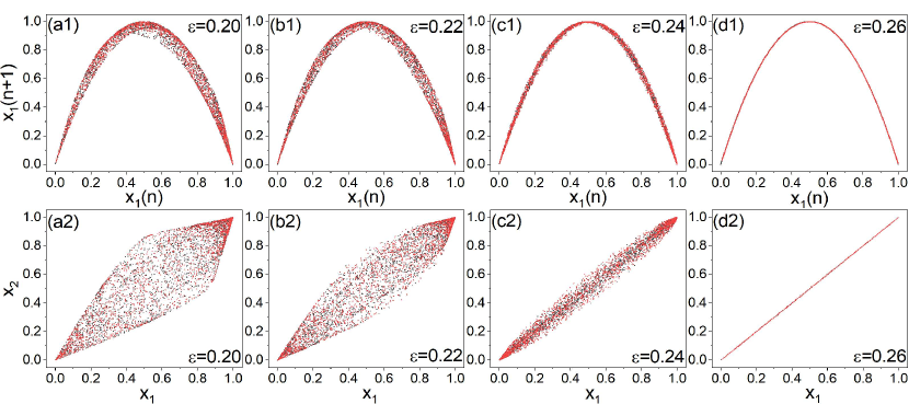
Figure 1: Predicted synchronization behavior for different values of the bifurcation parameter in coupled chaotic maps. The system consists of a pair of coupled chaotic logistic maps with coupling parameter $\varepsilon$ and respective dynamical variables $x_{1}$ and $x_{2}$. Top row (a1-d1): the predicted (black dots) and true (red dots) returned map constructed from $x_{1}$ for $\varepsilon=0.2$, 0.22, 0.24, and 0.26, respectively; bottom row (a2-d2): the predicted (black) and true (red) mutual relationship between $x_{1}$ and $x_{2}$ for the same set of parameter values, where a diagonal line represents complete synchronization.

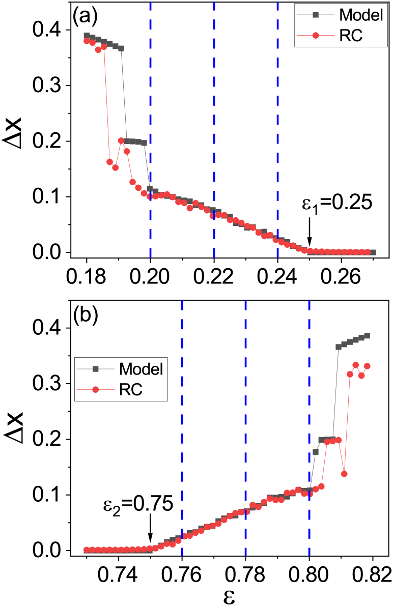
Figure 2: Predicting synchronization transition in coupled chaotic logistic maps. (a) As the coupling is strengthened, the synchronization error $\Delta x$ gradually decreases to zero at about $\varepsilon_{1}\approx 0.25$. (b) The error $\Delta x$ starts to increase from zero at about $\varepsilon_{2}\approx 0.75$. The vertical dashed lines denote the coupling parameter values used in generating the training data. The machine-predicted and true results are represented as red circles and black squares, respectively. The machine predicts correctly the transitions at both ends of the synchronization parameter regime $(\varepsilon_{1},\varepsilon_{2})$.

We consider the following system of two coupled, identical chaotic maps:

$$\mathbf{x}_{1,2}(n+1)=\mathbf{F}(\mathbf{x}_{1,2}(n))+\varepsilon[\mathbf{H}(\mathbf{x}_{2,1}(n))-\mathbf{H}(\mathbf{x}_{1,2}(n))],$$ (4)

where $\mathbf{x}_{1,2}(n)$ denote the dynamical variables of the system at the $n$th iteration, $\mathbf{F}(\mathbf{x})$ and $\mathbf{H}(\mathbf{x})$ are the map and coupling functions, respectively. As an illustrative example, we choose the one-dimensional chaotic logistic map defined on the unit interval: $F(x)=4x(1-x)$, and set the coupling function to be $H(x)=F(x)$. The critical coupling value for complete synchronization can be obtained using the master stability function Pecora and Carroll (1998); Huang et al. (2009), which gives that complete synchronization occurs for $0.25\approx\varepsilon_{1}\leq\varepsilon\leq\varepsilon_{2}\approx 0.75$.

We obtain the training data for three different values of $\varepsilon$: 0.2, 0.22 and 0.24, all in the desynchronization regime. For each $\varepsilon$ value, we collect the state variables $\{\mathbf{u}(n)\}=\{x_{1}(n),x_{2}(n)\}$ for $T=2\times 10^{3}$ successive time steps after disregarding a transient of $10^{3}$ time steps. The time series from the three values of $\varepsilon$ are combined to form a single time series which, together with the step function $\varepsilon(n)$ of the coupling parameter, are fed into the reservoir for training that yields the optimal output matrix $\mathcal{W}_{out}$. The values of the hyperparameters of the reservoir are $(D_{r},p,\sigma,\rho,\alpha,\varepsilon_{k},\varepsilon_{bias})=(100,0.2,1,10^{-5},1,1,0)$. The regression parameter for obtaining $\mathcal{W}_{out}$ is $\lambda=1\times 10^{-5}$.

To predict the synchronization transition, the trained reservoir computing machine must possess the ability to sense the change in the “synchronization climate” of the target system. Figures 1(a1-d1) show the predicted return maps (black dots) constructed from $x_{1}$ for four values of $\varepsilon$: 0.2, 0.22, 0.24, and 0.26, respectively, together with the true return maps (red dots). The corresponding plots of the mutual relation between the two maps are shown in Figs. 1(a2-d2). The first three values of $\varepsilon$ are below $\varepsilon_{1}$, so there is no synchronization, and the last value is in the synchronization regime. The reservoir machine predicts these behaviors correctly. Especially, as the value of $\varepsilon$ is increased from 0.2 to 0.26, the return map gradually evolves into the map function $F(x)=4x(1-x)$ and the points $(x_{1},x_{2})$ converges to the diagonal line, which are characteristic of complete synchronization. In fact, statistically the black and red dots cannot be distinguished, indicating the superior power of the machine to capture the collective dynamics of the target system.

Note that the first three $\varepsilon$ values (0.2, 0.22, and 0.24) are the ones used in training. It may thus not be surprising that the reservoir is able to predict correctly the distinct dynamical behaviors of the system at these parameter values, i.e., there is no synchronization. What is remarkable is that the last $\varepsilon$ value (0.26) is totally “new” to the machine as it has never been exposed to data from this parameter value, yet it predicts, still quite correctly, that there is now synchronization. This means that training at different coupling parameter values in the desynchronization regime has instilled into the machine the ability for it to “sense” the “climate” change in the collective dynamics of the target system.

As the reservoir computing has been trained to capture the “climate” of the collective dynamics in the coupled chaotic map system, it should be able to predict the synchronization transition. In particular, the expectation is that it would predict correctly the two ending points of the synchronization parameter regime $(\varepsilon_{1},\varepsilon_{2})$ at which a transition to synchronization occurs depending on the direction of parameter variation. To demonstrate the successful prediction of the transition point $\varepsilon_{1}$, we fix the output matrix $\mathcal{W}_{out}$ and increase the $\varepsilon$ value systematically from $0.18$ to $0.27$ at the step size $\Delta\varepsilon=1\times 10^{-3}$. For each $\varepsilon$ value, we let the machine generate a time series of length $T=1\times 10^{3}$ and calculate the time-averaged synchronization error $\Delta x=\left<|x_{1}-x_{2}|\right>_{T}$. Figure 2(a) shows the machine-predicted $\Delta x$ versus $\varepsilon$ (red circles), where $\Delta x$ decreases continuously for $\varepsilon\gtrsim 0.2$ and becomes zero for $\varepsilon=\varepsilon_{1}\approx 0.25$. For comparison, the true behavior of $\Delta x$ is also included in Fig. 2(a), to which the predicted result agrees well for $\varepsilon\gtrsim 0.2$. At the opposite end of the synchronization regime, the reservoir machine does an equally good job to predict the transition to synchronization at $\varepsilon_{1}\approx 0.75$ as $\varepsilon$ decreases from a larger value, as shown in Fig. 2(b), where the training data are obtained from $\varepsilon=0.76$, $0.78$ and $0.8$. The results in Fig. 2 are thus evidence that a properly trained reservoir computing machine has the power to accurately predict the critical point of transition to synchronization.

The performance of the reservoir machine in predicting the synchronization transition is affected slightly by the number and locations of the training parameter values. We find that, insofar as training is done with data from at least two distinct parameter values, the synchronization transition can be predicted. Training with data from increasingly more values of the bifurcation parameter, regardless of the order, can in general improve the prediction accuracy. Also, the closer the training parameter values to the critical point, the more accurate the prediction. (Details about the effects of the number, locations and order of the training parameter values on the prediction performance are provided in Appendix A.)

III.2 Predicting synchronization transition in coupled chaotic Lorenz oscillators

The system of a pair of coupled identical chaotic Lorenz oscillators is given by

$$\dot{x}_{1,2}=\mu(y_{1,2}-x_{1,2})+\varepsilon(x_{2,1}-x_{1,2}),$$

$$\dot{y}_{1,2}=x_{1,2}(\beta-z_{1,2})-y_{1,2}+\varepsilon(y_{2,1}-y_{1,2}),$$ (5)

$$\dot{z}_{1,2}=x_{1,2}y_{1,2}-\gamma z_{1,2}+\varepsilon(z_{2,1}-z_{1,2}),$$

where the parameter setting is $(\mu,\beta,\gamma)=(10,28,2)$ for which an isolated oscillator has a chaotic attractor Lorenz (1963). Analysis based on the master stability function gives that complete synchronization occurs for $\varepsilon>\varepsilon_{c}\approx 0.42$.

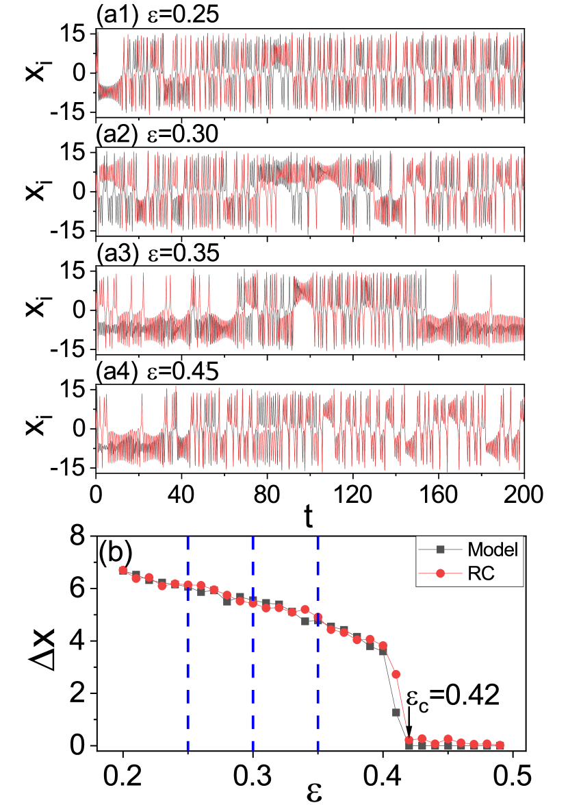
Figure 3: Predicting synchronization transition in coupled chaotic Lorenz oscillators. (a1-a3) Machine-generated time evolution of $x_{1}$ (black trace) and $x_{2}$ (red trace) for the three training values of the control parameter in the desynchronization regime: $\varepsilon=0.25$, 0.3, and 0.35. (a4) Predicted synchronization behavior for $\varepsilon=0.45$. The machine has never been exposed to data from this parameter value, yet it successfully predicts synchronization. (b) Synchronization error $\Delta x$ versus $\varepsilon$. Red circles and black squares represent the machine-predicted and true results, respectively. The three vertical dashed lines indicate the locations of the three training parameter values.

We generate the training data from three distinct values of the coupling parameter in the desynchronization regime: $\varepsilon=0.25$, $0.3$ and $0.35$. For each parameter value, a time series of length $T=4\times 10^{3}$ is collected at the time step $\Delta t=0.02$, after disregarding a transient phase of length $T_{0}=5\times 10^{3}$. The input vector $\mathbf{u}(t)\equiv[x_{1}(t),y_{1}(t),z_{1}(t),x_{2}(t),y_{2}(t),z_{2}(t)]^{T}$ and the control parameter signal $\varepsilon(t)$ are fed into the reservoir machine for training the output matrix $\mathcal{W}_{out}$. The hyperparameters of the reservoir are set as $(D_{r},p,\sigma,\rho,\alpha,\varepsilon_{k},\varepsilon_{bias})=(2\times 10^{3},0.2,0.05,0.1,1,1,0)$, and the regression parameter value is $\lambda=1\times 10^{-8}$.

Figures 3(a1-a3) show the predicted evolution of the dynamical variables $x_{1}$ and $x_{2}$ from the two oscillators for the three training parameter values preceding the onset of synchronization. The machine predicts correctly that there is no synchronization for these parameter values. When the coupling parameter value is set to be $\varepsilon=0.45$ (in the synchronization regime), the machine indeed predicts the synchronous behavior, as shown in Fig. 3(a4). To test if the machine can predict the critical transition point $\varepsilon_{c}$ for synchronization, we increase the control parameter value in the machine from $0.2$ to $0.5$ systematically and calculate the time-averaged synchronization error $\Delta x=\left<|x_{1}-x_{2}|\right>_{T}$ over a time period of $T=1\times 10^{4}$ (after discarding transients). Figure 3(b) shows $\Delta x$ versus $\varepsilon$. The machine predicted that the synchronization error approaches zero for $\varepsilon_{c}\approx 0.42$, which is in good agreement with the true value of the transition point. Similar results are obtained for alternative coupling configurations, e.g., through a single variable or a cross coupling scheme (Appendix B).

III.3 Predicting synchronization transition in coupled chaotic food-chain systems

We consider the following mutually coupled system of two food chains, each with three-species McCann and Yodzis (1994):

$$\dot{x}_{1,2} = x_{1,2}(1-\frac{x_{1,2}}{K})-\frac{a_{c}b_{c}x_{1,2}y_{1,2}}{x_{1,2}+x_{0}},$$ (6)

$$\dot{y}_{1,2} = a_{c}y_{1,2}[\frac{b_{c}x_{1,2}}{x_{1,2}+x_{0}}-1]-\frac{a_{p}b_{p}y_{1,2}z_{1,2}}{y_{1,2}+y_{0}}$$ (7)

$$+\varepsilon(y_{2,1}-y_{1,2}),$$

$$\dot{z}_{1,2} = a_{p}z_{1,2}(\frac{b_{p}y_{1,2}}{y_{1,2}+y_{0}}-1)+\varepsilon(z_{2,1}-z_{1,2}),$$ (8)

where $x_{1,2}$, $y_{1,2}$, $z_{1,2}$ are the population densities of the resource, consumer, and predator species, respectively, in each food chain. We use the parameter setting McCann and Yodzis (1994) by which each isolated food chain is a chaotic oscillator: $(K,a_{c},b_{c},a_{p},b_{p},x_{0},y_{0})=(0.99,0.4,2.009,0.08,2.876,0.16129,0.5)$. Under this setting, complete synchronization occurs for $\varepsilon>\varepsilon_{c}\approx 8.4\times 10^{-3}$.

We generate the training data from three distinct values of the coupling parameter: $\varepsilon=4.5\times 10^{-3}$, $5.5\times 10^{-3}$, and $6.5\times 10^{-3}$, all in the desynchronization regime. For each value, we generate a time series of length $T=9,600\delta t$ with $\delta t=0.5$, after disregarding the initial $T_{0}=8,000$ steps to remove any transient behavior. All six dynamical variables of the coupled system as well as the coupling strength are fed as input to the reservoir machine. The values of the hyperparameters of the reservoir machine are set as $(D_{r},p,\sigma,\rho,\alpha,\varepsilon_{k},\varepsilon_{bias})=(1000,0.695,2.30,1.20,0.27,0.049,1.53)$, where the elements of the reservoir network $\mathcal{A}$ are sampled from a standard normal distribution, and the regression parameter is $\lambda=3\times 10^{-4}$.

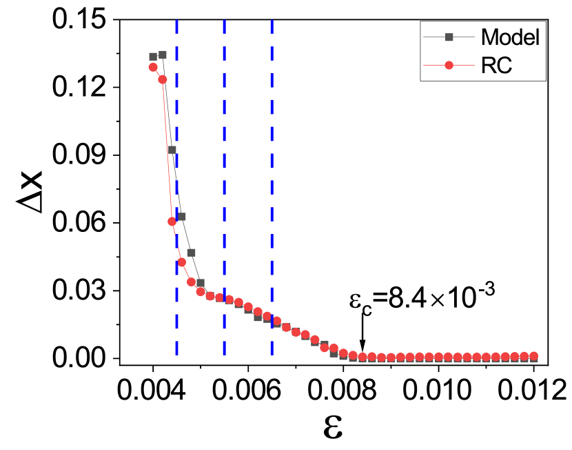
Figure 4: Predicting synchronization transition in coupled chaotic food chains. Shown are the true synchronization errors (black squares) and the reservoir’s predicted errors (red circles) for various values of the coupling strength $\varepsilon$. The three vertical blue dashed lines indicate the locations of the training parameter values.

We use the trained reservoir to predict the synchronization behaviors in the coupling range $\varepsilon\in[0.04,0.012]$, by calculating the time-averaged synchronization error $\Delta x=\left<|x_{1}-x_{2}|\right>_{T}$ over a time period of $T=2.4\times 10^{4}$ steps for each parameter value (after discarding transients with $T_{0}=4.8\times 10^{4}$ steps). Figure 4 shows that the predicted error versus $\varepsilon$ (red circles) is quite close to the true errors (black squares). The machine predicted synchronization transition point agrees with the true value well. This is quite remarkable considering that only the time series from the desynchronization regime are used as the training data.

III.4 Predicting explosive synchronization in coupled nonidentical phase oscillators

The route to complete synchronization treated in Secs. III.1, III.2, and III.3 belongs to the category of second-order phase transition, where a physical quantity characterizing the degree of synchronization varies continuously (albeit non-smoothly) through the transition point. As demonstrated, our machine learning scheme is fully capable of predicting the transition in all the cases. Another type of synchronization transition that has been extensively studied is first-order phase transition, also known as explosive synchronization Gómez-Gardeñes et al. (2011); Zou et al. (2014); Boccaletti et al. (2016), where the onset of synchronization is abrupt in the sense that the underlying characterizing quantity changes discontinuously at the transition point. The question is whether our machine learning scheme can predict explosive synchronization. Here we present an affirmative answer using the paradigmatic system in the literature Gómez-Gardeñes et al. (2011); Zou et al. (2014); Boccaletti et al. (2016) for explosive synchronization: coupled nonidentical phase oscillators.

For simplicity, we consider a small star network of $N=4$ nodes, as shown in Fig. 5(a), where the natural frequencies of the peripheral (leaf) nodes are identical and that of the hub node is proportional to its degree Zou et al. (2014). The network dynamics is described by

$$\dot{\theta}_{l}=\omega+\varepsilon\sin(\theta_{h}-\theta_{l}),$$

$$\dot{\theta}_{h}=k_{h}\omega+\varepsilon\sum_{l=1}^{3}\sin(\theta_{l}-\theta_{h}),$$ (9)

where $l=1,2,3$ denote the leaf nodes, $h$ denotes the hub node, $\varepsilon$ is the uniform coupling strength, and $k_{h}=3$ is the degree of the hub node. The degree of network synchronization can be characterized by the order parameter

$$R=\langle|\frac{1}{N}\sum^{N}_{j=1}e^{i\theta_{j}}|\rangle_{T},$$ (10)

where $j=1,\ldots,N$ is the node index, $N=4$ is the network size, $|\cdot|$ is the module function, and $\langle\cdot\rangle_{T}$ denotes the time average.

Setting $\omega=1$, we increase $\varepsilon$ systematically from $0.3$ to $0.8$, and calculate the dependence of $R$ on $\varepsilon$ by simulating Eq. (III.4). In numerical simulations, the initial conditions of the oscillators are randomly chosen from the range $(0,2\pi]$ and the integration time step is $\Delta t=0.05$. Representative numerical results are shown in Fig. 5(b) (black solid squares). It can be seen that, at about $\varepsilon_{f}=0.55$, the value of $R$ changes abruptly from about $0.45$ to about $0.9$ - the feature of a discontinuous, first-order transition. The dynamical origin of this type of explosive synchronization lies in the interplay between the heterogeneity of the network structure and dynamics, which occurs naturally in networks where the node degree and the natural frequency are positively correlated Boccaletti et al. (2016). Our goal is to use the reservoir machine trained by the time series from the desynchronization states to predict the critical coupling $\varepsilon_{f}$.

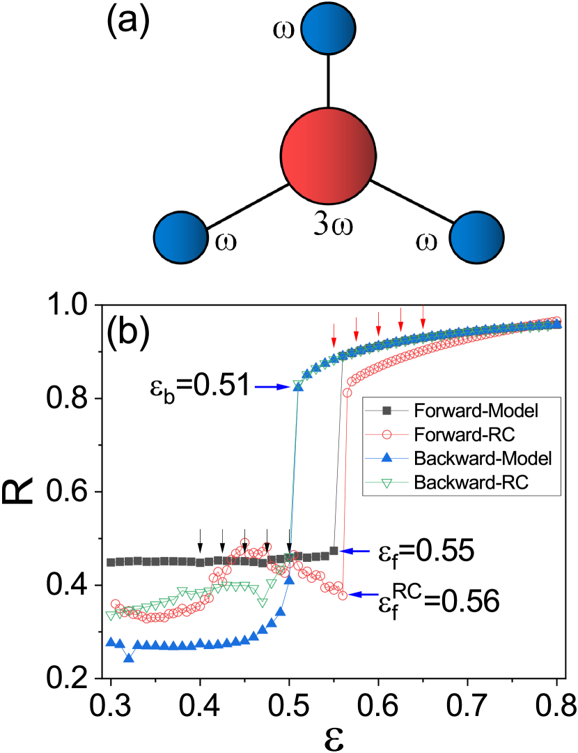
Figure 5: Predicting explosive synchronization transitions in coupled nonidentical phase oscillators. (a) A star network. (b) Synchronization order parameter $R$ versus the coupling strength $\varepsilon$ for the forward and backward transition paths. The true transitions obtained from model simulations are represented by black solid squares (forward transition) and blue solid up-triangles (backward transition). The corresponding machine predictions are displayed as red open circles (forward transition) and green empty down-triangles (backward transition). The values of the coupling parameters used to generate the training data for predicting the forward and backward transitions are marked by the black and red arrows, respectively.

The data used in training consist of time series from five values of $\varepsilon$, all inside the desynchronization regime: $\varepsilon=0.4$, $0.425$, $0.45$, $0.475$ and $0.5$. For each $\varepsilon$ value, we collect time series measurements from all nodes: $x_{j}=\sin(\theta_{j})$ and $y_{j}=\cos(\theta_{j})$. The input state vector is $\mathbf{u}=[x_{1},y_{1},x_{2},y_{2},x_{3},y_{3},x_{4},y_{4}]^{T}$, and we choose the data length to be $1.5\times 10^{4}$ that contains five segments of measurements, one from each value of $\varepsilon$. These data, together with the parameter function $\varepsilon(t)$, are fed into the machine for determining the output matrix $\mathcal{W}_{out}$. The parameters of the reservoir are $(D_{r},p,\sigma,\rho,\alpha,\varepsilon_{k},\varepsilon_{bias})=(1000,0.2,1,1.15,1,1,0)$, and the regression parameter is $\lambda=1\times 10^{-10}$.

In the predicating phase, we increase the control parameter $\varepsilon$ systematically from $0.3$ to $0.8$ with the step $\Delta\varepsilon=0.01$, and calculate from the machine output the variation of the synchronization order parameter $R$, where the output vector $\mathbf{u}=[x_{1},y_{1},x_{2},y_{2},x_{3},y_{3},x_{4},y_{4}]^{T}$ is transformed back to the original state variables $[\theta_{1},\theta_{2},\theta_{3},\theta_{4}]^{T}$ through $\theta_{i}=\arctan(y_{i}/x_{i})+\pi/2$ for $x_{i}\geq 0$ and $\theta_{i}=\arctan(y_{i}/x_{i})+\pi$ for $x_{i}<0$. The prediction results are shown in Fig. 5(b) (red open circles). It can be seen that, at about $\varepsilon^{rc}_{f}=0.56$, the value of $R$ changes suddenly from about $0.38$ to about $0.8$ - the feature of a first-order transition.

A distinct feature of explosive synchronization transitions is that when $\varepsilon$ is varied in the opposite direction, the variation of $R$ will follow a different path - the phenomenon of hysteresis Gómez-Gardeñes et al. (2011); Zou et al. (2014); Boccaletti et al. (2016). To demonstrate it, we decrease $\varepsilon$ from $0.8$ to $0.3$. To numerically observe the hysteresis in this context, we apply small random perturbations of amplitude $5\%$ to the natural frequency of the leaf nodes Zou et al. (2014). Figure 5(b) shows the results (blue solid up-triangles), where the backward and forward transition paths are identical for $\varepsilon>\varepsilon_{f}$, but diverge from each other for $\varepsilon\leq\varepsilon_{f}$. Particularly, at $\varepsilon_{f}$, we have $R\approx 0.9$ for the backward path, whereas $R\approx 0.38$ for the forward path. Along the backward path, as $\varepsilon$ decreases from $\varepsilon_{f}$, the value of $R$ maintains at large values until the critical coupling $\varepsilon_{b}\approx 0.51$, where $R$ is suddenly decreased from about $0.8$ to about $0.4$. Since $\varepsilon_{b}<\varepsilon_{f}$, a hysteresis loop of width $\Delta\varepsilon\equiv\varepsilon_{f}-\varepsilon_{b}$ emerges in the parameter region $\varepsilon\in(\varepsilon_{b},\varepsilon_{f})$. The dynamical mechanism for the hysteresis loop is the bistability of the synchronization manifold in this region, deemed as a necessary condition for generating a first-order phase transition Boccaletti et al. (2016).

To predict the backward transition path, we use five values of the coupling parameter in the strong synchronization regime to obtain the training data: $\varepsilon=0.65$, $0.625$, $0.6$, $0.575$ and $0.55$. The input vector is constructed in the same way as for predicting the forward transition, and the hyperparameter values are $(D_{r},p,\sigma,\rho)=(1\times 10^{3},0.2,1,1.15)$ and the regression parameter is $\lambda=1\times 10^{-7}$. We decrease $\varepsilon$ systematically from $0.8$ to $0.3$. The dependence of $R$ on $\varepsilon$ predicted by the machine is shown in Fig. 5(b) (open green down-triangles). It can be seen that the machine predictions agree well with the true behavior of the backward transition where, at the transition point $\varepsilon_{b}$, the value of $R$ decreases suddenly from about 0.8 to about 0.45.

IV Discussion

We have articulated and tested a model-free, machine learning scheme to predict the synchronization transition in systems of coupled oscillators. The machine is trained with time series collected from a small number of the coupling (control) parameter, all in the desynchronization regime, as well as the value of the control parameter itself through a specially designed input channel. Prediction is achieved by feeding any desired parameter value into the input parameter channel. A properly trained machine is able to not only reproduce, statistically, the nature of the collective dynamics at the training parameter values, but also predict, quantitatively, how the collective dynamics change with respect to the variations in the control parameter. Examples demonstrating the predictive power of our machine learning scheme include complete synchronization in coupled identical chaotic oscillators and explosive synchronization in coupled nonidentical phase oscillators. For complete synchronization, both the critical coupling for synchronization and the variation in the degree of synchronization about the critical point can be well predicted. For explosive synchronization, our scheme not only predicts the forward and backward critical couplings, but also reproduces the hysteresis loop associated with a first-order transition. Due to the importance of synchronization to the functionality and operation in many natural and man-made systems, our machine learning method may find broad applications.

Reservoir computing based prediction of chaotic systems is an extremely active field of research at the boundary between nonlinear dynamics and machine learning Lipton et al. (2015); Haynes et al. (2015); Larger et al. (2017); Pathak et al. (2017); Lu et al. (2017); Duriez et al. (2017); Lu et al. (2018); Pathak et al. (2018a, b); Carroll (2018); Nakai and Saiki (2018); Zimmermann and Parlitz (2018); Weng et al. (2019); Griffith et al. (2019); Jiang and Lai (2019); Vlachas et al. (2019); Fan et al. (2020); Zhang et al. (2020); Guo et al. (2021). The main contribution of the present work is the development of a reservoir computing scheme to predict or anticipate synchronization in systems of coupled nonlinear oscillators. Our work focuses on predicting the collective dynamics instead of the state evolution, based on the general idea to view the predictive power of reservoir computing as a kind of ability to replicate the dynamical “climate” of the target system Pathak et al. (2017), which is gained through training with time series data. Inspired by the recent works on conducting training at multiple parameter values to predict bifurcations Cestnik and Abel (2019); Kong et al. (2021), our work adopts a similar method by training the machine at a small number of control parameter values in the desynchronization regime to instill into the machine the ability to sense the change in the “synchronization climate” with the control parameter. With the desired (arbitrary) value of the control parameter fed into the input parameter channel, a well trained reservoir computing machine is then able to accurately predict the critical transition between desynchronization and synchronization, regardless of the nature of the underlying transition, e.g., second-order or first-order.

The type of collective dynamics tested in the present work is complete synchronization between a pair of coupled chaotic oscillators for which the transition is of the nature of second order, and the first order, explosive synchronization in a small network. To extend our work to other types of collective dynamics in large complex systems, such as partial (cluster) synchronization, chimera-like states and spiral waves, is worth pursuing. A difficulty with large systems is the requirement to use large reservoir networks so that the complexity of the machine can “overpower” that of the target system. Quantitatively, how the size of the reservoir network should be enlarged to accommodate an increase in the size of the target system as characterized by, e.g., a scaling law, remains unknown at the present. With the use of large reservoir networks come the issues of data requirement and computation overload, as to train a large reservoir machine not only requires massive data but also imposes a serious demand for the computational resource. One approach to deal with this difficulty is the parallel reservoir computing scheme Pathak et al. (2018b); Zimmermann and Parlitz (2018). However, a recent work revealed that the parallel scheme may fail to sense and predict the phase coherence among a pair of coupled, nonidentical chaotic oscillators Zhang et al. (2020). It remains a worthy issue to study if the parallel scheme can be exploited to predict the collective dynamics among a large number of coupled oscillators.

Appendix A Robustness of reservoir computing scheme for predicting synchronization transition

A.1 Effect of nonuniform training data on predication performance

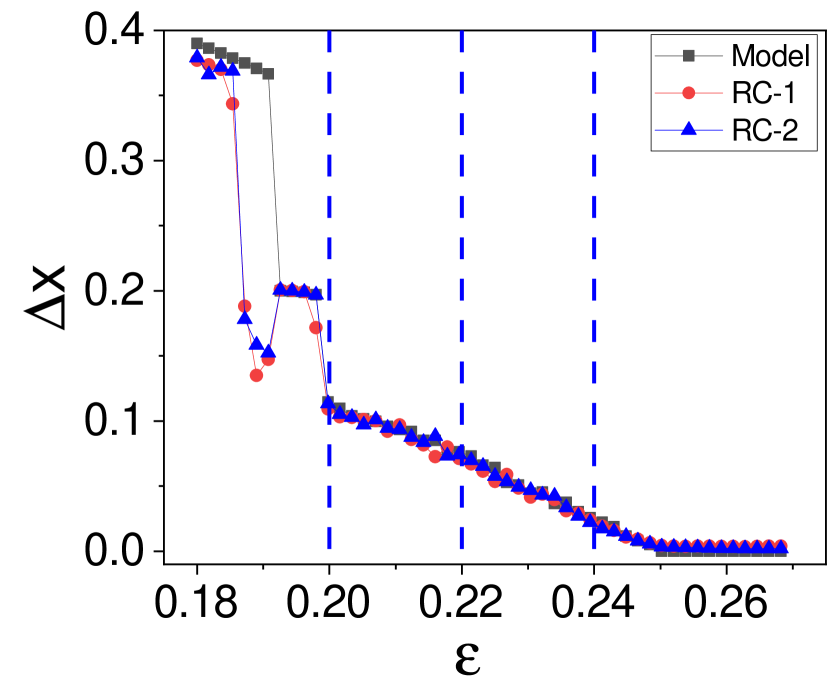
Figure 6: Effect of nonuniform segment length on predication performance. Shown is the variation of the synchronization error $\Delta x$ versus the coupling parameter $\varepsilon$ for the system of coupled chaotic logistic maps in the main text. The parameter values are the same as those in Fig. 2(a) in the main text, but with nonuniform length of the time series for different values of the training parameter. Red discs: $T=1000$, $2000$ and $3000$ for $\varepsilon=0.2$, $0.22$ and $0.24$, respectively; blue triangles: $T=3000$, $2000$ and $1000$ for $\varepsilon=0.2$, $0.22$ and $0.24$, respectively. The black squares denote the corresponding results from the target system. The vertical dashed lines denote the values of the control parameter for training.

In the main text, the lengths of the time series for training at different values of the control parameter are identical. For example, for the system of a pair of chaotic logistic maps in Sec. IIIA, the length of the time series is $T=2\times 10^{3}$. If time series of nonuniform length are used for training, the predication performance will be not affected. To demonstrate this, we calculate the machine predicted synchronization error versus the coupling parameter using training time series of length $T=1000$, $2000$ and $3000$ for $\varepsilon=0.2$, $0.22$ and $0.24$, respectively, as shown in Fig. 6 (red discs). Comparing with the results of from direct model simulations (black squares), we see that the reservoir machine still predicts well the transition about the critical point. Similar results are also obtained when the training data have the length $T=3000$ for $\varepsilon=0.20$, $2000$ for $\varepsilon=0.22$, and $1000$ for $\varepsilon=0.24$, as shown by the blue triangles in Fig. 6. The observation is that, insofar as the training data set is sufficient (e.g., $>1000$), both the critical point and the associated transition behavior can be well predicted.

A.2 Effect of order of training at different control parameter values on predication performance

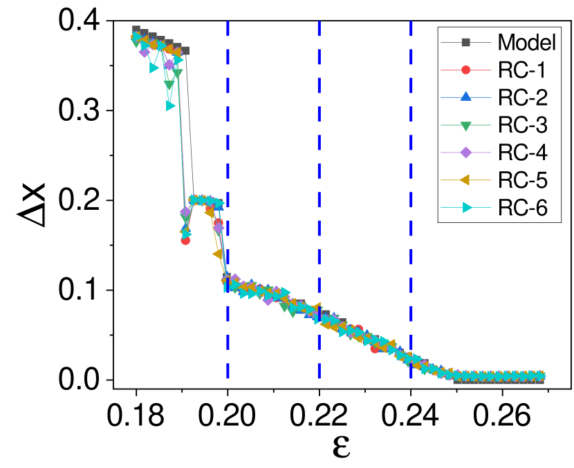
Figure 7: Effect of the order of training at different control parameter values on predication performance. The model and parameters are identical to those in Fig. 2(a) in the main text, while the order of training at the three values of the control parameter ($\varepsilon=0.2$, $0.22$ and $0.24$, as indicated by the vertical dashed lines) is altered. Shown is the synchronization error $\Delta x$ versus $\varepsilon$. A change in the training order has little effect on the performance.

In our machine learning scheme, the training data are generated by combining the time series acquired from different values of the control parameter. We find that order of training at these parameter values does not affect the the predication performance. To demonstrate this, we use the results in Fig. 2(a) in the main text as a reference and obtain prediction results for altered training orders. Since data are obtained from three values of the control parameter $\varepsilon$ (0.2, 0.22, and 0.24), there are six distinct sequences of training order. Figure 7 shows the machine predicted synchronization error $\Delta x$ versus $\varepsilon$ for all six cases, together with the true results obtained from direct simulation of the target system. It can be seen that different orders of training lead to essentially the same result. A heuristic reason is that, in obtaining the output matrix $\mathbf{W}_{out}$, the regression operation is conducted for the entire, combined time series. For a linear regression, the orders by which the time series are combined have little effect on the result.

A.3 Impact of training control parameter values on predication performance

Figure 8: Impact of training control parameter values on predication performance. With the model for Fig. 2(a) in the main text, the values of the control parameter for training ($\varepsilon=0.2$, $0.22$ and $0.24$) are shifted by a small amount toward the critical point $\varepsilon_{1}=0.25$. Shown is the predication error $\langle\Delta x_{e}\rangle$ versus the parameter value for training, denoted as $\varepsilon_{M}$. As the training parameter values move closer to the critical point (decreasing $\varepsilon_{M}$), the predication performance is continuously improved.

For the given number of training parameter values, the closer they are to the transition point, the better the predication performance will be. To demonstrate this, we consider the system of coupled chaotic Logistic maps in the main text and test the predication performance by changing the values of $\varepsilon$ to $\varepsilon_{M}-0.04$, $\varepsilon_{M}-0.02$ and $\varepsilon_{M}$, where $\varepsilon_{M}$ is below the synchronization transition point so that all three parameter values are still in the desynchronization regime. We define the following prediction error about the transition as

$$\langle\Delta x_{e}\rangle=\langle|\Delta\hat{x}(\varepsilon)-\Delta x(\varepsilon)|\rangle,$$

where $\Delta\hat{x}(\varepsilon)$ and $\Delta x(\varepsilon)$ are the synchronization errors obtained from model simulation and machine outputs, and $\langle\ldots\rangle$ denotes that the results are averaged over the range $0.245\leq\varepsilon\leq 0.255$. Figure 8 shows $\langle\Delta x_{e}\rangle$ versus $\varepsilon_{M}$, the largest training parameter value chosen in the desynchronization regime. As $\varepsilon_{M}$ approaches the critical point, the error $\langle\Delta x_{e}\rangle$ decreases continuously, indicating that choosing the training parameter values closer to the critical point can improve the prediction.

A.4 Impact of the number of training parameter values on predication performance

Figure 9: Impact of the number of training parameter values on predication performance. The model and parameter values are identical to those in Fig. 2(a) in the main text, except that the number $m$ of control parameter values chosen to obtain the time series data for training now varies. Shown is the predication error $\langle\Delta x_{e}\rangle$ versus $m$. An increase in $m$ above three improves the predication performance but only slightly, indicating that the reservoir computing machine is already able to capture the dynamical “climate” of the target system with training conducted at three values of the control parameter.

Increasing the number $m$ of control parameter values in the desynchronization regime for training can in general improve the prediction performance, but only incrementally, insofar as training is conducted based on time series data collected from at least two values of the control parameter. To demonstrate this, we take the model in Fig. 2(a) in the main text and investigate how the value of $m$ impacts the predicted synchronization error, For simplicity, we choose the $m$ training parameter values from the interval $[0.20,0.24]$ (including the two ending points). Figure 9 shows $\langle\Delta x_{e}\rangle$ versus $m$. As the value of $m$ increases from $2$ to $4$, the predication error is reduced but the trend slows down for $m>4$, indicating that it is generally not necessary to conduct the training for more than three or four values of the control parameter.

Appendix B Alternative types of coupling functions

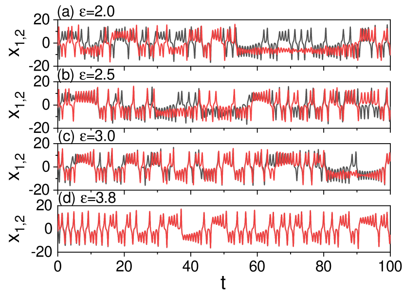
Figure 10: Predicting collective dynamical behaviors arising from the system of two coupled Lorenz chaotic oscillators under the $x$ coupling scheme. Shown is the time evolution of the reservoir outputs $x_{1}$ (black curve) and $x_{2}$ (red curve) for different values of the control parameter: (a) $\varepsilon=2.0$, (b) $\varepsilon=2.5$, (c) $\varepsilon=3.0$, and (d) $\varepsilon=3.8$. There is no synchronization in the first three cases, but there is for the last case, in agreement with the result of the analysis based on the master stability function that the oscillators are completely synchronized for $\varepsilon>\varepsilon_{c}=3.7$.

The coupling function can play a role in the synchronization dynamics: changing the function can alter the synchronization type and the critical point. In the main text, we treat the relatively simple setting of diagonal coupling function, i.e., all the dynamical variables of the oscillators are diffusively coupled. To test if the machine learning scheme remains effective for alternative types of coupling functions, we take the model of coupled chaotic Lorenz oscillators studied in the main text [Fig. 3(a)] and evaluate the prediction performance with different coupling functions.

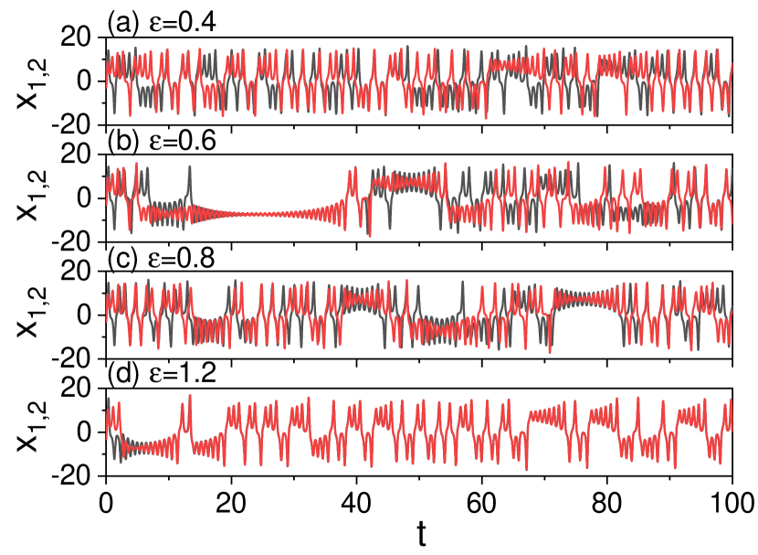
Figure 11: Predicting collective dynamical behaviors arising from the system of two coupled Lorenz chaotic oscillators under the $y$ coupling scheme. Legends are the same as those in Fig. 10. For (a) $\varepsilon=0.4$, (b) $\varepsilon=0.6$, (c) $\varepsilon=0.8$, there is no synchronization, but complete synchronization occurs for (d) $\varepsilon=1.2$, in agreement with the prediction of the theoretical analysis that the oscillators should be completely synchronized for $\varepsilon>\varepsilon_{c}=3.7$.

When the oscillators are coupled through the variable $x$ of the Lorenz oscillator, the system equations are

$$\dot{x}_{1,2}=\alpha(y_{1,2}-x_{1,2})+\varepsilon(x_{2,1}-x_{1,2}),$$

$$\dot{y}_{1,2}=x_{1,2}(\beta-z_{1,2})-y_{1,2},$$ (11)

$$\dot{z}_{1,2}=x_{1,2}y_{1,2}-\gamma z_{1,2}.$$

We use the same parameter values as in the main text. An analysis of the master stability function reveals that, for this alternative coupling scheme, the two oscillators will be completely synchronized for $\varepsilon>\varepsilon_{c}\approx 3.7$. To generate the training data, we collect time series from three values of the control parameter: $\varepsilon=2.0$, $2.5$ and $3.0$. The parameters of the reservoir are $(D_{r},p,\sigma,\rho,\alpha,\varepsilon_{k},\varepsilon)=(2\times 10^{3},0.2,0.05,1\times 10^{-3},1,1,0)$ and the regression parameter is $\lambda=10^{-7}$. Fig. 10 shows the prediction result, where the machine output variables $x_{1}$ and $x_{2}$ are not synchronized for $\varepsilon=2.0$, 2.5, and 3.0 [Figs. 10(a-c), respectively], but are synchronized for $\varepsilon=3.8$ [Fig. 10(d)], in complete agreement with the theoretical analysis.

We next consider the scheme by which the $y$ variables of the oscillators are coupled. The system equations are

$$\dot{x}_{1,2}=\alpha(y_{1,2}-x_{1,2}),$$

$$\dot{y}_{1,2}=x_{1,2}(\beta-z_{1,2})-y_{1,2}+\varepsilon(y_{2,1}-y_{1,2}),$$ (12)

$$\dot{z}_{1,2}=x_{1,2}y_{1,2}-\gamma z_{1,2},$$

where the two oscillators are completely synchronized for $\varepsilon>\varepsilon_{c}\approx 1.1$, as predicated by the master stability function. We train the reservoir machine based on data from $\varepsilon=0.4$, $0.6$ and 0.8. The parameter values of the reservoir are the same as for Figs. 10(a-d), but the regression parameter is $\lambda=10^{-10}$. Figure 11 shows the predicted synchronization behavior between the machine outputs $x_{1}$ and $x_{2}$ for different values of the control parameter. In complete agreement with the result of the theoretical analysis, there is no synchronization for $\varepsilon=0.4$, 0.6, and 0.8 [Figs. 11(a-c), respectively], but the machine output variables are synchronized for $\varepsilon=1.2>\varepsilon_{c}$, as shown in Fig. 11(d).

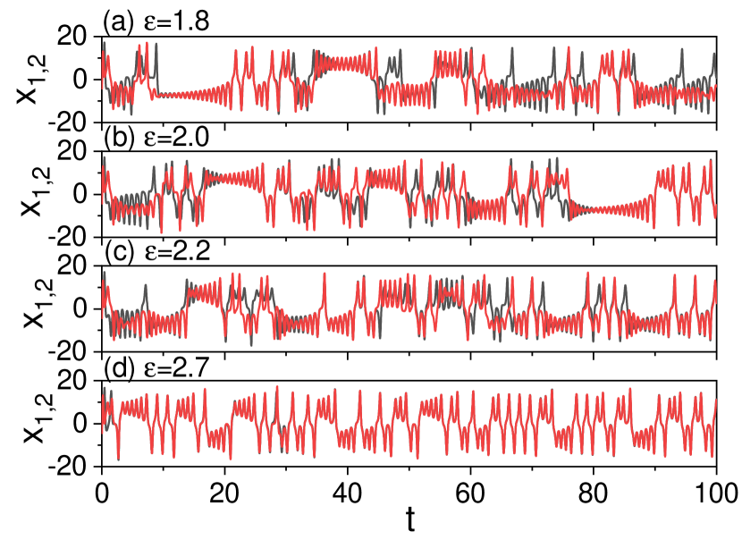
Figure 12: Predicting collective dynamical behaviors arising from the system of two coupled Lorenz chaotic oscillators under the cross coupling scheme. Legends are the same as those in Fig. 10. For (a) $\varepsilon=1.8$, (b) $\varepsilon=2.0$, (c) $\varepsilon=2.28$, there is no synchronization, but complete synchronization occurs for (d) $\varepsilon=2.7$, in agreement with the prediction of the theoretical analysis that the oscillators should be completely synchronized for $\varepsilon>\varepsilon_{c}=2.6$.

We finally consider the cross coupling scheme, i.e., variable $x$ of one oscillator is coupled to variable $y$ of the other. The system is described by

$$\dot{x}_{1,2}=\alpha(y_{1,2}-x_{1,2}),$$

$$\dot{y}_{1,2}=x_{1,2}(\beta-z_{1,2})-y_{1,2}+\varepsilon(x_{2,1}-x_{1,2}),$$ (13)

$$\dot{z}_{1,2}=x_{1,2}y_{1,2}-\gamma z_{1,2}.$$

For this coupling scheme, according to the theoretical analysis, the two oscillators are completely synchronized for $\varepsilon>\varepsilon_{c}\approx 2.6$. Training data are generated for $\varepsilon=1.8$, $2.0$ and $2.2$, all in the desynchronization regime. The values of the hyperparameters of the reservoir and of the regression parameter are the same as those in Fig. 11. Figure 12 shows the predicted synchronization behavior between the reservoir outputs $x_{1}$ and $x_{2}$ for different values of $\varepsilon$. There is no synchronization for $\varepsilon=1.8$, 2.0, and 2.2, as shown in Fig. 12(a-c), respectively, but for $\varepsilon=2.7>\varepsilon_{c}$, the machine predicts synchronization, as shown in Fig. 12(d). These machine predicted behaviors are in full agreement with the result of the theoretical analysis.

References

- Kuramoto (1984) Y. Kuramoto, Chemical Oscillations, Waves, and Turbulence (Springer, Berlin, 1984).
- Pikovsky et al. (2003) A. Pikovsky, M. Rosenblum, and J. Kurths, Synchronization: A Universal Concept in Nonlinear Science (Cambridge University Press, Cambridge, 2003).
- Strogatz (2003) S. H. Strogatz, Sync: The Emerging Science of Spontaneous Order (Hyperion, New York, 2003).
- Pecora and Carroll (1990) L. M. Pecora and T. L. Carroll, “Synchronization in chaotic systems,” Phys. Rev. Lett. 64, 821 (1990).
- Rosenblum et al. (1996) M. G. Rosenblum, A. S. Pikovsky, and J. Kurths, “Phase synchronization of chaotic oscillators,” Phys. Rev. Lett. 76, 1804 (1996).
- Kocarev and Parlitz (1996) L. Kocarev and U. Parlitz, “Generalized synchronization, predictability, and equivalence of unidirectionally coupled dynamical systems,” Phys. Rev. Lett. 76, 1816 (1996).
- Kandel et al. (1991) E. R. Kandel, J. H. Schwartz, and T. M. Jessell, Principle of Neural Science, 3rd ed. (Appleton and Lange, Norwalk CT, 1991).
- Lai et al. (2006) Y.-C. Lai, M. G. Frei, and I. Osorio, “Detecting and characterizing phase synchronization in nonstationary dynamical systems,” Phys. Rev. E 73, 026214 (2006).
- Lai et al. (2007) Y.-C. Lai, M. G. Frei, I. Osorio, and L. Huang, “Characterization of synchrony with applications to epileptic brain signals,” Phys. Rev. Lett. 98, 108102 (2007).
- Osorio and Lai (2011) I. Osorio and Y.-C. Lai, “A phase-synchronization and random-matrix based approach to multichannel time-series analysis with application to epilepsy,” Chaos 21, 033108 (2011).
- Jaeger (2001) H. Jaeger, “The “echo state” approach to analysing and training recurrent neural networks-with an erratum note,” Bonn, Germany: German National Research Center for Information Technology GMD Technical Report 148, 13 (2001).
- Jaeger and Haas (2004) H. Jaeger and H. Haas, “Harnessing nonlinearity: Predicting chaotic systems and saving energy in wireless communication,” Science 304, 78 (2004).
- Pecora and Carroll (1998) L. M. Pecora and T. L. Carroll, “Master stability functions for synchronized coupled systems,” Phys. Rev. Lett. 80, 2109 (1998).
- Huang et al. (2009) L. Huang, Q. Chen, Y.-C. Lai, and L. M. Pecora, “Generic behavior of master-stability functions in coupled nonlinear dynamical systems,” Phys. Rev. E 80, 036204 (2009).
- Watanabe and Strogatz (1993) S. Watanabe and S. H. Strogatz, “Integrability of a globally coupled oscillator array,” Phys. Rev. Lett. 70, 2391 (1993).
- Ott and Antonsen (2008) E. Ott and T. M. Antonsen, “Low dimensional behavior of large systems of globally coupled oscillators,” Chaos 18, 037113 (2008).
- Williams et al. (2013a) C. R. S. Williams, T. E. Murphy, R. Roy, F. Sorrentino, T. Dahms, and E. Schöll, “Experimental observations of group synchrony in a system of chaotic optoelectronic oscillators,” Phys. Rev. Lett. 110, 064104 (2013a).
- Williams et al. (2013b) C. Williams, F. Sorrentino, T. E. Murphy, and R. Roy, “Synchronization states and multistability in a ring of periodic oscillators: Experimentally variable coupling delays,” Chaos 23, 143117 (2013b).
- Hart et al. (2015) J. D. Hart, J. P. Pade, T. Pereira, T. E. Murphy, and R. Roy, “Adding connections can hinder network synchronization of time-delayed oscillators,” Phys. Rev. E 92, 022804 (2015).
- Arenas et al. (2008) A. Arenas, A. Díaz-Guilera, J. Kurths, Y. Moreno, and C. S. Zhou, “Synchronization in complex networks,” Phy. Rep. 469, 93 (2008).
- Barahona and Pecora (2002) M. Barahona and L. M. Pecora, “Synchronization in small-world systems,” Phys. Rev. Lett. 89, 054101 (2002).
- Nishikawa et al. (2003) T. Nishikawa, A. E. Motter, Y.-C. Lai, and F. C. Hoppensteadt, “Heterogeneity in oscillator networks: Are smaller worlds easier to synchronize?” Phys. Rev. Lett. 91, 014101 (2003).
- Wang et al. (2007) X. G. Wang, Y.-C. Lai, and C. H. Lai, “Enhancing synchronization based on complex gradient networks,” Phys. Rev. E 75, 056205 (2007).
- Ricci et al. (2012) F. Ricci, R. Tonelli, L. Huang, and Y.-C. Lai, “Onset of chaotic phase synchronization in complex networks of coupled heterogeneous oscillators,” Phys. Rev. E 86, 027201 (2012).
- Pecora et al. (2014) L. M. Pecora, F. Sorrentino, A. M. Hagerstrom, T. E. Murphy, and R. Roy, “Cluster synchronization and isolated desynchronization in complex networks with symmetries,” Nat. Commun. 5, 4079 (2014).
- Sorrentino et al. (2016) F. Sorrentino, L. M. Pecora, A. M. Hagerstrom, T. E. Murphy, and R. Roy, “Cluster synchronization and isolated desynchronization in complex networks with symmetries,” Sci. Adv. 2, e1501737 (2016).
- Gómez-Gardeñes et al. (2011) J. Gómez-Gardeñes, S. Gómez, A. Arenas, and Y. Moreno, “Explosive synchronization transitions in scale-free networks,” Phys. Rev. Lett. 106, 128701 (2011).
- Zou et al. (2014) Y. Zou, T. Pereira, M. Small, Z. Liu, and J. Kurths, “Basin of attraction determines hysteresis in explosive synchronization,” Phys. Rev. Lett. 112, 114102 (2014).
- Boccaletti et al. (2016) S. Boccaletti, J. A. Almendral, S. Guan, I. Leyva, Z. Liu, I. Sendiña-Nadal, Z. Wang, and Y. Zou, “Explosive transitions in complex networks’ structure and dynamics: Percolation and synchronization,” Phys. Rep. 660, 1 (2016).
- Lipton et al. (2015) Z. C. Lipton, J. Berkowitz, and C. Elkan, “A critical review of recurrent neural networks for sequence learning,” arXiv:1506.00019 (2015).
- Haynes et al. (2015) N. D. Haynes, M. C. Soriano, D. P. Rosin, I. Fischer, and D. J. Gauthier, “Reservoir computing with a single time-delay autonomous Boolean node,” Phys. Rev. E 91, 020801 (2015).
- Larger et al. (2017) L. Larger, A. Baylón-Fuentes, R. Martinenghi, V. S. Udaltsov, Y. K. Chembo, and M. Jacquot, “High-speed photonic reservoir computing using a time-delay-based architecture: Million words per second classification,” Phys. Rev. X 7, 011015 (2017).
- Pathak et al. (2017) J. Pathak, Z. Lu, B. R. Hunt, M. Girvan, and E. Ott, “Using machine learning to replicate chaotic attractors and calculate lyapunov exponents from data,” Chaos 27, 121102 (2017).
- Lu et al. (2017) Z. Lu, J. Pathak, B. Hunt, M. Girvan, R. Brockett, and E. Ott, “Reservoir observers: Model-free inference of unmeasured variables in chaotic systems,” Chaos 27, 041102 (2017).
- Duriez et al. (2017) T. Duriez, S. L. Brunton, and B. R. Noack, Machine Learning Control-Taming Nonlinear Dynamics and Turbulence (Springer, 2017).
- Lu et al. (2018) Z. Lu, B. R. Hunt, and E. Ott, “Attractor reconstruction by machine learning,” Chaos 28, 061104 (2018).
- Pathak et al. (2018a) J. Pathak, A. Wilner, R. Fussell, S. Chandra, B. Hunt, M. Girvan, Z. Lu, and E. Ott, “Hybrid forecasting of chaotic processes: Using machine learning in conjunction with a knowledge-based model,” Chaos 28, 041101 (2018a).
- Pathak et al. (2018b) J. Pathak, B. Hunt, M. Girvan, Z. Lu, and E. Ott, “Model-free prediction of large spatiotemporally chaotic systems from data: A reservoir computing approach,” Phys. Rev. Lett. 120, 024102 (2018b).
- Carroll (2018) T. L. Carroll, “Using reservoir computers to distinguish chaotic signals,” Phys. Rev. E 98, 052209 (2018).
- Nakai and Saiki (2018) K. Nakai and Y. Saiki, “Machine-learning inference of fluid variables from data using reservoir computing,” Phys. Rev. E 98, 023111 (2018).
- Zimmermann and Parlitz (2018) R. S. Zimmermann and U. Parlitz, “Observing spatio-temporal dynamics of excitable media using reservoir computing,” Chaos 28, 043118 (2018).
- Weng et al. (2019) T. Weng, H. Yang, C. Gu, J. Zhang, and M. Small, “Synchronization of chaotic systems and their machine-learning models,” Phys. Rev. E 99, 042203 (2019).
- Griffith et al. (2019) A. Griffith, A. Pomerance, and D. J. Gauthier, “Forecasting chaotic systems with very low connectivity reservoir computers,” Chaos 29, 123108 (2019).
- Jiang and Lai (2019) J. Jiang and Y.-C. Lai, “Model-free prediction of spatiotemporal dynamical systems with recurrent neural networks: Role of network spectral radius,” Phys. Rev. Research 1, 033056 (2019).
- Vlachas et al. (2019) P. R. Vlachas, J. Pathak, B. R. Hunt, T. P. Sapsis, M. Girvan, E. Ott, and P. Koumoutsakos, “Forecasting of spatio-temporal chaotic dynamics with recurrent neural networks: A comparative study of reservoir computing and backpropagation algorithms,” arXiv preprint arXiv:1910.05266 (2019).
- Fan et al. (2020) H. Fan, J. Jiang, C. Zhang, X. Wang, and Y.-C. Lai, “Long-term prediction of chaotic systems with machine learning,” Phys. Rev. Research 2, 012080 (2020).
- Zhang et al. (2020) C. Zhang, J. Jiang, S.-X. Qu, and Y.-C. Lai, “Predicting phase and sensing phase coherence in chaotic systems with machine learning,” Chaos 30, 083114 (2020).
- Guo et al. (2021) Y. Guo, H. Zhang, L. Wang, H. Fan, J. Xiao, and X. Wang, “Transfer learning of chaotic systems,” Chaos 31, 011104 (2021).
- Cestnik and Abel (2019) R. Cestnik and M. Abel, “Inferring the dynamics of oscillatory systems using recurrent neural networks,” Chaos 29, 063128 (2019).
- Kong et al. (2021) L.-W. Kong, H.-W. Fan, C. Grebogi, and Y.-C. Lai, “Machine learning prediction of critical transition and system collapse,” Phys. Rev. Research 3, 013090 (2021).
- Wang et al. (2011a) W.-X. Wang, R. Yang, Y.-C. Lai, V. Kovanis, and C. Grebogi, “Predicting catastrophes in nonlinear dynamical systems by compressive sensing,” Phys. Rev. Lett. 106, 154101 (2011a).
- Wang et al. (2011b) W.-X. Wang, R. Yang, Y.-C. Lai, V. Kovanis, and M. A. F. Harrison, “Time-series-based prediction of complex oscillator networks via compressive sensing,” EPL (Europhys. Lett.) 94, 48006 (2011b).
- Wang et al. (2016) W. Wang, Y.-C. Lai, and C. Grebogi, “Data based identification and prediction of nonlinear and complex dynamical systems,” Phys. Rep. 644, 1 (2016).
- Su et al. (2012) R.-Q. Su, X. Ni, W.-X. Wang, and Y.-C. Lai, “Forecasting synchronizability of complex networks from data,” Phys. Rev. E 85, 056220 (2012).
- Lorenz (1963) E. N. Lorenz, “Deterministic nonperiodic flow,” J. Atmos. Sci. 20, 130 (1963).
- McCann and Yodzis (1994) K. McCann and P. Yodzis, “Nonlinear dynamics and population disappearances,” Ame. Naturalist 144, 873 (1994).