Polymer translocation into cavities: Effects of confinement geometry, crowding and bending rigidity on the free energy

Abstract

Monte Carlo simulations are used to study the translocation of a polymer into a cavity. Modeling the polymer as a hard-sphere chain with a length up to $N$=601 monomers, we use a multiple-histogram method to measure the variation of the conformational free energy of the polymer with respect to the number of translocated monomers. The resulting free-energy functions are then used to obtain the confinement free energy for the translocated portion of the polymer. We characterize the confinement free energy for a flexible polymer in cavities with constant cross-sectional area $A$ for various cavity shapes (cylindrical, rectangular and triangular) as well as for tapered cavities with pyramidal and conical shape. The scaling of the free energy with cavity volume and translocated polymer subchain length is generally consistent with predictions from simple scaling arguments, with small deviations in the scaling exponents likely due to finite-size effects. The confinement free energy depends strongly on cavity shape anisometry and is a minimum for an isometric cavity shape with a length/width ratio of unity. Entropic depletion at the edges or vertices of the confining cavity are evident in the results for constant-$A$ and pyramidal cavities. For translocation into infinitely long cones, the scaling of the free energy with taper angle is consistent with a theoretical prediction employing the blob model. We also examine the effects of polymer bending rigidity on the translocation free energy for cylindrical cavities. For isometric cavities, the observed scaling behaviour is in partial agreement with theoretical predictions, with discrepancies arising from finite-size effects that prevent the emergence of well-defined scaling regimes. In addition, translocation into highly anisometric cylindrical cavities leads to a multi-stage folding process for stiff polymers. Finally, we examine the effects of crowding agents inside the cavity. We find that the confinement free energy increases with crowder density. At constant packing fraction the magnitude of this effect lessens with increasing crowder size for crowder/monomer size ratio $\geq 1$.

I Introduction

The equilibrium conformational behaviour of polymers confined to small spaces has been the subject of much theoretical interest for decades.Daoud and De Gennes (1977); de Gennes (1979) The basic concept is straightforward: if one or more confinement dimensions is smaller than the mean size of the polymer, the number of accessible conformations is significantly reduced. This results a reduction in the conformational entropy and to an increase in the free energy of the polymer relative to its unconfined state. In spite of this apparent simplicity, theoretical and computational studies have revealed a wide variety of scaling regimes for polymers confined to channelsDai et al. (2016) and cavities.Gao et al. (2014); Sakaue (2018, 2007) Although the precise scaling behaviour is dependent on just a few system properties such as the confinement dimensions and the polymer contour length and bending rigidity, new regimes continue to be discovered.Hayase et al. (2017) These theoretical studies have been complemented by progress in the experiment realm, where recent advances in nanofabrication techniques have enabled the study of DNA (deoxyribonucleic acid) confined to narrow channelsReisner et al. (2012) and cavities.Langecker et al. (2011); Liu et al. (2015); Sampath (2016); Cadinu et al. (2017, 2018); Zhang et al. (2018) In addition, some experimental studies have examined more complex confinement behaviour for cases where individual DNA molecules are distributed among many cavities connected by nanoporesNykypanchuk et al. (2002) or by narrow slits between confining surfaces.Klotz et al. (2015a, b) The insights provided by these experimental and theoretical studies are expected to benefit the development of nanofluidic technologies for the manipulation and analysis of DNA and other biopolymers.

Confinement is a relevant factor in many examples of polymer translocation through nanopores.Muthukumar (2011) For example, many biological phenomena such as viral DNA packaging or ejection, transport of messenger RNA (ribonucleic acid) across the nuclear pore complex and horizontal gene transfer between bacteria involve translocation into or out of a confined or otherwise crowded environment.Alberts et al. (2008); Lodish et al. (2012) In addition, some recently developed experimental techniques for studying translocation use devices that incorporate confinement of DNA in cavities. For example, Liu et al. designed a device with an “entropic cage” placed near a solid-state nanopore to trap a translocated DNA molecule. Upon chemical modification inside the cage the same molecule can be driven back through the pore and a comparison of the ionic current traces for translocation enables characterization of the altered DNA.Liu et al. (2015) Langecker et al. measured the mobility of a DNA molecule using time-of flight measurements with a stacked-nanopore device in which the molecule enters a pyramidal cavity through one pore and exits through a second pore.Langecker et al. (2011) Another recent study examined translocation into conical enclosures.Bell et al. (2017) Optimizing the functionality of such devices would benefit from an understanding of the effects of cavity shape and size on the translocation process.

Numerous theoretical and computer simulation studies have examined polymer translocation into or out of confined spaces of various geometries, including spherical or ellipsoidal cavitiesMuthukumar (2001, 2003); Kong and Muthukumar (2004); Ali et al. (2004, 2005); Cacciuto and Luijten (2006a); Ali et al. (2006); Forrey and Muthukumar (2006); Ali et al. (2008); Sakaue and Yoshinaga (2009); Matsuyama et al. (2009); Ali and Marenduzzo (2011); Yang and Neimark (2012); Rasmussen et al. (2012); Ghosal (2012); Zhang and Luo (2012); Al Lawati et al. (2013); Zhang and Luo (2013); Polson et al. (2013); Polson and McCaffrey (2013); Mahalik et al. (2013); Linna et al. (2014); Zhang and Luo (2014); Cao and Bachmann (2014); Piili and Linna (2015); Polson (2015); Linna et al. (2017); Piili et al. (2017); Sun et al. (2018, 2019), cylindrical cavities,Sean and Slater (2017) or laterally unbounded spaces between flat walls.Luo et al. (2009); Luo and Metzler (2010, 2011); Sheng and Luo (2012); Yang et al. (2016) Many of these studies have emphasized on the role of the confinement free energy in driving polymer translocation out of the enclosure or in countering other applied forces that drive polymers into such spaces.Muthukumar (2001, 2003); Kong and Muthukumar (2004); Ali et al. (2004); Cacciuto and Luijten (2006a); Ali et al. (2006); Matsuyama et al. (2009); Yang and Neimark (2012); Rasmussen et al. (2012); Zhang and Luo (2012); Yang and Neimark (2012); Zhang and Luo (2013); Rasmussen et al. (2012); Polson and McCaffrey (2013); Sun et al. (2018) One approach to interpreting the observed dynamics is using the Fokker-Planck (FP) formalism with the translocation free-energy functions.Muthukumar (2011) Although recent theories of polymer translocation have emphasized the importance of out-of-equilibrium effects on the translocation dynamics,Panja et al. (2013); Palyulin et al. (2014) it has been noted by Katkar and MuthukumarKatkar and Muthukumar (2018) that numerous experimental studies have reported results consistent with quasistatic translocation, a condition required for the valid application of the FP formalism. Consequently, the characterization of the translocation free-energy functions is of value.

Of the simulation studies that have examined translocation into or out of cavities, most have focused on spherical cavities while only a few have considered the effects of cavity shape anisometry.Ali et al. (2006); Zhang and Luo (2013, 2014); Polson (2015); Sean and Slater (2017) In addition, studies in which direct calculation of the confinement free energy using Monte Carlo methods have been carried out typically address only the simple case of spherical cavities.Cacciuto and Luijten (2006b) Given the variety of confinement cavity shapes used in the recent DNA translocation experiments described above, it is clear that characterization of the free energy with respect to cavity shape would be useful. In a recent study, we made some progress toward this goal. Using a multiple-histogram MC method we measured the variation in the translocation free-energy function for the case of ellipsoidal cavities and observed a significant effect on the confinement free energy by varying the cavity anisometry.Polson (2015) Generally, for a given cavity volume, we found that the free energy is lowest for spherical cavities and increases as the cavity shape becomes more oblate or prolate. The purpose of the present study is to extend that work. We consider here cavities of a variety of shapes, including cylindrical, rectangular and triangular, as well as those with tapered geometries such as cones and pyramids. We also consider the effects of varying the polymer bending rigidity as well as the presence of crowding agents inside the cavity. The scaling properties of the free-energy functions are compared with predictions using simple models and recent theoretical studies. Generally, the results are semi-quantitatively consistent with the predictions, with small discrepancies between measured and predicted scaling exponents likely arising from finite-size effects.

The remainder of this article is organized as follows. Section II presents a brief description of the model employed in the simulations, following which Section III gives an outline of the methodology employed and other relevant details of the simulations. Section IV presents the simulation results for the various systems we have examined. Finally, Section V summarizes the main conclusions of this work.

II Model

We employ a minimal model to describe a polymer translocating through a nanopore in a flat barrier from a semi-infinite space into a cavity. The polymer is modeled as a chain of hard spheres, each with diameter $\sigma$. The pair potential for non-bonded monomers is thus $u_{\rm{nb}}(r)=\infty$ for $r\leq\sigma$ and $u_{\rm{nb}}(r)=0$ for $r>\sigma$, where $r$ is the distance between the centers of the monomers. Pairs of bonded monomers interact with a potential $u_{\rm{b}}(r)=0$ if $0.9\sigma<r<1.1\sigma$ and $u_{\rm{b}}(r)=\infty$, otherwise. In the case of semiflexible polymers, the stiffness of the chain is modeled using a bending potential associated with each consecutive triplet of monomers. The potential has the form, $u_{\rm bend}(\theta)=\kappa(1-\cos\theta)$. The angle $\theta$ is defined at monomer $i$ such that $\cos\theta_{i}\equiv\hat{u}_{i}\cdot\hat{u}_{i+1}$, where $\hat{u}_{i}$ is a normalized bond vector pointing from monomer $i-1$ to monomer $i$. The bending constant $\kappa$ determines the stiffness of the polymer and is related to the persistence length $P$ by $\kappa/k_{\rm B}T=P/\langle l_{\rm bond}\rangle\approx P/\sigma$, as the mean bond length is $\langle l_{\rm bond}\rangle\approx\sigma$.

We consider confinement cavities of two main types. In the first case, we consider cavities with constant cross-sectional area that have circular, square and (equilateral) triangular cross sections. In the second case we examine tapered cavities with variable cross-sectional area with circular and square cross sections, which correspond to conical and pyramidal shaped spaces. For these cavities, the cone or pyramid is truncated at the apex. The walls of each cavity are “hard” such that the monomer-wall interaction energy is $u_{\rm w}(r)=0$ if monomers do not overlap with the wall and $u_{\rm w}(r)=\infty$ if there is overlap. The effective channel width is defined to be $D=\sqrt{A}$, where $A$ is the cross-sectional area for the subspace in the channel that is accessible to the centers of the monomers. Likewise, the cavity length $L$ is measures the span of the same subspace. The aspect ratio of the cavity is defined $r\equiv L/D$. The conical and pyramidal cavities are characterized by two effective widths, $D_{\rm a}$ and $D_{\rm b}$ ($>D_{\rm a}$) at the (truncated) apex and the base, respectively. A single nanopore of length $l_{\rm p}$ and with $w_{\rm p}$ is located on one end of the cavity. In most of the calculations we use $l_{\rm p}=1.4\sigma$ and $w_{\rm p}=1.4\sigma$. In some simulations we include crowding agents, which are modeled as hard spheres with a diameter of $\sigma_{\rm c}$ and are confined to the cavities. The various model systems are illustrated in Fig. 1.

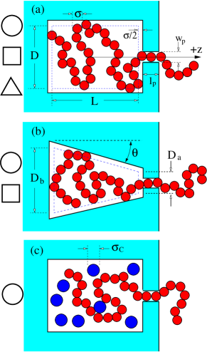
Figure 1: Illustration of the system studied in this work. (a) The polymer translocates through a cylindrical pore of length $l_{\rm p}$ and diameter $w_{\rm p}$ from a cavity of dimensions $L$ and $D$, defined by the subspace accessible to the centers of the monomers. The lateral dimension is defined $D=\sqrt{A}$, where $A$ is the constant cross-sectional area of the subspace. (b) As in (a) except the cavity has a varying cross-sectional area. The lateral dimensions of the subspace at the truncated apex and base of the cavity are $D_{\rm a}$ and $D_{\rm b}$, respectively. (c) As in (a), except crowding agents of size $\sigma_{\rm c}$ partially occupy the cavity space. The shapes on the left side of each picture indicate the cavity cross-section shapes examined in each case.

Note that unlike Ref. Polson, 2015 we do not include forces required to actually drive the polymer into the cavity (such as electric forces in the pore or attraction to the cavity surface). Consequently, the free energy is greater inside the cavity than it is outside. Thus, the polymer is spontaneously driven outward from the cavity for the model systems used here. Inclusion of forces that offset the effect of this free energy gradient to drive translocation inward is straightforward but beyond the scope of this study.

III Methods

Monte Carlo simulations employing the Metropolis algorithm and the self-consistent histogram (SCH) methodFrenkel and Smit (2002) were used to calculate the free-energy functions for the polymer-nanopore model described in Section II. The SCH method provides an efficient means to calculate the equilibrium probability distribution ${\cal P}(m)$, and thus its corresponding free-energy function, $F(m)=-k_{\rm B}T\ln{\cal P}(m)$. Here, $m$ is defined as the number of bonds that have crossed the mid-point of the nanopore. Typically, one bond spans this point for any given configuration, and this bond contributes to $m$ the fraction that lies on the cavity side of the point. Note that $m$ is a continuous variable in the range $m\in[0,N-1]$, and $m$$-$1 is essentially the number of monomers inside the cavity. We have previously used this procedure to measure free-energy functions in other simulation studies of polymer translocationPolson et al. (2013); Polson and McCaffrey (2013); Polson and Dunn (2014) as well in studies of polymer segregation under cylindrical confinementPolson and Montgomery (2014); Polson and Kerry (2018) and polymer folding in long nanochannels.Polson et al. (2017); Polson (2018)

To implement the SCH method, we carry out many independent simulations, each of which employs a unique “window potential” of a chosen functional form. The form of this potential is given by:

$${W_{i}(m)}=\begin{cases}\infty,\hskip 22.76219ptm<m_{i}^{\rm min}\cr 0,\hskip 28.45274ptm_{i}^{\rm min}<m<m_{i}^{\rm max}\cr\infty,\hskip 22.76219ptm>m_{i}^{\rm max}\cr\end{cases}$$ (1)

where $m_{i}^{\rm min}$ and $m_{i}^{\rm max}$ are the limits that define the range of $m$ for the $i$-th window. Within each “window” of $m$, a probability distribution $p_{i}(m)$ is calculated in the simulation. The window potential width, $\Delta m\equiv m_{i}^{\rm max}-m_{i}^{\rm min}$, is chosen to be sufficiently small that the variation in $F$ does not exceed a few $k_{\rm B}T$. Adjacent windows overlap, and the SCH algorithm uses the $p_{i}(m)$ histograms to reconstruct the unbiased distribution, ${\cal P}(m)$. The details of the histogram reconstruction algorithm are given in Refs. Frenkel and Smit, 2002 and Polson et al., 2013.

Polymer configurations were generated carrying out single-monomer moves using a combination of translational displacements and crankshaft rotations. In addition, reptation moves were also employed. The trial moves were accepted with a probability $p_{\rm acc}=\min(1,e^{-\Delta E/k_{\rm B}T})$, where $\Delta E$ is the energy difference between the trial and current states. Prior to data sampling, the system was equilibrated. As an illustration, for a $N=601$ polymer chain, the system was equilibrated for typically $\sim 10^{7}$ MC cycles, following which a production run of $\sim 10^{8}$ MC cycles was carried out. On average, during each MC cycle one reptation move and one single-monomer displacement or crankshaft rotation for each monomer is attempted once.

The windows are chosen to overlap with half of the adjacent window, such that $m^{\rm max}_{i}=m^{\rm min}_{i+2}$. The window width was typically $\Delta m=4\sigma$. Thus, a calculation for $N=601$, where the translocation coordinate spans a range of $m\in[0,600]$, required separate simulations for 299 different window potentials. For each simulation, individual probability histograms were constructed using the binning technique with 20 bins per histogram.

In the results presented below, distance is measured in units of $\sigma$ and energy in units of $k_{\rm B}T$.

IV Results

IV.1 Translocation of fully flexible polymers into isometric cavities

We consider first the scaling properties of the free energy of flexible polymers translocating into isometric cylindrical cavities, i.e. cylindrical cavities with an aspect ratio of $r\equiv L/D=1$. Figure 2 shows the variation of $F$ with translocation coordinate $m$ for various cavity volumes and polymer lengths. The free-energy curves are vertically shifted so that $F=0$ at $m=0$. Note that the limiting case of $V$=$\infty$ corresponds to translocation between two semi-infinite subspaces through an infinitely large flat wall. In this case, $F$ is nearly constant with respect to $m$ with only slight decreases near the limiting values of $m=0$ and $m=N-1$. The shape of this profile is well understood and in the case of infinite polymer length is given by $F(m)=(1-\gamma)\ln[(N-m)m]$, where $\lambda\approx 0.69$ is a critical exponent in 3D.Muthukumar (2011) For cavities of finite volume, the free energy increases monotonically with $m$ (except near $m=N-1$). The rate of this increase of $F$ increases as the volume $V$ of the cavity space decreases. This follows from the fact that increasing confinement reduces the number of accessible conformations of the polymer and thus lowers the entropy. The free-energy functions each have positive curvature over most of their range. This results from the fact that as translocation proceeds, the fraction of the cavity space occupied by monomers increases. The reduction in available cavity space means that the loss in conformational entropy upon transfer of each monomer from outside to the inside of the cavity also increases.

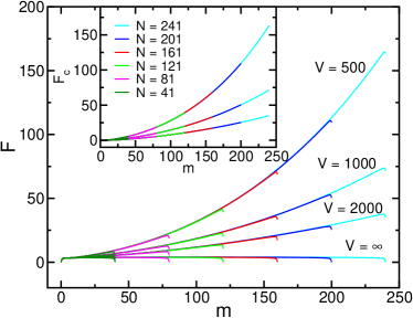
Figure 2: Free energy functions for several polymer lengths ($N$=41, 81, 121, 161, 201 and 241) and a cylindrical cavity of aspect ratio $r=1$. Results for three different cavity volumes are shown. The inset shows $F_{\rm c}$ vs $m$, where $F_{\rm c}(m)\equiv F(m;V)-F_{0}(m)$ and $F_{0}(m)\equiv F(m;V=\infty)$.

Another notable feature in Fig 2 is the overlap of the curves for polymers of different contour lengths entering a cavity of a given volume. This overlap arises from the fact that the confinement free energy of the translocated subchain of length $m$ dominates the total free energy, and the confinement free energy of this portion of the polymer is independent of polymer contour length. We define the confinement free energy as the difference $F_{\rm c}(m)\equiv F(m)-F_{0}(m)$, where $F_{0}(m)\equiv F(m;V=\infty)$ is the free energy for polymer translocation through a flat barrier. To clarify the meaning of $F_{\rm c}(m)$, consider the commonly used approximation that the free energy of a partially translocated polymer is the sum of contributions from two subchains, one of length $m$ on the trans side of the pore, and the other of length $N-m$ on the cis side, each of which is effectively tethered to the pore-containing wall.Muthukumar (2011) Thus, $F(m)=F^{\rm(cw)}_{\rm trans}(m)+F^{\rm(cw)}_{\rm cis}(N-m)$ and $F_{0}(m)=F^{\rm(w)}_{\rm trans}(m)+F^{\rm(w)}_{\rm cis}(N-m)$, where “w” denotes tethering to a wall and “c” denotes the presence of cavity confinement. For the systems considered in this work illustrated in Fig. 1 the confinement only affects the trans subchain. It follows that $F^{\rm(cw)}_{\rm cis}(N-m)=F^{\rm(w)}_{\rm cis}(N-m)$, and so $F_{\rm c}(m)=F^{\rm(cw)}_{\rm trans}(m)-F^{\rm(w)}_{\rm trans}(m)$. Thus, $F_{\rm c}(m)$ can be interpreted as the additional free energy of a polymer tethered to a hard wall arising from a reduction in the conformational entropy due to the cavity confinement. The approximation employed neglects subtle effects from the pore that lead to oscillations in the free energy, as described in detail in Ref. Polson et al., 2013. However, it can be shown that subtraction of $F_{0}(m)$ from the free-energy function eliminates this feature in $F_{\rm c}(m)$. The confinement free-energy functions for the data of Fig. 2 are shown in the inset of the figure. Note that the small deviations from perfect overlap for $F(m)$ are now gone and the $F_{\rm c}(m)$ overlap perfectly for all $N$ at each cavity volume, as expected. (The deviations from perfect overlap for the $F(m)$ curves are due to the non-extensive part of the free energy of a wall-tethered polymer, which also gives rise to the slight curvature in the free-energy curves in the absence of confinement ($V$=$\infty$).)

Let us now examine the scaling properties of $F_{\rm c}(m)$. Figure 3 shows the confinement free energy for polymers with lengths ranging from $N$=101 to 601. For convenience, each simulation was carried out for a cavity volume chosen so that the packing fraction in the cavity at $m=N-1$ was $\phi=0.15$; consequently, the cavity volume was proportional to the polymer length. The variation of $F_{\rm c}$ with $m$ can be estimated using scaling arguments developed for polymer solutions in the semi-dilute regime. Here, the confined section of the polymer can be viewed as a collection of blobs, each with a size of $\xi\sim\phi^{\nu/(1-3\nu)}$, where $\phi\sim m/V$ is the packing fraction and $\nu\approx 0.588$ is the Flory exponent.Rubinstein and Colby (2003) Since the number of blobs is $n_{\rm b}\approx V/\xi^{3}$ and each blob contributes of order $kT$ to the confinement free energy, it follows that

$$F_{\rm c}/kT\sim V^{-\alpha}(m-1)^{\beta},$$ (2)

where $\alpha$=1.31 and $\beta$=2.31. Note that we have substituted $m\rightarrow m-1$ to account for the finite length of the pore, which holds approximately one monomer. Also note that the commonly employed approximation of $\nu=\frac{3}{5}$ leads to a slightly different scaling of $F_{\rm c}/kT\sim V^{-1.25}(m-1)^{2.25}$. Previous work has shown that the semi-dilute regime scaling is accurate for packing fractions of $\phi<0.15$,Cacciuto and Luijten (2006b), which is the motivation here for choosing the cavity volume to be such that $\phi$=0.15 at full insertion. As a consequence, the condition that $\phi<0.15$ is satisfied for all $m$. A lower limit on the range of validity for this prediction is the requirement that the number of blobs $n_{\rm b}\approx(m-1)\phi^{1/(3\nu-1)}$ satisfy $n_{\rm b}\gg 1$. For the polymer lengths considered here, it is not possible to find a range of $m$ that satisfies both conditions simultaneously. To analyze the data, we follow the approach taken in our previous studyPolson (2015) and use the more relaxed condition for low density of $n_{\rm b}\geq 3$.

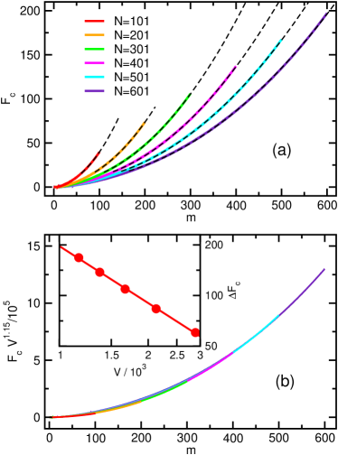
Figure 3: (a) Free energy difference $F_{\rm c}=$ vs $m$ for polymers of different lengths. In each case, the confinement cavity is a cylinder with an aspect ratio of $D/L$=1 and a volume determined by the condition that the packing fraction for $m=N-1$ is $\phi_{\rm c}=0.15$. The dashed lines show fits to the curves for a fitting function of the form $F_{\rm c}=c_{0}+c_{1}(m-1)^{\beta}$. The minimum $m$ of the fitting curves is the minimum of the range over which the $F_{\rm c}$ was fit. The fitting exponents are $\beta$=2.01, 2.05, 2.08, 2.10, 2.11 and 2.13 for $N$=101, 201, 301, 401, 501 and 601, respectively. (b) Scaled free-energy functions using the data from (a), where the scaling $F_{\rm c}V^{1.15}$ leads to data collapse, as explained in the text. The inset shows the variation of $\Delta F_{\rm c}(\equiv F_{\rm c}(m=N))$ vs cavity volume for a $N$=401 polymer entering a cavity with $D/L=1$. The solid line shows a fit to a power law $\Delta F_{\rm c}\sim V^{\alpha}$, where the fit yielded a scaling exponent of $\alpha$=$1.12\pm 0.02$.

Figure 3(a) shows the results of fits to each of the confinement free-energy functions using a fitting function of the form $F_{\rm c}=c_{0}+c_{1}(m-1)^{\beta}$, where $c_{0}$, $c_{1}$ and $\alpha$ are fitting coefficients. The best fit curves are plotted on the graph as dashed lines. The lower bounds of the plotted fitting curves mark the lower limit of the range of the simulation data that were included in the fit, i.e. the point where $n_{\rm b}=3$. The fitting exponents were measured to be $\beta$=2.01, 2.05, 2.08, 2.10, 2.11 and 2.13 for $N$=101, 201, 301, 401, 501 and 601, respectively. These values are underestimates of the predicted scaling exponent of $\beta=2.31$. This is clearly a finite-size effect, as suggested by the fact that $\beta$ tends (slowly) toward the predicted value as the system size increases. As noted above, a different cavity volume was used for each simulation. Equation (2) predicts that the scaling $F_{\rm c}V^{1.31}$ should collapse these functions onto a universal curve if we scale using the volume $V$ employed in each of the simulations. As is evident in Fig. 3(b), we find scaling with somewhat smaller exponent, i.e. $F_{\rm c}V^{1.15}$, produces the best collapse. As with the small discrepancy in the observed and predicted variation of $F_{\rm c}$ with respect to $m$, this difference is undoubtedly due to finite-size effects. To further investigate the volume dependence of $F_{\rm c}$, we examine the case of translocation of a $N$=401 polymer into a $r$=1 cavity of different volumes. We define the confinement free energy at full insertion to $\Delta F_{\rm c}\equiv F_{\rm c}(m$=$N$$-$$1)$. The inset of Fig. 3(b) shows the variation of $\Delta F_{\rm c}$ with $V$ in cases where the cavity volume fraction at full insertion was $\phi_{\rm c}$=0.06, 0.08, 0.1, 0.12 and 0.14. Fits to a power law yield a scaling of $\Delta F_{\rm c}\sim V^{-1.12\pm 0.02}$. Again we find a discrepancy between the measured exponent and that predicted using scaling arguments.

The discrepancies between the measured and predicted scaling exponents $\alpha$ and $\beta$ are somewhat smaller than those obtained in our previous study of translocation into spherical cavities (a special case of ellipsoidal cavities that were studied).Polson (2015) This is likely due to the shorter polymer lengths considered in that study ($N\leq 140$) and further supports our claim that they are due to finite-size effects.

It is worth noting here that the confinement free energy calculated in the simulations is that for a polymer whose end monomer is effectively tethered to a point on the inner surface of the confining cavity. This is due to the fact that when $m$=$N$-$1$, a single monomer is still located in the nanopore. On the other hand, the theoretical model imposes no such condition. In principle, the difference in confinement free energies for these two cases will contribute to the discrepancy. In a recent study, we described a method to calculate the free-energy cost of localizing an end monomer of a confined polymer.Polson and McLure (2019) Using the same model for flexible chains as that employed here we find that for polymer lengths and packing fractions comparable to those used here that the end-monomer localization free energy was 1–2 $k_{\rm B}T$. Thus, the effect is very small and unlikely to be the principal cause of the discrepancy.

Why do finite-size effects lead to effective scaling exponents that are lower than the predicted values? Some insight is provided by the arguments presented by Sakaue in Ref. Sakaue, 2007. The scaling prediction derived above begins with the assumption that $F_{\rm c}\sim n_{\rm blob}=V/\xi^{3}$, which implicitly assumes that the monomer density is uniform throughout the enclosed space. However, Sakaue notes that monomer depletion in a layer of width $\approx\xi$ near the surface of the cavity is expected. This gives rise to a surface correction term to the free energy, $\Delta F_{\rm surf}$, which is approximated as a surface integral $\Delta F_{\rm surf}=\int da(\Pi\times\xi)$, where the osmotic pressure is given by $\Pi\approx k_{\rm B}T/\xi^{3}$. This is approximately $\Delta F_{\rm surf}=\Pi\xi A_{\rm s}$, where $A_{\rm s}\sim D^{2}$ is the surface area of the cavity. Noting again that $\xi\sim\phi^{1/(1-3\nu)}$, it follows that

$$\Delta F_{\rm surf}/k_{\rm B}T\sim D^{-0.87}(m-1)^{1.54}.$$ (3)

(Using $\nu=\frac{3}{5}$ gives $\Delta F_{\rm surf}/k_{\rm B}T\sim D^{-0.83}(m-1)^{1.5}$.) Comparing Eqs. (2) and (3), we see that the exponents for $D$ and $m-1$ in the case of the surface term $\Delta F_{\rm surf}$ are each smaller than those for the volume term (i.e. $0.87<1.31$ and $1.54<2.31$). For a sufficiently small cavity, the surface term could be an appreciable contribution to the total free energy. For the results shown in Fig. 3, this appears to be the case, and the smaller scaling exponents of the surface term reduce the values of the measured effective exponents. A thorough investigation of this effect requires additional calculations with much larger cavity sizes where the volume of the depletion layer near the surface is a much smaller fraction of the entire cavity volume. However, this also necessitates using polymers at least an order of magnitude longer, which is currently not feasible.

IV.2 Effects of confinement shape

We now consider how the free energy is affected by varying the both the geometry type and the shape anisometry of the cavity. In this section we examine translocation into cavities with constant cross-sectional area for the cases of cylindrical, rectangular and triangular cross-sections as illustrated in Fig. 1(a). Figure 4(a) shows the confinement free energy $\Delta F_{\rm c}$ vs cavity length $L$ for three different cavity types, each with three different values of cavity width $D$. Results are shown for a polymer of length $N$=201. Several trends are notable. First, for all cavity dimensions $D$ and $L$ the confinement free energy is greatest for triangular cavities and lowest for cylindrical cavities. This is due to the effect of entropic depletion, in which the monomer density is significantly reduced in sharp corners of confined spaces.Manneschi et al. (2013); Reinhart et al. (2013); Polson (2018) This effect tends to be especially strong in triangular cavities, which have the sharpest angles, and is absent for the case of cylindrical confinement. Such monomer depletion in these regions leads to an effective cross-sectional area that is less than the actual area accessible to the monomer centers. Since decreasing the area and therefore $D$ increases the confinement and therefore the free energy, the trends with regard to cross-section shape follow accordingly.

Another trend is that for sufficiently long channels $\Delta F_{\rm c}$ is invariant with respect to $L$. This results simply from the fact that a polymer in a sufficiently long tube is insensitive to the presence of longitudinal confinement. Thus, decreasing $L$ in this range does not reduce the number of accessible conformations and decrease the entropy. However, as $L$ is further reduced the polymer is uniformly compressed along the channel, leading to entropy loss and the observed increase in $\Delta F_{\rm c}$. The onset of the effects of longitudinal confinement upon decreasing $L$ occurs at higher values of $L$ for narrower channels, reflecting the fact that the extension length is greater for smaller channels widths. In addition, $\Delta F_{\rm c}$ decreases with increasing channel width at each fixed tube length. This is a consequence of the fact that narrower channels distort the polymer more relative to the unconfined state, leading to a greater reduction in entropy.

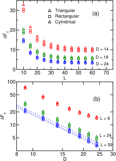
Figure 4: (a) Confinement free energy $\Delta F_{\rm c}$ vs cavity length for various cavity geometries. Results are shown for a polymer of length $N$=201 for three different cavity widths. (b) Confinement free energy $\Delta F_{\rm c}$ vs cavity width $D$ for various cavity geometries. Results are shown for a polymer of length $N$=201 for cavity lengths of $L$=9 (red symbols), $L$=24 (green symbols) and $L$=59 (blue symbols). The blue dashed lines for $L$=59 are fits to a power law, $\Delta F_{\rm c}\sim D^{-\beta}$, which yield exponents of $\beta=1.82\pm 0.03$ (triangular), $\beta=1.87\pm 0.03$ (rectangular), and $\beta=1.87\pm 0.03$ (cylindrical).

Figure 4(b) shows the variation of $\Delta F_{\rm c}$ with $D$ for the same three cavity geometries and for three different cavity lengths. Consistent with the results of Fig. 4(a), $\Delta F_{\rm c}$ increases with decreasing cavity length at any given $D$. In addition, the trend with regard to channel shape (i.e. $\Delta F_{\rm c}$ for triangular channels is greater than those for square channels, which in turn is greater than those for cylindrical channels) still holds. In the case of $L$=59, where the effects of longitudinal confinement are negligible for this polymer length ($N$=201), the polymer behaves simply as one confined to an infinitely long channel. For this confinement, the de Gennes blob model predicts a confinement free energy that scales as $\Delta F\sim D^{-1/\nu}\approx D^{-1.70}$ (for $\nu\approx 0.588$). We have fit the $L$=59 data to a power law $\Delta F\sim D^{-\beta}$, and the fitting curves overlaid on the data in Fig. 4(b) show that the data does indeed exhibit power-law behaviour. However, the measured scaling exponents of $\beta=1.82\pm 0.03$ for triangular channels, $\beta=1.87\pm 0.03$ for rectangular channels, and $\beta=1.87\pm 0.03$ for cylindrical channels deviate somewhat from the predicted value. It is unlikely that this discrepancy arises from confinement cavities that are insufficiently wide since the condition that $D\gtrsim 10$ for blob-model scaling behaviour to emerge noted in a previous studyKim et al. (2013) is satisfied here. Instead, it arises from the fact that the chains are insufficiently long, leading to a violation of the condition that the number of blobs satisfies $n_{\rm b}\gg 1$, which is also necessary to recover the predicted scaling.

Figure 5(a) shows the variation of $\Delta F_{\rm c}$ with the cavity aspect ratio $r\equiv L/D$ at fixed volume for three different cavity shapes. Data are shown for a volume of $V$=1000, which corresponds to $V/R_{\rm g}^{3}=0.64$, where $R_{\rm g}=11.60$ is the radius of gyration for an unconfined $N$=201 polymer. At all aspect ratios, the same patterns noted in Fig. 4 are observed, i.e, the confinement free energy is greatest for triangular cavities and lowest for cylindrical cavities. Notably, for all three geometries, $\Delta F_{\rm c}$ is a minimum at an aspect ratio of $r$=1, i.e. for equal lateral and longitudinal cavity dimensions. The same trend is observed for other cavity volumes (data not shown). The curves are approximately symmetric about $r$=1 on a logarithmic scale. This indicates that the confinement free energy for aspect ratios of $r$ and $1/r$ appear to be roughly equal, though some degree of asymmetry is evident. This asymmetry is more visible in Fig. 5(b), which shows the relative difference in the confinement free energy $\zeta_{\rm r}\equiv(\Delta F_{\rm c}(r)$$-$$\Delta F(r$=$1))/\Delta F_{\rm c}(r$=$1)$ as a function of cavity volume for the cases of $r$=1/4 and $r$=4. For all cavity geometries $\zeta_{4}>\zeta_{1/4}$. This is an illustration of the general trend that “prolate” cavities ($L>D$) have a higher confinement free energy than “oblate” cavities ($L<D$). This trend is consistent with results of our previous study that examined translocation into ellipsoidal cavitiesPolson (2015) and demonstrates that it is a generic effect independent of the details of the cavity shape. The inset shows the absolute difference, $\Delta F_{\rm c}^{\dagger}(r)$$\equiv$$\Delta F_{\rm c}(r)$$-$$\Delta F(r$=$1)$ for $r=4$ and $r=0.25$ and is a measure of the degree of asymmetry of the free energy for “prolate” and “oblate” cavities of the same volume. Interestingly, $\Delta F_{\rm c}^{\dagger}$ exhibits a maximum near $V/R_{\rm g}^{3}\approx 0.5$.

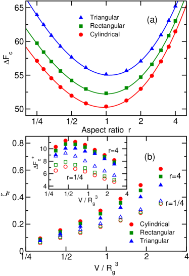
Figure 5: (a) Confinement free energy $\Delta F_{\rm c}$ vs cavity shape anisometry, $r$. Results are shown for polymer of length $N$=201 and for cavities of various geometry, each with a volume of $V$=1000 (i.e. $V/R_{\rm g}^{3}$=0.67). (b) Relative difference in the confinement free energy $\zeta_{\rm r}$ vs scaled cavity volume $V/R_{\rm g}^{3}$, where $\zeta_{\rm r}\equiv(\Delta F_{\rm c}(r)$$-$$\Delta F(r$=$1))/\Delta F_{\rm c}(r$=$1)$ and where $R_{\rm g}$ is the radius of gyration of a free polymer. Data are shown for anisometry ratios of $r$=4 and $r$=0.25 for triangular, rectangular and cylindrical cavities and for polymers of length $N$=201. The solid symbols correspond to $\zeta_{4}$ and the open symbols are for $\zeta_{0.25}$. The inset shows the absolute difference in confinement free energy, $\Delta F_{\rm c}^{\dagger}(r)$$\equiv$$\Delta F_{\rm c}(r)$$-$$\Delta F(r$=$1)$ vs $V/R_{\rm g}^{3}$ using the same data.

A naive application of the approximation borrowed from the theory of semidilute polymer solutions that the free energy is proportional to the number of blobs, i.e. $F_{\rm c}/k_{\rm B}T=V/\xi^{3}$ where the correlation length scales as $\xi=\phi^{-0.77}$, suggests that $F_{\rm c}$ should depend only on the cavity volume and not its shape. The observed dependence of the confinement free energy on the cavity shape is most likely a result of the breakdown of this approximation in the limit of small cavities where $\xi$ is of the order of one or more cavity dimensions. In the case of $V$=1000 and $N-1$=200 for the data in Fig. 5, full insertion of the polymer leads to a volume fraction of $\phi_{\rm c}=0.1047$, and thus a correlation length of approximately $\xi=\phi^{-0.77}\approx 5.7$. In the case of cylindrical cavities where $r$$\equiv$$L/D$=$1$, $D$=$L$=10.9. However, for $r$=4, $D$=6.8 and $L$=27.3, while for $r=1/4$, $D$=17.2 and $L$=4.3. In these latter cases, the smallest dimension $l_{\rm min}\equiv{\rm min}(L,D)$ is very close to the estimated blob size. Evidently, in the regime where $l_{\rm min}={\cal O}(\xi)$, an increase in the ratio $\xi/l_{\rm min}$ leads to an increase in the free energy. As the volume decreases and the volume fraction increases, the blob size decreases. Thus, the effect is expected to be less significant, consistent with the observed decrease in $\xi_{\rm r}$ with decreasing $V$ in Fig. 5.

IV.3 Translocation into tapered confinement spaces

Let us now consider the case of translocation into spaces with tapered geometries, illustrated in Fig. 1(b). We consider first the case of a cavity shaped as a truncated pyramid. As noted earlier, this choice is relevant to previous experimental studies that have employed a pore-cavity-pore device to study DNA translocation into and out of pyramidal cavities.Pedone et al. (2011); Langecker et al. (2011) Here we examine the effects of size, shape and nanopore location (i.e. at the apex or the base) on the translocation free energy. In our calculations, we fix truncation section width to $D_{\rm a}=2$.

Figure 6 shows the variation in confinement free energy $\Delta F_{\rm c}$ with the taper angle $\theta$, which is illustrated in Fig. 1(b). Results are shown for a polymer of length $N$=201 entering the cavity from either the base or the apex of the pyramid. We also consider two different cavity volumes. For all values of the taper angle, the confinement free energy increases with decreasing volume, as expected. In each case there is a broad minimum of $\Delta F_{\rm c}$ with respect to $\theta$. This qualitatively similar to the trend observed in Fig. 5(a) for the aspect ratio in the case of constant cross-sectional area geometries. This is not surprising, as the value of the taper angle $\theta$ determines the base/height ratio of the pyramid, which is the equivalent of the aspect ratio for this type of geometry. As a reference, the base/height ratio is unity when $\theta=\tan^{-1}(0.5)=26.6^{\circ}$. The location of the minimum is $\theta_{\rm min}\approx 20^{\circ}$ for all cases except for the case of $V/R_{\rm g}^{3}=3$ and translocation through the apex.

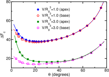
Figure 6: Confinement free energy $\Delta F_{\rm c}$ vs taper angle $\theta$ for polymer translocation into a truncated pyramid. The taper angle of the pyramid is labeled in Fig. 1(b). Results are shown for a $N$=201 polymer for various cavity volumes, each for translocation through a pore in the pyramid base and through a pore at the pyramid apex. The solid lines are guides for the eye.

A more notable feature is the contrast between apex- and base-entry translocation. At high density, $\Delta F_{\rm c}$ for the two cases converge at large $\theta$ (i.e “squat” pyramids). However, as $\theta$ decreases and the pyramids become “taller”, $\Delta F_{\rm c}$ for apex-entry translocation becomes increasingly greater than that for base-entry. This trend is connected to the phenomenon of entropic depletion in the corners of the pyramid. Recall that this depletion effect was also the cause of the difference in the values of $\Delta F_{\rm c}$ for cavities of different cross-section shapes shown in Figs. 4 and 5. We propose the following explanation for the observed trends. As $\theta$ decreases, the apex becomes sharper and the polymer that enters through the base avoids occupying the region near the apex. However, apex-entry translocation necessarily constrains a portion of the polymer to remain in the apex region in opposition to the tendency for depletion. The strong confinement of that part of the polymer ultimately leads to a reduction in conformational entropy and thus a higher free energy relative to the case of base-entry translocation where depletion in the apex does occur. Depletion for the base-entry case increases as the apex narrows, and thus the difference between the free energies grows with decreasing $\theta$. For large $\theta$ (i.e. a wide apex), the entropic depletion for base-entry is negligible, and thus $\Delta F_{\rm c}$ for the two cases converge in this limit. As $V$ decreases (i.e. as the density increases) the monomers are likely pushed deeper into all the corners of the pyramid. Thus, entropic depletion near the apex in the case of base-entry translocation is reduced and the difference between $\Delta F_{\rm c}$ for the two cases lessens even for small $\theta$, as is evident by a comparison of the results for the two volumes in Fig. 6. A rigorous test of this explanation would benefit from future measurement of the density distribution in the cavity upon variation in its size and shape.

Now we consider the case of translocation into a very narrow and gradually tapered space. We choose $L$=$\infty$ and a circular cavity cross section, i.e. an infinitely long cone. The free energy and dynamics of polymers in such conical spaces have been the subject of other theoretical and simulation studies, Su and Purohit (2011); Nikoofard et al. (2013); Nikoofard and Fazli (2015); Kumar and Kumar (2018) and the behaviour of DNA in conical channels has been examined in experimental studies.Peters (2010) Figure 7 shows the confinement free energy $\Delta F_{\rm c}$ of a flexible polymer translocating into an infinitely long cone. The free energy is calculated as the difference $F_{\rm c}(m)\equiv F_{\rm cone}(m)-F_{\rm 0}(m)$ between the free-energy function for the translocation into the cone, $F_{\rm cone}(m)$, and that for the planar geometry, $F_{0}(m)$. The nanopore is located on a truncation surface cross-section of diameter $D_{0}=6$.

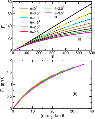
Figure 7: (a) Confinement free energy $F_{\rm c}$ vs degree of translocation $m$ for translocation into an infinitely long truncated cone. Results are shown for $N=601$ for different values of the cone angle $\theta$. The diameter of the truncation cross section containing the pore is $D_{0}$=9. Overlaid on the solid curves for simulation data are fits using Eq. (LABEL:eq:Fcone2). (b) The same data as in (a) plotted on scaled and shifted axes. The translocation coordinate shift value is $m_{0}=8$, as explained in the text.

To analyze the results, we follow the approach taken in Ref. Nikoofard and Fazli, 2015 and derive an expression for $F_{\rm c}(m)$ using the de Gennes blob model. First note that the diameter of the cone is given by $D(z)=D_{0}+2z\tan\theta$, where $\theta$ is the taper angle, illustrated in Fig. 1, and $z$ is the distance from the pore along the central axis of the cone. The blob size of the portion of the polymer confined in the cone is $\xi(z)\approx D(z)$, and the number of monomers in each blob is $g(z)\sim(\xi(z))^{1/\nu}$. The number of monomers $dn$ in a slice of thickness $dz$ is $dn(z)\sim(g(z)/\xi(z))dz$, and so the linear density of monomers along the cone, $\lambda(z)\equiv dn/dz$ scales as $\lambda(z)\sim(\xi(z))^{1/\nu-1}$. If the extension of the $m$ monomers of the polymer in the cone along $z$ is $R_{||}$, it follows that $m\sim\int_{0}^{R_{||}}\lambda(z)dz$. Thus,

$$m=\frac{B}{\tan\theta}\left[(D_{0}+2R_{||}\tan\theta)^{1/\nu}-D_{0}^{1/\nu}\right],$$ (4)

where $B$ is a proportionality factor of order unity. In addition, the free energy due to the tube confinement can be determined by noting that each blob contributes of the order of $kT$ to the confinement free energy. In the case of a continuously varying blob length, this implies that $F_{\rm c}/kT\sim\int_{0}^{R_{||}}[\xi(z)]^{-1}dz$. It follows that

$$\frac{F_{\rm c}}{kT}=\frac{A}{\tan\theta}\left[\ln(D_{0}+2R_{||})\tan\theta)-\ln D_{0}\right],$$ (5)

where $A$ is another proportionality factor of order unity. Solving Eq. (4) for $R_{||}$ and substituting this expression into Eq. (5), we find that

$$\frac{F_{\rm c}(m)}{kT} = \left(\frac{A}{\tan\theta}\right)\ln\left[\frac{2}{D_{0}}\left(\frac{(m-m_{0})}{B}\tan\theta+D_{0}^{1/\nu}\right)^{\nu}-1\right]$$

Note in the final step we have made the substitution $m\rightarrow m-m_{0}$. This shift in the translocation is required to correct for the fact that $F_{\rm c}$ is otherwise predicted to increase monotonically for $m\geq 0$. In practice, this is not the case, as several monomers must first enter the cone from the pore before the effects of lateral confinement are felt. This value is expected to increase with $D_{0}$. For $D_{0}=9$, we find that $F_{\rm c}$ is zero until $m$ has a threshold value of $m_{0}=8$. Equation (LABEL:eq:Fcone2) predicts that the free energies for all cone angles should fall on a universal curve when plotting $F_{\rm c}\tan\theta$ vs $(m-m_{0})\tan\theta$. Figure 7(b) shows that the data come close to collapse on such a universal curve, though small discrepancies remain. Overlaid on the calculated curves in Fig. 7(a) are fits using Eq. (LABEL:eq:Fcone2). Generally, the quality of each fit is excellent. However, we note that the fitting parameter values for the fits for each angle vary in the range $A=1.90-2.14$ and $B=0.487-0.502$. This small variation is consistent with the good but imperfect data collapse for the scaled data in the Fig. 7(b).

IV.4 Effects of polymer stiffness

We now examine the effects of polymer stiffness on the translocation free energy. Given the rich scaling behaviour expected for the confinement free energy of semiflexible polymers upon variation in the persistence and contour lengths as well as the cavity dimensions,Sakaue (2018) we choose to focus on two important limiting cases and defer a more complete exploration of parameter space to a future study. In particular, we choose to examine translocation cavities with: (1) an aspect ratio of $r\equiv L/D=1$, and (2) and aspect ratio of $r\gg 1$.

Figure 8(a) shows the confinement free-energy function $F_{\rm c}(m)$ for a $r$=1 cavity in the case of a $N$=201 polymer of persistence length $P$=5. Results for various cavity sizes are shown. The key trend is an increase in the confinement free energy as $D$ decreases. There are two contributions to this effect. First, as in the case of flexible polymers, a reduction in the cavity size will reduce the number of available conformations of the polymer, thus reducing the entropy. Second, as cavity size is decreased the polymer is increasingly forced to bend, leading to an increase in the mean bending energy and thus the free energy. The inset of Fig. 8(a) shows the variation of $\Delta F_{\rm c}$ with $D$ for semiflexible polymers of stiffness $\kappa$=5 and 10, as well as for a fully flexible polymer ($\kappa$=0). In the range of $D=9-35$, the data appear to scale as $\Delta F_{\rm c}\sim D^{-\gamma}$, though there is a slight deviation from power-law scaling for small cavities with $D\lesssim 12$. Fits in the domain $D\geq 13$ yield exponents of $\gamma=2.04\pm 0.02$ for $\kappa$=10, $\gamma=2.30\pm 0.03$ for $\kappa$=5, and $\gamma=2.76\pm 0.03$ for a fully flexible polymer. Figure 8(b) shows the variation of $\Delta F_{\rm c}$ with $P$ in the domain $P=4-15$ for cavities of various size. Again, the scaling of data appears to follow a power law of the form $\Delta F_{\rm c}\sim P^{\beta}$, where fits to the data yield scaling exponents of $\beta$=0.54, 0.66, 0.72 and 0.75 for $D$=19, 27, 31 and 35, respectively.

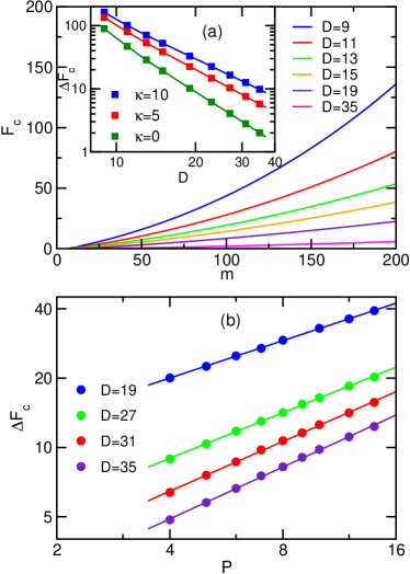
Figure 8: (a) Confinement free energy, $F_{\rm c}$ vs $m$ for a semiflexible polymer of contour length $N$=201 and stiffness $\kappa$=5 (i.e. persistence length $P$=5) translocating into a cylindrical cavity with an aspect ratio of $D/L$=1. Results are shown for various values of cavity sizes. The inset shows the $\Delta F_{\rm c}$ vs $D$ for polymers of stiffness $\kappa$=10, 5 and 0 (i.e. full flexible). Fits to $\Delta F_{\rm c}\sim D^{-\gamma}$ in the region $D\geq 14$ yields exponents $\gamma$=2.08, 2.35 and 2.80 for $\kappa$=10, 5 and 0, respectively. (b) $\Delta F_{\rm c}$ vs persistence length $P$ for $N$=201 and $D/L$=1. Results are shown for four different cavity sizes. The solid lines are fits to $\Delta F_{\rm c}\sim P^{\beta}$, where $\beta$=0.54, 0.66, 0.72 and 0.75 for $D$=20, 28, 32 and 36, respectively.

If the system was in a well-defined scaling regime such that the confinement free energy satisfied $\Delta F_{\rm c}\sim D^{-\gamma}P^{\beta}$, the value of $\gamma$ would not depend on $P$, nor would the value of $\beta$ change with $P$. As noted above, however, such dependencies are observed. One possibility is that the fits have merely yielded effective exponents in a cross-over region between well-defined scaling regimes. To clarify this issue let us consider the theoretical studies of Sakaue,Sakaue (2007, 2018) who has predicted a number of free energy scaling regimes for semiflexible polymers in closed spaces upon variation in the polymer contour and persistence lengths and the cavity dimensions. The boundaries between the regimes depend on the polymer length, $N=L_{\rm c}/\sigma$, cavity size $D$, and the ratio $p\equiv l_{\rm K}/\sigma=2P/\sigma$, where $l_{\rm K}$ is the Kuhn length. (We use the notation of the present article and the convention for the definition of $N$ in Ref. Sakaue, 2007 rather than Ref. Sakaue, 2018.) In our calculations, $N\ll p^{3}$ in all cases and thus the scaling of the fluctuating semidilute regime (regime I from Ref. Sakaue, 2007 and $\rm F^{3}_{~{}0}$ in Ref. Sakaue, 2018) is not expected to relevant to our results. (It does, however, provide the correct scaling with respect to $D$ for flexible polymers.) On the other hand, we note that $N\approx p^{2}$ and $D\gtrsim p$. As a consequence, the system is expected to be in a region of parameter space near the convergence of the following four scaling regimes illustrated in Fig. 2 of Ref. Sakaue, 2007: (a) the mean-field semidilute regime (regime II), where $\Delta F_{\rm c}/k_{\rm B}T\sim N^{2}D^{-3}P^{0}$; (b) the liquid crystalline regime (regime III), where $\Delta F_{\rm c}/k_{\rm B}T\sim N^{1}D^{0}P^{-1}$; (c) the ideal chain regime (regime IV), where $\Delta F_{\rm c}/k_{\rm B}T\sim N^{1}D^{-2}P^{1}$; (d) the bending regime (regime V), where $\Delta F_{\rm c}/k_{\rm B}T\sim N^{1}D^{-2}P^{1}$. (Note that in Ref. Sakaue, 2018 these regimes are labeled $\rm M^{3}_{~{}0}$, $\rm N^{3}_{~{}0}$, $\rm I_{0}$, and $\rm S_{0}$, respectively.) The effective scaling exponents extracted from fits to our data are qualitatively inconsistent with regime III and so suggest the system is in a transition region between regime II and regimes IV/V (note that the latter two satisfy the same scaling). In particular, the measured $\gamma$ lies between the values for those regimes of $\gamma=2$ and $\gamma=3$. Likewise, the measured value of $\beta$ lies between the values for those regimes of $\beta=0$ and $\beta=1$. Note as well that increasing $D$ leads to a measured scaling exponent $\beta$ closer to the value of $\beta=1$ predicted for regime IV, consistent with the trends of the scaling regime boundaries in Fig. 2 of Ref. Sakaue, 2007. Likewise, increasing $\kappa$, and therefore $P$, leads to an exponent $\gamma$ that tends toward the value of $\gamma=2$ for regime IV, which is also qualitatively consistent with the trends for the confinement regimes predicted in Ref. Sakaue, 2007.

One feature of the present system that complicates a comparison of our results with Sakaue’s predictions is the fact that here $\Delta F_{\rm c}$ represents the confinement free energy of a polymer that is effectively tethered to one wall of the cavity (because one monomer still lies in the pore when $m=N-1$). As noted in Ref. Polson and McLure, 2019 for the case of flexible chains the free-energy cost of such tethering is only 1–2 $k_{\rm B}T$ for polymers of comparable length and packing fraction as that considered here. Thus, the effect on on the free energy is expected to be negligible. However, for stiff chains this tethering also leads to an orientational anchoring to the cavity wall with the chain contour tending to be perpendicular to the wall at the effective tethering point (i.e. the pore). It is possible that this feature will alter the confinement free energy in a manner that could further perturb the scaling properties of the free energy.

Obviously, this analysis of our simulation results represents nothing like a rigorous test of the predictions of Refs. Sakaue, 2007 and Sakaue, 2018. At a minimum, such a test requires using polymers of substantially greater length in order for a system to lie unambiguously in a well-defined scaling regime rather than in a transition region. Nevertheless, our results do at least provide some tentative and indirect supporting evidence for the scaling predictions.

Having first considered the case of translocation of semiflexible polymers into cavities with aspect ratios of $r$=1, let us now consider the case of highly asymmetric cavities with $r\gg 1$. In addition, we also focus on very narrow cavities such that $D\lesssim P$. In the case of very long cavities where $L>L_{\rm c}$ (where $L_{\rm c}$ is the polymer contour length), this corresponds to the Odijk or backfolded Odijk regimes. However, for $L<L_{\rm c}$ the finite cavity length is expected to produce different conformational behaviour. Figure 9 (a) shows free-energy functions for a semiflexible polymer of length $N$=201 entering a cylindrical cavity of width $D$=4. Results are shown for polymers of varying degrees of rigidity ranging from fully flexible to $\kappa$=15. In each case, curves are shown for a cavity of length $L$=50 (solid curves) and $L$=$\infty$ (dashed curves). Functions for different $\kappa$ are vertically shifted relative to each other for clarity. The curves for each $\kappa$ initially overlap at low $m$, where the translocated part of the polymer is not sufficiently long to feel the effects of longitudinal confinement for $L$=50. As $m$ increases further, the free-energy functions for the longitudinally confined systems diverge from the $L$=$\infty$ curves at the point where the polymer makes contact with the confining cap. The free energy increase with respect to the $L$=$\infty$ case arises from the reduction in the conformational entropy resulting from this additional confinement. As expected, the value of $m$ at which the divergence occurs decreases with increasing polymer stiffness. This follows from the fact that stiffer polymers are more elongated in the tube, and thus fewer translocated monomers are required before the polymer reaches the cap. For $P<D$, $F$ increases smoothly with positive curvature. However, for $P\gtrsim D$, curves are qualitatively different in that $F$ increases markedly in steps with linear regimes in between. The size of the step increases with $\kappa$ and the locations of the steps appear to converge to values of $m$ that are integer multiples of approximately $\Delta m$=55.

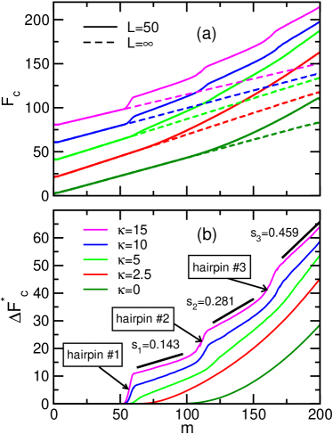
Figure 9: (a) Free energy for translocation of a semiflexible polymer of length $N$=201 into a cylindrical channel of width $D=4$. Results are shown for various degrees of polymer stiffness for cylinders of length $L$=25 and $L$=$\infty$. The curves are vertically shifted and spread out along the vertical axis to minimize overlap for clarity. (b) Difference in the free energy, $\Delta F_{\rm c}^{*}\equiv F_{\rm c}(m;L=50)-F_{\rm c}(m;L=\infty)$ vs $m$. The black line segments in the inset are linear fits (shifted upward) to the linear sections of the $\kappa=15$ curve. The slopes of the fits are each labeled, as are the locations of each hairpin that separate the linear regions.

The origin of the step behaviour is straightforward. In the case of the more flexible chains, increasing $m$ will typically cause a gradual increase in the density of monomers, which will likely maintain their linear organization along the channel, i.e. a longitudinally uniform compression. At high density (i.e. high $m$), the translocated portion of the polymer may lose its linear organization as it forms backfolds, but no obvious signature in $F_{\rm c}(m)$ is expected. By contrast, a stiffer polymer is expected to initially undergo uniform longitudinal compression until the point that it becomes more favourable to pay the cost of forming a hairpin turn to minimize $F_{\rm c}$. The steps in $F_{\rm c}(m)$ are signatures of these backfolds, and the increase in $F_{\rm c}$ in each step corresponds to the free energy of hairpin formation. As expected, the hairpin free energy increases with increasing polymer stiffness, principally as a result of the greater energy requirement to form the hairpin, though it should be noted that there can be a significant entropic contribution to the hairpin free energy as well.Polson et al. (2017) In the limit of large $\kappa$, the translocated section of the polymer becomes highly aligned with the channel and the end of the polymer is expected to make contact with the confining cap when the contour length of this section is close to the length of the cylinder, i.e. when $m\approx 50$ for a tube of length $L$=50. Small lateral fluctuations in the polymer conformation mean that a slightly longer translocated polymer length is required before the polymer end reaches the cap. In the case of $\kappa=15$ the first step occurs at $m\approx 55$. The successive steps each correspond to increasing numbers of hairpin backfolds. For example, the step at $m\approx 110$ corresponds to the formation of a second backfold located on the wall where the nanopore is located, and so on. The process of formation of successive backfolds as translocation proceeds is illustrated in Fig. 10.

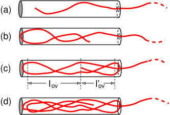
Figure 10: Illustration of the backfolding domains present for the data of $\kappa$=15 in Fig. 9. Parts (a), (b), (c) and (d) show domains with 0, 1, 2 and 3 backfolds, respectively.

As noted above, for sufficiently high $\kappa$ the regions between the steps exhibit a linear variation of $F_{\rm c}$ with $m$. Furthermore, the slope of these linear regions increase as the number of backfolds increases. To illustrate this, we plot the difference $\Delta F^{*}_{\rm c}\equiv F_{\rm c}(m;L=50)-F_{\rm c}(m;L=\infty)$ in Fig. 9(b). The increase in the slopes for $\kappa=15$ is more clearly evident. Linear fits to each of these regions are shown as black line segments in the figure (shifted vertically for clarity). The slope of each fit, labeled in the figure, increases as the number of hairpin backfolds increases.

To explain the origin of the linear regions and the variation of the slope with the number of hairpins, we use a theoretical approach that we previously employed to explain backfolding of semiflexible polymers in infinitely long channels.Polson et al. (2017); Polson (2018) This model relies on the Odijk regime condition that $P\gg D$, which is marginally satisfied for $\kappa$=15 and $D$=4. In the case of $L$=$\infty$ there is no backfolding and thus no overlap of the polymer along the tube. In this case the confinement free energy is proportional to the number of deflection segments, each of which contributes of order $kT$. Since the number of deflection segments is proportional to the number of translocated monomers, it follows that $F_{\rm c}\propto m$. In a backfolded regime where overlap is present, there are additional contributions to the free energy from the hairpin and excluded volume interactions between the deflection segments. After a complete hairpin is formed, increasing $m$ simply increases the degree of overlap. Modeling the deflection segments as hard rods of length $l_{\rm d}\sim D^{2/3}P^{1/3}$, the interaction free energy of $N$ such rods is $F_{\rm int}\approx l_{\rm d}^{2}wN^{2}\langle|\sin\gamma|\rangle/V$, where $V$ is the volume occupied by the segments and where the angle $\gamma$ between a pair rods satisfies $\langle|\sin\gamma|\rangle\approx D/l_{\rm d}$ in the case where they are highly aligned in the cylinder. The overlap volume can be written $V\sim l_{\rm ov}D^{2}$, where $l_{\rm ov}$ is the length of the overlap regime along the tube. Thus, the interaction free energy is $F_{\rm int}\sim l_{\rm d}wN^{2}/(l_{\rm ov}D^{2})$. Now, in a region where $F(m)$ is linear, there are two different overlap regions along the tube, one with $n$ overlapping strands and one with $n^{\prime}=n+1$ such strands, where $n$ is the number of hairpins present. The number of deflection segments in each region is $N=nl_{\rm ov}/l_{\rm d}$ and $N^{\prime}=(n+1)l^{\prime}_{\rm ov}/l_{\rm d}$, where $l_{\rm ov}$ and $l_{\rm ov}^{\prime}$ are the lengths of the two overlapping regions. (These lengths are illustrated in Fig. 10(c) for the case of $n$=2.) The total free energy arising from interacting segments from the two regions is

$$F_{\rm int}\sim\frac{l_{\rm d}wN^{2}}{l_{\rm ov}D}+\frac{l_{\rm d}w(N^{\prime})^{2}}{l^{\prime}_{\rm ov}D}$$ (7)

The overlap lengths are simply related by $l_{\rm ov}=L-2h_{z}-l^{\prime}_{\rm ov}$, where $h_{z}$ is the size of the hairpin along the channel. In addition, for a highly aligned polymer, $l^{\prime}_{\rm ov}\sim m$. Finally, noting that the Odijk deflection length scales as $l_{\rm d}\sim D^{2/3}P^{1/3}$, it is straightforward to show that Eq. (7) reduces to $F_{\rm int}\sim D^{-5/3}P^{-1/3}(2n+1)m$ plus terms independent of $m$. Thus, the contribution to the free-energy gradient from the excluded volume interactions is expected to scale as

$$f_{\rm int}\equiv\frac{dF_{\rm int}}{dm}\sim D^{-5/3}P^{-1/3}(2n+1)$$ (8)

Thus, $f_{\rm int}$ is predicted to increase with the number of hairpins, consistent with the observation in Fig. 9(b). For a quantitative comparison, we use Eq. (8) to estimate ratios of the gradients. We find that $f_{\rm int}(n=2)/f_{\rm int}(n=1)\approx 1.67$ and $f_{\rm int}(n=3)/f_{\rm int}(n=1)\approx 2.33$. By comparison, we find the corresponding ratios of the gradients in Fig. 9(b) are $0.281/0.143=1.96$ and $0.459/0.143=3.21$, respectively. Thus, the theoretical model underestimates the ratios of the gradients, and the discrepancy appears to grow as the number of hairpins increases. A similar discrepancy was observed using in Ref. Polson et al., 2017 for the ratios of overlap free-energy gradients of backfolded semiflexible polymers confined to long cylinders in the case where a single hairpin is present and the case of an S-loop with two hairpins. Likely origins of this discrepancy include not sufficiently satisfying the Odijk condition $P\gg D$, treating interactions at the second-virial level in a regime where the strands are tightly packed in a very narrow tube, and the neglect of correlations in position and orientation of deflection segments connected to the same hairpin.

Finally, it should be noted that the conformations characterized by multiple hairpins separated by elongated strands of Odijk deflection segments were observed here for the case where the persistence length $P$ is significantly less than the contour length $L_{\rm c}$ of the polymer, in addition to satisfying $P>D$. Recently, qualitatively different behaviour was observed in the case much stiffer polymers.Hayase et al. (2017) In the regime where $P\approx L_{\rm c}$, compression of a polymer in a finite-length channel resulted in the formation helical structures prior to the formation of hairpins. In the future, it would be of interest to examine the confinement free energy in this regime.

IV.5 Effects of Crowding Agents

We now investigate the effects of crowding agents on the free-energy functions for polymer translocation into confined cavities. For this purpose, we choose to employ symmetric cylindrical cavities (i.e. $D$=$L$) and consider first the case of monomer-sized crowding agents, i.e. $\sigma_{\rm c}$=$\sigma$=1. Figure  11 shows free-energy functions for translocation of a $N$=201 polymer into a cylindrical cavity of dimensions $D$$=$$L$=28 whose volume is partially occupied with $N_{\rm c}$ crowding agents, where $N_{\rm c}$ ranges from 0 to 4800, (i.e. crowder packing fractions up to $\phi_{\rm c}$=0.146). As expected, the free-energy cost for polymer insertion increases with increasing crowder density. The inset of the figure shows the excess free energy, which we define as $F_{\rm ex}(m)\equiv F(m;N_{\rm c})-F(m;N_{\rm c}=0)$; that is, $F_{\rm ex}(m)$ measures the variation of the free energy of the cavity/crowder system in excess of the variation in the free energy due to confinement alone, $F(m;N_{\rm c}=0)$. As is evident in the figure, $F_{\rm ex}$ varies linearly with $m$. Note that cavity size is such that $D/R_{\rm g}$=2.33, where $R_{\rm g}$ is the radius of gyration of a free polymer of the same size. For smaller values of $D/R_{\rm g}$, the same general trends are observed, though $F_{\rm ex}$ becomes increasingly less linear (data not shown).

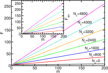
Figure 11: Free energy for translocation of a polymer of length $N$=201 into a cylindrical cavity of dimensions $D$=$L$=28 that is partially occupied by monomer-sized crowding agents. Results are shown for various values of the number of crowders, $N_{\rm c}$. The inset shows the corresponding excess free energy $F_{\rm ex}$ obtained from the translocation free-energy functions, where $F_{\rm ex}(m;N_{\rm c})\equiv F(m;N_{\rm c})-F(m;N_{\rm c}=0)$.

Figure 12 shows the variation of the excess insertion free energy for complete polymer insertion, $\Delta F_{\rm ex}\equiv F_{\rm ex}(m=N)$, vs crowding packing fraction $\phi_{\rm c}$ for $N$=201 and isotropic cavities with $D$=$L$. Results are shown for different cavity sizes with $D$ ranging from 10–28 (and thus $D/R_{\rm g}$=0.83–2.33). For each cavity size, $\Delta F_{\rm ex}$ increases monotonically with increasing crowder packing fraction. At any given packing fraction, the excess free energy decreases monotonically with increasing cavity size and appears to converge to a single curve for sufficiently large $D$. This is illustrated in the inset of the figure, which shows $\Delta F_{\rm ex}$ vs $D$ for a packing fraction of $\phi_{\rm c}$=0.1.

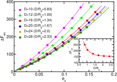
Figure 12: Excess free energy $\Delta F_{\rm ex}\equiv F_{\rm ex}(m=N)$ of inserting a polymer into a cavity partially occupied with crowding agents vs crowding agent packing fraction $\phi_{\rm c}$. We employ monomer-sized crowders, i.e. $\sigma_{\rm c}$=1, a polymer of length $N$=201, and a cylindrical cavity with $D$=$L$. Results are shown for several different cavity sizes, each labeled in the figure in relation to the radius of gyration $R_{\rm g}$ for a free polymer. The inset shows the variation of $\Delta F_{\rm ext}^{*}$ with $D$, where $\Delta F_{\rm ext}^{*}\equiv\Delta F_{\rm ex}(\phi_{\rm c}=0.1)$.

Figure 13(a) shows the variation of $\Delta F_{\rm ex}$ with $\phi_{\rm c}$ for $N$=201 and cavities with dimensions $D$=$L$=28. Results are shown for different crowder sizes in the range $\sigma_{\rm c}=$1.0–2.0. For each $\sigma_{\rm c}$ considered, $\Delta F_{\rm ex}$ increases with increasing $\phi_{\rm c}$. More significantly, at fixed crowder packing fraction, the excess free energy decreases monotonically with increasing crowder size. The effect is quite pronounced, as is also evident in the inset which shows $\Delta F_{\rm ex}$ vs $\sigma_{\rm c}$ for various packing fractions.

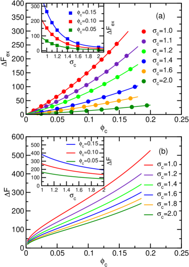
Figure 13: (a) Excess free energy $\Delta F_{\rm ex}\equiv F_{\rm ex}(m=N)$ of inserting a polymer into a cavity partially occupied with crowding agents vs crowding agent packing fraction $\phi_{\rm c}$. Results are shown for several values of the crowder size diameter $\sigma_{\rm c}$ for a polymer of length $N$=201 and a cylindrical cavity of dimensions $D$=14 and $L$=28. The inset shows $\Delta F_{\rm ex}$ vs $\sigma_{\rm c}$ for three different packing fractions using interpolations of the data in the main part of the figure. (b) Prediction of free-energy difference $\Delta F=F(m=N)-F(m=0)$ vs $\phi_{\rm c}$ using Eq. (9). The inset shows the prediction for $\Delta F$ vs $\sigma_{\rm c}$ for various packing fractions using Eq. (9).

The results in Fig. 13(a) are relevant to the simulation study by Chen and Luo.Chen and Luo (2013) In that work, the rate of translocation was examined for a polymer translocating between two spaces each occupied with crowding agents of different sizes but with equal packing fractions. They observed that a polymer initially configured with its center monomer in the nanopore tends to translocate into the space with the larger crowding agents. Note that the range of packing fractions and crowder sizes they considered ($\phi_{\rm c}$=0.05–0.4, $\sigma_{\rm c}$=1–2.5) are comparable to that examined here. However, since they used a 2-D system, a direct quantitative comparison with our results is not possible. Nevertheless, their observation is qualitatively consistent with our calculations, which predict a lower free energy for larger crowders at fixed $\phi_{\rm c}$ and thus a free-energy gradient that will drive translocation in that direction. Chen and Luo note, however, that the probability that the polymer goes to the high-$\sigma_{\rm c}$ side exhibits a maximum upon increasing $\sigma_{\rm c}$, and likewise the translocation rate exhibits a minimum. This is not consistent with trends evident in the free-energy calculations. Chen and Luo attribute this to kinetic effects due to “bottlenecks” related to the relative timescales of the conformational relaxation of the polymer and the diffusion of the obstacles. At low $\phi_{\rm c}$ and large $\sigma_{\rm c}$, this leads to “resisting force” of appreciable magnitude that effectively counteracts the entropic force, reducing the likelihood that the polymer reaches the higher-$\sigma_{\rm c}$ side. As this is an out-of-equilibrium effect, our free-energy calculations cannot account for this behaviour. However, our results can be used to test the analytical model used in Ref. Chen and Luo, 2013 to approximate the free-energy gradient.

In their theoretical model, Chen and Luo assume that this entropic force exerted by obstacles on either side of the nanopore scales $f\sim 1/R$, where $R$ is the mean spacing between the crowders. This assumption is inspired from a previous observation that a polymer ejected from a cylindrical nanochannel of diameter $R$ experiences a driving force with the same scaling. However, since a channel of fixed shape differs appreciably from the effective channels of fluctuating shape and size formed by the spaces between crowders, the accuracy of this prediction is not obvious a priori. Following the approach in Ref. Chen and Luo, 2013 and adapting it to a 3-D system, it is easily shown that the mean spacing between crowders is given by $R\approx(\pi/6\phi_{\rm c})^{1/3}\sigma_{\rm c}-\sigma_{\rm c}$. Noting that $f\propto dF/dm\propto 1/R$ and integrating with respect to $m$, it follows that

$$\Delta F\equiv F(N)-F(0)\propto\frac{N}{(\pi/6\phi_{\rm c})^{1/3}\sigma_{\rm c}-\sigma_{\rm c}}.$$ (9)

Figure 13(b) shows the predicted variation of $\Delta F$ with $\sigma_{\rm c}$ and (in the inset) with $\phi_{\rm c}$. Comparing the prediction with the simulation data reveals that the theory correctly predicts the qualitative trends, i.e. $\Delta F$ increases monotonically with increasing $\phi_{\rm c}$ for arbitrary crowder size, and it decreases monotonically with increasing $\sigma_{\rm c}$ for arbitrary packing fraction. As expected, however, the quantitative accuracy is very poor. It significantly overestimates the rate of increase in $\Delta F$ with $\phi_{\rm c}$ at low $\phi_{\rm c}$, and it significantly underestimates the rate of decrease in $\Delta F$ with increasing crowder size. Doubtless, the main cause of the discrepancy is the assumption that $f\sim 1/R$.

V Conclusions

In this study, we have used computer simulations to measure the free energy of a polymer undergoing translocation through a nanopore into a confining cavity. The scaling properties of the confinement free energy were examined with respect to the variation in several key system properties, including polymer length, cavity size and shape, polymer stiffness, and crowding from mobile crowding agents inside the cavity. These results complement and build on those of a previous study where we examined translocation into an ellipsoidal cavity.Polson (2015) The scaling results were typically compared with predictions obtained using standard scaling theories of polymer physics. While the measured scaling exponents are generally comparable to the predicted values, discrepancies arising from finite-size effects persist even for the longest polymer length employed here ($N$=601). A more rigorous test of the theoretical predictions in the future will likely require simulations employing polymer lengths at least an order of magnitude larger than is currently feasible. It will also be beneficial to consider other experimentally relevant factors such as the effects of electric driving forces and adsorption to the inner surface of the confining cavity.Rasmussen et al. (2012); Polson (2015) Clearly, in the absence of such forces the gradient in the free energy tends to drive the polymer out of the cavity. When present, however, they can provide a decrease in the potential energy as the monomers move inside the cavity that offsets or eliminates the loss in conformational entropy, thus driving the polymer inward.

Finally, it will be of interest to carry out additional simulations to measure and characterize the dynamics of polymer translocation into or out of confined cavities. For hard-sphere-chain polymers used here, either MC dynamicsPolson and McCaffrey (2013) or Discontinuous Molecular DynamicsOpps et al. (2013) simulations would be appropriate, while use of Brownian or Langevin dynamics techniques requires the use of continuous-potential models. A comparison of the rates of translocation into or out of the cavity with predictions from calculations employing the Fokker-Planck formalism will provide a means to delineate the regime in which translocation is a quasistatic process governed by the equilibrium free-energy function, as shown in previous work.Polson and McCaffrey (2013); Polson and Dunn (2014)