Dual Online Stein Variational Inference
for Control and Dynamics

Abstract

Model predictive control (MPC) schemes have a proven track record for delivering aggressive and robust performance in many challenging control tasks, coping with nonlinear system dynamics, constraints, and observational noise. Despite their success, these methods often rely on simple control distributions, which can limit their performance in highly uncertain and complex environments. MPC frameworks must be able to accommodate changing distributions over system parameters, based on the most recent measurements. In this paper, we devise an implicit variational inference algorithm able to estimate distributions over model parameters and control inputs on-the-fly. The method incorporates Stein Variational gradient descent to approximate the target distributions as a collection of particles, and performs updates based on a Bayesian formulation. This enables the approximation of complex multi-modal posterior distributions, typically occurring in challenging and realistic robot navigation tasks. We demonstrate our approach on both simulated and real-world experiments requiring real-time execution in the face of dynamically changing environments.

I Introduction

Real robotics applications are invariably subjected to uncertainty arising from either unknown model parameters or stochastic environments. To address the robustness of control strategies, many frameworks have been proposed of which model predictive control is one of the most successful and popular [5]. MPC has become a primary control method for handling nonlinear system dynamics and constraints on input, output and state, taking into account performance criteria. It originally gained popularity in chemical and processes control [11], being more recently adapted to various fields, such agricultural machinery [9], automotive systems [8], and robotics [16, 41]. In its essence, MPC relies on different optimisation strategies to find a sequence of actions over a given control horizon that minimises an optimality criteria defined by a cost function.

Despite their success in practical applications, traditional dynamic-programming approaches to MPC (such as iLQR and DDP [31]) rely on a differentiable cost function and dynamics model. Stochastic Optimal Control variants, such as iLQG [32] and PDDP [22], can accommodate stochastic dynamics, but only under simplifying assumptions such as additive Gaussian noise. These approaches are generally less effective in addressing complex distributions over actions, and it is unclear how these methods should incorporate model uncertainty, if any. In contrast, sampling-based control schemes have gained increasing popularity for their general robustness to model uncertainty, ease of implementation, and ability to contend with sparse cost functions [39].

To address some of these challenges, several approaches have been proposed. In sampling based Stochastic Optimal Control (SOC), the optimisation problem is replaced by a sampling-based algorithm that tries to approximate an optimal distribution over actions [38]. This has shown promising results in several applications and addresses some of the former disadvantages, however it may inadequately capture the complexity of the true posterior.

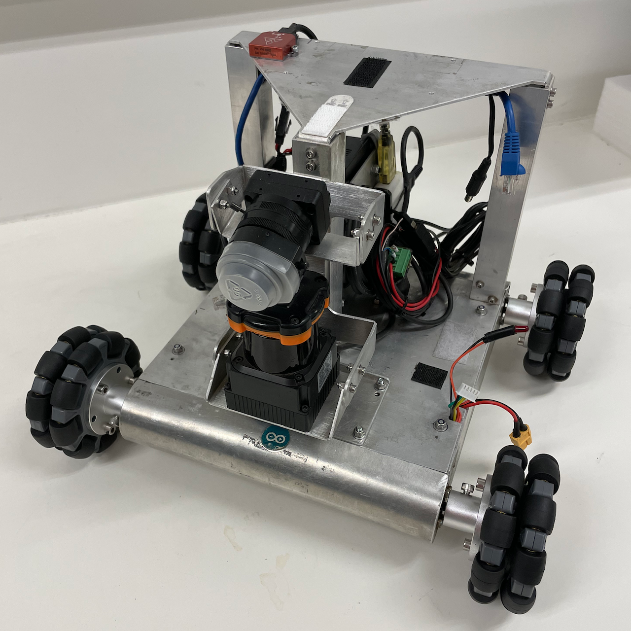
(a) Wombot AGV

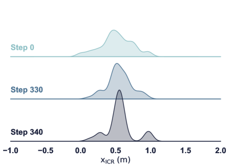
(b) Posterior distribution over $x_{{\operatorname{ICR}}}$

Figure 1: Online parameter estimation for autonomous ground vehicles. Distributions over system parameters such as the inertial center of rotation (ICR), are adapted in real-time. (a) The custom built skid-steer robot platform used in experiments. (b) Distribution over $x_{{\operatorname{ICR}}}$ at different time steps. The mass load on the robot is suddenly increased during system execution. The parameter distribution estimate quickly changes to include a second mode that better explains the new dynamics. Our particle-based control scheme can accommodate such multi-modal uncertainty and adapt to dynamically changing environments.

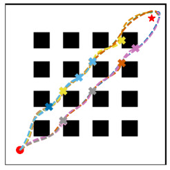
(a) SVMPC trajectories (baseline)

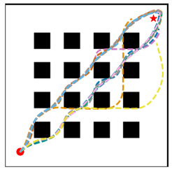
(b) DuSt-MPC trajectories (ours)

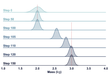
(c) Ridge plot of mass distribution (in kg)

Figure 2: Point-mass navigation task. The plots shows trajectories from the start position (red dot) towards the goal (red star). Left: Trajectories executed by SVMPC. Note that, as the mass of the robot changes, the model mismatch causes many of the episodes to crash (x markers). Centre: Trajectories executed by Dust-MPC. Depending on the state of the system when the mass change occurs, a few trajectories deviate from the centre path to avoid collisions. A few trajectories are truncated due to the fixed episode length. Right: Ridge plot of the distribution over mass along several steps of the simulation. The vertical dashed line denotes the true mass. Mass is initially set at 2 kg, and changed to 3 kg at step 100.

In recent work [18, 21], the MPC problem has been formulated as a Bayesian inference task whose goal is to estimate the posterior distribution over control parameters given the state and observed costs. To make such problem tractable in real-world applications, variational inference has been used to approximate the optimal distribution. These approaches are better suited at handling the multi-modality of the distribution over actions, but do not attempt to dynamically adapt to changes in the environment.

Conversely, previous work has demonstrated that incorporating uncertainty in the evaluation of SOC estimates can improve performance [2], particularly when this uncertainty is periodically re-estimated  [25]. Although this method is more robust to model mismatch and help address the sim-to-real gap, the strategy relies on applying moment-matching techniques to propagate the uncertainty through the dynamical system which is approximated by a Gaussian distribution. This diminishes the effectiveness of the method under settings where multi-modality is prominent.

In this work, we aim to leverage recent developments in variational inference with MPC for decision-making under complex multi-modal uncertainty over actions while simultaneously estimating the uncertainty over model parameters. We propose a Stein variational stochastic gradient solution that models the posterior distribution over actions and model parameters as a collection of particles, representing an implicit variational distribution. These particles are updated sequentially, online, in parallel, and can capture complex multi-modal distributions.

Specifically, the main contributions of this paper are:

• We propose a principled Bayesian solution of introducing uncertainty over model parameters in Stein variational MPC and empirically demonstrate how this can be leveraged to improve the control policy robustness;

• We introduce a novel method to extend the inference problem and simultaneously optimise the control policy while refining our knowledge of the environment as new observations are gathered. Crucially, by leveraging recent advancements in sequential Monte Carlo with kernel embedding, we perform online, sequential updates to the distribution over model parameters which scales to large datasets;

• By capturing the uncertainty on true dynamic systems in distributions over a parametric model, we are able to incorporate domain knowledge and physics principles while still allowing for a highly representative model. This simplifies the inference problem and drastically reduces the number of interactions with the environment to characterise the model.

We implement the algorithm on a real autonomous ground vehicle (AGV) (fig. 1(a)), illustrating the applicability of the method in real time. Experiments show how the control and parameter inference are leveraged to adapt the behaviour of the robot under varying conditions, such as changes in mass. We also present simulation results on an inverted pendulum and an 2D obstacle grid, see fig. 2, demonstrating an effective adaptation to dynamic changes in model parameters.

This paper is organised as follows. In Section II we review related work, contrasting the proposed method to the existing literature. In Section III we provide background on stochastic MPC and Stein variational gradient descent as a foundation to the proposed method, which is presented in Section IV. In Section V we present a number of real and simulated experiments, followed by relevant conclusions in Section VI.

II Related Work

Sampling-based approaches for stochastic MPC have shown to be suitable for a range of control problems in robotics [37, 35]. At each iteration, these methods perform an approximate evaluation by rolling-out a stochastic policy with modelled system dynamics over a finite-length horizon. The optimisation step proceeds to update the policy parameters in the direction that minimises the expected cost and a statistical distance to a reference policy or prior [35]. This can equivalently be interpreted as a statistical inference procedure, where policy parameters are updated in order to match an optimal posterior distribution distribution [28, 37, 18]. This connection has motivated the use of common approximate inference procedures for SOC. Model Predictive Path Integral Control (MPPI) [38, 37] and the Cross Entropy Method (CEM) [4], for instance, use importance sampling to match a Gaussian proposal distribution to moments of the posterior. Variational inference (VI) approaches have also been examined for addressing control problems exhibiting highly non-Gaussian or multi-modal posterior distributions. This family of Bayesian inference methods extends the modelling capacity of control distribution to minimise a Kullback-Leibler divergence with the target distribution. Traditional VI methods such as Expectation-Maximisation have been examined for control problems [36, 21], where the model class of the probability distribution is assumed to be restricted to a parametric family (typically Gaussian Mixture Models). More recently, the authors in  [18] proposed to adapt the Stein Variational Gradient Descent (SVGD) [20] method for model predictive control. Here, a distribution of control sequences is represented as a collection of particles. The resulting framework, Stein-Variational Model Predictive Control (SVMPC), adapts the particle distribution in an online fashion. The non-parametric representation makes the approach particularly suitable to systems exhibiting multi-modal posteriors. In the present work, we build on the approach in  [18] to develop an MPC framework which leverages particle-based variational inference to optimise controls and explicitly address model uncertainty. Our method simultaneously adapts a distribution over dynamics parameters, which we demonstrate improves robustness and performance on a real system.

Model predictive control is a reactive control scheme, and can accommodate modelling errors to a limited degree. However, its performance is largely affected by the accuracy of long-range predictions. Modelling errors can compound over the planning horizon, affecting the expected outcome of a given control action. This can be mitigated by accounting for model uncertainty, leading to better estimates of expected cost. This has been demonstrated to improve performance in stochastic optimal control methods and model-based reinforcement learning [22, 7]. Integrating uncertainty has typically been achieved by learning probabilistic dynamics models from collected state-transition data in an episodic setting, where the model is updated in between trajectory-length system executions [6, 21, 34, 27]. A variety of modelling representations have been explored, including Gaussian processes [7], neural network ensembles [6], Bayesian regression, and meta-learning [15]. Alternatively, the authors in [27, 25] estimate posterior distributions of physical parameters for black-box simulators, given real-world observations.

Recent efforts have examined the online setting, where a learned probabilistic model is updated based on observations made during execution [23, 1, 12, 13]. The benefits of this paradigm are clear: incorporating new observations and adapting the dynamics in situ will allow for better predictions, improved control, and recovery from sudden changes to the environment. However, real-time requirements dictate that model adaptation must be done quickly and efficiently, and accommodate the operational timescale of the controller. This typically comes at the cost of modelling accuracy, and limits the application of computationally-burdensome representations, such as neural networks and vanilla GPs. Previous work has included the use of sparse-spectrum GPs and efficient factorization to incrementally update the dynamics model  [23, 24]. In [15], the authors use a meta-learning approach to train a network model offline, which is adapted to new observations using Bayesian linear regression operating on the last layer. However, these approaches are restricted to Gaussian predictive distributions, and may lack sufficient modelling power for predicting complex, multi-modal distributions.

Perhaps most closely related to our modeling approach is the work by Abraham et al. [1]. The authors propose to track a distribution over simulation parameters using a sequential Monte Carlo method akin to a particle filter. The set of possible environments resulting from the parameter distribution is used by an MPPI controller to generate control samples. Each simulated trajectory rollout is then weighted according to the weight of the corresponding environment parameter. Although such an approach can model multi-modal posterior distributions, we should expect similar drawbacks to particle filters, which require clever re-sampling schemes to avoid mode collapse and particle depletion. Our method also leverages a particle-based representation of parameter distributions, but performs deterministic updates based on new information and is more sample efficient than MC sampling techniques.

III Background

III-A Stochastic Model Predictive Control

We consider the problem of controlling a discrete-time nonlinear system compactly represented as:

$${\bm{\mathbf{x}}}_{t+1}=f({\bm{\mathbf{x}}}_{t},{\bm{\mathbf{u}}}_{t})$$ (1)

where $f$ is the transition map, ${\bm{\mathbf{x}}}_{t}\in{\mathcal{{X}}}$ denotes the system state, ${\bm{\mathbf{u}}}_{t}\in{\mathcal{{U}}}$ the control input, and ${\mathcal{{X}}}$ and ${\mathcal{{U}}}$ are respectively appropriate Euclidean spaces for the states and controls. More specifically, we are interested in the problem where the real transition function $f({\bm{\mathbf{x}}}_{t},{\bm{\mathbf{u}}}_{t})$ is unknown and approximated by a transition function with parametric uncertainty, such that:

$$f({\bm{\mathbf{x}}}_{t},{\bm{\mathbf{u}}}_{t})\approx\hat{f}({\bm{\mathbf{x}}}_{t},{\bm{\mathbf{u}}}_{t},{\bm{\mathbf{\xi}}})=:\hat{f}_{{\bm{\mathbf{\xi}}}}({\bm{\mathbf{x}}}_{t},{\bm{\mathbf{u}}}_{t})$$ (2)

where ${\bm{\mathbf{\xi}}}\in\Xi$ are the simulator parameters with a prior probability distribution $p({\bm{\mathbf{\xi}}})$ and the non-linear forward model $\hat{f}({\bm{\mathbf{x}}},{\bm{\mathbf{u}}},{\bm{\mathbf{\xi}}})$, is represented as $\hat{f}_{{\bm{\mathbf{\xi}}}}$ for compactness.

Based on the steps in [2], we can then define a fixed length control sequence ${U}_{t}=\{{\bm{\mathbf{u}}}_{t}\}_{t<t+H}$ over a fixed control horizon $H$, onto which we apply a receding horizon control (RHC) strategy. Moreover, we define a mapping operator, $\mathcal{H}$, from input sequences ${U}_{t}$ to their resulting states by recursively applying $\hat{f}_{{\bm{\mathbf{\xi}}}}$ given ${\bm{\mathbf{x}}}_{t}$,

$$\begin{split}{X}_{t}&=\mathcal{H}({U}_{t};{\bm{\mathbf{x}}}_{t})\\ &=\left[{\bm{\mathbf{x}}}_{t},\hat{f}_{{\bm{\mathbf{\xi}}}}({\bm{\mathbf{x}}}_{t},{\bm{\mathbf{u}}}_{t}),\hat{f}_{{\bm{\mathbf{\xi}}}}(\hat{f}_{{\bm{\mathbf{\xi}}}}({\bm{\mathbf{x}}}_{t},{\bm{\mathbf{u}}}_{t}),{\bm{\mathbf{u}}}_{t+1}),\ldots\right]\,,\end{split}$$ (3)

noting that ${X}_{t}$ and ${U}_{t}$ define estimates of future states and controls. Finally, we can define a trajectory as the joint sequence of states and actions, namely:

$${\bm{\mathbf{\tau}}}=\left({X}_{t},{U}_{t}\right)\,.$$ (4)

In MPC, we want to minimise a task dependent cost functional generally described as:

$$C\left({X}_{t},{U}_{t}\right)=c_{term}(\hat{{\bm{\mathbf{x}}}}_{t+H})+\sum_{h=0}^{H-1}c(\hat{{\bm{\mathbf{x}}}}_{t+h},\hat{{\bm{\mathbf{u}}}}_{t+h})\,,$$ (5)

where $\hat{{\bm{\mathbf{x}}}}$ and $\hat{{\bm{\mathbf{u}}}}$ are the estimated states and controls, and $c(\cdot)$ and $c_{term}(\cdot)$ are respectively arbitrary instantaneous and terminal cost functions. To do so, our goal is to find an optimal policy $\pi({\bm{\mathbf{x}}}_{t})$ to generate the control sequence ${U}_{t}$ at each time-step. As in [35], we define such feedback policy as a parameterised probability distribution $\pi_{{\bm{\mathbf{\theta}}}_{t}}=p({\bm{\mathbf{u}}}_{t}|{\bm{\mathbf{x}}}_{t};{\bm{\mathbf{\theta}}}_{t})$ from which the actions at time $t$ are sampled, i.e. ${U}_{t}\sim\pi_{{\bm{\mathbf{\theta}}}_{t}}$. The control problem can then be defined as:

$$\min_{{\bm{\mathbf{\theta}}}_{t}\in\Theta}\hat{J}\left(\pi_{{\bm{\mathbf{\theta}}}_{t}};{\bm{\mathbf{x}}}_{t}\right)\,,$$ (6)

where $\hat{J}$ is an estimator for a statistic of interest, typically $\mathbb{E}_{\pi_{{\bm{\mathbf{\theta}}}_{t}},\hat{f}_{{\bm{\mathbf{\xi}}}}}\left[C\left({X}_{t},{U}_{t}\right)\right]$. Once $\pi_{{\bm{\mathbf{\theta}}}_{t}}$ is determined, we can use it to sample ${U}_{t}$, extract the first control ${\bm{\mathbf{u}}}_{t}$ and apply it to the system.

One of the main advantages of stochastic MPC is that $\hat{J}$ can be computed even when the cost function is non-differentiable w.r.t. to the policy parameters by using importance sampling [38].

III-B Stein Variational Gradient Descent

Variational inference poses posterior estimation as an optimisation task where a candidate distribution $q^{*}({\bm{\mathbf{x}}})$ within a distribution family ${\mathcal{{Q}}}$ is chosen to best approximate the target distribution $p({\bm{\mathbf{x}}})$. This is typically obtained by minimising the Kullback-Leibler (KL) divergence:

$$q^{*}({\bm{\mathbf{x}}})=\operatornamewithlimits{argmin}_{q\in{\mathcal{{Q}}}}\ D_{\mathrm{KL}}(q({\bm{\mathbf{x}}})||p({\bm{\mathbf{x}}}))\,.$$ (7)

The solution also maximises the Evidence Lower Bound (ELBO), as expressed by the following objective:

$$q^{*}({\bm{\mathbf{x}}})=\operatornamewithlimits{argmax}_{q\in{\mathcal{{Q}}}}\mathbb{E}_{q}[\log p({\bm{\mathbf{x}}})]-D_{\mathrm{KL}}(q({\bm{\mathbf{x}}})||p({\bm{\mathbf{x}}}))$$ (8)

In order to circumvent the challenge of determining an appropriate ${\mathcal{{Q}}}$, while also addressing eq. 7, we develop an algorithm based on Stein variational gradient descent (SVGD) for Bayesian inference [20]. The non-parametric nature of SVGD is advantageous as it removes the need for assumptions on restricted parametric families for $q({\bm{\mathbf{x}}})$. This approach approximates a posterior $p({\bm{\mathbf{x}}})$ with a set of particles $\{{\bm{\mathbf{x}}}^{i}\}_{i}^{N_{p}}$, ${\bm{\mathbf{x}}}\in p$. These particles are iteratively updated according to:

$${\bm{\mathbf{x}}}^{i}\leftarrow{\bm{\mathbf{x}}}^{i}+\epsilon{\bm{\mathbf{\phi}}}^{*}({\bm{\mathbf{x}}}^{i})\,,$$ (9)

given a step size $\epsilon$. The function $\phi(\cdot)$ is known as score function and defines the velocity field that maximally decreases the KL-divergence.

$${\bm{\mathbf{\phi}}}^{*}=\underset{{\bm{\mathbf{\phi}}}\in\mathcal{S}}{\operatornamewithlimits{argmax}}\left\{-\nabla_{\epsilon}D_{\mathrm{KL}}(q_{[\epsilon\phi]}||p({\bm{\mathbf{x}}})),\text{\leavevmode\nobreak\ s.t.\leavevmode\nobreak\ }\|{\bm{\mathbf{\phi}}}\|_{\mathcal{S}}\leq 1\right\}$$ (10)

where $\mathcal{S}$ is a Reproducing Kernel Hilbert Space (RKHS) induced by the kernel function used and $q_{[\epsilon\phi]}$ indicates the particle distribution resulting from taking an update step as in eq. 9. In [20] this has been shown to yield a closed-form solution which can be interpreted as a functional gradient in $\mathcal{S}$ and approximated with the set of particles:

$${{\bm{\mathbf{\phi}}}}^{*}({\bm{\mathbf{x}}})=\frac{1}{N_{p}}\sum_{j=1}^{N_{p}}\left[k({\bm{\mathbf{x}}}^{j},{\bm{\mathbf{x}}})\nabla_{{\bm{\mathbf{x}}}^{j}}\log p({\bm{\mathbf{x}}}^{j})+\nabla_{{\bm{\mathbf{x}}}^{j}}k({\bm{\mathbf{x}}}^{j},{\bm{\mathbf{x}}})\right]$$ (11)

IV Method

In this section, we present our approach for joint inference over control and model parameters for MPC. We call this method Dual Stein Variational Inference MPC, or DuSt-MPC for conciseness. We begin by formulating optimal control as an inference problem and address how to optimise policies in section IV-C. Later, in section IV-D, we extend the inference to also include the system dynamics. A complete overview of the method is described in algorithm in appendix A.

IV-A MPC as Bayesian Inference

MPC can be framed as a Bayesian inference problem where we estimate the posterior distribution of policies, parameterised by ${\bm{\mathbf{\theta}}}_{t}$, given an optimality criterion. Let $\mathcal{O}:{\mathcal{{T}}}\to\{0,1\}$ be an optimality indicator for a trajectory ${\bm{\mathbf{\tau}}}\in{\mathcal{{T}}}$ such that $\mathcal{O}[{\bm{\mathbf{\tau}}}]=1$ indicates that the trajectory is optimal. Now we can apply Bayes’ Rule and frame our problem as estimating:

$$p({\bm{\mathbf{\theta}}}_{t}|\mathcal{O})\propto p(\mathcal{O}|{\bm{\mathbf{\theta}}}_{t})p({\bm{\mathbf{\theta}}}_{t})=p(\mathcal{O},{\bm{\mathbf{\theta}}}_{t}).$$ (12)

A reasonable to way to quantify $\mathcal{O}[{\bm{\mathbf{\tau}}}]$ is to model it as a Bernoulli random variable conditioned on the trajectory ${\bm{\mathbf{\tau}}}$, allowing us to define the likelihood $p(\mathcal{O}|{\bm{\mathbf{\theta}}}_{t})$ as:

$$\begin{split}p(\mathcal{O}|{\bm{\mathbf{\theta}}}_{t})&=\mathbb{E}_{{\bm{\mathbf{\tau}}}\sim p({\bm{\mathbf{\tau}}}|{\bm{\mathbf{\theta}}}_{t})}\left[p(\mathcal{O}[{\bm{\mathbf{\tau}}}]=1|{\bm{\mathbf{\tau}}})\right]\\ &\approx\frac{1}{n}\sum_{i=1}^{n}\exp(-\alpha C[{\bm{\mathbf{\tau}}}_{i}])\,,\end{split}$$ (13)

where ${\bm{\mathbf{\tau}}}_{i}\overset{i.i.d.}{\sim}p({\bm{\mathbf{\tau}}}|{\bm{\mathbf{\theta}}}_{t})$, $i\in\{1,2,\dots,n\}$, $p(\mathcal{O}[{\bm{\mathbf{\tau}}}]=1|{\bm{\mathbf{\tau}}}):=\exp(-\alpha C[{\bm{\mathbf{\tau}}}])$, and we overload $p(\mathcal{O}[{\bm{\mathbf{\tau}}}]=1|{\bm{\mathbf{\theta}}}_{t})$ to simplify the notation. Now, assuming a prior $p({\bm{\mathbf{\theta}}}_{t})$ for ${\bm{\mathbf{\theta}}}_{t}$, the posterior over ${\bm{\mathbf{\theta}}}_{t}$ is given by:

$$\begin{split}p({\bm{\mathbf{\theta}}}_{t}|\mathcal{O})&\propto p(\mathcal{O}|{\bm{\mathbf{\theta}}}_{t})p({\bm{\mathbf{\theta}}}_{t})=\int_{\mathcal{{T}}}p(\mathcal{O}|{\bm{\mathbf{\tau}}})p({\bm{\mathbf{\tau}}}|{\bm{\mathbf{\theta}}}_{t})p({\bm{\mathbf{\theta}}}_{t}){\operatorname{d}}{\bm{\mathbf{\tau}}}\,.\end{split}$$ (14)

This posterior corresponds to the probability (density) of a given parameter setting ${\bm{\mathbf{\theta}}}_{t}$ conditioned on the hypothesis that (implicitly observed) trajectories generated by ${\bm{\mathbf{\theta}}}_{t}$ are optimal. Alternatively, one may say that $p({\bm{\mathbf{\theta}}}_{t}|\mathcal{O})$ tells us the probability of ${\bm{\mathbf{\theta}}}_{t}$ being the generator of the optimal set ${\mathcal{{T}}}^{*}$. Lastly, note that the trajectories conditional $p({\bm{\mathbf{\tau}}}|{\bm{\mathbf{\theta}}}_{t})$ factorises as:

$$p({\bm{\mathbf{\tau}}}|{\bm{\mathbf{\theta}}}_{t})=\prod_{h=0}^{H-1}p_{\bm{\mathbf{\xi}}}({\bm{\mathbf{x}}}_{t+h+1}|{\bm{\mathbf{x}}}_{t+h},{\bm{\mathbf{u}}}_{t+h})\pi_{{\bm{\mathbf{\theta}}}_{t}}({\bm{\mathbf{x}}}_{t+h})\,.$$ (15)

IV-B Joint Inference for Policy and Dynamics with Stein MPC

In this section, we generalise the framework presented in [18] to simultaneously refine our knowledge of the dynamical system, parameterised by ${\bm{\mathbf{\xi}}}$, while estimating optimal policy parameters ${\bm{\mathbf{\theta}}}_{t}$. Before we proceed, however, it is important to notice that the optimality measure defined in section IV-A stems from simulated rollouts sampled according to eq. 13. Hence, these trajectories are not actual observations of the agent’s environment and are not suitable for inferring the parameters of the system dynamics. In other words, to perform inference over the parameters ${\bm{\mathbf{\xi}}}$ we need to collect real observations from the environment.

With that in mind, the problem statement in eq. 12 can be rewritten as inferring:

$$p({\bm{\mathbf{\theta}}}_{t},{\bm{\mathbf{\xi}}}|\mathcal{O},\mathcal{D}_{1:t})=p({\bm{\mathbf{\theta}}}_{t}|\mathcal{O},{\bm{\mathbf{\xi}}})p({\bm{\mathbf{\xi}}}|\mathcal{D}_{1:t})\,,$$ (16)

where $\mathcal{D}_{1:t}:=\{({\bm{\mathbf{x}}}_{t}^{r},{\bm{\mathbf{u}}}_{t-1}^{r},{\bm{\mathbf{x}}}_{t-1}^{r})\}_{t=1}^{N_{\mathcal{D}}}$ represents the dataset of collected environment observations. Note that the policy parameters ${\bm{\mathbf{\theta}}}$ are independent from the system observations, and therefore the conditioning on $\mathcal{D}_{1:t}$ has been dropped. Similarly, the distribution over dynamics parameters is independent from $\mathcal{O}$ and again we omit the conditioning.

The reader might wonder why we have factorised eq. 16 instead of defining a new random variable $\Theta=\{{\bm{\mathbf{\theta}}},{\bm{\mathbf{\xi}}}\}$, and following the steps outlined in [18] to solve the joint inference problem. By jointly solving the inference problem the partial derivative of ${\bm{\mathbf{\xi}}}$ would be comprised of terms involving both factors on the right-hand side (RHS) of eq. 16, biasing the estimation of ${\bm{\mathbf{\xi}}}$ to regions of lower control cost (see appendix D for further discussion). Furthermore, the two inference problems are naturally disjoint. While the policy inference relies on simulated future rollouts, the dynamics inference is based solely on previously observed data.

By factorising the problem we can perform each inference step separately and adjust the computational effort and hyper-parameters based on the idiosyncrasies of the problem at hand. This formulation is particularly amenable for stochastic MPC, as seen in section III, since the policy $\pi_{{\bm{\mathbf{\theta}}}_{t}}$ is independent of the approximated transition function $\hat{f}_{{\bm{\mathbf{\xi}}}}$, i.e. ${\bm{\mathbf{\theta}}}\perp\!\!\!\perp{\bm{\mathbf{\xi}}}$.

IV-C Policy Inference for Bayesian MPC

Having formulated the inference problem as in eq. 16, we can proceed by solving each of the factors separately. We shall start with optimising $\pi_{{\bm{\mathbf{\theta}}}_{t}}$ according to $p({\bm{\mathbf{\theta}}}_{t}|\mathcal{O},{\bm{\mathbf{\xi}}})$. It is evident that we need to consider the dynamics parameters when optimising the policy, but at this stage we may simply assume the inference over ${\bm{\mathbf{\xi}}}$ has been solved and leverage our knowledge of $p({\bm{\mathbf{\xi}}}|\mathcal{D}_{1:t})$. More concretely, let us rewrite the factor on the RHS of eq. 16 by marginalising over ${\bm{\mathbf{\xi}}}$ so that:

$$p({\bm{\mathbf{\theta}}}_{t}|\mathcal{O},\mathcal{D}_{1:t})\propto\int_{\Xi}\ell_{\pi}({\bm{\mathbf{\theta}}}_{t})p({\bm{\mathbf{\theta}}}_{t})p({\bm{\mathbf{\xi}}}|\mathcal{D}_{1:t}){\operatorname{d}}{\bm{\mathbf{\xi}}}\,,$$ (17)

where, as in eq. 13, the likelihood $\ell_{\pi}({\bm{\mathbf{\theta}}}_{t})$ is defined as:

$$\begin{split}\ell_{\pi}({\bm{\mathbf{\theta}}}_{t})&=p(\mathcal{O}|{\bm{\mathbf{\theta}}}_{t},{\bm{\mathbf{\xi}}}):=P({\mathcal{{T}}}^{*}|{\bm{\mathbf{\theta}}}_{t},{\bm{\mathbf{\xi}}})\\ &=\int_{\mathcal{{T}}}p(\mathcal{O}|{\bm{\mathbf{\tau}}})p({\bm{\mathbf{\tau}}}|{\bm{\mathbf{\theta}}}_{t},{\bm{\mathbf{\xi}}}){\operatorname{d}}{\bm{\mathbf{\tau}}}\\ &\approx\frac{1}{N_{{\bm{\mathbf{\tau}}}}}\sum_{i=1}^{N_{{\bm{\mathbf{\tau}}}}}\exp(-\alpha C[{\bm{\mathbf{\tau}}}_{i}])\,,\end{split}$$ (18)

with ${\bm{\mathbf{\tau}}}_{i}\overset{i.i.d.}{\sim}p({\bm{\mathbf{\tau}}}|{\bm{\mathbf{\theta}}}_{t},{\bm{\mathbf{\xi}}})$, $i\in\{1,2,\dots,N_{{\bm{\mathbf{\tau}}}}\}$, and $p({\bm{\mathbf{\xi}}}|\mathcal{D}_{1:t})$ defines the inference problem of updating the posterior distribution of the dynamics parameters given all observations gathered from the environment, which we shall discuss in the next section. Careful consideration of eq. 18 tells us that unlike the case of a deterministic transition function or even maximum likelihood point estimation of ${\bm{\mathbf{\xi}}}$, the optimality of a given trajectory now depends on its expected cost over the distribution $p({\bm{\mathbf{\xi}}})$.

Hence, given a prior $p({\bm{\mathbf{\theta}}}_{t})$ and $p({\bm{\mathbf{\xi}}}|\mathcal{D}_{1:t})$, we can generate samples from the likelihood in eq. 18 and use an stochastic gradient method as in section III-B to infer the posterior distribution over ${\bm{\mathbf{\theta}}}_{t}$. Following the steps in [18], we approximate the prior $p({\bm{\mathbf{\theta}}}_{t})$ by a set of particles $q({\bm{\mathbf{\theta}}}_{t})=\{{\bm{\mathbf{\theta}}}_{t}\}_{i=1}^{N_{\pi}}$ and take sequential SVGD updates:

$${\bm{\mathbf{\theta}}}_{t}^{i}\leftarrow{\bm{\mathbf{\theta}}}_{t}^{i}+\epsilon{\bm{\mathbf{\phi}}}^{*}({\bm{\mathbf{\theta}}}_{t}^{i})\,,$$ (19)

to derive the posterior distribution. Where, again, ${\bm{\mathbf{\phi}}}^{*}$ is computed as in eq. 11 for each intermediate step and $\epsilon$ is a predetermined step size. One ingredient missing to compute the score function is the gradient of the log-posterior of $p({\bm{\mathbf{\theta}}}_{t}|\mathcal{O},{\bm{\mathbf{\xi}}})$, which can be factorised into:

$$\nabla_{{\bm{\mathbf{\theta}}}_{t}^{i}}\log p({\bm{\mathbf{\theta}}}_{t}^{i}|\mathcal{O},{\bm{\mathbf{\xi}}})=\nabla_{{\bm{\mathbf{\theta}}}_{t}^{i}}\log\ell({\bm{\mathbf{\theta}}}_{t}^{i})+\nabla_{{\bm{\mathbf{\theta}}}_{t}^{i}}\log q({\bm{\mathbf{\theta}}}_{t}^{i})\,.$$ (20)

In practice we typically assume that the $C[\cdot]$ functional used as surrogate for optimality is not differentiable w.r.t. ${\bm{\mathbf{\theta}}}_{t}$, but the gradient of the log-likelihood can be usually approximated via Monte-Carlo sampling.

Most notably, however, is the fact that unlike the original formulation in SVGD, the policy distribution we are trying to infer is time-varying and depends on the actual state of the system. The measure $P({\mathcal{{T}}}^{*}|{\bm{\mathbf{\theta}}}_{t};{\bm{\mathbf{x}}}_{t})$ depends on the current state, as that is the initial condition for all trajectories evaluated in the cost functional $C[{\bm{\mathbf{\tau}}}]$.

Theoretically, one could choose an uninformative prior with broad support over the ${\mathcal{{U}}}$ at each time-step and employ standard SVGD to compute the posterior policy. However, due to the sequential nature of the MPC algorithm, it is likely that the prior policy $q({\bm{\mathbf{\theta}}}_{t-1})$ is close to a region of low cost and hence is a good candidate to bootstrap the posterior inference of the subsequent step. This procedure is akin to the prediction step commonly found in Sequential Bayesian Estimation [10]. More concretely,

$$q({\bm{\mathbf{\theta}}}_{t})=\int p({\bm{\mathbf{\theta}}}_{t}|{\bm{\mathbf{\theta}}}_{t-1})q({\bm{\mathbf{\theta}}}_{t-1}){\operatorname{d}}{\bm{\mathbf{\theta}}}_{t-1}\,,$$ (21)

where $p({\bm{\mathbf{\theta}}}_{t}|{\bm{\mathbf{\theta}}}_{t-1})$ can be an arbitrary transitional probability distribution. More commonly, however, is to use a probabilistic version of the shift operator as defined in [35]. For a brief discussion on action selection, please refer to appendix B. For more details on this section in general the reader is encouraged to refer to [18, Sec. 5.3].

IV-D Real-time Dynamics Inference

We now focus on the problem of updating the posterior over the simulator parameters. Note that, due to the independence of each inference problem, the frequency in which we update $p({\bm{\mathbf{\xi}}})$ can be different from the policy update.

In contrast, we are interested in the case where $p({\bm{\mathbf{\xi}}}|\mathcal{D}_{1:t})$ can be updated in real-time adjusting to changes in the environment. For that end, we need a more efficient way of updating our posterior distribution. The inference problem at a given time-step can then be written as:

$$\begin{split}p({\bm{\mathbf{\xi}}}|\mathcal{D}_{1:t})&\propto p(\mathcal{D}_{t}|{\bm{\mathbf{\xi}}},\mathcal{D}_{1:t-1})p({\bm{\mathbf{\xi}}}|\mathcal{D}_{1:t-1})\,.\end{split}$$ (22)

Note that in this formulation, ${\bm{\mathbf{\xi}}}$ is considered time-invariant. This based on the implicit assumption that the frequency in which we gather new observations is significantly larger than the covariate shift to which $p({\bm{\mathbf{\xi}}}|\mathcal{D}_{1:t})$ is subject to as we traverse the environment. In appendix C, we discuss the implications of changes in the the latent parameter over time.

In general, we do not have access to direct measurements of ${\bm{\mathbf{\xi}}}$, only to the system state. Therefore, in order to perform inference over the dynamics parameters, we rely on a generative model, i.e. the simulator $\hat{f}_{{\bm{\mathbf{\xi}}}}$, to generate samples in the state space ${\mathcal{{X}}}$ for different values of ${\bm{\mathbf{\xi}}}$. However, unlike in the policy inference step, for the dynamics parameter estimation we are not computing deterministic simulated rollouts, but rather trying to find the explanatory parameter for each observed transition in the environment. Namely, we have:

$${\bm{\mathbf{x}}}^{r}_{t}=f({\bm{\mathbf{x}}}^{r}_{t-1},{\bm{\mathbf{u}}}_{t-1})=\hat{f}_{{\bm{\mathbf{\xi}}}}({\bm{\mathbf{x}}}^{r}_{t-1},{\bm{\mathbf{u}}}_{t-1})+{\eta}_{t}\,,$$ (23)

where ${\bm{\mathbf{x}}}^{r}_{t}$ denotes the true system state and ${\eta}_{t}$ is a time-dependent random variable closely related to the reality gap in the sim-to-real literature [33] and incorporates all the complexities of the real system not captured in simulation, such as model mismatch, unmodelled dynamics, etc. As result, the distribution of ${\eta}_{t}$ is unknown, correlated over time and hard to estimate.

In practice, for the feasibility of the inference problem, we make the standard assumption that the noise is distributed according to a time-invariant normal distribution ${\eta}_{t}\sim\mathcal{N}(0,{{\Sigma}}_{\operatorname{obs}})$, with an empirically chosen covariance matrix. More concretely, this allows us to define the likelihood term in eq. 22 as:

$$\begin{split}\ell({\bm{\mathbf{\xi}}}|\mathcal{D}_{1:t})&:=p(\mathcal{D}_{t}|{\bm{\mathbf{\xi}}},\mathcal{D}_{1:t-1})\\ &=p({\bm{\mathbf{x}}}^{r}_{t}|{\bm{\mathbf{\xi}}},\mathcal{D}_{1:t-1})\\ &=\mathcal{N}({\bm{\mathbf{x}}}^{r}_{t};\hat{f}_{{\bm{\mathbf{\xi}}}}({\bm{\mathbf{x}}}^{r}_{t-1},{\bm{\mathbf{u}}}_{t-1}),{{\Sigma}}_{\operatorname{obs}})\,,\end{split}$$ (24)

where we leverage the symmetry of the Gaussian distribution to centre the uncertainty around ${\bm{\mathbf{x}}}^{r}_{t}$. It follows that, because the state transition is Markovian, the likelihood of $\ell({\bm{\mathbf{\xi}}}|\mathcal{D}_{1:t})$ depends only on the current observation tuple given by $\mathcal{D}_{t}$, and we can drop the conditioning on previously observed data. In other words, we now have a way to quantify how likely is a given realisation of ${\bm{\mathbf{\xi}}}$ based on the data we have collected from the environment. Furthermore, let us define a single observation $\mathcal{D}_{t}=({\bm{\mathbf{x}}}_{t}^{r},{\bm{\mathbf{u}}}_{t-1}^{r},{\bm{\mathbf{x}}}_{t-1}^{r})$ as the tuple of last applied control action and observed state transition. Inferring exclusively over the current state is useful whenever frequent observations are received and prevents us from having to store information over the entire observation dataset. This approach is also followed by ensemble Kalman filters and particle flow filters [19].

Equipped with eq. 24 and assuming that an initial prior $p({\bm{\mathbf{\xi}}})$ is available, we can proceed as discussed in section III-B by approximating each prior at time $t$ with a set of particles $\{{\bm{\mathbf{\xi}}}^{i}\}_{i=1}^{N_{\bm{\mathbf{\xi}}}}$ following $q({\bm{\mathbf{\xi}}}|\mathcal{D}_{1:t-1})$, so that our posterior over ${\bm{\mathbf{\xi}}}$ at a given time $t$ can then be rewritten as:

$$p({\bm{\mathbf{\xi}}}|\mathcal{D}_{1:t})\approx q({\bm{\mathbf{\xi}}}|\mathcal{D}_{1:t})\propto\ell({\bm{\mathbf{\xi}}}|\mathcal{D}_{t})q({\bm{\mathbf{\xi}}}|\mathcal{D}_{1:t-1})\,,$$ (25)

and we can make recursive updates to $q({\bm{\mathbf{\xi}}}|\mathcal{D}_{1:t})$ by employing it as the prior distribution for the following step. Namely, we can iteratively update $q({\bm{\mathbf{\xi}}}|\mathcal{D}_{1:t})$ a number of steps $L$ by applying the update rule with a functional gradient computed as in eq. 11, where:

$$\nabla_{{\bm{\mathbf{\xi}}}}\log p_{t}({\bm{\mathbf{\xi}}}|\mathcal{D}_{1:t})\approx\nabla_{{\bm{\mathbf{\xi}}}}\log p(\mathcal{D}_{t}|{\bm{\mathbf{\xi}}})+\nabla_{{\bm{\mathbf{\xi}}}}\log q_{t}({\bm{\mathbf{\xi}}}|\mathcal{D}_{1:t})\,.$$ (26)

An element needed to evaluate eq. 26 is an expression for the gradient of the posterior density. An issue in sequential Bayesian inference is that there is no exact expression for the posterior density [26]. Namely, we know the likelihood function, but the prior density is only represented by a set of particles, not the density itself.

One could forge an empirical distribution $q({\bm{\mathbf{\xi}}}|\mathcal{D}_{1:t})=\frac{1}{{N_{\bm{\mathbf{\xi}}}}}\sum_{i=1}^{N_{\bm{\mathbf{\xi}}}}\delta({\bm{\mathbf{\xi}}}^{i})$ by assigning Dirac functions at each particle location, but we would still be unable to differentiate the posterior. In practice, we need to apply an efficient density estimation method, as we need to compute the density at each optimisation step. We choose to approximate the posterior density with an equal-weight Gaussian Mixture Model (GMM) with a fixed diagonal covariance matrix:

$$q({\bm{\mathbf{\xi}}}|\mathcal{D}_{1:t})=\frac{1}{{N_{\bm{\mathbf{\xi}}}}}\sum_{i=1}^{N_{\bm{\mathbf{\xi}}}}\mathcal{N}({\bm{\mathbf{\xi}}};{\bm{\mathbf{\xi}}}^{i},{{\Sigma}}_{\operatorname{s}})\,,$$ (27)

where the covariance matrix ${{\Sigma}}_{\operatorname{s}}$ can be predetermined or computed from data. One option, for example, is to use a Kernel Density bandwidth estimation heuristic, such as Improved Sheather Jones [3], Silverman’s [30] or Scott’s [29] rule, to determine the standard deviation $\sigma$ and set ${{\Sigma}}_{\operatorname{s}}=\sigma^{2}{{I}}$.

One final consideration is that of the support for the prior distribution. Given the discussion above, it is important that the density approximation of $q({\bm{\mathbf{\xi}}}|\mathcal{D}_{t})$ offers support on regions of interest in the parameter space. In our formulation, that can be controlled by adjusting ${{\Sigma}}_{\operatorname{s}}$. Additionally, precautions have to be taken to make sure the parameter space is specified correctly, such as using log-transformations for strictly positive parameters for instance.

V Experiments

In the following section we present experiments, both in simulation and with a physical autonomous ground vehicle (AGV), to demonstrate the correctness and applicability of our method.

V-A Inverted pendulum with uncertain parameters

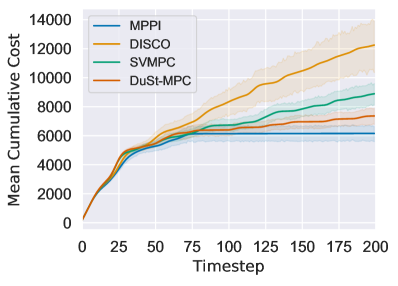
(a) Pendulum costs

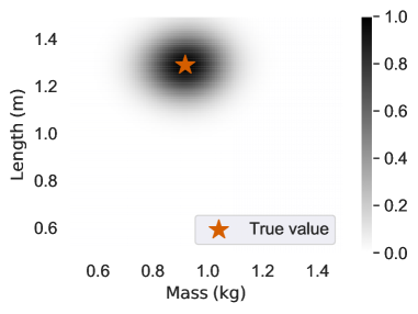
(b) Pendulum posterior

Figure 3: Inverted pendulum. (a) The image shows the mean cumulative cost over 10 episodes. The shaded region represents the 50% confidence interval. The high variance is expected since each scenario has parameters sampled from a uniform distribution. (b) Plot of the posterior distribution over the pendulum pole-mass at the final step of one of the episodes. The true latent value is shown by the red star marker.

We first investigate the performance of DuSt-MPC in the classic inverted pendulum control problem. As usual, the pendulum is composed of a rigid pole-mass system controlled at one end by a 1-degree-of-freedom torque actuator. The task is to balance the point-mass upright, which, as the controller is typically under-actuated, requires a controlled swing motion to overcome gravity. Contrary to the typical case, however, in our experiments the mass and length of the pole-mass are unknown and equally likely within a range of $0.5\text{\,}\mathrm{kg}1.5\text{\,}\mathrm{kg}$ and $0.5\text{\,}\mathrm{m}1.5\text{\,}\mathrm{m}$, respectively.

At each episode, a set of latent model parameters is sampled and used in the simulated environment. Each method is then deployed utilising this same parameter set. MPPI is used as a baseline and has perfect knowledge of the latent parameters. This provides a measure of the task difficulty and achievable results. As discussed in section II, we compare against DISCO and SVMPC as additional baselines. We argue that, although these methods perform no online update of their knowledge of the world, they offer a good underpinning for comparison since the former tries to leverage the model uncertainty to create more robust policies, whereas the latter shares the same variational inference principles as our method. DISCO is implemented in its unscented transform variant applied to the uninformative prior used to generate the random environments. SVMPC uses the mean values for mass and length as point-estimates for its fixed parametric model. For more details on the hyper-parameters used, refer to appendix E.

Figure 3(a) presents the average cumulative costs over 10 episodes. Although the results show great variance, due to the randomised environment, it is clear that DuSt-MPC outperforms both baselines. Careful consideration will show that the improvement is more noticeable as the episode progresses, which is expected as the posterior distribution over the model parameters being used by DuSt-MPC gets more informative. The final distribution over mass and length for one of the episodes is shown in fig. 3(b). Finally, a summary of the experimental results is presented in table I.

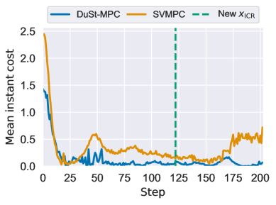
(a) Raw costs

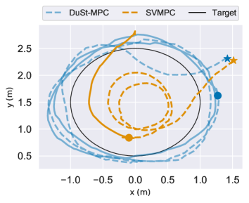
(b) Trajectories

Figure 4: AGV trajectory tracking. (a) Raw cost over time. Amount of steps before and after the change of mass are normalised for proper comparison. (b) Trajectories executed by each method. Line style changes when mass changes. Markers denote initial and change of mass position.

	Point-mass		Pendulum
	Cost $(\mu\pm\sigma)$	Succ.†	Cost $(\mu\pm\sigma)$	Succ.‡
MPPI§	—	—	$30.8\pm 12.6$	100%
DISCO	$250.8\pm 29.9$	20%	$61.3\pm 40.0$	70%
SVMPC	$191.7\pm 56.5$	25%	$44.5\pm 17.9$	70%
DuSt-MPC	$\mathbf{118.3\pm 07.9}$	100%	$\mathbf{36.8\pm 14.0}$	80%

Table I: Simulation results. Summary of results for simulation experiments. The mean episode cost is given by the sum of the instant costs over the episode length. Values shown do not include the crash penalty for a more comparable baseline. ^§Not used in the navigation task; has perfect knowledge in the pendulum task. ^†Successes are episodes with no crashes. ^‡Successes are episodes whose last five steps have a instant cost below 4 ($\approx$$10\mathrm{°}$ from the upright position).

V-B Point-mass navigation on an obstacle grid

Here, we reproduce and extend the planar navigation task presented in [18]. We construct a scenario in which an holonomic point-mass robot must reach a target location while avoiding obstacles. As in [18], colliding with obstacles not only incurs a high cost penalty to the controller, but prevents all future movement, simulating a crash. The non-differentiable cost function makes this a challenging problem, well-suited for sampling-based approaches. Obstacles lie in an equally spaced 4-by-4 grid, yielding several multi-modal solutions. This is depicted in fig. 2. Additionally, we include barriers at the boundaries of the simulated space to prevent the robot from easily circumventing obstacles.

The system dynamics is represented as a double integrator model with non-unitary mass $m$, s.t. the particle acceleration is given by $\ddot{{\bm{\mathbf{x}}}}=m^{-1}{\bm{\mathbf{u}}}$ and the control signal is the force applied to the point-mass. In order to demonstrate the inference over dynamics, we forcibly change the mass of the robot at a fixed step of the experiment, adding extra weight. This has a direct parallel to several tasks in reality, such as collecting a payload or passengers while executing a task. Assuming the goal position is denoted by ${\bm{\mathbf{x}}}_{g}$, the cost function that defines the task is given by:

$$\begin{split}&c({\bm{\mathbf{x}}}_{t},{\bm{\mathbf{u}}}_{t})=0.5{\bm{\mathbf{e}}}_{t}^{\mathsf{T}}{\bm{\mathbf{e}}}_{t}+0.25\dot{{\bm{\mathbf{x}}}_{t}}^{\mathsf{T}}\dot{{\bm{\mathbf{x}}}_{t}}+0.2{\bm{\mathbf{u}}}_{t}^{\mathsf{T}}{\bm{\mathbf{u}}}_{t}+p\cdot\bm{\mathbb{1}}\{\operatorname{col.}\}\\ &c_{term}({\bm{\mathbf{x}}}_{t},{\bm{\mathbf{u}}}_{t})=1000{\bm{\mathbf{e}}}_{t}^{\mathsf{T}}{\bm{\mathbf{e}}}_{t}+0.1\dot{{\bm{\mathbf{x}}}_{t}}^{\mathsf{T}}\dot{{\bm{\mathbf{x}}}_{t}}\,,\end{split}$$

where ${\bm{\mathbf{e}}}_{t}={\bm{\mathbf{x}}}_{t}-{\bm{\mathbf{x}}}_{g}$ is the instantaneous position error and $p=10^{6}$ is the penalty when a collision happens. A detailed account of the hyper-parameters used in the experiment is presented in appendix E.

As a baseline, we once more compare against DISCO and SVMPC. In fig. 2 we present an overlay of the trajectories for SVMPC and DuSt-MPC over 20 independent episodes and we choose to omit trajectories of DISCO for conciseness. Collisions to obstacles are denoted by a x marker. Note that in a third of the episodes SVMPC is unable to avoid obstacles due to the high model mismatch while DuSt-MPC is able to avoid collisions by quickly adjusting to the new model configuration online. A typical sequential plot of the posterior distribution induced by fitting a GMM as in eq. 27 is shown on fig. 2(c) for one episode. There is little variation between episodes and the distribution remains stable in the intermediate steps not depicted.

V-C Trajectory tracking with autonomous ground vehicle

We now present experimental results with a physical autonomous ground robot equipped with a skid-steering drive mechanism. The kinematics of the robot are based on a modified unicycle model, which accounts for skidding via an additional parameter [17]. The parameters of interest in this model are the robot’s wheel radius $r_{{\operatorname{w}}}$, axial distance $a_{{\operatorname{w}}}$, i.e. the distance between the wheels, and the displacement of the robot’s ICR from the robot’s centre $x_{{\operatorname{ICR}}}$. A non-zero value on the latter affects turning by sliding the robot sideways. The robot is velocity controlled and, although it possess four-wheel drive, the controls is restricted to two-degrees of freedom, left and right wheel speed. Individual wheel speeds are regulated by a low-level proportional-integral controller.

The robot is equipped with a 2D Hokuyo LIDAR and operates in an indoor environment in our experiments. Prior to the tests, the area is pre-mapped using the gmapping package [14] and the robot is localised against this pre-built map. Similar to the experiment in section V-B, we simulate a change in the environment that could be captured by our parametric model of the robot to explain the real trajectories. However, we are only applying a relatively simple kinematic model in which the effects of the dynamics and ground-wheel interactions are not accounted for. Therefore, friction and mass are not feasible inference choices. Hence, out of the available parameters, we opted for inferring $x_{{\operatorname{ICR}}}$, the robot’s centre of rotation. Since measuring $x_{{\operatorname{ICR}}}$ involves a laborious process, requiring different weight measurements or many trajectories from the physical hardware [40], this also makes the experiment more realistic. To circumvent the difficulties of ascertaining $x_{{\operatorname{ICR}}}$, we use the posterior distribution estimated in [2], and bootstrap our experiment with $x_{{\operatorname{ICR}}}\sim\mathcal{N}(0.5,0.2^{2})$.

To reduce the influence of external effects, such as localisation, we defined a simple control task of following a circular path at a constant tangential speed. Costs were set to make the robot follow a circle of $1\text{\,}\mathrm{m}$ radius with $c({\bm{\mathbf{x}}}_{t})=\sqrt{d_{t}^{2}+10(s_{t}-s_{0})^{2}}$, where $d_{t}$ represents the robot’s distance to the edge of the circle and $s_{0}=$0.2\text{\,}\mathrm{m}\text{\,}{\mathrm{s}}^{-1}$$ is a reference linear speed.

The initial particles needed by DuSt-MPC in eq. 26 for the estimation of $x_{{\operatorname{ICR}}}$ are sampled from the bootstrapping distribution, whereas for SVMPC we set $x_{{\operatorname{ICR}}}=$0.5\text{\,}\mathrm{m}$$, the distribution mean. Again, we want to capture whether our method is capable of adjusting to environmental changes. To this end, approximately halfway through the experiment, we add an extra load of approximately $5.3\text{\,}\mathrm{kg}$ at the rear of the robot in order to alter its centre of mass. These moments are indicated on the trajectories shown in fig. 4(b). In fig. 4(a) we plot the instant costs for a fixed number of steps before and after the change of mass. For the complete experiment parameters refer to the appendix E.

We observe that considering the uncertainty over $x_{{\operatorname{ICR}}}$ and, crucially, refining our knowledge over it (see fig. 1(b) in appendix E), allows DuSt-MPC to significantly outperform the SVMPC baseline. Focusing on the trajectories from SVMPC we note that our estimation of $x_{{\operatorname{ICR}}}$ is probably not accurate. As the cost function emphasises the tangential speed over the cross-track error, this results in circles correctly centred, but of smaller radius. Crucially though, the algorithm cannot overcome this poor initial estimation. DuSt-MPC initially appears to find the same solution, but quickly adapts, overshooting the target trajectory and eventually converging to a better result. This behaviour can be observed both prior to and after the change in the robot’s mass. Conversely, with the addition of mass, the trajectory of SVMPC diverged and eventually led the robot to a halt.

VI Conclusions

We present a method capable of simultaneously estimating model parameters and controls. The method expands previous results in control as implicit variational inference and provides the theoretical framework to formally incorporate uncertainty over simulator parameters. By encapsulating the uncertainty on dynamic systems as distributions over a parametric model, we are able to incorporate domain knowledge and physics principles while still allowing for a highly representative model. Crucially, we perform an online refinement step where the agent leverages system feedback in a sequential way to efficiently update its beliefs regardless of the size of observation dataset.

Simulated experiments are presented for a randomised inverted pendulum environment and obstacle grid with step changes in the dynamical parameters. Additionally, a trajectory tracking experiment utilising a custom built AGV demonstrates the feasibility of the method for online control. The results illustrate how the simplifications on dynamic inference are effective and allow for a quick adjustment of the posterior belief resulting in a de facto adaptive controller. Consider, for instance, the inverted pendulum task. In such periodic and non-linear system, untangling mass and length can pose a difficult challenge as there are many plausible solutions [27]. Nonetheless, the results obtained are quite encouraging, even with very few mapping steps per control loop.

Finally, we demonstrated how, by incorporating uncertainty over the model parameters, DuSt-MPC produces more robust policies to dynamically changing environments, even when the posterior estimation of the model parameters is rather uncertain. This can be seen, for instance, in the adjustments made to trajectories in the obstacle grid.

Appendix A Algorithm

1

2Sample $\left\{{\bm{\mathbf{\theta}}}_{t_{0}}^{i}\right\}_{i=1}^{{N_{\pi}}}\sim q({\bm{\mathbf{\theta}}}_{t_{0}})$

3foreach policy $i\in{N_{\pi}}$ do $\pi_{{\bm{\mathbf{\theta}}}^{i}}\leftarrow\mathcal{N}({\bm{\mathbf{\theta}}}_{t_{0}}^{i},{{\Sigma}}_{\operatorname{a}})$

4

5while task not complete do

6       ${\bm{\mathbf{x}}}_{t}^{r}\leftarrow$ GetStateEstimate()

7      $\mathcal{D}_{1:t}\leftarrow\mathcal{D}_{1:t-1}\bigcup\{{\bm{\mathbf{x}}}_{t}^{r},{\bm{\mathbf{x}}}_{t-1}^{r},{\bm{\mathbf{u}}}_{t-1}^{r}$}

8      for $l\leftarrow 1$ to $L$ do // Dynamics inference loop

9             for $m\leftarrow 1$ to ${N_{\bm{\mathbf{\xi}}}}$ do

                   $\ell({\bm{\mathbf{\xi}}}|\mathcal{D}_{1:t})\leftarrow\mathcal{N}(\hat{f}_{{\bm{\mathbf{\xi}}}}({\bm{\mathbf{x}}}^{r}_{t-1},{\bm{\mathbf{u}}}_{t-1}^{r});{\bm{\mathbf{x}}}^{r}_{t},{{\Sigma}}_{\operatorname{obs}})$

                    // Condition likelihood, eq. 24

10                  

                  $\nabla_{{\bm{\mathbf{\xi}}}}\log p({\bm{\mathbf{\xi}}}^{m}|\mathcal{D}_{1:t})\approx\nabla_{{\bm{\mathbf{\xi}}}}\log\ell({\bm{\mathbf{\xi}}}^{m}|\mathcal{D}_{1:t})+\nabla_{{\bm{\mathbf{\xi}}}}\log q({\bm{\mathbf{\xi}}}^{m}|\mathcal{D}_{1:t-1})$

                    // eq. 26

11                  

                  ${\bm{\mathbf{\phi}}}({\bm{\mathbf{\xi}}}^{m})\leftarrow\frac{1}{{N_{\bm{\mathbf{\xi}}}}}\sum_{j=1}^{{N_{\bm{\mathbf{\xi}}}}}k({\bm{\mathbf{\xi}}}^{j},{\bm{\mathbf{\xi}}}^{m})\nabla_{{\bm{\mathbf{\xi}}}}\log p_{t}({\bm{\mathbf{\xi}}}^{m}|\mathcal{D}_{1:t})+\nabla_{{\bm{\mathbf{\xi}}}}k({\bm{\mathbf{\xi}}}^{j},{\bm{\mathbf{\xi}}}^{m})$

                    // Stein gradient, eq. 11

12                  

13                  ${\bm{\mathbf{\xi}}}^{m}\leftarrow{\bm{\mathbf{\xi}}}^{m}+\epsilon{\bm{\mathbf{\phi}}}({\bm{\mathbf{\xi}}}^{m})$

                  $q({\bm{\mathbf{\xi}}}|\mathcal{D}_{1:t})=\frac{1}{{N_{\bm{\mathbf{\xi}}}}}\sum_{m=1}^{N_{\bm{\mathbf{\xi}}}}\mathcal{N}({\bm{\mathbf{\xi}}}^{m},{{\Sigma}}_{\operatorname{s}})$

                    // Update posterior, eq. 27

14                  

15             end for

16            

17       end for

18      Sample $\left\{{\bm{\mathbf{\xi}}}^{m}\right\}_{m=1}^{{N_{\bm{\mathbf{\xi}}}}}\sim q({\bm{\mathbf{\xi}}}|\mathcal{D}_{1:t})$

19      for $i\leftarrow 1$ to ${N_{\pi}}$ do // Policies inference loop

20             Sample $\left\{{U}_{n}^{i}\right\}_{n=1}^{N_{\operatorname{a}}}\sim\pi_{{\bm{\mathbf{\theta}}}^{i}}$

21            foreach $n\in N_{\operatorname{a}}$ and $m\in N_{\operatorname{s}}$ do $C_{n,m}^{i}\leftarrow$ GetRolloutCosts$({U}_{n}^{i},{\bm{\mathbf{\xi}}}^{m},{\bm{\mathbf{x}}}_{t}^{r})$

22              // eqs. 3 and 5

            $\nabla_{{\bm{\mathbf{\theta}}}}\log p({\bm{\mathbf{\theta}}}_{t}^{i}|\mathcal{O},{\bm{\mathbf{\xi}}})\approx\nabla_{{\bm{\mathbf{\theta}}}}\log q({\bm{\mathbf{\theta}}}_{t-1}^{i})+\nabla_{{\bm{\mathbf{\theta}}}}\log\left(\frac{1}{N_{\operatorname{a}}N_{\operatorname{s}}}\sum_{n=1}^{N_{\operatorname{a}}}\sum_{m=1}^{N_{\operatorname{s}}}\exp(-\alpha C_{n,m}^{i})\right)$

              // eq. 20

23            

            ${\bm{\mathbf{\phi}}}({\bm{\mathbf{\theta}}}_{t}^{i})\leftarrow\frac{1}{{N_{\pi}}}\sum_{j=1}^{{N_{\pi}}}k({\bm{\mathbf{\theta}}}_{t-1}^{j},{\bm{\mathbf{\theta}}}_{t}^{i})\nabla_{{\bm{\mathbf{\theta}}}}\log p({\bm{\mathbf{\theta}}}_{t}^{j}|\mathcal{O},{\bm{\mathbf{\xi}}})+\nabla_{{\bm{\mathbf{\theta}}}}k({\bm{\mathbf{\theta}}}_{t}^{j},{\bm{\mathbf{\theta}}}_{t}^{i})$

              // Stein gradient

24            

25            ${\bm{\mathbf{\theta}}}_{t}^{i}\leftarrow{\bm{\mathbf{\theta}}}_{t}^{i}+\epsilon{\bm{\mathbf{\phi}}}({\bm{\mathbf{\theta}}}_{t}^{i})$

            $\omega_{t}^{i}\leftarrow\frac{q({\bm{\mathbf{\theta}}}_{t-1}^{i})}{N_{\operatorname{a}}N_{\operatorname{s}}}\sum_{n=1}^{N_{\operatorname{a}}}\sum_{m=1}^{N_{\operatorname{s}}}\exp(-\alpha C_{n,m}^{i})$

              // Compute weights, eq. 28

26            

27       end for

28      foreach policy $i\in{N_{\pi}}$ do $\omega_{t}^{i}\leftarrow\frac{\omega_{t}^{i}}{\sum_{i=1}^{{N_{\pi}}}\omega_{t}^{i}}$

29      

30      $i^{*}=\operatornamewithlimits{argmax}_{i}{\omega_{t}^{i}}$

      SendToActuators$({U}_{t}^{i^{*}}={\bm{\mathbf{\theta}}}_{t}^{i^{*}})$

        // Applies first action of the control sequence

31      

      ${\bm{\mathbf{\theta}}}_{t}\leftarrow$ RollPolicies$({\bm{\mathbf{\theta}}}_{t})$

        // Shift one step ahead, adds noise to last step

32      

      $q({\bm{\mathbf{\theta}}}_{t})=\sum_{i=1}^{{N_{\pi}}}\omega_{t}^{i}\mathcal{N}({\bm{\mathbf{\theta}}}_{t}^{i},{{\Sigma}})$

        // Update policies prior, eq. 21

33      

34      foreach policy $i\in{N_{\pi}}$ do $\pi_{{\bm{\mathbf{\theta}}}^{i}}\leftarrow\mathcal{N}({\bm{\mathbf{\theta}}}_{t}^{i},{{\Sigma}}_{\operatorname{a}})$

35      

36      $t\leftarrow t+1$

37 end while

Algorithm 1 Sim-to-Real in the loop SVMPC

Appendix B Considerations on Action Selection

Once policy parameters have been updated according to eq. 19, we can update the policy for the current step, $\pi_{{\bm{\mathbf{\theta}}}_{t}}$. However, defining the updated policy is not enough, as we still need to determine which immediate control action should be sent to the system. There are many options which could be considered at this stage. One alternative would be to take the expected value at each time-step, although that could compromise the multi-modality of the solution found. Other options would be to consider the modes $\pi_{{\bm{\mathbf{\theta}}}_{t}}$ of at each horizon step or sample the actions directly. Finally, we adopt the choice of computing the probabilistic weight of each particle and choosing the highest weighted particle as the action sequence for the current step. More formally:

$$\omega_{i}=\frac{p(\mathcal{O}|{\bm{\mathbf{\theta}}}_{t}^{i},{\bm{\mathbf{\xi}}})q({\bm{\mathbf{\theta}}}_{t-1}^{i})}{\sum_{j=1}^{m}p(\mathcal{O}|{\bm{\mathbf{\theta}}}_{t}^{j},{\bm{\mathbf{\xi}}})q({\bm{\mathbf{\theta}}}_{t-1}^{j})}\approx p({\bm{\mathbf{\theta}}}_{t}^{i}|\mathcal{O},{\bm{\mathbf{\xi}}})\,.$$ (28)

And finally, the action deployed to the system would be given by ${U}_{t}^{i^{*}}={\bm{\mathbf{\theta}}}_{t}^{i^{*}}$, where $i^{*}=\operatornamewithlimits{argmax}_{i}{\omega_{t}^{i}}$.

Appendix C Considerations on Covariate Shift

The proposed inference method assumes that the parameters of the dynamical model are fixed over time. Note that, even if the distribution over parameters changes over time, this remains a plausible consideration, given that the control loop will likely have a relatively high frequency when compared to the environment covariate shift. This also ensures that trajectories generated in simulation are consistent and that the resulting changes are being governed by the variations in the control actions and not the environment.

However, it is also clear that the method is intrinsically adaptable to changes in the environment, as long as there is a minimum probability of the latent parameter being feasible under the prior distribution $q({\bm{\mathbf{\xi}}}|\mathcal{D}_{t})$. Too see this, consider the case where there is an abrupt change in the environment (e.g. the agent picks-up some load or the type of terrain changes). In this situation, $q({\bm{\mathbf{\xi}}}|\mathcal{D}_{t-1})$ would behave as if a poorly specified prior, meaning that as long the probability density around the true distribution $p({\bm{\mathbf{\xi}}})$ is non-zero, we would still converge to the true distribution, albeit requiring further gradient steps.

In practice, the more data we gather to corroborate a given parameter set, the more concentrated the distribution would be around a given location in the parameter space and the longer it would take to transport the probability mass to other regions of the parameter space. This could be controlled by including heuristic weight terms to the likelihood and prior in eq. 22. However, we deliberately choose not to include extra hyper-parameters based on the hypothesis that the control loop is significantly faster than the changes in the environment, which in general allows the system to gather a few dozens or possibly more observations before converging to a good estimate of ${\bm{\mathbf{\xi}}}$.

Appendix D Bias on joint inference of policy and dynamics

Note that, if we take the gradient of eq. 16 w.r.t. ${\bm{\mathbf{\xi}}}$, we get:

$$\begin{split}\nabla_{{\bm{\mathbf{\xi}}}}p({\bm{\mathbf{\theta}}}_{t},{\bm{\mathbf{\xi}}}|\mathcal{O},\mathcal{D}_{1:t})&=\nabla_{{\bm{\mathbf{\xi}}}}\left[p({\bm{\mathbf{\theta}}}_{t}|\mathcal{O},{\bm{\mathbf{\xi}}})p({\bm{\mathbf{\xi}}}|\mathcal{D}_{1:t})\right]\\ &=p({\bm{\mathbf{\xi}}}|\mathcal{D}_{1:t})\nabla_{{\bm{\mathbf{\xi}}}}p({\bm{\mathbf{\theta}}}_{t}|\mathcal{O},{\bm{\mathbf{\xi}}})+p({\bm{\mathbf{\theta}}}_{t}|\mathcal{O},{\bm{\mathbf{\xi}}})\nabla_{{\bm{\mathbf{\xi}}}}p({\bm{\mathbf{\xi}}}|\mathcal{D}_{1:t})\,.\end{split}$$ (29)

The first term on the RHS of the equation above indicates that the optimality gradient of simulated trajectories would contribute to the update of ${\bm{\mathbf{\xi}}}$. Although this is true for the policy updates, we don’t want the inference of the physical parameters to be biased by our optimality measure. In other words, the distribution over ${\bm{\mathbf{\xi}}}$ shouldn’t conform to whatever would benefit the optimality policy, but the other way around.

Appendix E Further details on performed experiments

Parameter	Inverted Pendulum	Point-mass Navigation	AGV Traj. Tracking
Initial state, ${\bm{\mathbf{x}}}_{0}$	[$3\text{\,}\mathrm{rad}$, $0\text{\,}\mathrm{m}\mathrm{/}\sec$]	—	—
Environment maximum speed	$5\text{\,}\mathrm{m}\mathrm{/}\sec$	—	—
Environment maximum acceleration	$10\text{\,}\mathrm{m}\mathrm{/}\sec\mathrm{{}^{2}}$	—	—
Policy samples, $N_{\operatorname{a}}$	$32$	$64$	$50$
Dynamics samples, $N_{\operatorname{s}}$	$8$	$4$	$4$
Cost Likelihood inverse temperature, $\alpha$	$1.0$	$1.0$	$1.0$
Control authority, ${{\Sigma}}$	$2.0^{2}$	$5.0^{2}$	$0.1^{2}$
Control horizon, $H$	$20$	$40$	$20$
Number of policies, ${N_{\pi}}$	$3$	$6$	$2$
Policy Kernel, $k_{\pi}(\cdot,\cdot)$	Radial Basis Function
Policy Kernel bandwidth selection	Silverman’s rule
Policy prior covariance, ${{\Sigma}}_{\operatorname{a}}$	$2.0^{2}$	$5.0^{2}$	$1.0^{2}$
Policy step size, $\epsilon$	$2.0$	$100.0$	$0.02$
Dynamics prior distribution
Dynamics number of particles, ${N_{\bm{\mathbf{\xi}}}}$	$50$	$50$	$50$
Dynamics Kernel, $k_{{\bm{\mathbf{\xi}}}}(\cdot,\cdot)$	Radial Basis Function
Dynamics GMM covariance, ${{\Sigma}}_{\operatorname{s}}$	Improved Sheather Jones	$0.25^{2}$	$0.0625^{2}$
Dynamics likelihood covariance, ${{\Sigma}}_{\operatorname{obs}}$	$0.1^{2}$	$0.1^{2}$	$0.1^{2}$
Dynamics update steps, $L$	$20$	$20$	$5$
Dynamics step size, $\epsilon$	$0.001$	$0.01$	$0.05$
Dynamics in log space	No	Yes	No
Unscented Transform spread [2], $\alpha$	$0.5$	—	—

Table II: Hyperparameters used in the experiments.

References

- [1] Ian Abraham et al. “Model-Based Generalization Under Parameter Uncertainty Using Path Integral Control” In IEEE Robotics and Automation Letters 5.2 IEEE, 2020, pp. 2864–2871
- [2] Lucas Barcelos et al. “DISCO: Double Likelihood-Free Inference Stochastic Control” In Proceedings of the 2020 IEEE International Conference on Robotics and Automation Paris, France: IEEE RoboticsAutomation Society, 2020, pp. 7 DOI: 978-1-7281-7395-5/20
- [3] Z.. Botev, J.. Grotowski and D.. Kroese “Kernel Density Estimation via Diffusion” In The Annals of Statistics 38.5 Institute of Mathematical Statistics, 2010, pp. 2916–2957 DOI: 10.1214/10-AOS799
- [4] Zdravko I Botev, Dirk P Kroese, Reuven Y Rubinstein and Pierre L’Ecuyer “The cross-entropy method for optimization” In Handbook of statistics 31 Elsevier, 2013, pp. 35–59
- [5] Eduardo F. Camacho and Carlos Bordons Alba “Model Predictive Control”, Advanced Textbooks in Control and Signal Processing London: Springer-Verlag, 2013 URL: https://www.springer.com/gp/book/9780857293985
- [6] Kurtland Chua, Roberto Calandra, Rowan McAllister and Sergey Levine “Deep Reinforcement Learning in a Handful of Trials using Probabilistic Dynamics Models” In arXiv:1805.12114 [cs, stat], 2018 arXiv: http://arxiv.org/abs/1805.12114
- [7] Marc Peter Deisenroth and Carl Edward Rasmussen “PILCO: A Model-Based and Data-Efficient Approach to Policy Search”, pp. 8
- [8] Stefano Di Cairano and Ilya V Kolmanovsky “Automotive applications of model predictive control” In Handbook of Model Predictive Control Springer, 2019, pp. 493–527
- [9] Ying Ding, Liang Wang, Yongwei Li and Daoliang Li “Model predictive control and its application in agriculture: A review” In Computers and Electronics in Agriculture 151 Elsevier, 2018, pp. 104–117
- [10] Arnaud Doucet “Sequential Monte Carlo Methods in Practice”, 2001 URL: https://doi.org/10.1007/978-1-4757-3437-9
- [11] John W Eaton and James B Rawlings “Model-predictive control of chemical processes” In Chemical Engineering Science 47.4 Elsevier, 1992, pp. 705–720
- [12] David Fan, Ali Agha and Evangelos Theodorou “Deep Learning Tubes for Tube MPC” In Robotics: Science and Systems XVI Robotics: ScienceSystems Foundation, 2020 DOI: 10.15607/RSS.2020.XVI.087
- [13] Jaime F. Fisac et al. “A General Safety Framework for Learning-Based Control in Uncertain Robotic Systems” In IEEE Transactions on Automatic Control 64.7, 2019, pp. 2737–2752 DOI: 10.1109/TAC.2018.2876389
- [14] Giorgio Grisetti, Cyrill Stachniss and Wolfram Burgard “Improved techniques for grid mapping with rao-blackwellized particle filters” In IEEE transactions on Robotics 23.1 IEEE, 2007, pp. 34–46
- [15] James Harrison, Apoorva Sharma and Marco Pavone “Meta-learning priors for efficient online bayesian regression” In International Workshop on the Algorithmic Foundations of Robotics, 2018, pp. 318–337 Springer
- [16] Mina Kamel, Thomas Stastny, Kostas Alexis and Roland Siegwart “Model predictive control for trajectory tracking of unmanned aerial vehicles using robot operating system” In Robot operating system (ROS) Springer, 2017, pp. 3–39
- [17] Krzysztof Kozłowski and Dariusz Pazderski “Modeling and Control of a 4-wheel Skid-steering Mobile Robot” In Int. J. Appl. Math. Comput. Sci. 14.4, 2004, pp. 477–496
- [18] Alexander Lambert et al. “Stein Variational Model Predictive Control” In Proceedings of the 4th Annual Conference on Robot Learning, 2020
- [19] Peter Jan Leeuwen et al. “Particle Filters for High-dimensional Geoscience Applications: A Review” In Q.J.R. Meteorol. Soc. 145.723, 2019, pp. 2335–2365 DOI: 10.1002/qj.3551
- [20] Qiang Liu and Dilin Wang “Stein Variational Gradient Descent: A General Purpose Bayesian Inference Algorithm” In arXiv:1608.04471 [cs, stat], 2019 arXiv: http://arxiv.org/abs/1608.04471
- [21] Masashi Okada and Tadahiro Taniguchi “Variational Inference MPC for Bayesian Model-based Reinforcement Learning” In arXiv:1907.04202 [cs, eess, stat], 2019 arXiv: http://arxiv.org/abs/1907.04202
- [22] Yunpeng Pan and Evangelos Theodorou “Probabilistic differential dynamic programming” In Advances in Neural Information Processing Systems 27, 2014, pp. 1907–1915
- [23] Yunpeng Pan, Xinyan Yan, Evangelos Theodorou and Byron Boots “Adaptive probabilistic trajectory optimization via efficient approximate inference” In 29th Conference on Neural Information Processing System, 2016
- [24] Yunpeng Pan, Xinyan Yan, Evangelos A. Theodorou and Byron Boots “Prediction under uncertainty in sparse spectrum Gaussian processes with applications to filtering and control” tex.pdf: http://proceedings.mlr.press/v70/pan17a/pan17a.pdf In Proceedings of the 34th international conference on machine learning 70, Proceedings of machine learning research International Convention Centre, Sydney, Australia: PMLR, 2017, pp. 2760–2768 URL: http://proceedings.mlr.press/v70/pan17a.html
- [25] Rafael Possas et al. “Online BayesSim for Combined Simulator Parameter Inference and Policy Improvement”, 2020, pp. 8
- [26] Manuel Pulido and Peter Jan Leeuwen “Sequential Monte Carlo with kernel embedded mappings: The mapping particle filter” In Journal of Computational Physics 396, 2019, pp. 400–415 DOI: 10.1016/j.jcp.2019.06.060
- [27] Fabio Ramos, Rafael Possas and Dieter Fox “BayesSim: Adaptive Domain Randomization Via Probabilistic Inference for Robotics Simulators” In Proceedings of Robotics: Science and Systems, 2019 DOI: 10.15607/RSS.2019.XV.029
- [28] Konrad Rawlik, Marc Toussaint and Sethu Vijayakumar “On stochastic optimal control and reinforcement learning by approximate inference” In Proceedings of Robotics: Science and Systems VIII, 2012
- [29] David W. Scott “Multivariate Density Estimation: Theory, Practice, and Visualization”, Wiley Series in Probability and Statistics Wiley, 1992 DOI: 10.1002/9780470316849
- [30] B.. Silverman “Density Estimation for Statistics and Data Analysis” Boston, MA: Springer US, 1986 DOI: 10.1007/978-1-4899-3324-9
- [31] Yuval Tassa, Nicolas Mansard and Emo Todorov “Control-limited differential dynamic programming” In 2014 IEEE International Conference on Robotics and Automation (ICRA), 2014, pp. 1168–1175 IEEE
- [32] Emanuel Todorov and Weiwei Li “A generalized iterative LQG method for locally-optimal feedback control of constrained nonlinear stochastic systems” In Proceedings of the 2005, American Control Conference, 2005., 2005, pp. 300–306 IEEE
- [33] Eugene Valassakis, Zihan Ding and Edward Johns “Crossing The Gap: A Deep Dive into Zero-Shot Sim-to-Real Transfer for Dynamics”, 2020 arXiv: http://arxiv.org/abs/2008.06686
- [34] Kim Peter Wabersich and Melanie Zeilinger “Bayesian model predictive control: Efficient model exploration and regret bounds using posterior sampling” In Learning for Dynamics and Control, 2020, pp. 455–464 PMLR
- [35] N Wagener, C Cheng, J Sacks and B Boots “An Online Learning Approach to Model Predictive Control” In Proceedings of Robotics: Science and Systems (RSS), 2019
- [36] Joe Watson, Hany Abdulsamad and Jan Peters “Stochastic optimal control as approximate input inference” In Conference on Robot Learning, 2020, pp. 697–716 PMLR
- [37] G. Williams et al. “Information-Theoretic Model Predictive Control: Theory and Applications to Autonomous Driving” In IEEE Transactions on Robotics 34.6, 2018, pp. 1603–1622 DOI: 10.1109/TRO.2018.2865891
- [38] Grady Williams, Andrew Aldrich and Evangelos A. Theodorou “Model Predictive Path Integral Control: From Theory to Parallel Computation” In Journal of Guidance, Control, and Dynamics 40.2, 2017, pp. 344–357 DOI: 10.2514/1.G001921
- [39] Grady Williams et al. “Robust Sampling Based Model Predictive Control with Sparse Objective Information.” In Robotics: Science and Systems, 2018
- [40] Jingang Yi et al. “Kinematic Modeling and Analysis of Skid-Steered Mobile Robots With Applications to Low-Cost Inertial-Measurement-Unit-Based Motion Estimation” Conference Name: IEEE Transactions on Robotics In IEEE Transactions on Robotics 25.5, 2009, pp. 1087–1097 DOI: 10.1109/TRO.2009.2026506
- [41] Mario Zanon et al. “Model predictive control of autonomous vehicles” In Optimization and optimal control in automotive systems Springer, 2014, pp. 41–57