A fast and oblivious matrix compression algorithm for Volterra integral operators
Abstract
The numerical solution of dynamical systems with memory requires the efficient evaluation of Volterra integral operators in an evolutionary manner. After appropriate discretisation, the basic problem can be represented as a matrix-vector product with a lower diagonal but densely populated matrix. For typical applications, like fractional diffusion or large scale dynamical systems with delay, the memory cost for storing the matrix approximations and complete history of the data then becomes prohibitive for an accurate numerical approximation. For Volterra-integral operators of convolution type, the fast and oblivious convolution quadrature method of Schädle, Lopez-Fernandez, and Lubich resolves this issue and allows to compute the discretized evaluation with time steps in complexity and only requires active memory to store a compressed version of the complete history of the data. We will show that this algorithm can be interpreted as an -matrix approximation of the underlying integral operator. A further improvement can thus be achieved, in principle, by resorting to -matrix compression techniques. Following this idea, we formulate a variant of the -matrix vector product for discretized Volterra integral operators that can be performed in an evolutionary and oblivious manner and requires only operations and active memory. In addition to the acceleration, more general asymptotically smooth kernels can be treated and the algorithm does not require a-priori knowledge of the number of time steps. The efficiency of the proposed method is demonstrated by application to some typical test problems.
Keywords:
Volterra integral operators convolution quadrature -matrices matrix compression1 Introduction
We study the numerical solution of dynamical systems with memory which can be modelled by abstract Volterra integro-differential equations of the form
| (1) |
Such problems arise in a variety of applications, e.g., in anomalous diffusion MK2000 , neural sciences Ama1977 , transparent boundary conditions AGH2000 ; Hag1999 ; JG2004 ; JG2008 , wave propagation AGH2000 ; DES2020 ; Hag1999 , field circuit coupling ESS2020 and many more, see also Bru2004 ; Bru2017a ; Lub2004 ; Say2016 and the references therein. The simplest model problem which already shares the essential difficulties stemming from non-locality of the right hand side in (1) is the evaluation of the integral operator
| (2) |
with kernel function , data , and result function . Let us emphasize that, in order to allow the application in the context of integro-differential problems (1), the parameter-dependent integrals (2) have to be evaluated in an evolutionary manner, i.e., for successively increasing time. The results obtained for (2) then quite naturally extend to (1). We hence focus on the evaluation of Volterra integral operators (2) in the following and return to more general problems in Section 5.
1.1 Discretisation and related work
After applying some appropriate discretisation procedure, see Bru2004 for a survey, problem (2) can be phrased as a simple matrix-vector multiplication
| (3) |
The evolutionary character and the nonlocal interactions are reflected by the fact that the matrix is lower block triangular but densely populated. The straight-forward computation of the result vector requires algebraic operations. The evolutionary character of problem (2) can be preserved by computing the entries for recursively, i.e., by traversing the matrix from top to bottom. If, on the other hand, the matrix is traversed from left to right, then the algorithm becomes oblivious, i.e., the data is only required in the th step of the algorithm, but the execution of (3) then requires active memory to store the partial sums for every row. Although the evaluation can then still be organized in an evolutionary manner, see Section 2.2, the number of time steps needs to be fixed a-priori in order to store the intermediate results.
For the particular case that the integral kernel in (2) is of convolution type
| (4) |
a careful discretisation of (5) gives rise to an algebraic system (3) with block Toeplitz matrix , and the discrete solution can be computed in operations using fast Fourier transforms. As shown in HLS1985 , an evolutionary version of the matrix vector product can be realized in complexity and requiring active memory. The convolution quadrature methods of Lub1988 ; Lub1988a ; LO1993 treat the case that only the Laplace transform of the convolution kernel (4) is available. The fast and oblivious convolution quadrature method introduced in LPS2006 ; LS2002 allows the efficient evaluation of Volterra integrals with convolution kernel in an evolutionary and oblivious manner with operations and only active memory and evaluations of the Laplace transform . This method is close to optimal concerning complexity and memory requirements and has been applied successfully to the numerical solution of partial differential equations with transparent boundary conditions Hag1999 , the efficient realization of boundary element methods for the wave equation Say2016 or fractional diffusion CLP2006 .
For integral operators (2) with general kernels , the above mentioned methods cannot be applied directly. Alternative approaches, like the fast multipole method FD2009 ; GR1987 ; Rok1985 , the panel clustering technique HN1989 , - and -matrices Bor2010 ; Hac1999 , multilevel techniques BL1990 ; Gie2001 or wavelet algorithms DPS1993 , which were developed and applied successfully in the context of molecular dynamics and boundary integral equations, are however still applicable. These methods are based on certain hierarchical approximations for the kernel functions , whose error can be controlled under appropriate smoothness assumptions, e.g. if the kernel is asymptotically smooth; see (27) for details. If the data is independent of the solution , the numerical evaluation of the Volterra-integral operator (2) can then be realized with computational cost with some and again denoting the dimension of the underlying discretisation. Moreover, data-sparse approximations of the matrix for asymptotically smooth kernels can be stored efficiently with only memory and for convolution kernels even with memory; we refer to Bor2010 ; Hac2015 for details and an extensive list of references. Unfortunately, the algorithms mentioned in literature are not evolutionary and, therefore, cannot be applied to more complex problems like (1) directly.
1.2 A fast and oblivious evolutionary algorithm
In this paper, we propose an algorithm for the efficient evaluation of Volterra integrals (2) or corresponding matrix-vector products (3) which shares the benefits and overcomes the drawbacks of the approaches mentioned above, i.e., it is
-
•
evolutionary: the approximations can be computed one after another and the number of time steps does not need to be known in advance,
-
•
oblivious: the entry of the right hand side is only required in the th step,
-
•
fast: the evaluation of all , requires only operations, and
-
•
memory efficient: the storage of the convolution matrix requires only memory for general and memory for convolution kernels. The matrix entities can also be computed on the fly, such that only storage is required to store a compressed history of the data .
Our strategy is based on the ideas of polynomial-based -compression algorithms for finding hierarchical low-rank approximations of the kernel function leading to a block-structured hierarchical approximation of the matrix in (3). The accuracy of the underlying approximation can thus be guaranteed by well-known approximation results; see Bor2010 ; Hac2015 for instance. A key ingredient for our considerations is the one-dimensional nature of the integration domain which allows to characterize the block structure of the approximating hierarchical matrix explicitly. This allows us to formulate an algorithm which traverses the compressed matrix from top-to-bottom in accordance with the evolutionary structure of the underlying problem. The hierarchical approximation of the convolution kernel also yields a compression strategy for the history of the data . In this sense, our algorithm can be considered a generalisation of AGH2000 ; BH2017a ; JG2004 ; JG2008 , where a fast multipole expansion was employed to accelerate the sum of exponentials approach, or to KLR1996 , where a polynomial on growing time steps was employed for the compression of the data, as well as to KG2021 , where an evolutionary -matrix approximation with a special low-rank structure was constructed. As a further result, we show that our algorithm seamlessly integrates into the convolution quadrature framework of Lub1988 ; Lub1988a , when the kernel is of convolution type and only accessible via its Laplace transform. In analogy to the treatment of nearfield contributions in the fast boundary element method, we utilize standard convolution quadrature to compute the entries of the convolution matrix close to the diagonal, while numerical inverse Laplace transforms DW2015 are used to setup an -approximation of the remaining off-diagonal parts of the convolution matrix in the time domain. This approach has some strong similarities to the fast and oblivious convolution quadrature method LS2002 ; SLL2006 , but we will reveal some important differences. In particular, we illustrate that the methods of LS2002 ; SLL2006 can actually be interpreted as -matrix approximations with a particular organisation of the matrix-vector product in (3), which shows that the complexity cannot be further improved. Moreover, the convolution matrix must be applied from left to right to allow for an oblivious evaluation and the number of time steps must be known in advance. In contrast to that, our new algorithm is based on an -approximation of the matrix and the evolutionary, fast and oblivious evaluation of the matrix-vector product can be realized by traversing through the matrix from top to bottom in complexity and without needing to know the number of time steps in advance. Finally, our algorithm naturally extends to general integral kernels increasing the field of applications substantially.
1.3 Outline
In Section 2 we recall some general approximation results, introduce our basic notation, and state a slightly modified algorithm for the dense evaluation of the Volterra integral operators to illustrate some basic principles that we exploit later on. Section 3 is concerned with a geometric partitioning on the domain of integration, the multilevel hierarchy used for the -compression, and the description and analysis of our new algorithm. In Section 4 we consider convolution kernels and discuss the relation of our algorithm to Lubich’s convolution quadrature and the connections to the fast and oblivious algorithm of LS2002 ; SLL2006 . To support our theoretical considerations, some numerical results are provided in Section 5.
2 Preliminary results
Let us start with summarizing some basic results about typical discretisation strategies for Volterra integral operators
| (5) |
which are the basis for the efficient and reliable numerical evaluation later on. For simplicity, all functions , , and are assumed to be scalar valued. We will demonstrate the application to more general problems of the form (1) in Section 5.
2.1 A general approximation result
For the discretisation of the integral operator (5), we consider methods of the form
| (6) |
where and are suitable approximations for and . The subscript will be used to designate approximations throughout. The following result may serve as a theoretical justification for a wide variety of particular discretisation schemes.
Lemma 1
Proof
From Hölder’s inequality, we can deduce that
The result then follows by estimating , using the estimates for the differences in the data, and taking the supremum over all . ∎
Remark 1
The constant in the estimate (8) depends on the kernel , but is independent of . The result can therefore be applied to time intervals of arbitrary size. Without substantially changing the argument, it is possible to obtain similar estimates also in other norms. In many cases, only serves as an intermediate result and the final approximation is given by , where is some projection or interpolation operator; a particular case will be discussed in more detail below. Estimates for the error can then be obtained by additionally taking into account the projection errors.
2.2 Piecewise polynomial approximations
Many discretisation methods for integral or integro-differential equations, e.g., collocation or Galerkin methods Bru2004 , are based on piecewise polynomial approximations and fit into the abstract form mentioned above. As a particular example and for later reference, we consider such approximations in a bit more detail now.
Let be given, define , , and set . We set for , and denote by the resulting uniform mesh of the interval . We write for the space of polynomials of degree at most over the interval , and for the space of polynomials in two variables of degree at most in each variable. We further define piecewise polynomial spaces
| (9) | ||||
| (10) |
over the grid and the tensor-product grid .
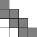
For sufficiently regular functions and over the mesh and , piecewise polynomial approximations , satisfying (7) can be found by appropriate interpolation and choosing the mesh size small enough. Without further structural assumptions on the data, it seems natural to use uniform grids , which can be obtained, e.g., by uniform refinement of some reference grid. In Figure 1, we depict the resulting uniform partitions for approximation of the kernel function .


The evaluation of defined by (6) can be split into two contributions
| (11) |
with corresponding to the integrals over the farfield cells and over the nearfield cells, which are depicted in white and gray in Figure 1, respectively. As discussed in the following subsection, the numerical treatment of these contributions differs slightly.
2.3 Practical realisation
From equation (6) and the choice of and , one can see that is a piecewise polynomial of degree over the grid . It is often convenient to replace by a piecewise polynomial with the same degree as the data. For this purpose, we simply choose a set of distinct points , , and define by collocation
| (12) |
on every time interval , with collocation points , . Now let , , denote the Lagrangian basis of with respect to the interpolation points , i.e.,
| (13) |
Then as a consequence of the uniformity of the mesh , one may deduce that
| (14) |
i.e., the basis is invariant under translation, which will become an important ingredient for our algorithm below. The approximate data and the discrete solution can now be expanded as
| (15) |
In a similar manner, the approximate kernel function can be expanded with respect to a set of bases for the spaces , which leads to
| (16) |
We will again assume translation invariance of this second basis, i.e.,
| (17) |
Note that we allow for different polynomial degrees in the approximations , and , and hence two different sets of basis functions are required. Evaluating (6) at time and utilizing (12), we obtain
| (18) |
where we used the splitting of the integration domain into subintervals of the mesh and an additional separation of farfield and nearfield contributions; see Figure 1. By inserting the basis representations (15) and (16) for , , and , the integrals in the farfield contribution can be expressed as
| (19) |
For convenience of presentation, let us introduce the short-hand notations
| (20) |
and note that the corresponding matrices and are independent of the time steps , , due to the translation invariance conditions (14) and (17). The result vector containing entries from (18) can then be expressed as
| (21) |
with farfield contribution given by
| (22) |
where is the matrix containing the entries . Further introducing the symbols , this may be stated equivalently as . In a similar manner, we may represent the nearfield contribution by
| (23) |
with appropriate nearfield matrices , .
We denote by , the global vectors that are obtained by stacking the element contributions , together. The computation of can then be written as matrix-vector product with block-matrix consisting of blocks as defined above. A possible block-based implementation of this matrix-vector product can be realized as follows.
Remark 2
At first sight, this algorithm may seem more complicated than actually required. In fact, after generating the matrix blocks , the th component of the result vector could also be computed as . The above version, however, is closer to the algorithm developed in the next section. Moreover, it is evolutionary, i.e., the entries of the vector are computed one after another, and oblivious in the sense that only the blocks and are needed for the computation of . Note, however, that all auxiliary values , are required to compute the block and therefore have to be kept in memory. This will be substantially improved in Section 3.2.
2.4 Computational complexity
As indicated above, the computation of according to (18) can be phrased in algebraic form as a matrix-vector product
| (24) |
with and denoting the coefficient vectors for and , and a lower block triangular matrix . Note that the pattern of the matrix is structurally the same as that of the tensor-product grid underlying the approximation of the kernel function ; see Figure 1, with each cell corresponding to a block of size . Thus, the the computation of will in general require operations and memory to store the matrix . In addition, we require active memory to store two values of and the history of .
3 A fast and oblivious algorithm
The aim of this section is to introduce a novel algorithm which allows for a simultaneous compression of the matrix used for the evaluation of (24) and the history of the data stored in the vectors , . The underlying approximation is that of -matrix compression techniques Bor2010 ; Hac2015 . We first collect some results about these hierarchical approximations and then state and analyze our algorithm.
3.1 Multilevel partitioning
For ease of presentation we will assume that the number of time steps is given as with and define . Now let and introduce a hierarchy of nested partitions into subintervals
of length by recursive coarsening of the intervals; see Figure 2 for a sketch.

From the hierarchic construction, one can immediately see that
| (25) |
where denotes the smallest integer larger or equal to as usual.
In a similar spirit to Bor2010 ; FD2009 ; GR1987 ; Hac2015 , we next introduce a multilevel partitioning of the support of the kernel leading to adaptive hierarchical meshes
| (26) |
Note that every element of is square and thus corresponds to one element of a, possibly coarser, uniform mesh . Moreover, any element in is the union of elements of the underlying uniform mesh and can be constructed by recursive agglomeration or coarsening.
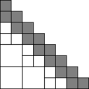
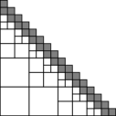
As illustrated in Figure 3, the hierarchic adaptive mesh can again be split into nearfield elements adjacent to the diagonal and the remaining far field elements. Let us remark that the resulting partitioning and its splitting coincide with most of the classical partitioning strategies developed in the context of panel clustering and - and -matrices, see Hac2015 and the references therein.
3.2 Adaptive data sparse approximation
Let be the space of piecewise polynomials of degree in each variable over the mesh . Since the adaptive hierarchical mesh is obtained by coarsening of the underlying uniform grid , we certainly have
Instead of a uniform approximation as used in Section 2.2, we now consider adaptive approximations for the evaluation of (6) or (18).
Remark 3
Let us assume for the moment that the kernel in (2) is asymptotically smooth, i.e., there exist constants , such that
| (27) |
for all , and all . As shown in Bor2010 ; Hac2015 , adaptive approximations can be constructed for asymptotically smooth kernels, which converge exponentially in in the farfield. As a consequence, the same level of accuracy required in Lemma 1 can be achieved by adaptive approximations with much less degrees of freedom than by uniform approximations.
Remark 4
It is not difficult to see that while . The adaptive hierarchical approximation thus is data-sparse and leads to substantial savings in the memory required for storing the kernel approximation or its matrix respresentation (24); compare to Lemma 3 at the end of this section. In addition, an appropriate reorganisation of the operations required for the matrix-vector product (24) leads to a substantial reduction of computational complexity. Moreover, the fast evaluation also induces an automatic compression of the history of the data.
3.3 Multilevel hierarchical basis
In order to obtain algorithms for the matrix-vector-multiplication (3) of quasi-optimal complexity, we require the following second fundamental ingredient. Based on the multilevel hierarchy of time intervals and the translation invariance of the basis functions , we define a multilevel basis
| (28) |
for the spaces , appearing in the far field blocks of the approximation . Let us note that by translation invariance, the coefficients and are independent of and .
For each of the elements of the adaptive partition , we expand the kernel function as
| (29) |
For the computation of the farfield contributions in (18), we can further split the integration domain into
| (30) |
with , , and . Here denotes the th digit from behind of the binary representation of obtained by Matlab’s dec2bin function. This partitioning of the integration domain exactly corresponds to the cells of a corresponding row in the adaptive mesh ; see Figure 4 for an illustration. More precisely, describes the number of different coarsening levels involved in the th row, corresponds to the number of intervals on each level, and yields the indices of these intervals on level .

By inserting the splitting of the integration domain in (30) into equation (18), we obtain
We can now further insert the expansions (29) for the kernel into the farfield integrals over to see that
with auxiliary values
By the recursive definition of , the latter expression can be rewritten as
for complemented with as defined on the uniform grid in Section 2.2. Evaluation of the recursion (28) at time further yields
such that we may define intermediate values
The result of the integral (18) then is finally obtained by
with nearfield contributions and projections as given in (20) and (22). The above derivations can be summarized as follows.
Remark 5
The Matlab function returns the integer generated by a bit-wise xor comparison of the binary representation of and in complexity. This allows to determine in complexity in each step and is required for achieving a theoretical runtime of . In actual implementations one may just set , without any notable difference in computation times. Further note that only one value and two values of are required for each level . Moreover, at most two values of are required at any timestep. The required buffers are denoted by , , and , , . The complexity of the overall algorithm is analyzed in detail in the next section.
Remark 6
Readers familiar with -matrices or the fast multipole method may notice that our algorithm is similar to the corresponding matrix-vector multiplications but with rearranged computations. In each time step, the algorithm checks for changes in the matrix partitioning structure compared to the previous time step. Then, starting from the coarsest level, an upward pass of one level is executed for all coarsened intervals of the farfield by applying the transfer or multipole-to-multipole matrices. Entities from the coarsened intervals are overwritten. Thereafter the farfield interactions are computed by applying the kernel or multipole-to-local matrices corresponding to the changed intervals and directly including the contributions of the next coarser level with a downward pass by appling transfer or local-to-local matrices. Finally, the nearfield contributions are applied.
3.4 Complexity estimates
In the following, we consider Algorithm 2 for the evaluation of (18) with approximate kernel and data , and with denoting the number of time intervals in . The assertions of the following two lemmas are well-known, see e.g. Bor2010 , but their reasoning is simple and illustrative such that we repeat it for the convenience of the reader.
Lemma 2
Algorithm 2 can be executed in operations.
Proof
The algorithm rearranges the operations of a standard -matrix-vector multiplication without adding any significant operations. We therefore simply estimate the complexity of the corresponding -matrix-vector multiplication. Let us first remark that the computation of in line 21 requires operations in each time step. Second, on a given level , we have to perform applications of and in total for obtaining the from the ones on level , see line 7. Similarly, applications of in line 16 are in total required on level for the computation of the and multiplications by need to be performed in lines 12 and 14. Finally, values of and need to be computed in line 9 and line 22. Summing up yields
and since Young’s inequality yields the assertion. ∎
Lemma 3
The -matrix representation of the adaptive hierarchic approximation can be stored in memory. If the kernel is of convolution type (4), then the memory cost reduces to .
Proof
The proof for the adaptive approximation is similar to the previous lemma, with the -related term arising from the nearfield and the -related term from the farfield. For a kernel of convolution type, the hierarchical approximation provides a block Toeplitz structure, such that we only have to store coefficient matrices per level for the farfield and coefficient matrices for the nearfield. ∎
Let us finally also remark on the additional memory required during execution.
Lemma 4
The active memory required for storing the data history required for Algorithm 2 is bounded by .
Proof
We require vectors of length for the nearfield and at most two vectors of length on levels for the farfield contributions. ∎
3.5 Summary
In this section, we discussed the adaptive hierarchical data sparse approximation for the dense system matrix in (3) stemming from a uniform polynomial-based discretization of the Volterra-integral operators (2). This approximation amounts to an -matrix compression of the system matrix, leading to storage complexity for general and storage complexity for convolution kernels. Using a multilevel basis representation on the hierarchy of the time intervals, we formulated a fast and oblivious evolutionary algorithm for the numerical evaluation of Volterra integrals (2). The overall complexity for computing the matrix-vector product in (3) is and only memory is required to store the compressed history of the data. The algorithm is executed in an oblivious and evolutionary manner and can therefore be generalized immediately to integro-differential equations of the form (1). Moreover, knowledge of the number of time steps is not required prior to execution.
4 Approximation of convolution operators
While our algorithm for the fast evaluation of Volterra integral operators is based on a time domain approximation, in many interesting applications, see Lub2004 for examples and references, the kernel function in (5) is of convolution type
| (31) |
and only accessible indirectly via its Laplace transform, i.e., the transfer function
Let us note that, at least formally, the evaluation of the kernel function in the time domain can be achieved by the inverse Laplace transform
| (32) |
where is an appropriate contour connecting with ; see ABHN2011 for details. To ensure the existence of the inverse Laplace transform, we require that
| is analytic in a sector , , | (33) | ||
| and for some fixed , | (34) |
and tacitly assume that the contour lies within the domain of analyticity of the function . In this section, we show that with some minor modifications, Algorithm 2 and our analysis are applicable also in this setting and we compare our method with the fast and oblivious convolution quadrature of LS2002 ; SLL2006 .
4.1 Approximation and numerical realization
As a first step, we show that the convolution kernel given implicitly by (32) indeed satisfies the assumption (27) on asymptotic smoothness. Thus an accurate adaptive hierarchical approximation as discussed in Section 3 is feasible.
Lemma 5
Proof
It is sufficient to consider the case in (33) and in (34). Otherwise, we simply transform and with for . From (ABHN2011, , Theorem 2.6.1), also see Sov1979 , we deduce that has a holomorphic extension into the sector with as in (33). Thus, the radius of convergence of the Taylor series of around is given by , with independent of . This implies
for some constant . Condition (27) then follows by the chain rule. ∎
For the construction of the adaptive approximation , we can now proceed in complete analogy to (11), i.e., we split the convolution integral
| (35) |
into a farfield and a nearfield contribution. The latter can be computed stably and efficiently with Lubich’s convolution quadrature; see Lub1988 ; Lub1988a for details.
For the farfield contributions, we utilise the adaptive hierarchical approximation discussed in the previous section. If direct access to the kernel is available, Algorithm 2 can be applied directly. If, on the other hand, only the transfer function is accessible, the values of can be computed by fast numerical Laplace inversion; see DW2015 ; LPS2006 ; Tal1979 . Here we follow the approach of LPS2006 ; SLL2006 which is based on hyperbolic contours of the form
| (36) |
with , , and , such that the contour remains in the sector of analyticity (33) of . The discretisation of the contour integral (32) by the trapezoidal rule with uniform step with yields
| (37) |
with . Given we are interested in for and have fixed values for and , suitable parameters and are given by
where is the machine precision and
see LPS2006 ; SLL2006 . In our examples in Section 5 we chose , . For error bounds concerning this approach we refer to LPS2006 ; SLL2006 .
4.2 Comparison with fast and oblivious convolution quadrature
Similar to Algorithm 2, the fast and oblivious convolution quadrature (FOCQ) method of LS2002 ; SLL2006 is also based on a splitting (35) of the convolution integral into nearfield and farfield contributions, and the former can again be computed stably and efficiently with Lubich’s convolution quadrature Lub1988 ; Lub1988a .
A different adaptive hierarchic approximation based on L-shaped cells is now used for the approximation in the farfield; see Figure 5.
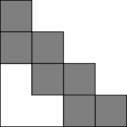


The farfield part of the integration domain for computing the entry is then partitioned into
Choosing an appropriate contour , see (36), and corresponding quadrature points for each farfield cell and using (37) yields an approximation
| (38) | ||||
with and . The values can be computed by numerically solving the ordinary differential equation
| (39) |
with appropriate values and . Thus, the fast and oblivious convolution quadrature provides an approximation of the convolution matrix by solving an auxiliary set of differential equations. In order to obtain an oblivious algorithm it is crucial that the solution of each differential equation is updated in each time step, i.e., the compressed convolution matrix must be evaluated from left to right; see LS2002 ; SLL2006 for details.
The connection to our approach is revealed upon noticing that the compression approach underlying the fast and oblivious convolution quadrature actually implements a low-rank approximation in each of the farfields L-shaped blocks, i.e.,
The corresponding farfield approximation (38) thus effectively reads
which can be understood as a low-rank matrix-vector product realized implicitly by the numerical solution of a differential equation. Since the partitioning depicted in Figure 5 can easily be refined to an adaptive partitioning as in Figure 3, the fast and oblivious convolution quadrature can be interpreted as a particular case of an -matrix approximation with a particular realisation of the -matrix-vector product. The memory cost and complexity of the algorithm can then be immediately deduced from -matrix literature Bor2010 ; Hac2015 .
As mentioned in the introduction, the algorithm proposed in Section 3.2, with the modifications discussed above, is based on an -matrix approximation and leads to a better complexity of . It is also clear that the number of quadrature points for the numerical Laplace inversion determines the ranks of the far-field approximations for the -matrix approximations, which allows for an improved understanding of the approximation error in terms of the approximation order.
5 Numerical examples
In the following we present a series of numerical examples to illustrate and verify the capabilities of our novel algorithms. The experiments are performed in Matlab, in which we implemented our new algorithm as well as a version of the fast-and-oblivious convolution-quadrature algorithm of LPS2006 ; LS2002 for reference. Although our new algorithm performed considerably faster in all of the following examples, we do not present a detailed comparison.
In accordance with the - and -literature, we require the farfield cells in our implementation to be at least times larger than the nearfield cells. This simply means that the cells in Figure 3 represent blocks of fine-grid cells. Following (Bru2004, , Chapter 2), we choose Radau-IIA collocation methods of stage , for the discretization of the Volterra integral operators, which is exactly the scheme used for the approximation as outlined in Section 2.2 and the beginning of Section 2.3. This fixes the approximation spaces for the solution and the data . The error of this discretization scheme is given by
| (40) |
for smooth data and kernel ; see (Bru2004, , Chapter 2) for details. For convolution kernels , we utilize Lubich’s convolution quadrature Lub1988 ; Lub1988a in the near field and the same strategy as above in the farfield. Again, the Radau-IIA method is used as the underlying integration scheme. discretization scheme in the near field is that of. This allows to estimate the approximation error by
| (41) |
for transfer functions satisfying (33)–(34) and data ; see LO1993 for details. The parameter is related to the singularity of the kernel at .
5.1 Variation of constants formula
The first example is dedicated to the solution of the differential equation
| (42) | ||||
| (43) |
By the variation of constants formula, the solution can be expressed as
| (44) |
Let us note that the integral kernel satisfies the asymptotic smoothness assumption (27), but is not of convolution type . To obtain a reference solution, we solve (42)–(43) numerically with a 3-stage Radau-IIA method and with time steps. For the numerical solution of (44), we then employ Algorithm 2 with polynomial degree for the kernel approximation and various degrees for the approximation of the data and the solution .
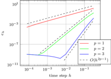
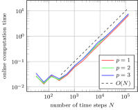
5.2 Nonlinear Volterra integral equation
We continue with a second test example taken from SLL2006 , in which we consider the nonlinear Volterra integral equation
In this example, the convolution kernel is of convolution type, with Laplace transform given by . The evaluation of the integral kernel is realized via numerical inverse Laplace transforms with quadrature points and the kernel is approximated by piecewise polynomials of degree in the farfield; see Section 4. Since the data here depend on , a nonlinear equation must be solved for each time step, for which we employ a Newton method up to a tolerance of . As a reference solution for computing the errors, we here simply take the numerical solution computed on a finer grid.
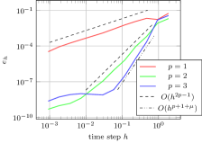
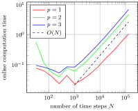
The results of Figure 7 again clearly show the predicted convergence rates up to the point where numerical noise begins to dominate, see (41) with , and the linear complexity of Algorithm 2.
5.3 Fractional diffusion with transparent boundary conditions
As a last example, which is taken from CLP2006 ; SLL2006 , we consider the one-dimensional fractional diffusion equation
with , for and . For the computations, we restrict the spatial domain to , assume that and have support in , and impose transparent boundary conditions on which read
we refer to Hag1999 ; SLL2006 for further details on the model. The Laplace transform of the convolution kernel is here given by .
For the spatial discretisation we employ a finite difference scheme on an equidistant mesh , , and use second-order finite differences within the domain and central differences to approximate the normal derivative on the boundary; see CLP2006 ; SLL2006 . For the time discretisation we employ the frequency domain version of our algorithm with quadrature points for the inverse Laplace transform and polynomial degree for the farfield interpolation. We note that two different convolution quadratures are required, one for the fractional derivative in involving and one for the fractional derivative of the boundary values, involving .
For the space discretisation we consider a fixed mesh with which is fine enough to let the error of the time discretisation dominate. As a reference solution we take the method with order on a finer mesh.
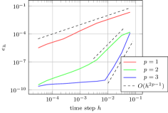
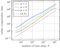
Let us note that due to the lack of temporal smoothness of the solution at , we cannot expect the full order of convergence as predicted by (41); we refer to (CLP2006, , Section 1) for further discussion. In Figure 8, we however still observe a very good approximation in the pre-asymptotic phase and a substantial improvement in accuracy until the numerical noise level is reached when using higher approximation order . As predicted by the theory, the computation times again increase linearly in the number of time steps. In the numerical tests, identical results were obtained for direct evaluation of and evaluation of the kernel via inverse Laplace transforms, which indicates that the main approximation error comes from the adaptive hierarchical approximation.
Acknowledgement
The authors would like to thank the first reviewer for an exceptionally careful reading and valuable comments and remarks.
Funding
Support by the German Science Foundation (DFG) via TRR 146 (project C3), TRR 154 (project C04), and SPP 2256 (project Eg-331/2-1) is gratefully acknowledged.
References
- [1] B. Alpert, L. Greengard, and T. Hagstrom. Rapid evaluation of nonreflecting boundary kernels for time-domain wave propagation. SIAM Journal on Numerical Analysis, 37(4):1138–1164, 2000.
- [2] S. Amari. Dynamics of pattern formation in lateral-inhibition type neural fields. Biological Cybernetics, 27(2):77–87, 1977.
- [3] W. Arendt, C.J.K. Batty, M. Hieber, and F. Neubrander. Vector-Valued Laplace Transforms and Cauchy Problems. Springer Basel, Basel, 2011.
- [4] D. Baffet and J.S. Hesthaven. A Kernel Compression Scheme for Fractional Differential Equations. SIAM Journal on Numerical Analysis, 55(2):496–520, January 2017.
- [5] S. Börm. Efficient Numerical Methods for Non-Local Operators, volume 14 of EMS Tracts in Mathematics. European Mathematical Society (EMS), Zürich, 2010.
- [6] A. Brandt and A.A. Lubrecht. Multilevel matrix multiplication and fast solution of integral equations. Journal of Computational Physics, 90(2):348–370, October 1990.
- [7] H. Brunner. Collocation Methods for Volterra Integral and Related Functional Differential Equations. Number 15 in Cambridge Monographs on Applied and Computational Mathematics. Cambridge University Press, Cambridge, UK ; New York, 2004.
- [8] H. Brunner. Volterra Integral Equations: An Introduction to Theory and Applications. Cambridge University Press, Cambridge, 2017.
- [9] E. Cuesta, C. Lubich, and C. Palencia. Convolution quadrature time discretization of fractional diffusion-wave equations. Mathematics of Computation, 75(254):673–697, January 2006.
- [10] W. Dahmen, S. Prössdorf, and R. Schneider. Wavelet approximation methods for pseudodifferential equations II: Matrix compression and fast solution. Advances in Computational Mathematics, 1(3):259–335, October 1993.
- [11] B. Dingfelder and J.A.C. Weideman. An improved Talbot method for numerical Laplace transform inversion. Numerical Algorithms, 68(1):167–183, January 2015.
- [12] J. Dölz, H. Egger, and V. Shashkov. A convolution quadrature method for Maxwell’s equations in dispersive media, 2020.
- [13] H. Egger, K. Schmidt, and V. Shashkov. Multistep and Runge–Kutta convolution quadrature methods for coupled dynamical systems. Journal of Computational and Applied Mathematics, page 112618, January 2020.
- [14] W. Fong and E. Darve. The black-box fast multipole method. Journal of Computational Physics, 228(23):8712–8725, December 2009.
- [15] K. Giebermann. Multilevel approximation of boundary integral operators. Computing, 67(3):183–207, 2001.
- [16] L. Greengard and V. Rokhlin. A fast algorithm for particle simulations. Journal of Computational Physics, 73(2):325–348, 1987.
- [17] W. Hackbusch. A sparse matrix arithmetic based on -matrices part I: Introduction to -matrices. Computing, 62(2):89–108, 1999.
- [18] W. Hackbusch. Hierarchical Matrices: Algorithms and Analysis. Springer, Heidelberg, 2015.
- [19] W. Hackbusch and Z.P. Nowak. On the fast matrix multiplication in the boundary element method by panel clustering. Numerische Mathematik, 54(4):463–491, July 1989.
- [20] T. Hagstrom. Radiation boundary conditions for the numerical simulation of waves. Acta Numerica, 8:47–106, January 1999.
- [21] E. Hairer, Ch. Lubich, and M. Schlichte. Fast Numerical Solution of Nonlinear Volterra Convolution Equations. SIAM Journal on Scientific and Statistical Computing, 6(3):532–541, July 1985.
- [22] S. Jiang and L. Greengard. Fast evaluation of nonreflecting boundary conditions for the Schrödinger equation in one dimension. Computers & Mathematics with Applications, 47(6-7):955–966, March 2004.
- [23] S. Jiang and L. Greengard. Efficient representation of nonreflecting boundary conditions for the time-dependent Schrödinger equation in two dimensions. Communications on Pure and Applied Mathematics, 61(2):261–288, February 2008.
- [24] S. Kapur, D.E. Long, and J. Roychowdhury. Efficient time-domain simulation of frequency-dependent elements. In Proceedings of International Conference on Computer Aided Design, pages 569–573, San Jose, CA, USA, 1996. IEEE Comput. Soc. Press.
- [25] J. Kaye and D. Golež. Low rank compression in the numerical solution of the nonequilibrium Dyson equation. SciPost Physics, 10(4):091, 2021.
- [26] M. López-Fernández, C. Palencia, and A. Schädle. A Spectral Order Method for Inverting Sectorial Laplace Transforms. SIAM Journal on Numerical Analysis, 44(3):1332–1350, January 2006.
- [27] Ch. Lubich. Convolution quadrature and discretized operational calculus. I. Numerische Mathematik, 52(2):129–145, January 1988.
- [28] Ch. Lubich. Convolution quadrature and discretized operational calculus. II. Numerische Mathematik, 52(4):413–425, July 1988.
- [29] Ch. Lubich. Convolution Quadrature Revisited. BIT Numerical Mathematics, 44(3):503–514, August 2004.
- [30] Ch. Lubich and A. Ostermann. Runge-Kutta methods for parabolic equations and convolution quadrature. Mathematics of Computation, 60(201):105–105, January 1993.
- [31] Ch. Lubich and A. Schädle. Fast Convolution for Nonreflecting Boundary Conditions. SIAM Journal on Scientific Computing, 24(1):161–182, January 2002.
- [32] R. Metzler and J. Klafter. The random walk’s guide to anomalous diffusion: A fractional dynamics approach. Physics Reports, 339(1):1–77, December 2000.
- [33] V. Rokhlin. Rapid solution of integral equations of classical potential theory. Journal of Computational Physics, 60(2):187–207, September 1985.
- [34] F.-J. Sayas. Retarded Potentials and Time Domain Boundary Integral Equations, volume 50 of Springer Series in Computational Mathematics. Springer International Publishing, Cham, 2016.
- [35] A. Schädle, M. López-Fernández, and Ch. Lubich. Fast and Oblivious Convolution Quadrature. SIAM Journal on Scientific Computing, 28(2):421–438, January 2006.
- [36] M. Sova. The Laplace transform of analytic vector-valued functions (complex conditions). Časopis pro pěstování matematiky, 104(3):267–280, 1979.
- [37] A. Talbot. The Accurate Numerical Inversion of Laplace Transforms. IMA Journal of Applied Mathematics, 23(1):97–120, 1979.