Co-matching: Combating Noisy Labels by Augmentation Anchoring
Abstract
Deep learning with noisy labels is challenging as deep neural networks have the high capacity to memorize the noisy labels. In this paper, we propose a learning algorithm called Co-matching, which balances the consistency and divergence between two networks by augmentation anchoring. Specifically, we have one network generate anchoring label from its prediction on a weakly-augmented image. Meanwhile, we force its peer network, taking the strongly-augmented version of the same image as input, to generate prediction close to the anchoring label. We then update two networks simultaneously by selecting small-loss instances to minimize both unsupervised matching loss (i.e., measure the consistency of the two networks) and supervised classification loss (i.e. measure the classification performance). Besides, the unsupervised matching loss makes our method not heavily rely on noisy labels, which prevents memorization of noisy labels. Experiments on three benchmark datasets demonstrate that Co-matching achieves results comparable to the state-of-the-art methods.
1 Introduction
Deep Neural Networks (DNNs) have shown remarkable performance in a variety of applications [19, 24, 38]. However, the superior performance comes with the cost of requiring a correctly annotated dataset, which is extremely time-consuming and expensive to obtain in most real-world scenarios. Alternatively, we may obtain the training data with annotations efficiently and inexpensively through either online key search engine [22] or crowdsourcing [49], but noisy labels are likely to be introduced consequently. Previous studies [2, 50] demonstrate that fully memorizing noisy labels affects accuracy of DNNs significantly, hence it is desirable to develop effective algorithms for learning with noisy labels.
To handle noisy labels, most approaches focus on estimating the noise transition matrix [12, 30, 37, 44] or correcting the label according to model prediction [26, 31, 39, 46]. However, it is challenging to estimate the noise transition matrix especially when the number of classes is large. Another promising direction of study proposes to train two networks on small-loss instances [7, 14, 43, 47], wherein Decoupling [27] and Co-teaching+ [47] introduce the “Disagreement” strategy to keep the two networks diverged to achieve better ensemble effects. However, the instances selected by “Disagreement” strategy are not guaranteed to have correct labels [14, 43], resulting in only a small portion of clean instances being utilized in the training process. Co-teaching [14] and JoCoR [43] aim to reduce the divergence between two different networks so that the number of clean labels utilized in each mini-batch increases. In the beginning, two networks with different learning abilities filter out different types of error. However, with the increase of training epochs, two networks gradually converge to a consensus and even make the wrong predictions consistently.
To address the above concerns, it is essential to keep a balance between divergence and consistency of the two networks. Inspired by augmentation anchoring [5, 35] from semi-supervised learning, we propose a method using weak (e.g. using only crop-and-flip) and strong (e.g. using RandAugment [9]) augmentations for two networks respectively to address the consensus issue. Specifically, one network produces the anchoring labels based on weakly-augmented images. The anchoring labels are used as targets when the peer network is fed the strongly-augmented version of the same images. Their difference is captured by an unsupervised matching loss. Stronger augmentation results in disparate predictions, which guarantees the divergence between two networks, unless they have learned robust generalization ability. As early-learning phenomenon shows that the networks fit training data with clean labels before memorizing the samples with noisy labels [2]. Co-matching trains two networks with a loss calculated by interpolating between two loss terms: 1) A supervised classification loss encourages learning from clean labels during the early-learning phase. 2) An unsupervised matching loss limits the divergence of two networks and prevents memorization of noisy labels after the early-learning phase. In each training step, we use the small-loss trick to select the most likely clean samples, thus ensuring the error flow from the biased selection would not be accumulated.
To show that Co-matching improves the robustness of deep learning on noisy labels, we conduct extensive experiments on both synthetic and real-world noisy datasets, including CIFAR-10, CIFAR-100 and Clothing1M datasets. Experiments show that Co-matching significantly advances state-of-the-art results with different types and levels of label noise. Besides, we study the impact of data augmentation and provide ablation study to examine the effect of different components in Co-matching.
2 Related work
2.1 Learning with Noisy labels
Curriculum learning. Inspired from human cognition, Curriculum learning (CL) [4] proposes to start from easy samples and go through harder samples to improve convergence and generalization. In the noisy label scenario, easy (hard) concepts are associated with clean (noisy) samples. Based on CL, [32] leverages an additional validation set to adaptively assign weights to noisy samples for less loss contribution in every iteration.
Small-loss selection. Another set of emerging methods aim to select the clean labels out of the noisy ones to guide the training. Previous work [2] empirically demonstrates the early-learning phenomenon that DNNs tend to learn clean labels before memorizing noisy labels during training, which justifies that instances with small-loss values are more likely to be clean instances. Based on this observation, [25] proposes a curriculum loss that chooses samples with small-loss values for loss calculation. MentorNet [17] pre-trains a mentor network for selecting small-loss instances to guide the training of the student network. Nevertheless, similar to Self-learning approach, MentorNet inherits the same inferiority of accumulated error caused by the sample-selection bias.
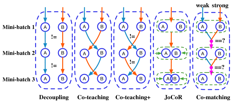
Two classifiers with Disagreement and Agreement. Inspired by Co-training [6], Co-teaching [14] symmetrically trains two networks by selecting small-loss instances in a mini-batch for updating the parameters. These two networks could filter different types of errors brought by noisy labels since they have different learning abilities. When the error from noisy data flows into the peer network, it will attenuate this error due to its robustness [14]. However, two networks converge to a consensus gradually with the increase of epochs. To tackle this issue, Decoupling [27] and Co-teaching+ [47] introduce the “Update by Disagreement” strategy which conducts updates only on selected instances, where there is a prediction disagreement between two classifiers. Through this, the decision of “when to update” depends on a disagreement between two networks instead of depending on the noisy labels. As a result, it would reduce the dependency on noisy labels as well as keep two networks divergent. However, as noisy labels are spread across the whole space of examples, there may be very few clean labels in the disagreement area. Thus, JoCoR [43] suggests jointly training two networks with the instances that have prediction agreement between two networks. However, the two networks in JoCoR are also prone to converge to a consensus and even make the same wrong predictions when datasets are under high noise ratio. This phenomenon will be explicitly shown in our experiments in the symmetric-80%. We compare all these approaches in Figure 1.
Other methods. Some approaches focus on creating noise-tolerant loss functions [11, 40, 42, 51]. Other methods attempt to adjust the loss [1, 16, 26, 30, 31, 36, 39, 41]. Many approaches [10, 21, 29, 39, 43] have been proposed to combat noisy labels through semi-supervised learning.

2.2 Semi-supervised learning
Semi-supervised learning provides a means of leveraging unlabeled data to improve a model’s performance when only limited labeled data is available. Current methods follow into three classes: pseudo-labeling [28, 34] leverages the idea that we should use the model itself to obtain artificial labels for unlabeled data; consistency regularization [3, 20, 33] forces the model to produce consistent predictions on perturbed versions of the same image; entropy minimization [13] encourages the model’s output distribution to be low entropy (i.e., make “high-confidence” predictions) on unlabeled data. Recent works [5, 35] apply augmentation anchoring to replace the consistency regularization as it shows stronger generalization ability.
3 Method
In this section, we describe the main components of the proposed approach Co-matching, including structure, loss function, parameter update and augmentation. In addition, we discuss the relations between Co-matching and other existing approaches.
3.1 Our algorithm: Co-matching
Notations. Consider the -class classification problem, we have a training set with being the one-hot vector corresponding to . In the noisy label scenario, is of relatively high probability to be wrong. We denote the two deep networks in Co-matching as and with parameters and respectively. and are the softmax probabilities produced by and . For the model inputs, we perform two types of augmentation for each network as part of Co-matching: weak and strong, denoted by and respectively. We will describe the forms of augmentation used for and in section 3.2.
Structure. A diagram of Co-matching is shown in Figure 2. Co-matching trains two networks simultaneously, as two networks have different abilities to filter out different types of error. By doing this, it suppresses the accumulated error in self-training approach [17] with single network.
Loss function. [2, 50] experimentally demonstrate that standard cross-entropy loss easily fits the label noise, as its target distribution heavily depends on noisy labels, resulting in undesirable classification performance. To reduce the dependency on noisy labels, the loss function in Co-matching exclusively consists of two loss terms: a supervised loss for classification task and an unsupervised matching loss for augmentation anchoring. Our total loss on is calculated as follows:
| (1) |
where is a fixed scalar hyperparameter controlling the importance weight of the two loss terms. Since there are correctly labeled information remaining in noisy labels, classification loss is the standard cross-entropy loss on noisy labeled instances.
| (2) | ||||
For an image , we feed two networks with different levels of augmented images and respectively, and stronger augmented image generates disparate prediction compare to the weak one. In this way, Co-matching can always keep two networks diverged throughout the whole training to achieve better ensemble effects. Nonetheless, solely keeping the divergence of two networks will not promote the learning ability to select clean labels by “small-loss” trick, which is the main drawback of Co-teaching+ as we discussed in Section 2.
To ensure that Co-matching selects more clean labels, we maximize consistency of the two networks as it helps the model find a much wider minimum and provides better generalization performance. In Co-matching, we compute an anchoring label for each sample by the prediction of model . To obtain an anchoring label, we first compute the predicted class distribution of model given a weakly-augmented version of the image: and . Then, we use hard pseudo-labeling way to get as the anchoring label.
| (3) |
The use of hard pseudo-labeling has the similar function to entropy maximization [13], where the model’s predictions are encouraged to be low-entropy (i.e., high-confidence). The anchoring label is used as the target for a strongly-augmented version of same image in . We use the standard cross-entropy loss rather than mean squared error or Jensen-Shannon Divergence as it maintains stability and simplifies implementation. Thus, the unsupervised matching loss is
| (4) |
Due to the gradient of cross-entropy loss is
| (5) |
where is the Jacobian matrix of the neural network dimensional encoding for the th input and . Using hard pseudo-labeling helps the model converge faster as it keeps large before the early-learning stage. By minimizing the total loss in (1), the model consistently improves the generalization performance under different levels of label noise. Under low-level label noise (i.e., 20%), supervised loss takes the lead. Co-matching tends to learn from the clean labels by filtering out noisy labels. Besides, Co-matching gets a better ensemble effect due to the divergent of two networks created by feeding different kinds of augmentations. Under high-level label noise (i.e., 80%), unsupervised matching loss takes the lead such that Co-matching inclines to maximize the consistency of the networks to improves the generalization performance without requiring a large number of clean labels.
Parameter update. DNNs learn clean and easy patterns before memorizing noisy labels [2]. Thus, small-loss instances are more likely to be the ones that are correctly labeled [14]. If we train our classifier to only use small-loss instances in each mini-batch data, it would be resistant to noisy labels. Following Co-teaching, we introduce to control the number of small-loss instances selected in each mini-batch. Intuitively, at the beginning of training, we keep more small-loss instances (with large ) in each mini-batch. As DNNs fit noisy labels gradually, we decrease the quickly at the first epochs to prevent networks from over-fitting to the noisy labels. We then conduct small-loss selection as follows:
| (6) |
After obtaining the small-loss instances set in mini-batch , we calculate the average loss in these examples for further back propagation.
| (7) |
Put all these together, our algorithm Co-matching is described in Algorithm 1. It consists of the loss calculation (step 5-7), “small-loss” selection (step 8-9) and parameter update (step 9-10).
3.2 Augmentation in Co-matching
Co-matching leverages two kinds of augmentations: “weak” and “strong”. In our experiments, weak augmentation is a standard crop-and-flip augmentation strategy. As for “strong” augmentation, we adopt RandAugment [9], which is based on AutoAugment [8]. AutoAugment learns an augmentation strategy based on transformations from the Python Imaging Libraries 111https://www.pythonware.com/products/pil/ using reinforcement learning. Given a collection of transformations (e.g., color inversion, contrast adjustment, translation, etc.), RandAugment randomly select transformations for each sample in a mini-batch. We set in our experiments and explore more options in Section 4.3. As originally proposed, RandAugment uses a single fixed global magnitude that controls the severity of all distortions [9]. Instead of optimizing the hyperparameter magnitude by using grid search, we found that sampling a random magnitude from a pre-defined range at each training step (instead of using a fixed global value) works better for learning with noisy labels.
3.3 Comparison to other approaches
We compare Co-matching with other related approaches in Table 1. Specifically, Decoupling applies the “Disagreement” strategy to select instances while other approaches including Co-matching use “small-loss” criterion. Co-teaching cross-updates parameters of networks to reduce the accumulated error flow. Combining the “Disagreement” strategy with Co-teaching, Co-teaching+ achieves excellent performance by keeping two networks diverged. JoCoR updates the networks jointly with “small-loss” instances selected by using “agreement” strategy. As for Co-matching, we also select “small-loss” instances and updates the network jointly. Besides, we keep the two networks diverged by feeding different degrees of augmentation and using augmentation anchoring to limit their divergence to some degree. As we will show in Section 4.4, these components are crucial to Co-matching’s success under high levels of noise.
| Decoupling | Co-teaching | Co-teaching+ | JoCoR | Co-matching | |
|---|---|---|---|---|---|
| small loss | |||||
| cross update | |||||
| joint update | |||||
| divergence | |||||
| augmentation anchoring |
4 Experiments
4.1 Experimental settings
Datasets. We evaluate the efficacy of Co-matching on two benchmarks with simulated label noise, CIFAR-10 and CIFAR-100 [18], and one real-world dataset, Clothing1M [45]. Clothing1M consists of 1 million training images collected from online shopping websites with noisy labels generated from surrounding texts. Its noise level is estimated at 38.5%. CIFAR-10 and CIFAR-100 are initially clean. Following [30, 31], we corrupt these datasets manually by label transition matrix , where given that noisy label is flipped from clean label . The matrix Q has two representative label noise models: (1) Symmetric flipping [40] is generated by uniformly flipping the label to one of the other class label; (2) Asymmetric flipping [30] is a simulation of fine-grained classification with noisy labels in real world, where the labelers are more likely to make mistakes only within very similar classes. More details are described in supplementary materials.
Baselines. We compare Co-matching (Algorithm 1) with Decoupling [27], Co-teaching [14], Co-teaching+ [47] and JoCoR [43], and implement all methods with default parameters by Pytorch. Note that all compared algorithms do not use extra techniques such as mixup, Gaussian mixture model, temperature sharpening and temporal ensembling to improve the performance.
| Noise ratio | Standard | Decoupling | Co-teaching | Co-teaching+ | JoCoR | Co-Matching |
|---|---|---|---|---|---|---|
| Symmetric-20% | 69.57 0.20 | 69.55 0.20 | 78.07 0.24 | 78.66 0.20 | 85.69 0.06 | 89.78 0.13 |
| Symmetric-50% | 42.48 0.35 | 41.44 0.46 | 71.54 0.17 | 57.13 0.46 | 79.32 0.37 | 86.42 0.18 |
| Symmetric-80% | 15.79 0.37 | 15.64 0.42 | 27.71 4.39 | 24.13 5.54 | 25.97 3.11 | 55.42 1.68 |
| Asymmetric-40% | 69.36 0.23 | 69.46 0.08 | 73.75 0.34 | 69.03 0.30 | 76.38 0.32 | 81.00 0.46 |
Network Structure. For CIFAR-10 and CIFAR-100, we use a 7-layer network architecture follows [43]. The detail information can be found in supplementary material. As for Clothing1M, we use ResNet18 [15] with ImageNet pretrained weights.
Optimizer. For CIFAR-10 and CIFAR-100, Adam optimizer (momentum=0.9) is used with an initial learning rate of 0.001, and the batch size is set to 128. We run 200 epochs in total and linearly decay learning rate to zero from 80 to 200 epochs. For Clothing1M, we also use Adam optimizer (momentum=0.9) and set batch size to 64. We run 20 epochs in total and set learning rate to , and for 5, 5 and 10 epochs respectively.
Initialization. Following [14, 43, 47], we assume the noise rate is known. We set ratio of the small-loss samples , where and for all datasets. If is not known in advance, can be inferred using validation sets [23, 48]. We find that in extremely noisy case (i.e., 80%), selecting more small-loss instances in Co-matching achieves better generalization performance. For in our loss function (1), we search it in [0.05,0.10,,0.95] with a clean validation set for best performance. When validation set is also with noisy labels, we apply the small-loss selection to choose a clean subset for validation. More information about hyperparameter sensitivity analysis can be found in supplementary materials.
| Noise ratio | Standard | Decoupling | Co-teaching | Co-teaching+ | JoCoR | Co-Matching |
|---|---|---|---|---|---|---|
| Symmetric-20% | 35.46 0.25 | 33.21 0.22 | 43.71 0.20 | 49.15 0.24 | 52.43 0.20 | 59.76 0.27 |
| Symmetric-50% | 16.87 0.13 | 15.03 0.33 | 34.30 0.39 | 39.08 0.73 | 42.73 0.96 | 52.52 0.48 |
| Symmetric-80% | 4.08 0.21 | 3.80 0.01 | 14.95 0.15 | 15.00 0.42 | 14.41 0.60 | 33.50 0.74 |
| Asymmetric-40% | 27.23 0.45 | 26.25 0.27 | 28.27 0.22 | 30.45 0.15 | 31.52 0.31 | 37.67 0.35 |
Metrics. To measure the performance, we use the test accuracy, i.e., test accuracy = (# of correct predictions) / (# of test dataset). Higher test accuracy means that the algorithm is more robust to the label noise. Following the [14, 43], we also calculate the label precision in each mini-batch, i.e., label precision = (# of clean labels) / (# of all selected labels). Specifically, we sample of small-loss instances in each mini-batch, and then calculate the ratio of clean labels in the small-loss instances. Intuitively, higher label precision means less noisy instances in the mini-batch after sample selection, and the algorithm with higher label precision is also more robust to the label noise [14, 43]. However, we find that the higher label precision is not necessarily lead to higher test accuracy with extreme label noise, we will explain this phenomenon in Section 4.2. All experiments are repeated five times. The error bar for STD in each figure has been highlighted as shade.
4.2 Comparison with the State-of-the-Arts
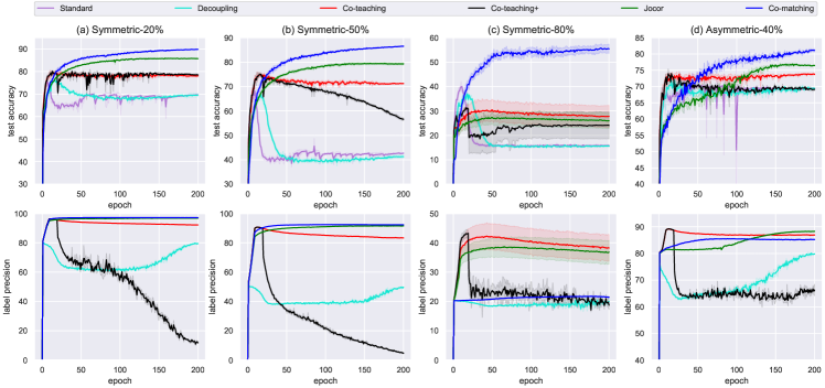
Results on CIFAR-10. Figure 3 shows the test accuracy vs. epochs on CIFAR-10 (top) and the label precision vs. epochs (bottom). With different levels of symmetric and asymmetric label noise, we can clearly see the memorization effect of networks. i.e., test accuracy of Standard first reaches a very high level and then gradually decreases due to the networks overfit to noisy labels. Thus, a robust training approach should alleviate or even stop the decreasing trend in test accuracy. On this point, Co-matching consistently outperforms state-of-the-art methods by a large margin across all noise ratios.
We report the test accuracy of different algorithms in detail in Table 2. In the easiest Symmetric-20% case, all existing approaches except Decoupling perform much better than Standard, which demonstrates their robustness. Compared to the best baseline method JoCoR, Co-matching still achieve more than 4% improvement. When it goes to Symmetric-50% case and Asymmetric 40% case, Co-teaching+ and Decoupling begin to fail a lot while other methods still work fine, especially Co-matching and JoCoR. However, similar to Co-teaching, JoCoR cannot combat with the hardest Symmetric-80% case, where it only achieves 25.97%, which is even worse than Co-teaching (27.71%). In short, JoCoR reduces to Co-teaching in function and suffers the same problem which the two classifiers converge to consensus. We hypothesize the reason is that under high-levels of label noise, there is not enough supervision from clean labels, which leads to the networks making the same wrong predictions even with low confidence. However, Co-matching achieves the best average classification accuracy (55.42%) again.
We also plot label precision vs. epochs at the bottom of Figure 3. Only Decoupling, Co-teaching, Co-teaching+, JoCoR and Co-matching are considered here, as they include sample selection during training. First, we can see Co-matching, JoCoR and Co-teaching can successfully pick clean instances out in Symmetric-20 %, Symmetric-50% and Asymmetric-40% cases. Note that Co-matching not only reaches high label precision in these three cases but also performs better and better with the increase of epochs. Decoupling and Co-teaching+ fail in selecting clean samples, because “Disagreement” strategy does not guarantee to select clean samples, as mentioned in Section 2. However, an interesting phenomenon is that high label precision does not necessarily lead to high test accuracy especially under high-levels of label noise. For example, in Symmetric-80% case, the label precision of Co-matching is much lower than Co-teaching and JoCoR, while the test accuracy is much higher than Co-teaching and JoCoR. More similar cases can be found in results on CIFAR-100.
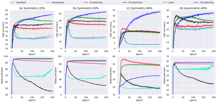
Results on CIFAR-100. The test accuracy and label precision vs. epochs are shown in Figure 4. The test accuracy is shown in Table 3. Similarly, Co-matching still achieves highest test accuracy in all noise cases. In the hardest Symmetric-80% case, Co-teaching, Co-teaching+ and JoCoR tie together, while Co-matching gets much higher test accuracy. When it turns to Asymmetric-40% case, Co-teaching+ and JoCoR achieve the better performance first, while Co-matching gradually surpasses these methods after 75 epochs. Overall, the result shows that Co-matching has better generalization ability than state-of-the-art approaches.
As we discussed before, high label precision does not necessarily lead to high test accuracy. The results in Figure 4 also verify it. As we can see in all four noise rate cases, Co-teaching has much higher label precision than Co-teaching+, while the test accuracy of Co-teaching is lower than Co-teaching+. In the training process, compared to repetitive clean samples, the samples which are near the margins with low confidence and relatively high loss may contribute more towards improving the model’s generalization ability. This explains why Co-matching has low label precision but higher test accuracy in Symmetric-80% case.
Results on Clothing1M. As shown in Table 4, best denotes the epoch where the validation accuracy is optimal, and last denotes the test accuracy at the end of training. Co-matching outperforms the state-of-the-art methods by a large margin on both best and last, e.g., improving the accuracy from 66.95% to 70.71% over Standard, better than best baseline method by 0.92%.
4.3 Composition of data augmentation
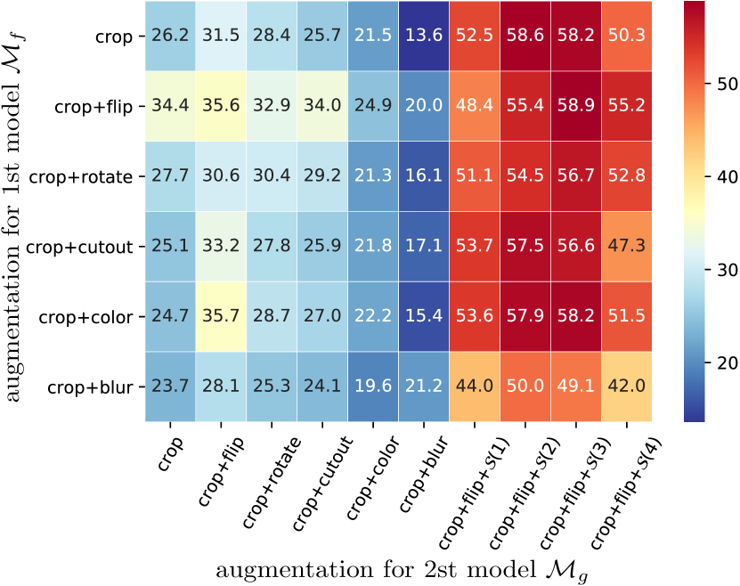
We study the impact of data augmentation systematically by considering several common augmentations. One type of augmentation involves spatial/geometric transformation, such as cropping, flipping, rotation and cutout. The other type of augmentation involves appearance transformation, such as color distortion (e.g. brightness and contrast) and Gaussian blur. Since Clothing1M images are of different sizes, we always use cropping as a base transformation. We explore various “weak” augmentation by combining cropping with other augmentations. As for “strong” augmentation, we use RandAugment [9], which randomly select transformations from a set for each sample in a mini-batch. We denote RandAugment as . In our experiment, Contrast, Equalize, Invert, Rotate, Posterize, Solarize, Color, Brightness, Sharpness, ShearX, ShearY, Cutout, TranslateX, TranslateY, Gaussian Blur.
Figure 5 shows the results under composition of transformations. We observe that using “weak” augmentation for both models does not work much better than simple cropping. However, the performance of Co-matching benefits a lot by using stronger augmentations (e.g. add and ) on second model. We conclude that in extreme label noise case, the unsupervised matching loss requires to use stronger augmentation on model to improve its effect.
4.4 Ablation Study
In this section, we perform an ablation study for analyzing the effect of using two networks and augmentation anchoring in Co-matching. The experiment is conducted on CIFAR-10 with two cases: Symmetric-50% and Symmetric-80%. To verify the effect of using two classifiers, we introduce Standard enhanced by “small-loss” selection (abbreviated as Standard+), Co-teaching and JoCoR to join the comparison. Recall that JoCoR selects instances by the joint loss while Co-teaching uses cross-update approach to reduce the accumulated error [14, 43]. Besides, we simply set in (1) to see the influence of removing augmentation anchoring (abbreviated as Co-matching-).
| Methods | best | last |
|---|---|---|
| Standard | 67.74 | 66.95 |
| Decoupling | 67.71 | 66.78 |
| Co-teaching | 69.05 | 68.99 |
| Co-teaching+ | 67.84 | 67.68 |
| JoCoR | 70.30 | 69.79 |
| Co-matching | 71.03 | 70.71 |
The results of their test accuracy vs. epochs are shown in Figure 6. In Symmetric-50% case, both Co-teaching and Standard+ keep a downward tendency after increasing to the highest point, which indicates they are still prone to memorizing noisy labels even with “small-loss” update. Besides, it proves the effect of using two networks as Co-teaching performs better than Standard+. JoCoR consistently outperforms Co-teaching, which verifies the conclusion in [43] that joint-update is more efficient than cross-update in Co-teaching. However, things start to change in Symmetric-80% case. Co-teaching and Standard+ remain the same trend as these for Symmetric-50% case, but JoCoR performs even worse than Co-teaching and Standard+. Since two networks in JoCoR would be more and more similar due to the effect of Co-regularization, using joint-update works the same as cross-update.
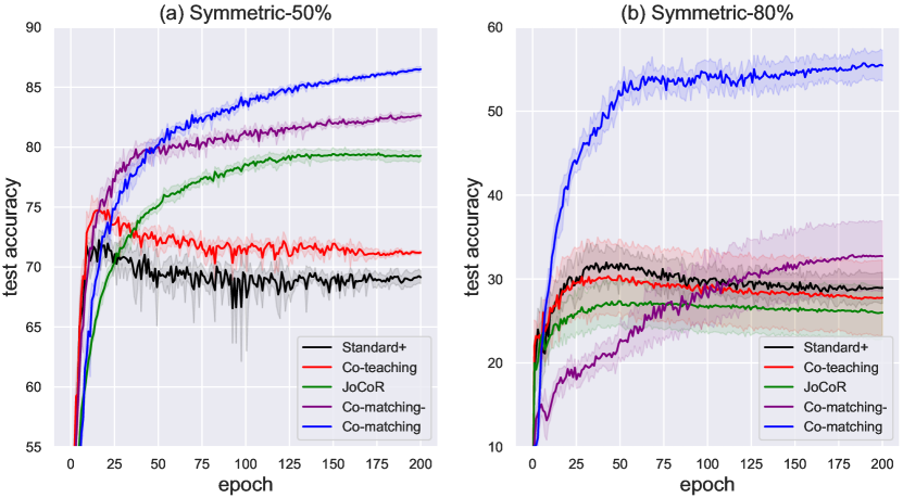
In both cases, Co-matching consistently outperforms Co-matching- and other methods, which validates that augmentation anchoring can strongly prevent neural networks from memorizing noisy labels as it reduces the dependency on noisy labels. In addition, using weak and strong augmentations alone may not promise to improve test accuracy. As we can see in Symmetric-80% case, Co-matching- only slightly outperforms Standard+ after 115 epochs, which also demonstrates that only using the classification loss in (3.1) doesn’t provide a strong supervision since the most noisy labels are incorrect in this case.
5 Conclusion
In this paper, we introduce Co-matching for combating noisy labels. Our method trains two networks simultaneously on “small-loss” samples and achieves robustness to noisy labels through augmentation anchoring between two networks. By balancing the divergence and consistency of two networks, Co-matching obtains state-of-the-art performance on benchmark datasets with simulated and real-world label noise. For future work, we are interested in exploring the effectiveness of Co-matching in other domains.
References
- [1] Eric Arazo, Diego Ortego, Paul Albert, Noel O’Connor, and Kevin Mcguinness. Unsupervised label noise modeling and loss correction. In International Conference on Machine Learning, pages 312–321, 2019.
- [2] Devansh Arpit, Stanislaw K Jastrzebski, Nicolas Ballas, David Krueger, Emmanuel Bengio, Maxinder S Kanwal, Tegan Maharaj, Asja Fischer, Aaron C Courville, Yoshua Bengio, et al. A closer look at memorization in deep networks. In ICML, 2017.
- [3] Philip Bachman, Ouais Alsharif, and Doina Precup. Learning with pseudo-ensembles. In Advances in neural information processing systems, pages 3365–3373, 2014.
- [4] Yoshua Bengio, Jérôme Louradour, Ronan Collobert, and Jason Weston. Curriculum learning. In Proceedings of the 26th annual international conference on machine learning, pages 41–48, 2009.
- [5] David Berthelot, Nicholas Carlini, Ekin D Cubuk, Alex Kurakin, Kihyuk Sohn, Han Zhang, and Colin Raffel. Remixmatch: Semi-supervised learning with distribution alignment and augmentation anchoring. arXiv preprint arXiv:1911.09785, 2019.
- [6] Avrim Blum and Tom Mitchell. Combining labeled and unlabeled data with co-training. In Proceedings of the eleventh annual conference on Computational learning theory, pages 92–100, 1998.
- [7] Pengfei Chen, Ben Ben Liao, Guangyong Chen, and Shengyu Zhang. Understanding and utilizing deep neural networks trained with noisy labels. In International Conference on Machine Learning, pages 1062–1070, 2019.
- [8] Ekin D Cubuk, Barret Zoph, Dandelion Mane, Vijay Vasudevan, and Quoc V Le. Autoaugment: Learning augmentation strategies from data. In Proceedings of the IEEE conference on computer vision and pattern recognition, pages 113–123, 2019.
- [9] Ekin D Cubuk, Barret Zoph, Jonathon Shlens, and Quoc V Le. Randaugment: Practical automated data augmentation with a reduced search space. In Proceedings of the IEEE/CVF Conference on Computer Vision and Pattern Recognition Workshops, pages 702–703, 2020.
- [10] Yifan Ding, Liqiang Wang, Deliang Fan, and Boqing Gong. A semi-supervised two-stage approach to learning from noisy labels. In 2018 IEEE Winter Conference on Applications of Computer Vision (WACV), pages 1215–1224. IEEE, 2018.
- [11] Aritra Ghosh, Himanshu Kumar, and PS Sastry. Robust loss functions under label noise for deep neural networks. In Proceedings of the Thirty-First AAAI Conference on Artificial Intelligence, pages 1919–1925, 2017.
- [12] Jacob Goldberger and Ehud Ben-Reuven. Training deep neural-networks using a noise adaptation layer. 2016.
- [13] Yves Grandvalet and Yoshua Bengio. Semi-supervised learning by entropy minimization. In Advances in neural information processing systems, pages 529–536, 2005.
- [14] Bo Han, Quanming Yao, Xingrui Yu, Gang Niu, Miao Xu, Weihua Hu, Ivor Tsang, and Masashi Sugiyama. Co-teaching: Robust training of deep neural networks with extremely noisy labels. In Advances in neural information processing systems, pages 8527–8537, 2018.
- [15] Kaiming He, Xiangyu Zhang, Shaoqing Ren, and Jian Sun. Deep residual learning for image recognition. In Proceedings of the IEEE conference on computer vision and pattern recognition, pages 770–778, 2016.
- [16] Dan Hendrycks, Mantas Mazeika, Duncan Wilson, and Kevin Gimpel. Using trusted data to train deep networks on labels corrupted by severe noise. In Advances in neural information processing systems, pages 10456–10465, 2018.
- [17] Lu Jiang, Zhengyuan Zhou, Thomas Leung, Li-Jia Li, and Li Fei-Fei. Mentornet: Learning data-driven curriculum for very deep neural networks on corrupted labels. In International Conference on Machine Learning, pages 2304–2313, 2018.
- [18] Alex Krizhevsky, Geoffrey Hinton, et al. Learning multiple layers of features from tiny images. 2009.
- [19] Alex Krizhevsky, Ilya Sutskever, and Geoffrey E Hinton. Imagenet classification with deep convolutional neural networks. In Advances in neural information processing systems, pages 1097–1105, 2012.
- [20] Samuli Laine and Timo Aila. Temporal ensembling for semi-supervised learning. arXiv preprint arXiv:1610.02242, 2016.
- [21] Junnan Li, Richard Socher, and Steven CH Hoi. Dividemix: Learning with noisy labels as semi-supervised learning. In International Conference on Learning Representations, 2020.
- [22] Wen Li, Limin Wang, Wei Li, Eirikur Agustsson, and Luc Van Gool. Webvision database: Visual learning and understanding from web data. arXiv preprint arXiv:1708.02862, 2017.
- [23] Tongliang Liu and Dacheng Tao. Classification with noisy labels by importance reweighting. IEEE Transactions on pattern analysis and machine intelligence, 38(3):447–461, 2015.
- [24] Xihui Liu, Zihao Wang, Jing Shao, Xiaogang Wang, and Hongsheng Li. Improving referring expression grounding with cross-modal attention-guided erasing. In Proceedings of the IEEE Conference on Computer Vision and Pattern Recognition, pages 1950–1959, 2019.
- [25] Yueming Lyu and Ivor W Tsang. Curriculum loss: Robust learning and generalization against label corruption. In International Conference on Learning Representations, 2019.
- [26] Xingjun Ma, Yisen Wang, Michael E Houle, Shuo Zhou, Sarah Erfani, Shutao Xia, Sudanthi Wijewickrema, and James Bailey. Dimensionality-driven learning with noisy labels. In International Conference on Machine Learning, pages 3355–3364, 2018.
- [27] Eran Malach and Shai Shalev-Shwartz. Decoupling” when to update” from” how to update”. In Advances in Neural Information Processing Systems, pages 960–970, 2017.
- [28] Geoffrey J McLachlan. Iterative reclassification procedure for constructing an asymptotically optimal rule of allocation in discriminant analysis. Journal of the American Statistical Association, 70(350):365–369, 1975.
- [29] Tam Nguyen, C Mummadi, T Ngo, L Beggel, and Thomas Brox. Self: learning to filter noisy labels with self-ensembling. In International Conference on Learning Representations (ICLR), 2020.
- [30] Giorgio Patrini, Alessandro Rozza, Aditya Krishna Menon, Richard Nock, and Lizhen Qu. Making deep neural networks robust to label noise: A loss correction approach. In Proceedings of the IEEE Conference on Computer Vision and Pattern Recognition, pages 1944–1952, 2017.
- [31] Scott Reed, Honglak Lee, Dragomir Anguelov, Christian Szegedy, Dumitru Erhan, and Andrew Rabinovich. Training deep neural networks on noisy labels with bootstrapping. arXiv preprint arXiv:1412.6596, 2014.
- [32] Mengye Ren, Wenyuan Zeng, Bin Yang, and Raquel Urtasun. Learning to reweight examples for robust deep learning. In International Conference on Machine Learning, pages 4334–4343, 2018.
- [33] Mehdi Sajjadi, Mehran Javanmardi, and Tolga Tasdizen. Regularization with stochastic transformations and perturbations for deep semi-supervised learning. In Advances in neural information processing systems, pages 1163–1171, 2016.
- [34] H Scudder. Probability of error of some adaptive pattern-recognition machines. IEEE Transactions on Information Theory, 11(3):363–371, 1965.
- [35] Kihyuk Sohn, David Berthelot, Chun-Liang Li, Zizhao Zhang, Nicholas Carlini, Ekin D Cubuk, Alex Kurakin, Han Zhang, and Colin Raffel. Fixmatch: Simplifying semi-supervised learning with consistency and confidence. arXiv preprint arXiv:2001.07685, 2020.
- [36] Hwanjun Song, Minseok Kim, and Jae-Gil Lee. Selfie: Refurbishing unclean samples for robust deep learning. In International Conference on Machine Learning, pages 5907–5915, 2019.
- [37] Sainbayar Sukhbaatar and Rob Fergus. Learning from noisy labels with deep neural networks. arXiv preprint arXiv:1406.2080, 2(3):4, 2014.
- [38] Christian Szegedy, Wei Liu, Yangqing Jia, Pierre Sermanet, Scott Reed, Dragomir Anguelov, Dumitru Erhan, Vincent Vanhoucke, and Andrew Rabinovich. Going deeper with convolutions. In Proceedings of the IEEE conference on computer vision and pattern recognition, pages 1–9, 2015.
- [39] Daiki Tanaka, Daiki Ikami, Toshihiko Yamasaki, and Kiyoharu Aizawa. Joint optimization framework for learning with noisy labels. In Proceedings of the IEEE Conference on Computer Vision and Pattern Recognition, pages 5552–5560, 2018.
- [40] Brendan Van Rooyen, Aditya Menon, and Robert C Williamson. Learning with symmetric label noise: The importance of being unhinged. In Advances in Neural Information Processing Systems, pages 10–18, 2015.
- [41] Yisen Wang, Weiyang Liu, Xingjun Ma, James Bailey, Hongyuan Zha, Le Song, and Shu-Tao Xia. Iterative learning with open-set noisy labels. In Proceedings of the IEEE Conference on Computer Vision and Pattern Recognition, pages 8688–8696, 2018.
- [42] Yisen Wang, Xingjun Ma, Zaiyi Chen, Yuan Luo, Jinfeng Yi, and James Bailey. Symmetric cross entropy for robust learning with noisy labels. In Proceedings of the IEEE International Conference on Computer Vision, pages 322–330, 2019.
- [43] Hongxin Wei, Lei Feng, Xiangyu Chen, and Bo An. Combating noisy labels by agreement: A joint training method with co-regularization. In Proceedings of the IEEE/CVF Conference on Computer Vision and Pattern Recognition, pages 13726–13735, 2020.
- [44] Xiaobo Xia, Tongliang Liu, Nannan Wang, Bo Han, Chen Gong, Gang Niu, and Masashi Sugiyama. Are anchor points really indispensable in label-noise learning? In Advances in Neural Information Processing Systems, pages 6838–6849, 2019.
- [45] Tong Xiao, Tian Xia, Yi Yang, Chang Huang, and Xiaogang Wang. Learning from massive noisy labeled data for image classification. In Proceedings of the IEEE conference on computer vision and pattern recognition, pages 2691–2699, 2015.
- [46] Kun Yi and Jianxin Wu. Probabilistic end-to-end noise correction for learning with noisy labels. In Proceedings of the IEEE Conference on Computer Vision and Pattern Recognition, pages 7017–7025, 2019.
- [47] X Yu, B Han, J Yao, G Niu, IW Tsang, and M Sugiyama. How does disagreement help generalization against label corruption? In 36th International Conference on Machine Learning, ICML 2019, 2019.
- [48] Xiyu Yu, Tongliang Liu, Mingming Gong, Kayhan Batmanghelich, and Dacheng Tao. An efficient and provable approach for mixture proportion estimation using linear independence assumption. In Proceedings of the IEEE Conference on Computer Vision and Pattern Recognition, pages 4480–4489, 2018.
- [49] Xiyu Yu, Tongliang Liu, Mingming Gong, and Dacheng Tao. Learning with biased complementary labels. In Proceedings of the European Conference on Computer Vision (ECCV), pages 68–83, 2018.
- [50] Chiyuan Zhang, Samy Bengio, Moritz Hardt, Benjamin Recht, and Oriol Vinyals. Understanding deep learning requires rethinking generalization. arXiv preprint arXiv:1611.03530, 2016.
- [51] Zhilu Zhang and Mert Sabuncu. Generalized cross entropy loss for training deep neural networks with noisy labels. In Advances in neural information processing systems, pages 8778–8788, 2018.
6 Supplementary Material
6.1 Datasets
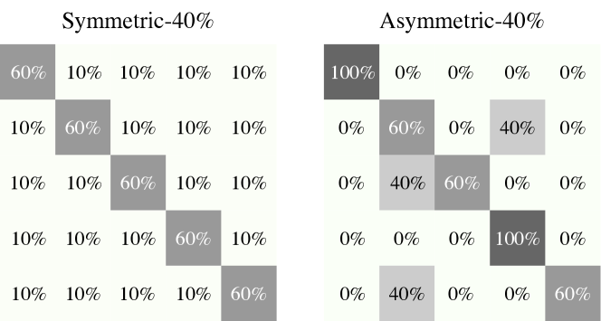
The information of datasets are described in Table 5. For Clothing1M, note that we only use 14k and 10k clean data for validation and test. The 50k clean training data is not required during the training. As for simulating label noise, Figure 7 shows an example of noise transition matrix . Specifically, for CIFAR-10, the asymmetric noisy labels are generated by flipping truck automobile, bird airplane, deer horse and cat dog. For CIFAR-100, the noise flips each class into the next, circularly within super-classes.
| # of train | # of test | # of class | input size | |
|---|---|---|---|---|
| CIFAR-10 | 50,000 | 10,000 | 10 | 32 32 |
| CIFAR-100 | 50,000 | 10,000 | 100 | 32 32 |
| Clothing1M | 1,000,000 | 10,000 | 14 | 224 224 |
6.2 Network Architecture
The network architectures of the CNN model for CIFAR-10 and CIFAR-100 are shown in Table 6.
| CNN on CIFAR-10 & CIFAR-100 |
|---|
| 32 32 RGB Image |
| 3 3, 64 BN, ReLU |
| 3 3, 64 BN, ReLU |
| 2 2 Max-pool |
| 3 3, 128 BN, ReLU |
| 3 3, 128 BN, ReLU |
| 2 2 Max-pool |
| 3 3, 196 BN, ReLU |
| 3 3, 196 BN, ReLU |
| 2 2 Max-pool |
| Dense 256 100 |
6.3 Hyperparameter Sensitivity
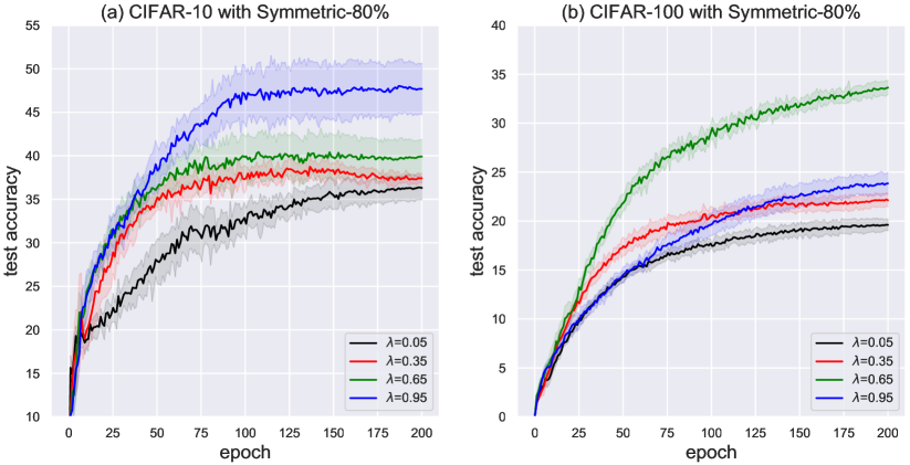
Choice of . To conduct the sensitivity analysis on hyperparameter , we set up the experiments on CIFAR-10 and CIFAR-100 with the hardest Symmetric-80% label noise. Specifically, we compare the in the range of . Recall that controls the importance weights of classification loss and matching loss. A larger means a larger contribution from the matching loss.
Figure 8 shows the test accuracy vs. number of epochs. In the CIFAR-10 Symmetric-80% case, a larger gets a better test accuracy, and achieves the best performance. It verifies the motivation of the loss function in Co-matching: under high-levels of label noise, the model is hard to get enough supervision from noisy labels if we only use the classification loss, more weights on unsupervised loss is required to improve the generalization ability. is the best option in the CIFAR-100 Symmetric-80% case. Because different datasets require different significance of augmentation anchoring, too much weights on unsupervised loss may cause the model hard to converge.
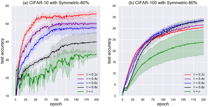
Choice of . The experiments are also conducted on CIFAR-10 and CIFAR-100 with the hardest Symmetric-80% case. Specifically, we compare the in the range of , where is the inferred noise rate that widely used in previous works as we have discussed in the paper. Recall that smaller in increases the number of small-loss instances to be selected. As shown in Figure 9, in CIFAR-10 with Symmetric-80% case, the smaller achieves better and better performance. In CIFAR-100 with Symmetric-80%, is the best option. Overall, under a high-level of label noise, since the augmentation anchoring component requires enough samples for effective training, a proper increase of the selected small-loss instances achieves better generalization ability.
6.4 State-of-the-art methods with the same weak and strong augmentation
We evaluate the state-of-art methods with the same augmentation strategy (i.e. weak and strong for each network respectively) as Co-matching. We set up the experiments on CIFAR-10 with the hardest Symmetric-80% label noise. The weak augmentation is a standard crop-and-flip. The strong augmentation is crop-and-flip and RandAugment with . Figure 10 (a) shows the results. We observe that with the same augmentation strategy, the performance of state-of-the-art methods do not improve a lot. Co-teaching+ even performs worse. Besides, the state-of-the-art methods become more stable as we can see the standard deviation from the mean becomes smaller.
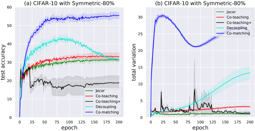
6.5 Divergence of two networks
We compare the divergence of two networks by reporting total variations of softmax output between two networks in Figure 10 (b). We can clearly observe that two networks trained by Co-teaching and Jocor converge to a consensus gradually, while the two networks trained by Co-matching keeps diverged.
6.6 Using hard pseudo-labeling for matching loss
Using hard pseudo-labeling for matching loss helps the model converge. We report the results in Table 7. We find that when the noise reaches to 80%, the Co-matching does not converge with soft pseudo-labeling. That’s the main reason we use hard pseudo-labeling for matching loss.
| Hard pseudo-labeling | Soft pseudo-labeling | |
|---|---|---|
| Symmetric-50% | 86.42 0.18 | 86.43 0.32 |
| Symmetric-80% | 55.42 1.68 | 9.98 0.0 |
6.7 List of Data Augmentations
We use the same sets of image transformation used in RandAugment. For completeness, we describe the all transformation operations for these augmentation strategies in Table 8.
| Transformations | Description | Parameter | Range |
|---|---|---|---|
| Autocontrast | Maximizes the image contrast by setting the darkest (lightest) pixel to black (white). | ||
| Brightness | Adjusts the brightness of the image. returns a black image, returns the original image. | ||
| Color | Adjusts the color balance of the image like in a TV. returns a black& white image, returns the original image. | ||
| Contrast | Controls the contrast of the image. returns a gray image, returns the original image. | ||
| Sharpness | Adjusts the sharpness of the image, where returns a blurred image, and returns the original image. | ||
| Gaussian Blur | Blur the image by Gaussian function | ||
| Solarize | Inverts all pixels above a threshold value of . | ||
| Posterize | Reduces each pixel to bits. | ||
| Equalize | Equalizes the image histogram. | ||
| Identity | Returns the original image. | ||
| Rotate | Rotates the image by degrees. | ||
| ShearX | Shears the image along the horizontal axis with rate . | ||
| ShearY | Shears the image along the vertical axis with rate . | ||
| TranslateX | Translates the image horizontally by ( image width) pixels. | ||
| TranslateY | Translates the image vertically by ( image height) pixels. |