Numerical Characterization of Support Recovery in Sparse Regression with Correlated Design

Abstract

Sparse regression is frequently employed in diverse scientific settings as a feature selection method. A pervasive aspect of scientific data that hampers both feature selection and estimation is the presence of strong correlations between predictive features. These fundamental issues are often not appreciated by practitioners, and jeapordize conclusions drawn from estimated models. On the other hand, theoretical results on sparsity-inducing regularized regression such as the Lasso have largely addressed conditions for selection consistency via asymptotics, and disregard the problem of model selection, whereby regularization parameters are chosen. In this numerical study, we address these issues through exhaustive characterization of the performance of several regression estimators, coupled with a range of model selection strategies. These estimators and selection criteria were examined across correlated regression problems with varying degrees of signal to noise, distribution of the non-zero model coefficients, and model sparsity. Our results reveal a fundamental tradeoff between false positive and false negative control in all regression estimators and model selection criteria examined. Additionally, we are able to numerically explore a transition point modulated by the signal-to-noise ratio and spectral properties of the design covariance matrix at which the selection accuracy of all considered algorithms degrades. Overall, we find that SCAD coupled with BIC or empirical Bayes model selection performs the best feature selection across the regression problems considered.

1 Introduction

In the last several decades, significant research in the mathematics and statistics communities has been directed at the problem of reconstructing a $k$-sparse vector from noisy, linear observations. In its simplest form, one is concerned with inference within the following model:

$$\bm{y}=\bm{X}\beta+\epsilon$$ (1)

with $\bm{y}\in\mathbb{R}^{n},\bm{X}\in\mathbb{R}^{n\times p}$ and $\beta\in\mathbb{R}^{p}$ is a k-sparse vector. The noise is i.i.d, $\epsilon\in\mathbb{R}^{n},\epsilon_{i}\sim\mathcal{N}(0,\sigma^{2})$, and the observational model is Gaussian, $y_{i}\sim\mathcal{N}(\bm{X}_{i}\beta,\epsilon_{i})$. The sparse linear model is employed in diverse scientific fields [satija_spatial_2015, waldmann_evaluation_2013, tibshirani_lasso_1997, steyerberg_towards_2014, wright_sparse_2010]. In real world applications, it is also commonly the case that the design or covariate matrix X is correlated, so that the columns of $\bm{X}$ can not be taken to be i.i.d. In this setting, the correct identification of non-zero elements of $\beta$, which is crucial for scientific interpretability, is especially challenging. Yet, a systematic exploration of the effect of correlations between the covariates on the recoverability of $\beta$ is lacking.

Statistically optimal sparse estimates of $\beta$ within (1) are returned by the solution to the following constrained optimization problem:

$$\min||y-\bm{X}\beta||_{2}^{2}$$ (2)

$$||\beta||_{0}\leq\lambda$$ (3)

Finding the global minima of problem (3) is NP-hard, though recent progress has been made in computationally tractable approaches [zhu_polynomial_2020, bertsimas_best_2016]. The most common approach is to relax the $l_{0}$ regularization. In this work, we focus on the Lasso, Elastic Net, SCAD, MCP [tibshirani_regression_1996, zou_regularization_2005, zhang_nearly_2010, fan_variable_2001], and $\text{UoI}_{\text{Lasso}}$, an inference framework we introduced in [bouchard_union_2017] that combines stability selection and bagging approaches to produce low variance and nearly unbiased estimates. To select the regularization strength or otherwise compare between candidate models returned between these estimators, one must employ a model selection criteria such as cross-validation or BIC. While the literature on sparsity inducing estimators and model selection criteria is vast, studies that consider the interaction of particular choices of estimator and model selection criteria are lacking. In particular, no systematic exploration of the impact of choice of estimator and model selection criteria on the selection accuracy of the resulting procedure when the predictive features exhibit correlations has been carried out. In this work, we address this gap by performing systematic numerical investigations of the selection accuracy performance of several estimators and model selection criteria across a broad range of regression designs, including diverse correlated design matrices. Section 2 summarizes prior theoretical and empirical work on model selection and compressed sensing. We also discus a scalar parameterization of signal strength in correlated sparse regression borrowed from [m._j._wainwright_information-theoretic_2009] that we call $\alpha$. In section 3, we outline the scope of this study and the evaluation criteria used. In Section 4 we present the main results. We characterize the impact of correlated design on the false negative and false positive discovery rates, as well as the magnitude of coefficients likely to be falsely set to zero or false assigned non-zero values. We reveal that estimators and selection methods display a remarkable degree of universality with respect to the correlation strength (quantified by $\alpha$). We also identify the best performing combinations of estimator and selection methods under various signal conditions. Connections to prior theoretical work and concrete recommendations for practitioners are provided in Section 5.

2 Review of Prior Work

The statistical theory of the sparse estimators considered in this work is vast and we do not attempt to review it all here. Our particular focus is on characterizing finite sample selection accuracy, especially in the context of correlated design. The asymptotic oracular selection performance of the SCAD and MCP are well known [fan_variable_2001, zhang_nearly_2010] and require only mild conditions on the design matrix. For the Lasso, one must impose an irrepresentible condition to guarantee asymptotic selection consistency [zhao_model_2006]. The finite sample implications of these differing requirements have not been explored. A series of works have addressed the correlated design problem by devising regularizations that tend to assign correlated covariates similar model coefficients [li_graph-based_2018, figueiredo_ordered_2016, buhlmann_correlated_2013, bogdan_statistical_2013, tibshirani_sparsity_2005, witten_cluster_2014]. In fact, the Elastic Net was the first estimator introduced to exhibit this type of “grouping” effect [zou_regularization_2005]. However, this type of behavior can be undesirable in many real data applications where covariates may be correlated, yet still contribute heterogenously to a response variable of interest.

When the true model generating the data is contained amongst the candidate model supports, the BIC and gMDL have asymptotic guarantees of selection consistency [zhao_model_2006]. Extensions of these results to the high dimensional case are available [kim_consistent_2012], but fall outside the scope of this work. Implicit in these theoretical results is that one can evaluate the penalized likelihoods on all $2^{p}$ candidate model supports [shao_asymptotic_1997]. Practically, one first assembles a much smaller set of candidate model supports using a regularized estimators. To this end, the use of the BIC with SCAD has been shown to be selection consistent [wang_tuning_2007].

Estimator	Regularization
Lasso	$\lambda|\beta|_{1}$
Elastic Net	$\lambda_{1}|\beta|_{1}+\lambda_{2}|\beta|_{2}^{2}$
SCAD	$\int_{0}^{|\beta|}dx\left(\lambda\mathbb{I}(|\beta|\leq\lambda)+\frac{(\gamma\lambda-x)_{+}}{(\gamma-1)\lambda}\mathbb{I}(|\beta|>\lambda)\right)$
MCP	$\int_{0}^{|\beta|}dx\left(1-\frac{x}{\gamma\lambda}\right)_{+}$
$\text{UoI}_{\text{Lasso}}$	$\lambda|\beta|_{1}$ across bootstraps, see [bouchard_union_2017]

Model Selection Criteria
Cross-Validation	$R^{2}$ averaged over 5 folds
BIC	$2\log|y-X\hat{\beta}|_{2}^{2}-\log(n)|\hat{\beta}|_{0}$
AIC	$2\log|y-X\hat{\beta}|_{2}^{2}-2|\hat{\beta}|_{0}$
gMDL [hansen_model_2001]	$\begin{cases}\frac{\hat{k}}{2}\log\left(\frac{n-\hat{k}}{\hat{k}}\frac{y^{\top}y-|y-\hat{y}|_{2}^{2}}{|y-\hat{y}|_{2}^{2}}\right)+\log n&\text{if}\;\;R^{2}>\frac{\hat{k}}{n}\\ \frac{n}{2}\log\left(\frac{y^{\top}y}{n}\right)+\frac{1}{2}\log(n)&\text{otherwise}\end{cases}$
Empirical Bayes [george_calibration_2000]	$2\log|y-X\hat{\beta}|_{2}^{2}-\begin{cases}\hat{k}+\hat{k}\log(\hat{y}^{\top}\hat{y})-\hat{k}-2((p-\hat{k})\log(p-\hat{k})+\hat{k}\log\hat{k})&\text{if}\;\;\hat{y}^{\top}\hat{y}/\hat{k}>1\\ \hat{y}^{\top}\hat{y}-2((p-\hat{k})\log(p-\hat{k})+\hat{k}\log\hat{k})&\text{otherwise}\\ \end{cases}$

Table 1: (Top) Sparsity inducing regularized estimators. $\lambda$ and $\gamma$ denote regularization parameters. In this study, we keep $\gamma$ for SCAD and MCP fixed to 3. (Bottom) Model selection criteria. Here and throughout, $\hat{k}$ refers to the estimated support size, $\hat{y}$ the model predictions of $y$, and $p$ is the total number of features.

A more recent body of work has focused on non-asymptotic analyses of model (1) in the framework of compressed sensing rather than regression. Here, the sparsity level of $\beta$ is a priori known, and the sensing matrix X is typically drawn from a random ensemble. In this setting, it is possible to establish sharp transitions in the mean square error distortion of the signal vector as a function of measurement density (i.e., asymptotic n/p ratio) [donoho_message-passing_2009]. Necessary and sufficient conditions on the number of samples needed for high probability recovery of the support of $\beta$ by the Lasso was treated in [wainwright_sharp_2009]. Subsequently, a series of works examined the information theoretic limits on sparse support recovery by forgoing analysis of computationally tractable estimators in favor of establishing the sample complexity of exhaustive evaluation of all $\binom{p}{k}$ possible supports via maximum likelihood decoding [m._j._wainwright_information-theoretic_2009, atia_boolean_2009, s._aeron_information_2010, cem_aksoylar_information-theoretic_2014, j._scarlett_compressed_2013, j._scarlett_limits_2017, c._aksoylar_sparse_2017, k._rahnama_rad_nearly_2011]. This approach provides information theoretic bounds on the selection performance of any inference algorithm, and a measure of the suboptimality of existing algorithms.

Of particular relevance to this work are [m._j._wainwright_information-theoretic_2009] and [j._scarlett_limits_2017], whose analyses permit correlated sensing (i.e., design) matrices. Let $\beta_{\text{min}}$ be the minimum non-zero coefficient of $\beta$, $\sigma^{2}$ be the additive noise variance, and $\Sigma$ be the covariance matrix of the distribution from which columns of $\bm{X}$ are drawn. Denote the set of all subsets of $\{1,2,...,p\}$ of size k as $\mathcal{I}_{k}$. $\mathcal{I}_{k}$ indexes possible model supports. Given $S,T\in\mathcal{I}_{k}$ we define the matrix $\Gamma(S,T)$ to be the Schur complement of $\Sigma_{S\cup T,S\cup T}$ with respect to $\Sigma_{TT}$:

$$\Gamma(T,S)=\Sigma_{S\setminus T,S\setminus T}-\Sigma_{S\setminus T,T}(\Sigma_{TT})^{-1}\Sigma_{T,S\setminus T}$$

and let $\rho(\Sigma,k)$ be the smallest eigenvalue this matrix can have for any $T$:

$$\rho(\Sigma,k)=\min_{T\in\mathcal{I}_{k}\setminus S}\lambda_{\text{min}}(\Gamma(T,S))$$ (4)

From these quantities, we define $\alpha$:

$$\alpha=\frac{\beta_{\text{min}}^{2}\rho(\Sigma,k)}{\sigma^{2}}$$ (5)

In Theorem 1 of [m._j._wainwright_information-theoretic_2009], sufficient conditions on the sample size required for an exhaustive search maximum likelihood decoder to recover the true model support with high probability are given in terms of $p$, $k$, and $\alpha$:

Theorem 1.

Theorem 1 of [m._j._wainwright_information-theoretic_2009]. Define the function $g(c_{1},p,k,\alpha)$:

$$g(c_{1},p,k,\alpha):=(c_{1}+2048)\max\left\{\log\binom{p-k}{k},\log(p-k)/\alpha\right\}$$

If the sample size $n$ satisfies $n>g(c_{1},p,k,\alpha)$ for some $c_{1}>0$, then the probability of correct model support recovery exceeds $1-\exp(-c_{1}(n-k))$.

If $\alpha^{-1}>p\log(p-2k)+2k/p$, then $g$, and therefore the sample complexity of support recovery, will be modulated by $\alpha$ for $p$ large enough. Many of the design matrices considered in our numerical study (see Section 3) satisfy this condition.

In contrast to compressed sensing, the sparsity level of $\beta$ (i.e., $k$) is typically unknown in applications of regression. Furthermore, sufficient conditions on high probability theory such as Theorem 1 above rely on concentration inequalities, which may formally hold in the non-asymptotic setting, but are rarely tight. As a result, the applicability of these results for practitioners evaluating the robustness of support recovery in finite sample regression is unclear. The main contribution of this work is to address this gap through extensive numerical simulations. We find $\alpha$ to be a useful measure of the difficulty of a particular regression problem, and find selection accuracy performance to be modulated by $\alpha$ even when it does not satisfy the condition stated above.

Previous empirical works have evaluated the effects of collinearity on domain specific regression problems [dormann_collinearity_2013, vatcheva_multicollinearity_2016] and evaluate the efficacy of various information critera for model selection [schoniger_model_2014, brewer_relative_2016, dziak_sensitivity_2020]. Finally, the performance scaling of a series of sparse estimators with sample size is evaluated in [bertsimas_sparse_2020].

In contrast, we specifically consider the differing effects on selection accuracy of joint choices of estimators and model selection criteria. We demonstrate that the choice of model selection criteria significantly modulates the selection performance of estimators, and that there are empirically identifiable transition points in the value of $\alpha$ beyond which the selection performance of all inference procedures degrades.

3 Methods

Figure 1: Design of Simulation Study. (a) (Right column) Coefficients $\beta$ are drawn from a narrowly peaked Gaussian, uniform, and inverse exponential distribution. (b) (Left column) Design matrices are parameterized as $\Sigma=t\oplus_{i}\delta I_{m\times m}+(1-t)\Lambda(L)$ where $\Lambda(L)_{ij}=\exp(-|i-j|/L)$ and $I_{m\times m}$ is the m-dimensional identity matrix. Parameters $\delta,m,t$ and $L$ are shown for each example design matrix. Also shown are bounds for the minimum and maximum $\rho(\Sigma,k)$ across $k$.

3.1 Simulation Study

We consider regression problems with 500 features with 15 different model densities (i.e., $|\beta|_{0}$) logarithmically distributed from 0.025 to 1. Additionally, we vary over the following design parameters:

1. 80 covariance matrices $\Sigma$ of exponentially banded, block diagonal, or a structure that interpolates between the two (see Figure 1).

2. Three different $\beta$ distributions: a sharply peaked Gaussian, a uniform, and an inverse exponential distribution (see Figure 1)

3. Signal to noise (SNR) ratios of 1, 2, 5, 10. We define signal to noise as $|X\beta|_{2}^{2}/\sigma^{2}$.

4. Sample to feature (n/p) ratios of 2, 4, 8, and 16.

To simplify the presentation, we often restrict the analysis to the following three combinations of SNR and n/p ratio that represent ideal signal and sample, SNR starved, and sample starved scenarios, respectively:

1. Case 1: SNR 10 and n/p ratio 16

2. Case 2: SNR 1, and n/p ratio 4

3. Case 3: SNR 5 and n/p ratio 2

A distinct model design is comprised of a particular model density, predictor covariance matrix, a coefficient distribution drawn from one of the three $\beta$-distributions, an SNR, an n/p ratio. Each distinct model is fit over 20 repetitions with each repetition being comprised of a new draw of $X\sim\mathcal{N}(0,\Sigma)$ and $\epsilon\sim\mathcal{N}(0,\sigma^{2})$, with $\sigma^{2}$ set by the desired SNR. We use the term estimator to refer to a particular regularized solution to problem 1 (e.g. Lasso) and model selection criteria to refer to the method used to select regularization strengths (e.g. BIC). The estimators and model selection criteria we consider are listed in Table 1. We use the term inference algorithm to refer to particular choices of estimator and model selection criteria. Fitting with 5 estimators and 5 selection methods, we have run over 28 million fits, requiring over a million computing hours on the National Energy Research Supercomputing Center (NERSC).

3.2 Evaluation Criteria

Let $S=\{i|\beta_{i}\neq 0\}$ in eq. 1, and $\hat{S}=\{i|\hat{\beta_{i}}\neq 0\}$, i.e. the true and estimated model supports. Then, we evaluate regression on the basis of:

1. Selection Accuracy: $1-\frac{|(S\backslash\hat{S})\cup(\hat{S}\backslash S)|_{0}}{|S|_{0}+|\hat{S}|_{0}}$

2. False Negative Rate: $\frac{|S\backslash\hat{S}|_{0}}{|S|_{0}}$

3. False Positive Rate: $\frac{|\hat{S}\backslash\hat{S}|_{0}}{p-|S|_{0}}$

We use $\alpha$ to associate a single scalar to measure the difficulty of a regression problem. Smaller $\alpha$ correspond to harder regression problems. In practice, we do not calculate $\rho(\Sigma,k)$ explicitly, but rather lower bound it (Supplement Section 1). The parameter $\rho(\Sigma,k)$ becomes smaller with larger k.

4 Results

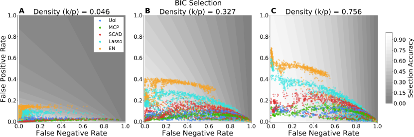
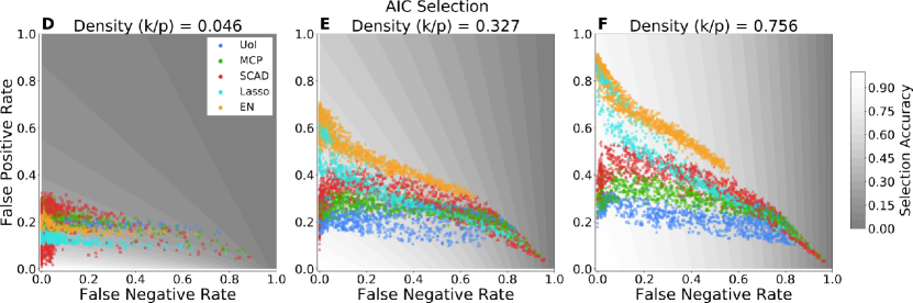
Figure 2: Scatter plots of the false negative rate vs. false positive rate for BIC selection (A-C) and AIC selection (D-F) across 3 different model densities (n/p ratio = 4, all signal to noise parameters included). Each scatter point represents a single fit. $\beta$ distributions are encoded in marker shapes (square: uniform distribution, triangular: inverse exponential distribution, circular: Gaussian distribution). Shaded regions represent regions of equal selection accuracy. The orientation of these regions for different model densities illustrates the differing contributions of false negatives vs. false positives, with false positive control being far more important for sparser models, and conversely false negatives being more important for denser models. Estimators can be seen to be characterized by specific tradeoffs between the false positive and false negative control, with SCAD/BIC/UoI (red/green/blue) controlling the false positive rate most aggressively, whereas Elastic Net (orange) controls for false negatives more effectively. The tails of the scatter points extending towards the bottom right of the plot are comprised of the model designs with smallest $\alpha$.

4.1 False Positive/False Negative Characteristics

We first visualized support selection performance across estimators by scattering the false negative rate vs. false positive rate of each fit for several representative model densities (Figure 2 for BIC and AIC selection, Figure LABEL:s:fnrfprscatter for other criteria). Each scatter point represents the selection characteristics of fits to a distinct model design averaged over its 20 instantiations. The boundaries of the grayscale partitions of the false positive false negative rate plane correspond to contours of equal selection accuracy. The rotation of these contours with the true underlying model density reflects the relative importance of false negative and false positive control in modulating selection accuracy. Specifically, rotation towards the horizontal implies larger sensitivity to false positives, while conversely rotation towards the vertical implies greater sensitivity towards false negatives.

The accuracy of estimators exhibited clear structure that depends on the characteristics of the model design described above. We observe in panel A of Figure 2 that estimators that more aggressively promote sparsity (SCAD, MCP, UoI in red, green, and dark blue, respectively) featured better selection accuracy at low model densities (i.e. scatter points for these estimators lie in the white to light gray shaded regions), whereas those that control false negatives less aggressively, namely the Elastic Net (orange) and to a lesser extent the Lasso (cyan), fared better in denser true models (panel C). The scatter points for each estimator formed bands that span the false negative rate. This banding effect was most pronounced for SCAD/MCP/UoI.

Comparing the BIC selection (Figure 2 A-C) to AIC (Figure 2 D-F), these scatter plots also revealed that varying model selection methods also systematically shifted false negative/false positive characteristics of estimators. Selection methods with lower complexity penalties (i.e., AIC, CV) lifted the bands up along the false positive direction. Comparing the location of the blue/red/green scatter points between panels B and E, for example, we note that this effect was most dramatic for the set of estimators that most aggressively control false positives (SCAD/MCP/UoI). Consequently, similar tradeoffs as described before arose, with empirically better selection accuracy when models are dense obtained for AIC/CV, and vice versa for larger complexity penalties (BIC). The gMDL and eB methods behaved similarly to BIC (although there are a few exceptions to this, Figures LABEL:s:fnrfprscatter). We conclude that the choice of estimator and model selection criteria are both important in determining the false positive/false negative rate behavior of inference strategies.

4.2 $\alpha$-dependence of False Positives/False Negatives

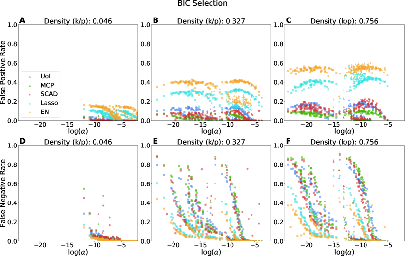
Figure 3: Scatter plot of the false positive rate (A-C) and the false negative rate (D-F) vs. $\alpha$ for each estimator using BIC as a selection criteria for three different model densities. $\beta$ distributions are encoded in marker shapes (square: uniform distribution, triangular: inverse exponential distribution, circular: Gaussian distribution). The false positive rate is only weakly modulated by $\alpha$, but is ordered by estimator, with MCP/SCAD/UoI consistently having the lowest false positive rates, Lasso intermediate, and the Elastic Net having the highest false positive rates. The effect becomes pronounced at higher model densities (panel C). For the false negative rates, scatter points follow a characteristic sigmoidal profile, with a region of stable selection accuracy at low correlation (high $\alpha$), followed by an transition point of $\alpha$ after which the selection accuracy montonically decreases. The effect is again most visible at higher model densities. At model density 0.046 (panel D), all estimators are reasonably robust to decreasing alpha.

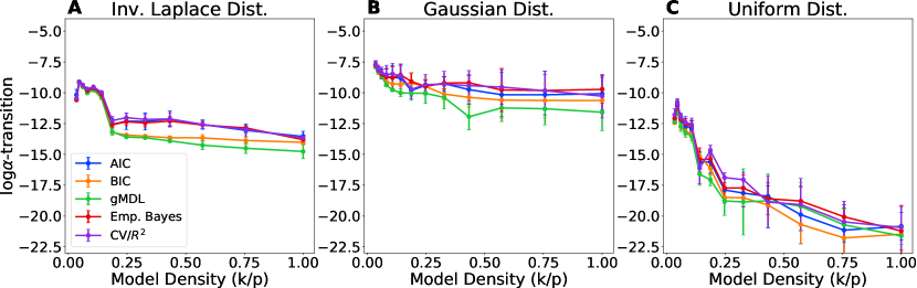
Figure 4: Plot of the $\alpha$-transition point associated with an inference algorithm’s false negative rate as a function of model density, separated by $\beta$ distribution and selection method. Errorbars are standard deviations taken across repetitions and estimator. The different numerical regimes of the $\alpha$-transition (highest in panel B, intermediate in panel A, and lowest in panel C) is attributable to the different characteristic value of $\beta_{\text{min}}$ for the different $\beta$ distributions.

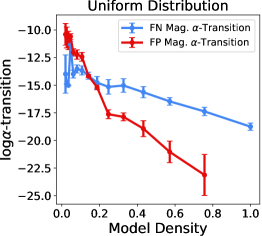
Figure 5: Plot of the average $\alpha$ transition point for estimation distortion across all inference algorithms and selection methods vs. model density for signal case 1. Errorbars represent standard deviation. After a model density of $>$ 0.15, the transition generally occurs at lower correlations (smaller $\alpha$) for the false negative magnitude. Furthermore, the variance across inference algorithms is consistently smaller for false negatives as opposed to false positives.

Recalling that the parameter $\alpha$ tunes the difficulty of the selection problem, we scattered the false positive and false negative rate vs. $\alpha$ for each inference algorithm across different model densities. A representative set of such plots for BIC selection is shown in Figure 3; other selection methods are shown in Figures SLABEL:s:fnr_alphascatter_gMDL-LABEL:s:fnr_alphascatter_CV. There was broadly large variation in performance modulated by the selection method employed. Furthermore, $\beta$-distributions are separately resolvable due to their different typical values of $\beta_{\text{min}}$. For example, in Figure 3F, for each estimator, the uniform distribution scatter points (squares) lie to the left of the inverse exponential distribution (triangular), which in turn lies to the left of the Gaussian distribution (circular).

In line with Figure 2, the false positive rate was not modulated by $\alpha$ (Figure 3 A-C). In fact, for some estimators, the highest false positive rate was achieved for intermediate $\alpha$, followed by a decline in false positive rate for smaller $\alpha$ (e.g. Lasso in Figure 3C). The false positive rate is instead a characteristic of each estimator. The SCAD/MCP/UoI class of estimators achieved lower false positives than Lasso, which in turn featured lower false positives than the Elastic Net. Model selection criteria can also be classified into a set that led to low false positive rates (gMDL, empirical Bayes, and BIC) vs. those that lead to high false positive rates (AIC, CV), although the Elastic Net with empirical Bayes selection featured the highest false positive rate of any inference algorithm (Supplementary Figure LABEL:s:fnr_alphascatter_eb, panels A-C).

On the other hand, the false negative rate scatter points, when separated by $\beta$-distribution, featured consistent behavior across inference algorithms. Focusing on BIC selection (Figure 3), all estimators achieved low false negative rates at the low model densities (Figure 3D). At intermediate model densities (Figure 3E), the false negative rate remained low until $\log\alpha$ became sufficiently small, at which point it rapidly increases. This value of $\log\alpha$ varied by $\beta$-distribution due to the differing characteristic values of $\beta_{\text{min}}$, occuring around $\log\alpha\approx-7.5$ for the Gaussian distribution at model density 0.327, $\approx\log\alpha=-10$ for the inverse exponential distribution, and $\approx\log\alpha=-15$ for the uniform distribution. Otherwise, this transition point is fairly universal across inference algorithms.

To produce summary statistics of false negative rates across model densities, selection methods, and n/p ratio/SNR cases, we fit sigmoidal curves to data for each inference algorithm and for each $\beta$ distribution. The sigmoid curve is described by 4 parameters:

$$S(\alpha)=c+\frac{a}{1+\exp(-b(\alpha-\alpha_{0}))}$$

In particular, we use the fitted value for the sigmoid midpoint $\alpha_{0}$, which we refer to as the $\alpha$-transition point, to quantify the value of $\alpha$ at which false negative rate has begun to increase appreciably. We found a large degree of universality in this transition point across estimators and selection methods. In Figure 4 we have averaged curves across estimators and plotted the mean and standard deviation of the resulting $\alpha$ transition points. Colors now represent each selection method. The curves for each selection method were strikingly similar within a $\beta$ distribution, with small standard deviations within each selection method indicating universality across estimators. The decrease of the $\alpha$-transition point with increasing model density can be explained by the overall shift of $\alpha$ towards smaller values due to the increase of $\rho(\Sigma,k)$ with $k$.

In the preceding analysis we treated false positives and false negatives as hard thresholded quantities. On the other hand, one can ask whether false negatives primarily arise from setting support elements with small signal strength to zero, and conversely whether false positives are associated with small coefficient estimates. Thus, while exact model support recovery in most cases is unattainable, one would hope that support inconsistencies produce low distortion of the desired coefficient vector. To this end, we calculate the average magnitude of false negatives and false positives, and normalize these quantities by the average magnitude of ground truth $\beta$. Raw scatter plots of these quantities ordered by $\alpha$ can be found in Figures LABEL:s:BIC_fnfp-LABEL:s:cv_fnfp. In the case of false negative magnitudes, we focus on the uniform $\beta$ distribution, as this provides the most “edge” cases of small coefficient magnitudes. We found that at low correlations, the hoped for low distortion effect largely holds true, but that there is an $\alpha$ transition point for both false negative and false positives after which significantly larger ground truth $\beta_{i}$ are selected out, and erroneously selected $\beta_{i}$ are assigned much larger values relative to the true signal mean. This transition point was again universal across all inference strategies (panels E, F, within each of Figures LABEL:s:BIC_fnfp-LABEL:s:cv_fnfp)

In Figure 5, we plot the transition point as a function of model density averaged across all estimators, selection criteria, and fit repetitions. For model densities $>0.15$, the transition point occurs at much smaller correlation strengths for the false negative distortions than the false positive distortions. Furthermore, the variance in the location of this transition point for false negative distortions is much smaller than for false positive distortions. For dense, correlated, models in cases 2 and 3 (SNR starved and sample starved, respectively), we find that the mean false positive magnitude can be as high as 5-10 times the true signal mean (e.g. Figure LABEL:s:BIC_fnfpC).

Overall, these results highlight the usefulness in the parameter $\alpha$, which emerges out of tail bounds on the performance of the exhaustive maximum likelihood decoder, as a quantifier of the difficulty of a sparse regression problem. The value of $\alpha$ at which the false negative rate of inference strategies begins to degrade was found to be universal. A similar universal transition point was found in the value of $\alpha$ at which false negatives and false positives begin to lead to large distortion of in magnitude of non-zero $\beta$ coefficients.

4.3 Overall Selection Accuracy

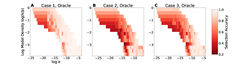
Figure 6: Oracle selection accuracy as a function of the log model density and $\alpha$ for each of the 3 signal cases described in Section 3. Each pixel in the colormap is the maximum oracle performance across all estimators for the particular combination of density and $\alpha$. For ideal signal characteristics in Case 1 (panel A), near perfect support recovery is in principle possible for a broad range of correlation strengths for models with density $<$ 0.15. The similar oracle selection accuracies between cases 2 and 3 (panels B and C) suggest that the sample starved and signal starved regression problems behave similarly. As compared to Case 1, worst case performance for intermediate model densities $>0.1$ and $<0.5$ is lower, especially for large correlations. For the densest models ($>0.5$), oracle performance is relatively insensitive to correlation strength, reflecting the insensitivity of the FPR to $\alpha$. Near-perfect support recovery is empirically still possible for the sparsest models (density $<0.05$).

An inference algorithm deployed in practice must employ both an inference estimator and model selection criteria. We have therefore determined what the best performing combination is as a function of underlying model density and $\alpha$. To set an overall scale for these comparisons, one can use an oracle selection criteria that simply chooses the support along a regularization path of maximum selection accuracy. For each value of $\alpha$ and model density, the maximum of this oracular selection across all estimators gives a proxy for the best achievable selection accuracy in principle at finite sample size and SNR.

In Figure 6 we plot the oracle selector for each signal case. In the ideal signal and sample size case (case 1), the oracle selector was able to achieve near perfect selection accuracy in the fully dense models (top row, panel C) and those models with with density $<0.14$ (log model densities $<-2$) even in model designs with very small $\alpha$. The oracle selector suffered moderate loss of selection accuracy in intermediate model densities for model designs with small $\alpha$ (darker orange regions of panel C). A similar structure is present in the adequate sample but high noise and low sample size but adequate SNR cases (cases 2 and 3 in panels B and C, respectively), but the magnitude of selection accuracy performance loss and regions of $\alpha$ and model densities for which the loss occurred expanded. In particular, only in the very sparsest models (density $<0.05$, log model density $<-3$) with larger $\alpha$ was perfect selection possible in principle.