Ice-Coated Pebble Drift as a Possible Explanation for Peculiar Cometary CO/H2O Ratios

Abstract

To date, at least three comets — 2I/Borisov, C/2016 R2 (PanSTARRS), and C/2009 P1 (Garradd) — have been observed to have unusually high CO concentrations compared to water. We attempt to explain these observations by modeling the effect of drifting solid (ice and dust) material on the ice compositions in protoplanetary disks. We find that, independent of the exact disk model parameters, we always obtain a region of enhanced ice-phase CO/H2O that spreads out in radius over time. The inner edge of this feature coincides with the CO snowline. Almost every model achieves at least CO/H2O of unity, and one model reaches a CO/H2O ratio $>10$. After running our simulations for 1 Myr, an average of 40% of the disk ice mass contains more CO than H2O ice. In light of this, a population of CO-ice enhanced planetesimals are likely to generally form in the outer regions of disks, and we speculate that the aforementioned CO-rich comets may be more common, both in our own Solar System and in extrasolar systems, than previously expected.

1 Introduction

Comets provide a unique window onto the ice-phase chemistry of a protoplanetary disk. These frozen remnants are generally considered to be the most pristine record available for understanding disk midplanes’ compositions. The chemical species present in solar system comets and their relative abundances provide unique and detailed insights into the protoplanetary disk that formed our planetary system (Mumma & Charnley, 2011; Altwegg & Bockelée-Morvan, 2003), and, more recently with the discoveries of passing extrasolar comets (Strøm et al., 2020), other planetary systems.

Water is typically the most abundant volatile species in cometary nuclei, with carbon monoxide comprising between about 0.2% to 23% relative to water, with a typical value around 4% (Bockelée-Morvan & Biver, 2017). However, at least three notable exceptions have been observed. Specifically, the interstellar comet 2I/Borisov was measured to have CO/H2O between 35% and 173% (Cordiner et al., 2020; Bodewits et al., 2020), significantly higher than the average cometary values for the Solar System. Bodewits et al. (2020) suggest 2I/Borisov’s composition could be explained by an unusual formation environment beyond the CO snowline, and, statistically, it is more likely that 2I/Borisov is a typical comet for its system. However, given the ubiquity of water in interstellar clouds (Boogert et al., 2015), it would be challenging to have a scenario with CO ice freezing out without abundant water ice, which has a higher binding energy than CO. At least two additional comets, C/2009 P1 (Garradd) and C/2016 R2 (PanSTARRS), which originate in our own solar system, have high CO abundances as well: C/2009 P1 (Garradd) has a CO production rate of 63% that of water (Feaga et al., 2014), and C/2016 R2 (PanSTARRS) has an even higher CO production rate than 2I/Borisov (Biver et al., 2018; McKay et al., 2019). Although these comets represent a very small fraction of the comets for which CO/H2O has been measured, they are more difficult to explain. Therefore we need a mechanism that can both create enhanced CO to H2O ratios compared to interstellar or disk-averaged CO/H2O abundance ratios and create a spread of CO to H2O within a disk like our solar nebula.

What kinds of mechanisms could explain these unusual compositions both interior and exterior to our solar system? Biver et al. (2018) suggest that C/2016 R2 could be a piece of a differentiated comet; Cordiner et al. (2020) suggest the same for 2I/Borisov. De Sanctis et al. (2001) found that CO and other volatiles could almost be completely absent in the upper layers of a hypothetical differentiated comet; in this scenario, 2I/Borisov and C/2016 R2 could be pieces of the cores of such differentiated comets. Alternatively, the chemistry of the planet-forming disk could evolve over time to create exotic compositions at different disk locations. For example, Eistrup et al. (2019) consider several comets and attempt to reproduce their molecular abundances with a model protoplanetary disk. Their disk model produces a maximum CO/H2O ratio of about $1\%$ over a range of disk radii from $15$ au to $30$ au from the central star. However, to reproduce a comet like 2I/Borisov, we would require a ratio that could be as high as $100\%$.

In recent years, dust transport, especially radial drift, has been found to be an important factor in shaping the solid mass distribution in disks (Testi et al., 2014; Piso et al., 2015; Öberg & Bergin, 2016; Cridland et al., 2017). If the timing of volatile freeze out and dust transport due to, e.g., drift, are not synced, it could become possible to create a variety of ice compositions purely due to dust dynamics.

In this paper, we explore whether a comet such as 2I/Borisov or C/2016 R2 (PanSTARRS) could form in a pocket of CO-rich material in an otherwise H2O-rich disk as a result of dust transport, and under what conditions such pockets could form. The paper is structured as follows. In Section 2, we explain the equations and software used to define our disk model. Section 3 presents our calculated CO/H2O ice ratios across a generic protoplanetary disk. We discuss the implications of these results in light of the recent findings of comets and an exo-comet with high CO abundance in Section 4 and conclude in Section 5.

The authors note that a similar paper (Mousis et al., 2021) appeared independently during the review process for this paper.

2 Methods

Our goal is to globally simulate the surface densities of solids and gas in a protoplanetary disk, incorporating simple adsorption and desorption processes for the chemical species we consider, H2O and CO. We build on the physical models of disk gas and dust following Lynden-Bell & Pringle (1974) and Birnstiel et al. (2010). In addition, we take into account the time evolving disk temperature due to the pre-main sequence stellar evolution over the time scales of our model simulation. The following sections detail these model components.

2.1 Gas dynamics

To model the dynamics of the gas bulk (defined as the bulk hydrogen gas, which experiences no source terms), we follow Lynden-Bell & Pringle (1974), which is based on the $\alpha$-disk model of Shakura & Sunyaev (1973). Thus, we have the partial differential equation

$$\frac{\partial\Sigma_{\mathrm{gas}}}{\partial t}-\frac{3}{R}\frac{\partial}{\partial R}\left[R^{1/2}\frac{\partial}{\partial R}\left(\nu\Sigma_{\mathrm{gas}}R^{1/2}\right)\right]=0$$ (1)

in the absence of sources and sinks, where $\Sigma_{\mathrm{gas}}\equiv\int\rho_{\mathrm{gas}}\mathop{}\!\mathrm{d}z$ is the surface density of gas, $\nu$ is the viscosity, $R$ is the distance from the star in the $x$-$y$ plane, and $t$ is time. Viscosity is, in turn, given by

$$\nu=\alpha c_{s}^{2}/\Omega$$ (2)

where $\alpha$ is a small parameter of our choosing, typically set to $10^{-4}$ to $10^{-2}$; $c_{s}$ is the local sound speed, given by

$$c_{s}=\sqrt{\frac{k_{B}T}{\mu m_{p}}},$$ (3)

where $k_{B}$ is Boltzmann’s constant, $T$ is the local temperature, $\mu$ is the mean molecular weight, and $m_{p}$ is the proton mass; and $\Omega$ is the Keplerian angular frequency,

$$\Omega=\sqrt{\frac{GM_{\star}}{R^{3}}},$$ (4)

with $G$ the gravitational constant and $M_{\star}$ the central stellar mass. Equations 1, 2, 3, and 4 completely define the model of the gas bulk given parameters $\mu$, $M_{\star}$, and $\alpha$; the local temperature field $T=T\!\left(R,t\right)$ (see Section 2.4; and the initial condition $\Sigma_{\mathrm{gas}}\!\left(R,t=0\right)$.

For the initial condition, we first define the self-similar solution,

$$\Sigma_{\mathrm{ss}}\!\left(R\right)=\Sigma_{c}\left(\frac{R}{R_{c}}\right)^{-\gamma}\exp\!\left[-\left(\frac{R}{R_{c}}\right)^{2-\gamma}\right],$$ (5)

with $\Sigma_{c}=20~{}\text{\text{g}}~{}\text{\text{cm}\textsuperscript{$-2$}}$, $R_{c}=20~{}\text{\text{au}}$, and $\gamma=0.5$; for reference, Andrews et al. (2012) uses $-1\leq\gamma\leq 1$. Here, $\Sigma_{c}$ is the surface density at radius $R_{c}$, and $\gamma$ determines the slope of the power law part of the solution. Unfortunately, when $R\ll R_{c}$, this solution begins to blow up, which makes it computationally difficult to handle. We use a smooth interpolation between the self-similar solution and a flat, constant surface density profile, given by

$$\Sigma_{\mathrm{gas}}\!\left(R,t=0\right)=\left(\Sigma_{\mathrm{ss}}\!\left(R\right)^{-p}+\Sigma_{\mathrm{ss}}\!\left(R_{\mathrm{trans}}\right)^{-p}\right)^{-1/p}$$ (6)

as our initial condition. We take $p=5$ and $R_{\mathrm{trans}}=1~{}\text{\text{au}}$ so that the transition occurs close to the interior of the domain and the transition from the self-similar to the flat profile is not too sharp.

Though we have chosen to work in one dimension, some quantities depend on the local density $\rho$ rather than the surface density $\Sigma$. In these cases, we assume a vertical Gaussian distribution of material,

$$\rho\!\left(R,z\right)=\frac{\Sigma\!\left(R\right)}{\sqrt{2\pi}h_{\mathrm{gas}}}\exp\!\left[-\frac{1}{2}\left(\frac{z}{h_{\mathrm{gas}}}\right)^{2}\right]$$ (7)

where the scale height $h_{\mathrm{gas}}=c_{s}/\Omega$.

2.2 Dust dynamics

We consider two solid populations in our model: a small “dust” population with radius $0.1$ µm and a “pebble” population with radius $1$ mm, with mass ratios $90\%$ and $10\%$, respectively. Following Birnstiel et al. (2010), we define the surface density evolution for each population by the partial differential equation

$$\frac{\partial\Sigma_{\mathrm{solid}}}{\partial t}+\frac{1}{R}\frac{\partial}{\partial R}\left(RF_{\mathrm{tot}}\right)=0$$ (8)

in the absence of sources and sinks, where $\Sigma_{\mathrm{solid}}$ is the solid surface density for a single population and $F_{\mathrm{tot}}\equiv F_{\mathrm{adv}}+F_{\mathrm{diff}}$ is the total flux, with contributions from an advective and diffusive part. The fluxes are given by

$$F_{\mathrm{adv}}=\Sigma_{\mathrm{solid}}u_{\mathrm{solid}}$$ (9)

and

$$F_{\mathrm{diff}}=-\frac{\nu}{\mathrm{St}^{2}+1}\frac{\partial}{\partial R}\left(\frac{\Sigma_{\mathrm{solid}}}{\Sigma_{\mathrm{gas}}}\right)\Sigma_{\mathrm{gas}}.$$ (10)

In the above equations, the Stokes number is given by

$$\mathrm{St}=\frac{\pi}{2}\frac{a_{\mathrm{gr}}\rho_{\mathrm{gr}}}{\Sigma_{\mathrm{gas}}}$$ (11)

in the Epstein regime, with $a_{\mathrm{gr}}$ the radius of a single (pebble or dust) grain and $\rho_{\mathrm{gr}}$ the density of the solid material (i.e., silicate). The radial velocity of the solids is given by

$$u_{\mathrm{solid}}=\frac{u_{\mathrm{gas}}}{\mathrm{St}^{2}+1}-\frac{2u_{\mathrm{grad}}}{\mathrm{St}+\mathrm{St}^{-1}}$$ (12)

where

$$u_{\mathrm{gas}}=-\frac{3}{R^{1/2}\Sigma_{\mathrm{gas}}}\frac{\partial}{\partial R}\left(R^{1/2}\nu\Sigma_{\mathrm{gas}}\right)$$ (13)

is the gas velocity and

$$u_{\mathrm{grad}}=-\frac{E_{d}}{2\rho_{\mathrm{gas}}\Omega}\frac{\partial p_{\mathrm{gas}}}{\partial R}$$ (14)

is the velocity due to the gas pressure gradient. $E_{d}$ is a drift efficiency parameter and $p_{\mathrm{gas}}=\rho_{\mathrm{gas}}c_{s}^{2}$ is the gas pressure. Birnstiel et al. (2010) gives more detail on these equations.

Again, we must make some assumption about the vertical distribution of solids to determine $\rho_{\mathrm{solid}}$. We make the same vertical Gaussian assumption as for the gas, but, to simulate settling, we allow the scale height of the pebbles to be a fraction $\xi_{\mathrm{pebbles}}$ of the gas scale height, so $h_{\mathrm{pebbles}}=\xi_{\mathrm{pebbles}}h_{\mathrm{gas}}$. We use $\xi_{\mathrm{dust}}=1$ such that the dust is not settled. For the pebbles, we take $\xi_{\mathrm{pebbles}}=0.1$.

2.3 Adsorption and desorption

Finally, adsorption, the process by which atoms and molecules stick to a solid surface, and desorption, in which the atoms and molecules leave the surface, must be included as source terms. Hollenbach et al. (2009) gives the adsorption timescale as

$$\tau_{\mathrm{ads}}=\left(n_{\mathrm{solid}}\sigma_{\mathrm{gr}}v_{\mathrm{therm}}\right)^{-1}$$ (15)

where $n_{\mathrm{solid}}$ is the local number density of solids, $\sigma_{\mathrm{gr}}=\pi a_{\mathrm{gr}}^{2}$ is the cross-sectional area of a single grain, and $v_{\mathrm{therm}}=\sqrt{8k_{B}T/\pi m}$ is the thermal velocity of the atom or molecule of interest. Inverting the timescale, we find the adsorption rate

$$R_{\mathrm{ads}}=n_{\mathrm{solid}}\sigma_{\mathrm{gr}}v_{\mathrm{therm}}$$ (16)

per atom or molecule.

For desorption, Hollenbach et al. (2009) gives the rate per molecule of ice

$$R_{\mathrm{des}}=\nu_{\mathrm{att}}\exp\!\left(-\frac{T_{\mathrm{bind}}}{T}\right),$$ (17)

where $\nu_{\mathrm{att}}$ is the attempt frequency — the vibrational frequency of the atoms and molecules on the surface — of order $10^{12}$ s^$-1$, and $T_{\mathrm{bind}}$ is the binding energy of the species of interest (4800 K for H2O and 960 K for CO, Aikawa et al. 1996).

Combining Equations 16 and 17, we find the volumetric source terms

$$s_{\mathrm{gas}}=R_{\mathrm{des}}n_{\mathrm{solid}}-R_{\mathrm{ads}}n_{\mathrm{gas}}.$$ (18)

To find the appropriate source term for the surface density equations above, we must integrate $s_{\mathrm{gas}}$ vertically and multiply by the species’ mass $m$. We find

$$S_{\mathrm{ads}}=\frac{\sigma_{\mathrm{gr}}v_{\mathrm{therm}}\Sigma_{\mathrm{gas}}\Sigma_{\mathrm{solid}}}{\sqrt{2\pi}m_{\mathrm{gr}}h_{\mathrm{gas}}\sqrt{1+\xi_{\mathrm{solid}}^{2}}}.$$ (19)

and

$$S_{\mathrm{des}}=m\int\limits_{-\infty}^{\infty}R_{\mathrm{des}}n_{\mathrm{solid}}\mathop{}\!\mathrm{d}z=R_{\mathrm{des}}\Sigma_{\mathrm{solid}}.$$ (20)

(Equation 19 is derived in Appendix A.1.) These source terms both have units of g cm^$-2$ s^$-1$ and represent the rates at which the surface density changes due to adsorption and desorption processes, respectively.

Thus, the source terms for surface density equations are given by

$$S_{\mathrm{gas}}=S_{\mathrm{des}}-S_{\mathrm{ads}}$$ (21)

and

$$S_{\mathrm{solid}}=S_{\mathrm{ads}}-S_{\mathrm{des}}.$$ (22)

These source terms encode the rate at which the surface densities of gas and solid species are changing due to the adsorption and desorption chemistry in our model.

2.4 Temperature structure

The temperature field presents a challenge by itself. Temperature appears in Equation 1 through the viscosity term, and so it contributes to the gas dynamics. Yet the gas dynamics play a role in determining the dust dynamics, which, through radiative transfer from the central star, determine the temperature. In addition, the intrinsic luminosity of the star is expected to change significantly over the timescales presented here (Siess et al., 2000). One way to solve this circular problem is through iteration, as in Price et al. (2020). However, that procedure would be more computationally costly when coupled to the code we have described here.

Instead of seeking a self-consistent solution, as in Price et al. (2020), we follow a simpler procedure to capture the approximate temperature structure. Noting that the bulk surface density, and therefore dust grain surface density, does not change significantly over time, we use RADMC-3D version 0.41 (Dullemond et al., 2012) to compute a temperature structure with a self-similar dust initial condition (i.e., same form as Equation 5), assuming a dust-to-gas ratio of $0.01$ and using the interpolated DSHARP opacities (Birnstiel et al., 2018). We note that this procedure is an approximation, since we are not taking into account the evolving dust and pebble surface density, but it provides sufficient accuracy for our proof-of-concept purposes.

Next, we fit a power law $T\propto R^{-\beta}$ to the output from RADMC-3D, limited to the region between 2 au and 20 au to avoid edge effects and unphysical behavior far from the star. Though we run RADMC-3D with two dust populations, the temperatures are virtually equal, so we assume a power law slope of $-0.41$ and appropriate intercept parameter, which reasonably captures the behavior of both populations, and use that same power law for both when solving the differential equations.

To take into account a changing stellar luminosity over time, we use the Siess et al. (2000) web server to compute stellar radii $R_{\star}$ and effective temperatures $T_{\mathrm{eff}}$ over the lifetime of the disk. Then, inspired by Chiang & Goldreich (1997), Equation 12, we see that the disk temperature scales by a factor $f\propto R_{\star}^{1/2}T_{\star}$. We compute this factor from the isochrons and scale it by the initial value such that $f\leq 1$ at all times, i.e., the disk temperature is decreasing over time, primarily due to radial contraction decreasing the bolometric luminosity of the central star.

Finally, we perform a fit to the two regimes we observe in $f$ — a flat, early-time regime and a sloped, late-time regime — and join the two regimes by smooth interpolation. This interpolation takes the same form as Equation 6, but with a parameter $p=100$ that is more appropriate for this data. See Figure 1 for the parameters in each regime and the final interpolation. Figure 2 shows the resulting temperature that is used in the fiducial model alongside two fixed-temperature models representing the beginning and end state.

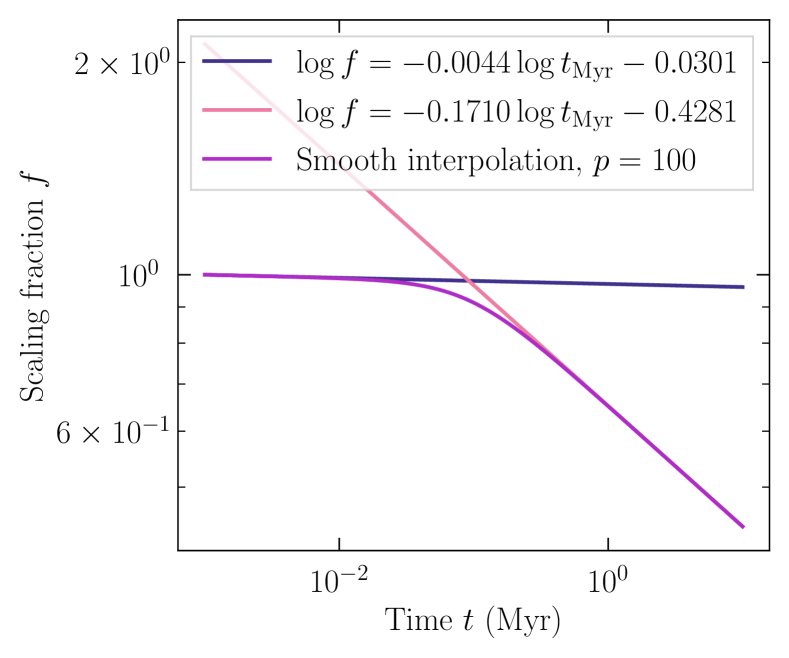
Figure 1: Temperature scaling fraction as determined by fitting Siess et al. (2000) isochrons with two power laws and then interpolating smoothly between them. The complete procedure is described in Section 2.4. The parameters of the lines are given in the legend, and the interpolation “power” $p$ is chosen to give a smooth curve to the intersection of the lines.

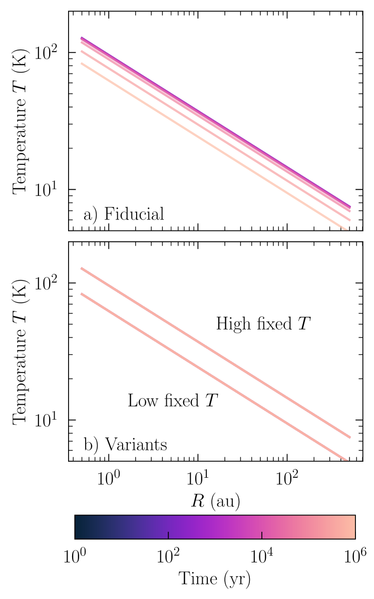
Figure 2: In panel (a), we show the temporal and spatial evolution of the disk temperature (assumed vertically invariant for the purposes of the model) for the fiducial case. In panel (b), we show the two variants explored: a high temperature case (upper) and low temperature case (lower), both of which are held fixed in time. The line color in all panels indicates logarithmically-increasing time.

2.5 Solution procedure

To solve Equations 1 and 8 with source terms given by Equations 21 and 22, we require approximations of first and second derivatives in radius. We use a logarithmically-spaced mesh in $R$ and second-order accurate finite difference derivatives estimated with Equations A3 and A4. Where appropriate, we switch to first-order accurate upwind finite difference derivatives.

To advance the solution in time, we use the backward differentiation formula (BDF) implementation in the Portable, Extensible Toolkit for Scientific Computation (PETSc) (Balay et al., 1997, 2019, 2020) time stepping (TS) (Abhyankar et al., 2018) module. We use the PETSc internal colored finite difference Jacobian and solve the resulting linear system with the MUltifrontal Massively Parallel sparse direct Solver (MUMPS) (Amestoy et al., 2001, 2019).

The system of partial differential equations we finally solve is in nine quantities. The bulk gas, pebble, and dust densities are treated according to Equations 1 and 8 with no source terms. Then, we consider H2O and CO in gas, as ice on pebbles, and as ice on dust grains by adding the appropriate source term to the right-hand sides of Equations 1 and 8. We evolve the equations to $1$ Myr on the spatial domain $\left[0.5~{}\text{\text{au}},500~{}\text{\text{au}}\right]$.

3 Results

Table 1: Various model cases and parameter values.

Identifier	Viscosity parameter $\alpha$	Drift efficiency $E_{d}$	Initial CO/H2O	Temperature model
Fiducial	$10^{-3}$	$0.1$	$20\%$	time-evolving
Low $\alpha$	$10^{-4}$	$0.1$	$20\%$	time-evolving
Low drift	$10^{-3}$	$0.01$	$20\%$	time-evolving
High drift	$10^{-3}$	$0.9$	$20\%$	time-evolving
Low CO	$10^{-3}$	$0.1$	$1\%$	time-evolving
High CO	$10^{-3}$	$0.1$	$100\%$	time-evolving
Low fixed $T$	$10^{-3}$	$0.1$	$20\%$	static, $t=1~{}\text{\text{Myr}}$
High fixed $T$	$10^{-3}$	$0.1$	$20\%$	static, $t=0~{}\text{\text{Myr}}$

3.1 Fiducial model

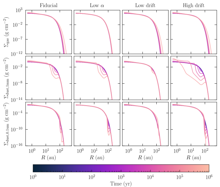
Figure 3: Temporal and spatial evolution of the three bulk surface densities for four selected model cases. The rows represent the surface densities of each type (gas, 1 mm pebbles, and 1 µm dust, from top to bottom, respectively) while the columns represent the different models. Temporal evolution is shown by the color gradient, which extends through time on a logarithmic scale from darker to lighter colors. The most notable feature is the development of a density deficit in the solids around 100 au caused by drift; this is observed in both pebbles and dust, but the pebbles exhibit a stronger effect because they drift more efficiently than the dust, which is well-coupled to the gas.

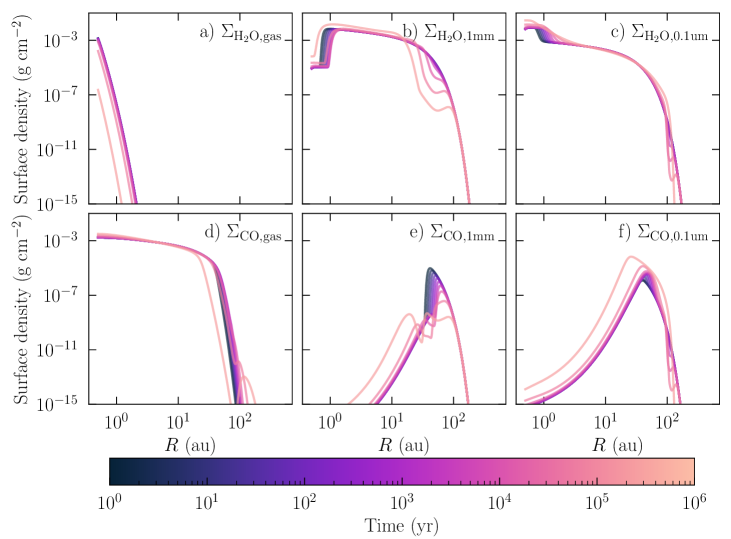
Figure 4: Fiducial model evolution of the surface densities of H2O (top row) and CO (bottom row) in the gas phase (left column) and solid phases (middle and right column). The pebble deficit from Figure 3 is echoed in the water ice, but the CO experiences a very different behavior than the bulk solids.

In Figure 3 (first column), we show the behavior of the bulk gas, pebbles, and dust over time and radius in the fiducial model. While the gas behavior shows simple viscous spreading, the pebbles and dust show more interesting behavior. The 1 mm pebbles form a shallow gap-like structure at about 30–100 au. This position coincides with the radius where the Stokes number goes to unity, and thus where the pebbles move fastest. As a result, at smaller radii, the pebbles move inward, and, at larger radii, the pebbles move outward, resulting in a pebble deficit at about 100 au. The 0.1 µm dust forms a similar structure at larger radii.

Figure 4 shows that the ice-coated solids do not universally follow the same trends as the bulk. While H2O on pebbles and dust forms the gap-like structure near 100 au, there is a second pebble and dust deficit at 1 au, the H2O snowline, where there is also a rapid increase in H2O vapor surface density. The behavior of CO is significantly different from that of H2O. The gap at $30$–$100$ au is much shallower, and only clearly visible at late times. Analogous to H2O, there is a rapid drop in CO dust and pebble surface density at the CO snowline. Figure 4 already shows a clear change in the CO/H2O surface density ratio in the outer disk.

In Figure 5, we present the main results of this paper both for the fiducial model and for a small parameter study (see next section). Each panel in the figure shows the evolution of the CO/H2O ratio in two ways: On the left, we show the variation over time and space on the vertical and horizontal axes, respectively. On the right, in a smaller panel, we integrate over radius in the region shown and show the evolution of the ice mass — total and where CO/H2O $\geq 1$ — over time. In Figure 5a, we show the predicted ratio of CO/H2O for our fiducial model, and we find that a maximum ratio near unity is achieved by 1 Myr in the region between about $20$ and $200$ au, and that this feature takes the shape of a funnel when observed in the space-time plane. This enhanced material accounts for an average of $40\%$ of the disk mass. See Table 3.2 for similar measurements of each model case that follows.

3.2 Parameter study

While our fiducial model results are encouraging in explaining anomalous, CO-enhanced comets, we also seek to understand the robustness of this result to changes in disk parameters, relatively unconstrained by observations or detailed simulations. The first parameters of interest are the viscosity parameter and drift efficiency. The viscosity parameter $\alpha$ ultimately sets the diffusion coefficient, which directly controls the gas’s diffusion and the diffusive flux of the solids. Figure 3 (second column) shows that reducing this parameter only has some minor effects on the dust and pebble evolution. The drift efficiency $E_{d}$ influences the coupling of solids to gas but only appears in the dust velocity, and therefore leaves gas motion unchanged. Figure 3 (third and fourth columns) show that increasing and decreasing this parameter dramatically changes the drift and therefore depletion of solids in the outer disk regions.

Figure 5b shows the enhancement of the CO/H2O ratio in ice for a model with $\alpha$ reduced by a factor of ten compared to the fiducial model. Reducing $\alpha$ makes the viscosity smaller everywhere, which, in turn, amounts to making the diffusion coefficient smaller. Thus, we would expect that disk material would experience less viscous spreading in this case, and, indeed, we see that the characteristic “funnel” shape of the CO-enhanced region in time and space is truncated and does not reach 100 au, while drift still carries material inward towards the star. The amount of CO-enhanced ice is modest, but it is certainly present.

In Figures 5c and 5d, we show the enhancement of the CO/H2O ratio in ice for the low and high drift models, respectively; for these test cases, we fixed $E_{d}$ at $0.01$ and $0.9$, changing the efficiency of the coupling to the gas pressure derivative. The models achieve about the same maximum CO/H2O ratio, but with very different fractions of CO-enhanced ice; i.e., the low-drift enhancement feature is visibly smaller in the space-time plane. We immediately see, then, that the efficiency of the radial drift of pebbles and dust is very important for predicting the amount of mass available for making comets like 2I/Borisov and C/2016 R2 (PanSTARRS). We return to this in the discussion section.

The third parameter of interest is the initial CO/H2O ratio. We test two possibilities in addition to the fiducial model: A high CO/H2O value of $100\%$ and a low CO/H2O value of $1\%$. We choose these end-member cases because, while typical comets have CO/H2O of about $4\%$ (Bockelée-Morvan & Biver, 2017), they may have $1\%$ or less (Mumma & Charnley, 2011), while the interstellar medium has up to $100\%$ with a large errorbar (Öberg, 2016). Note that the amount of CO has no effect on the bulk dynamics; it only affects the chemical evolution of the disk. In Figures 5e and 5f, we show the chemical evolution of the disk in these two cases. We find that the low CO model is not able to reach a CO/H2O ratio of unity; see Figure 5e. On the other hand, the high CO model easily reaches values of CO/H2O $\gtrsim 10$ by about $1$ Myr, as shown in Figure 5f, and this material accounts for a large fraction of the total disk mass.

The effect of a static, low temperature profile and a static, high temperature profile on our disk model is shown in Figures 5g and 5h, respectively. For these cases, we artificially fixed the temperature at its final or initial value, as appropriate (recall that the temperature strictly decreases with time, and see Figure 2 for the radially-dependent structures we adopted). These models reach roughly the same level of CO/H2O ice enhancement, but the radii where the enhancement occurs are shifted. In the low temperature model, the onset of the enhancement is delayed in time. The high temperature model’s enhanced region is shifted to larger radii because the disk is warmer everywhere, and so ice will desorb off the grains in this model farther out than in the fiducial model. Most importantly, the details of the temperature structure and evolution are not critical for the formation of a substantial amount of CO ice; both static temperature models achieve at least 30% CO-enhanced ice (see Table 3.2).

Finally, we summarize our results numerically in Table 3.2 in terms of maximum CO/H2O ratio, total number of CO-enhanced Halley-mass comets, and the mass fraction of the ice in the disk that is CO-enhanced by the end of the simulation. Most models achieve a CO/H2O ratio above unity (only the low CO model achieves a lower maximum ratio). The lowest ratio (low initial CO model) is just over $0.1$, and the largest ratio (high initial CO model) is greater than $10$, revealing a monotonic dependence on CO initial abundances. The low drift model produces the next-least amount of CO-enhanced ice. The fraction of ice in the region $\left[5~{}\text{\text{au}},200~{}\text{\text{au}}\right]$ that is CO-enhanced is, on average, about $40\%$, but in the high-drift model it is all of $87\%$, indicating that most water ice has been lost from the system due to pebble drift. The maximum number of CO-enhanced Halley-like comets that could be formed in the disks is between $10^{8}$ and $10^{10}$, though this assumes a formation efficiency of 100% from the dust and pebbles and no additional mixing, trapping, or drift. While a large range of values are possible, we emphasize that there is almost always a region where there is some CO ice enhancement relative to H2O ice.

Table 2: Model outcomes. Masses are measured over the same region shown in Figure 5.

Identifier	Highest CO/H2O ratio	Total CO-enhanced Halley-mass comets	Fraction of CO-enhanced ice
Fiducial	$2.39$	$6\times 10^{9}$	$48\%$
Low $\alpha$	$2.43$	$6\times 10^{9}$	$36\%$
Low drift	$2.21$	$2\times 10^{8}$	$6\%$
High drift	$2.56$	$6\times 10^{9}$	$87\%$
Low CO	$0.12$	–	$0\%$
High CO	$11.93$	$2\times 10^{9}$	$78\%$
Low fixed $T$	$3.47$	$6\times 10^{9}$	$35\%$
High fixed $T$	$2.96$	$2\times 10^{8}$	$30\%$

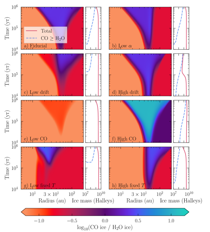
Figure 5: Evolution of the CO/H2O ice ratio as a function of time and space in the disk model. Each large panel represents a different set of conditions or parameters used, which can be found listed in Table 1. In each large panel, the two smaller panels show the evolution of the ice ratio (left, two-dimensional color plot) and the total mass in enhanced ice over time (right, line plot). In the line plot, the ice mass is measured in units of Halley’s comet’s mass, to give the reader an idea of how many comets could be formed from the material if formation was 100% efficient.

4 Discussion

We have explored the role of dust drift in changing the local ice composition in a protoplanetary disk midplane. Using models that assume simple ices composed of CO and H2O and allowing for adsorption and desorption, we find that parameters controlling the dynamics, such as the drift efficiency and viscosity, as well as the temperature (which affects dynamics indirectly), all play an important role in determining the specific amount of CO enhancement relative to H2O as well as the distribution of ices by 1 Myr. Yet, across our models, there is consistently a region of our disk that displays CO/H2O ice enhancement compared to the initial CO/H2O abundance ratio, independent of the choice of parameters, in all cases we have explored.

Why does this enhancement occur? Most of the water in our model is in the form of ice. Drift carries the water ice-laden pebbles and dust inward, creating an ice deficit. We can see from Figure 4 that the water ice deficit forms around 100 au and spreads out in time. Meanwhile, even though we start with CO as ice, interior to its snowline, it initially sublimates quickly. The gas-phase CO crosses the snowline as it viscously spreads out. This “new” CO enters the water ice deficit region and then freezes out onto whatever solids remain. In Figure 4c and 4f, we see that, while the amount of CO on pebbles decreases over time, the amount of CO on dust increases. The radial process we have described is similar to the “vertical cold finger effect” described by Meijerink et al. (2009), where water is depleted in the upper disk layers because of diffusive transport and settling. In addition, this work is consistent with the results of Ros & Johansen (2013), which found significant solid enhancement caused by transport across the radial snowline. This work demonstrates that there is likely to be a complex interplay with the evolution of solids and the chemical composition of the ice mantles they harbor. Future work should explore these connections with more advanced chemistry along with ice chemistry and/or isotopic chemistry, to fully understand the relationship between grain drift, viscous spreading across snowlines, and the resulting chemistry.

While we have limited ourselves in this paper to only two grain sizes, a more realistic simulation would use a continuous distribution of grain sizes. We expect that the largest grain size is the driving factor of the location of the inner edge of the enhancement feature. When the largest size is reduced from 1 mm, the largest size we considered here, drift becomes less efficient; when it is increased, drift becomes more efficient. Drift greatly influences the location of the inner edge of the “funnel” we observe in the models we present here. Since the mechanism proposed above only needs some small grain population to be entrained with the gas and some large population that drifts efficiently, we theorize that the exact distribution of grain sizes does not strongly influence our results.

5 Conclusions

We present models of the surface density evolution of a viscously-evolving protoplanetary disk, including the effect of grain drift, with the goal of explaining the observations of CO-enriched comets. To explore how midplane CO and H2O abundances in gas and ice evolve within this dynamic framework, we include simple adsorption and desorption chemistry to capture the interplay of dust transport and snowlines. We find that most of our disk models readily produce a region where CO ice is more abundant than H2O ice. These results indicate that forming CO-enriched comets may not be so unusual.

On the other hand, the fact remains that we have not observed very many CO-enriched comets to date. Assuming our Solar System originated with a nominal amount of CO, there may be some selection bias that causes CO-poor comets to be observed more frequently.

Fitzsimmons et al. (2019) and Xing et al. (2020) conclude that the extrasolar comet 2I/Borisov is in most ways — excluding its high CO/H2O ratio — similar to Solar System comets. Our results support the conclusion that the CO/H2O ice enhancement commonly occurs in the outer disk for solar-type stars, between $20$ and $100$ au. Perhaps comets that form so far out are more easily ejected due to being weakly gravitationally bound to their host star. 2I/Borisov may be an example of this mechanism at work. While dynamical simulations are beyond the scope of the present work, it would be interesting to compare the expected distribution of formation locations of extrasolar comets pre-ejection with the chemical patterns found here, to further test this hypothesis.

Appendix A Supplementary equations

A.1 Vertically-integrated source term

Since the evolution equations given in this paper are in terms of surface density, which is a vertically-integrated quantity, it is important to additionally vertically integrate the usual adsorption source term, as

$$S_{\mathrm{ads}}=m\int\limits_{-\infty}^{\infty}R_{\mathrm{ads}}n_{\mathrm{gas}}\mathop{}\!\mathrm{d}z =\sigma_{\mathrm{gr}}v_{\mathrm{therm}}\int\limits_{-\infty}^{\infty}\frac{\Sigma_{\mathrm{dust}}}{\sqrt{2\pi}h_{\mathrm{dust}}m_{\mathrm{gr}}}\exp\!\left[-\frac{1}{2}\left(\frac{z}{h_{\mathrm{dust}}}\right)^{2}\right]\frac{\Sigma_{\mathrm{gas}}}{\sqrt{2\pi}h_{\mathrm{gas}}}\exp\!\left[-\frac{1}{2}\left(\frac{z}{h_{\mathrm{gas}}}\right)^{2}\right]\mathop{}\!\mathrm{d}z$$ (A1)

$$=\frac{\sigma_{\mathrm{gr}}v_{\mathrm{therm}}\Sigma_{\mathrm{gas}}\Sigma_{\mathrm{dust}}}{\sqrt{2\pi}m_{\mathrm{gr}}h_{\mathrm{gas}}\sqrt{1+\xi_{\mathrm{dust}}^{2}}}.$$ (A2)

Note that we would have missed an important correction factor had we naïvely multiplied $n_{\mathrm{gas}}$ and $n_{\mathrm{dust}}$ without taking into account the vertical integration.

A.2 Finite difference approximations

On a finite grid in $x$ with points $\{x_{i}\}$, we use the modified finite difference formulae

$$\frac{\partial f}{\partial x}\approx\left(\frac{-h_{i+1}}{h_{i-1}\left(h_{i-1}+h_{i+1}\right)}\right)f_{i-1}+\left(\frac{1}{h_{i-1}}-\frac{1}{h_{i+1}}\right)f_{i}+\left(\frac{h_{i-1}}{h_{i+1}\left(h_{i-1}+h_{i+1}\right)}\right)f_{i+1}$$ (A3)

and

$$\frac{\partial^{2}f}{\partial x^{2}}\approx\left(\frac{2}{h_{i-1}\left(h_{i-1}+h_{i+1}\right)}\right)f_{i-1}+\left(\frac{-2}{h_{i-1}h_{i+1}}\right)f_{i}+\left(\frac{2}{h_{i+1}\left(h_{i-1}+h_{i+1}\right)}\right)f_{i+1},$$ (A4)

where $h_{i-1}=x_{i}-x_{i-1}$ and $h_{i+1}=x_{i+1}-x_{i}$, and $\{f_{i}\}$ are samples of a smooth function $f\!\left(x\right)$. These formulae are general and second-order accurate, and they apply to any irregularly-spaced grid.

References

- Abhyankar et al. (2018) Abhyankar, S., Brown, J., Constantinescu, E. M., et al. 2018, arXiv e-prints, arXiv:1806.01437. https://arxiv.org/abs/1806.01437
- Aikawa et al. (1996) Aikawa, Y., Miyama, S. M., Nakano, T., & Umebayashi, T. 1996, ApJ, 467, 684, doi: 10.1086/177644
- Altwegg & Bockelée-Morvan (2003) Altwegg, K., & Bockelée-Morvan, D. 2003, Space Sci. Rev., 106, 139, doi: 10.1023/A:1024685620462
- Amestoy et al. (2019) Amestoy, P. R., Buttari, A., L’Excellent, J.-Y., & Mary, T. 2019, ACM Trans. Math. Softw., 45, doi: 10.1145/3242094
- Amestoy et al. (2001) Amestoy, P. R., Duff, I. S., L’Excellent, J.-Y., & Koster, J. 2001, SIAM Journal on Matrix Analysis and Applications, 23, 15, doi: 10.1137/S0895479899358194
- Andrews et al. (2012) Andrews, S. M., Wilner, D. J., Hughes, A. M., et al. 2012, ApJ, 744, 162, doi: 10.1088/0004-637X/744/2/162
- Balay et al. (1997) Balay, S., Gropp, W. D., McInnes, L. C., & Smith, B. F. 1997, in Modern Software Tools in Scientific Computing, ed. E. Arge, A. M. Bruaset, & H. P. Langtangen (Birkhäuser Press), 163–202
- Balay et al. (2019) Balay, S., Abhyankar, S., Adams, M. F., et al. 2019, PETSc Web page, https://www.mcs.anl.gov/petsc. https://www.mcs.anl.gov/petsc
- Balay et al. (2020) —. 2020, PETSc Users Manual, Tech. Rep. ANL-95/11 - Revision 3.13, Argonne National Laboratory. https://www.mcs.anl.gov/petsc
- Birnstiel et al. (2010) Birnstiel, T., Dullemond, C. P., & Brauer, F. 2010, A&A, 513, A79, doi: 10.1051/0004-6361/200913731
- Birnstiel et al. (2018) Birnstiel, T., Dullemond, C. P., Zhu, Z., et al. 2018, ApJ, 869, L45, doi: 10.3847/2041-8213/aaf743
- Biver et al. (2018) Biver, N., Bockelée-Morvan, D., Paubert, G., et al. 2018, A&A, 619, A127, doi: 10.1051/0004-6361/201833449
- Bockelée-Morvan & Biver (2017) Bockelée-Morvan, D., & Biver, N. 2017, Philosophical Transactions of the Royal Society of London Series A, 375, 20160252, doi: 10.1098/rsta.2016.0252
- Bodewits et al. (2020) Bodewits, D., Noonan, J. W., Feldman, P. D., et al. 2020, Nature Astronomy, 4, 867, doi: 10.1038/s41550-020-1095-2
- Boogert et al. (2015) Boogert, A. C. A., Gerakines, P. A., & Whittet, D. C. B. 2015, ARA&A, 53, 541, doi: 10.1146/annurev-astro-082214-122348
- Chiang & Goldreich (1997) Chiang, E. I., & Goldreich, P. 1997, ApJ, 490, 368, doi: 10.1086/304869
- Cordiner et al. (2020) Cordiner, M. A., Milam, S. N., Biver, N., et al. 2020, Nature Astronomy, doi: 10.1038/s41550-020-1087-2
- Cridland et al. (2017) Cridland, A. J., Pudritz, R. E., & Birnstiel, T. 2017, MNRAS, 465, 3865, doi: 10.1093/mnras/stw2946
- De Sanctis et al. (2001) De Sanctis, M. C., Capria, M. T., & Coradini, A. 2001, AJ, 121, 2792, doi: 10.1086/320385
- Dullemond et al. (2012) Dullemond, C. P., Juhasz, A., Pohl, A., et al. 2012, RADMC-3D: A multi-purpose radiative transfer tool. http://ascl.net/1202.015
- Eistrup et al. (2019) Eistrup, C., Walsh, C., & van Dishoeck, E. F. 2019, A&A, 629, A84, doi: 10.1051/0004-6361/201935812
- Feaga et al. (2014) Feaga, L. M., A’Hearn, M. F., Farnham, T. L., et al. 2014, AJ, 147, 24, doi: 10.1088/0004-6256/147/1/24
- Fitzsimmons et al. (2019) Fitzsimmons, A., Hainaut, O., Meech, K. J., et al. 2019, ApJ, 885, L9, doi: 10.3847/2041-8213/ab49fc
- Hollenbach et al. (2009) Hollenbach, D., Kaufman, M. J., Bergin, E. A., & Melnick, G. J. 2009, ApJ, 690, 1497, doi: 10.1088/0004-637X/690/2/1497
- Lynden-Bell & Pringle (1974) Lynden-Bell, D., & Pringle, J. E. 1974, MNRAS, 168, 603, doi: 10.1093/mnras/168.3.603
- McKay et al. (2019) McKay, A. J., DiSanti, M. A., Kelley, M. S. P., et al. 2019, AJ, 158, 128, doi: 10.3847/1538-3881/ab32e4
- Meijerink et al. (2009) Meijerink, R., Pontoppidan, K. M., Blake, G. A., Poelman, D. R., & Dullemond, C. P. 2009, ApJ, 704, 1471, doi: 10.1088/0004-637X/704/2/1471
- Mousis et al. (2021) Mousis, O., Aguichine, A., Bouquet, A., et al. 2021, arXiv e-prints, arXiv:2103.01793. https://arxiv.org/abs/2103.01793
- Mumma & Charnley (2011) Mumma, M. J., & Charnley, S. B. 2011, ARA&A, 49, 471, doi: 10.1146/annurev-astro-081309-130811
- Öberg (2016) Öberg, K. I. 2016, Chemical Reviews, 116, 9631, doi: 10.1021/acs.chemrev.5b00694
- Öberg & Bergin (2016) Öberg, K. I., & Bergin, E. A. 2016, ApJ, 831, L19, doi: 10.3847/2041-8205/831/2/L19
- Piso et al. (2015) Piso, A.-M. A., Öberg, K. I., Birnstiel, T., & Murray-Clay, R. A. 2015, ApJ, 815, 109, doi: 10.1088/0004-637X/815/2/109
- Price et al. (2020) Price, E. M., Cleeves, L. I., & Öberg, K. I. 2020, ApJ, 890, 154, doi: 10.3847/1538-4357/ab5fd4
- Ros & Johansen (2013) Ros, K., & Johansen, A. 2013, A&A, 552, A137, doi: 10.1051/0004-6361/201220536
- Shakura & Sunyaev (1973) Shakura, N. I., & Sunyaev, R. A. 1973, A&A, 500, 33
- Siess et al. (2000) Siess, L., Dufour, E., & Forestini, M. 2000, A&A, 358, 593
- Strøm et al. (2020) Strøm, P. A., Bodewits, D., Knight, M. M., et al. 2020, arXiv e-prints, arXiv:2007.09155. https://arxiv.org/abs/2007.09155
- Testi et al. (2014) Testi, L., Birnstiel, T., Ricci, L., et al. 2014, in Protostars and Planets VI, ed. H. Beuther, R. S. Klessen, C. P. Dullemond, & T. Henning, 339, doi: 10.2458/azu_uapress_9780816531240-ch015
- van der Velden (2020) van der Velden, E. 2020, The Journal of Open Source Software, 5, 2004, doi: 10.21105/joss.02004
- Xing et al. (2020) Xing, Z., Bodewits, D., Noonan, J., & Bannister, M. T. 2020, ApJ, 893, L48, doi: 10.3847/2041-8213/ab86be