The three flavor revolution in fast pairwise neutrino conversion

Abstract

The modeling of fast flavor evolution of neutrinos in dense environments has been traditionally carried out by relying on a two flavor approximation for simplicity. In addition, vacuum mixing has been deemed negligible. For the first time, we highlight that the fast flavor evolution in three flavors is intrinsically different from the one obtained in the two flavor approximation. This is due to the exponential growth of flavor mixing in the $e$–$\mu$ and $e$–$\tau$ sectors generated by the vacuum term in the Hamiltonian. As a result, substantially larger flavor mixing is found in three flavors. Our findings highlight that the two flavor approximation is not justified for fast pairwise conversion, even if the angular distributions of non-electron type neutrinos are initially identical.

I Introduction

Flavor mixing is one of the least understood phenomena affecting the physics of neutrino-dense astrophysical sources, such as core-collapse supernovae and compact binary mergers. The flavor evolution can be significantly modified by the presence of a background medium, as first proposed by Mikheev, Smirnov, and Wolfenstein Mikheev and Smirnov (1986); Mikheyev and Smirnov (1985); Wolfenstein (1978). In addition, in neutrino-dense media, the forward scattering of neutrinos off their surrounding neutrino ensemble can crucially modify the flavor evolution in a non-linear fashion Pantaleone (1992); Sigl and Raffelt (1993). The flavor evolution induced by neutrino-neutrino interactions is correlated and often referred to as collective in nature. It is such that neutrinos of different energies change their flavor coherently.

More recently, it has been pointed out that the pairwise forward scattering of neutrinos of the form $\nu_{e}\bar{\nu}_{e}\leftrightarrow\nu_{x}\bar{\nu}_{x}$ (with $x=\mu,\tau$) can trigger collective flavor conversions, if the neutrino density is large enough Sawyer (2005, 2009, 2016); Chakraborty et al. (2016a, b); Tamborra and Shalgar (2021, in press). A necessary, although not sufficient, condition leading to the development of flavor mixing is the occurrence of crossings in the electron neutrino lepton number (ELN) Izaguirre et al. (2017). The development of fast pairwise conversions has been deemed to be not linked to the vacuum frequency of neutrinos; hence, pairwise conversion of neutrinos could occur even if the atmospheric neutrino mass-squared difference $\Delta m^{2}=0$ and should be independent on the neutrino energy $E$. However, it is shown in Ref. Shalgar and Tamborra (2021a) that the vacuum frequency $\Omega=\Delta m^{2}/2E\neq 0$ may strongly affect flavor mixing in the non-linear regime. Understanding the implications of fast pairwise conversion on the final flavor outcome is of relevance because fast conversions could have implications on the supernova explosion mechanism and on the synthesis of the heavy elements Xiong et al. (2020); Wu et al. (2017); George et al. (2020); Tamborra et al. (2017); Shalgar and Tamborra (2019); Abbar et al. (2019); Delfan Azari et al. (2019, 2020); Glas et al. (2020); Abbar et al. (2020); Nagakura et al. (2019); Morinaga et al. (2020); Capozzi et al. (2021); Abbar et al. (2021).

In order to grasp the behavior of neutrino collective oscillations, in analytical treatments and numerical simulations, a two flavor $(\nu_{e},\nu_{x})$ approximation has been classically adopted, as also considered above. This assumption was justified by the fact that significant flavor evolution of neutrinos is possible, if the neutrino self-interaction potential $\mu=\sqrt{2}G_{\textrm{F}}n_{\nu}$ (with $G_{\textrm{F}}$ being the Fermi constant and $n_{\nu}$ the neutrino number density) is much larger than the typical vacuum frequency $\Omega=\Delta m^{2}/2E$; the latter, in turn, is larger than the vacuum frequency due to the solar mass difference $\omega=\delta m^{2}/2E$ [note that two mass-squared differences differ by a factor $\mathcal{O}(30)$]. In addition, due to the typical energies of these astrophysical environments, the emission properties of $\nu_{\mu}$ and $\nu_{\tau}$ were assumed to be identical Duan et al. (2006a, b, c, 2007, 2010). As for slow neutrino self-interaction (exhibited by systems that are stable in the limit $\omega,\Omega\rightarrow 0$), the effects of $\Omega$ and $\omega$ on the collective flavor evolution could be factorized and the overall two flavor approximation has been deemed to be predictive of the final flavor outcome Fogli et al. (2009); Dasgupta et al. (2010a, b); Dasgupta and Dighe (2008); Dasgupta et al. (2008); Friedland (2010). In the case of fast flavor conversion, both vacuum frequencies have been neglected under the assumption that flavor mixing would be completely driven by the (anti)neutrino number density.

The $\nu_{\mu,\tau}=\bar{\nu}_{\mu,\tau}$ assumption has been challenged by the most recent supernova simulations allowing for muon production Bollig et al. (2017), and crossings have been found in the non-electron lepton number (nELN) distributions of neutrinos Capozzi et al. (2021). These developments have drawn attention on possible three flavor effects linked to fast pairwise conversion Airen et al. (2018); Chakraborty and Chakraborty (2020). In particular, Ref. Capozzi et al. (2020) has recently pointed out that the existence of large nELN crossings can vastly affect the flavor outcome.

In this work, we build on the findings of Ref. Shalgar and Tamborra (2021a) and expand on the ones of Refs. Airen et al. (2018); Chakraborty and Chakraborty (2020); Capozzi et al. (2020). For the first time, highlight the surprisingly strong dependence of the final flavor outcome on $\Omega$ and $\omega$ in the non-linear regime, even in the absence of zero nELN crossings considered in Ref. Capozzi et al. (2020); this may seem, at first, counter-intuitive, since $\omega\ll\Omega\ll\mu$. Our work highlights the limits of the usually adopted two flavor approximation and the strong dependence on vacuum flavor mixing: the main qualitative difference between the three and two flavor cases arises because the difference between $\nu_{\mu}$ and $\nu_{\tau}$ in the three flavor case grows exponentially, even if they are assumed to be identical or isotropic initially. This pins down the essence of three flavor effects and was not appreciated in Refs. Airen et al. (2018); Chakraborty and Chakraborty (2020); Capozzi et al. (2020). In addition, the non-trivial angular distributions for the non-electron type neutrinos effectively change the lepton number distribution and the onset of flavor mixing.

This paper is organized as follows. In Sec. II, we introduce the equations of motion and formulate the problem setup. In Sec. III, we compare the three flavor outcome to the two flavor scenario for the case where the non-electron neutrinos are only created through flavor mixing and for the scenario where crossings exist in the initial electron and muon neutrino lepton number distributions; we also explore the dependence of the flavor conversion physics on the neutrino mixing parameters. In Sec. IV, the effect of collisions on the flavor mixing phenomenology in three flavors is discussed. An outlook on our findings and conclusions are reported in Sec. V. The numerical convergence of the results presented in this work is discussed in Appendix A, together with the employed numerical techniques. The effect of the matter background on flavor mixing is discussed in Appendix B.

II Equations of motion and initial system configuration

The equations of motion are formally identical in two and three flavor systems–apart from the degrees of freedom. For each momentum mode $\vec{p}$ and in the two flavor approximation, the flavor state can be represented by a $2\times 2$ density matrix for neutrinos ($\rho$) and similarly for antineutrinos ($\bar{\rho}$). In the three flavor case, the density matrices are promoted to $3\times 3$ matrices which evolve in accordance to the following equations of motion in the mean-field approximation,

$$i\frac{d}{dt}\rho(\vec{p})=[H(\vec{p}),\rho(\vec{p})]\ \mathrm{and}\ i\frac{d}{dt}\bar{\rho}(\vec{p})=[\bar{H}(\vec{p}),\bar{\rho}(\vec{p})]\ .$$ (1)

We only consider an homogeneous neutrino gas, hence the total derivative with respect to time can be replaced by a partial derivative. The Hamiltonian receives contributions from the vacuum, matter, and the self-interaction terms:

$$H=H_{\textrm{vac}}+H_{\textrm{mat}}+H_{\nu\nu}\ ,$$ (2)

with

$$H_{\textrm{vac}} = \frac{1}{2E}UM^{2}U^{\dagger}\ ,$$ (3)

$$H_{\textrm{mat}} = \textrm{diag}(\lambda,0,0)\ ,$$ (4)

$$H_{\nu\nu}\ = \mu\int d^{3}\vec{p^{\prime}}[\rho(\vec{p^{\prime}})-\bar{\rho}(\vec{p^{\prime}})]\left(1-\frac{\vec{p}\cdot\vec{p^{\prime}}}{|\vec{p}||\vec{p^{\prime}}|}\right)\ .$$ (5)

The matrix $M$ represents the diagonal mass matrix, while $U(\theta_{12},\theta_{13},\theta_{23},\delta)$ is the PMNS matrix in the standard parametrization Zyla et al. (2020). The matter potential is $\lambda=\sqrt{2}G_{\textrm{F}}n_{e}$, where $n_{e}$ is the number density of electrons, and $\mu$ is the effective strength of the neutrino self-interaction, which is proportional to the neutrino number density. For antineutrinos, the Hamiltonian $\bar{H}$ has the same form as $H$, with $H_{\textrm{vac}}$ being replaced by $-H_{\textrm{vac}}^{\star}$.

In the numerical simulations, we assume the mixing parameters entering $H_{\textrm{vac}}$ reported in Table 1. In the following, we intend to compare the three flavor outcome with the two flavor one. To this purpose, we note that the three flavor system reduces to the two flavor approximation for $\theta_{12}=0$, $\theta_{23}=0$, and $\omega=0$.

Table 1: Default values of the vacuum mixing parameters adopted in our numerical simulations as from Ref. Zyla et al. (2020) for normal mass ordering.

Parameter	value
$\delta m^{2}$	$7.53\times 10^{-5}$ eV2
$\Delta m^{2}$	$2.45\times 10^{-3}$ eV2
$\theta_{12}$	$33.65^{\circ}$
$\theta_{13}$	$8.49^{\circ}$
$\theta_{23}$	$47.58^{\circ}$
$\delta$	$0.0$

In the two flavor approximation, it is common to ignore the matter effect and instead use a small mixing angle to take into account matter suppression effects Esteban-Pretel et al. (2008). This, however, has not been tested in the three flavor case in the context of fast conversions; hence, our numerical simulations include the matter potential and assume $\mu=\lambda=10^{5}$ km^-1, unless otherwise stated.

Apart from homogeneity, we also consider a system that is axially symmetric and, for simplicity, assume that the neutrino gas contains (anti)neutrinos with $E=50$ MeV to mimic the neutrino average energies just before decoupling. The neutrino momentum can thus be replaced by the cosine of the polar angle, $\cos\theta$, and both the density matrices and the Hamiltonian are independent of the spatial coordinates.

The fast flavor evolution depends on the angular distribution of (anti)neutrinos. At $t=0$

$$\rho_{ee}^{0}(\cos\theta) = 0.5$$ (6a)

$$\bar{\rho}_{ee}^{0}(\cos\theta) = 0.47+0.05\exp\left[-(\cos\theta-1)^{2}\right]\ ,$$ (6b)

as displayed in Fig. 1.

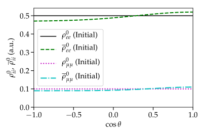
Figure 1: Initial angular distributions of electron neutrinos and antineutrinos. We assume an isotropic distribution for $\nu_{e}$ (black solid line) and a forward peaked distribution for $\bar{\nu}_{e}$ (dashed green line). For Case I, we set the distributions of non-electron type neutrinos to zero. For Case II, we use the angular distributions shown using the dotted and dash-dotted lines for the muon flavors with $a=10^{-2}$, while the distributions of the tau flavors remain zero.

For the non-electron flavors, we consider two scenarios: one with the angular distributions for non-electron (anti)neutrinos initially equal to zero (Case I) and one with the non-electron neutrino distributions different from zero (Case II). Hence, for Case I:

$$\rho_{\mu\mu}^{0}(\cos\theta) = \bar{\rho}_{\mu\mu}^{0}(\cos\theta)=0$$ (7a)

$$\rho_{\tau\tau}^{0}(\cos\theta) = \bar{\rho}_{\tau\tau}^{0}(\cos\theta)=0\ .$$ (7b)

For Case II:

$$\rho_{\mu\mu}^{0}(\cos\theta) = 0.1$$ (8a)

$$\bar{\rho}_{\mu\mu}^{0}(\cos\theta) = (0.1-a)+2a\exp\left[-2(\cos\theta-1)^{2}\right]\ ,$$ (8b)

where the parameter $a$ determines the magnitude of the crossing in the muon type neutrinos and we assume $a=0,10^{-3}$, and $10^{-2}$; see Fig. 1. In Case II, we assume $\rho_{\tau\tau}^{0}(\cos\theta)=\bar{\rho}_{\tau\tau}^{0}(\cos\theta)=0$. For the interested reader, details on the numerical solution of the neutrino equations of motion and their convergence are provided in Appendix A.

III Flavor mixing in two versus three flavors

In this section, we explore the flavor mixing in the two and three flavor scenarios for Cases I and II. We also discuss the effect of the vacuum mixing parameters on the flavor conversion physics.

III.1 Case I: Non-electron flavors are produced through flavor mixing

We explore the difference between the two and three flavor cases by assuming Eqs. 6a, 6b, 7a, and 7b as initial conditions. In order to allow for a fair comparison between the two and three flavor cases, we introduce the angle-averaged ratio between the initial and final content of $\nu_{e}$:

$$\langle\tilde{P}_{ee}\rangle=\frac{\int\rho_{ee}(\cos\theta,t)d\cos\theta}{\int\rho_{ee}^{0}(\cos\theta)d\cos\theta}\ ;$$ (9)

this ratio coincides with the angle-averaged $\nu_{e}$ survival probability, if $\rho_{\mu\mu}^{0}(\cos\theta)=\rho_{\tau\tau}^{0}(\cos\theta)$.

Figure 2 shows the temporal evolution of the angle averaged ratio between the initial and final content of $\nu_{e}$ in the two (dashed blue line) and three (solid red line) flavor cases. The left panels of Fig. 2 are obtained for our default values of $\lambda$ and $\mu$ ($\lambda=\mu=10^{5}$ km^-1), while the right panels assume $\mu=10^{4}$ km^-1 and $\lambda$ unchanged. Both numerical simulations clearly show an enhancement of flavor conversions in the three flavor case as compared to the two flavor case. In addition, the onset of flavor conversion happens exactly at the same time in two and three flavors cases. However, the flavor instability grows faster for the larger value of $\mu$; it could be naively expected that this would lead to more flavor conversion, if not the same, in the nonlinear regime. However, the opposite is true, as shown in Fig. 2.

It is not clear from the time interval considered in our simulations in Fig. 2 whether a steady-state configuration is reached. In fact, as the time over which the simulation is run increases, a larger number of angle bins is required, restricting the time over which the simulations can be performed. However, the main goal in this work is to gain insight on the transition to the non-linear phase in the two and three flavor regimes.

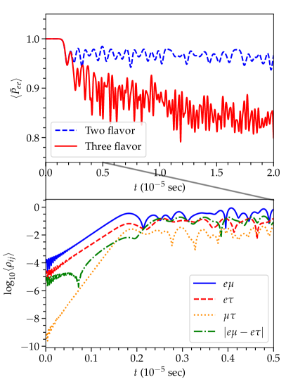
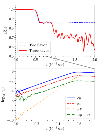
Figure 2: Left: Angle averaged ratio between the initial and final content of $\nu_{e}$ for Case I (see Eqs. 6a and 6b) as a function of time for $\mu=\lambda=10^{5}$ km¹ (blue dashed line for the two flavor approximation and red solid line for the three flavor case). In the inset on the bottom, the temporal evolution of the absolute values of the angle averaged off-diagonal elements of $3\times 3$ density matrix is shown. Right: Same as the left panels, but for $\mu=10^{4}$ km^-1. In both cases, the growth of $|\rho_{e\mu}-\rho_{e\tau}|$ in three flavors is responsible for the difference with respect to the two flavor case. The case with the smaller value of $\mu$ displays a growth rate for the off-diagonal elements that is smaller as expected from the linear stability analysis; however, the total conversion rate is larger (note the different ranges on the $y$-axis of the top panels).

The reason for the difference between two and three flavor evolution can be understood by looking at the off-diagonal elements of the density matrices. The inset on the bottom of Fig. 2 shows the angle averaged evolution of the absolute values of $|\rho_{e\mu}|$ and $|\rho_{e\tau}|$. They are almost identical in the linear regime where the growth of these quantities is exponential. In the two flavor approximation, the growth rate of the absolute value of the off-diagonal element is the same as $|\rho_{e\mu}|$ and $|\rho_{e\tau}|$ in the linear regime, and $|\rho_{e\mu}-\rho_{e\tau}|=0$. However, in three flavors, Fig. 2 shows that $|\rho_{e\mu}-\rho_{e\tau}|$ and $|\rho_{\mu\tau}|$ grow exponentially, breaking the symmetry between $\nu_{\mu}$ and $\nu_{\tau}$ sectors. These findings highlight that the fast flavor evolution is intrinsically different in three flavors from the two flavor case. The stark difference between the two flavor and three flavor cases was not reported in Ref. Chakraborty and Chakraborty (2020) since it can be captured by the linear stability analysis only on a sub-leading level due to the growth of $|\rho_{e\mu}-\rho_{e\tau}|$, while it becomes very evident in the non-linear regime.

Our findings highlight that the fast flavor evolution of two and three flavor systems can be significantly different even in the case of trivial initial angular distributions for the non-electron type neutrinos, differently from what pointed out in Ref. Capozzi et al. (2020). It should be noted that, although we have solved the system of equations including the matter term, our results are not sensitive to the exact value of the matter potential, as shown in Appendix B.

III.2 Case I: Dependence of the flavor conversion physics on the vacuum mixing parameters

The dramatic difference between the neutrino conversion physics in two and three flavors naturally raises questions on the sensitivity of the three flavor evolution to the specific choice of the mixing parameters. To this purpose, in Fig. 3, we explore the dependence of $\langle\widetilde{P}_{ee}\rangle$ on $\theta_{12}$ (left) and $\theta_{23}$ (right). The temporal evolution of the three flavor system is fairly independent on the vacuum mixing parameters. However, minor quantitative differences due to the exact value of $\theta_{12}$ are visible in the left panel of Fig. 3. Irrespective of the value of $\theta_{12}$, rapid oscillations develop over time and the survival probability reaches smaller values than the one in the two flavor case shown in Fig. 2. The dependence of $\langle\widetilde{P}_{ee}\rangle$ on $\theta_{23}$ (right panel of Fig. 3) is negligible, as expected Akhmedov et al. (2004); Fogli et al. (2009).

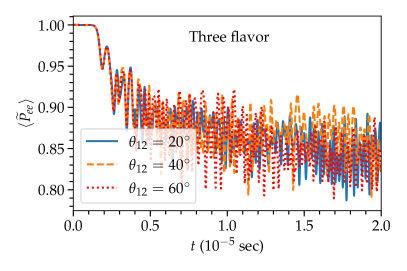
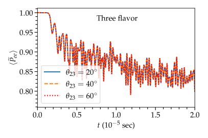
Figure 3: Temporal evolution of $\langle\widetilde{P}_{ee}\rangle$ for Case I for three different values of $\theta_{12}$ (left) and $\theta_{23}$ (right), respectively. A small quantitative dependence of $\langle\tilde{P}_{ee}\rangle$ on $\theta_{12}$ is visible, although the qualitative behavior is unchanged. Absolutely no dependence on $\theta_{23}$ is evident instead.

We have also verified that our results are qualitatively insensitive to all other vacuum mixing parameters, including the $\mathcal{CP}$-phase $\delta$ (results not shown here). The role of the vacuum mixing angles is to provide seeds for the non-linear growth. The qualitative features of the system are, however, independent on the seeds. In addition, these findings confirm the high degree of numerical accuracy of our calculations.

III.3 Case II: Crossings in the $\mu$ and $\tau$ sectors

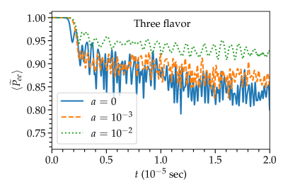
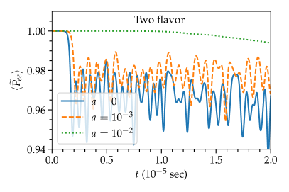
Figure 4: Left: Temporal evolution of $\langle\widetilde{P}_{ee}\rangle$ for various values of the parameter $a$ (see Eq. 8b). The high frequency modulations of $\langle\widetilde{P}_{ee}\rangle$ vanish as the magnitude of the nELN crossing exceeds a certain threshold (i.e., $a$ grows) and the three-flavor enhancement of conversions disappears. Right: The same as the left panel, but for the two flavor case. Also in the presence of nELN crossings, the two flavor case displays a different flavor outcome than the three flavor one.

As discussed in Refs. Capozzi et al. (2021, 2020), nELN crossings can occur in core-collapse supernovae and, in principle, can trigger additional flavor mixing. We explore the impact of $\mu$ neutrino lepton number crossings by setting up the system with initial conditions defined by Eqs. 6a, 6b, 8a, and 8b.

Figure 4 shows the angle averaged ratio between the initial and final content of $\nu_{e}$ for $a=0$, $10^{-3}$, and $10^{-2}$ in three (two) flavors on the left (right) panel. For small values of $a$, we do not see any substantial difference with respect to the $a=0$ case; however, for $a=10^{-2}$, the symmetry between non-electron neutrinos and antineutrinos is sufficiently broken. This leads to a disappearance of the enhancement of the flavor mixing caused by three flavor effects (see also Fig. 2 for comparison). Also in the presence of nELN crossings, the two flavor case displays a different flavor outcome than the three flavor one. The scenario with large $a$ ($a=10^{-2}$) captures the kind of effect also discussed in Ref. Capozzi et al. (2020) due to different angular distributions for the non-electron type neutrinos, in spite of the differences being much smaller in magnitude compared to those considered in Ref. Capozzi et al. (2020).

Our findings clearly show that nELN crossings, if much smaller in magnitude than the ELN one, negligibly affect the three flavor evolution. Due to the overwhelming excess of electrons over muons in supernovae as well as neutron star mergers, the difference between $\nu_{\mu}$ and $\bar{\nu}_{\mu}$ is bound to be far less substantial than the one between $\nu_{e}$ and $\bar{\nu}_{e}$ Bollig et al. (2017); Capozzi et al. (2021); hence, one should realistically expect scenarios similar to the ones discussed for small values of $a$.

It should be noted that the two flavor calculation in Ref. Capozzi et al. (2020) is performed by adopting an initial ensemble of $\nu_{e}$ and $\bar{\nu}_{e}$ only, while the three flavor calculation includes non-trivial initial angular distributions for the non-electron flavors Chakraborty and Chakraborty . This approach is not consistent since it is equivalent to consider the evolution of two systems with a different number of particles at $t=0$. In addition, it effectively changes the self-interaction potential strength and obfuscates the effect caused by the three flavor evolution due to the inherent differences determined by the non-trivial initial angular distributions of the non-electron type neutrinos. In the light of these differences, a direct comparison of our findings with the ones of Ref. Capozzi et al. (2020) is not possible.

IV The effect of collisions

The flavor evolution in the presence of matter is not only affected by the matter effect, but also by collisions Shalgar and Tamborra (2021b); Martin et al. (2021); Capozzi et al. (2019). In particular, contrary to conventional wisdom, collisions can lead to an enhancement of flavor conversions in certain circumstances Shalgar and Tamborra (2021b). Following Ref. Shalgar and Tamborra (2021b), we investigate whether collisions lead to an enhancement of flavor conversion in the three flavor framework.

We follow the same formalism as the one proposed in Ref. Shalgar and Tamborra (2021b) and modify Eq. 1 to include direction changing collisions:

$$\frac{d\rho(\cos\theta)}{dt}= - \int_{-1}^{1}\mathcal{C}_{\textrm{loss}}\rho(\cos\theta)d\cos\theta^{\prime}$$

$$+ \int_{-1}^{1}\mathcal{C}_{\textrm{gain}}\rho(\cos\theta^{\prime})d\cos\theta^{\prime}$$

$$- i[H(\cos\theta),\rho(\cos\theta)]\ ,$$

$$\frac{d\bar{\rho}(\cos\theta)}{dt}= - \int_{-1}^{1}\bar{\mathcal{C}}_{\textrm{loss}}\bar{\rho}(\cos\theta)d\cos\theta^{\prime}$$ (10)

$$+ \int_{-1}^{1}\bar{\mathcal{C}}_{\textrm{gain}}\bar{\rho}(\cos\theta^{\prime})d\cos\theta^{\prime}$$

$$- i[\bar{H}(\cos\theta),\rho(\cos\theta)]\ ,$$

where we assume that that $\mathcal{C}_{\textrm{loss}}=\mathcal{C}_{\textrm{gain}}=\bar{\mathcal{C}}_{\textrm{loss}}=\bar{\mathcal{C}}_{\textrm{gain}}$, implying particle number conservation as well as the same cross-section for neutrinos and antineutrinos. The inverse of the mean free path of the neutrinos can be expressed in terms of the collision terms by $\mathcal{C}=2\mathcal{C}_{\textrm{loss}}=2\mathcal{C}_{\textrm{gain}}=1$ km^-1 (see Appendix A for details on the numerical convergence).

As displayed in Fig. 5, obtained by relying on the initial conditions of Case I, the inclusion of collisions leads to an additional enhancement of flavor conversions on top of the one due to three flavor effects. This confirms the findings of Ref. Shalgar and Tamborra (2021b) and it is due to the fact that collisions redistribute the flavor content across angular bins creating more favorable conditions for flavor mixing.

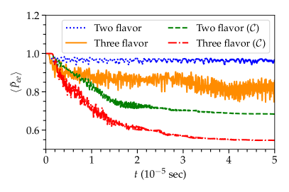
Figure 5: Temporal evolution of of $\langle\widetilde{P}_{ee}\rangle$ for the two and three flavor scenarios, with and without collisions. Collisions have the effect of further enhancing flavor mixing in two and three flavors.

V Conclusions and outlook

The consequences on flavor mixing of fast pairwise flavor conversion remain to be understood. In this paper, we compare the flavor outcome within the usually adopted two flavor approximation to the one resulting from the full three flavor case.

The two flavor approximation leads to differences with respect to the three flavor case already in the linear regime and such differences become amplified in the non-linear regime. The exponential growth of $|\rho_{e\mu}-\rho_{e\tau}|$ in three flavors (which remains zero in the two flavor approximation by definition) leads to a symmetry breaking between the $\nu_{\mu}$ and $\nu_{\tau}$ sectors that strongly affects the flavor conversion physics in the non-linear regime. This is a crucial difference at the essence of fast flavor mixing which was not pointed out in Refs. Capozzi et al. (2020).

The most vital component that leads to the failure of the two flavor approximation in fast flavor conversions is the nearly identical growth rate of $|\rho_{e\mu}|$ and $|\rho_{e\tau}|$; the latter is, however, seeded by a slightly different initial perturbation due to the vacuum Hamiltonian in three flavors.

Recent work has pointed out that the inclusion of muons in hydrodynamical simulations can lead to differences between the distributions of the non-electron flavors and induce crossings in the muon neutrino lepton number distributions Bollig et al. (2017); Capozzi et al. (2021). Although our findings are in qualitative agreement with the ones of Ref. Capozzi et al. (2020), this work shows that crossings in the angular distributions of non-electron type neutrinos are not crucial to appreciate an enhancement of flavor mixing in the full three flavor scenario. Notably, we find more extreme effects for smaller crossings in the non-electron flavors Bollig et al. (2017); Capozzi et al. (2021) on the flavor conversion probability, which have not been considered in Ref. Capozzi et al. (2020). Finally, the enhancement of flavor mixing in three flavors is further exacerbated by collisions.

In conclusions, it is vital to our understanding of the neutrino flavor evolution in any astrophysical system to include all three neutrino flavors. Our findings reinforce the limitations of the linear stability analysis as the conditions leading to the growth of flavor instabilities may seem identical for some components of the density matrix in two and three flavor systems; however the flavor conversion physics is inherently different in the non-linear regime.

Appendix A Numerical convergence of the results

The numerical results presented in this paper were obtained by carrying out simulations obtained by discretizing over the angular bins and numerically evolving Eqs. 1 for each angular bin. In order to do so, we rely on the Boost implementation of the eighth order Runge-Kutta-Fehlberg method with an adaptive step-size Boost (2019). To avoid any numerical error, we perform the numerical simulations with extremely tight absolute and relative tolerances of $10^{-16}$ and $10^{-12}$, respectively.

In addition, we have ensured that the number of angular bins is sufficient to reach convergence by solving Eqs. 1 with a different number of angular bins. For all the configurations considered in this paper, 5,000 angle bins have been tested to be sufficient to achieve convergence over the time scales of interest. An example is reported in Fig. 6, where the temporal evolution of $\langle\widetilde{P}_{ee}\rangle$ for Case I is shown for three different for 2,500, 5,000, and 10,000 angular bins.

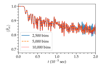
Figure 6: Temporal evolution of $\langle\widetilde{P}_{ee}\rangle$ for Case I for 2,500, 5,000, and 10,000 angle bins. $\langle\widetilde{P}_{ee}\rangle$ does not depend on the number of angular bins until $t=1.5\times 10^{-5}$ s, after that the results for 2,500 and 5,000 angular bins slightly diverge from each other. However, a comparison between the results obtained by employing 5,000 and 10,000 angular bins shows that 5,000 angle bins are sufficient to achieve convergence.

It should be noted that the number of angle bins required to achieve numerical convergence depends on the timescale over which the equations of motion are evolved. As $t$ increases, the angular distributions acquire structures on smaller scale. Consequently, for a given system configuration, the number of angular bins required for convergence increases as the time over which the system is evolved increases. This can be clearly seen in Fig. 6. The numerical results for 2,500 and 5,000 angle bins are identical up to $\simeq 1.5\times 10^{-5}$ s, after which they start deviating from each other. However, the employment of 5,000 angle bins guarantees convergence; in fact the evolution of $\langle\widetilde{P}_{ee}\rangle$ is identical to the one obtained by using 10,000 angular bins.

The inclusion of collisions smoothes out some of the angular structure and the number of angle bins required for a system with collisions is smaller than the one without collisions, as discussed in Ref. Shalgar and Tamborra (2021b); in our case, 1,000 angular bins were enough to guarantee numerically convergent results (related plots not shown here).

Appendix B Matter effects

In the two flavor approximation, the matter term has the effect of reducing the effective mixing angle while keeping the effective vacuum frequency unchanged Esteban-Pretel et al. (2008). It is thus possible to take into account the effect of the matter term by using a small effective mixing angle and keeping the vacuum frequency unchanged. However, it is not obvious whether this strategy can work in the three flavor approximation. To this purpose we set the initial conditions for the neutrino ensemble as in Case I and consider two different values of the matter potential, $\lambda=\mu$ and $\mu/100$.

Figure 7 shows the temporal evolution of $\langle\widetilde{P}_{ee}\rangle$ in two and three flavors for different values of $\lambda$. We can see that, although the features on a small time scale are affected by the matter term, the trend is unaffected by the matter term on a larger time-scale.

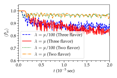
Figure 7: Temporal evolution of $\langle\widetilde{P}_{ee}\rangle$ in two and three flavors with $\mu=10^{5}$ km-1 and $\lambda=\mu$ and $\mu/100$. The blue dashed line shows the temporal evolution in the case of a matter potential that is smaller than the one expected in astrophysical scenarios, while the solid red line shows the flavor evolution for $\lambda=\mu$; the kind of matter potential expected in a realistic astrophysical system. The exact value of $\lambda$ does not affect the final flavor outcome drastically, but affects the onset of flavor conversions.

References

- Mikheev and Smirnov (1986) Stanislav P. Mikheev and Alexei Yu. Smirnov, “Neutrino Oscillations in a Variable Density Medium and Neutrino Bursts Due to the Gravitational Collapse of Stars,” Sov. Phys. JETP 64, 4–7 (1986), [,311(1986)], arXiv:0706.0454 [hep-ph] .
- Mikheyev and Smirnov (1985) Stanislav P. Mikheyev and Alexei Yu. Smirnov, “Resonance enhancement of oscillations in matter and solar neutrino spectroscopy,” Yadernaya Fizika 42, 1441–1448 (1985).
- Wolfenstein (1978) Lincoln Wolfenstein, “Neutrino oscillations in matter,” Phys. Rev. D 17, 2369–2374 (1978).
- Pantaleone (1992) James T. Pantaleone, “Neutrino oscillations at high densities,” Phys. Lett. B 287, 128–132 (1992).
- Sigl and Raffelt (1993) Günther Sigl and Georg G. Raffelt, “General kinetic description of relativistic mixed neutrinos,” Nucl. Phys. B 406, 423–451 (1993).
- Sawyer (2005) Raymond F. Sawyer, “Speed-up of neutrino transformations in a supernova environment,” Phys. Rev. D 72, 045003 (2005), arXiv:hep-ph/0503013 .
- Sawyer (2009) Raymond F. Sawyer, “The multi-angle instability in dense neutrino systems,” Phys. Rev. D 79, 105003 (2009), arXiv:0803.4319 [astro-ph] .
- Sawyer (2016) Raymond F. Sawyer, “Neutrino cloud instabilities just above the neutrino sphere of a supernova,” Phys. Rev. Lett. 116, 081101 (2016), arXiv:1509.03323 [astro-ph.HE] .
- Chakraborty et al. (2016a) Sovan Chakraborty, Rasmus Hansen, Ignacio Izaguirre, and Georg G. Raffelt, “Collective neutrino flavor conversion: Recent developments,” Nucl. Phys. B 908, 366–381 (2016a), arXiv:1602.02766 [hep-ph] .
- Chakraborty et al. (2016b) Sovan Chakraborty, Rasmus Sloth Hansen, Ignacio Izaguirre, and Georg G. Raffelt, “Self-induced neutrino flavor conversion without flavor mixing,” JCAP 03, 042 (2016b), arXiv:1602.00698 [hep-ph] .
- Tamborra and Shalgar (2021, in press) Irene Tamborra and Shashank Shalgar, “New Developments in Flavor Evolution of a Dense Neutrino Gas,” Ann. Rev. Nucl. Part. Sci. 71 (2021, in press), arXiv:2011.01948 [astro-ph.HE] .
- Izaguirre et al. (2017) Ignacio Izaguirre, Georg G. Raffelt, and Irene Tamborra, “Fast Pairwise Conversion of Supernova Neutrinos: A Dispersion-Relation Approach,” Phys. Rev. Lett. 118, 021101 (2017), arXiv:1610.01612 [hep-ph] .
- Shalgar and Tamborra (2021a) Shashank Shalgar and Irene Tamborra, “Dispelling a myth on dense neutrino media: fast pairwise conversions depend on energy,” JCAP 01, 014 (2021a), arXiv:2007.07926 [astro-ph.HE] .
- Xiong et al. (2020) Zewei Xiong, Andre Sieverding, Manibrata Sen, and Yong-Zhong Qian, “Potential Impact of Fast Flavor Oscillations on Neutrino-driven Winds and Their Nucleosynthesis,” Astrophys. J. 900, 144 (2020), arXiv:2006.11414 [astro-ph.HE] .
- Wu et al. (2017) Meng-Ru Wu, Irene Tamborra, Oliver Just, and Hans-Thomas Janka, “Imprints of neutrino-pair flavor conversions on nucleosynthesis in ejecta from neutron-star merger remnants,” Phys. Rev. D 96, 123015 (2017), arXiv:1711.00477 [astro-ph.HE] .
- George et al. (2020) Manu George, Meng-Ru Wu, Irene Tamborra, Ricard Ardevol-Pulpillo, and Hans-Thomas Janka, “Fast neutrino flavor conversion, ejecta properties, and nucleosynthesis in newly-formed hypermassive remnants of neutron-star mergers,” Phys. Rev. D in press (2020), arXiv:2009.04046 [astro-ph.HE] .
- Tamborra et al. (2017) Irene Tamborra, Lorenz Hüdepohl, Georg G. Raffelt, and Hans-Thomas Janka, “Flavor-dependent neutrino angular distribution in core-collapse supernovae,” Astrophys. J. 839, 132 (2017), arXiv:1702.00060 [astro-ph.HE] .
- Shalgar and Tamborra (2019) Shashank Shalgar and Irene Tamborra, “On the Occurrence of Crossings Between the Angular Distributions of Electron Neutrinos and Antineutrinos in the Supernova Core,” Astrophys. J. 883, 80 (2019), arXiv:1904.07236 [astro-ph.HE] .
- Abbar et al. (2019) Sajad Abbar, Huaiyu Duan, Kohsuke Sumiyoshi, Tomoya Takiwaki, and Maria Cristina Volpe, “On the occurrence of fast neutrino flavor conversions in multidimensional supernova models,” Phys. Rev. D100, 043004 (2019), arXiv:1812.06883 [astro-ph.HE] .
- Delfan Azari et al. (2019) Milad Delfan Azari, Shoichi Yamada, Taiki Morinaga, Wakana Iwakami, Hirotada Okawa, Hiroki Nagakura, and Kohsuke Sumiyoshi, “Linear Analysis of Fast-Pairwise Collective Neutrino Oscillations in Core-Collapse Supernovae based on the Results of Boltzmann Simulations,” Phys. Rev. D99, 103011 (2019), arXiv:1902.07467 [astro-ph.HE] .
- Delfan Azari et al. (2020) Milad Delfan Azari, Shoichi Yamada, Taiki Morinaga, Hiroki Nagakura, Shun Furusawa, Akira Harada, Hirotada Okawa, Wakana Iwakami, and Kohsuke Sumiyoshi, “Fast collective neutrino oscillations inside the neutrino sphere in core-collapse supernovae,” Phys. Rev. D 101, 023018 (2020), arXiv:1910.06176 [astro-ph.HE] .
- Glas et al. (2020) Robert Glas, Hans-Thomas Janka, Francesco Capozzi, Manibrata Sen, Basudeb Dasgupta, Alessandro Mirizzi, and Günter Sigl, “Fast Neutrino Flavor Instability in the Neutron-star Convection Layer of Three-dimensional Supernova Models,” Phys. Rev. D 101, 063001 (2020), arXiv:1912.00274 [astro-ph.HE] .
- Abbar et al. (2020) Sajad Abbar, Huaiyu Duan, Kohsuke Sumiyoshi, Tomoya Takiwaki, and Maria Cristina Volpe, “Fast Neutrino Flavor Conversion Modes in Multidimensional Core-collapse Supernova Models: the Role of the Asymmetric Neutrino Distributions,” Phys. Rev. D 101, 043016 (2020), arXiv:1911.01983 [astro-ph.HE] .
- Nagakura et al. (2019) Hiroki Nagakura, Taiki Morinaga, Chinami Kato, and Shoichi Yamada, “Fast-pairwise Collective Neutrino Oscillations Associated with Asymmetric Neutrino Emissions in Core-collapse Supernovae,” Astrophys. J. 886, 139 (2019), arXiv:1910.04288 [astro-ph.HE] .
- Morinaga et al. (2020) Taiki Morinaga, Hiroki Nagakura, Chinami Kato, and Shoichi Yamada, “Fast neutrino-flavor conversion in the preshock region of core-collapse supernovae,” Physical Review Research 2, 012046 (2020), arXiv:1909.13131 [astro-ph.HE] .
- Capozzi et al. (2021) Francesco Capozzi, Sajad Abbar, Robert Bollig, and Hans-Thomas Janka, “Fast neutrino flavor conversions in one-dimensional core-collapse supernova models with and without muon creation,” Phys. Rev. D 103, 063013 (2021), arXiv:2012.08525 [astro-ph.HE] .
- Abbar et al. (2021) Sajad Abbar, Francesco Capozzi, Robert Glas, H. Thomas Janka, and Irene Tamborra, “On the characteristics of fast neutrino flavor instabilities in three-dimensional core-collapse supernova models,” Phys. Rev. D 103, 063033 (2021), arXiv:2012.06594 [astro-ph.HE] .
- Duan et al. (2006a) Huaiyu Duan, George M. Fuller, and Yong-Zhong Qian, “Collective neutrino flavor transformation in supernovae,” Phys. Rev. D 74, 123004 (2006a), arXiv:astro-ph/0511275 [astro-ph] .
- Duan et al. (2006b) Huaiyu Duan, George M. Fuller, John Carlson, and Yong-Zhong Qian, “Simulation of Coherent Non-Linear Neutrino Flavor Transformation in the Supernova Environment. 1. Correlated Neutrino Trajectories,” Phys. Rev. D74, 105014 (2006b), arXiv:astro-ph/0606616 [astro-ph] .
- Duan et al. (2006c) Huaiyu Duan, George M. Fuller, John Carlson, and Yong-Zhong Qian, “Coherent Development of Neutrino Flavor in the Supernova Environment,” Phys. Rev. Lett. 97, 241101 (2006c), arXiv:astro-ph/0608050 [astro-ph] .
- Duan et al. (2007) Huaiyu Duan, George M. Fuller, J. Carlson, and Yong-Zhong Qian, “Neutrino Mass Hierarchy and Stepwise Spectral Swapping of Supernova Neutrino Flavors,” Phys. Rev. Lett. 99, 241802 (2007), arXiv:0707.0290 [astro-ph] .
- Duan et al. (2010) Huaiyu Duan, George M. Fuller, and Yong-Zhong Qian, “Collective Neutrino Oscillations,” Ann. Rev. Nucl. Part. Sci. 60, 569–594 (2010), arXiv:1001.2799 [hep-ph] .
- Fogli et al. (2009) Gianluigi Fogli, Eligio Lisi, Antonio Marrone, and Irene Tamborra, “Supernova neutrino three-flavor evolution with dominant collective effects,” JCAP 04, 030 (2009), arXiv:0812.3031 [hep-ph] .
- Dasgupta et al. (2010a) Basudeb Dasgupta, Alessandro Mirizzi, Irene Tamborra, and Ricard Tomas, “Neutrino mass hierarchy and three-flavor spectral splits of supernova neutrinos,” Phys. Rev. D 81, 093008 (2010a), arXiv:1002.2943 [hep-ph] .
- Dasgupta et al. (2010b) Basudeb Dasgupta, Georg G. Raffelt, and Irene Tamborra, “Triggering collective oscillations by three-flavor effects,” Phys. Rev. D 81, 073004 (2010b), arXiv:1001.5396 [hep-ph] .
- Dasgupta and Dighe (2008) Basudeb Dasgupta and Amol Dighe, “Collective three-flavor oscillations of supernova neutrinos,” Phys. Rev. D 77, 113002 (2008), arXiv:0712.3798 [hep-ph] .
- Dasgupta et al. (2008) Basudeb Dasgupta, Amol Dighe, Alessandro Mirizzi, and Georg G. Raffelt, “Spectral split in prompt supernova neutrino burst: Analytic three-flavor treatment,” Phys. Rev. D 77, 113007 (2008), arXiv:0801.1660 [hep-ph] .
- Friedland (2010) Alexander Friedland, “Self-refraction of supernova neutrinos: mixed spectra and three-flavor instabilities,” Phys. Rev. Lett. 104, 191102 (2010), arXiv:1001.0996 [hep-ph] .
- Bollig et al. (2017) R. Bollig, Hans-Thomas Janka, A. Lohs, G. Martínez-Pinedo, C. J. Horowitz, and T. Melson, “Muon Creation in Supernova Matter Facilitates Neutrino-driven Explosions,” Phys. Rev. Lett. 119, 242702 (2017), arXiv:1706.04630 [astro-ph.HE] .
- Airen et al. (2018) Sagar Airen, Francesco Capozzi, Sovan Chakraborty, Basudeb Dasgupta, Georg G. Raffelt, and Tobias Stirner, “Normal-mode Analysis for Collective Neutrino Oscillations,” JCAP 12, 019 (2018), arXiv:1809.09137 [hep-ph] .
- Chakraborty and Chakraborty (2020) Madhurima Chakraborty and Sovan Chakraborty, “Three flavor neutrino conversions in supernovae: slow fast instabilities,” JCAP 01, 005 (2020), arXiv:1909.10420 [hep-ph] .
- Capozzi et al. (2020) Francesco Capozzi, Madhurima Chakraborty, Sovan Chakraborty, and Manibrata Sen, “Fast flavor conversions in supernovae: the rise of mu-tau neutrinos,” Phys. Rev. Lett. 125, 251801 (2020), arXiv:2005.14204 [hep-ph] .
- Zyla et al. (2020) P.A. Zyla et al. (Particle Data Group), “Review of Particle Physics,” PTEP 2020, 083C01 (2020).
- Esteban-Pretel et al. (2008) Andreu Esteban-Pretel, Alessandro Mirizzi, Sergio Pastor, Ricard Tomàs, Georg G. Raffelt, Pasquale D. Serpico, and Günther Sigl, “Role of dense matter in collective supernova neutrino transformations,” Phys. Rev. D 78, 085012 (2008), arXiv:0807.0659 [astro-ph] .
- Akhmedov et al. (2004) Evgeny K. Akhmedov, Robert Johansson, Manfred Lindner, Tommy Ohlsson, and Thomas Schwetz, “Series expansions for three flavor neutrino oscillation probabilities in matter,” JHEP 04, 078 (2004), arXiv:hep-ph/0402175 .
- (46) Madhurima Chakraborty and Sovan Chakraborty, “Private Communication.” .
- Shalgar and Tamborra (2021b) Shashank Shalgar and Irene Tamborra, “A change of direction in pairwise neutrino conversion physics: The effect of collisions,” Phys. Rev. D 103, 063002 (2021b), arXiv:2011.00004 [astro-ph.HE] .
- Martin et al. (2021) Joshua D. Martin, John Carlson, Vincenzo Cirigliano, and Huaiyu Duan, “Fast flavor oscillations in dense neutrino media with collisions,” (2021), arXiv:2101.01278 [hep-ph] .
- Capozzi et al. (2019) Francesco Capozzi, Basudeb Dasgupta, Alessandro Mirizzi, Manibrata Sen, and Günter Sigl, “Collisional triggering of fast flavor conversions of supernova neutrinos,” Phys. Rev. Lett. 122, 091101 (2019), arXiv:1808.06618 [hep-ph] .
- Boost (2019) Boost, “Boost C++ Libraries,” http://www.boost.org/ (2019).