Implications of new evidence for lepton-universality violation in $b\to s\ell^{+}\ell^{-}$ decays

Abstract

Motivated by renewed evidence for new physics in $b\to s\ell\ell$ transitions in the form of LHCb’s new measurements of theoretically clean lepton-universality ratios and the purely leptonic $B_{s}\to\mu^{+}\mu^{-}$ decay, we quantify the combined level of discrepancy with the Standard Model and fit values of short-distance Wilson coefficients. A combination of the clean observables $R_{K}$, $R_{K^{*}}$, and $B_{s}\to\mu\mu$ alone results in a discrepancy with the Standard Model at $4.0\sigma$, up from $3.5\sigma$ in 2017. One-parameter scenarios with purely left-handed or with purely axial coupling to muons fit the data well and result in a $\sim 5\sigma$ pull from the Standard Model. In a two-parameter fit of new-physics contributions with both vector and axial-vector couplings to muons the allowed region is much more restricted than in 2017, principally due to the much more precise result on $B_{s}\to\mu^{+}\mu^{-}$, which probes the axial coupling to muons. Including angular observables data restricts the allowed region further. A by-product of our analysis is an updated average of $\text{BR}(B_{s}\to\mu^{+}\mu^{-})=(2.8\pm 0.3)\times 10^{-9}$.

I Introduction

Flavor physics played a central role in the development of the Standard Model (SM) and could well spearhead the discovery of new physics (NP) beyond the SM (BSM). In fact, although the vast majority of particle-physics data is consistent with the predictions of the SM, a conspicuous series of discrepancies has appeared in rare flavor-changing processes mediated by quark-level $b\to s\ell\ell$ transitions. These are suppressed by the “GIM mechanism” in the SM and are, therefore, potentially sensitive to very high-energy NP scales Buras (2020). A perennial question in this context is how to distinguish long-distance strong-interaction effects from genuine new physics. Several years ago, following LHCb’s first measurement of the lepton-universality violating ratio $R_{K^{*}}$, we demonstrated Geng et al. (2017) the power of using observables which are almost entirely free from hadronic uncertainties to provide a high-significance rejection of the SM, and its potential to narrow down the chiral structure of the BSM effect. In particular, we pointed out the importance of the $B_{s}\to\mu^{+}\mu^{-}$ decay and lepton-flavor-violating ratios of forward-backward asymmetries in lifting a degeneracy between axial and vectorial couplings to leptons. Motivated by LHCb’s updates to the ratio $R_{K}$ and of $\text{BR}(B_{s}\to\mu^{+}\mu^{-})$ we revisit this set of decays in the present work.

II Observables

The measurement of several rare $b\to s\ell\ell$ decays yields results in tension with the SM expectations implying the presence of new interactions breaking lepton universality (see Refs. Bifani et al. (2019); Buras (2020) for recent reviews). Among them stand out a subset of observables with theoretical uncertainties at or below the percent level Hiller and Kruger (2004); Beneke et al. (2018). Our main observables of interest comprise the lepton-universality ratios $R_{K}=\Gamma(B\to K\mu\mu)/\Gamma(B\to Kee)$ Hiller and Kruger (2004) and $R_{K^{*}}=\Gamma(B\to{K^{*}}\mu\mu)/\Gamma(B\to{K^{*}}ee)$, and the purely leptonic decay $B_{s}\to\mu^{+}\mu^{-}$.

In particular, the LHCb collaboration has just reported the most precise measurement of $R_{K}$ in the $q^{2}$-bin $[1.1,6]~{}{\rm GeV}^{2}$ using the full run 1 and 2 datasets Aaij et al. (2021a),

$$R_{K}=0.846^{+0.042+0.013}_{-0.039-0.012}\;,$$ (1)

where the first uncertainty is statistical and the second systematic. This result deviates from the SM predictions (see Table I in Ref. Geng et al. (2017)) 

$$R_{K}^{\rm SM}=1.0004^{+0.0008}_{-0.0007}\;,$$ (2)

with a significance of $3.1\sigma$. Compared to the first LHCb measurement reported in 2014 Aaij et al. (2014), the tension with respect to the SM has significantly increased.

At the same time, LHCb has published new results for the branching faction of $B_{s}\to\mu^{+}\mu^{-}$,

$${\rm BR}(B_{s}\to\mu^{+}\mu^{-})=(3.09^{+0.46+0.15}_{-0.43-0.11})\times 10^{-9},$$ (3)

obtained with the same full dataset Santimaria (2021) and also known to about 1% accuracy in the SM. This result, along with other recent measurements done by ATLAS Aaboud et al. (2019) and CMS Sirunyan et al. (2020), indicate a decay rate lower than the SM prediction. This set of key inputs is summarized in Table 1. In place of the asymmetric errors on $R_{K}$ and $R_{K^{*}}$ published by the experiments, we conservatively employ a symmetric error equal to the upper, larger error (combining statistical and systematic in quadrature), in line with the treatment in Ref. Geng et al. (2017).

Table 1: Key inputs used in this paper.

Observable	Value	Source	Reference
${\rm BR}(B_{s}\to\mu^{+}\mu^{-})$	$(2.8{}^{+0.8}_{-0.7})\times 10^{-9}$	ATLAS	Aaboud et al. (2019)
	$(2.9\pm 0.7\pm 0.2)\times 10^{-9}$	CMS	Sirunyan et al. (2020)
	$(3.09^{+0.46+0.15}_{-0.43-0.11})\times 10^{-9}$	LHCb update	Santimaria (2021)
	$(2.842\pm 0.333)\times 10^{-9}$	Our average	This work
	$(3.63\pm 0.13)\times 10^{-9}$	SM prediction	Beneke et al. (2019)
$R_{K}[1.1,6]$	$0.846\pm 0.044$	LHCb	Aaij et al. (2021a)
$R_{K}[1,6]$	$1.03\pm 0.28$	Belle	Abdesselam et al. (2019a)
$R_{K^{*}}[0.045,1.1]$	$0.660\pm 0.113$	LHCb	Aaij et al. (2017a)
$R_{K^{*}}[1.1,6]$	$0.685\pm 0.122$	LHCb	Aaij et al. (2017a)
$R_{K^{*}}[0.045,1.1]$	$0.52\pm 0.365$	Belle	Abdesselam et al. (2019b)
$R_{K^{*}}[1.1,6]$	$0.96\pm 0.463$	Belle	Abdesselam et al. (2019b)

In 2020 LHCb also reported a new measurement of the $CP$-averaged angular observables of the decay $B^{0}\to K^{*0}\mu^{+}\mu^{-}$ Aaij et al. (2020a) and of its isospin partner, $B^{+}\to K^{*+}\mu^{+}\mu^{-}$ Aaij et al. (2020b). The new data seems to confirm the previous measurements pointing to possible tensions with the SM D’Amico et al. (2017); Ciuchini et al. (2020); Munir Bhutta et al. (2020); Bečirević et al. (2020); Alasfar et al. (2020); Hurth et al. (2020); Bhom et al. (2020); Descotes-Genon et al. (2020); Biswas et al. (2020); Bordone et al. (2020); Coy et al. (2020); Bhattacharya et al. (2020); Arbey et al. (2019); Kowalska et al. (2019); Algueró et al. (2019a); Aebischer et al. (2020); Ciuchini et al. (2019); Alok et al. (2019); Algueró et al. (2019b); Kumar and London (2019); Datta et al. (2019). However, and contrary to the lepton-universality ratios and $B_{s}\to\mu\mu$, the SM predictions for the $B\to K^{*}\mu\mu$ angular observables suffer from significant hadronic uncertainties which hinder a clear interpretation of the discrepancies in terms of NP Beneke et al. (2001); Grinstein and Pirjol (2004); Egede et al. (2008); Khodjamirian et al. (2010); Beylich et al. (2011); Khodjamirian et al. (2013); Descotes-Genon et al. (2013); Jäger and Martin Camalich (2013); Horgan et al. (2014); Lyon and Zwicky (2014); Descotes-Genon et al. (2014); Jäger and Martin Camalich (2016); Bharucha et al. (2016); Ciuchini et al. (2016); Hiller and Nisandzic (2017); Chobanova et al. (2017); Bobeth et al. (2018); Aaij et al. (2017b); Gubernari et al. (2019).

In this work we combine the experimental data focusing on the clean observables as in Ref. Geng et al. (2017) and carry out global fits of the Wilson coefficients (or short-distance coefficients) of the low-energy $b\to s\ell\ell$ effective Lagrangian to the data. We find that the data on clean observables is at variance with the SM at a level of 4.0$\sigma$. We also find that one-parameter scenarios with purely left-handed or axial currents provide a good description of the data, excluding the SM point in each case at close to 5$\sigma$. As discussed abundantly in the literature, such new lepton-universality-violating (LUV) interactions can arise at tree or loop level from new mediators such as neutral vector bosons ($Z^{\prime}$) or leptoquarks (see Ref. Cerri et al. (2019) which includes a review of NP interpretations).

II.1 Combination of ${\rm BR}(B_{s}\to\mu^{+}\mu^{-}$) data

An important aspect to note is that the three measurements of $B_{s}\to\mu^{+}\mu^{-}$ cannot be naively averaged together, as a result of correlations with $B_{d}\to\mu^{+}\mu^{-}$. We therefore construct a two-dimensional joint likelihood from the published measurements Aaboud et al. (2019); Sirunyan et al. (2020); Santimaria (2021). In doing so, we assume a correlation coefficient of $-0.5$ for ATLAS, which reproduces the results reported in Ref. Aaboud et al. (2019), and neglect correlations in the LHCb measurement. The resulting combination is represented in Fig. 1. Profiling over $\text{BR}(B_{d}\to\mu^{+}\mu^{-})$ results in

$$\text{BR}(B_{s}\to\mu^{+}\mu^{-}) = (2.8\pm 0.3)\times 10^{-9}$$ (4)

with $\chi^{2}_{\rm min}=3.72$ (5 d.o.f.).  As with the existing combination LHC (2020), the central value of the average is lower than the average of the three individual central values.

We combine the experimental measurements and the SM prediction of the $B_{s}\to\mu^{+}\mu^{-}$ branching fraction in the ratio

$$R=\frac{{\rm BR}(B_{s}^{0}\to\mu^{+}\mu^{-})_{\rm exp}}{{\rm BR}(B_{s}^{0}\to\mu^{+}\mu^{-})_{\rm SM}},$$ (5)

obtaining $R=0.78(9)$ by using the most up to date theoretical prediction of Ref. Beneke et al. (2018). We end this section by noting that only the recent LHCb result implements a newer (and larger by $\sim 6\%$) measurement of the ratio of hadronization fractions $f_{s}/f_{d}$. However, including the corresponding increase in the branching fractions of $B_{s}\to\mu^{+}\mu^{-}$ measured by ATLAS and CMS (keeping the correlation with $B_{d}\to\mu^{+}\mu^{-}$) leads to a very small increase (of about $\sim 3\%$) in the average in Eq. (4) that will be neglected in this work.

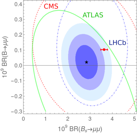
Figure 1: Our combination of measurements of $\text{BR}(B_{s,d}\to\mu^{+}\mu^{-}$) by ATLAS Aaboud et al. (2019), CMS Sirunyan et al. (2020), and LHCb Santimaria (2021), compared to the SM prediction (red square). Contours of the combination correspond to 1$\sigma$, 2$\sigma$ and 3$\sigma$, and those of each experiment to just 3$\sigma$.

III Theoretical approach

The low-energy effective Hamiltonian for semileptonic $b\rightarrow s\ell^{+}\ell^{-}$ processes at the scale $\mu\sim m_{b}$ in the SM is written as Buchalla et al. (1996)

$${\cal{H}}_{\rm eff}^{\rm SM}=\frac{4G_{F}}{\sqrt{2}}\sum_{p=u,c}\lambda_{ps}\left(C_{1}{\cal O}_{1}^{p}+C_{2}{\cal O}_{2}^{p}+\sum_{i=3}^{10}C_{i}{\cal O}_{i}\right),$$ (6)

where $G_{F}$ is the Fermi constant, and $\lambda_{ps}=V_{pb}V_{ps}^{*}$ is a combination of Cabibbo-Kobayashi-Maskawa (CKM) matrix elements with $p=u,c$. The short-distance contributions, stemming from scales above $\mu\sim m_{b}$, are matched to a set of Wilson coefficients $C_{i}$. The ${\cal O}_{1,2}^{p}$, ${\cal O}_{3-6}$ and ${\cal O}_{8}$ are the “current-current”, “QCD-penguin” and “chromomagnetic” operators, respectively. The explicit forms for these operators can be found in Ref. Buchalla et al. (1996). The remaining operators ${\cal O}_{7}$, ${\cal O}_{9}$, and ${\cal O}_{10}$ from electromagnetic penguin-, electroweak penguin-, and box-loop diagrams are defined as follows:

$$\qquad\qquad\qquad O_{7}=\frac{e}{16\pi^{2}}m_{b}(\bar{s}\sigma^{\mu\nu}P_{R}b)F_{\mu\nu},$$

$$O_{9}^{\ell}=\frac{e^{2}}{16\pi^{2}}(\bar{s}\gamma^{\mu}P_{L}b)(\bar{\ell}\gamma_{\mu}\ell),~{}~{}O_{10}^{\ell}=\frac{e^{2}}{16\pi^{2}}(\bar{s}\gamma^{\mu}P_{L}b)(\bar{\ell}\gamma_{\mu}\gamma_{5}\ell).$$

In the presence of NP, one has nine more operators, i.e., $O_{7}^{\prime}$ and $O_{9,10}^{\prime\ell}$, the opposite-quark-chirality counterparts of $O_{7}$ and $O_{9,10}^{\ell}$, plus four scalar and two tensor operators Alonso et al. (2014). However, if the NP effect enters in the couplings to muons, only ${\cal O}_{9}$ and ${\cal O}_{10}$ can explain the $R_{K^{(*)}}$ data Alonso et al. (2014). The tensor-operator contributions to $b\to s\ell\ell$ decays are suppressed if the NP scale is heavier than the electroweak scale. Other operators cannot induce LUV, or are tightly constrained by the $B_{q}\to\ell\ell$ decays. In the following analysis, we assume that all the Wilson coefficients are real and that the presence of NP only appears in the $b\to s\mu^{+}\mu^{-}$ sector. The last assumption is justified by the tension in the data in $b\to s\mu^{+}\mu^{-}$, in particular in BR($B_{s}\to\mu^{+}\mu^{-}$) discussed above.

For reliable predictions of observables, it is of vital importance to estimate theoretical uncertainties. They mainly stem from nonperturbative contributions including form factors $F(q^{2})$’s and “nonfactorizable” terms $h_{\lambda}(q^{2})$’s Beneke et al. (2001). At low $q^{2}$ the nonperturbative contributions can be addressed in the heavy quark and large-energy limits: they can be expanded as Jäger and Martin Camalich (2016),

$$F(q^{2})=F^{\infty}(q^{2})+a_{F}+b_{F}q^{2}/m_{B}^{2}+{\cal O}\left((q^{2}/m_{B}^{2})^{2}\right),$$

$$h_{\lambda}(q^{2})=h_{\lambda}^{\infty}(q^{2})+r_{\lambda}(q^{2}),$$ (8)

where $F^{\infty}(q^{2})$ and $h_{\lambda}^{\infty}(q^{2})$ can be calculated in light-cone sum rules Ball and Zwicky (2005); Khodjamirian et al. (2010) and within the QCD factorization approach Beneke et al. (2001), and the rest are power-correction terms. Among them, $r_{\lambda}(q^{2})$ is dominated by the long-distance charm contributions involving the “current-current” operators ${\cal O}_{1}^{c}$ and ${\cal O}_{2}^{c}$ Jäger and Martin Camalich (2016). We parametrize the charm loop contributions, $r_{\lambda}^{c}(q^{2})$, by

$$r_{\lambda}^{c}(q^{2})=A_{\lambda}+B_{\lambda}\frac{q^{2}}{4m_{c}^{2}},$$ (9)

where $A_{\lambda}$ and $B_{\lambda}$ are dimensionless constants. Therefore, the overall uncertainties at low $q^{2}$ arise from the leading-power terms, power corrections of form factors and charm loop contributions, characterized by 27 nuisance parameters. For more details and ranges of values taken for these, see Refs. Jäger and Martin Camalich (2016); Geng et al. (2017). In the high-$q^{2}$ region, form factors have been calculated in lattice QCD Horgan et al. (2014) whereas the nonfactorizable contribution can be computed with an operator product expansion Grinstein and Pirjol (2004); Beylich et al. (2011). We omit the analysis of this region as none of the LUV ratios have been measured there yet.

We use the frequentist statistical approach to quantify the compatibility between the experimental data and the theoretical predictions. We define the $\chi^{2}$ function as

$$\tilde{\chi}^{2}(\vec{C},~{}\vec{y})=\chi^{2}_{\rm exp}(\vec{C},~{}\vec{y})+\chi^{2}_{\rm th}(\vec{y}),$$ (10)

where $\chi^{2}_{\rm exp}(\vec{C},~{}\vec{y})$ includes the correlations reported by the experiments and $\chi^{2}_{\rm th}(\vec{y})$ is a theoretical component.

The theoretical predictions for the observables $O^{\rm th}$ are functions of Wilson coefficients $\vec{C}$ and nuisance hadronic parameters $\vec{y}$. We choose two models for $\chi^{2}_{\rm th}(\vec{y})$; one in which $y_{i}$ follows a normal distribution (that we call “Gaussian”) and another (that we call “$R$-fit”) where it is restricted to a range, see Ref. Jäger and Martin Camalich (2016), with a flat distribution. Here, we assume that these nuisance parameters are uncorrelated Jäger and Martin Camalich (2016).

In order to obtain best-fit values in a particular scenario, we can construct a profile $\chi^{2}$ depending only on certain Wilson coefficients

$$\chi^{2}(\vec{C})=\underset{\vec{y}}{\rm min}\,\tilde{\chi}^{2}(\vec{C},\vec{y}),$$ (11)

with the remaining Wilson coefficients set to their SM values. Here, $\chi^{2}$ is minimized by varying the nuisance parameters. In our statistical analysis, we adopt the widely used $p$-value and ${\rm Pull}_{\rm SM}$ to denote how well the experimental data can be described and how significant is the deviation from the SM. Results of fits are reported for $\delta C_{i}\equiv C_{i}-C_{I}^{\text{SM}}$.

Table 2: Best-fit values, $\chi_{\rm min}^{2}$, $p$-value, ${\rm Pull}_{\rm SM}$ and confidence intervals of the Wilson coefficients in the fits of the $R_{K}$, $R_{K^{*}}$, $B_{s}\to\mu\mu$ data only using Gaussian form $\chi^{2}_{\rm th}$. For the cases of single Wilson-coefficient fits, we show the $1\sigma$ and $3\sigma$ confidence intervals. In the $(\delta C_{9}^{\mu},\delta C_{10}^{\rm\mu})$ case, the $1\sigma$ interval of each Wilson coefficient is obtained by profiling over the other one to take into account their correlation.

Coefficient	Best fit	$\chi^{2}_{\rm min}$	$p$-value	${\rm Pull}_{\rm SM}$ [$\sigma$]	1$\sigma$ range	3$\sigma$ range	$\rho$
$\delta C_{9}^{\mu}$	$-0.82$	14.70 [6 d.o.f.]	0.02	4.08	$[-1.06,-0.60]$	$[-1.60,~{}-0.20]$	$\cdots$
$\delta C_{10}^{\mu}$	0.65	6.52   [6 d.o.f.]	0.37	4.98	$[0.52,0.80]$	$[0.25,1.11]$	$\cdots$
$\delta C_{L}^{\mu}$	$-0.40$	7.36 [6 d.o.f.]	0.29	4.89	$[-0.48,-0.31]$	$[-0.66,-0.15]$	$\cdots$
$(\delta C_{9}^{\mu},\delta C_{10}^{\rm\mu})$	$(-0.11,0.59)$	6.38  [5 d.o.f.]	0.27	4.62	$\delta C_{9}^{\mu}\in$ $[-0.41,~{}0.17]$	$\delta C_{10}^{\mu}\in$ $[0.38,~{}0.81]$	$0.762$
$(\delta C_{L}^{\mu},\delta C_{R}^{\rm\mu})$	$(-0.35,0.25)$				$\delta C_{L}^{\mu}\in[-0.45,-0.26]$	$\delta C_{R}^{\mu}\in[0.00,0.48]$	$0.406$

IV The theoretically clean fit

We first restrict ourselves to the analysis of the theoretically clean observables $R_{K}$, $R_{K^{*}}$ and $B_{s}\to\mu^{+}\mu^{-}$. The relevant data is shown in Table 1 and discussed above. We first assess the consistency of the dataset, which gives $\chi^{2}_{\rm min}=4.61$ ($8$ d.o.f.), corresponding to $p=0.80$, where $p$ denotes $p$-value. For the d.o.f. we count the 6 $B_{q}\to\mu^{+}\mu^{-}$ measurements separately and for $R_{K}$ we count the LHCb and Belle results as two separate measurements of the same observable, neglecting the small difference in the lower end of the bin.

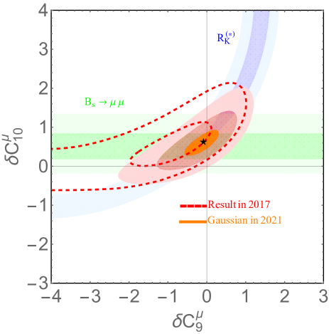
Figure 2: Contour plots at the $1\sigma$, $3\sigma$ and $5\sigma$ confidence levels in the $(\delta C_{9}^{\mu},\delta C_{10}^{\mu})$ plane for the Gaussian form of $\chi^{2}_{\rm th}$ (regions in light red and orange). We also show the $1\sigma$ and $3\sigma$ contours for the individual constraints ($R_{K^{(*)}}$ and $B_{s}\to\mu\mu$) and, for the same fit from 2017 Geng et al. (2017) (dashed in red).

Minimizing $\chi^{2}$ over all SM and theoretical nuisance parameters, one obtains $\chi_{\rm min,SM}^{2}=31.32$ ($\chi_{\rm min,SM}^{2}=30.54$) and $p_{\rm SM}=5.4\times 10^{-5}$ ($p_{\rm SM}=7.6\times 10^{-5}$) using the Gaussian ($R$-fit) form of the $\chi^{2}_{\rm th}$. We emphasize that the sole role of the minimization here is to implement the tiny theoretical uncertainties. In arriving at this $p$-value and in the rest of this paper, we treat our ${\rm BR}(B_{s}\to\mu^{+}\mu^{-})$ average as a single measurement, following common practice and in line with Ref. Geng et al. (2017). In other words, with 7 d.o.f. the clean data is at variance with the null hypothesis (Standard Model) at a level of $4.0\sigma$, up from $3.5\sigma$ in our previous work Geng et al. (2017). Were we to treat the 6 $B_{q}\to\mu^{+}\mu^{-}$ measurements as separate inputs, we would instead obtain $\chi^{2}_{\rm min,SM}=35.04$ and $p_{\rm SM}=3.5\sigma$ (12 d.o.f.); the reduction in significance is unsurprising given that we now include (nonanomalous) data on $b\to d\ell\ell$ transitions. We next fit one- and two-parameter BSM scenarios. Only $\delta C_{9}^{\mu}$ and $\delta C^{\mu}_{10}$ can describe a deficit in both $R_{K}$ and $R_{K^{*}}$ (Ref. Geng et al. (2017) and Fig. 1 there). Therefore we analyze the data in the clean observables by fitting only these two Wilson coefficients. Figure 2 shows the constraints imposed in the $(\delta C_{9}^{\mu},\delta C_{10}^{\mu})$ plane and using the Gaussian model for $\chi^{2}_{\rm th}$ (see below for the $R$-fit results). In Table 3 we also show the numerical results for this fit, as well as fits involving a single Wilson coefficient, for the Gaussian approach. We also fit the left- and right-handed combinations (related to the couplings to muons) of Wilson coefficients $\delta C_{L}^{\mu}=(\delta C_{9}^{\mu}-\delta C_{10}^{\mu})/2$ and $\delta C_{R}^{\mu}=(\delta C_{9}^{\mu}+\delta C_{10}^{\mu})/2$. We observe that one-parameter scenarios with purely left-handed coupling $\delta C_{L}^{\mu}$ or purely axial coupling $\delta C_{10}^{\mu}$ describe the data well ($p>10\%$). Compared to either scenario, the SM (identified as the $\delta C_{i}=0$ point) is excluded at a confidence level of close to $5\sigma$. On the other hand, and in contrast with our previous analysis from 2017 Geng et al. (2017), the pure-$C_{9}$ scenario is in tension with the data at $2.3\sigma$ although it still compares favorably with the data compared to the SM. Finally, as we will see below, using the $R$-fit version of $\chi^{2}_{\rm th}$ and increasing the theoretical uncertainties in the predictions of $B\to K^{(*)}\ell\ell$ only produce very small changes in the results of the fit to clean observables and do not change our conclusions.

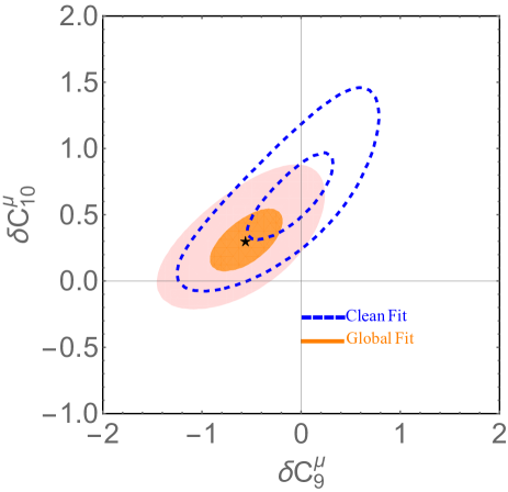
Figure 3: Contour plots at the $1\sigma$ and $3\sigma$ confidence level for the $(\delta C_{9}^{\mu},\delta C_{10}^{\mu})$ scenario. For comparison, we show the global fits with all observables for Gaussian (regions in light red and orange) and the corresponding clean fits of Fig. 2 (dashed lines in blue).

V The global fit

Table 3: The same as Table 2 but fitting to the $R_{K}$, $R_{K^{*}}$, $B_{s}\to\mu\mu$ and angular observables of $B\to K^{*}\mu\mu$ data.

Coefficient	Best fit	$\chi^{2}_{\rm min}$	$p$-value	${\rm Pull}_{\rm SM}$	1$\sigma$ range	3$\sigma$ range	$\rho$
$\delta C_{9}^{\mu}$	$-0.85$	106.32 [93 d.o.f.]	0.16	4.53	$[-1.06,-0.64]$	$[-1.50,-0.27]$	$\cdots$
$\delta C_{10}^{\mu}$	0.54	107.82 [93 d.o.f.]	0.14	4.37	[0.41, 0.67]	[0.16, 0.94]	$\cdots$
$\delta C_{L}^{\mu}$	$-0.39$	102.81 [93 d.o.f.]	0.23	4.91	$[-0.48,-0.31]$	$[-0.65,-0.15]$	$\cdots$
$(\delta C_{9}^{\mu},\delta C_{10}^{\mu})$	$(-0.56,0.30)$	102.36 [92 d.o.f.]	0.22	4.58	$\delta C_{9}^{\mu}\in$ $[-0.79,-0.31]$	$\delta C_{10}^{\mu}\in[0.15,0.49]$	$0.317$
$(\delta C_{L}^{\mu},\delta C_{R}^{\mu})$	$(-0.43,-0.12)$				$\delta C_{L}^{\mu}\in[-0.52,-0.33]$	$\delta C_{R}^{\mu}\in[-0.27,0.03]$	$0.364$

For the sake of completeness we also perform a global fit including all the measurements of angular observables reported by the LHCb, ATLAS, and CMS experiments in the low-$q^{2}$ region. As mentioned above, these observables are afflicted by larger theoretical uncertainties compared to LUV ratios and $B_{s}\to\mu\mu$. However, it is important to analyze how the conclusions change when including these data within a model-independent framework for the theoretical uncertainties such as ours.

More specifically, compared to our 2017 analysis Geng et al. (2017), we replace the $CP$-averaged angular observables for the $B^{0}\to K^{*0}\mu^{+}\mu^{-}$, the ratio $R$ for the $B_{s}\to\mu^{+}\mu^{-}$ decay, and $R_{K}$ in the bin $[1.1,~{}6.0]~{}{\rm GeV}^{2}$ with the latest measurements by the LHCb, CMS and ATLAS experiments Aaij et al. (2019, 2020a); Sirunyan et al. (2020); Aaboud et al. (2019); LHC (2020). In addition, we also include 32 new measurements of $F_{L}$, $P_{1}$, $P_{2}$, $P_{3}$, $P_{4}^{\prime}$, $P_{5}^{\prime}$, $P_{6}^{\prime}$ and $P_{8}^{\prime}$ in four low bins ($q^{2}\leq 6~{}{\rm GeV}^{2}$) for the $B^{+}\to K^{*+}\mu^{+}\mu^{-}$ decay Aaij et al. (2020b) as well as three Belle data $R_{K}$ and $R_{K^{*}}$ in Table 1. As a result the total number of data fitted becomes 94. 

In this fit strategy, we obtain a $\chi_{\rm min,SM}^{2}=126.88$ and $p_{\rm SM}=0.01$ with 94 d.o.f.. Compared to the global fit results in Ref. Geng et al. (2017), the updated fit results in Table 3 and Fig. 3 show that the confidence level of the exclusion of the SM point increases by $1.3\sigma$ for the $\delta C_{10}^{\mu}$ scenario and by $0.7\sigma$ for the $\delta C_{L}^{\mu}$ scenario, but only by $0.2\sigma$ and $0.4\sigma$ in the $\delta C_{9}^{\mu}$ and $(\delta C_{9}^{\mu},\delta C_{10}^{\mu})$ scenarios, respectively. Interestingly, these updated fits constrain better these Wilson coefficients and exclude positive $\delta C_{9}^{\mu}$ and negative $\delta C_{10}^{\mu}$ at more than the $3\sigma$ confidence level.

We also perform a four-dimensional global fit with the Gaussian $\chi^{2}_{\rm th}$ including $C_{9}^{\prime\mu}$ and $C_{10}^{\prime\mu}$. The resulting Wilson coefficients from the fit are,

$$\left(\begin{array}[]{c}\delta C_{9}^{\mu}\\ \delta C_{10}^{\mu}\\ C_{9}^{\prime\mu}\\ C_{10}^{\prime\mu}\end{array}\right)=\left(\begin{array}[]{c}-1.07\pm 0.29\\ 0.21\pm 0.14\\ 0.32\pm 0.21\\ -0.26\pm 0.14\end{array}\right),$$ (20)

with the correlation matrix,

$$\rho=\left(\begin{array}[]{cccc}1.000&0.529&-0.381&0.455\\ &1.000&0.010&0.263\\ &&1.000&0.153\\ &&&1.000\end{array}\right),$$ (25)

and where $\chi_{\rm min}^{2}=96.88$ for 90 d.o.f., corresponding to a $p$-value of 0.29 and a Pull${}_{\rm SM}=4.57$.

VI Impact of theoretical uncertainties

Finally, we briefly investigate the robustness of the fits with respect to the hadronic uncertainties. We do so by comparing the results obtained above with those obtained by using the $R$-fit model for $\chi^{2}_{\rm th}$, with nominal hadronic uncertainties in $B\to K^{(*)}\ell\ell$ or multiplied by a factor 2 and 3. The relevant results are shown in Tables 4, 5 and  6. In Fig. 4 we also show the new results in the $(\delta C_{9}^{\mu},~{}\delta C_{10}^{\mu})$ plane overlaid with the ones obtained with the Gaussian model of $\chi^{2}_{\rm th}$.

The treatment of uncertainties has a significant impact on the global fit, especially in the parameter ranges obtained for the Wilson coefficient $\delta C_{9}^{\mu}$. As discussed in Refs. Jäger and Martin Camalich (2013, 2016) this is due to the fact that a shift to $C_{9}$ in the amplitude is indistinguishable from a nonfactorizable charm contribution or a shift to a certain combination of $B$-decay form factors. Therefore, increasing the ranges allowed for these parameters in a framework such as $R$-fit tends to reduce the significance of a NP effect in $C_{9}$.

This effect is clearly seen in Fig. 4 where the contours in the global fit approach those of the clean fit when increasing the errors and the tension of the data with the SM becomes dominated by the LUV ratios and $B_{s}\to\mu\mu$. In contrast, the results and conclusions derived from the clean fit to these latter observables are robust with respect to the same variation of hadronic uncertainties. This is illustrated in Fig. 5.

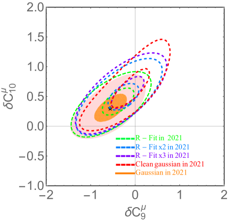
Figure 4: Contour plots at the $1\sigma$ and $3\sigma$ confidence level for the $(\delta C_{9}^{\mu},\delta C_{10}^{\mu})$ scenario in the global fit. For comparison, we show the clean fit (dashed lines in red) in the Gaussian method, and global fits with all observables using the Gaussian (regions in light red and orange) and $R$-fit methods with nominal hadronic uncertainties in $B\to K^{(*)}\ell\ell$ (dashed lines in green), or multiplied by 2 (dashed lines in blue) and 3 (dashed lines in purple).

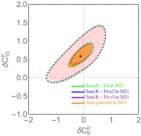
Figure 5: Contour plots at the $1\sigma$ and $3\sigma$ confidence level for the $(\delta C_{9}^{\mu},\delta C_{10}^{\mu})$ scenario in the clean fit. For comparison, we show the clean fits using the Gaussian (regions in light red and orange) and $R$-fit methods with nominal hadronic uncertainties in $B\to K^{(*)}\ell\ell$ (dashed lines in green, corresponding to $\chi^{2}_{\rm SM,min}=30.54$ and $p$-value${}_{\rm SM}=7.6\times 10^{-5}$), or multiplied by 2 (dashed lines in blue, corresponding to $\chi^{2}_{\rm SM,min}=29.99$ and $p$-value${}_{\rm SM}=9.5\times 10^{-5}$) and 3 (dashed lines in purple, corresponding to $\chi^{2}_{\rm SM,min}=29.54$ and $p$-value${}_{\rm SM}=1.15\times 10^{-4}$).

Table 4: Same as Table 3 but for the $R$-fit method with nominal hadronic uncertainties as given in Ref. Geng et al. (2017). One obtains $\chi^{2}_{\rm min,SM}=121.19$, corresponding to a $p$-value of 0.03.

Coefficient	Best fit	$\chi^{2}_{\rm min}$	$p$-value	${\rm Pull}_{\rm SM}$	1$\sigma$ range	3$\sigma$ range
$\delta C_{9}^{\mu}$	$-0.86$	102.3 [93 d.o.f.]	0.24	4.35	$[-1.10,-0.69]$	$[-1.61,-0.24]$
$\delta C_{10}^{\mu}$	0.56	99.24 [93 d.o.f.]	0.31	4.69	[0.45, 0.67]	[0.24, 0.96]
$\delta C_{L}^{\mu}$	$-0.40$	96.32 [93 d.o.f.]	0.39	4.99	$[-0.48,-0.32]$	$[-0.64,-0.16]$
$(\delta C_{9}^{\mu},\delta C_{10}^{\mu})$	$(-0.51,0.36)$	96.17 [92 d.o.f.]	0.36	4.63	$\delta C_{9}^{\mu}\in$ $[-0.63,-0.19]$	$\delta C_{10}^{\mu}\in$[0.24, 0.54]

Table 5: Same as Table 3 but for the $R$-fit method with hadronic uncertainties of $B\to K^{(*)}\ell\ell$ multiplied by 2. One obtains $\chi^{2}_{\rm min,SM}=117.18$, corresponding to a $p$-value of 0.05.

Coefficient	Best fit	$\chi^{2}_{\rm min}$	$p$-value	${\rm Pull}_{\rm SM}$	1$\sigma$ range	3$\sigma$ range
$\delta C_{9}^{\mu}$	$-0.88$	99.95 [93 d.o.f.]	0.29	4.15	$[-1.11,-0.68]$	$[-1.63,-0.22]$
$\delta C_{10}^{\mu}$	0.58	93.18 [93 d.o.f.]	0.48	4.90	[0.48, 0.66]	[0.23, 0.99]
$\delta C_{L}^{\mu}$	$-0.40$	92.90 [93 d.o.f.]	0.48	4.93	$[-0.48,-0.32]$	$[-0.64,-0.16]$
$(\delta C_{9}^{\mu},\delta C_{10}^{\mu})$	$(-0.19,0.60)$	92.19 [92 d.o.f.]	0.47	4.63	$\delta C_{9}^{\mu}\in$ $[-0.53,0.00]$	$\delta C_{10}^{\mu}\in$[0.32, 0.71]

Table 6: Same as Table 3 but for the $R$-fit method with hadronic uncertainties of $B\to K^{(*)}\ell\ell$ multiplied by 3. One obtains $\chi^{2}_{\rm min,SM}=115.03$, corresponding to a $p$-value of 0.07.

Coeff.	best fit	$\chi^{2}_{\rm min}$	$p$-value	${\rm Pull}_{\rm SM}$	1$\sigma$ range	3$\sigma$ range
$\delta C_{9}^{\mu}$	$-0.86$	97.52 [93 d.o.f.]	0.35	4.18	$[-1.10,-0.68]$	$[-1.64,-0.23]$
$\delta C_{10}^{\mu}$	0.70	89.40 [93 d.o.f.]	0.59	5.06	[0.61, 0.81]	[0.27, 1.02]
$\delta C_{L}^{\mu}$	$-0.41$	90.27 [93 d.o.f.]	0.56	4.98	$[-0.49,-0.33]$	$[-0.65,-0.17]$
$(\delta C_{9}^{\mu},\delta C_{10}^{\mu})$	$(0.02,0.70)$	89.37 [92 d.o.f.]	0.56	4.69	$\delta C_{9}^{\mu}\in$ $[-0.28,0.13]$	$\delta C_{10}^{\mu}\in$[0.39, 0.82]

VII Summary and outlook

In conclusion, we have presented a statistical analysis of recent data on LUV ratios and $B_{s}\to\mu\mu$ using the low-energy $b\to s\ell\ell$ effective Lagrangian. We find that the data on these clean observables disagree with the SM at a level of $4.0\sigma$. Scenarios with pure left-handed or axial currents provide a good description of the data, and each of them excludes the SM point at $\sim 5\sigma$ confidence level. Therefore, our results reinforce the NP interpretation of the anomalies in the $b\to s\ell\ell$ transitions, which could correspond to the contribution of the tree-level exchange of a leptoquark or $Z^{\prime}$ with a mass $\Lambda\sim 30$ TeV and $\sim\mathcal{O}(1)$ couplings to the SM. Further data on LUV observables from LHCb and Belle II should be able to clarify soon this tantalizing possibility.

VIII Acknowledgments

We would like to thank A. Cerri, M. Bona and R. Zwicky for helpful conversations and P. Hernández for useful comments. This work is partly supported by the National Natural Science Foundation of China under Grants No. 11735003, No. 11975041, and No.11961141004, the Academic Excellence Foundation of BUAA for Ph.D. students, and the fundamental Research Funds for the Central Universities. The work of B.G. is supported in part by the U.S. Department of Energy Grant No. DE-SC0009919. S.J. is supported in part by the U.K. Science and Technology Facilities Council under Consolidated Grants No. ST/P000819/1 and No. ST/T00102X/1. J.M.C. acknowledges support from the Spanish MINECO through the “Ramón y Cajal” Program No. RYC-2016-20672 and Grant No. PGC2018-102016-A-I00.

$Note~{}added.$-Recently, several other papers appeared performing similar global fits and finding very similar conclusions Angelescu et al. (2021); Altmannshofer and Stangl (2021); Cornella et al. (2021); Kriewald et al. (2021); Lancierini et al. (2021); Hurth et al. (2021); Algueró et al. (2021).

IX Appendix: Updated clean fits after the latest LHCb measurements of $R_{K^{0}_{s}}$ and $R_{K^{*+}}$

In this section, we show that the latest measurements of the branching fraction ratios $R_{K^{0}_{s}}$ and $R_{K^{*+}}$, in combination with the already known ratios $R_{K^{+}}$, $R_{K^{*0}}$, and the branching fraction $B_{s}\to\mu\mu$, point at a discrepancy with the Standard Model at $4.2\sigma$. One-parameter scenarios, $C_{10}^{\mu}$ and $C_{L}^{\mu}$, fit the data well and result in a pull from the SM crossing the 5.0$\sigma$ threshold. The two-parameter fit of $C_{9}$ and $C_{10}$ yields also a pull of 5.02$\sigma$. On the other hand, the one-parameter scenario of $C_{9}$ alone still has a pull of 4.5$\sigma$, up from the previous 4.1$\sigma$ (see Table II).

Very recently, the LHCb Collaboration reported measurements of two new lepton-universality ratios $R_{K_{S}^{0}}=\Gamma(B^{0}\to K_{S}^{0}\mu^{+}\mu^{-})/\Gamma(B^{0}\to K_{S}^{0}e^{+}e^{-})$ and $R_{K^{*+}}=\Gamma(B^{+}\to K^{*+}\mu^{+}\mu^{-})/\Gamma(B^{+}\to K^{*+}e^{+}e^{-})$ in the $q^{2}$ ranges $[1.1,6.0]~{}{\rm GeV}^{2}$ and $[0.045,6.0]~{}{\rm GeV}^{2}$, respectively, using proton-proton collision data corresponding to an integrated luminosity of 9 fb^-1 Aaij et al. (2021b). They represent the first observation of the $B^{0}\to K_{s}^{0}e^{+}e^{-}$ and $B^{+}\to K^{*+}e^{+}e^{-}$ decays. The two ratios are

$$R_{K_{S}^{0}}=0.66_{~{}-0.14~{}-0.04}^{~{}+0.20~{}+0.02},$$

$$R_{K^{*+}}=0.70_{~{}-0.13~{}-0.04}^{~{}+0.18~{}+0.03},$$ (26)

where the first error is statistical and the second is systematic. These results show again tension with respect to the SM predictions (see Table I) with a significance of $1.5\sigma$ and $1.4\sigma$, respectively. In the following analysis, we conservatively employ a symmetric error equal to the larger error.

It should be noted that these ratios are the isospin partners of $R_{K^{+}}$ and $R_{K^{*0}}$, and therefore should receive the same NP contributions, if they exist. As a result, it is of utmost importance to update the clean fit performed in the main text and to check whether these new measurements increase or decrease the significance of the tension with the SM.

Note that compared to the clean fit performed in the main text, the total number of fitted data becomes 9 after adding the two new LHCb measurements. Setting the Wilson coefficients to their SM values, we obtain a $\chi^{2}_{\rm min,SM}=36.50$, corresponding to a $p$-value of $3.23\times 10^{-5}$ or a $4.2\sigma$ deviation (for 9 d.o.f.). As a result, with the new data, the LU ratios are in discrepancy with the SM predictions at a level of $4.2\sigma$, up from the $4.0\sigma$ in March 2021.

In Table 7 and Fig. 6, we show the results of four fits which are obtained by allowing for lepton-specific contributions $\delta C_{9}^{\mu}$, $\delta C_{10}^{\mu}$, $\delta C_{L}^{\mu}$ and a two-dimensional scenario $(\delta C_{9}^{\mu},\delta C_{10}^{\mu})$. We find that the significance of all the NP scenarios except for $\delta C_{9}^{\mu}$ are more than $5\sigma$. Such a result, obtained by considering only clean observables, seems to point unambiguously to the presence of new physics. We conclude that although the newly observed ratios are the isospin partners of the existing ones, they indeed have increased the significance of the tension with the SM by about $0.5\sigma$ compared with the fits without them in March 2021.

Table 7: Same as Table 2 but fitted also to the latest LHCb data $R_{K_{S}^{0}}$ and $R_{K^{*+}}$.

Coefficient	Best fit	$\chi^{2}_{\rm min}$	$p$-value	${\rm Pull}_{\rm SM}$	1$\sigma$ range	3$\sigma$ range	$\rho$
$\delta C_{9}^{\mu}$	$-0.89$	16.27 [8 d.o.f.]	0.04	4.50	$[-1.12,-0.67]$	$[-1.67,~{}-0.27]$	$\cdots$
$\delta C_{10}^{\mu}$	0.69	7.84   [8 d.o.f.]	0.45	5.35	$[0.57,0.84]$	$[0.29,1.16]$	$\cdots$
$\delta C_{L}^{\mu}$	$-0.42$	8.45 [8 d.o.f.]	0.39	5.30	$[-0.51,-0.34]$	$[-0.69,-0.18]$	$\cdots$
$(\delta C_{9}^{\mu},\delta C_{10}^{\rm\mu})$	$(-0.15,0.60)$	$7.56$ [7 d.o.f.]	$0.37$	$5.02$	$\delta C_{9}^{\mu}\in$ $[-0.45,~{}0.13]$	$\delta C_{10}^{\mu}\in$ $[0.10,~{}1.01]$	$0.765$

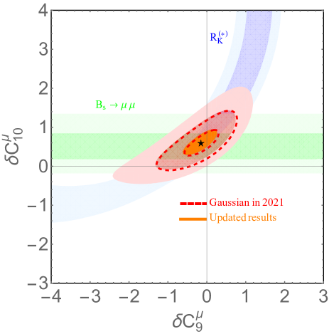
Figure 6: Same as Fig. 2 but for the new clean fit to 9 data including the latest LHCb measurements Aaij et al. (2021b) vs. the clean fit to 7 data shown in Fig. 2 (Gaussian in 2021).

References

- Buras (2020) A. Buras, Gauge Theory of Weak Decays (Cambridge University Press, 2020).
- Geng et al. (2017) L.-S. Geng, B. Grinstein, S. Jäger, J. Martin Camalich, X.-L. Ren, and R.-X. Shi, Phys. Rev. D 96, 093006 (2017), arXiv:1704.05446 [hep-ph] .
- Bifani et al. (2019) S. Bifani, S. Descotes-Genon, A. Romero Vidal, and M.-H. Schune, J. Phys. G 46, 023001 (2019), arXiv:1809.06229 [hep-ex] .
- Hiller and Kruger (2004) G. Hiller and F. Kruger, Phys. Rev. D69, 074020 (2004), arXiv:hep-ph/0310219 [hep-ph] .
- Beneke et al. (2018) M. Beneke, C. Bobeth, and R. Szafron, Phys. Rev. Lett. 120, 011801 (2018), arXiv:1708.09152 [hep-ph] .
- Aaij et al. (2021a) R. Aaij et al. (LHCb), (2021a), arXiv:2103.11769 [hep-ex] .
- Bordone et al. (2016) M. Bordone, G. Isidori, and A. Pattori, Eur. Phys. J. C 76, 440 (2016), arXiv:1605.07633 [hep-ph] .
- Isidori et al. (2020) G. Isidori, S. Nabeebaccus, and R. Zwicky, JHEP 12, 104 (2020), arXiv:2009.00929 [hep-ph] .
- Aaij et al. (2014) R. Aaij et al. (LHCb), Phys. Rev. Lett. 113, 151601 (2014), arXiv:1406.6482 [hep-ex] .
- Santimaria (2021) M. Santimaria, in LHCb Seminar at CERN (March 23th 2021).
- Aaboud et al. (2019) M. Aaboud et al. (ATLAS), JHEP 04, 098 (2019), arXiv:1812.03017 [hep-ex] .
- Sirunyan et al. (2020) A. M. Sirunyan et al. (CMS), JHEP 04, 188 (2020), arXiv:1910.12127 [hep-ex] .
- Beneke et al. (2019) M. Beneke, C. Bobeth, and R. Szafron, JHEP 10, 232 (2019), arXiv:1908.07011 [hep-ph] .
- Abdesselam et al. (2019a) A. Abdesselam et al. (Belle), (2019a), arXiv:1908.01848 [hep-ex] .
- Aaij et al. (2017a) R. Aaij et al. (LHCb), JHEP 08, 055 (2017a), arXiv:1705.05802 [hep-ex] .
- Abdesselam et al. (2019b) A. Abdesselam et al. (Belle), (2019b), arXiv:1904.02440 [hep-ex] .
- Aaij et al. (2020a) R. Aaij et al. (LHCb), Phys. Rev. Lett. 125, 011802 (2020a), arXiv:2003.04831 [hep-ex] .
- Aaij et al. (2020b) R. Aaij et al. (LHCb), (2020b), arXiv:2012.13241 [hep-ex] .
- D’Amico et al. (2017) G. D’Amico, M. Nardecchia, P. Panci, F. Sannino, A. Strumia, R. Torre, and A. Urbano, JHEP 09, 010 (2017), arXiv:1704.05438 [hep-ph] .
- Ciuchini et al. (2020) M. Ciuchini, M. Fedele, E. Franco, A. Paul, L. Silvestrini, and M. Valli, (2020), arXiv:2011.01212 [hep-ph] .
- Munir Bhutta et al. (2020) F. Munir Bhutta, Z.-R. Huang, C.-D. Lü, M. A. Paracha, and W. Wang, (2020), arXiv:2009.03588 [hep-ph] .
- Bečirević et al. (2020) D. Bečirević, S. Fajfer, N. Košnik, and A. Smolkovič, Eur. Phys. J. C 80, 940 (2020), arXiv:2008.09064 [hep-ph] .
- Alasfar et al. (2020) L. Alasfar, A. Azatov, J. de Blas, A. Paul, and M. Valli, JHEP 12, 016 (2020), arXiv:2007.04400 [hep-ph] .
- Hurth et al. (2020) T. Hurth, F. Mahmoudi, and S. Neshatpour, Phys. Rev. D 102, 055001 (2020), arXiv:2006.04213 [hep-ph] .
- Bhom et al. (2020) J. Bhom, M. Chrzaszcz, F. Mahmoudi, M. Prim, P. Scott, and M. White, (2020), arXiv:2006.03489 [hep-ph] .
- Descotes-Genon et al. (2020) S. Descotes-Genon, S. Fajfer, J. F. Kamenik, and M. Novoa-Brunet, Phys. Lett. B 809, 135769 (2020), arXiv:2005.03734 [hep-ph] .
- Biswas et al. (2020) A. Biswas, S. Nandi, I. Ray, and S. K. Patra, (2020), arXiv:2004.14687 [hep-ph] .
- Bordone et al. (2020) M. Bordone, O. Catà, and T. Feldmann, JHEP 01, 067 (2020), arXiv:1910.02641 [hep-ph] .
- Coy et al. (2020) R. Coy, M. Frigerio, F. Mescia, and O. Sumensari, Eur. Phys. J. C 80, 52 (2020), arXiv:1909.08567 [hep-ph] .
- Bhattacharya et al. (2020) S. Bhattacharya, A. Biswas, S. Nandi, and S. K. Patra, Phys. Rev. D 101, 055025 (2020), arXiv:1908.04835 [hep-ph] .
- Arbey et al. (2019) A. Arbey, T. Hurth, F. Mahmoudi, D. M. Santos, and S. Neshatpour, Phys. Rev. D 100, 015045 (2019), arXiv:1904.08399 [hep-ph] .
- Kowalska et al. (2019) K. Kowalska, D. Kumar, and E. M. Sessolo, Eur. Phys. J. C 79, 840 (2019), arXiv:1903.10932 [hep-ph] .
- Algueró et al. (2019a) M. Algueró, B. Capdevila, A. Crivellin, S. Descotes-Genon, P. Masjuan, J. Matias, M. Novoa Brunet, and J. Virto, Eur. Phys. J. C 79, 714 (2019a), [Addendum: Eur.Phys.J.C 80, 511 (2020)], arXiv:1903.09578 [hep-ph] .
- Aebischer et al. (2020) J. Aebischer, W. Altmannshofer, D. Guadagnoli, M. Reboud, P. Stangl, and D. M. Straub, Eur. Phys. J. C 80, 252 (2020), arXiv:1903.10434 [hep-ph] .
- Ciuchini et al. (2019) M. Ciuchini, A. M. Coutinho, M. Fedele, E. Franco, A. Paul, L. Silvestrini, and M. Valli, Eur. Phys. J. C 79, 719 (2019), arXiv:1903.09632 [hep-ph] .
- Alok et al. (2019) A. K. Alok, A. Dighe, S. Gangal, and D. Kumar, JHEP 06, 089 (2019), arXiv:1903.09617 [hep-ph] .
- Algueró et al. (2019b) M. Algueró, B. Capdevila, S. Descotes-Genon, P. Masjuan, and J. Matias, JHEP 07, 096 (2019b), arXiv:1902.04900 [hep-ph] .
- Kumar and London (2019) J. Kumar and D. London, Phys. Rev. D 99, 073008 (2019), arXiv:1901.04516 [hep-ph] .
- Datta et al. (2019) A. Datta, J. Kumar, and D. London, Phys. Lett. B 797, 134858 (2019), arXiv:1903.10086 [hep-ph] .
- Beneke et al. (2001) M. Beneke, T. Feldmann, and D. Seidel, Nucl. Phys. B 612, 25 (2001), arXiv:hep-ph/0106067 .
- Grinstein and Pirjol (2004) B. Grinstein and D. Pirjol, Phys. Rev. D70, 114005 (2004), arXiv:hep-ph/0404250 [hep-ph] .
- Egede et al. (2008) U. Egede, T. Hurth, J. Matias, M. Ramon, and W. Reece, JHEP 11, 032 (2008), arXiv:0807.2589 [hep-ph] .
- Khodjamirian et al. (2010) A. Khodjamirian, T. Mannel, A. Pivovarov, and Y.-M. Wang, JHEP 09, 089 (2010), arXiv:1006.4945 [hep-ph] .
- Beylich et al. (2011) M. Beylich, G. Buchalla, and T. Feldmann, Eur. Phys. J. C71, 1635 (2011), arXiv:1101.5118 [hep-ph] .
- Khodjamirian et al. (2013) A. Khodjamirian, T. Mannel, and Y. M. Wang, JHEP 02, 010 (2013), arXiv:1211.0234 [hep-ph] .
- Descotes-Genon et al. (2013) S. Descotes-Genon, J. Matias, M. Ramon, and J. Virto, JHEP 01, 048 (2013), arXiv:1207.2753 [hep-ph] .
- Jäger and Martin Camalich (2013) S. Jäger and J. Martin Camalich, JHEP 05, 043 (2013), arXiv:1212.2263 [hep-ph] .
- Horgan et al. (2014) R. R. Horgan, Z. Liu, S. Meinel, and M. Wingate, Phys. Rev. Lett. 112, 212003 (2014), arXiv:1310.3887 [hep-ph] .
- Lyon and Zwicky (2014) J. Lyon and R. Zwicky, (2014), arXiv:1406.0566 [hep-ph] .
- Descotes-Genon et al. (2014) S. Descotes-Genon, L. Hofer, J. Matias, and J. Virto, JHEP 12, 125 (2014), arXiv:1407.8526 [hep-ph] .
- Jäger and Martin Camalich (2016) S. Jäger and J. Martin Camalich, Phys. Rev. D 93, 014028 (2016), arXiv:1412.3183 [hep-ph] .
- Bharucha et al. (2016) A. Bharucha, D. M. Straub, and R. Zwicky, JHEP 08, 098 (2016), arXiv:1503.05534 [hep-ph] .
- Ciuchini et al. (2016) M. Ciuchini, M. Fedele, E. Franco, S. Mishima, A. Paul, L. Silvestrini, and M. Valli, JHEP 06, 116 (2016), arXiv:1512.07157 [hep-ph] .
- Hiller and Nisandzic (2017) G. Hiller and I. Nisandzic, Phys. Rev. D 96, 035003 (2017), arXiv:1704.05444 [hep-ph] .
- Chobanova et al. (2017) V. G. Chobanova, T. Hurth, F. Mahmoudi, D. Martinez Santos, and S. Neshatpour, (2017), arXiv:1702.02234 [hep-ph] .
- Bobeth et al. (2018) C. Bobeth, M. Chrzaszcz, D. van Dyk, and J. Virto, Eur. Phys. J. C 78, 451 (2018), arXiv:1707.07305 [hep-ph] .
- Aaij et al. (2017b) R. Aaij et al. (LHCb), Eur. Phys. J. C 77, 161 (2017b), arXiv:1612.06764 [hep-ex] .
- Gubernari et al. (2019) N. Gubernari, A. Kokulu, and D. van Dyk, JHEP 01, 150 (2019), arXiv:1811.00983 [hep-ph] .
- Cerri et al. (2019) A. Cerri et al., CERN Yellow Rep. Monogr. 7, 867 (2019), arXiv:1812.07638 [hep-ph] .
- LHC (2020) “Combination of the ATLAS, CMS and LHCb results on the decays,” (2020).
- Buchalla et al. (1996) G. Buchalla, A. J. Buras, and M. E. Lautenbacher, Rev. Mod. Phys. 68, 1125 (1996), arXiv:hep-ph/9512380 .
- Alonso et al. (2014) R. Alonso, B. Grinstein, and J. Martin Camalich, Phys. Rev. Lett. 113, 241802 (2014), arXiv:1407.7044 [hep-ph] .
- Ball and Zwicky (2005) P. Ball and R. Zwicky, Phys. Rev. D 71, 014029 (2005), arXiv:hep-ph/0412079 .
- Aaij et al. (2019) R. Aaij et al. (LHCb), Phys. Rev. Lett. 122, 191801 (2019), arXiv:1903.09252 [hep-ex] .
- Aaboud et al. (2018) M. Aaboud et al. (ATLAS), JHEP 10, 047 (2018), arXiv:1805.04000 [hep-ex] .
- Angelescu et al. (2021) A. Angelescu, D. Bečirević, D. A. Faroughy, F. Jaffredo, and O. Sumensari, (2021), arXiv:2103.12504 [hep-ph] .
- Altmannshofer and Stangl (2021) W. Altmannshofer and P. Stangl, (2021), arXiv:2103.13370 [hep-ph] .
- Cornella et al. (2021) C. Cornella, D. A. Faroughy, J. Fuentes-Martín, G. Isidori, and M. Neubert, (2021), arXiv:2103.16558 [hep-ph] .
- Kriewald et al. (2021) J. Kriewald, C. Hati, J. Orloff, and A. M. Teixeira, in 55th Rencontres de Moriond on Electroweak Interactions and Unified Theories (2021) arXiv:2104.00015 [hep-ph] .
- Lancierini et al. (2021) D. Lancierini, G. Isidori, P. Owen, and N. Serra, (2021), arXiv:2104.05631 [hep-ph] .
- Hurth et al. (2021) T. Hurth, F. Mahmoudi, D. M. Santos, and S. Neshatpour, (2021), arXiv:2104.10058 [hep-ph] .
- Algueró et al. (2021) M. Algueró, B. Capdevila, S. Descotes-Genon, J. Matias, and M. Novoa-Brunet, in 55th Rencontres de Moriond on QCD and High Energy Interactions (2021) arXiv:2104.08921 [hep-ph] .
- Aaij et al. (2021b) R. Aaij et al. (LHCb), (2021b), arXiv:2110.09501 [hep-ex] .