sok: Decentralized Exchanges (DEX) with Automated Market Maker (amm) Protocols

Abstract.

As an integral part of the defi ecosystem, dex with amm protocols have gained massive traction with the recently revived interest in blockchain and dlt in general. Instead of matching the buy and sell sides, amm employ a peer-to-pool method and determine asset price algorithmically through a so-called conservation function. To facilitate the improvement and development of amm-based dex, we create the first systematization of knowledge in this area. We first establish a general amm framework describing the economics and formalizing the system’s state-space representation. We then employ our framework to systematically compare the top amm protocols’ mechanics, illustrating their conservation functions, as well as slippage and divergence loss functions. We further discuss security and privacy concerns, how they are enabled by amm-based dex’ inherent properties, and explore mitigating solutions. Finally, we conduct a comprehensive literature review on related work covering both defi and conventional market microstructure.

1. Introduction

With the revived interest in blockchain and cryptocurrency among both the general populace and institutional actors, the past year has witnessed a surge in crypto trading activity and accelerated development in the defi space. Among all the prominent defi applications, dex with amm protocols are in the ascendancy, with an aggregate value locked exceeding $100 billion at the time of writing (202, 2021a).

An amm-based dex bears attractive features such as decentralization, automation and continuous liquidity. With traditional order-book-based exchanges, the market price of an asset is determined by the last matched buy and sell orders, ultimately driven by the supply and demand of the asset. In contrast, on an amm-based dex, a liquidity pool acts as a single counterparty for each transaction, with a so-called conservation function that prices assets algorithmically by only allowing the price to move along predefined trajectories. amm implement a peer-to-pool method, where lp contribute assets to liquidity pools while individual users exchange assets with a pool or pools containing the input and the output assets. Users obtain immediate liquidity without having to find an exchange counterparty, whereas lp profit from asset supply with exchange fees from users. Furthermore, by using a conservation function for price setting, amm render moot the necessity of maintaining the state of an order book, which would be costly on a distributed ledger.

amm benefit both lp and exchange users with accessible liquidity provision and exchange, especially for illiquid assets. Despite the apparent advantages, amm are often characterized by high slippage and divergence loss, two implicit economic risks imposed on the funds of exchange users and lp respectively. Moreover, amm-based dex are associated with myriads of security and privacy issues. Throughout the last three years, new protocols have been introduced to the market one after another with incremental improvements, attempting to tackle different issues which had been identified as weak spots in a previous version. On top of that, new use cases are being addressed, and new applications of amm iterations are proposed to the market. While innovative in certain aspects, the various amm protocols generally consist of the same set of composed mechanisms to allow for multiple functionalities of the system. As such, these systems are structurally similar, and their main differences lie in parameter choices and/or mechanism adaptations.

As one of the earliest defi application categories, amm-based dex also constitute the most fundamental and crucial building blocks of the defi ecosystem. Their importance prompts the emergence of studies covering various aspects of amm-based dex: economics (Bartoletti et al., 2021b), security (Zhou et al., 2021a; Yüksel et al., 2021; Zhou et al., 2021c), privacy (Baum et al., 2021b; Bowe et al., 2020), etc. While there has arisen a large number of surveys on general defi (Sam M. Werner et al., 2022; Schär, 2021) as well as various defi applications (Cousaert et al., 2022b; Bartoletti et al., 2021a), there is a dearth of literature that systematically studies and critically examines dex with amm protocols in a comprehensive manner. To the best of our knowledge, this paper fills this gap as the first sok on amm-based dex with examples of deployed protocols. We contribute to the body of literature mainly by:

1. generalizing mechanisms and economics of amm-based dex with a formalized state space modeling framework and a summary of key common properties;

2. illustrating instantiations of our framework by comparing major amm-based dex with mathematical derivation and parameterized visualization on their conservation function, slippage and divergence loss functions;

3. positioning amm-based dex within the broader taxonomy of defi, and examining their relationships and interactions with other defi protocols;

4. establishing a taxonomy of security and privacy issues concerning amm-based dex, and exploring mitigation solutions;

5. conducting a state-of-the-art literature review summarizing current research priorities as well as existing output in amm-based dex and related fields, and identifying potential directions for future research.

The rest of the paper is structured as follows: in §2 we lay out fundamental concepts and components of amm; in §3 we formalize amm mechanisms with a state-space representation; in §4 we compare main protocols in terms of conservation function, exchange rates, slippage and impermanent loss; in §5 we address issues related to security and privacy of amm-based dex; in §6 we indicate several avenues of future amm research; in §7 we present related work; in §8 we conclude.

2. AMM Preliminaries

This section presents amm-based dex’ main components, including different actors and assets, as well as their generalized mechanism and economics.

2.1. Actors

2.1.1. lp

A liquidity pool can be deployed through a smart contract with some initial supply of crypto assets by the first lp. Other lp can subsequently increase the pool’s reserve by adding more of the type of assets that are contained in the pool. In turn, they receive pool shares proportionate to their liquidity contribution as a fraction of the entire pool (Evans, 2020). lp earn transaction fees paid by exchange users. While sometimes subject to a withdrawal penalty, lp can freely remove funds from the pool (Martinelli and Mushegian, 2019) by surrendering a corresponding amount of pool shares (Evans, 2020).

2.1.2. Exchange user (Trader)

A trader submits an exchange order to a liquidity pool by specifying the input and output asset and either an input asset or output asset quantity; the smart contract automatically calculates the exchange rate based on the conservation function as well as the transaction fee and executes the exchange order accordingly.

Arbitrageurs compare asset prices across different markets to execute trades whenever closing price gaps can extract profits (Makarov and Schoar, 2020). amm such as DODO (see §4.1.5) leverage users’ arbitrage behavior through their protocol design.

2.1.3. Protocol foundation

A protocol foundation consists of protocol founders, designers, and developers responsible for architecting and improving the protocol. The development activities are often funded directly or indirectly through accrued earnings such that the foundation members are financially incentivized to build a user-friendly protocol that can attract high trading volume.

2.2. Assets

Several distinct types of assets are used in amm protocols for operations and governance; one asset may assume multiple roles.

2.2.1. Risk assets

Characterized by illiquidity, risk assets are the primary type of assets amm-based dex are designed for. Like centralized exchanges, an amm-based dex can facilitate an ieo to launch a new token through liquidity pool creation, a capital raising activity termed “ido” that is particularly suitable for illiquid assets. To be eligible for an ido, a risk asset sometimes needs to be whitelisted, and must be compatible with the protocol’s technical requirements (e.g. ERC20 (202, 2021b) for most amm on Ethereum).

2.2.2. Base assets

Some protocols require a trading pair always to consist of a risk asset and a designated base asset. In the case of Bancor, every risk asset is paired with BNT, the protocol’s native token (Bancor, 2020b). Uniswap V1 requires every pool to be initiated with a risk asset paired with ETH. Many protocols, such as Balancer and Curve, can connect two or more risk assets directly in liquidity pools without a designated base asset.

2.2.3. Pool shares

Also known as “liquidity shares” and “lp shares”, pool shares represent ownership in the portfolio of assets within a pool, and are distributed to lp. Shares accrue trading fees proportionally and can be redeemed at any time to withdraw funds from the pool.

2.2.4. Protocol tokens

Protocol tokens are used to represent voting rights on protocol governance matters and are thus also termed “governance tokens” (see §2.4.1). Protocol tokens are typically valuable assets (Xu et al., 2022) that are tradeable outside of the amm and can incentivize participation when e.g. rewarded to lp proportionate to their liquidity supply. amm compete with each other to attract funds and trading volume. To bootstrap an amm in the early phase with incentivized early pool establishment and trading, a feature called liquidity mining can be installed where the native protocol’s tokens are minted and issued to lp and/or exchange users.

2.3. Fundamental amm dynamics

2.3.1. Invariant properties

The functionality of an amm depends upon a conservation function which encodes a desired invariant property of the system. As an intuitive example, Uniswap’s constant product function determines trading dynamics between assets in the pool as it always conserves the product of value-weighted quantities of both assets in the protocol—each trade has to be made in a way such that the value removed in one asset equals the value added in the other asset. This weight-preserving characteristic is one desired invariant property supported by the design of Uniswap.

2.3.2. Mechanisms

An amm typically involves two types of interaction mechanism: asset swapping of assets and liquidity provision/withdrawal. Interaction mechanisms have to be specified in a way such that desired invariant properties are upheld; therefore the class of admissible mechanisms is restricted to the ones which respect the defined conservation function, if one is specified, or conserve the defined properties otherwise.

2.4. Fundamental amm economics

2.4.1. Rewards

amm protocols often run several reward schemes, including liquidity reward, staking reward, governance rights and security reward distributed to different actors to encourage participation and contribution.

Liquidity reward

lp are rewarded for supplying assets to a liquidity pool, as they have to bear the opportunity costs associated with funds being locked in the pool. lp receive their share of trading fees paid by exchange users.

Staking reward

On top of the liquidity reward in the form of transaction income, lp are offered the possibility to stake pool shares or other tokens as part of an initial incentive program from a certain token protocol. The ultimate goal of the individual token protocols (see e.g. GIV (CryptoLocally, 2020) and TRIPS (De Giglio, 2021)) is to further encourage token holding, while simultaneously facilitating token liquidity on exchanges and product usage. These staking rewards are given by protocols other than the amm.

Governance right

An amm may encourage liquidity provision and/or swapping by rewarding participants governance rights in the form of protocol tokens (see §2.2.4). Currently, governance issues such as protocol treasury management (demosthenes.eth, 2021) are proposed and discussed mostly on off-chain governance portals such as snapshot (snapshot.org), Tally (tally.xyz) and Boardroom (boardroom.io), where protocol tokens are used as ballots (see §2.2.4) to vote on proposals.

Security reward

Just as every protocol built on top of an open, distributed network, amm-based dex on Ethereum suffer from security vulnerabilities. Besides code auditing, a common practice that a protocol foundation adopts is to have the code vetted by a broader developer community and reward those who discover and/or fix bugs of the protocol with monetary prizes, commonly in fiat currencies, through a bounty program (Breidenbach et al., 2018).

2.4.2. Explicit costs

Interacting with amm protocols incurs various costs, including charges for some form of “value” created or “service” performed and fees for interacting with the blockchain network. amm participants need to anticipate three types of fees: liquidity withdrawal penalty, swap fee and gas fee.

Liquidity withdrawal penalty

As introduced in §3.2 and further discussed in §4 of this paper, withdrawal of liquidity changes the shape of the conservation function and negatively affects the usability of the pool by elevating slippage. Therefore, amm such as DODO (DODO Team, 2020) levy a liquidity withdrawal penalty.

Swap fee

Users interacting with the liquidity pool for token exchanges have to reimburse lp for the supply of assets and for the divergence loss (see §2.4.3). This compensation comes in the form of swap fees that are charged in every exchange trade and then distributed to liquidity pool shareholders. A small percentage of the swap fees may also go to the foundation of the amm to further develop the protocol (Xu and Xu, 2022).

Gas fee

Every interaction with the protocol is executed in the form of an on-chain transaction, and is thus subject to a gas fee applicable to all transactions on the underlying blockchain. In a decentralized network, validating nodes need to be compensated for their efforts, and transaction initiators must cover these operating costs. Interacting with more complex protocols will result in a higher gas fee due to the higher computational power needed for transaction verification.

2.4.3. Implicit costs

Two essential implicit costs native to amm-based dex are slippage for exchange users and divergence loss for lp.

Slippage

Slippage is defined as the difference between the spot price and the realized price of a trade. Instead of matching buy and sell orders, amm determine exchange rates on a continuous curve, and every trade will encounter slippage conditioned upon the trade size relative to the pool size and the exact design of the conservation function. The spot price approaches the realized price for infinitesimally small trades, but they deviate more for bigger trade sizes. This effect is amplified for smaller liquidity pools as every trade will significantly impact the relative quantities of assets in the pool, leading to higher slippage. Due to continuous slippage, trades on amm must be set with some slippage tolerance to be executed, a feature that can be exploited to perform e.g. sandwich attacks (see §5.1.3).

Divergence loss

For lp, assets supplied to a protocol are still exposed to volatility risk, which comes into play in addition to the loss of time value of locked funds. A swap alters the asset composition of a pool, which automatically updates the asset prices implied by the conservation function of the pool (Eq. 3). This consequently changes the value of the entire pool. Compared to holding the assets outside of an amm pool, contributing the same amount of assets to the pool in return for pool shares can result in less value with price movement, an effect termed “divergence loss” or “impermanent loss” (see §4). This loss can be deemed “impermanent” because as asset price moves back and forth, the depreciation of the pool value continuously disappears and reappears and is only realized when assets are actually taken out of the pool. Well-devised amm charge appropriate swap fees to ensure that lp are sufficiently compensated for the divergence loss (see §4.2.2). Despite the fact that “impermanent loss” is a more widely used term on the Internet, we adhere to the more accurate term “divergence loss” in a scientific context. In fact, for the majority of amm protocols, this “loss” only disappears when the current proportions of the pool assets equal exactly those at liquidity provision, which is rarely the case.

Since assets are bonded together in a pool, changes in prices of one asset affect all others in this pool. For an amm protocol that supports single-asset supply, this forces lp to be exposed to risk assets they have not been holding in the first place (see §3.3.1).

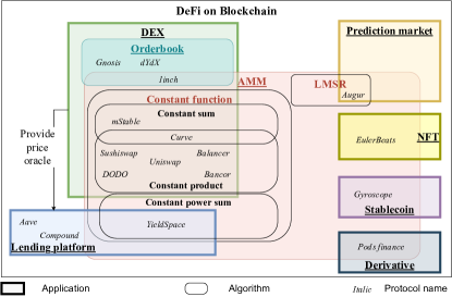
Figure 1. amm-based dex within the broader taxonomy of defi on blockchain. amm as an algorithm and dex as an application are not mutually inclusive.

2.5. amm-based dex within defi

For brevity, we use “amm” or “dex” to refer to amm-based dex throughout the paper, unless indicated otherwise. Nevertheless, it is to be noted that the term “amm” emphasizes the algorithm of a protocol, whereas “dex” emphasizes the use case, or application, of a protocol. Within the context of blockchain-based defi, there also exist orderbook-based dex such as Gnosis and dYdX that do not rely on amm algorithms. Recently, dex aggregators (§4.3.8) such as 1inch have emerged which incorporate both limited order books and amm pools. On the other hand, amm algorithms are also not exclusively employed by dex. defi applications such as lending platforms, nft, stablecoins and derivatives all have protocols that make use of different amm algorithms.

amm can also assume various forms (see §7.2.2). Prediction markets for example commonly employs lmsr, whereas cfmm is the primary underpinning for dex. In particular, constant sum and constant product are the most representative forms of cfmm, widely adopted by amm-based dex protocols. Fig. 1 illustrates amm-based dex within the broader taxonomy of defi on blockchain.

The ensuing sections, §3 and §4, focus on cfmm mechanisms which have been adopted by major dex, with their exact formulas derived in Appendix A. §4.3 briefly presents other defi applications with amm implementations.

3. Formalization of Mechanisms

Overall, the functionality of an amm can be generalized formally by a set of few mechanisms. These mechanisms define how users can interact with the protocol and what the response of the protocol will be given particular user actions.

3.1. State space representation

The functioning of any blockchain-based system can be modeled using state-space terminology. States and agents constitute the main system components; protocol activities are described as actions (Fig. 2); the evolution of the system over time is modeled with state transition functions. This can be generalized into a state transition function $f$ encoded in the protocol such that $\chi\xrightarrow[f]{a}\chi^{\prime}$, where $a\in A$ represents an action imposed on the system while $\chi$ and $\chi^{\prime}$ represent the current and future states of the system respectively.

The object of interest is the state $\chi$ of the liquidity pool which can be described with

(1) $$\chi=(\{r_{k}\}_{k=1,...,n},\{p_{k}\}_{k=1,...,n},{\mathcal{I}},\Omega)$$

where $r_{k}$ denotes the quantity of token_k in the pool, $p_{k}$ the current spot price of token_k, ${\mathcal{I}}$ the conservation function invariant(s), and $\Omega$ the collection of protocol hyperparameters. This formalization can encompass various amm designs.

The most critical design component of an amm is its conservation function which defines the relationship between different state variables and the invariant(s) ${\mathcal{I}}$. The conservation function is protocol-specific as each protocol seeks to prioritize a distinct feature and target particular functionalities (see §4).

The core of an amm system state is the quantity of each asset held in a liquidity pool. Their sums or products are typical candidates for invariants. Examples of a constant-sum market maker include mStable (Andersson, 2020). Uniswap (Uniswap, 2020) represents constant-product market makers, while Balancer (Martinelli and Mushegian, 2019) generalizes this idea to a geometric mean. The Curve (Egorov, 2019) conservation function is notably a combination of constant-sum and constant-product (see §4).

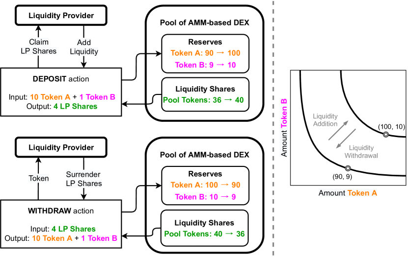
(a) Liquidity provision and withdrawal.

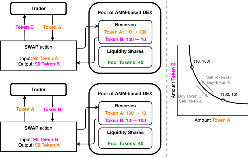
(b) Swap.

Figure 2. Stylized amm mechanisms for lp (§2.1.1) and traders (§2.1.2).

3.2. Generalized formulas

In this section, we generalize amm formulas necessary for demonstrating the interdependence between various amm invariants and state variables, as well as for computing slippage and divergence loss. Mathematical notations and their definitions can be found in Table 1.

Hyperparameter set $\Omega$ is determined at pool creation and shall remain the same afterwards. While the value of hyperparameters might be changed through protocol governance activities, this does not and should not occur on a frequent basis.

Invariant ${\mathcal{I}}$, despite its name, refers to the pool variable that stays constant only with swap actions (see §3.3.2) but changes at liquidity provision and withdrawal. In contrast, trading moves the price of traded assets; specifically, it increases the price of the output asset relative to the input asset, reflecting a value appreciation of the output asset driven by demand (see §3.3.5). Liquidity provision and withdrawal, on the other hand, should not move the asset price (see §3.3.1). In particular, a pure liquidity provision and withdrawal activity requires a proportional change in reserves (Eq. 2).

Table 1. Mathematical notations for pool mechanisms

Notation	Definition	Applicable protocols
Preset hyperparameters, $\Omega$
$w_{k}$	Weight of asset reserve $r_{k}$	Balancer
$\mathcal{A}$	Slippage controller	Uniswap V3, Curve, DODO
$n$	Number of assets in a pool ($n\begin{cases}=2\text{ for asset-pair pools}\\ >2\text{ for multi-asset pools}\end{cases}$)	Curve
Conservation function invariants, ${\mathcal{I}}$
${\mathcal{K}}$	Conservation function constant	Uniswap V2, Balancer, Curve
${\mathcal{R}_{k}}$	Initial reserve of tokenk	Uniswap V3, DODO
State variables
$r_{k}$	Quantity of tokenk in the pool	all
$p_{k}$	Current spot price of tokenk	all
Process variables
$x_{i}$	Input quantity added to tokeni reserve (removed if $x_{i}<0$)	all
$x_{o}$	Output quantity removed from tokeno reserve (added if $x_{o}<0$)	all
$\rho$	Token value change	all
Functions
$C$	Conservation function	all
$Z$	Implied conservation function	all
${}_{i}E_{o}$	tokeno price in terms of tokeni	all
$S$	Slippage	all
$V$	Reserve value	all
$L$	Divergence loss	Uniswap, Balancer, Curve

Formally, the state transition induced by pure liquidity change and asset swap can be expressed as follows.

(2) $$(\{r_{k}\}_{k=1,...,n},\{p_{k}\}_{k=1,...,n},{\mathcal{I}},\Omega)\xrightarrow[f]{\text{\tiny liquidity change}}(\{a\cdot r_{k}\}_{k=1,...,n},\{p_{k}\}_{k=1,...,n},{\mathcal{I}}^{\prime},\Omega)\text{, where }a>0$$

(3) $$(\{r_{k}\}_{k=1,...,n},\{p_{k}\}_{k=1,...,n},{\mathcal{I}},\Omega)\xrightarrow[f]{\text{swap}} (\{r^{\prime}_{k}\}_{k=1,...,n},\{p^{\prime}_{k}\}_{k=1,...,n},{\mathcal{I}},\Omega)$$

3.2.1. Conservation function

An amm conservation function, also termed “bonding curve”, can be expressed explicitly as a relational function between amm invariant and reserve quantities $\{r_{k}\}_{k=1,...,n}$:

(4) $${\mathcal{I}}=C(\{r_{k}\})$$

A conservation function for each token pair, say $r_{i}$—$r_{o}$, must be concave, nonnegative and nondecreasing (Angeris et al., 2021a) (see also Fig. 3). For complex amm such as Curve, it might be convenient to express the conservation function (Eq. 4) implicitly in order to derive exchange rates between two assets in a pool:

(5) $$Z(\{r_{k}\};{\mathcal{I}})=C(\{r_{k}\})-{\mathcal{I}}=0$$

Equation 5 contains invariants ${\mathcal{I}}$, whose value is determined by the initial liquidity provision (liquidity pool creation); afterwards, given the change in reserve quantity of one asset, the reserve quantity of the other asset can be solved.

3.2.2. Spot exchange rate

The spot exchange rate between token_i and token_o can be calculated as the slope of the $r_{i}$—$r_{o}$ curve (see examples in Fig. 3) using partial derivatives of the conservation function $Z$.

(6) $${}_{i}E_{o}(\{r_{k}\};{\mathcal{I}})=\frac{\partial Z(\{r_{k}\};{\mathcal{I}})/\partial r_{o}}{\partial Z(\{r_{k}\};{\mathcal{I}})/\partial r_{i}}$$

Note that ${}_{i}E_{o}=1$ when $i=o$.

3.2.3. Swap amount

The amount of token_o received $x_{o}$ (spent when $x_{o}<0$) given amount of token_i spent $x_{i}$ (received when $x_{i}<0$) can be calculated following the steps below.

Note that $x_{i}>-r_{i}$ and $x_{o}>-r_{o}$. Their lower bound corresponds to the case when the received asset is depleted from the pool, i.e. its new reserve becomes 0 (see also Eq. 7 below). With common amm protocols, $x_{i},x_{o}$ theoretically often do not have a upper bound: if the reserve quantity is 1 unit, a trader can still sell 2 or more units into the pool, but mostly accompanied with a high slippage (see Fig. 4 in the next section).

Update reserve quantities

Input quantity $x_{i}$ is simply added to the existing reserve of token_i; the reserve quantity of any token other than token_i or token_o stays the same:

(7) $$r_{i}^{\prime}\coloneqq R_{i}(x_{i};r_{i}) =r_{i}+x_{i}$$

(8) $$r_{j}^{\prime} =r_{j},\qquad\forall j\neq i,o$$

Compute new reserve quantity of token_o

The new reserve quantity of all tokens except for token_o is known from the previous step. One can thus solve $r_{o}^{\prime}$, the unknown quantity of token_o, by plugging it in the conservation function:

(9) $$Z(\{r^{\prime}_{k}\};{\mathcal{I}})=0$$

Apparently, $r_{o}^{\prime}$ can be expressed as a function of the original reserve composition $\{r_{k}\}$, input quantity $x_{i}$, namely,

(10) $$r_{o}^{\prime}\coloneqq R_{o}(x_{i},\{r_{k}\};{\mathcal{I}})$$

Compute swapped quantity

The quantity of token_o swapped is simply the difference between the old and new reserve quantities:

(11) $$x_{o}\coloneqq X_{o}(x_{i},\{r_{k}\};{\mathcal{I}})=r_{o}-r_{o}^{\prime}$$

3.2.4. Slippage

Slippage measures the deviation between effective exchange rate $\frac{x_{i}}{x_{o}}$ and the pre-swap spot exchange rate ${}_{i}E_{o}$, expressed as:

(12) $$S(x_{i},\{r_{k}\};{\mathcal{I}})=\frac{x_{i}/x_{o}}{{}_{i}E_{o}}-1$$

3.2.5. Divergence loss

Divergence loss describes the loss in value of all reserves in the pool compared to holding the reserves outside of the pool, after a price change of an asset (see §2.4.3). Based on the formulas for spot price and swap quantity established above, the divergence loss can generally be computed following the steps described below. In the valuation, we assign token_i as the denominating currency for all valuations. While the method to be presented can be used for multiple token price changes through iterations, we only demonstrate the case where only the value of token_o increases by $\rho$, while all other tokens’ value stay the same. Token_i is the numéraire. Designating one of the tokens in the pool as a numéraire can also be found in DeFi simulation papers such as (Angeris et al., 2021a).

Calculate the original pool value

The value of the pool denominated in token_i can be calculated as the sum of the value of all token reserves in the pool, each equal to the reserve quantity multiplied by the exchange rate with token_i:

(13) $$V(\{r_{k}\};{\mathcal{I}}) =\sum_{j}{{}_{i}E_{j}}(\{r_{k}\};{\mathcal{I}})\cdot r_{j}$$

Calculate the reserve value if held outside of the pool

If all the asset reserves are held outside of the pool, then a change of $\rho$ in token_o’s value would result in a change of $\rho$ in token_o reserve’s value:

$$V_{\text{held}}(\rho;\{r_{k}\},{\mathcal{I}}) =V(\{r_{k}\};{\mathcal{I}})+[{{}_{j}E_{o}}(\{r_{k}\};{\mathcal{I}})\cdot r_{o}]\cdot\rho$$

Obtain re-balanced reserve quantities

Exchange users and arbitrageurs constantly re-balance the pool through trading in relatively “cheap”, depreciating tokens for relatively “expensive”, appreciating ones. As such, asset value movements are reflected in exchange rate changes implied by the dynamic pool composition. Therefore, the exchange rate between token_o and each other token_j ($j\neq o$) implied by new reserve quantities $\{r_{k}^{\prime}\}$, compared to that by the original quantities $\{r_{k}\}$, can be expressed with Equation set 14. At the same time, the equation for the conservation function must stand (Eq. 15).

(14) $$\rho =\frac{{{}_{j}E_{o}}(\{r_{k}^{\prime}\};{\mathcal{I}})}{{{}_{j}E_{o}}(\{r_{k}\};{\mathcal{I}})}-1,\qquad\forall j\neq o$$

(15) $$0 =Z(\{r_{k}^{\prime}\};{\mathcal{I}})$$

A total number of $n$-equations ($n-1$ with Equation set 14, plus 1 with Eq. 15) would suffice to solve $n$ unknown variables $\{r_{k}^{\prime}\}_{k=1,...,n}$, each of which can be expressed as a function of $\rho$ and $\{r_{k}\}$:

(16) $$r^{\prime}_{k}\coloneqq R_{k}(\rho,\{r_{k}\};{\mathcal{I}})$$

Calculate the new pool value

The new value of the pool can be calculated by summing the products of the new reserve quantity multiplied by the new price (denominated by token_i) of each token in the pool:

(17) $$V^{\prime}(\rho,\{r_{k}\};{\mathcal{I}})=\sum_{j}{{}_{i}E_{j}}(\{r_{k}^{\prime}\};{\mathcal{I}})\cdot r_{j}^{\prime}$$

Calculate the divergence loss

Divergence loss can be expressed as a function of $\rho$, the change in value of an asset in the pool:

(18) $$L(\rho,\{r_{k}\};{\mathcal{I}}) =\frac{V^{\prime}(\rho,\{r_{k}\};{\mathcal{I}})}{V_{\text{held}}(\rho;\{r_{k}\},{\mathcal{I}})}-1$$

Table 2. Comparison table of discussed dex: value locked, trade volume of the past 7 days, the market share by the last 30 days volume, the governance token, the number of governance token holders and the fully diluted value, as on 21/09/2021. Data retrieved from DeFi Pulse and Dune Analytics.

Protocol	Value locked ($bn)	Trade volume ($bn)	Market (%)	Governance token	Governance token holders	Fully diluted value ($bn)
Uniswap	6.15	11.4	66.7	UNI	269,923	21.1
Sushiswap	3.92	2.9	14.2	SUSHI	71,007	2.4
Curve	11.64	1.8	6.4	CRV	44,654	4.0
Bancor	1.37	0.4	2.5	BNT	38,124	0.8
Balancer	1.74	0.5	2.2	BAL	37,613	1.0
DODO	0.07	0.4	2.1	DODO	11,330	1.2

3.3. Key common properties of amm-based dex

In this section, we summarize key common properties featured in amm-based dex. We also clarify that protocol-specific intricacies and real-life implementations may result in “violations” of certain properties listed below.

3.3.1. Zero-impact liquidity change

The price of assets in an amm pool stays constant for pure, balanced liquidity provision and withdrawal activities. This feature describes when an lp provides or withdraw liquidity, usually by linearly scaling up or down the existing reserves in the pool, no price impact shall occur (see Eq. 2).

The asset spot price can remain the same only when assets are added to or removed from a pool proportionate to the current reserve ratio ($r_{1}:r_{2}:...:r_{n}$). In any other case, a change of quantities in any pool would result in changes in relative prices of assets. To manage to uphold the invariances a disproportionate addition or removal can be treated as a combination of two actions: proportionate reserve change plus asset swap (see e.g. §4.1.3).

3.3.2. Path-deterministic swap

By its algorithm-based pricing nature, how a given swap transitions an amm pool’s reserve balance can be deterministically computed.

In an idealized, frictionless market, an amm pool’s conservation function (see §3.2.1) stipulates that the pool’s invariant stays constant for pure swapping activities (see Eq. 3). Figuratively speaking, absent additional liquidity provision/withdrawal, the coordinates of the reserve quantities in a liquidity pool would always slide up and down along the bonding curve (see 2(b)) through swaps. In reality, swap fees (see §2.4.2), when kept within a pool, cause invariant ${\mathcal{I}}$ to become variant through trading. Also, as float numbers are not yet fully supported by Solidity (Ethereum, 2020)—the language for Ethereum smart contracts, amm protocols typically recalculate invariant ${\mathcal{I}}$ after each trade to avoid the accumulation of rounding errors.

3.3.3. Output-boundedness

With an output-bounded amm, there is always a sufficient quantity of output tokens for a swap, i.e. a user can never deplete one side of the pool reserve. An amm with this feature usually constructs its bonding curve such that, when one reserve token is close to depletion (approaching 0), its price—denominated in the other reserve token of the pool—becomes astronomically high (approaching infinity) (Bartoletti et al., 2021b).

Output-boundedness usually applies to continuous amm. Hybrid amm such as Uniswap V3 which incorporates bounded bonding curves, assimilating an order-book-like mechanism (Chitra et al., 2021), naturally do not carry this property.

3.3.4. Liquidity sensitivity

An amm is liquidity-sensitive when a fixed swap size (same input quantity $x_{i}$) makes a larger price impact, i.e. higher slippage (see §3.2.4), in a deep liquidity pool than a thin liquidity pool (Wang, 2020; Othman and Sandholm, 2011).

3.3.5. Demand sensitivity

An amm is demand-sensitive when the average swap price (i.e. the effective exchange rate $\frac{x_{i}}{x_{o}}$) increases as the swap size (input quantity $x_{i}$) increases. Intuitively, this suggests that as with the increment of the demand in output token, its price denominated input token will be driven up.

A constant product amm is both liquidity-sensitive and demand-sensitive, whereas, strickly speaking, a constant sum one is neither.

4. Comparison of AMM protocols

amm-based dex are home to billions of dollars’ worth of on-chain liquidity. Table 2 lists major amm protocols, their respective value locked, as well as some other general metrics. Uniswap is undeniably the biggest amm measured by trade volume and the number of governance token holders, although it is remarkable that Curve has more value locked within the protocol. The number of governance token holders of smaller protocols as Bancor and Balancer is relatively high compared to CRV token holders, as they do approximately a third of the volume but have only slightly fewer governance token holders.

4.1. Major amm protocols

This section focuses on the four most representative amm: Uniswap (including V2 and V3), Balancer, Curve, and DODO. These protocols were selected based on their market share (hagaetc, 2021) on the Ethereum blockchain and the representativeness in their overall mechanism.

We describe the liquidity pool structures of those protocols in the main text. We also derive the conservation function, slippage, as well as divergence loss of those protocols. A summary of formulas can be found in Table 4. We refer our readers to Appendix A for a detailed explanation and derivation of those formulas. The protocols’ conservation function, slippage, as well as divergence loss under different hyperparameter values are plotted in Fig. 3, 4 and 5, respectively. We always use token₁ as price or value unit; namely, token₁ is the assumed numéraire.

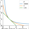
(a) Uniswap, Eq. 27

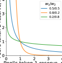
(b) Balancer, Eq. 36

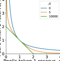
(c) Curve, Eq. 44

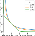
(d) DODO, Eq. 49

Figure 3. Conservation function (see §3.2.1) of amm with initial reserves of token₁ and token₂ both equal to 1, namely, ${\mathcal{K}}={\mathcal{R}_{1}}={\mathcal{R}_{2}}=1$.

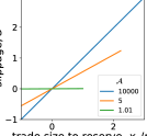
(a) Uniswap, Eq. 30

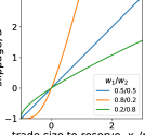
(b) Balancer, Eq. 39

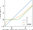
(c) Curve, Eq. 47

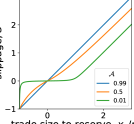
(d) DODO, Eq. 52

Figure 4. Slippage (see §3.2.4) of AMMs, depicted with $\frac{x_{1}}{r_{1}}\in[-1,3]$, corresponding to the after-trade token₁ reserve quantity $r_{1}\in[0,4]$, which is the x-axis of Fig. 3.

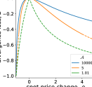
(a) Uniswap, Eq. 35

(b) Balancer, Eq. 43

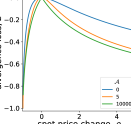
(c) Curve, Eq. 18

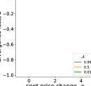
(d) DODO, $L\equiv 0$ at equilibrium

Figure 5. Divergence loss (see §3.2.5) of AMMs

4.1.1. Uniswap V2

The Uniswap protocol prescribes that a liquidity pool always consists of one pair of assets. Uniswap V2 implements a conservation function with a constant-product invariant (see §A.1.1), implying that the reserves of the two assets in the same pool always have equal value.

Liquidity provision or withdrawal at Uniswap V2 must be balanced and makes no price impact (§3.3.1). Swaps with Uniswap V2 are path-deterministic (§3.3.2); however, due to the positive swap fee charged and then immediately deposited back into the pool (Uniswap, 2022), a trading action can be decomposed into asset swap and liquidity provision. This action is, therefore, no longer a pure asset swap and would thus move the value of ${\mathcal{K}}$ (Senchenko, 2020). Uniswap V2 carries the properties of output-boundedness (§3.3.3), liquidity sensitivity (§3.3.4) and demand sensitivity (§3.3.5).

4.1.2. Uniswap V3

Uniswap V3 enhances Uniswap V2 by allowing liquidity provision to be concentrated on a fraction of the bonding curve (Adams et al., 2021) (see §A.2.1), thus virtually amplifying the conservation function invariant and reducing the slippage.

The protocol’s slippage controller $\mathcal{A}$ determines the degree of liquidity concentration. Specifically, $\mathcal{A}$ signifies how concentrated the liquidity should be provided around the initial spot price: when $\mathcal{A}\rightarrow\infty$, the covered price range approaches $(0,\infty)$, and the LP’s individual conservation function approximates a Uniswap V2 one (approximated with $\mathcal{A}=10000$ in 3(a)); on the other extreme, when $\mathcal{A}\rightarrow 1$, the liquidity only supports swaps close to the initial exchange rate, and the conservation function approximates a constant-sum one (3(a)).

Like V2, liquidity provision or withdrawal at Uniswap V3 must respect the existing ratio between two reserve assets, which results in zero price impact (§3.3.1). Different from V2 where fees are retained in the pool, Uniswap V3 deducts swap fees as a fraction of the input asset and credit that amount to lp’s fee revenue balance; hence, swaps with V3 are path deterministic with no impact on the bonding curve invariants (§3.3.2). By design, Uniswap V3 is not output-bounded (§3.3.3)—a sufficiently large swap can deplete one reserve asset and leave the liquidity pool only with the other one in (see 3(a)). Uniswap V3 also features liquidity sensitivity (§3.3.4). Thanks to its liquidity concentrating feature, Uniswap V3 is less demand sensitive (§3.3.5) than V2—a swap with a fixed input quantity would experience a lower slippage at Uniswap V3 than at V2 with the same level of pre-swap reserves (see 4(a)).

4.1.3. Balancer

The Balancer protocol allows each liquidity pool to have more than two assets (Martinelli and Mushegian, 2019). Each asset reserve $r_{k}$ is assigned a weight $w_{k}$ at pool creation, where $\sum\limits_{k}w_{k}=1$. Weights are pool hyperparameters and do not change with either liquidity provision/withdrawal or asset swap. The weight of an asset reserve represents the value of the reserve as a fraction of the pool value. Balancer can also be deemed a generalization of Uniswap; the latter is a special case of the former with $w_{1}=w_{2}=\frac{1}{2}$ for asset-pair pools (3(b)).

Balancer allows both balanced liquidity provision/withdrawal as well as single-asset liquidity change (Martinelli and Mushegian, 2019); the former does not cause price impact, whereas the latter does (§3.3.1). When only one asset is provided instead of e.g. eight, the protocol would first execute seven trades to swap this one asset to arrive at a vector of quantities in current proportions and next add this vector to the liquidity pool. Consequently, this sequence of actions is no longer a pure liquidity provision/withdrawal and would thus move the asset spot price. As Uniswap V2, swap fees with Balancer are also retained in the pool (Balancer, 2022), leading to an update of the bonding curve after each swap (§3.3.2). Balancer also features output-boundededness (§3.3.3), liquidity sensitivity (§3.3.4) and demand sensitivity (§3.3.5).

4.1.4. Curve

With the Curve protocol, formerly StableSwap (Egorov, 2019), a liquidity pool typically consists of two or more assets with the same peg, for example, USDC and DAI, or wBTC and renBTC. Curve approximates Uniswap V2 when its constant-sum component (§A.4.1) has a near-0 weight, i.e. $\mathcal{A}\rightarrow 0$ (3(c)).

Like Balancer, Curve allows both proportionate and disproportionate liquidity change to the pool, depending on which the lp’s action can induce either zero or some price impact (§3.3.1). As Uniswap V2 and Balancer, Curve updates its invariant after each trade to account for swap fees retained in the pool (§3.3.2). Curve is also output boundeded (§3.3.3), liquidity sensitive (§3.3.4) and demand sensitive (§3.3.5).

4.1.5. DODO

DODO supports customized pools (DODO, 2021b) where a pool creator provides reserves on both sides of the trading pair with arbitrary quantities, which determines the pool’s initial equilibrium state. Unlike conventional amm such as Uniswap, Balancer and Curve where the exchange rate between two assets in a pool is derived purely from the conservation function, DODO does it the other way around. Resorting to external market data as a major determinant of the exchange rate, DODO has its conservation function (see §A.5.2) derived from its exchange rate formula (see §A.5.1).

Specifically, the pool exhibits an arbitrage opportunity—namely a gap between the price offered by the pool and that from the external market—as soon as the reserve ratio between the two assets in the pool deviates from its equilibrium state. Price alignment by arbitrageurs always pulls the reserve ratio back to its equilibrium state set by the lp, thus eliminating any divergence loss. Due to this feature, DODO differentiates itself from other amm and terms their pricing algorithm as “pmm”, or pmm.

In DODO, a higher slippage controller $\mathcal{A}\in(0,1)$ results in a greater slippage around the market price—i.e. the equilibrium price. Specifically, when $\mathcal{A}\rightarrow 1$, the DODO bonding curve resembles Uniswap V2 (approximated with $\mathcal{A}=0.99$ in 3(d)); and with a high slippage around the market price (4(d)), the pool exhibits a strong tendency to fall back to the equilibrium state. When $\mathcal{A}\rightarrow 0$, the DODO bonding curve resembles a constant sum one (approximated with $\mathcal{A}=0.01$ in 3(d)); and with a near-flat slippage (4(d)), the algorithm’s force to pull the reserve ratio back to equilibrium is at its weakest due to little arbitrage profitability exhibited.

As with Balancer and Curve, lp can provide/withdraw both balanced and unbalanced reserves to a DODO pool (§3.3.1). Similar to Uniswap V3, swap fees with DODO are recorded outside of the liquidity pool. DODO’s bonding curve is thus redrawn not after each swap, but after each price change reported by the oracle (§3.3.2). DODO is also output boundeded (§3.3.3). Although relying on external price feeds for the construction of its conservation function, DODO is still liquidity sensitive (§3.3.4) and demand sensitivite (§3.3.5) since the size of a trade relative to the pool depth determines the magnitude of slippage and the price movement local to the pool.

4.1.6. Other amm-based dexs

Sushiswap

Sushiswap is a fork of Uniswap V2 (see §5.1.3). Though the two mainly differ in governance token structure and user experience, Sushiswap share the same conservation function, slippage and divergence loss functions as Uniswap.

Kyber Network

Currently in its 3.0 version, the dex uses a Dynamic Market Maker (DMM) mechanism, which allows for dynamic conservation functions based on amplified balances, called “virtual balances” (Krishnamachari et al., 2021). This is supposed to result in higher capital efficiency for lp and better slippage for traders. Also, the trading fees are adjusted automatically to market conditions. A volatile market causes increased fees, to offset impermanent loss for lp.

Bancor

While Bancor’s white paper (Hertzog et al., 2018) gives the impression that a different conservation function is applied, a closer inspection of their transaction history and smart contract leads to the conclusion that Bancor is using the same formula as Balancer (confirmed by a developer in the Bancor Discord community). As the majority of Bancor pools consist of two assets, one of which is usually BNT, with the reserve weights of 50%–50%, Bancor’s swap mechanism is equivalent to Uniswap. Bancor V2.1 now allows single-sided asset exposure, and provides divergence loss insurance (Bancor, 2020a) (see §4.2.3).

Summary

Each amm has its quirks. Uniswap V2 implements an rudimentary bonding curve that achieves a low gas fee; Uniswap V3 allows for concentrated liquidity provision which improves capital efficiency; Balancer supports more than 2 assets in a pool; Curve is suitable for swapping assets with the same peg; DODO proactively reduces divergence loss by leveraging external price feeds. As discussed in §4.1, common amm can be predominantly seen as a generalization, or an extension, of the most fundamental constant-product protocol that is applied by Uniswap V2.

When hyperparameters such as reserve weights $w_{k}$ and slippage controller $\mathcal{A}$ are assigned with certain values, various amm can be reduced to the basic form equivalent to Uniswap V2 (illustrated with blue curves in Fig. 3, 4 and 5). In fact, the majority of top amm—including Sushiswap, PancakeSwap, VVS Finance, Quickswap and BiSwap—are a simple clone of the Uniswap protocol (DefiLlama, 2022) with some adjustment in the fee and reward structure.

When deciding on a new conservation function, amm developers and designers must consider the trade-off between different features and properties (§3.3). For example, seeking liquidity insensitivity (§3.3.4) and demand insensitivity (§3.3.4) for low slippage leads to higher divergence loss (see §2.4.3): given a range of price movement, traders would be able to swap out an asset with a larger quantity, whereas lp would suffer a bigger divergence loss. In the extreme case like Uniswap V3, the trader-favoring feature sacrifices the output-bounded property (§3.3.3), which is to the detriment of lp, leaving them completely “rekt” in the case of significant price swings. Seemingly capable of achieving both low slippage and zero divergence loss at equilibrium by setting its $\mathcal{A}$ low, DODO appears to be an exception. Nevertheless, it is to be noted that with a small $\mathcal{A}$, DODO’s pmm algorithm is less effective in restoring the pool to its equilibrium state (see §4.1.5), thus still exposing lp to divergence loss risks in non-equilibrated states.

In a similar vein, users interacting with an amm-based dex, including both traders and lp, form a zero-sum game. They should understand the protocol design, and beware of embedded hidden costs such as slippage and divergence loss, which impose economic risks on their funds.

4.2. Additional features of amm-based dex

4.2.1. Time component

A time component refers to the ability to change traditionally fixed hyperparameters over time. Balancer V1 and V2 implement this (Table 3), by allowing liquidity pool creators to set a scheme that changes the weights of two pool assets over time. This implementation is called a Liquidity Bootstrapping Pool (see §4.3.4).

4.2.2. Dynamic swap fee

Dynamic fees are introduced by Kyber 3.0 to reduce the impact of divergence loss for lp. The idea is to increase swap fees in high-volume markets and reduce them in low-volume markets. This should result in more protection against divergence loss, as during periods of sharp token price movements during a high-volume market, lp absorb more fees. In low-volume and -volatility markets, trading is encouraged by lowering the fees.

4.2.3. Divergence loss insurance

Popularized by Bancor V2.1, lp are insured against divergence loss after 100 days in the pool, with a 30-day cliff at the beginning. Bancor achieves this by using an elastic BNT supply that allows the protocol to co-invest in pools and pay for the cost of impermanent loss with swap fees from its co-investments (Bancor Network, 2021). This insurance policy is earned over time, 1% each day that liquidity is staked in the pool.

Table 3. Overview of major existing amm-based dex on Ethereum, Solana, Polkadot, Tezos, EOS, Polygon and BNB Chain. CP: Constant product, CS: Constant sum, OP: Oracle price component, CC: Capital concentration, T: Time component.

			amm			amm add-ons
dex		Pool structure	CP	CS	OP	CC	T	Divergence loss compensation	Chain	Mainnet launch
Uniswap V1	(Adams, 2018)	asset-pair	●	○	○	○	○	—	Ethereum	11/2018
Uniswap V2	(Adams et al., 2020)	asset-pair	●	○	○	○	○	—	Ethereum	05/2020
Uniswap V3	(Adams et al., 2021)	asset-pair	●	○	○	●	○	—	Ethereum	05/2021
Balancer V1	(Martinelli and Mushegian, 2019)	multi-asset	●	○	○	○	●	—	Ethereum	03/2020
Balancer V2	(Martinelli, 2021)	multi-asset	●	○	○	○	●	—	Ethereum	—
Curve	(Egorov, 2019)	multi-asset	●	●	○	○	○	—	Ethereum	01/2020
DODO	(DODO Team, 2020)	various	●	○	●	○	○	—	Ethereum, BNB Chain	09/2020
Bancor V1	(Hertzog et al., 2018)	asset-pair	●	○	○	○	○	—	Ethereum, EOS	06/2017
Bancor V2	(Bancor, 2020a)	asset-pair	●	○	●	○	○	—	Ethereum, EOS	04/2020
Bancor V2.1	(Bancor, 2020b)	asset-pair	●	○	○	○	○	Divergence loss insurance	Ethereum, EOS	10/2020
SushiSwap	(Sushiswap, 2020)	asset-pair	●	○	○	○	○	—	Ethereum	08/2020
Mooniswap	(Bukov and Melnik, 2020)	asset-pair	●	○	○	○	●	—	Ethereum	08/2020
mStable	(Andersson, 2020)	asset-pair	○	●	○	○	○	—	Ethereum	07/2020
Kyber 3.0	(Kyber Network, 2021)	multi-asset	●	○	○	●	○	Dynamic swap fee	Ethereum, Tezos	03/2021
Saber	(Saber, 2021)	multi-asset	●	●	○	○	○	—	Solana	06/2021
HydraDX	(HydraDX, 2021)	multi-asset	●	○	●	●	○	—	Polkadot	—
Uranium Finance	(Uranium.finance, 2021)	asset-pair	●	○	○	○	○	—	BNB Chain	05/2021
QuickSwap	(QuickSwap Official, 2020)	asset-pair	●	○	○	○	○	—	Polygon	10/2020
Burgerswap	(Burgerswap, 2020)	asset-pair	●	○	○	○	○	—	BNB Chain	10/2020

4.3. Other defi protocols with amm implementations

amm form the basis of other defi applications (see Fig. 1) that implement existing or invent newly designed bonding curves, facilitating the functionalities of these implementing protocols. In this section, we present a few examples of projects that use amm designs under the hood.

4.3.1. Gyroscope

Gyroscope (Gyroscope Finance, 2021b) is a stablecoin backed by a reserve portfolio that tries to diversify defi tail risks. Gyro Dollars can be minted for a price near $1 and can be redeemed for around $1 in reserve assets, as determined through a new amm design that balances risk in the system. Gyroscope includes a Primary-market amm (P-amm), through which Gyro Dollars are minted and redeemed, and a Secondary-market amm (S-amm) for Gyro Dollar trading. Similar to Uniswap V3 where a price range constraint is imposed, the P-amm yields a mint quote and a redeem quote that serves as a price range constraint for the S-amm to decide upon concentrated liquidity ranges (Gyroscope Finance, 2021a).

4.3.2. EulerBeats

EulerBeats (EulerBeats, 2021) is a protocol that issues limited edition sets of algorithmically generated art and music, based on the Euler number and Euler totient function. The project uses self-designed bonding curves to calculate burn prices of music/art prints, depending on the existing supply. The project thus implements a form of amm to mint and burn NFTs price-efficiently.

4.3.3. Pods Finance

Pods (Pods Finance, 2021) is a decentralized non-custodial options protocol that allows users to create calls and or puts and trade them in the Options amm. Users can participate as sellers and buy puts and calls in a liquidity pool or act as lp in such a pool. The specific amm is one-sided and built to facilitate an initially illiquid options market and price option algorithmically using the Black-Scholes pricing model. Users can effectively earn fees by providing liquidity, even if the options are out-of-the-money, reducing the cost of hedging with options.

4.3.4. Balancer lbp

lbp are pools where controllers can change the parameters of the pool in controlled ways, unlike immutable pools described in §4. The idea of an lbp is to launch a token fairly, by setting up a two-token pool with a project token and a collateral token. The weights are initially set heavily in favor of the project token, then gradually “flip” to favor the collateral coin by the end of the sale. The sale can be calibrated to keep the price more or less steady (maximizing revenue) or declining to the desired minimum (e.g., the initial offering price) (Balancer, 2021).

4.3.5. YieldSpace

The YieldSpace paper (Niemerg et al., 2020) introduces an automated liquidity provision for fixed yield tokens. A formula called the “constant power sum invariant” incorporates time to maturity as input and ensures that the liquidity provision offers a constant interest rate—rather than price—for a given ratio of its reserves. fyTokens are synthetic tokens that are redeemable for a target asset after a fixed maturity date (Robinson and Niemerg, 2020). The price of a fyToken floats freely before maturity, and that price implies a particular interest rate for borrowing or lending that asset until the fyToken’s maturity. Standard amm protocols as discussed in §4 are capital-inefficient. By introducing the concept of a constant power sum formula, the writers want to build a liquidity provision formula that works in “yield space” instead of “price space”.

4.3.6. Notional Finance

Notional Finance (Notional Finance, 2021) is a protocol that facilitates fixed-rate, fixed-term crypto-asset lending and borrowing. Fixed interest rates provide certainty and minimize risk for market participants, making this an attractive protocol among volatile asset prices and yields in DeFi. Each liquidity pool in Notional refers to a maturity, holding fCash tokens attached to that date. For example, fDai tokens represent a fixed amount of DAI at a specific future date. The shape of the Notional amm follows a logit curve, to prevent high slippage in normal trading conditions. Three variables parameterize the AMM: the scalar, the anchor, and the liquidity fee (Notional Finance, 2020). The first and second mentioned allowing for variation in the steepness of the curve and its position in a xy-plane, respectively. By converting the scalar and liquidity fee to a function of time to maturity, fees are not increasingly punitive when approaching maturity.

4.3.7. Gnosis cmm

The Gnosis cmm (Gnosis, 2020) allows users to set multiple limit orders at custom price brackets and passively provide liquidity on the Gnosis Protocol. The mechanism used is similar to the Uniswap V3 structure, although it allows for even more possibilities to market makers by allowing them to choose price upper and lower limits and a number of brackets within that price range. Uniswap V3 allows lp to solely choose the upper and lower limits. Because users deposit funds to the assets at different price levels specifically, the protocol behaves more like a central limit order book than an amm pool.

4.3.8. dex aggregators

dex aggregators are a type of emerging defi protocols that connect to various other dex and can also have their own liquidity pools (Ushida and Angel, 2021). They offer traders superior swap rates through routing across liquidity pools from different dex with one single user interface (Raikwar and Gligoroski, 2021). 1inch and Paraswap are two major dex aggregators for evm-compatible chains that incorporate amm such as Uniswap and Curve. Rango (Rango, 2022) is an example of cross-chain dex aggregators incorporate amm, dex aggregators and bridges to facilitate token swaps across both evm and non-evm blockchains.

4.4. amm on Layer 2 solutions

The growth and success of defi on Ethereum have put a strain on the Ethereum network’s ability to process transactions, leading to increasing gas (YCharts, 2021). As the Ethereum Network becomes busier, user experience decreases because of increasing gas prices and decreasing transaction speed. Users aim to outbid each other by increasing the gas prices. Also, transaction speed decreases, which results in poor user experience for certain types of dapp. And as the network gets busier, gas prices increase as transaction senders aim to outbid each other. In an attempt to prevent these consequences, “layer 2 solutions” (L2) are being developed. These solutions handle transactions outside of the Ethereum network, but still rely on the decentralized security model of the mainnet (ethereum.org, 2021a). Examples of layer 2 technologies include Plasma, Sidechains, Optimistic Rollups and ZK-Rollups. For a more comprehensive reading on this topic, we direct the reader to (ethereum.org, 2021b). Examples of Ethereum layer 2 solutions are Polygon (Polygon, 2021), Arbitrum (Arbitrum, 2021), Optimism (Optimism, 2021) and Starknet (StarkWare Industries Ltd., 2021).

Characteristics of layer 2 solutions, such scaling and security, have been well-documented across different sources (Gudgeon et al., 2020a) (Hafid et al., 2020) (Jourenko et al., 2019) and are out of scope for this sok. The advantages and disadvantages of transacting on layer 2 solutions are not specifically related to amm, but to all protocols on these technologies. Therefore, we focus on the security issues and user experience of interacting with amm on layer 2.

Daian et al. (Daian et al., 2020) note that abstraction achieved by layer 2 exchange systems is not sufficient to prevent sandwich attacks and a report of Delphi Digital (Delphi Digital, 2020) concludes that there is still front-running risk when a protocol wants to aggregate liquidity across layer 1 and layer 2 pools. The front-running and sandwich attacks does not seem to be solved by layer 2 solutions. (Konstantopoulos, 2021) proposes a simple solution for front-running attacks on Optimistic Rollups technology.

One of the most important advantages of deploying a protocol on layer 2 is the reduction in gas fees. This dramatically enhances the user experience, and opens up ways to introduce new forms of decentralized exchanges. One example is ZKSwap (ZKSwap, 2021), allowing users to trade with zero gas fees. Sushiswap and Curve have deployed their contracts on Polygon and QuickSwap is a fork of Uniswap on that same layer 2 solution (Nasdaq, 2021). As a result, users are now able to use the same products on layer 2 solutions, with drastically reduces costs and allows faster transactions. In 2021, dYdX launched its order book-based dex on StarkEx (dYdX, 2021).

In sum, amm on layer 2 solutions result in faster transactions and a reduction of costs due to zero or decreased gas costs, ultimately enhancing the user experience.

5. Security and privacy concerns

The previous sections focus on implicit economic costs—including slippage and divergence loss—imposed on the funds of users interacting with amm-based dex. Besides those risks, security and privacy matters are also to be taken into account when using amm-based dex.

In particular, as a complex, distributed system with a variety of software and hardware components interacting with each other, amm-based dex are prone to exhibit attack interfaces (Li et al., 2020; Lin and Liao, 2017; Zhang et al., 2019; Massacci and Ngo, 2021). With conventional exchanges, the success of market manipulation is uncertain as each trade must be agreed upon between the sell and buy sides. In contrast, amm-based dex are subject to atomic, risk-free exploits on the protocol’s technical structure such as its algorithmic pricing scheme (Sam M. Werner et al., 2022). Built on top of public blockchain infrastructures featuring transparency and traceability, amm-based dex also expose their users to privacy risks.

In this section, we define a taxonomy (illustrated in Fig. 6) to enumerate potential security and privacy concerns of amm-based dex, expounding their root causes and possible mitigation solutions.

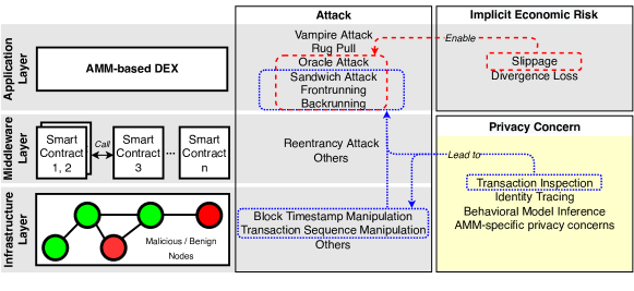
Figure 6. Architectural layers of an amm-based dex with its implicit economic risks, attacks, privacy concerns, and their relationships.

5.1. Associated attacks

We identify three classes of attacks according to the architectural layer on which they occur: infrastructure-layer attacks, middleware-layer attacks, and application-layer attacks. Sometimes, a certain attack (e.g. frontrunning) can target multiple layers simultaneously. We present known historical attacks affecting amm in Table 5.

5.1.1. Infrastructure-layer attacks

The proper operation of dex are based upon healthy and stable blockchain infrastructures (i.e., validators, network, full nodes, etc.). However, since the birth of the blockchain systems, various attacks have threatened their normal operations, potentially affecting the robustness and user experience of dex.

Block timestamp manipulation

A timestamp field is set by miners during the validation process. However, malicious miners can manipulate the block timestamps within constraints to win rewards from certain smart contracts (Crypto Market Pool, 2020), or to tamper with the execution order of dex transactions packed in different blocks (Huang, 2019).

To mitigate the negative impact of such manipulation, dex contracts should be timestamp independent (Antonopoulos and Wood, 2018). For example, smart contract engineers should avoid using block timestamps as program inputs or make sure a contract function can tolerate variations by a certain time period (e.g. 15 seconds (Narayanan et al., 2016)) and still maintain integrity (Mense and Flatscher, 2018). Besides, dex should choose to be built on a blockchain that applies rigorous constraints to the timestamps of committed blocks or uses external timestamp authorities to assert a block creation time (Szalachowski, 2018).

Transaction sequence manipulation

While transactions within a block share the same timestamp, miners can order transactions, and choose to include or exclude certain transactions at their discretion. Malicious miners can abuse their “power” to prioritize transactions in their favor, profiting from the mev, which is the value that is extractable by miners directly from smart contracts during the validation or mining process (Zhou et al., 2021b; Qin et al., 2022) This can be further facilitated by open-source software such as Flashbots (Daian et al., 2020).

To prevent transaction sequence manipulation, dex should first be built upon reputable, frequently-used blockchain systems, as they feature high miner/validator participation, making transaction sequence manipulation difficult. Besides, this attack can be mitigated through an enforced transaction sequencing rule that relies on a trusted third party to assign sequential numbers to transactions (Eskandari et al., 2020). We also discuss how dex and their transactions can practice transaction sequencing from application-layer in §5.1.3, and how privacy-preserving blockchain and dex are resistant to this attack in §5.2.

Other infrastructure-layer attacks

Aiming to perturb operations of blockchain systems (Saad et al., 2019), many other attacks do not target amm-based dex specifically, but can indirectly affect the service of dex. For example, attackers can launch spam or ddos attacks towards the blockchain system (Greene and Johnstone, 2018; Perez et al., 2020), thereby increasing the latency or even hindering the accessibility of dex services; bdos attacks exploit the reward mechanism to discourage miner participation, thereby causing a blockchain to a halt with significantly fewer resources (Mirkin et al., 2020); the 51% attack (Saad et al., 2019), the most classic blockchain attack, is able to tamper with the blockchain in any way by controlling more than 50% of the network’s mining hash rate; network attacks can destroy the network connections between the users and the blockchain system through dns hijacking (Ramdas and Muthukrishnan, 2019) or bgp hijacking (Apostolaki et al., 2017).

In short, amm-based dex should be built upon distributed ledgers with active service, community maintenance, and upgrades, as well as modular security designs. Only by ensuring each module of the blockchain system and the interactions between them are secure, can the relative security of the entire blockchain system be ensured.

5.1.2. Middleware-layer attacks

An amm-based dex usually consists of various smart contracts, in which each serves as a middleware that bridges some application-layer functions with blockchain infrastructures, and collectively support operations of dex. However, the smart contracts and complex collaborations between them can also lead to potential system vulnerabilities (Tsankov et al., 2018). Attackers can exploit such attack interfaces to steal tokens from a dex or even paralyze it.

Reentrancy attack

Reentrancy attack can happen when two or more entities (e.g. smart contract, side-chain) call or execute certain functions in specific sequences or frequencies. Ever since July 2016, reentrancy attacks have captured the attention of the crypto industry, when the dao, an Ethereum smart contract, was executed maliciously with such an attack, causing a $50 million economic loss in tokens (Popper and Nathaniel Popper, 2016). Afterwards, despite the emergence of various proposals addressing the reentrancy problems (Luu et al., 2016; Tsankov et al., 2018; Albert et al., 2020), reentrancy attacks persist, and became particularly threatening to amm-based dex. In January 2019, an audit identified a reentrancy vulnerability in Uniswap (Consensys Diligence, 2019), which was then exploited by hackers to steal $25 million worth of tokens in April 2020 (PeckShield, 2020a) Hackers performed this attack by leveraging a subtle interaction between two contracts that were secure in isolation, and a third malicious contract (Cecchetti et al., 2021). In March 2021, $3.8 million worth of tokens were stolen from DODO through a series of attacks, which began with reentrancies via the init() function in a liquidity pool smart contract, followed by frontrunning and honeypot attacks (DODO, 2021a).

The security community has proposed a variety of approaches to tackle reentrancy attacks (Huang et al., 2019). For example, Rodler et al. (Rodler et al., 2019) protect existing smart contracts on Ethereum in a backwards compatible way based on run-time monitoring and validation; Das et al. (Das et al., 2021) propose Nomos, a reentrancy-aware language that enforces security using resource-aware session types; Cecchetti et al. (Cecchetti et al., 2021) formalize a general definition of reentrancy and leverage information flow control to solve this problem in general. However, with the increasing complexity of amm, it can become more difficult for developers to reason about the reentrant interface, thus making reentrancy attacks a more intractable problem for amm-based dex.

Other middleware-layer attacks

On the middleware layer, there are many other attacks and threats that can affect normal operations of smart contracts (Sayeed et al., 2020), such as replay attack (Ramanan et al., 2021), exception mishandling (Praitheeshan et al., 2019), integer underflow/overflow attacks (Sun et al., 2021), etc. These threats are not specifically targeted at dex, but can potentially be harmful to dex operation. The security community has proposed a variety of approaches to secure smart contract from these threats, such as Smartshield (Zhang et al., 2020a), Zether (Bünz et al., 2020), and NeuCheck (Lu et al., 2019). Users may also purchase insurance cover to hedge smart contract risks (Cousaert et al., 2022a). To fundamentally counter those attacks, smart contract coders must strictly abide by software development specifications and conduct thorough security tests.

5.1.3. Application-layer attacks

Oracle attack

A flash loan is a feature provided by lending platforms where an uncollateralized borrow position can be created as long as the borrowed funds can be repaid within one transaction (Xu and Vadgama, 2022). Flash loans can be used to repay at discount debts that are liquidable without having to acquire borrowed assets in the first place. In this kind of attack, adversaries manipulate lending platforms that use a dex as their sole price oracle (see Fig. 1).

Following Attack Algorithm 1, an attacker profits with $\Delta_{3}$ token_A less any transaction fees incurred. Utilizing continuous slippage native to an amm-based dex (see §3.2.4), the attack temporarily distorts the price of token_A relative to token_B. After the prices are arbitraged back, the attack would leave the loan taken from step 3 undercollateralized, jeopardizing the safety of lenders’ funds on the lending platform. Examples of such attacks are exploits on Harvest finance (Harvest Finance, 2020), Value DeFi (PeckShield, 2020b) and Cheese bank (Pirus, 2020).

This broken design can generally be fixed by either providing time-weighted price feeds, or using external decentralized oracles. The first solution ensures that a price feed cannot be manipulated within the same block, while the second solution aggregates price data from multiple independent data providers that add a layer of security behind the aggregation algorithm, making sure that prices are not easily manipulated (SmartContent, 2021).

Rug pull

A rug pull involves the abandonment of a project by the project foundation after collecting investor’s funds (Xia et al., 2021). One way of doing this, is to lure people into buying the coin with no value through a dex, subsequently swapping this coin for ETH or another cryptocurrency with value, as shown in Attack Algorithm 2. dex allow users to deploy markets without audit and for free (barring the gas costs), which makes them an excellent target to scam investors. One method is to create a coin with the same name as an existing one. This attracts a lot of attention since everyone wants to pick up the coin at the lowest price possible. The coin is being bought up, and the original lp swaps his fake coin for ETH. In other cases, the creators of the scam token reach out to several prominent people, creating false hype. Once potential buyers see that major players have purchased the token, they start buying themselves, before realizing that the token cannot be swapped back for ETH. Sometimes, the attackers let people trade the coin back for ETH, but only for a short period since they are running the risk of losing money. (Xia et al., 2021) research data on scam tokens on Uniswap and confirm that rug pulls commonly find their victims through dex.

In August 2020, an rug puller extracted 3 ETH by imitating the well-known AMPL token (Ampleforth, 2021) with a scam token TMPL. The token’s transaction history shows the provision of 150 ETH and TMPL tokens to a Uniswap V2 pool by the attacker, who removed 153.81 ETH only 35 minutes later (Etherscan, 2021).

To protect themselves from being rugged, investors should exercise caution and always confirm a project’s credibility before investing in its ido (Bybit Learn, 2021; The European Business Review, 2021). Usually, reputable ido feature high liquidity and a pool lock (rug, 2021) that disables withdrawal for a fixed period, so that lp are unable to quickly empty the pool once it has absorbed a sufficient amount of valuable assets from investors (Mudra Manager, 2021).

Frontrunning

Frontrunning is often enabled through access to privileged market information about upcoming transactions and trades (Eskandari et al., 2020). Since all transactions are visible for a very short period of time before being committed to a block, it is possible for a user to observe and react to a transaction while it is still in the mempool. Those who place their trade immediately before someone else’s are called frontrunners (Daian et al., 2020; Eskandari et al., 2020). Frontrunners attempt to get the best price of a new coin before selling them onto the market. They can buy up a great portion of the supply of a new token to create exorbitant prices. Due to the hype, this does not stop retail traders from further buying. The frontrunner, who is the seller with the most significant supply, can swap the purchased token for popular coins (e.g. ETH) paid by retail traders. For example, a considerable amount of ido on Polkastarter are frontran on Uniswap (Taylor, 2021).

Frontrunning can also be achieved through transaction sequence manipulation (see §5.1.1) and by exploiting the general mining mechanism. Most mining software, including the vanilla Go-Ethereum (geth), the most popular command-line interface for running Ethereum node, sorts transactions based on their gas price and nonce (Zhou et al., 2021c; Eskandari et al., 2020; Daian et al., 2020). This feature can be exploited by malicious users of dex who broadcast a transaction with a higher gas price than the target one to distort transaction ordering and thus achieve frontrunning.

Frontrunning can be avoided with various approaches (Baum et al., 2021a). Normal exchange users can set a low slippage tolerance to avoid suffering from a price elevated by front-runners. However, an overly low slippage tolerance may lead a transaction to fail, especially when the trade size is large, resulting in a waste of gas fee (Degate, 2021). dex can enforce transaction sequencing to fundamentally solve frontrunning. Some exchanges, such as EtherDelta (Narayanan et al., 2016) and 0xProject (Warren and Bandeali, 2017), utilize centralized time-sensitive functionalities in off-chain order books (Eskandari et al., 2020). In addition, transactions can specify the sequence by including the current state of the contract as the only state to execute on (Eskandari et al., 2020), thereby preventing some types of frontrunning attacks. Frontrunning can further be tackled by addressing privacy issues (see §5.2) and transaction sequence manipulation on the infrastructure layer (see §5.1.1).

Backrunning

Backrunners place their trade immediately after someone else’s trade. The attacker needs to fill up the block with a large number of cheap gas transactions to definitively follow the target’s transaction. Compared to frontrunning which only requires a single high valued transaction and is detrimental to the user being frontrun, backrunning is disastrous to the whole network by hindering the throughput with useless transactions (livnev, 2020).

Backrunning attacks can be mitigated through anti-bdos solutions such as A²MM (Zhou et al., 2021a). Theoretically, defense solutions of l7ddos attacks (Feng et al., 2020; Xie and Yu, 2008; Wang et al., 2017) can also be adopted to tackle backrunning problems, as they all aim to secure usability of web services to legitimate users. In addition, backrunning can be addressed by confidentiality-enhancing solutions that hide the content of a transaction before it is committed to a block (see §5.2).

Sandwich attacks

Combining front- and back-running, an adversary of a sandwich attack places his orders immediately before and after the victim’s trade transaction. The attacker uses front-running to cause victim losses, and then uses back-running to pocket benefits. While there are endless examples of sandwich attacks, Zhou et al. (Zhou et al., 2021c) detail two types that can occur on an amm: an lp attacking an exchange user (see Attack Algorithm 3) by exploiting amm’s liquidity sensitive property (§3.3.4), and one exchange user attacking another (see Attack Algorithm 4) by taking advantage of amm’s demand sensitive property (§3.3.5). The latter is particularly common. Fig. 7 shows two examples of such attacks on Uniswap V2 within a time frame of 3 minutes.

Figure 7. Two sandwich price attacks (see Attack Algorithm 4), marked with orange ◻ on 30/09/2021, with the STARL/ETH pair on Uniswap V2. The attack conducted at 10:16:46 by 0xa405e8…f802 resulted in a profit of 0.0310743 ETH; the attack conducted at 10:19:52 by 0x1d6e8b…932d resulted in a profit of 0.0308927 ETH.

Considering swap fee (see §2.4.2), gas fee (see §2.4.2) and slippage (see §2.4.3), sandwich attacks are only profitable if the size of the target trade exceeds a certain threshold, a value that depends on the dex’s design and the pool size. dex can thus prevent sandwich attacks by disallowing transactions above the threshold (Zhou et al., 2021a). Naturally, sandwich attacks can also be curbed by deterring either frontrunning (see §5.1.3) or backrunning (see §5.1.3).

Vampire attack

A vampire attack targets an amm by creating a more attractive incentive scheme for lp, thereby siphoning out liquidity from the target amm (Jakub, 2020) to the detriment of the protocol foundation (see §2.1.3). In September 2020, Sushiswap gained $830 million of liquidity through a vampire attack (Dale, 2020), where Sushiswap users were incentivized to provide Uniswap lp tokens into the Sushiswap protocol for rewards in SUSHI tokens (Sushiswap, 2020). A migration of liquidity from Uniswap to protocol Sushiswap was executed by a smart contract that took the Uniswap lp tokens deposited in Sushiswap, redeeming them for liquidity on Uniswap which was then transferred to Sushiswap and converted to Sushiswap lp tokens.

Legal approaches such as applying a restrictive license to the protocol code base—as done later by Uniswap with its V3 new release (Foxley, 2021a)—can be employed to hinder vampire attacks.

5.2. Privacy concerns

Most blockchain systems are open, traceable, and transparent, which can raise severe privacy concerns to dex that built upon them. Besides, amm protocols will reveal real-time dex information to the public, bringing additional privacy concerns to amm-based dex. In this section, we introduce the privacy issues that users may face in using amm-based dex and discuss their possible solutions.

5.2.1. Transaction inspection

The transparency and openness of public blockchains, where most amm-based dex are built, allow transactions to be observable to everyone. However, this characteristic enables malicious parties to inspect transactions, thereby seeking profits or even disrupting the market (Eskandari et al., 2020). The inspection activities can occur before or at the moment that the transaction is committed to the blockchain by miners, validators, or even any third parties. For example, the aforementioned frontrunning, backrunning, sandwich attacks, transaction sequence manipulation, and block timestamp manipulation in Section 5.1 are all based on transaction inspections (Goldreich and Oren, 1994). In fact, major amm-based dex are fraught with bots, constantly monitoring transactions for possible profit opportunities (Narayanan et al., 2016).

5.2.2. Identity tracing

Although most blockchains and amm-based dex usually feature a certain degree of anonymity, the linkabilities of transactions and accounts over time still enable attackers to dig identities information of users (Zhang et al., 2019). Actually, with some off-chain information (e.g. social network posts, public speak, location (DuPont and Squicciarini, 2015)), eavesdroppers can launch de-anonymization inference attacks to bridge virtual accounts with real-world individuals or uncover the true identities of traders by linking the transactions of an account together and matching relevant information (Narayanan et al., 2016).

5.2.3. Behavioral model inference

By collecting data from corresponding blocks and analyzing historical transactions of an account, any third parties infer an account’s behavioral model, understanding its active phase, trading frequency, or even preferences. Such activity is called behavioral model inference, which not only compromises user privacy, but can also make preparations for launching honeypot attacks (Qin et al., 2022) and phishing scams (Xia et al., 2021; Chen et al., 2020a; Phillips and Wilder, 2020; Wu et al., 2020).

5.2.4. amm-specific privacy concerns

While it is possible to anable privacy-preservance with non-amm-based dex (Govindarajan et al., 2022; Baum et al., 2021b) by hiding all the information such as the transaction, order book, and trading volume, it is challenging to make amm-based dex fully privacy-preserving. Due to their path-deterministic property (see §3.3.2), information on swaps with an amm pool is often reverse-engineerable (Angeris et al., 2021c). Some researchers even argue that complete privacy is impossible once dex apply ordinary implementations of cfmm (e.g., Uniswap, Balancer, Curve, etc.) under reasonable adversarial models (Angeris et al., 2021b). The transparency and openness allow any third party to capture rich data about the amm-based dex, such as the overall trading situation per block, asset pool changes over time, or popular tokens on the platform. Under this circumstance, even though the dex can hide the detailed information about a transaction, we can still estimate the transaction amount and transaction currencies according to the amm protocols.

Solution

The confidentiality of amm-based dex’s pipeline can be enhanced from various angles to limit public access to certain information. Such information includes but is not limited to the transaction amount, asset type, user/pool balance, user identification, order of transactions, mev, or protocol-related information. Hiding all the information from both the public and computation parties can fundamentally resolve the privacy concerns, thereby eliminating all the associated attacks and privacy disclosure. However, it may break the market visibility to traders, cause difficulties to governance and regulation, and make the whole system inefficient to operate. On the other hand, achieving partial confidentiality may be sufficient to prevent many attacks and provide enough privacy protections to traders. Thus, most existing solutions focus on enhancing the user privacy of certain components in amm-based dex.

On the infrastructure layer, many privacy-preserving blockchain solutions have been proposed to increase confidentiality (Bünz et al., 2018; Bernabe et al., 2019) and anonymity (Miers et al., 2013; Noether, 2015; Sasson et al., 2014) for transactions. These solutions can be based on zkp (Goldreich and Oren, 1994), homomorphic encryption (Gentry, 2009), or identity obfuscation (Goldwasser and Rothblum, 2007), aiming to break the linkability of transactions, encrypt transaction content, or anonymize users accounts. amm-based dex built upon these blockchains not only can protect user privacy, but also can defend against attacks discussed in §5.1.1 and §5.1.3. Besides, developers can choose to leverage pbs (vbuterin, 2022) to hide transaction details from miners or validators. Although pbs can only achieve miner/validator-specific privacy, it can increase the censorship resistance of transactions against miners and validators, thereby defending against frontrunning attacks effectively and efficiently. Ferveo (Bebel and Ojha, 2022) is a similar approach, which is a fast protocol for Mempool Privacy to avoid transaction censorship.

Even though the blockchain infrastructures are transparent, confidentiality can be achieved through privacy designs on upper layers. On the middleware layer, developers can leverage techniques such as Hawk (Kosba et al., 2016), Ekiden (Cheng et al., 2019), and Submarine Commitments (Breidenbach et al., 2018) to develop privacy-enhanced smart contracts for amm-based dex. On the application layer, privacy-enhanced dex are proposed to resolve the privacy concerns. For example, P2DEX (Baum et al., 2021b) harnesses mpc (Cramer et al., 2015) to realize efficient privacy-preserving dex; ZKSwap (ZKSwap, 2021), an amm-based dex utilizing ZK-Rollup (Gluchowski, 2019) technology, not only provides users with extra privacy protections when withdrawal, deposit, and transfer of tokens by leveraging zkp, but also significantly reduce gas fees for transactions; ZEXE (Bowe et al., 2020), a ledger-based system that enables users to realize privacy-preserving analogues of popular applications, such as dex. ZEXE can make it easy to satisfy two main privacy properties. First, transactions hide all information about the offline computations. Second, transactions can be validated in constant time by anyone, regardless of the offline computation; Zswap (Engelmann et al., 2022), a zk-SNARKs-based transaction scheme that enables multiple assets and atomic exchanges with sparse homomorphic commitments and Zcash friendly simulation-extractable nizk proofs.

Furthermore, on-chain privacy-preserving services and products are on the rise. For example, Blank (Blank, 2021), a non-custodial Ethereum browser extension wallet, offers transaction obfuscation; Enigma (Kisagun, 2019) builds a network of “secret nodes” that can perform computations on encrypted data without the necessity to expose original raw data.

However, as mentioned above, even details of an individual transaction will not be disclosed, it is still possible to infer rough information of transactions through the asset pool state changes and amm protocols (Angeris et al., 2021b). As the amm protocols and asset pool state should be accessible to the public, any third party can keep tracking the asset pool changes and then deduce how many assets and which assets were traded during each block. From the perspective of computation parties (i.e., miner), they can fetch even more granular pool state changes to infer detailed transaction information in the mempool. Hence, most existing privacy-preserved dex designs are hardly compatible with amm protocols. To overcome this problem, developers can use non-constant function market makers or apply fuzzification to conservation functions. However, this will also bring some side effects to traders, as it can incur larger slippages to the final trading prices. In addition, privacy-enhanced amm-based dex can increase the difficulty of market supervision, creating obstacles for governance, regulation, and financial control. Therefore, how to reach a balance between privacy protection and policy compliance is a question worth exploring for the entire crypto industry.

6. Avenues of future research

While dex with amm protocols are maturing, there still exists room for further development, expansion, and exploration. In this section, according to existing literature, our observations about recent trends, and major problems to be solved in this field, we discuss avenues for future research from the perspectives of security, privacy, system design, protocol design, and governance. Fig. 8 shows a graphical illustration of future research avenues.

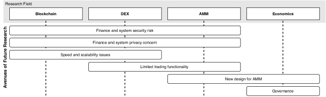
Figure 8. A graphical illustration of future research avenues.

6.1. Finance and system security risk

Compared with order-book-based dex, an amm-based dex leverages bonding curves to determine asset prices without reaching any agreements between buyers and sellers. However, this feature can also bring severe security risks and leave many unsolved problems. For example, once attackers successfully manipulate the asset prices in amm-based dex, they can theoretically drain all the associated assets from the asset pool, causing severe damage to the trading market. This matter is worthy of deep investigation in the future.

In addition, as a nascent type of trading platforms built on complicated distributed systems (i.e., blockchain), amm-based dex operate upon various components run by many different parties. Therefore, any flaws in this system can pose threats to the trading market, potentially causing both economic losses and system dysfunction. As discussed in §5, in recent years, amm-based dex suffered from a variety of attacks for different reasons, such as oracle attacks caused by flaws of oracle components in blockchains, vampire attacks caused by the lack of market regulation, flash loan attacks caused by unsound trading rules, and reentrancy attacks caused by inappropriate function calls of smart contracts. Patching those vulnerabilities without bringing significant changes to existing systems requires joint efforts from both computer science, economics, and finance researchers.

6.2. Finance and system privacy concern

Privacy is another major concern in amm-based dex (§5.2). At present, most dex systems are built on top of public blockchains such as Ethereum to record transactions in plain text, which enables everyone to observe detailed transactional information. An attacker could inspect an amm protocol, access the associated transactions from the blockchain, and launch attacks such as frontrunning, backrunning, and sandwich attacks. Even most blockchain systems provide a certain degree of anonymity (i.e. pseudonymous), recent studies have shown that deanonymization attacks can link transactions to users’ accounts and reveal users’ real identities. Besides, the AMM algorithm itself can leak rich information about the dex, enabling any third parties to estimate the detailed transaction information.

As discussed in §5.2, some general solutions such as Zerocash (Sasson et al., 2014), Hawk (Kosba et al., 2016), and ZEXE (Bowe et al., 2020) have been proposed to achieve ledger privacy in dex. However, they would substantially decrease the real-time efficiency in amm-based dex, thereby very expensive to deploy in amm-based dex. Researchers can try to optimize the system design and the cryptographic algorithm efficiency of those approaches, thus preserving the swap velocity while enhancing user privacy. In addition, existing privacy-preserving blockchains and dex are not compatible with amm protocols. Even transaction information is protected on blockchains, people can still deduce the transaction’s asset type and exchange amount from asset pool transformations. Therefore, a new amm-oriented dex that can preserve user privacy at certain degrees is worthy of study. Possible research directions include adding stochasticity to the amm protocol, developing non-constant function market makers, or applying fuzzification to current amm. Moreover, existing privacy solutions could also result in governance issues; since these solutions provide full privacy for transactions, it is almost impossible for law enforcement to investigate cryptocurrency-related crimes in dex such as theft, money laundering, and illegal transactions in dark markets. Finally, introducing privacy in amm-based dex may affect asset prices, asset liquidity, and market predictability across different markets, thus requiring new economic models and protocols to analyze the reward and cost for amm economics.

6.3. Speed and scalability issues

As amm-based dex operate on top of blockchain systems, their transaction speed and scalability are limited by the growth speed and throughput of the blockchain networks.

On the one hand, each dex transaction takes time to be validated on the blockchain network before it takes effect. The validation speed depends on the miners or validators, rather than the dex. Compared with centralized exchanges that will immediately finishing processing user transactions, dex will incur a processing delay ranging from a couple of seconds to several hours. Although some blockchain networks are specifically designed for velocity requirements (e.g., Tezos, XRPL, EOSIO, etc.), their delays are still measured in seconds (Perez et al., 2020).

On the other hand, as the information of dex transactions must be recorded in blocks, the total number of transactions that a dex can accept per batch is limited. Although many multi-layer blockchains (e.g., layer 2 blockchains) were proposed to resolve the throughput issue (Sguanci et al., 2021), their throughput is still an order of magnitude behind centralized exchanges.

Therefore, a vital future research direction is to keep improving the validation speed and throughput of blockchain systems, thereby increasing the speed and scalability of the amm-based dex built upon them. Resolving this issue not only can scale amm-based dex to a large group of users, but also can ensure that each transaction can be processed timely. New types of data structure, synchronization mechanism, or validation approaches should be proposed to conquer this problem.

6.4. Limited trading functionality

Compared to centralized exchanges nowadays, the trading functionalities of amm-based dex are limited to buying and selling. Due to the nature of amm-based dex, the lacks of stop-loss ability, margin trading, and put and call options greatly restrict users’ financial operations on the platforms. Besides, it is difficult to implement additional functionalities to existing amm protocols.

To enhance the trading functionality of amm-based dex, researchers need to bring some structural changes to currently amm-based dex. For example, researchers can try to bridge amm and order book to provide put and call options; leveraging smart-contract-based lending can also help amm-based dex to provide trading margins to users.

6.5. New design for amm

We find that the majority of amm-based dex use a cfmm algorithm that can be seen as a variation of Uniswap’s constant product protocol. It would be worth exploring novel bonding curves or new amm designs that can, e.g., balance slippage and impermanent loss in different ways.

Current amm implementation can be mainly seen with dex for spot markets. While still at its infancy, dex for financial derivative markets have also been witnessing an increase in the adoption of amm algorithms, such as Siren (Siren, 2021) and Hegic (Wintermute, 2020) for options, the Perpetual Protocol for perpetual contracts (Perpetual Protocol, 2021), and Tracer (Garner et al., 2021) for swaps. As those protocols are still at their early development phase, they have not been thoroughly tested by the market or scrutinized by academia. As the derivative dex using amm become more mature, it would be of scholars’ and practitioners’ interest to see a systematization of these protocols and an investigation on how they advance from the basic amm for spot markets.

6.6. Governance

Due to its decentralized and censorship-resistant nature, dex participants have the liberty to do whatever is permissible by the smart contract code, sowing the seeds for malicious and fraudulent behavior. In such context, governance schemes are essential to ensure the proper operation of amm-based dex. However, centralization of voting power is frequently observable with amm-based dex due to the often concentrated nature of protocol token distribution. Furthermore, regulatory concerns often go hand in hand with governance issues. For example, the Uniswap community has been debating whether or not to turn the fee switch on for the UNI buyback program (Uniswap Governance, 2021). In fear of legal consequences in the case of UNI being categorized as a security token, the protocol has yet to enable the function due to its similarity to a regular stock buyback exercise, leaving the UNI token value unbacked by any monetary flow.

Whether and how the governance mechanism can be improved for more sustainable development of a protocol in a legally compliant way thus merit further research.

7. Related work

In Table 6, we summarize most sok, surveys and tutorials that investigate the dapp ecosystem on blockchain. Our work differs from those existing works in the following aspects:

1. we have a clear, focused study subject: dex-based amm, while the majority of related survey studies either examines other defi applications (e.g. lending protocols (Bartoletti et al., 2021a), yield aggregators (Cousaert et al., 2022b; Xu and Feng, 2022)) or have a broader coverage;

2. we use a comprehensive set of methods to generalize and systematize dex-based amm protocols, including taxonomization, state space modeling, numerical simulation and empirical investigation, while most existing related survey studies use only a subset of the aforementioned methods;

3. we examine an array of aspects of dex-based amm, including their architectural design and internal mechanism, financial economics as well as as associated security and privacy concerns, while most of the related survey papers only cover some of these aspects.

In the following, we discuss more literature related to our study in various ways.

7.1. AMM-based DEX on blockchain

Our work is first and foremost related to the literature body covering amm-based dex on blockchain.

7.1.1. Protocol mechanism

Angeris et al. (Angeris et al., 2021a) discuss arbitrage behavior and price stability in constant product and constant mean markets. Lo et al. (Lo and Medda, 2020) empirically evidence that the simplicity of Uniswap ensures the ratio of reserves to match the trading pair price. Despite historical oracle attacks associated with amm (see §5), Angeris et al. (Angeris et al., 2021a; Angeris and Chitra, 2020) show that cfmm users are incentivized to correctly report the price of an asset, suggesting the suitability for those amm to act as a decentralized price oracle for other defi protocols. Angeris et al. (Angeris et al., 2021c) present a method for constructing cfmm whose portfolio value functions match an arbitrary payoff. Richardson et al. (Richardson and Xu, 2020) detail the mechanism of the Bancor amm and its potential implementation in carbon trading markets.

7.1.2. Security

Qin et al. (Qin et al., 2021) conduct empirical analyses on various amm attacks, including transaction (re)ordering and front-running, and demonstrate the profitability in performing transaction replay through a simple trading bot. Mitigating solutions for front-running attacks in defi are surveyed in Baum et al. (Baum et al., 2021a). Security risk in terms of attack vectors in high-frequency trading on dex are discussed in Zhou et al. (Zhou et al., 2021c), and Qin et al. (Qin et al., 2020). Flash loan attacks with the aid of amm on Ethereum are described in Cao et al. (Cao et al., 2021), Perez et al. (Perez et al., 2021) and Wang et al. (Wang et al., 2020). Victor et al. (Victor and Weintraud, 2021) detect self-trading and wash trading activities on order-book based DEXs. Gudgeon et al. (Gudgeon et al., 2020b) explore design weaknesses and volatility risks in amm dex.

7.1.3. Privacy

Angeris et al. (Angeris et al., 2021b) argue that privacy is impossible with typical cfmm and propose several mitigating strategies. Baum et al. (Baum et al., 2021a) examine input privacy in the context of amm. Stone et al. (Stone, 2021) describe a protocol that allows trustless, privacy-preserving cross-chain cryptocurrency transfers but is yet susceptible to vampire attacks.

7.2. dex and amm in the context of market microstructure

As two core topics of market microstructure (Garman, 1976), decentralized exchange and market-making have been intensively covered in financial economics long before the emergence of blockchain.

7.2.1. DEX

Existing literature primarily suggests the higher efficiency of dex markets over centralized ones. Perraudin et al. (Perraudin and Vitale, 1996) investigate decentralized forex markets and conclude that dex are efficient when different market makers can transact with each other and that decentralized markets are more immune to crashes than centralized ones. Nava (Nava, 2015) analyzes quantity competition in the decentralized oligopolistic market and suggest perfect competition can be approximated in large rather than small dex markets. Malamud et al. (Malamud and Rostek, 2017) develop an equilibrium model of general dex and prove that decentralized markets can more efficiently allocate risks to traders with heterogeneous risk appetites than centralized ones.

7.2.2. AMM

The concept of automated market making can be traced back to Hanson’s lmsr (Hanson, 2003, 2012). lmsr has since been refined and compared to alternative market-making strategies.

Othman et al. (Othman et al., 2013) address non-sensibility to liquidity and non-profitability of lmsr market making. They propose a bounded, liquidity-sensitive amm that runs with a profit by levying transaction cost to subsidize liquidity, a strategy later widely implemented by blockchain-based dex with amm protocols to compensate for divergence loss (see §2.4.3) experienced by lp. Brahma et al. (Brahma et al., 2012) propose a Bayesian market maker for binary markets which exhibit better convergent behavior at equilibrium than lmsr.

Jumadinova et al. (Jumadinova and Dasgupta, 2012) compare lmsr with different amm strategies, including myopically optimizing market-maker, reinforcement learning market maker and utility-maximizing market maker. Simulating empirical market data, they find that reinforcement-learning-based amm outperforms other strategies in terms of maintaining low spread while simultaneously obtaining high utilities. Slamka (Slamka et al., 2013) compare lmsr with dynamic parimutuel market (DPM), dynamic price adjustments (DPA) and an amm by the Hollywood stock exchange (HSX) in the context of prediction markets. They show that lmsr and DPA generate the highest forecast accuracy and lowest losses for market operators. Today, lmsr has become the de facto amm for prediction markets (Wang, 2020) and was adopted by the Ethereum-based betting platform Augur (Peterson and Krug, 2015).

Wang (Wang, 2020) compares mathematical models for amm, including lmsr, liquidity sensitive lmsr (LS-LMSR) and common cfmm, and proposes constant circle/ellipse-based cost functions for superior computational efficiency. Capponi et al. (Capponi and JIA, 2021) analyze the market microstructure of constant-product amm, and predict that amm will be used more for low-volatility tokens.

7.3. State space modeling framework

Foundational concepts of the design approach used in tokenized economic systems which amm are an example of, are presented in the following stream of work: The conceptual engineering framework for modeling, analysis and design of blockchain based infrastructure is introduced in Zargham et al. (Zargham et al., 2018). A formalization of the blockchain as a state machine is presented in Shorish (Shorish, 2018). The extension of this framework to dynamical stochastic games is presented in Zhang (Zhang et al., 2020b). A formal discussion on how the evolution of a dynamical system can be constrained to uphold desired system properties is conducted in Zargham et al. (Zargham et al., 2020b) using bonding curves as an example. A theoretical framework on estimation properties of aggregated agent signals into systemic statistics in dynamic economic games is provided in Zargham et al. (Zargham et al., 2020a).

8. Conclusion

The defi ecosystem is a relatively new concept, and innovations within the space are being developed at an incredible speed. As an integral part of that ecosystem, amm-based dex are an incredible innovation sprung up by the trustless, verifiable and censorship-resistant dlt.

In this paper, we systematize the knowledge around amm-based dex and use state-space representation to formalize and generalize the amm algorithms. We apply our protocol design framework to major exchanges—Uniswap, Balancer, Curve and DODO—and comment on various other exchanges such as Sushiswap, Kyber Network and Bancor. We examine the implied economic risks in amm including slippage and divergence loss, and establish a taxonomy covering security and privacy issues associated with amm. In particular, amm-based dex can be the target of a plethora of infrastructure-, middleware- and application-layer attacks. Future research into amm mechanisms can build upon this systematization of knowledge, establish unique ways for differentiating amm innovations, and expand on our security taxonomy that can help the development of more robust amm-based dex.

Appendix A Formulas of major AMM-based DEX

All formulas provided here adhere to the state space representation introduced in §3.1 proving that this generalized framework can be used to present and discuss various amm protocols. All important properties such as the conservation function, state updates and metrics can be framed within the defined taxonomy and allow an unified analysis of various specifications. The survey of knowledge presented in this paper has been couched in the context introduced in §3 to facilitate a qualitative comparison among different protocols without presuming to provide a methodology sufficiently abstract for engineering rigor. This task is on the agenda of researchers in the interdisciplinary space of Token Engineering where methodologies are being developed which allow to perceive such interactions on top of blockchain protocols as Economic Games (Zargham et al., 2020a) in the context of Generalized Dynamical Systems. Those methodologies currently under construction will in the future allow quantitative comparisons within unified frameworks where numerical experiments and system identification techniques support system designers in the construction, design, analysis and maintenance of classes of protocols (such as e.g. the amm-protocol-class as one representative from the defi space) and where the framework both allows to derive system properties from a given representation or alternatively find a system representation conditioned on desired system requirements.

A.1. Uniswap V2

A.1.1. Conservation function

The product of reserve quantity of token₁, $r_{1}$, and reserve quantity of token₂, $r_{2}$, stays constant with swapping:

(19) $${\mathcal{K}}=r_{1}\cdot r_{2}$$

A.1.2. Spot exchange rate

Given the equal value assumption encoded in the pool smart contract, the implied spot price of assets in a liquidity pool can be derived based on the ratio between their reserve quantities. Specifically, denominated in token 1, the price of token₂ can be expressed as:

(20) $${{}_{1}E_{2}}=\frac{r_{1}}{r_{2}}$$

A.1.3. Swap amount

Based on the Uniswap conservation function (Eq. 27), the amount of token₂ received $x_{2}$ (spent when $x_{2}<0$) given amount of token₁ spent $x_{1}$ (received when $x_{1}<0$) can be calculated following the steps described in §3.2.3:

$$r^{\prime}_{1} =r_{1}+x_{1}$$

$$r^{\prime}_{2} =\frac{{\mathcal{K}}}{r^{\prime}_{1}}$$

(21) $$x_{2} =r_{2}-r^{\prime}_{2}$$

A.1.4. Slippage

The slippage that a Uniswap user experiences when swapping $x_{1}$ token₁ with $x_{2}$ token₂ can be expressed as:

(22) $$S(x_{1})=\frac{x_{1}/x_{2}}{{{}_{1}E_{2}}}-1=\frac{x_{1}}{r_{1}}$$

4(a) illustrates the relationship between Uniswap slippage and normalized token₁ reserve change $\frac{x_{1}}{r_{1}}$.

A.1.5. Divergence loss

Given the equal value assumption with Uniswap, the reserve value of token 1, $V_{1}$, equals exactly half of original value of the entire pool $V$ (token₁ being numéraire):

(23) $$\frac{V}{2} =V_{1}=V_{2}=r_{1}$$

Should a lp have held $r_{1}$ token₁ and $r_{2}$ token₂, then when token₂ appreciates by $\rho$ (depreciates when $\rho<0$), the total value of the original reserve composition $V_{\text{held}}$ becomes:

(24) $$V_{\text{held}} =V+V_{2}\cdot\rho=r_{1}\cdot(2+\rho)$$

With $r_{1}$ token₁ and $r_{2}$ token₂ locked in a liquidity pool from the beginning, their quantity ratio would have been updated through users’ swapping to result in token₂’s price change of $\rho$. The equal value assumption still holds, and the updated pool value $V^{\prime}$ becomes:

(25) $$\frac{V^{\prime}}{2} =V^{\prime}_{1}=V^{\prime}_{2}=r^{\prime}_{1}=r_{1}\cdot\sqrt{1+\rho}$$

Note that $r^{\prime}_{2}=\frac{r_{2}}{\sqrt{1+\rho}}$ and $p^{\prime}=\frac{(1+\rho)r_{1}}{r_{2}}$, which preserves the invariance of ${\mathcal{K}}$, and reflects the change in token₂’s spot exchange rate against token₁.

As illustrated in 3(a), the divergence loss due to liquidity provision as opposed to holding can thus be expressed as a function of price change:

(26) $$L(\rho) =\frac{V^{\prime}}{V_{\text{held}}}-1=\frac{\sqrt{1+\rho}}{1+\frac{\rho}{2}}-1$$

A.2. Uniswap V3

A.2.1. Conservation function

The conservation function of a Uniswap V3 pool is an aggregate of all the individual LP’s conservation functions, each dependent on the exchange rate range that the LP wants to provide his liquidity for.

Suppose an lp supplies ${\mathcal{R}_{1}}$ token₁ and ${\mathcal{R}_{2}}$ token₂, with the restriction that his liquidity is only provided for users swapping within a specific range of exchange rates: $[\frac{{\mathcal{R}_{1}}}{{\mathcal{R}_{2}}\cdot\mathcal{A}},\frac{{\mathcal{R}_{1}}\cdot\mathcal{A}}{{\mathcal{R}_{2}}}]$ where $\mathcal{A}>1$ and the initial exchange rate equals $\frac{{\mathcal{R}_{1}}}{{\mathcal{R}_{2}}}$.

The shape of the conservation function is then identical to liquidity provision of the following amounts under Uniswap V2:

$$r_{1}^{\text{equiv}}=\frac{{\mathcal{R}_{1}}}{1-\frac{1}{\sqrt{\mathcal{A}}}}\quad\text{and}\quad r_{2}^{\text{equiv}}=\frac{{\mathcal{R}_{2}}}{1-\frac{1}{\sqrt{\mathcal{A}}}}$$

The bonding curve of a Uniswap V3 pool is equivalent to that of a Uniswap V2 one moving left along the x-axis by $(r_{1}^{\text{equiv}}-{\mathcal{R}_{1}})$ and down along the y-axis by $(r_{2}^{\text{equiv}}-{\mathcal{R}_{2}})$. Thus, Uniswap V3 conservation function can be expressed as:

$$[r_{1}+(r_{1}^{\text{equiv}}-{\mathcal{R}_{1}})]\cdot[r_{2}+(r_{2}^{\text{equiv}}-{\mathcal{R}_{2}})]=r_{1}^{\text{equiv}}\cdot r_{2}^{\text{equiv}}$$

(27) $$\left(r_{1}+\frac{{\mathcal{R}_{1}}}{\sqrt{\mathcal{A}}-1}\right)\cdot\left(r_{2}+\frac{{\mathcal{R}_{2}}}{\sqrt{\mathcal{A}}-1}\right)=\frac{\mathcal{A}\cdot{\mathcal{R}_{1}}\cdot{\mathcal{R}_{2}}}{(\sqrt{\mathcal{A}}-1)^{2}}$$

where $0\leq r_{1}\leq{\mathcal{R}_{1}}\cdot(\sqrt{A}+1)$ and $0\leq r_{2}\leq{\mathcal{R}_{2}}\cdot(\sqrt{A}+1)$.

A.2.2. Exchange rate

(28) $${}_{1}E_{2}=\frac{r_{1}+\frac{{\mathcal{R}_{1}}}{\sqrt{\mathcal{A}}-1}}{r_{2}+\frac{{\mathcal{R}_{2}}}{\sqrt{\mathcal{A}}-1}}$$

Note that when token₁ is depleted, i.e. $r_{1}=0$, then

$$r_{2}+\tfrac{{\mathcal{R}_{2}}}{\sqrt{\mathcal{A}}-1}=\tfrac{\mathcal{A}\cdot{\mathcal{R}_{2}}}{\sqrt{\mathcal{A}}-1}$$

$${}_{1}E_{2}=\tfrac{{\mathcal{R}_{1}}}{{\mathcal{R}_{2}}\cdot\mathcal{A}}$$

Similarly, when token₂ is depleted, i.e. $r_{2}=0$, then ${}_{1}E_{2}=\frac{{\mathcal{R}_{1}}\cdot\mathcal{A}}{{\mathcal{R}_{2}}}$. Be reminded that $[\frac{{\mathcal{R}_{1}}}{{\mathcal{R}_{2}}\cdot\mathcal{A}},\frac{{\mathcal{R}_{1}}\cdot\mathcal{A}}{{\mathcal{R}_{2}}}]$ is exactly the pre-specified exchange rate range that the liquidity supports.

A.2.3. Swap amount

The swap amount can be derived from the conservation function Eq. 27:

$$r^{\prime}_{1} =r_{1}+x_{1}$$

$$r^{\prime}_{2} =\tfrac{{\mathcal{R}_{1}}{\mathcal{R}_{2}}}{(1-\frac{1}{\sqrt{\mathcal{A}}})^{2}}\Big{/}\left(r^{\prime}_{1}+\tfrac{{\mathcal{R}_{1}}}{\sqrt{\mathcal{A}}-1}\right)-\tfrac{{\mathcal{R}_{2}}}{\sqrt{\mathcal{A}}-1}$$

(29) $$x_{2} =r_{2}-r^{\prime}_{2}$$

A.2.4. Slippage

The slippage should have the same magnitude as in Uniswap V2, but with $r_{1}$ amplified by an increase of $\frac{{\mathcal{R}_{1}}}{\sqrt{\mathcal{A}}-1}$:

(30) $$S(x_{1})=\frac{x_{1}/x_{2}}{{{}_{1}E_{2}}}-1=\frac{x_{1}}{r_{1}+\frac{{\mathcal{R}_{1}}}{\sqrt{\mathcal{A}}-1}}$$

Again, when $\mathcal{A}\rightarrow\infty$, the slippage function approximates a Uniswap V2 one; when $\mathcal{A}\rightarrow 1$, slippage is restrained as long as there exists liquidity for both assets (4(a)).

A.2.5. Divergence loss

Using the intermediary results from §A.1.5, we can easily derive $V_{\text{held}}$, $r_{1}^{\prime}$ and $r_{2}^{\prime}$, and subsequently $V^{\prime}$:

(31) $$V_{\text{held}} =C_{1}\cdot(2+\rho)$$

$$r^{\prime}_{1} =r_{1}^{\text{equiv}}\sqrt{1+\rho}-\tfrac{{\mathcal{R}_{1}}}{\sqrt{\mathcal{A}}-1}=\tfrac{{\mathcal{R}_{1}}\cdot(\sqrt{1+\rho}-\frac{1}{\sqrt{\mathcal{A}}})}{1-\frac{1}{\sqrt{\mathcal{A}}}}$$

$$r^{\prime}_{2} =\tfrac{r_{2}^{\text{equiv}}}{\sqrt{1+\rho}}-\tfrac{{\mathcal{R}_{2}}}{\sqrt{\mathcal{A}}-1}=\tfrac{{\mathcal{R}_{2}}(\frac{1}{\sqrt{1+\rho}}-\frac{1}{\sqrt{\mathcal{A}}})}{1-\frac{1}{\sqrt{\mathcal{A}}}}$$

(32) $$V^{\prime} =V_{1}^{\prime}+V_{2}^{\prime}=r_{1}^{\prime}+\tfrac{{\mathcal{R}_{1}}(1+\rho)r^{\prime}_{2}}{{\mathcal{R}_{2}}}=\tfrac{{\mathcal{R}_{1}}(2\sqrt{1+\rho}-\frac{2+\rho}{\sqrt{\mathcal{A}}})}{1-\frac{1}{\sqrt{\mathcal{A}}}}$$

When $-1\leq\rho\leq\frac{1}{\mathcal{A}}-1$, then token₁ becomes depleted, and the lp is left with token₂:

(33) $$V^{\prime} =\frac{{\mathcal{R}_{1}}(1+\rho)}{{\mathcal{R}_{2}}}\cdot r^{\prime}_{2}={\mathcal{R}_{1}}\cdot(1+\rho)\cdot\left(\sqrt{\mathcal{A}}+1\right)$$

When $\rho\geq\mathcal{A}-1$, then token₂ becomes depleted, and the lp is left with token₁ only:

(34) $$V^{\prime} =r^{\prime}_{1}={\mathcal{R}_{1}}\cdot\left(\sqrt{\mathcal{A}}+1\right)$$

The divergence loss can thus be calculated as:

(35) $$L(\rho)=\frac{V^{\prime}}{V_{\text{held}}}-1=\begin{cases}\frac{(\rho+1)\cdot\sqrt{\mathcal{A}}-1}{2+\rho},&-1\leq\rho\leq\frac{1}{\mathcal{A}}-1\\ \frac{\frac{\sqrt{1+\rho}}{1+\frac{\rho}{2}}-1}{1-\frac{1}{\sqrt{\mathcal{A}}}},&\frac{1}{\mathcal{A}}-1\leq\rho\leq\mathcal{A}-1\\ \frac{\sqrt{\mathcal{A}}-1-\rho}{2+\rho},&\rho\geq\mathcal{A}-1\end{cases}$$

A.3. Balancer

A.3.1. Conservation function

Balancer implements a conservation function with a weighted-product invariant (3(b)). Specifically, the product of reserve quantities each raised to the power of its weight stays constant with swapping:

(36) $${\mathcal{K}}=\prod_{k}r_{k}^{w_{k}}$$

A.3.2. Spot exchange rate

Given the quantity ratio $r_{1}:r_{2}$ between token₁ and 2 and the implicit assumption on their value ratio $w_{1}:w_{2}$, the price of token₂ denominated by token₁ can be expressed as:

(37) $${{}_{1}E_{2}}=\frac{r_{1}\cdot w_{2}}{r_{2}\cdot w_{1}}$$

A.3.3. Swap amount

We investigate the case when a user swaps token₁ for token₂, while the reserves of all other assets remain untouched in the pool. Based on the Balancer conservation function (Eq. 36), the amount of token₂ received $x_{2}$ (spent when $x_{2}<0$) given amount of token₁ spent $x_{1}$ (received when $x_{1}<0$) can be calculated following the steps described in §3.2.3:

$$r^{\prime}_{1} =r_{1}+x_{1}$$

$$r^{\prime}_{2} =r_{2}\left(\frac{r_{1}}{r^{\prime}_{1}}\right)^{\frac{w_{1}}{w_{2}}}$$

(38) $$x_{2} =r_{2}-r^{\prime}_{2}$$

A.3.4. Slippage

The slippage that a Balancer user experiences when swapping $x_{1}$ token₁ with $x_{2}$ token₂ can be expressed as:

(39) $$S(x_{1})=\frac{x_{1}/x_{2}}{{{}_{1}E_{2}}}-1=\frac{\frac{x_{1}}{r_{1}}\cdot\frac{w_{1}}{w_{2}}}{1-\left(\frac{r_{1}}{r^{\prime}_{1}}\right)^{\frac{w_{1}}{w_{2}}}}-1$$

4(b) illustrates the relationship between Uniswap slippage and normalized token₁ reserve change $\frac{x_{1}}{r_{1}}$.

A.3.5. Divergence loss

Given the constant value ratio assumption with Balancer, the value of the entire pool $V$ can be expressed by the reserve quantity of token₁, $r_{1}$ divided by its weight $w_{1}$ (token₁ being numéraire):

(40) $$V =\frac{V_{1}}{w_{1}}=\frac{V_{2}}{w_{2}}=\frac{V_{k}}{w_{k}}=\frac{r_{1}}{w_{1}}$$

If token₂ appreciates by $\rho$ (depreciates when $\rho<0$) while all other tokens’ prices remain unchanged, the total value of the original reserve composition, when held outside of the pool, $V_{\text{held}}$ becomes:

(41) $$V_{\text{held}} =V+V_{2}\cdot\rho=V\cdot(1+w_{2}\cdot\rho)$$

With $r_{1}$ token₁ and $r_{2}$ token₂ locked in a liquidity pool from the beginning, their quantity ratio would have been updated through users’ swapping to result in token₂’s price change of $\rho$. The value ratio between the pool, token₁ and token₂, remains $1:w_{1}:w_{2}$, and the updated pool value $V^{\prime}$ becomes:

(42) $$V^{\prime} =\frac{V^{\prime}_{1}}{w_{1}}=\frac{r_{1}^{\prime}}{w_{1}}=\frac{r_{1}\cdot(1+\rho)^{w_{2}}}{w_{1}}=V\cdot(1+\rho)^{w_{2}}$$

The exchange rate range corresponds the lp’s range requirement. Specifically, when $r^{\prime}_{2}=\frac{r_{2}}{(1+\rho)^{1-w_{2}}}$ and $r^{\prime}_{k}=r_{k}\cdot(1+\rho)^{w_{2}}$ for $k\neq 2$, reflecting the assumed scenario that only the value of token₂ appreciates by $\rho$, while the value of all other tokens against token₁ remains unchanged.

As illustrated in 5(b), the divergence loss due to liquidity provision as opposed to holding can thus be expressed as a function of price change:

(43) $$L(\rho) =\frac{V^{\prime}}{V_{\text{held}}}-1=\frac{(1+\rho)^{w_{2}}}{1+w_{2}\cdot\rho}-1$$

A.4. Curve

A.4.1. Conservation function

As assets from the same pool are connected to the same peg by design, the ideal exchange rate between them should always equal 1. Theoretically, this could be achieved by a constant-sum invariant. Nevertheless, Curve seeks to allow an exchange rate to deviate from 1, in order to reflect the supply-demand dynamic, while simultaneously keeping the slippage low.

Curve achieves this by interpolating between two invariants, constant sum and constant product (Egorov, 2019), with hyperparameter $\mathcal{A}$ as the interpolating factor (Eq. 44). When $\mathcal{A}\rightarrow 0$, the conservation function boils down to a constant-product one, as with Uniswap; when $\mathcal{A}\rightarrow+\infty$, the conservation function is essentially a constant-sum one with constant exchange rate equal to 1 (3(c)).

(44) $$\mathcal{A}\left(\tfrac{\sum\limits_{k}r_{k}}{{\mathcal{K}}}-1\right) =\tfrac{\left(\frac{{\mathcal{K}}}{n}\right)^{n}}{\prod\limits_{k}r_{k}}-1$$

A.4.2. Spot exchange rate

Rearrange Eq. 44 and let

$$Z(r_{1},r_{2})=\tfrac{\left(\frac{{\mathcal{K}}}{n}\right)^{n}}{r_{1}r_{2}\prod\limits_{k\neq 1,2}r_{k}}-1-\mathcal{A}\left(\tfrac{r_{1}+r_{2}+\sum\limits_{k\neq 1,2}r_{k}}{{\mathcal{K}}}-1\right)$$

Following §3.2, the spot exchange rate can be calculated as:

(45) $${}_{1}E_{2}=\tfrac{\partial Z(r_{1},r_{2})/\partial r_{2}}{\partial Z(r_{1},r_{2})/\partial r_{1}}=\tfrac{r_{1}\cdot\left[\mathcal{A}\cdot r_{2}\cdot\prod\limits_{k}r_{k}+{\mathcal{K}}\cdot\left(\frac{{\mathcal{K}}}{n}\right)^{n}\right]}{r_{2}\cdot\left[\mathcal{A}\cdot r_{1}\cdot\prod\limits_{k}r_{k}+{\mathcal{K}}\cdot\left(\frac{{\mathcal{K}}}{n}\right)^{n}\right]}$$

A.4.3. Swap amount

We investigate the case when a user swaps token₁ for token₂, while the reserves of all other assets remain untouched in the pool. Based on the Curve conservation function (Eq. 44), the amount of token₂ received $x_{2}$ (spent when $x_{2}<0$) given amount of token₁ spent $x_{1}$ (received when $x_{1}<0$) can be calculated following the steps below:

$$r^{\prime}_{1} =r_{1}+x_{1}$$

$$r^{\prime}_{2} =\tfrac{\sqrt{\frac{4{\mathcal{K}}\left(\frac{{\mathcal{K}}}{n}\right)^{n}}{\mathcal{A}\cdot\prod\limits_{k\neq 2}^{\prime}}+\left[\left(1-\frac{1}{\mathcal{A}}\right){\mathcal{K}}-\sum\limits_{k\neq 2}^{\prime}\right]^{2}}+\left(1-\frac{1}{\mathcal{A}}\right){\mathcal{K}}-\sum\limits_{k\neq 2}^{\prime}}{2}$$

(46) $$x_{2} =r_{2}-r^{\prime}_{2}$$

where $\prod\limits_{k\neq 2}^{\prime}=r^{\prime}_{1}\cdot\prod\limits_{k\neq 1,2}r_{k}\quad\text{and}\quad\sum\limits_{k\neq 2}^{\prime}=r^{\prime}_{1}+\sum\limits_{k\neq 1,2}r_{k}$.

A.4.4. Slippage

As illustrated in 4(c), the slippage that a Curve user experiences when swapping $x_{1}$ token₁ with $x_{2}$ token₂ can be expressed as:

(47) $$S(x_{1}) =\tfrac{x_{1}/x_{2}}{{}_{1}E_{2}}-1=\tfrac{\frac{x_{1}\cdot\left[\mathcal{A}\cdot r_{1}\cdot\prod\limits_{k}r_{k}+{\mathcal{K}}\cdot\left(\frac{{\mathcal{K}}}{n}\right)^{n}\right]}{r_{1}\cdot\left[\mathcal{A}\cdot r_{2}\cdot\prod\limits_{k}r_{k}+{\mathcal{K}}\cdot\left(\frac{{\mathcal{K}}}{n}\right)^{n}\right]}}{1-\frac{\sqrt{\frac{4{\mathcal{K}}\left(\frac{{\mathcal{K}}}{n}\right)^{n}}{a\cdot\prod\limits_{k\neq 2}^{\prime}}+\left[\left(1-\frac{1}{a}\right){\mathcal{K}}-\sum\limits_{k\neq 2}^{\prime}\right]^{2}}+\left(1-\frac{1}{a}\right){\mathcal{K}}-\sum\limits_{k\neq 2}^{\prime}}{2r_{2}}}-1$$

A.4.5. Divergence loss

Curve’s divergence loss in full form cannot be easily presented in a concise and comprehensible fashion. Therefore, for Curve, we use the generalized method to calculate its divergence loss as described in §3.2. The divergence loss in the case of a 2-asset pool is presented in 5(c).

A.5. DODO

A.5.1. Spot exchange rate

The exchange rate between the two assets in a DODO pool is set by the market rate with an adjustment based on the pool composition. We denote the market exchange rate as $P$, namely $1\text{ token}_{2}=P\text{ token}_{1}$, and the initial reserve for token₁ and token₂ as ${\mathcal{R}_{1}}$ and ${\mathcal{R}_{2}}$ respectively. The formula Eq. 48 sets the exchange rate ${}_{1}E_{2}$ higher than the market rate $P$—i.e. token₂ exhibits higher price in the pool than in the market, when the reserve of token₁ $r_{1}$ exceeds its initial state ${\mathcal{R}_{1}}$, and sets ${}_{1}E_{2}$ lower than $P$—i.e. token₁ more expensive than its market value, when $r_{1}$ falls short of ${\mathcal{R}_{1}}$. Formally,

(48) $${{}_{1}E_{2}} =\begin{cases}{P}\left[1+\mathcal{A}\left(\left(\frac{{\mathcal{R}_{2}}}{r_{2}}\right)^{2}-1\right)\right],&r_{1}\geq{\mathcal{R}_{1}}\\ {P}\Bigg{/}\left[1+\mathcal{A}\left(\left(\frac{{\mathcal{R}_{1}}}{r_{1}}\right)^{2}-1\right)\right],&r_{1}\leq{\mathcal{R}_{1}}\end{cases}$$

A.5.2. Conservation function

DODO’s conservation function can be derived from its exchange formula Eq. 48. In particular, the initial state of token₁ and token₂ reserves, ${\mathcal{R}_{1}}$ and ${\mathcal{R}_{2}}$ can be regarded as the two invariants of the conservation function. This aligns with the definition according to our framework (§3), as ${\mathcal{R}_{1}}$ and ${\mathcal{R}_{2}}$ remain constant with swapping activities, but get updated with liquidity provision or withdrawal.

(49) $$r_{1}-{\mathcal{R}_{1}}=\int_{r_{2}}^{{\mathcal{R}_{2}}}{P}\left[1+\mathcal{A}\left(\left(\tfrac{{\mathcal{R}_{2}}}{\delta}\right)^{2}-1\right)\right]\,d\delta=\, P\cdot({\mathcal{R}_{2}}-r_{2})\cdot\left[1+\mathcal{A}\cdot\left(\tfrac{{\mathcal{R}_{2}}}{r_{2}}-1\right)\right], \quad r_{1}\geq{\mathcal{R}_{1}}$$

(50) $$r_{2}-{\mathcal{R}_{2}}=\int_{r_{1}}^{{\mathcal{R}_{1}}}\frac{1+\mathcal{A}\left(\left(\frac{{\mathcal{R}_{1}}}{\delta}\right)^{2}-1\right)}{P}\,d\delta=\, \frac{({\mathcal{R}_{1}}-r_{1})\cdot\left[1+\mathcal{A}\cdot\left(\frac{{\mathcal{R}_{1}}}{r_{1}}-1\right)\right]}{P}, \quad r_{1}\leq{\mathcal{R}_{1}}$$

In the special case of $\mathcal{A}=1$, when $C_{1}=P\cdot C_{2}$, i.e. liquidity provided on both assets are of equal value, then DODO’s conservation function is equivalent to Uniswap, with $r_{1}\cdot r_{2}=C_{1}\cdot P\cdot C_{2}$. This can be observed from Fig. 3, where the DODO’s conservation function curve with $\mathcal{A}\rightarrow 1$ appears identical to that of Uniswap.

A.5.3. Swap amount

The swap amount can be derived directly from the DODO conservation function (Eq. 49):

$$r_{1}^{\prime}=r_{1}+x_{1}$$

$$r_{2}^{\prime}=\begin{cases}\tfrac{{{\mathcal{R}_{1}}-r_{1}^{\prime}+P\cdot{\mathcal{R}_{2}}\cdot(1-2\mathcal{A})+\atop\sqrt{\left[{\mathcal{R}_{1}}-r_{1}^{\prime}+P\cdot{\mathcal{R}_{2}}\cdot(1-2\mathcal{A})\right]^{2}+4\mathcal{A}\cdot(1-\mathcal{A})\cdot(P\cdot{\mathcal{R}_{2}})^{2}}}}{2P\cdot(1-\mathcal{A})},&r_{1}^{\prime}\geq{\mathcal{R}_{1}}\\ {\mathcal{R}_{2}}+\frac{({\mathcal{R}_{1}}-r_{1}^{\prime})\cdot\left[1+\mathcal{A}\cdot\left(\frac{{\mathcal{R}_{1}}}{r_{1}^{\prime}}-1\right)\right]}{P},&r_{1}^{\prime}\leq{\mathcal{R}_{1}}\end{cases}$$

(51) $$x_{2}=r_{2}-r_{2}^{\prime}$$

A.5.4. Slippage

As illustrated in 4(d), the slippage that a DODO user experiences when swapping $x_{1}$ token₁ with $x_{2}$ token₂ can be expressed as:

(52) $$S(x_{1})=\begin{cases}\frac{2\cdot(1-\mathcal{A})\cdot x_{1}}{{r_{1}^{\prime}-{\mathcal{R}_{1}}+{\mathcal{R}_{2}}\cdot P-\atop\sqrt{\left[{\mathcal{R}_{1}}-r_{1}^{\prime}+P\cdot{\mathcal{R}_{2}}\cdot(1-2\mathcal{A})\right]^{2}+4\mathcal{A}\cdot(1-\mathcal{A})\cdot(P\cdot{\mathcal{R}_{2}})^{2}}}}-1,&r_{1}^{\prime}\geq{\mathcal{R}_{1}}\\ \frac{x_{1}}{(r_{1}^{\prime}-{\mathcal{R}_{1}})\cdot\left[1+A\cdot\left(\frac{{\mathcal{R}_{1}}}{r_{1}^{\prime}}-1\right)\right]}-1,&r_{1}^{\prime}\leq{\mathcal{R}_{1}}\end{cases}$$

A.5.5. Divergence loss

DODO eliminates the kind of divergence loss seen in previously discussed protocols by setting the ratio between the reserve assets supplied by the lp as the pool’s equilibrium state (see §4.1.5).

Table 4. Function comparison table of Uniswap, Balancer, Curve and DODO. Formulas are derived in §A.1–§A.5. Conservation functions are visualized in Fig. 3, slippage functions in Fig. 4 and divergence loss functions in Fig. 5. Python implementation is available on GitHub.

	Uniswap V2	Uniswap V3	Balancer	Curve	DODO
Conservation function $\begin{aligned} Z(\{r_{k}\};{\mathcal{I}})=0\end{aligned}$	$\begin{aligned} {\mathcal{K}}=r_{1}\cdot r_{2}\end{aligned}$	$\begin{aligned} \left(r_{1}+\frac{{\mathcal{R}_{1}}}{\sqrt{\mathcal{A}}-1}\right)\cdot\left(r_{2}+\frac{{\mathcal{R}_{2}}}{\sqrt{\mathcal{A}}-1}\right)\\ =\frac{\mathcal{A}\cdot{\mathcal{R}_{1}}\cdot{\mathcal{R}_{2}}}{(\sqrt{\mathcal{A}}-1)^{2}}\end{aligned}$	$\begin{aligned} {\mathcal{K}}=\prod_{k}r_{k}^{w_{k}}\end{aligned}$	$\begin{aligned} \mathcal{A}\left(\tfrac{\sum\limits_{k}r_{k}}{{\mathcal{K}}}-1\right)&=\tfrac{\left(\frac{{\mathcal{K}}}{n}\right)^{n}}{\prod\limits_{k}r_{k}}-1\end{aligned}$	$\begin{aligned} \begin{cases}r_{1}-{\mathcal{R}_{1}}=P\cdot({\mathcal{R}_{2}}-r_{2})\cdot\left[1+\mathcal{A}\cdot\left(\tfrac{{\mathcal{R}_{2}}}{r_{2}}-1\right)\right],&r_{1}\geq{\mathcal{R}_{1}}\\ r_{2}-{\mathcal{R}_{2}}=\frac{({\mathcal{R}_{1}}-r_{1})\cdot\left[1+\mathcal{A}\cdot\left(\frac{{\mathcal{R}_{1}}}{r_{1}}-1\right)\right]}{P},&r_{1}\leq{\mathcal{R}_{1}}\end{cases}\end{aligned}$
Spot exchange rate $\begin{aligned} {}_{i}E_{o}(\{r_{k}\};{\mathcal{I}})\\ =\frac{\partial Z(\{r_{k}\};{\mathcal{I}})/\partial r_{o}}{\partial Z(\{r_{k}\};{\mathcal{I}})/\partial r_{i}}\end{aligned}$	$\begin{aligned} \frac{r_{1}}{r_{2}}\end{aligned}$	$\begin{aligned} \frac{r_{1}+\frac{{\mathcal{R}_{1}}}{\sqrt{\mathcal{A}}-1}}{r_{2}+\frac{{\mathcal{R}_{2}}}{\sqrt{\mathcal{A}}-1}}\end{aligned}$	$\begin{aligned} \frac{r_{1}\cdot w_{2}}{r_{2}\cdot w_{1}}\end{aligned}$	$\begin{aligned} \tfrac{r_{1}\cdot\left[\mathcal{A}\cdot r_{2}\cdot\prod\limits_{k}r_{k}+{\mathcal{K}}\cdot\left(\frac{{\mathcal{K}}}{n}\right)^{n}\right]}{r_{2}\cdot\left[\mathcal{A}\cdot r_{1}\cdot\prod\limits_{k}r_{k}+{\mathcal{K}}\cdot\left(\frac{{\mathcal{K}}}{n}\right)^{n}\right]}\end{aligned}$	$\begin{aligned} \begin{cases}{P}\left[1+\mathcal{A}\left(\left(\frac{{\mathcal{R}_{2}}}{r_{2}}\right)^{2}-1\right)\right],&r_{1}\geq{\mathcal{R}_{1}}\\ {P}\Bigg{/}\left[1+\mathcal{A}\left(\left(\frac{{\mathcal{R}_{1}}}{r_{1}}\right)^{2}-1\right)\right],&r_{1}\leq{\mathcal{R}_{1}}\end{cases}\end{aligned}$
Post-swap token1 reserve $r^{\prime}_{1}$ Post-swap token2 reserve $r^{\prime}_{2}$ Swap amount $x_{2}$	$r_{1}+x_{1}$
1-6	$\begin{aligned} \frac{{\mathcal{K}}}{r^{\prime}_{1}}\end{aligned}$	$\begin{aligned} \frac{\tfrac{{\mathcal{R}_{1}}{\mathcal{R}_{2}}}{(1-\frac{1}{\sqrt{\mathcal{A}}})^{2}}}{\left(r^{\prime}_{1}+\tfrac{{\mathcal{R}_{1}}}{\sqrt{\mathcal{A}}-1}\right)}-\tfrac{{\mathcal{R}_{2}}}{\sqrt{\mathcal{A}}-1}\end{aligned}$	$\begin{aligned} r_{2}\left(\frac{r_{1}}{r^{\prime}_{1}}\right)^{\frac{w_{1}}{w_{2}}}\end{aligned}$	$\begin{aligned} \tfrac{\sqrt{\frac{4{\mathcal{K}}\left(\frac{{\mathcal{K}}}{n}\right)^{n}}{\mathcal{A}\cdot\prod\limits_{k\neq 2}^{\prime}}+\left[\left(1-\frac{1}{\mathcal{A}}\right){\mathcal{K}}-\sum\limits_{k\neq 2}^{\prime}\right]^{2}}+\left(1-\frac{1}{\mathcal{A}}\right){\mathcal{K}}-\sum\limits_{k\neq 2}^{\prime}}{2}\end{aligned}$	$\begin{aligned} \begin{cases}\tfrac{{{\mathcal{R}_{1}}-r_{1}^{\prime}+P\cdot{\mathcal{R}_{2}}\cdot(1-2\mathcal{A})+\atop\sqrt{\left[{\mathcal{R}_{1}}-r_{1}^{\prime}+P\cdot{\mathcal{R}_{2}}\cdot(1-2\mathcal{A})\right]^{2}+4\mathcal{A}\cdot(1-\mathcal{A})\cdot(P\cdot{\mathcal{R}_{2}})^{2}}}}{2P\cdot(1-\mathcal{A})},&r_{1}^{\prime}\geq{\mathcal{R}_{1}}\\ {\mathcal{R}_{2}}+\frac{({\mathcal{R}_{1}}-r_{1}^{\prime})\cdot\left[1+\mathcal{A}\cdot\left(\frac{{\mathcal{R}_{1}}}{r_{1}^{\prime}}-1\right)\right]}{P},&r_{1}^{\prime}\leq{\mathcal{R}_{1}}\end{cases}\end{aligned}$
1-6	$r^{\prime}_{2}-r_{2}$
Slippage $\begin{aligned} S(x_{i},\{r_{k}\};{\mathcal{I}})\\ =\frac{x_{i}/x_{o}}{{}_{i}E_{o}}-1\end{aligned}$	$\begin{aligned} \frac{x_{1}}{r_{1}}\end{aligned}$	$\begin{aligned} \frac{x_{1}}{r_{1}+\frac{{\mathcal{R}_{1}}}{\sqrt{\mathcal{A}}-1}}\end{aligned}$	$\begin{aligned} \frac{\frac{x_{1}}{r_{1}}\cdot\frac{w_{1}}{w_{2}}}{1-\left(\frac{r_{1}}{r^{\prime}_{1}}\right)^{\frac{w_{1}}{w_{2}}}}-1\end{aligned}$	$\begin{aligned} \tfrac{\frac{x_{1}\cdot\left[\mathcal{A}\cdot r_{1}\cdot\prod\limits_{k}r_{k}+{\mathcal{K}}\cdot\left(\frac{{\mathcal{K}}}{n}\right)^{n}\right]}{r_{1}\cdot\left[\mathcal{A}\cdot r_{2}\cdot\prod\limits_{k}r_{k}+{\mathcal{K}}\cdot\left(\frac{{\mathcal{K}}}{n}\right)^{n}\right]}}{1-\frac{\sqrt{\frac{4{\mathcal{K}}\left(\frac{{\mathcal{K}}}{n}\right)^{n}}{a\cdot\prod\limits_{k\neq 2}^{\prime}}+\left[\left(1-\frac{1}{a}\right){\mathcal{K}}-\sum\limits_{k\neq 2}^{\prime}\right]^{2}}+\left(1-\frac{1}{a}\right){\mathcal{K}}-\sum\limits_{k\neq 2}^{\prime}}{2r_{2}}}-1\end{aligned}$	$\begin{aligned} \begin{cases}\frac{2\cdot(1-\mathcal{A})\cdot x_{1}}{{r_{1}^{\prime}-{\mathcal{R}_{1}}+{\mathcal{R}_{2}}\cdot P-\atop\sqrt{\left[{\mathcal{R}_{1}}-r_{1}^{\prime}+P\cdot{\mathcal{R}_{2}}\cdot(1-2\mathcal{A})\right]^{2}+4\mathcal{A}\cdot(1-\mathcal{A})\cdot(P\cdot{\mathcal{R}_{2}})^{2}}}}-1,&r_{1}^{\prime}\geq{\mathcal{R}_{1}}\\ \frac{x_{1}}{(r_{1}^{\prime}-{\mathcal{R}_{1}})\cdot\left[1+\mathcal{A}\cdot\left(\frac{{\mathcal{R}_{1}}}{r_{1}^{\prime}}-1\right)\right]}-1,&r_{1}^{\prime}\leq{\mathcal{R}_{1}}\end{cases}\end{aligned}$
Divergence loss $\begin{aligned} L(\rho,\{r_{k}\};{\mathcal{I}})\\ =\frac{V^{\prime}(\rho,\{r_{k}\};{\mathcal{I}})}{V_{\text{held}}(\rho;\{r_{k}\},{\mathcal{I}})}-1\end{aligned}$	$\begin{aligned} \frac{\sqrt{1+\rho}}{1+\frac{\rho}{2}}-1\end{aligned}$	$\begin{aligned} \begin{cases}\frac{(\rho+1)\cdot\sqrt{\mathcal{A}}-1}{2+\rho},&-1\leq\rho\leq\frac{1}{\mathcal{A}}-1\\ \frac{\frac{\sqrt{1+\rho}}{1+\frac{\rho}{2}}-1}{1-\frac{1}{\sqrt{\mathcal{A}}}},&\frac{1}{\mathcal{A}}-1\leq\rho\leq\mathcal{A}-1\\ \frac{\sqrt{\mathcal{A}}-1-\rho}{2+\rho},&\rho\geq\mathcal{A}-1\end{cases}\end{aligned}$	$\begin{aligned} \frac{(1+\rho)^{w_{2}}}{1+w_{2}\cdot\rho}-1\end{aligned}$	Complex	0 at equilibrium

Appendix B Selected Attack Algorithms

In this appendix, we show four algorithms of selected attacks.

Attack Algorithm 1 Flash-loan-funded price oracle attack

1:  Take a flash loan to borrow $x_{A}$ token_A from a lending platform, whose value is equivalent to $x_{B}$ token_B at market price.

2:  Swap $x_{A}$ token_A for $x_{B}-\Delta_{1}$ token_B on an amm, pushing the new price of token_A in terms of token_B down to $\frac{x_{B}-\Delta_{2}}{x_{A}}$, where $\Delta_{2}>\Delta_{1}>0$ due to slippage.

3:  Borrow $x_{A}+\Delta_{3}$ token_A with $x_{B}-\Delta_{1}$ token_B as collateral on a lending platform that uses the amm as their sole price oracle. To temporarily satisfy overcollateralization, $\frac{x_{B}-\Delta_{2}}{x_{A}}<\frac{x_{B}-\Delta_{1}}{x_{A}+\Delta_{3}}$.

4:  Repay the flash loan with $x_{A}$ token_A.

Attack Algorithm 2 Rug Pull

1:  Mint a new coin XYZ.

2:  Create a liquidity pool with $x_{\texttt{XYZ}}$ XYZ and $x_{\texttt{ETH}}$ ETH (or any other valuable cryptocurrency) on an amm, and receive lp tokens.

3:  Attract unwitting traders to buy XYZ with ETH from the pool, effectively changing the composition of the pool.

4:  Withdraw liquidity from the pool by surrendering LP tokens, and obtain $x_{\texttt{XYZ}}-\Delta_{1}$ XYZ and $x_{\texttt{ETH}}+\Delta_{2}$ ETH, where $\Delta_{1},\Delta_{2}>0$.

Attack Algorithm 3 Sandwich LP attack

1:  User_A places a transaction order to buy $x_{A}$ token_A with token_B with a pool containing $r_{A}$ token_A and $r_{B}$ token_B with gas fee $g_{1}$.

2:  LP_B observes the mempool and sees the transaction.

3:  LP_B front-runs by withdrawing liquidity $k\,r_{A}$ token_A and $k\,r_{B}$ token_B with a higher gas fee $g_{2}>g_{1}$.

4:  LP_B and User_A’s transactions are executed sequentially, resulting in a new composition of the pool with $(1-k)r_{A}+x_{A}$ token_A and $(1-k)r_{B}-x_{B}$ token_B.

5:  LP_B back-runs by re-providing $k\,r_{A}$ token_A and $k\cdot\frac{(1-k)r_{B}-x_{B}}{(1-k)r_{A}+x_{A}}$ token_B.

6:  LP_B back-runs by selling $(1-\frac{(1-k)r_{B}-x_{B}}{(1-k)r_{A}+x_{A}})$ token_B for some token_A

Attack Algorithm 4 Sandwich price attack

1:  User_A wishes to purchase $x_{A}$ XYZ whose spot price is $P_{1}$ on an amm with gas fee $g_{1}$.

2:  User_B observes the mempool and sees the transaction.

3:  User_B front-runs by buying $x_{B}$ XYZ with a higher gas fee $g_{2}>g_{1}$ on the same amm.

4:  User_B and User_A’s transactions are executed sequentially at respective average price of $P_{B}$ and $P_{A}$, pushing XYZ’s spot price up to $P_{2}$, where $P_{2}>P_{A}>P_{B}>P_{1}$ due to slippage.

5:  User_B back-runs by selling $x_{B}$ XYZ at an average price of $P^{\prime}_{B}$, with $P_{2}>P^{\prime}_{B}>P_{B}$ due to slippage.

Appendix C Overview tables for attacks and related work

Table 5. Overview of theoretical and anecdotal attacks against amm-based dex as well as their mitigating solutions.

Attack layer	Attacks	Literature	Affected amm	Estimated loss	Attack time	Solutions
Infrastructure	Block timestamp manipulation	(Crypto Market Pool, 2020; Huang, 2019; Antonopoulos and Wood, 2018; Mense and Flatscher, 2018; Yaish et al., 2022)	—	—	—	(Szalachowski, 2018; Ma et al., 2020)
	Transaction sequence manipulation	(hagaetc, 2021; Eskandari et al., 2020; Antonopoulos and Wood, 2018)	—	—	—	(Eskandari et al., 2020)
	Other infrastructure	(Saad et al., 2019; Greene and Johnstone, 2018; Perez et al., 2020; Mirkin et al., 2020; Rembert, 2021; Ramdas and Muthukrishnan, 2019; Apostolaki et al., 2017)	—	—	—	Practices in traditional cybersecurity
Middleware	Reentrancy attack	(Popper and Nathaniel Popper, 2016; Tsankov et al., 2018; Albert et al., 2020; Consensys Diligence, 2019; Huang et al., 2019)	Uniswap V1 (ConsenSys, 2020)	$\geq$ 25.00m USD	04/2020	(Luu et al., 2016; Cecchetti et al., 2021; Rodler et al., 2019; Fatima Samreen and Alalfi, 2020; Liu et al., 2018; Alkhalifah et al., 2021)
	Other middleware	(Sayeed et al., 2020; Ramanan et al., 2021; Praitheeshan et al., 2019; Sun et al., 2021)	—	—	—	(Zhang et al., 2020a; Lu et al., 2019; Bünz et al., 2020)
Application	Oracle attack	(Harvest Finance, 2020; PeckShield, 2020b; Pirus, 2020; SmartContent, 2021; Oosthoek, 2021; Gudgeon et al., 2020b)	Curve (Redman, 2020)	$\geq$ 30.00m USD	11/2020	(SmartContent, 2021; Wang et al., 2021)
			QuickSwap (Grabundzija, 2021)	$\geq$ 2.40m USD	07/2021
			DODO (Behnke, 2021)	$\geq$ 0.70m USD	03/2021
	Rug pull	(Xia et al., 2021; Ampleforth, 2021; Etherscan, 2021; Bybit Learn, 2021; The European Business Review, 2021; rug, 2021)	UraniumFinance (Malwa, 2021; Lyanchev, 2021)	$\geq$ 50.00m USD	04/2021	(Bybit Learn, 2021; Mudra Manager, 2021; Xia et al., 2021; Mazorra et al., 2022)
			SushiSwap (Keoun et al., 2020)	$\geq$ 13.00m USD	08/2020
	Frontrunning	(Daian et al., 2020; Degate, 2021; Eskandari et al., 2020; Zhou et al., 2021c; Torres et al., 2021)	Various (Mikalauskas, 2021)	$\geq$ 280.00m USD	monthly	(Degate, 2021; Eskandari et al., 2020; Zhou et al., 2021a; Baum et al., 2021a)
			DODO (Behnke, 2021)	$\geq$ 0.70m USD	03/2021
	Backrunning	(livnev, 2020; Zhou et al., 2021c; Sam M. Werner et al., 2022)	—	—	—	(Zhou et al., 2021a; Feng et al., 2020; Wang et al., 2017)
	Sandwich attacks	(Züst et al., 2021; Zhou et al., 2021c)	Various (Dzyatkovskii, 2021)	$\geq$ 0.12m USD	monthly	(Züst et al., 2021; Zhou et al., 2021a; Heimbach and Wattenhofer, 2022)
	Vampire attack	(Jakub, 2020; Dale, 2020; Foxley, 2021b; Lo and Medda, 2020)	Uniswap V2 (Wong, 2021)	$\geq$ 1000.00m USD	08/2020	(Foxley, 2021a)
			Uniswap V2 (Ong, 2021)	$\geq$ 4300.00m USD	09/2020
			Uniswap V2 (Foxley, 2021b)	$\geq$ 239.00m USD	09/2021

Table 6. Overview of related sok, surveys, and tutorials.

Subjects covered

Methodology

Aspects

Reference

Summary

dex

amm

broader

broader

Literature

Taxonomization

Modeling

Simulation

Empirical

Mechanical

Economic

Security

Privacy

DeFi

DLT

review

investigation

/ structural

This paper

An sok on amm-based dex protocols that uses state space modeling to abstract their mechanics and surveys their security and privacy issues

●

●

●

●

●

●

●

●

●

●

●

●

●

(Bartoletti et al., 2021b)

A theoretical framework with parametric characterization of amm-based dex’s fundamental properties and behaviors, with a focus on their structural and economic aspects

●

●

○

○

○

●

●

○

○

●

●

○

○

(Baum et al., 2021a)

An sok on front-running mitigation in defi especially amm

●

●

●

◐

○

○

●

○

○

●

◐

●

●

(Massacci and Ngo, 2021)

An overview of security challenges and design principles of order-book-based DEX

○

●

○

○

○

●

○

○

●

●

○

●

○

(Sam M. Werner et al., 2022)

An sok on various defi applications drawing the distinction between their technical and economic security aspects, with a focus on the latter

◐

◐

●

○

○

●

○

○

●

●

●

●

●

(Bartoletti et al., 2021a)

An sok on decentralized lending protocols proposing a formalization of their archetypal implementations and properties in the context of the broader defi ecosystem

◐

◐

●

○

○

●

●

○

○

●

●

○

○

(Cousaert et al., 2022b)

An sok on DeFi yield aggregators providing a general framework for yield farming strategies with numerical simulations and an empirical evaluation on their profitability

○

○

●

○

○

◐

●

●

●

●

●

●

○

(Eskandari et al., 2020)

An sok on various front-running attacks providing a taxonomy exemplified with case studies and summarizing preventative measurements

◐

○

●

●

○

●

○

●

●

●

○

●

●

(Qin et al., 2022)

A quantitative study that examines various forms of Blockchain Extractable Value (BEV) and estimate historical attack profit through exploitation of BEV

●

●

●

●

◐

●

●

○

●

●

●

●

●

(Qin et al., 2021)

A study that systematizes lending protocols with a focus on liquidation mechanisms, and empirically assesses the liquidation risk of decentralized lending protocols

○

○

●

○

○

○

●

○

●

●

●

●

○

(Gudgeon et al., 2020b)

A study that provides a generalization of the financial risk existent on defi lending protocols and stress-tests their robustness under various scenarios

◐

◐

●

○

○

●

◐

●

●

●

●

●

○

(Atzei et al., 2017)

A survey of Ethereum smart contract attacks with a taxonomy of common programming pitfalls and their minimum working examples

○

○

○

●

○

●

○

○

○

●

○

●

○

(Homoliak et al., 2021)

A survey of vulnerabilities, threats, and defenses of different security reference architecture (SRA) layers of a blockchain using a stacked model

◐

◐

●

●

●

●

○

○

○

●

○

●

●

(Chen et al., 2020b)

A survey of vulnerabilities, attacks, and defenses of decentralized applications (DApps) running on top of the Ethereum blockchain

○

○

◐

●

●

●

●

○

○

●

○

●

○

Glossary

call option

a financial derivative instrument giving its owner the right to buy an asset at a given price

hedging

to invest in offsetting positions of a security to minimize the risk of adverse price movements of an asset

mint-quote

the amount of tokens or currency that is being created by the protocol or more generally the monetary institution

numéraire

the base value for comparing values across multiple items allowing for comparison of products or financial instruments

out-of-the-money

a situation when an option contract is worthless as the underlying asset is under-/ overpriced accordingly compared to the strike price of the option

put option

a financial derivative instrument giving its owner the right to sell an asset at a given price and time

redeem-quote

the amount of tokens or currency that is being returned by stakeholders to the protocol

References

- (1)
- 202 (2021a) 2021a. Defi Pulse. https://defipulse.com/
- 202 (2021b) 2021b. Ethereum Improvement Proposals - EIP-20: Token Standard. https://eips.ethereum.org/EIPS/eip-20
- rug (2021) 2021. Rug Pull. https://coinmarketcap.com/alexandria/glossary/rug-pull
- Adams (2018) Hayden Adams. 2018. Uniswap Whitepaper (v1). https://hackmd.io/C-DvwDSfSxuh-Gd4WKE_ig
- Adams et al. (2020) Hayden Adams, Noah Zinsmeister, and Dan Robinson. 2020. Uniswap v2 Core. (2020).
- Adams et al. (2021) Hayden Adams, Noah Zinsmeister, Moody Salem moody, uniswaporg River Keefer, and Dan Robinson. 2021. Uniswap v3 Core. (2021).
- Albert et al. (2020) Elvira Albert, Shelly Grossman, Noam Rinetzky, Clara Rodríguez-Núñez, Albert Rubio, and Mooly Sagiv. 2020. Taming callbacks for smart contract modularity. ACM on Programming Languages 4, OOPSLA (11 2020), 30. https://doi.org/10.1145/3428277
- Alkhalifah et al. (2021) Ayman Alkhalifah, Alex Ng, Paul A Watters, and A S M Kayes. 2021. A Mechanism to Detect and Prevent Ethereum Blockchain Smart Contract Reentrancy Attacks. Frontiers in Computer Science 3 (2021), 1.
- Ampleforth (2021) Ampleforth. 2021. Ampleforth Home Page. https://www.ampleforth.org/
- Andersson (2020) Henrik Andersson. 2020. mStable — Introducing Constant Sum Bonding Curves for Tokenised Assets. https://medium.com/mstable/introducing-constant-sum-bonding-curves-for-tokenised-assets-6e18879cdc5b
- Angeris and Chitra (2020) Guillermo Angeris and Tarun Chitra. 2020. Improved Price Oracles: Constant Function Market Makers. In Advances in Financial Technologies. ACM, New York, NY, USA, 80–91. https://doi.org/10.1145/3419614.3423251
- Angeris et al. (2021a) Guillermo Angeris, Alex Evans, and Tarun Chitra. 2021a. A Note on Bundle Profit Maximization. (2021).
- Angeris et al. (2021b) Guillermo Angeris, Alex Evans, and Tarun Chitra. 2021b. A Note on Privacy in Constant Function Market Makers. (3 2021). http://arxiv.org/abs/2103.01193
- Angeris et al. (2021c) Guillermo Angeris, Alex Evans, and Tarun Chitra. 2021c. Replicating Market Makers. (3 2021). http://arxiv.org/abs/2103.14769
- Antonopoulos and Wood (2018) Andreas M Antonopoulos and Gavin Wood. 2018. Mastering ethereum: building smart contracts and dapps. O’reilly Media.
- Apostolaki et al. (2017) Maria Apostolaki, Aviv Zohar, and Laurent Vanbever. 2017. Hijacking bitcoin: Routing attacks on cryptocurrencies. In 2017 IEEE Symposium on Security and Privacy (SP). 375–392.
- Arbitrum (2021) Arbitrum. 2021. Arbitrum – Scaling Ethereum. https://arbitrum.io/
- Atzei et al. (2017) Nicola Atzei, Massimo Bartoletti, and Tiziana Cimoli. 2017. A survey of attacks on Ethereum smart contracts (SoK). In Lecture Notes in Computer Science (including subseries Lecture Notes in Artificial Intelligence and Lecture Notes in Bioinformatics), Vol. 10204 LNCS. Springer Verlag, 164–186. https://doi.org/10.1007/978-3-662-54455-6{_}8
- Balancer (2021) Balancer. 2021. Liquidity Bootstrapping Pools (LBPs).
- Balancer (2022) Balancer. 2022. Swap Fees. https://docs.balancer.fi/concepts/fees#swap-fees
- Bancor (2020a) Bancor. 2020a. Announcing Bancor V2. https://blog.bancor.network/announcing-bancor-v2-2f56b515e9d8
- Bancor (2020b) Bancor. 2020b. Bancor V2.1 Technical Explainer. (2020). https://drive.google.com/file/d/16EY7FUeS4MXnFjSf-KCgdE-Xyj4re27G/view
- Bancor Network (2021) Bancor Network. 2021. FAQs - Bancor Network. https://docs.bancor.network/faqs#how-does-impermanent-loss-insurance-work
- Bartoletti et al. (2021a) Massimo Bartoletti, James Hsin-yu Chiang, and Alberto Lluch Lafuente. 2021a. SoK: Lending Pools in Decentralized Finance. In Workshop Proceedings of Financial Cryptography and Data Security. Springer, Berlin, Heidelberg, 553–578. https://doi.org/10.1007/978-3-662-63958-0{_}40
- Bartoletti et al. (2021b) Massimo Bartoletti, James Hsin-Yu Chiang, and Alberto Lluch-Lafuente. 2021b. A Theory of Automated Market Makers in DeFi. In International Conference on Coordination Languages and Models. 168–187. https://doi.org/10.1007/978-3-030-78142-2{_}11
- Baum et al. (2021a) Carsten Baum, James Hsin-yu Chiang, Bernardo David, Tore Kasper Frederiksen, and Lorenzo Gentile. 2021a. SoK: Mitigation of Front-running in Decentralized Finance. Technical Report.
- Baum et al. (2021b) Carsten Baum, Bernardo David, and Tore Kasper Frederiksen. 2021b. P2DEX: Privacy-Preserving Decentralized Cryptocurrency Exchange. In Applied Cryptography and Network Security. Springer, Cham, Chapter 7, 163–194. https://doi.org/10.1007/978-3-030-78372-3{_}7
- Bebel and Ojha (2022) Joseph Bebel and Dev Ojha. 2022. Ferveo: Threshold Decryption for Mempool Privacy in BFT networks. Cryptology ePrint Archive (2022).
- Behnke (2021) Rob Behnke. 2021. Explained: The DODO DEX Hack. https://halborn.com/explained-the-dodo-dex-hack-march-2021/
- Bernabe et al. (2019) Jorge Bernal Bernabe, Jose Luis Canovas, Jose L Hernandez-Ramos, Rafael Torres Moreno, and Antonio Skarmeta. 2019. Privacy-preserving solutions for blockchain: Review and challenges. IEEE Access 7 (2019), 164908–164940.
- Blank (2021) Blank. 2021. Blank features beyond basic privacy (#2): Protecting your IP in DeFi. https://blankwallet.medium.com/blank-features-beyond-basic-privacy-2-protecting-your-ip-in-defi-11bc76f2d67b
- Bowe et al. (2020) Sean Bowe, Alessandro Chiesa, Matthew Green, Ian Miers, Pratyush Mishra, and Howard Wu. 2020. ZEXE: Enabling Decentralized Private Computation. In IEEE Symposium on Security and Privacy. IEEE, 947–964. https://doi.org/10.1109/SP40000.2020.00050
- Brahma et al. (2012) Aseem Brahma, Mithun Chakraborty, Sanmay Das, Allen Lavoie, and Malik Magdon-Ismail. 2012. A bayesian market maker. In ACM Conference on Electronic Commerce. New York, 215. https://doi.org/10.1145/2229012.2229031
- Breidenbach et al. (2018) Lorenz Breidenbach, Philip Daian, Florian Tramèr, and Ari Juels. 2018. Enter the Hydra: Towards principled bug bounties and exploit-resistant smart contracts. In USENIX Security Symposium. 1335–1352. https://www.usenix.org/conference/usenixsecurity18/presentation/breindenbach
- Bukov and Melnik (2020) Anton Bukov and Mikhail Melnik. 2020. Mooniswap by 1inch.exchange. (2020).
- Bünz et al. (2020) Benedikt Bünz, Shashank Agrawal, Mahdi Zamani, and Dan Boneh. 2020. Zether: Towards privacy in a smart contract world. In International Conference on Financial Cryptography and Data Security. 423–443.
- Bünz et al. (2018) Benedikt Bünz, Jonathan Bootle, Dan Boneh, Andrew Poelstra, Pieter Wuille, and Greg Maxwell. 2018. Bulletproofs: Short proofs for confidential transactions and more. In 2018 IEEE Symposium on Security and Privacy (SP). 315–334.
- Burgerswap (2020) Burgerswap. 2020. Burgerswap: Decentralized Finance Platform. (2020). https://burgerswap.org/whitepaper_burgerswap.pdf
- Bybit Learn (2021) Bybit Learn. 2021. Why Crypto Rug Pulls Happen in DeFi and How to Avoid It. https://learn.bybit.com/investing/why-crypto-rug-pulls-happen-in-defi/
- Cao et al. (2021) Yixin Cao, Chuanwei Zou, and Xianfeng Cheng. 2021. Flashot: A Snapshot of Flash Loan Attack on DeFi Ecosystem. (1 2021). http://arxiv.org/abs/2102.00626
- Capponi and JIA (2021) Agostino Capponi and RUIZHE JIA. 2021. The Adoption of Blockchain-based Decentralized Exchanges: A Market Microstructure Analysis of the Automated Market Maker. (2021). https://doi.org/10.2139/ssrn.3805095
- Cecchetti et al. (2021) Ethan Cecchetti, Siqiu Yao, Haobin Ni, and Andrew C. Myers. 2021. Compositional Security for Reentrant Applications. In IEEE Symposium on Security and Privacy. IEEE, 1249–1267. https://doi.org/10.1109/SP40001.2021.00084
- Chen et al. (2020b) Huashan Chen, Marcus Pendleton, Laurent Njilla, and Shouhuai Xu. 2020b. A Survey on Ethereum Systems Security. ACM Computing Surveys (CSUR) 53, 3 (6 2020). https://doi.org/10.1145/3391195
- Chen et al. (2020a) Weili Chen, Xiongfeng Guo, Zhiguang Chen, Zibin Zheng, and Yutong Lu. 2020a. Phishing Scam Detection on Ethereum: Towards Financial Security for Blockchain Ecosystem.. In IJCAI. 4506–4512.
- Cheng et al. (2019) Raymond Cheng, Fan Zhang, Jernej Kos, Warren He, Nicholas Hynes, Noah Johnson, Ari Juels, Andrew Miller, and Dawn Song. 2019. Ekiden: A platform for confidentiality-preserving, trustworthy, and performant smart contracts. In 2019 IEEE European Symposium on Security and Privacy (EuroS&P). 185–200.
- Chitra et al. (2021) Tarun Chitra, Guillermo Angeris, and Alex Evans. 2021. How Liveness Separates CFMMs and Order Books. (2021).
- ConsenSys (2020) ConsenSys. 2020. Thoughts on DeFi Security. A deep dive into the Uniswap and… — by ConsenSys — ConsenSys Media. https://media.consensys.net/thoughts-on-defi-security-640dde37bb3b
- Consensys Diligence (2019) Consensys Diligence. 2019. ConsenSys/Uniswap-audit-report-2018-12. https://github.com/ConsenSys/Uniswap-audit-report-2018-12#31-liquidity-pool-can-be-stolen-in-some-tokens-eg-erc-777-29
- Cousaert et al. (2022a) Simon Cousaert, Nikhil Vadgama, and Jiahua Xu. 2022a. Token-Based Insurance Solutions on Blockchain. In Blockchains and the Token Economy: Theory and Practice. 237–260. https://doi.org/10.1007/978-3-030-95108-5{_}9
- Cousaert et al. (2022b) Simon Cousaert, Jiahua Xu, and Toshiko Matsui. 2022b. SoK: Yield Aggregators in DeFi. In IEEE International Conference on Blockchain and Cryptocurrency. IEEE, 1–14. https://doi.org/10.1109/ICBC54727.2022.9805523
- Cramer et al. (2015) Ronald Cramer, Ivan Bjerre Damgård, and others. 2015. Secure multiparty computation. Cambridge University Press.
- Crypto Market Pool (2020) Crypto Market Pool. 2020. Block timestamp manipulation attack. https://cryptomarketpool.com/block-timestamp-manipulation-attack/
- CryptoLocally (2020) CryptoLocally. 2020. GIV Balancer Listing and Staking Rewards Updates. https://cryptolocally.medium.com/giv-balancer-listing-and-staking-rewards-updates-81ebb5843e58
- Daian et al. (2020) Philip Daian, Steven Goldfeder, Tyler Kell, Yunqi Li, Xueyuan Zhao, Iddo Bentov, Lorenz Breidenbach, and Ari Juels. 2020. Flash Boys 2.0: Frontrunning in Decentralized Exchanges, Miner Extractable Value, and Consensus Instability. In 2020 IEEE Symposium on Security and Privacy (SP), Vol. 2020-May. IEEE, 910–927. https://doi.org/10.1109/SP40000.2020.00040
- Dale (2020) Brady Dale. 2020. SushiSwap Will Withdraw Up to $830M From Uniswap Today: Why It Matters for DeFi. https://www.coindesk.com/sushiswap-uniswap-migration-defi-amm-wars
- Das et al. (2021) Ankush Das, Stephanie Balzer, Jan Hoffmann, Frank Pfenning, and Ishani Santurkar. 2021. Resource-aware session types for digital contracts. In 2021 IEEE 34th Computer Security Foundations Symposium (CSF). 1–16.
- De Giglio (2021) Luca De Giglio. 2021. Geyser: Staking Rewards For Uniswap Liquidity Providers. https://medium.com/trips-community/geyser-staking-rewards-for-uniswap-liquidity-providers-115afc6f5c07
- DefiLlama (2022) DefiLlama. 2022. Dexes TVL Rankings. https://defillama.com/protocols/Dexes
- Degate (2021) Degate. 2021. An Analysis of Ethereum Front-Running and its Defense Solutions. https://globalcoinresearch.com/2021/05/04/an-analysis-of-ethereum-front-running-and-its-defense-solutions/
- Delphi Digital (2020) Delphi Digital. 2020. Layer 2: Rollups. Technical Report.
- demosthenes.eth (2021) demosthenes.eth. 2021. Uniswap proposal: Managing Systemic Risk in Uniswap’s Community Treasury using KPI Options.
- DODO (2021a) DODO. 2021a. DODO Pool Incident Postmortem: With a Little Help from Our Friends. https://medium.com/dodoex/dodo-pool-incident-postmortem-with-a-little-help-from-our-friends-327e66872d42
- DODO (2021b) DODO. 2021b. How to create a pool? https://dodoexhelp.zendesk.com/hc/en-us/articles/900005558243-How-to-create-a-pool-
- DODO Team (2020) DODO Team. 2020. DODO – A Next-Generation On-Chain Liquidity Provider Powered by Pro-active Market Maker Algorithm. https://dodoex.github.io/docs/docs/whitepaper/
- DuPont and Squicciarini (2015) Jules DuPont and Anna Cinzia Squicciarini. 2015. Toward de-anonymizing bitcoin by mapping users location. In Proceedings of the 5th ACM Conference on Data and Application Security and Privacy. 139–141.
- dYdX (2021) dYdX. 2021. Trade now on Layer 2. https://dydx.exchange/blog/public
- Dzyatkovskii (2021) Anton Dzyatkovskii. 2021. No Sandwich, Please! - Popular DeFi Attack Strategy Analysis — Hacker Noon. Hackernoon (5 2021). https://hackernoon.com/no-sandwich-please-popular-defi-attack-strategy-analysis-jk1734rf
- Egorov (2019) Michael Egorov. 2019. StableSwap-efficient mechanism for Stablecoin liquidity. (2019).
- Engelmann et al. (2022) Felix Engelmann, Thomas Kerber, Markulf Kohlweiss, and Mikhail Volkhov. 2022. Zswap: zk-SNARK Based Non-Interactive Multi-Asset Swaps. Proceedings on Privacy Enhancing Technologies (PoPETs) 4 (2022), 507–527. https://doi.org/10.2478/popets-2022-0120
- Eskandari et al. (2020) Shayan Eskandari, Seyedehmahsa Moosavi, and Jeremy Clark. 2020. SoK: Transparent Dishonesty: Front-Running Attacks on Blockchain. In Lecture Notes in Computer Science, Vol. 11599 LNCS. Springer, 170–189. https://doi.org/10.1007/978-3-030-43725-1{_}13
- Ethereum (2020) Ethereum. 2020. Types. https://docs.soliditylang.org/en/latest/types.html
- ethereum.org (2021a) ethereum.org. 2021a. Layer 2 Rollups. https://ethereum.org/en/developers/docs/scaling/layer-2-rollups/
- ethereum.org (2021b) ethereum.org. 2021b. Scaling. https://ethereum.org/en/developers/docs/scaling/
- Etherscan (2021) Etherscan. 2021. TruAmpl (TMPL) Token Tracker. https://etherscan.io/token/0xfcb755b046ea9b9bc4586db4018b49c5a02e3d1c
- EulerBeats (2021) EulerBeats. 2021. About EulerBeats. https://eulerbeats.com/about
- Evans (2020) Alex Evans. 2020. Liquidity Provider Returns in Geometric Mean Markets. (6 2020). http://arxiv.org/abs/2006.08806
- Fatima Samreen and Alalfi (2020) Noama Fatima Samreen and Manar H Alalfi. 2020. Reentrancy Vulnerability Identification in Ethereum Smart Contracts. In 2020 IEEE International Workshop on Blockchain Oriented Software Engineering (IWBOSE). 22–29. https://doi.org/10.1109/IWBOSE50093.2020.9050260
- Feng et al. (2020) Yebo Feng, Jun Li, and Thanh Nguyen. 2020. Application-layer DDoS defense with reinforcement learning. In 2020 IEEE/ACM 28th International Symposium on Quality of Service (IWQoS). 1–10.
- Feng et al. (2022) Yebo Feng, Jiahua Xu, and Lauren Weymouth. 2022. University Blockchain Research Initiative (UBRI): Boosting blockchain education and research. IEEE Potentials 41, 6 (11 2022), 19–25. https://doi.org/10.1109/MPOT.2022.3198929
- Foxley (2021a) William Foxley. 2021a. Uniswap V3 Introduces New License to Spoil Future SUSHIs. https://www.coindesk.com/tech/2021/03/23/uniswap-v3-introduces-new-license-to-spoil-future-sushis/
- Foxley (2021b) William Foxley. 2021b. ‘Continuous Vampire Attack’: The AMM Wars Are Getting Interesting With Integral - CoinDesk. https://www.coindesk.com/tech/2021/03/29/continuous-vampire-attack-the-amm-wars-are-getting-interesting-with-integral/
- Garman (1976) Mark B. Garman. 1976. Market microstructure. Journal of Financial Economics 3, 3 (6 1976), 257–275. https://doi.org/10.1016/0304-405X(76)90006-4
- Garner et al. (2021) Ryan Garner, Webb Mycelium, Jason Potts, Chris Berg, and Sinclair Davidson. 2021. Tracer: Perpetual Swaps. (2021).
- Gentry (2009) Craig Gentry. 2009. Fully homomorphic encryption using ideal lattices. In Proceedings of the forty-first annual ACM symposium on Theory of computing. 169–178.
- Gluchowski (2019) Alex Gluchowski. 2019. Zk rollup: scaling with zero-knowledge proofs. https://pandax-statics.oss-cn-shenzhen.aliyuncs.com/statics/1221233526992813.pdf
- Gnosis (2020) Gnosis. 2020. Custom Market Maker · Gnosis Developer Portal Gnosis Protocol. https://docs.gnosis.io/protocol/docs/intro-cmm/
- Goldreich and Oren (1994) Oded Goldreich and Yair Oren. 1994. Definitions and properties of zero-knowledge proof systems. Journal of Cryptology 7, 1 (1994), 1–32.
- Goldwasser and Rothblum (2007) Shafi Goldwasser and Guy N Rothblum. 2007. On best-possible obfuscation. In Theory of Cryptography Conference. 194–213.
- Govindarajan et al. (2022) Kavya Govindarajan, Dhinakaran Vinayagamurthy, Praveen Jayachandran, and Chester Rebeiro. 2022. Privacy-preserving decentralized exchange marketplaces. In 2022 IEEE International Conference on Blockchain and Cryptocurrency (ICBC). IEEE, 1–9.
- Grabundzija (2021) Ana Grabundzija. 2021. BSC DeFi app ’Pancakebunny’ releases post-mortem of $2.4 million exploit. https://cryptoslate.com/bsc-defi-app-pancakebunny-releases-post-mortem-of-2-4-million-exploit/
- Greene and Johnstone (2018) Richard Greene and Michael N Johnstone. 2018. An investigation into a denial of service attack on an ethereum network.
- Gudgeon et al. (2020a) Lewis Gudgeon, Pedro Moreno-Sanchez, Stefanie Roos, Patrick McCorry, and Arthur Gervais. 2020a. SoK: Layer-Two Blockchain Protocols. In Financial Cryptography and Data Security, Vol. 12059 LNCS. Springer, Cham, 201–226. https://doi.org/10.1007/978-3-030-51280-4{_}12
- Gudgeon et al. (2020b) Lewis Gudgeon, Daniel Perez, Dominik Harz, Benjamin Livshits, and Arthur Gervais. 2020b. The Decentralized Financial Crisis. In Crypto Valley Conference on Blockchain Technology (CVCBT). IEEE, 1–15. https://doi.org/10.1109/CVCBT50464.2020.00005
- Gyroscope Finance (2021a) Gyroscope Finance. 2021a. Autonomous pricing. https://docs.gyro.finance/gyroscope-protocol/stablecoin/autonomous-pricing
- Gyroscope Finance (2021b) Gyroscope Finance. 2021b. Gyroscope, the new all-weather stablecoin. https://gyro.finance/
- Hafid et al. (2020) Abdelatif Hafid, Abdelhakim Senhaji Hafid, and Mustapha Samih. 2020. Scaling Blockchains: A Comprehensive Survey. IEEE Access 8 (2020), 125244–125262. https://doi.org/10.1109/ACCESS.2020.3007251
- hagaetc (2021) hagaetc. 2021. Weekly DEX volume. https://dune.xyz/queries/4323/8547https://github.com/flashbots/pm
- Hanson (2003) Robin Hanson. 2003. Combinatorial Information Market Design. Information Systems Frontiers 5, 1 (2003), 107–119. http://hanson.gmu.edu
- Hanson (2012) Robin Hanson. 2012. Logarithmic Markets Scoring Rules for Modular Combinatorial Information Aggregation. The Journal of Prediction Markets 1, 1 (12 2012), 3–15. https://doi.org/10.5750/jpm.v1i1.417
- Harvest Finance (2020) Harvest Finance. 2020. Harvest Flashloan Economic Attack Post-Mortem . https://medium.com/harvest-finance/harvest-flashloan-economic-attack-post-mortem-3cf900d65217
- Heimbach and Wattenhofer (2022) Lioba Heimbach and Roger Wattenhofer. 2022. Eliminating Sandwich Attacks with the Help of Game Theory. In Asia Conference on Computer and Communications Security, Vol. 15. ACM, New York, NY, USA, 153–167. https://doi.org/10.1145/3488932.3517390
- Hertzog et al. (2018) Eyal Hertzog, Guy Galia Guy Benartzi, and Guy Galia Guy Benartzi. 2018. Bancor Protocol Continuous Liquidity for Cryptographic Tokens through their Smart Contracts. (2018). https://storage.googleapis.com/website-bancor/2018/04/01ba8253-bancor_protocol_whitepaper_en.pdf
- Homoliak et al. (2021) Ivan Homoliak, Sarad Venugopalan, Daniel Reijsbergen, Qingze Hum, Richard Schumi, and Pawel Szalachowski. 2021. The Security Reference Architecture for Blockchains: Toward a Standardized Model for Studying Vulnerabilities, Threats, and Defenses. IEEE Communications Surveys and Tutorials 23, 1 (1 2021), 341–390. https://doi.org/10.1109/COMST.2020.3033665
- Huang (2019) Sophie Huang. 2019. Will 2020 be The Year of DEX? https://medium.com/@kidinamoto/will-2020-be-the-year-of-dex-ac7dfb6276e8
- Huang et al. (2019) Yongfeng Huang, Yiyang Bian, Renpu Li, J Leon Zhao, and Peizhong Shi. 2019. Smart contract security: A software lifecycle perspective. IEEE Access 7 (2019), 150184–150202.
- HydraDX (2021) HydraDX. 2021. Intro — HydraDX Docs. https://docs.hydradx.io/
- Jakub (2020) Jakub. 2020. What is a Vampire Attack? SushiSwap Saga Explained. https://finematics.com/vampire-attack-sushiswap-explained/
- Jourenko et al. (2019) Maxim Jourenko, Mario Larangeira, Kanta Kurazumi, and Keisuke Tanaka. 2019. SoK: A Taxonomy for Layer-2 Scalability Related Protocols for Cryptocurrencies. (2019), 19 pages. https://eprint.iacr.org/2019/352.pdf
- Jumadinova and Dasgupta (2012) Janyl Jumadinova and Prithviraj Dasgupta. 2012. A Comparison of Different Automated Market-Maker Strategies. 2009–2012. http://www.cs.allegheny.edu/~jjumadinova/market-maker_AMEC.pdf
- Keoun et al. (2020) Bradley Keoun, Omkar Godbole, and Sebastian Sinclair. 2020. First Mover: SushiSwap’s Billion-Dollar ’Rug Pull’ Is Thriller to Crypto Geeks - CoinDesk. https://www.coindesk.com/markets/2020/09/08/first-mover-sushiswaps-billion-dollar-rug-pull-is-thriller-to-crypto-geeks/
- Kisagun (2019) Can Kisagun. 2019. Preventing DEX Front-running with Enigma. https://blog.enigma.co/preventing-dex-front-running-with-enigma-df3f0b5b9e78
- Konstantopoulos (2021) Georgios Konstantopoulos. 2021. (Almost) Everything you need to know about Optimistic Rollup. https://research.paradigm.xyz/rollups
- Kosba et al. (2016) Ahmed Kosba, Andrew Miller, Elaine Shi, Zikai Wen, and Charalampos Papamanthou. 2016. Hawk: The blockchain model of cryptography and privacy-preserving smart contracts. In 2016 IEEE symposium on security and privacy (SP). 839–858.
- Krishnamachari et al. (2021) Bhaskar Krishnamachari, Qi Feng, and Eugenio Grippo. 2021. Dynamic Automated Market Makers for Decentralized Cryptocurrency Exchange. In IEEE International Conference on Blockchain and Cryptocurrency (ICBC). IEEE, 1–2. https://doi.org/10.1109/icbc51069.2021.9461100
- Kyber Network (2021) Kyber Network. 2021. Kyber 3.0: Architecture Revamp, Dynamic MM, and KNC Migration Proposal. https://blog.kyber.network/kyber-3-0-architecture-revamp-dynamic-mm-and-knc-migration-proposal-acae41046513
- Li et al. (2020) Xiaoqi Li, Peng Jiang, Ting Chen, Xiapu Luo, and Qiaoyan Wen. 2020. A survey on the security of blockchain systems. Future Generation Computer Systems 107 (2020), 841–853.
- Lin and Liao (2017) Iuon-Chang Lin and Tzu-Chun Liao. 2017. A survey of blockchain security issues and challenges. Int. J. Netw. Secur. 19, 5 (2017), 653–659.
- Liu et al. (2018) Chao Liu, Han Liu, Zhao Cao, Zhong Chen, Bangdao Chen, and Bill Roscoe. 2018. Reguard: finding reentrancy bugs in smart contracts. In 2018 IEEE/ACM 40th International Conference on Software Engineering: Companion (ICSE-Companion). IEEE, 65–68.
- livnev (2020) livnev. 2020. Random ordering of equally-priced transactions incentivises competitive spam. https://github.com/ethereum/go-ethereum/issues/21350
- Lo and Medda (2020) Yuen Lo and Francesca Medda. 2020. Uniswap and the rise of the decentralized exchange. (11 2020).
- Lu et al. (2019) Ning Lu, Bin Wang, Yongxin Zhang, Wenbo Shi, and Christian Esposito. 2019. NeuCheck: A more practical Ethereum smart contract security analysis tool. Software: Practice and Experience (2019).
- Luu et al. (2016) Loi Luu, Duc-Hiep Chu, Hrishi Olickel, Prateek Saxena, and Aquinas Hobor. 2016. Making Smart Contracts Smarter. In ACM SIGSAC Conference on Computer and Communications Security. ACM, New York, NY, USA, 254–269. https://doi.org/10.1145/2976749.2978309
- Lyanchev (2021) Jordan Lyanchev. 2021. $50M Drained From Uranium Finance: Hack or Rug Pull? (2021). https://cryptopotato.com/50m-drained-from-uranium-finance-hack-or-rug-pull/
- Ma et al. (2020) Guangkai Ma, Chunpeng Ge, and Lu Zhou. 2020. Achieving reliable timestamp in the bitcoin platform. Peer-to-Peer Networking and Applications 13, 6 (2020), 2251–2259.
- Makarov and Schoar (2020) Igor Makarov and Antoinette Schoar. 2020. Trading and arbitrage in cryptocurrency markets. Journal of Financial Economics 135, 2 (2020), 293–319.
- Malamud and Rostek (2017) Semyon Malamud and Marzena Rostek. 2017. Decentralized Exchange. American Economic Review 107, 11 (11 2017), 3320–3362. https://doi.org/10.1257/aer.20140759
- Malwa (2021) Shaurya Malwa. 2021. DeFi ‘Rug Pull’ Scams Pulled In $2.8B This Year: Chainalysis. (12 2021). https://www.coindesk.com/markets/2021/12/17/defi-rug-pull-scams-pulled-in-28b-this-year-chainalysis/
- Martinelli (2021) Fernando Martinelli. 2021. Introducing Balancer V2: Generalized AMMs. https://medium.com/balancer-protocol/balancer-v2-generalizing-amms-16343c4563ff
- Martinelli and Mushegian (2019) Fernando Martinelli and Nikolai Mushegian. 2019. Balancer: A non-custodial portfolio manager, liquidity provider, and price sensor. (2019). https://balancer.finance/whitepaper/
- Massacci and Ngo (2021) Fabio Massacci and Chan Nam Ngo. 2021. Distributed Financial Exchanges: Security Challenges and Design Principles. IEEE Security & Privacy 19, 1 (1 2021), 54–64. https://doi.org/10.1109/MSEC.2020.2994826
- Mazorra et al. (2022) Bruno Mazorra, Victor Adan, and Vanesa Daza. 2022. Do not rug on me: Zero-dimensional Scam Detection. arXiv preprint arXiv:2201.07220 (2022).
- Mense and Flatscher (2018) Alexander Mense and Markus Flatscher. 2018. Security vulnerabilities in ethereum smart contracts. , 375–380 pages.
- Miers et al. (2013) Ian Miers, Christina Garman, Matthew Green, and Aviel D Rubin. 2013. Zerocoin: Anonymous distributed e-cash from bitcoin. In 2013 IEEE Symposium on Security and Privacy. 397–411.
- Mikalauskas (2021) Edvardas Mikalauskas. 2021. $280 million stolen per month from crypto transactions. Cybernews (2021). https://cybernews.com/crypto/flash-boys-2-0-front-runners-draining-280-million-per-month-from-crypto-transactions/
- Mirkin et al. (2020) Michael Mirkin, Yan Ji, Jonathan Pang, Ariah Klages-Mundt, Ittay Eyal, and Ari Juels. 2020. BDoS: Blockchain Denial-of-Service. In ACM SIGSAC Conference on Computer and Communications Security. ACM, New York, NY, USA, 601–619. https://doi.org/10.1145/3372297.3417247
- Mudra Manager (2021) Mudra Manager. 2021. Why Locking Liquidity is Important for Cryptocurrency. https://hackernoon.com/why-locking-liquidity-is-important-for-cryptocurrency-qv4d37hd
- Narayanan et al. (2016) Arvind Narayanan, Joseph Bonneau, Edward Felten, Andrew Miller, and Steven Goldfeder. 2016. Bitcoin and cryptocurrency technologies: a comprehensive introduction. Princeton University Press.
- Nasdaq (2021) Nasdaq. 2021. How Ethereum Layer 2’s Are Leveling Up DeFi . https://www.nasdaq.com/articles/how-ethereum-layer-2s-are-leveling-up-defi-2021-06-08
- Nava (2015) Francesco Nava. 2015. Efficiency in decentralized oligopolistic markets. Journal of Economic Theory 157 (5 2015), 315–348. https://doi.org/10.1016/j.jet.2015.01.009
- Niemerg et al. (2020) Allan Niemerg, Dan Robinson, and Lev Livnev. 2020. YieldSpace: An Automated Liquidity Provider for Fixed Yield Tokens. (2020). https://yield.is/Yield.pdf
- Noether (2015) Shen Noether. 2015. Ring SIgnature Confidential Transactions for Monero. IACR Cryptol. ePrint Arch. 2015 (2015), 1098.
- Notional Finance (2020) Notional Finance. 2020. Notional AMM. https://docs.notional.finance/traders/technical-topics/notional-amm
- Notional Finance (2021) Notional Finance. 2021. Notional Finance. https://notional.finance/
- Ong (2021) Jeremy Ong. 2021. PancakeSwap : A Perpetual Vampire? - Delphi Digital. https://members.delphidigital.io/reports/pancakeswap-a-perpetual-vampire/
- Oosthoek (2021) Kris Oosthoek. 2021. Flash Crash for Cash: Cyber Threats in Decentralized Finance. (6 2021). https://arxiv.org/abs/2106.10740v1
- Optimism (2021) Optimism. 2021. Optimism home page. https://optimism.io/
- Othman et al. (2013) Abraham Othman, David M. Pennock, Daniel M. Reeves, and Tuomas Sandholm. 2013. A Practical Liquidity-Sensitive Automated Market Maker. ACM Transactions on Economics and Computation 1, 3 (9 2013), 1–25. https://doi.org/10.1145/2509413.2509414
- Othman and Sandholm (2011) Abraham Othman and Tuomas Sandholm. 2011. Liquidity-Sensitive Automated Market Makers via Homogeneous Risk Measures. In Lecture Notes in Computer Science (including subseries Lecture Notes in Artificial Intelligence and Lecture Notes in Bioinformatics). Vol. 7090 LNCS. Springer, Berlin, Heidelberg, 314–325. https://doi.org/10.1007/978-3-642-25510-6{_}27
- PeckShield (2020a) PeckShield. 2020a. Uniswap/Lendf.Me Hacks: Root Cause and Loss Analysis. https://peckshield.medium.com/uniswap-lendf-me-hacks-root-cause-and-loss-analysis-50f3263dcc09
- PeckShield (2020b) PeckShield. 2020b. Value DeFi Incident: Root Cause Analysis. https://peckshield.medium.com/value-defi-incident-root-cause-analysis-fbab71faf373
- Perez et al. (2021) Daniel Perez, Sam M. Werner, Jiahua Xu, and Benjamin Livshits. 2021. Liquidations: DeFi on a Knife-Edge. In Financial Cryptography and Data Security, Vol. 12675 LNCS. 457–476. https://doi.org/10.1007/978-3-662-64331-0{_}24
- Perez et al. (2020) Daniel Perez, Jiahua Xu, and Benjamin Livshits. 2020. Revisiting Transactional Statistics of High-scalability Blockchains. In Proceedings of the ACM Internet Measurement Conference, Vol. 16. ACM, New York, NY, USA, 535–550. https://doi.org/10.1145/3419394.3423628
- Perpetual Protocol (2021) Perpetual Protocol. 2021. vAMM. https://docs.perp.fi/getting-started/how-it-works/vamm
- Perraudin and Vitale (1996) William Perraudin and Paolo Vitale. 1996. Interdealer Trade and Information Flows in a Decentralized Foreign Exchange Market. In The Microstructure of Foreign Exchange Markets. University of Chicago Press, 73–106.
- Peterson and Krug (2015) Jack Peterson and Joseph Krug. 2015. Augur: a decentralized, open-source platform for prediction markets. (2015), 13 pages.
- Phillips and Wilder (2020) Ross Phillips and Heidi Wilder. 2020. Tracing cryptocurrency scams: Clustering replicated advance-fee and phishing websites. In 2020 IEEE International Conference on Blockchain and Cryptocurrency (ICBC). 1–8.
- Pirus (2020) Benjamin Pirus. 2020. Cheese Bank’s multi-million-dollar hack explained by security firm. https://cointelegraph.com/news/cheese-bank-s-multi-million-dollar-hack-explained-by-security-firm
- Pods Finance (2021) Pods Finance. 2021. The easiest way to hedge crypto. https://www.pods.finance/
- Polygon (2021) Polygon. 2021. Ethereum’s Internet of Blockchains. https://polygon.technology/
- Popper and Nathaniel Popper (2016) Nathaniel Popper and Nathaniel Popper. 2016. A Hacking of More Than $50 Million Dashes Hopes in the World of Virtual Currency. https://www.nytimes.com/2016/06/18/business/dealbook/hacker-may-have-removed-more-than-50-million-from-experimental-cybercurrency-project.html
- Praitheeshan et al. (2019) et al Praitheeshan, Purathani, Lei Pan, Jiangshan Yu, Joseph Liu, and Robin Doss. 2019. Security analysis methods on ethereum smart contract vulnerabilities: a survey. arXiv preprint arXiv:1908.08605 (2019).
- Qin et al. (2021) Kaihua Qin, Liyi Zhou, Pablo Gamito, Philipp Jovanovic, and Arthur Gervais. 2021. An empirical study of DeFi liquidations. In Proceedings of the 21st ACM Internet Measurement Conference. ACM, New York, NY, USA, 336–350. https://doi.org/10.1145/3487552.3487811
- Qin et al. (2022) Kaihua Qin, Liyi Zhou, and Arthur Gervais. 2022. Quantifying Blockchain Extractable Value: How dark is the forest?. In IEEE Symposium on Security and Privacy.
- Qin et al. (2020) Kaihua Qin, Liyi Zhou, Benjamin Livshits, and Arthur Gervais. 2020. Attacking the DeFi Ecosystem with Flash Loans for Fun and Profit. Technical Report. http://arxiv.org/abs/2003.03810
- QuickSwap Official (2020) QuickSwap Official. 2020. QuickSwap FAQ. https://quickswap-layer2.medium.com/welcome-to-quickswap-exchange-93d47e057633
- Raikwar and Gligoroski (2021) Mayank Raikwar and Danilo Gligoroski. 2021. Aggregation in Blockchain Ecosystem. In International Conference on Software Defined Systems (SDS). IEEE, 1–6. https://doi.org/10.1109/SDS54264.2021.9732100
- Ramanan et al. (2021) Paritosh Ramanan, Dan Li, and Nagi Gebraeel. 2021. Blockchain-Based Decentralized Replay Attack Detection for Large-Scale Power Systems. IEEE Transactions on Systems, Man, and Cybernetics: Systems (2021).
- Ramdas and Muthukrishnan (2019) Anju Ramdas and Ramakrishnan Muthukrishnan. 2019. A survey on dns security issues and mitigation techniques. In 2019 International Conference on Intelligent Computing and Control Systems (ICCS). IEEE, 781–784.
- Rango (2022) Rango. 2022. Rango Docs. https://docs.rango.exchange/
- Redman (2020) Jamie Redman. 2020. Report: Blockchain Price Oracle Manipulation Produces Millions in Losses, Shows No Signs of Slowing – Altcoins Bitcoin News. https://news.bitcoin.com/report-blockchain-price-oracle-manipulation-produces-millions-in-losses-shows-no-signs-of-slowing/
- Rembert (2021) Ludovic Rembert. 2021. The 51% Attack. https://privacycanada.net/cryptocurrency/51-attack/
- Richardson and Xu (2020) Andreas Richardson and Jiahua Xu. 2020. Carbon Trading with Blockchain. In Mathematical Research for Blockchain Economy, Panos Pardalos, Ilias Kotsireas, Yike Guo, and William Knottenbelt (Eds.). Chapter 7, 105–124. https://doi.org/10.1007/978-3-030-53356-4{_}7
- Robinson and Niemerg (2020) Dan Robinson and Allan Niemerg. 2020. The Yield Protocol: On-Chain Lending With Interest Rate Discovery. Technical Report.
- Rodler et al. (2019) Michael Rodler, Wenting Li, Ghassan O Karame, and Lucas Davi. 2019. Sereum: Protecting Existing Smart Contracts Against Re-Entrancy Attacks. In Network and Distributed System Security Symposium. Internet Society, Reston, VA. https://doi.org/10.14722/ndss.2019.23413
- Saad et al. (2019) Muhammad Saad, Jeffrey Spaulding, Laurent Njilla, Charles Kamhoua, Sachin Shetty, DaeHun Nyang, and Aziz Mohaisen. 2019. Exploring the attack surface of blockchain: A systematic overview. arXiv preprint arXiv:1904.03487 (2019).
- Saber (2021) Saber. 2021. Saber — Solana AMM and DEX. https://saber.so/
- Sam M. Werner et al. (2022) Sam M. Werner, Daniel Perez, Lewis Gudgeon, Ariah Klages-Mundt, Dominik Harz, and William J. Knottenbelt. 2022. SoK: Decentralized Finance (DeFi).
- Sasson et al. (2014) Eli Ben Sasson, Alessandro Chiesa, Christina Garman, Matthew Green, Ian Miers, Eran Tromer, and Madars Virza. 2014. Zerocash: Decentralized anonymous payments from bitcoin. In 2014 IEEE Symposium on Security and Privacy. 459–474.
- Sayeed et al. (2020) Sarwar Sayeed, Hector Marco-Gisbert, and Tom Caira. 2020. Smart contract: Attacks and protections. IEEE Access 8 (2020), 24416–24427.
- Schär (2021) Fabian Schär. 2021. Decentralized finance: on blockchain-and smart contract-based financial markets. Federal Reserve Bank of St. Louis Review 103, 2 (2021), 153–174. https://doi.org/10.20955/r.103.153-74
- Senchenko (2020) Dmitri Senchenko. 2020. Impermanent Losses in Uniswap-Like Markets. https://dsenchenko.medium.com/impermanent-losses-in-uniswap-like-markets-4315359ea9b1
- Sguanci et al. (2021) Cosimo Sguanci, Roberto Spatafora, and Andrea Mario Vergani. 2021. Layer 2 blockchain scaling: A survey. arXiv preprint arXiv:2107.10881 (2021).
- Shorish (2018) Jamsheed Shorish. 2018. Blockchain State Machine Representation. (2018). https://doi.org/10.31235/osf.io/eusxg
- Siren (2021) Siren. 2021. SIREN Markets Summary. (2021). https://siren.xyz/whitepaper
- Slamka et al. (2013) Christian Slamka, Bernd Skiera, and Martin Spann. 2013. Prediction Market Performance and Market Liquidity: A Comparison of Automated Market Makers. IEEE Transactions on Engineering Management 60, 1 (2 2013), 169–185. https://doi.org/10.1109/TEM.2012.2191618
- SmartContent (2021) SmartContent. 2021. TWAP Oracles vs. Chainlink Price Feeds: A Comparative Analysis. https://smartcontentpublication.medium.com/twap-oracles-vs-chainlink-price-feeds-a-comparative-analysis-8155a3483cbd
- StarkWare Industries Ltd. (2021) StarkWare Industries Ltd. 2021. StarkNet. https://starkware.co/product/starknet/
- Stone (2021) Drew Stone. 2021. Trustless, privacy-preserving blockchain bridges. (2021). http://arxiv.org/abs/2102.04660
- Sun et al. (2021) Jinlei Sun, Song Huang, Changyou Zheng, Tingyong Wang, Cheng Zong, and Zhanwei Hui. 2021. Mutation testing for integer overflow in ethereum smart contracts. Tsinghua Science and Technology 27, 1 (2021), 27–40.
- Sushiswap (2020) Sushiswap. 2020. The SushiSwap Project. https://sushiswapchef.medium.com/the-sushiswap-project-dd6eb80c6ba2
- Szalachowski (2018) Pawel Szalachowski. 2018. (Short paper) towards more reliable bitcoin timestamps. , 101–104 pages.
- Taylor (2021) Dan Taylor. 2021. Privacy first DeFi Sienna Network raises $11.2 million, takes front-running head on. https://tech.eu/brief/privacy-first-defi-sienna-network-raises-11-2-million-takes-front-running-head-on/
- The European Business Review (2021) The European Business Review. 2021. What Is A “Rug Pull” In Crypto? DeFi Exploits Explained. https://www.europeanbusinessreview.com/what-is-a-rug-pull-in-crypto-defi-exploits-explained/
- Torres et al. (2021) Christof Ferreira Torres, Ramiro Camino, et al. 2021. Frontrunner jones and the raiders of the dark forest: An empirical study of frontrunning on the ethereum blockchain. In 30th USENIX Security Symposium (USENIX Security 21). 1343–1359.
- Tsankov et al. (2018) Petar Tsankov, Andrei Dan, Dana Drachsler-Cohen, Arthur Gervais, Florian Bünzli, and Martin Vechev. 2018. Securify: Practical security analysis of smart contracts. ACM Conference on Computer and Communications Security (10 2018), 67–82. https://doi.org/10.1145/3243734.3243780
- Uniswap (2020) Uniswap. 2020. Flash Swaps. https://uniswap.org/docs/v2/core-concepts/flash-swaps/
- Uniswap (2022) Uniswap. 2022. Liquidity provider fees. https://docs.uniswap.org/protocol/V2/concepts/advanced-topics/fees#liquidity-provider-fees
- Uniswap Governance (2021) Uniswap Governance. 2021. Temperature Check - [Fee Switch V2 should be turned on]. https://gov.uniswap.org/t/temperature-check-fee-switch-v2-should-be-turned-on/13537
- Uranium.finance (2021) Uranium.finance. 2021. How It Works - OUSD. Technical Report. https://docs.ousd.com/how-it-works
- Ushida and Angel (2021) Ryosuke Ushida and James Angel. 2021. Regulatory Considerations on Centralized Aspects of DeFi Managed by DAOs. In FC International Workshops. Vol. 12676 LNCS. Springer, 21–36. https://doi.org/10.1007/978-3-662-63958-0{_}2
- vbuterin (2022) vbuterin. 2022. State of research: increasing censorship resistance of transactions under proposer/builder separation (PBS). https://notes.ethereum.org/@vbuterin/pbs_censorship_resistance
- Victor and Weintraud (2021) Friedhelm Victor and Andrea Marie Weintraud. 2021. Detecting and Quantifying Wash Trading on Decentralized Cryptocurrency Exchanges. (2 2021), 10. https://doi.org/10.1145/3442381.3449824
- Wang et al. (2017) Chenxu Wang, Tony T N Miu, Xiapu Luo, and Jinhe Wang. 2017. SkyShield: A sketch-based defense system against application layer DDoS attacks. IEEE Transactions on Information Forensics and Security 13, 3 (2017), 559–573.
- Wang et al. (2020) Dabao Wang, Siwei Wu, Ziling Lin, Lei Wu, Xingliang Yuan, Yajin Zhou, Haoyu Wang, and Kui Ren. 2020. Towards understanding flash loan and its applications in defi ecosystem. (10 2020). http://arxiv.org/abs/2010.12252
- Wang et al. (2021) Shih-Hung Wang, Chia-Chien Wu, Yu-Chuan Liang, Li-Hsun Hsieh, and Hsu-Chun Hsiao. 2021. ProMutator: Detecting Vulnerable Price Oracles in DeFi by Mutated Transactions. In 2021 IEEE European Symposium on Security and Privacy Workshops (EuroS&PW). IEEE, 380–385.
- Wang (2020) Yongge Wang. 2020. Automated market makers for decentralized finance (DeFi). (9 2020). http://arxiv.org/abs/2009.01676
- Warren and Bandeali (2017) Will Warren and Amir Bandeali. 2017. 0x: An open protocol for decentralized exchange on the Ethereum blockchain. https://github.com/0xProject/whitepaper/blob/master/0x_white_paper.pdf
- Wintermute (2020) Molly Wintermute. 2020. Hegic: On-chain Options Trading Protocol on Ethereum Powered by Hedge Contracts and Liquidity Pools. Technical Report. https://github.com/hegic/whitepaper/blob/master/HegicProtocolWhitepaper.pdf
- Wong (2021) Joon Ian Wong. 2021. SushiSwap drained UniSwap of $1 billion in liquidity and no one knows who was behind it to this day. https://www.businessofbusiness.com/articles/satoshi-30-billion-bitcoin-sushiswap-uniswap-defi-summer-crypto-anonymity-sybil-attacks/
- Wu et al. (2020) Jiajing Wu, Qi Yuan, Dan Lin, Wei You, Weili Chen, Chuan Chen, and Zibin Zheng. 2020. Who are the phishers? phishing scam detection on ethereum via network embedding. IEEE Transactions on Systems, Man, and Cybernetics: Systems (2020).
- Xia et al. (2021) Pengcheng Xia, Haoyu Wang, Bingyu Gao, Weihang Su, Zhou Yu, Xiapu Luo, Chao Zhang, Xusheng Xiao, and Guoai Xu. 2021. Trade or Trick? Detecting and Characterizing Scam Tokens on Uniswap Decentralized Exchange. Proceedings of the ACM on Measurement and Analysis of Computing Systems 5, 3 (12 2021), 1–26. https://doi.org/10.1145/3491051
- Xie and Yu (2008) Yi Xie and Shun-Zheng Yu. 2008. Monitoring the application-layer DDoS attacks for popular websites. IEEE/ACM Transactions on networking 17, 1 (2008), 15–25.
- Xu and Feng (2022) Jiahua Xu and Yebo Feng. 2022. Reap the Harvest on Blockchain: A Survey of Yield Farming Protocols. IEEE Transactions on Network and Service Management (10 2022), 1–1. https://doi.org/10.1109/TNSM.2022.3222815
- Xu and Vadgama (2022) Jiahua Xu and Nikhil Vadgama. 2022. From Banks to DeFi: the Evolution of the Lending Market. In Enabling the Internet of Value, Nikhil Vadgama, Jiahua Xu, and Paolo Tasca (Eds.). Springer, Chapter 6, 53–66. https://doi.org/10.1007/978-3-030-78184-2{_}6
- Xu and Xu (2022) Teng Andrea Xu and Jiahua Xu. 2022. A Short Survey on Business Models of Decentralized Finance (DeFi) Protocols. In Workshop Proceedings of Financial Cryptography and Data Security. https://doi.org/10.48550/arxiv.2202.07742
- Xu et al. (2022) Teng Andrea Xu, Jiahua Xu, and Kristof Lommers. 2022. DeFi vs TradFi: Valuation Using Multiples and Discounted Cash Flow. (10 2022). https://doi.org/10.48550/arxiv.2210.16846
- Yaish et al. (2022) Aviv Yaish, Saar Tochner, and Aviv Zohar. 2022. Blockchain Stretching & Squeezing: Manipulating Time for Your Best Interest. In Proceedings of the 23rd ACM Conference on Economics and Computation. 65–88.
- YCharts (2021) YCharts. 2021. Ethereum Average Gas Price. https://ycharts.com/indicators/ethereum_average_gas_price
- Yüksel et al. (2021) Akif Yüksel, Oguzhan Ersoy, and Zekeriya Erkin. 2021. Mitigating sandwich attacks in Kyber DMM. (2021). https://repository.tudelft.nl/islandora/object/uuid%3A58ac3b00-10fb-44cd-b1eb-1e1139c39fd7
- Zargham et al. (2020a) Michael Zargham, Krzysztof Paruch, and Jamsheed Shorish. 2020a. Economic Games as Estimators. In Mathematical Research for Blockchain Economy. Springer, Cham, 125–142. https://doi.org/10.1007/978-3-030-53356-4{_}8
- Zargham et al. (2020b) Michael Zargham, Jamsheed Shorish, and Krzysztof Paruch. 2020b. From Curved Bonding to Configuration Spaces. In IEEE International Conference on Blockchain and Cryptocurrency (ICBC). IEEE, 1–3. https://doi.org/10.1109/ICBC48266.2020.9169474
- Zargham et al. (2018) Michael Zargham, Zixuan Zhang, and Victor Preciado. 2018. A State-Space Modeling Framework for Engineering Blockchain-Enabled Economic Systems. (7 2018). http://arxiv.org/abs/1807.00955
- Zhang et al. (2019) Rui Zhang, Rui Xue, and Ling Liu. 2019. Security and privacy on blockchain. ACM Computing Surveys (CSUR) 52, 3 (2019), 1–34.
- Zhang et al. (2020a) Yuyao Zhang, Siqi Ma, Juanru Li, Kailai Li, Surya Nepal, and Dawu Gu. 2020a. Smartshield: Automatic smart contract protection made easy. In 2020 IEEE 27th International Conference on Software Analysis, Evolution and Reengineering (SANER). 23–34.
- Zhang et al. (2020b) Zixuan Zhang, Michael Zargham, and Victor M. Preciado. 2020b. On modeling blockchain-enabled economic networks as stochastic dynamical systems. Applied Network Science 5, 1 (12 2020), 19. https://doi.org/10.1007/s41109-020-0254-9
- Zhou et al. (2021b) Liyi Zhou, Kaihua Qin, Antoine Cully, Benjamin Livshits, and Arthur Gervais. 2021b. On the just-in-time discovery of profit-generating transactions in defi protocols. In 2021 IEEE Symposium on Security and Privacy (SP). IEEE, 919–936.
- Zhou et al. (2021a) Liyi Zhou, Kaihua Qin, and Arthur Gervais. 2021a. A2MM: Mitigating Frontrunning, Transaction Reordering and Consensus Instability in Decentralized Exchanges. (6 2021). http://arxiv.org/abs/2106.07371
- Zhou et al. (2021c) Liyi Zhou, Kaihua Qin, Christof Ferreira Torres, Duc V. Le, and Arthur Gervais. 2021c. High-frequency trading on decentralized on-chain exchanges. In IEEE Symposium on Security and Privacy. 428–445. https://doi.org/10.1109/SP40001.2021.00027
- ZKSwap (2021) ZKSwap. 2021. ZKSwap home page. https://zks.org/en
- Züst et al. (2021) Patrick Züst, Tejaswi Nadahalli, and Ye Wang Roger Wattenhofer. 2021. Analyzing and Preventing Sandwich Attacks in Ethereum. (2021). www.DeFi-Sandwi.ch.