Gravitational Effective Field Theory Islands,
Low-Spin Dominance, and the Four-Graviton Amplitude

Abstract

We analyze constraints from perturbative unitarity and crossing on the leading contributions of higher-dimension operators to the four-graviton amplitude in four spacetime dimensions, including constraints that follow from distinct helicity configurations. We focus on the leading-order effect due to exchange by massive degrees of freedom which makes the amplitudes of interest infrared finite. In particular, we place a bound on the coefficient of the $R^{3}$ operator that corrects the graviton three-point amplitude in terms of the $R^{4}$ coefficient. To test the constraints we obtain nontrivial effective field-theory data by computing and taking the large-mass expansion of the one-loop minimally-coupled four-graviton amplitude with massive particles up to spin 2 circulating in the loop. Remarkably, we observe that the leading EFT coefficients obtained from both string and one-loop field-theory amplitudes lie in small islands. The shape and location of the islands can be derived from the dispersive representation for the Wilson coefficients using crossing and assuming that the lowest-spin spectral densities are the largest. Our analysis suggests that the Wilson coefficients of weakly-coupled gravitational physical theories are much more constrained than indicated by bounds arising from dispersive considerations of $2\to 2$ scattering. The one-loop four-graviton amplitudes used to obtain the EFT data are computed using modern amplitude methods, including generalized unitarity, supersymmetric decompositions and the double copy.

I Introduction

Remarkably, systematic bounds can be placed on possible corrections to Einstein gravity causality ; BiaHigherOrder ; Tolley:2020gtv ; Caron-Huot:2020cmc ; Arkani-Hamed:2020blm ; Sinha:2020win ; Caron-Huot:2021rmr . Such corrections naturally appear due to the presence of heavy particles in the theory. To leading order in Newton’s constant $G$, such particles can be exchanged at tree-level, as in string theory, or at one-loop, as in the case of matter minimally coupled to gravity. By expanding such amplitudes at low energies and matching to a low-energy effective field theory one finds an infinite series of higher-derivative corrections to Einstein gravity. The coefficients in front of these higher-derivative operators, or Wilson coefficients, satisfy various bounds due to unitarity and causality of the underlying amplitude causality ; BiaHigherOrder . In this paper, we focus on the leading corrections to Einstein gravity. A central question, which we investigate in this paper, is to understand if there are principles that can greatly restrict the values of physically allowed Wilson coefficients.

Consistency bounds on the Wilson coefficients received a lot of attention recently in the context of $2\to 2$ scattering, which is also the subject of our paper. The basic tool to derive such bounds is given by dispersion relations which express low-energy Wilson coefficients as weighted sums of the discontinuity of the amplitude. Unitarity constrains the form of the discontinuity of the amplitude which can be further used to derive the bounds. The simplest examples of this type constrain the sign of Wilson coefficients. More interesting bounds arise when one accommodates constraints coming from crossing symmetry. Including those leads to the two-sided bounds on the Wilson coefficients Tolley:2020gtv ; Caron-Huot:2020cmc ; Arkani-Hamed:2020blm ; Sinha:2020win . In this way the ultraviolet (UV) complete theories form bounded regions in the space of couplings. Ref. Arkani-Hamed:2020blm also analyzed a few examples of physical EFTs in the context of scattering of scalars and noted that they lie near the boundaries of the allowed region due to the importance of low-spin contributions to the partial-wave expansions (see Sect. 10.3 and Appendix D of Ref. Arkani-Hamed:2020blm ).

In the context of physical theories, especially gravitational ones, it is then natural to ask the following question:

Is it possible that the Wilson coefficients of physical theories live in much smaller regions than the bounds coming from considerations of $2\to 2$ scattering suggest?

By physical theories in this paper we mean perturbatively consistent $S$-matrices that satisfy unitarity, causality, and crossing for any $n\to m$ scattering processes. Constructing such $S$-matrices is far beyond the scope of bootstrap methods that focus on $2\to 2$ scattering, but such examples are provided to us by string theory and matter minimally coupled to gravity. We can then imagine that consistency of the full $S$-matrix is reflected back on the $2\to 2$ scattering through more stringent constraints on Wilson coefficients that one would naively have found by analyzing $2\to 2$ scattering. In this paper we present data extracted from field-theory and string-theory $2\to 2$ scattering amplitudes that suggest that the above assertion is indeed true and we identify a principle behind it. This principle is low-spin dominance (LSD), which, if fundamentally correct, might be traced back to the consistency of the full gravitational $S$-matrix, beyond $2\to 2$ scattering. However, demonstrating this is beyond the scope of the present paper.

The universal nature of gravity together with the strict consistency requirements that graviton scattering obeys make such an assertion plausible. It is a well-known fact that scattering of massless spinning particles is very constrained Benincasa:2007xk . In fact, massless particles of spin larger than two do not admit a non-trivial $S$-matrix Weinberg . Gravitons, being massless spin-two particles, are thus expected to have an especially constrained $S$-matrix, and the assertion made in the previous paragraph is thus particularly plausible for graviton scattering which is the subject of the present paper.

Firstly, we use the techniques of Ref. Arkani-Hamed:2020blm to derive bounds between low-energy couplings of the same dimensionality in gravitational scattering. We focus on the first few corrections to Einstein gravity. We then ask where do the Wilson coefficients obtained from string theory and from the low-energy limit of the one-loop minimally-coupled amplitudes land in the space allowed by the general bounds. Remarkably, in all cases studied here we find that both the string and field-theory coefficients land on a small theory island, which to a good approximation is a thin line segment in the space of EFT coefficients. (See, for example, Fig. 9 and Fig. 12 in Sect. V). The location of this island can be found by assuming that lowest-spin partial waves dominate the dispersive representation of the low-energy couplings, which is the LSD principle. See Sect. V.2 for the precise mathematical formulation. More generally, we show how one can combine an assumed hierarchy among the spectral densities of various spins with crossing symmetry to systematically derive stronger bounds on the Wilson coefficients. We impose crossing symmetry via the use of null constraints Tolley:2020gtv ; Caron-Huot:2020cmc .

The idea that LSD is a true property of physical theories can be traced back to causality, or the statement that the amplitude cannot grow too fast in the Regge limit. Otherwise we could have simply added a tree-level exchange by a large-spin particle which would contribute to a given spin partial wave. Due to causality we cannot do this (see e.g. Ref. Camanho:2014apa ). The situation is particularly dramatic in gravity. In this case the only particle that can be exchanged at tree-level in graviton scattering without violating causality is the graviton itself. Moreover, its self-coupling has to be the one of Einstein gravity Ref. Camanho:2014apa ; Meltzer:2017rtf ; Belin:2019mnx ; Simons-Duffin-Zhiboedov . Alternatively, particles of all spins have to be exchanged at tree level to preserve causality, which is the mechanism realized in string theory. It is important to emphasize that at the level of $2\to 2$ scattering LSD does not follow from causality and we do not prove it in this paper, rather we use it as a principle to organize the known data, and suggest that it may hold more generally. It would be interesting to understand if it follows from considerations on the consistency of $n\to m$ graviton scattering.

Alternatively, it is also possible that our finding of LSD could be special for the models considered here and bears little significance for more general gravitational models. This possibility, which we cannot exclude, would be still very interesting. Indeed, as we demonstrate, any such violation is an indication for non-stringy, non-weakly-coupled-matter physics. For example, it would be very interesting to see if one can somehow violate LSD by making the matter sector strongly coupled, e.g. by considering large-$N$ QCD coupled to gravity Kaplan:2020tdz .

Curiously, the phenomenon of LSD generates hierarchies between different Wilson coefficients in the absence of any symmetry. We call this phenomenon hierarchy from unitarity and it is something that could have puzzled an unassuming low-energy physicist. We find that specific combinations of Wilson coefficients whose dispersive representation does not involve the lowest-spin partial waves can be much smaller than their counterparts that do have them in their definitions.

Secondly, we apply the dispersive sum rules Caron-Huot:2020adz ; Caron-Huot:2020cmc to amplitudes with various helicity configurations of the external gravitons. We derive various bounds on the inelastic scattering (the one in which the final and initial state gravitons have different helicities) in terms of the elastic one (see e.g. Ref. Trott:2020ebl ). We also place a precise bound on the $R^{3}$ coefficient in terms of the $R^{4}$ coefficient (see (204)). Such a bound translates the problem of making the analysis of Ref. Camanho:2014apa quantitatively precise to the problem of the bounding the leading $R^{4}$ contact coefficient in terms of the gap of the theory. This has been recently done in Ref. Caron-Huot:2021rmr in a similar perturbative setting for $D=10$ maximal supergravity; see also Ref. Guerrieri:2021ivu for the nonperturbative analysis of the same problem. It would, of course, be very interesting to generalize these studies to more general cases of graviton scattering.

In order to provide data for checking and understanding the derived constraints, we first compute the one-loop four-graviton scattering amplitude with the gravitons minimally coupled to massive matter up to spin 2. Amplitudes corresponding to the ones discussed here, but with massless particles circulating in the loop were obtained a while ago in Ref. Dunbar:1994bn and corresponding gauge-theory amplitudes with massive particles in the loop were computed in Ref. BernMorgan . We use the same type of organization of the amplitude in terms of supersymmetric multiplets as applied in the earlier calculations, since they naturally group contributions according to their analytic properties.

To evaluate the amplitudes, we make use of standard tools including the unitarity method Unitarity and the Bern-Carrasco-Johansson (BCJ) BCJ ; BCJReview double copy, which gives gravity integrands in terms of corresponding gauge-theory ones. We build on the $D$-dimensional version of the unitarity method of Ref. BernMorgan in order to fix the rational terms in the amplitudes. At four points gauge-theory tree-level amplitudes automatically satisfy the duality between color and kinematics, so the associated double-copy relations also hold automatically on the unitarity cuts. We use this to express the cuts of the gravity loop integrands directly in terms of the corresponding gauge-theory ones. By using the double copy our computation parallels the corresponding gauge-theory one BernMorgan allowing us to import many of the same steps into the gravitational amplitude calculations.

A complication with massive amplitudes is that there is a class of terms that depend on the mass but do not have branch cuts in any kinematic variable. This makes their construction tricky in the context of the unitarity method. Ref. BrittoMirabella introduced an approach to this problem. Here we instead solve the problem differently by making use of a special property of the scattering amplitudes under study that exploits their simple dependence on the mass of the particle circulating in the loop. In our case (i.e. a single mass circulating in the loop) we instead use knowledge of the ultraviolet properties of the amplitudes to fix all remaining functions in the amplitude not determined by unitarity. This procedure is greatly aided by arranging the amplitude in terms of integrals that have no mass or spacetime dependence in their coefficients. To ensure the veracity of our amplitudes we perform a number of nontrivial checks on the mass dependence, and infrared and ultraviolet properties. Related to this, we also note a simple relation between ultraviolet divergences of appropriate spacetime dimension shifts of the amplitudes and the terms in the large-mass expansion in four dimensions (see Eq. (65)).

We analyze our amplitudes in the large-mass limit and match to a low-energy effective field theory. In this way we systematically obtain corrections to Einstein gravity due to the presence of a heavy spinning particle. These corrections are organized in inverse powers of the particle’s mass. As already noted not only are our results for the Wilson coefficients fully consistent with the general analysis of bounds on gravitational scattering, but are restricted to small islands.

Since we focus on the leading effect due to heavy particles in the weakly coupled setting neither IR divergences, nor logarithms due to the loops of massless particles make an appearance in our analysis. Taking these into consideration is an important task which we leave for the future.

Our paper naturally consists of two parts: In the first part we explain in detail the construction of the one-loop massive amplitudes used to provide theoretical data that we interpret in the second part in terms of bounds on coefficients of gravitational EFTs. Readers who are interested in the EFT constraints can skip Sect. II on the construction of the one-loop amplitudes. Particularly important plots that illustrate the theory islands and the concept of low-spin dominance in the partial-wave expansion are given in Figs. 9-12.

In more detail, the sections are organized as follows: In Sect. II we describe our construction of the one-loop four-graviton amplitude with massive matter up to spin 2 in the loop. In Sect. III we compute graviton scattering in a general low-energy effective theory. By expanding our amplitudes in the low-energy limit, we extract the Wilson coefficients of the effective field theory. In Sect. IV we describe the general properties of the gravitational amplitudes stemming from unitarity and causality. In Sect. V we derive two-sided bounds on Wilson coefficients that follow from a single helicity configuration that describes elastic scattering; comparing to known data from string theory and our computed one-loop amplitude, we show that the results fall into small islands. We trace the position of these islands using low-spin dominance of partial waves. In Sect. VI we obtain bounds that arise from considering multiple helicities. We bound the low-energy expansion coefficients of inelastic amplitudes in terms of elastic ones. We also derive a bound for the coefficient of the $R^{3}$ operator in terms of the $R^{4}$ coefficient. Finally, we provide our concluding remarks in Sect. VII. We include various appendices. In Appendix A we describe in some detail our definition of minimal coupling of gravity to a massive spinning particle. In Appendix B we collect tree-level graviton four-point amplitudes in various string theories. In Appendix C we present details on the derivation of some low-energy bounds that are not listed in the main text of the paper. In Appendix D we analyze an amplitude function with an accumulation point in the spectrum that partially violates low-spin dominance, but show that the corresponding low-energy coefficients still land on the small islands. Appendix E collects the Wigner d-matrices used throughout the paper. In Appendix F we present our results for the one-loop amplitudes. We give the expressions for one-loop integrals in terms of which the amplitudes are expressed in Appendix G. Finally, in Appendix H we expand these results to high orders in the large-mass expansion.

II Construction of one-loop four-graviton scattering amplitudes

In this section we describe the construction of the one-loop four-graviton amplitudes with massive matter up to spin 2 in the loop. We collect the results in Appendix F. We first briefly review the methods used to obtain the amplitudes. Then, following the generalized-unitarity method we build the integrand-level generalized-unitarity cuts. We describe a natural and efficient organization of the unitarity cuts and the amplitudes motivated by supersymmetry. This organization also meshes well with the double-copy construction which we use to obtain gravitational unitarity cuts from gauge-theory ones. Having obtained the unitarity cuts we describe the necessary integral reduction and cut merging into the amplitudes. This process fixes all but a few pieces of the amplitudes, which we obtain by exploiting the known ultraviolet properties of the amplitudes. After calculating the amplitudes, we comment on some interesting ultraviolet properties we observe. Finally, we conclude this section by listing the consistency checks we performed on our calculation.

II.1 Basic methods

Spinor helicity

We use the spinor-helicity method SpinorHelicity to describe the external graviton states of amplitudes (for reviews see Refs. Mangano:1990by ). The natural quantities in this formalism are two component Weyl spinors

$$(\lambda_{i})_{\alpha}\equiv[u_{+}(k_{i})]_{\alpha}\,,\hskip 36.98866pt(\tilde{\lambda}_{i})_{\alpha}\equiv[u_{-}(k_{i})]_{\alpha}\,,$$ (1)

which we write in a ‘bra’ and ‘ket’ notation as

$$|k_{i}^{+}\rangle=|\,i\,\rangle=\lambda_{i}\,,\hskip 22.76228pt|k_{i}^{-}\rangle=|\,i\,]=\tilde{\lambda}_{i}\,,\hskip 22.76228pt\langle k_{i}^{-}|=\langle\,i\,|=\lambda_{i}\,,\hskip 28.45274pt\langle k_{i}^{+}|=[\,i\,|=\tilde{\lambda}_{i}\,.$$ (2)

where $k_{i}^{\mu}$ refers to the null momentum of the $i$-th external particle, while the ‘$\pm$’ superscript refers to the helicity of the corresponding state. The spinor inner products are defined using the antisymmetric tensors $\varepsilon^{\alpha\beta}$ and $\varepsilon^{\dot{\alpha}\dot{\beta}}$,

$$\langle k_{i}^{-}|k_{j}^{+}\rangle=\langle ij\rangle=\varepsilon^{\alpha\beta}(\lambda_{i})_{\alpha}(\lambda_{j})_{\alpha}\,,\qquad\langle k_{i}^{+}|k_{j}^{-}\rangle=[ij]=-\varepsilon^{\dot{\alpha}\dot{\beta}}(\tilde{\lambda}_{i})_{\dot{\alpha}}(\tilde{\lambda}_{i})_{\dot{\alpha}}\,.$$ (3)

These spinor products are antisymmetric in their arguments and we choose a convention where they satisfy $\langle ij\rangle[ij]=2k_{i}\cdot k_{j}$.

In order to construct amplitudes with external gravitons, our starting point is the corresponding ones with external gluons. For calculations involving external gluons the helicity polarization vectors are defined as

$$\varepsilon_{\mu}^{+}(k_{i};q_{i})=\frac{\langle q_{i}|\gamma_{\mu}|i]}{\sqrt{2}\langle iq_{i}\rangle}\,,\hskip 56.9055pt\varepsilon_{\mu}^{-}(k_{i};q_{i})=\frac{[q_{i}|\gamma_{\mu}|i\rangle}{\sqrt{2}[iq_{i}]}\,,$$ (4)

where $q_{i}$ are arbitrary null ‘reference momenta’ which drop out of the final gauge-invariant amplitudes. Note that we do not use a shorthand notation for the spinors corresponding to the reference momenta. The polarization tensors for gravitons are simply given in terms of products of gluon polarization vectors,

$$\varepsilon_{\mu\nu}^{+}(k;q)=\varepsilon_{\mu}^{+}(k;q)\,\varepsilon_{\nu}^{+}(k;q)\,,\hskip 56.9055pt\varepsilon_{\mu\nu}^{-}(k;q)=\varepsilon_{\mu}^{-}(k;q)\,\varepsilon_{\nu}^{-}(k;q)\,,\hskip 56.9055pt$$ (5)

which automatically satisfy the graviton tracelessness condition, due to the Fierz identity. When these polarization vectors are contracted into external momenta $k_{i}^{\mu}$ or loop momenta $\ell^{\mu}$ we define,

$$k_{1}\cdot\varepsilon_{2}^{+}=\frac{\langle q_{2}|\not{k}_{1}|2]}{\sqrt{2}\langle q_{2}2\rangle}\equiv\frac{\langle q_{2}|1|2]}{\sqrt{2}\langle q_{2}2\rangle}\,,\hskip 42.67912pt\ell\cdot\varepsilon_{2}^{+}=\frac{\langle q_{2}|\not{\ell}|2]}{\sqrt{2}\langle q_{2}2\rangle}\equiv\frac{\langle q_{2}|\ell|2]}{\sqrt{2}\langle q_{2}2\rangle}\,,\quad\text{etc.},$$ (6)

where we also use the abbreviation $\varepsilon_{2}^{+}\equiv\varepsilon^{+}(k_{2};q_{2})$.

We note that, in general, for loop calculations some care is needed when using dimensional regularization. To take advantage of the spinor-helicity formulation in a one-loop calculation we need to choose an appropriate version of dimensional regularization. Specifically, instead of taking the external polarization tensors and momenta to be ($4-2\epsilon$)-dimensional as in conventional dimensional regularization Collins , we use the so called four-dimensional helicity (FDH) scheme FDHScheme ; FDHExamples where both external and loop state counts are kept in four dimensions and only the loop momentum is continued to $4-2\epsilon$ dimensions. Because the massive one-loop amplitudes that we obtain here are neither ultraviolet nor infrared divergent, the precise distinction between the different versions of dimensional regularization drops out from the final results for the amplitudes. We do, however, need to regularize intermediate steps because individual loop integrals are ultraviolet divergent, with the divergence canceling in final results.

Generalized unitarity

In order to construct the loop integrands we use the generalized-unitarity method Unitarity . This method systematically builds complete loop-level integrands using as input on-shell tree-level amplitudes. A central advantage is that simplifications and features of the latter are directly imported into the former. Reviews of the generalized-unitarity methods are found in Refs. UnitarityReview1 ; UnitarityReview2 .

In general, the task of computing an amplitude is to reduce it to a linear combination of known scalar integrals. Using standard integral-reduction techniques (see e.g. Refs. IntegralReduction ; Smirnov:2019qkx ) any four-point one-loop amplitude can be written as a linear combination of box, triangle, bubble and tadpole integrals,

$$\mathcal{M}_{4}^{\text{1-loop}}=\Bigl{(}d_{s,t}I_{4}(s,t)+c_{s}I_{3}(s)+b_{s}I_{2}(s)+\hbox{perms.}\Bigr{)}+b_{0}I_{2}(0)+a_{0}I_{1}\,,$$ (7)

where the permutations run over distinct relabelings of the integrals. At the four-point level there are a total of 11 coefficients. These coefficients depend on polarization vectors, momenta, masses and the dimensional-regularization parameter $\epsilon$. We define the basis integrals appearing in Eq. (7) by

$$I_{4}(s,t)=\int\frac{d^{D}L}{(2\pi)^{D}}\frac{-i(4\pi)^{D/2}}{(L^{2}-m^{2})((L+k_{1})^{2}-m^{2})((L+k_{1}+k_{2})^{2}-m^{2})((L-k_{4})^{2}-m^{2})}\,,$$

$$I_{3}(s)=\int\frac{d^{D}L}{(2\pi)^{D}}\frac{i(4\pi)^{D/2}}{(L^{2}-m^{2})((L+k_{1})^{2}-m^{2})((L+k_{1}+k_{2})^{2}-m^{2})}\,,$$

$$I_{2}(s)=\int\frac{d^{D}L}{(2\pi)^{D}}\frac{-i(4\pi)^{D/2}}{(L^{2}-m^{2})((L+k_{1}+k_{2})^{2}-m^{2})}\,,$$

$$I_{1}=\int\frac{d^{D}L}{(2\pi)^{D}}\frac{i(4\pi)^{D/2}}{(L^{2}-m^{2})}\,,$$ (8)

where $D=4-2\epsilon$, $s=(k_{1}+k_{2})^{2}$, $t=(k_{2}+k_{3})^{2}$ and $u=(k_{1}+k_{3})^{2}$. We obtain the remaining integrals in Eq. (7) by permuting the external legs. The unitarity method efficiently targets the coefficients of the integrals in Eq. (7). The integrals $I_{2}(0)$ and $I_{1}$ are respectively bubble on external leg and tadpole contributions, and are independent of kinematic variables. As we discuss below, because they lack dependence on kinematic variables, these latter integrals require special treatment to determine their coefficients.

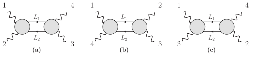
Figure 1: The (a) $s$-, (b) $t$- and (c) $u$-channel two-particle cuts of a one-loop four-point amplitude. The exposed lines are all on shell and the blobs represent tree-level amplitudes.

Traditionally, unitarity of the scattering matrix is implemented at the integrated level via dispersion relations (see e.g. Ref. AnalyticSMatrixBook ). However, for our purposes, it is much more convenient to use an integrand-level version of unitarity Unitarity . This is based on the concept of a generalized-unitarity cut that reduces an integrand to a sum of products of tree-level amplitudes. For example, for the $s$-channel cut displayed in Fig. 1(a),

$$i\mathcal{M}_{4}^{\text{1-loop}}\Big{\rvert}_{s\rm\hbox{-}cut}\!\!=\!\int\!\!\frac{d^{4-2\epsilon}L}{(2\pi)^{4-2\epsilon}}\frac{1}{L_{1}^{2}-m^{2}}\frac{1}{L_{2}^{2}-m^{2}}\sum_{\rm states}\!\mathcal{M}_{4}^{\rm tree}(1,2,L_{1},L_{2})\mathcal{M}_{4}^{\rm tree}(-L_{1},-L_{2},3,4)\Big{\rvert}_{s\rm\hbox{-}cut},$$ (9)

where $L_{1}=L$ and $L_{2}=-L-k_{1}-k_{2}$ represent the two cut legs, and $\mathcal{M}_{4}^{\rm tree}$ denote the tree-level amplitudes. The sum runs over all intermediate physical states that contribute for a given set of external states. The three generalized-unitarity cuts of the one-loop four-point amplitude are shown in Fig. 1. In this figure the exposed lines are all on shell and the blobs represent on-shell tree-level amplitudes.

To obtain the full one-loop amplitude we must combine the unitarity cuts. One possibility is to carry this out prior to integration by finding a single integrand with the correct unitarity cuts in all channels Bern:2004cz . Some non-trivial examples where this approach was implemented are high-loop computations in super-Yang-Mills and supergravity (see e.g. Refs. SuperHighLoopExamples ). On the other hand, in high-multiplicity QCD calculations (see e.g. Ref. BlackHat ) the cuts are usually combined after reducing to a basis of integrals. We apply the latter approach here. We do so by promoting each cut propagator to a Feynman propagator, and each cut to a Feynman integral. We then use FIRE6 Smirnov:2019qkx to reduce each Feynman integral to the scalar integrals appearing in Eq. (7). In each cut channel we only determine coefficients of basis integrals with cuts in that channel. By systematically evaluating each cut we determine all coefficients except for those of integrals without kinematic dependence, i.e. $I_{2}(0)$ and $I_{1}$. In the case of gauge theory, the corresponding coefficients are determined by imposing the known ultraviolet behavior of the amplitudes BernMorgan . Below, we describe an analogous procedure for the case of gravitational amplitudes.

Double copy

To efficiently obtain the unitarity cuts of the four-graviton amplitude, we use the double-copy construction Kawai:1985xq ; BCJ which expresses gravitational scattering amplitudes directly in terms of gauge-theory ones. Here we use the BCJ form of the double-copy relations BCJ ; BCJReview , which is more natural when organizing expressions in terms of diagrams.

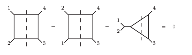
Figure 2: Example of a color or numerator relation for the one-loop four-point amplitudes. Here the diagram represent either color or kinematic numerators. We use these relations on the generalized-unitarity cuts, as indicated by the dashed lines. The relations are effectively tree-level ones except that the state and color sums on the cut legs are carried out.

To apply the BCJ double copy, we start by writing a four-point one-loop gauge-theory amplitude in the following form:

$$i\mathcal{A}_{4}^{\text{1-loop}}=g^{4}\sum_{i}\int\frac{d^{4-2\epsilon}L}{(2\pi)^{4-2\epsilon}}\frac{1}{S_{i}}\frac{n_{i}c_{i}}{D_{i}}\,.$$ (10)

The sum runs over all distinct four-point one-loop graphs with trivalent vertices. We denote the gauge-theory coupling constant by $g$. We label each graph by an integer $i$. The $S_{i}$ are the symmetry factors of the graphs. The color factor $c_{i}$ of each graph is obtained by dressing each vertex by a structure constant $\tilde{f}^{abc}$, since we take all particles to be in the adjoint representation. Our normalization of the structure constants follows that of Ref. BCJ . The denominator $D_{i}$ contains the propagators of each graph. Finally, we capture all non-trivial kinematic dependence by the numerator $n_{i}$.

The color factors obey color-algebra relations of the type

$$c_{i}-c_{j}-c_{k}=0\,,$$ (11)

where $i$, $j$ and $k$ are some graphs. These relations follow from the Jacobi identity obeyed by the structure constants $\tilde{f}^{abc}$. For a representation obeying color-kinematics duality, the numerators satisfy the same Jacobi relations, i.e.

$$\tilde{n}_{i}-\tilde{n}_{j}-\tilde{n}_{k}=0\,.$$ (12)

The tildes on the numerators signify that these numerators do not have to be the same as the ones appearing in Eq. (10), but as noted in Ref. BCJ these can be kinematic numerators from a different theory. Given such a representation we may obtain the corresponding gravitational amplitude simply by replacing the color factor with the corresponding kinematic numerator,

$$c_{i}\rightarrow\tilde{n}_{i}\,,$$ (13)

so that

$$i\mathcal{M}_{4}^{\text{1-loop}}=\left(\frac{\kappa}{2}\right)^{4}\sum_{i}\int\frac{d^{4-2\epsilon}L}{(2\pi)^{4-2\epsilon}}\frac{1}{S_{i}}\frac{n_{i}\tilde{n}_{i}}{D_{i}}\,,$$ (14)

where $\kappa$ is the gravitational coupling constant, which is given in terms of Newton’s constant by,

$$\kappa^{2}=32\pi G\,.$$ (15)

The matter content of the resulting gravitational theory is determined by the choice of the numerators $n_{i}$ and $\tilde{n}_{i}$. We use this to control the type of particle circulating in the loop.

While the BCJ double copy is usually formulated at the level of the full integrand, since we extract the final answer directly from the cuts it is more convenient to use it at the level of generalized-unitarity cuts. In Fig. 2 we depict an example of a color relation in terms of cut graphs. In this way we can ignore duality relations that contain diagrams without support on the given cut. For duality relations with support on the cut, the particles of each tree-level amplitude entering the cut remain on the same side of the cut for all three diagrams, as is the case in Fig. 2. Effectively this amounts to using the duality relations for the two tree-level amplitudes on each side of the cut (see e.g. Fig. 3). The tree-level relations are sufficient to ensure that for the cut diagram, the double-copy replacement formula (13) holds.

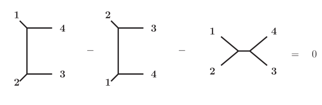
Figure 3: The tree-level four-point color or numerator Jacobi identity. This can be used to set the numerator of one of the diagrams to zero.

We also take advantage of a property of four-point tree-level amplitudes noted in the original BCJ paper BCJ , which states that we can effectively set one of the three numerators to zero. In this way the duality relation implies that the other two numerators must be equal (up to a possible sign). In order to achieve that, we absorb the propagator of the diagram whose numerator is set to zero into the numerators of the other two diagrams. Specifically, consider the four-point all-gluon tree-level amplitude,

$$i\mathcal{A}_{4}^{\text{tree}}=g^{2}\Bigl{(}\frac{n_{s}c_{s}}{s}+\frac{n_{t}c_{t}}{t}+\frac{n_{u}c_{u}}{u}\Bigr{)}\,.$$ (16)

Using the color Jacobi identity depicted in Fig. 3, $c_{s}=c_{t}-c_{u}$, we can eliminate $c_{s}$ in favor of the other two color factors, so that

$$i\mathcal{A}_{4}^{\text{tree}}=g^{2}\Bigl{(}\frac{n_{t}^{\prime}c_{t}}{t}+\frac{n_{u}^{\prime}c_{u}}{u}\Bigr{)}\,,$$ (17)

where

$$n_{t}^{\prime}=n_{t}+n_{s}\frac{t}{s}\,,\hskip 56.9055ptn_{u}^{\prime}=n_{u}-n_{s}\frac{u}{s}\,.$$ (18)

Demanding that the numerators $n_{t}^{\prime}$ and $n_{u}^{\prime}$ (and $n_{s}^{\prime}=0$) satisfy the duality relation of Fig. 3 then implies that

$$n_{t}^{\prime}=n_{u}^{\prime}\,.$$ (19)

The analysis is identical in the presence of matter.

II.2 Setup of the calculation

Our goal is to obtain the four-point one-loop amplitude with external gravitons and with minimally-coupled massive spinning particles up to spin 2 circulating in the loop. Following the generalized-unitarity method we first build the integrand-level generalized-unitarity cuts in Eq. (9). For the one-loop four-point amplitude there are three independent cuts, labeled by the Mandelstam invariant that can be build out of the external graviton momenta on the tree-level amplitudes, i.e. $s$-, $t$- and $u$-channel cuts. We consider all spins up to spin 2 for the massive particles and we denote their mass by $m$. While these masses can be different for each particle since only a single particle at a time circulates in the loop there is no need to put an index labeling the massive particle. We take the massive particles to be real.

We note that there is an ambiguity in the definition of the minimal coupling of a spin 2 particle to gravity. In this paper, we fix this ambiguity by demanding that we recover pure gravity in the appropriate massless limit. This choice also preserves tree-level unitarity treeLevelUnitarity and causality Bonifacio:2017nnt . We discuss this ambiguity and the choice we make in this paper in Appendix A.

For the amplitude in question there exist three independent helicity configurations. Specifically, we calculate

$$\mathcal{M}_{4}^{\text{1-loop}}(1^{+},2^{-},3^{-},4^{+})\,,\hskip 28.45274pt\mathcal{M}_{4}^{\text{1-loop}}(1^{+},2^{+},3^{-},4^{+})\,,\hskip 28.45274pt\mathcal{M}_{4}^{\text{1-loop}}(1^{+},2^{+},3^{+},4^{+})\,.$$ (20)

We refer to these configurations respectively as double-minus, single-minus and all-plus. All other amplitudes are related to these via relabelings and parity.

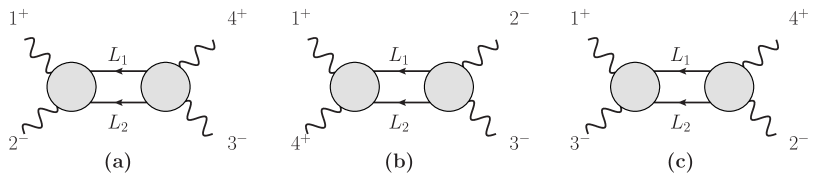
Figure 4: The (a) $s$-, (b) $t$- and (c) $u$-channel two-particle cuts of a one-loop four-point amplitude with two negative- and two positive-helicity external gluons or gravitons (double-minus configuration). The internal lines represent massive spinning particles. The exposed lines are all on shell and the blobs represent tree-level amplitudes.

We build the generalized-unitarity cuts from four-point tree-level gravity amplitudes. The double copy implies that these tree-level amplitudes can be directly obtained from the corresponding gauge-theory ones, which can be described by the three diagrams shown in Fig. 3. As we discussed in the previous section we can use the color Jacobi identity in the gauge-theory case to remove one diagram, at the expense of other diagrams obtaining numerators that are nonlocal in the external kinematic invariants. The net effect is that after multiplying and dividing by appropriate propagators every contribution to the cut can be assigned to cut box diagrams. Moreover, on the generalized cuts the four-point tree-level BCJ numerator relations set the remaining numerators equal to each other, as noted in Eq. (19).

For example, for the four-point gauge-theory amplitude the $s$-channel cut in Fig. 4(a) is of the form,

$$i\mathcal{A}_{4}\Big{\rvert}_{s\rm\hbox{-}cut}=g^{4}\int\frac{d^{4-2\epsilon}L}{(2\pi)^{4-2\epsilon}}\,n_{\text{g},s}\left(\frac{c_{1234}}{D_{1234}}+\frac{c_{1342}}{D_{1342}}\right)\bigg{\rvert}_{s\rm\hbox{-}cut}\,.$$ (21)

The box color factor (see Fig. 5) is given by

$$c_{abcd}=\tilde{f}^{e_{a}g_{1}g_{4}}\tilde{f}^{e_{b}g_{2}g_{1}}\tilde{f}^{e_{c}g_{3}g_{2}}\tilde{f}^{e_{d}g_{4}g_{3}}\,,$$ (22)

where $abcd$ takes in the values indicated in Eq. (21). As usual, repeated indices are summed. The denominators are given by products of the usual Feynman propagators,

$$D_{abcd}=\Big{(}L^{2}-m^{2}\Big{)}\Big{(}(L+k_{a})^{2}-m^{2}\Big{)}\Big{(}(L+k_{a}+k_{b})^{2}-m^{2}\Big{)}\Big{(}(L+k_{a}+k_{b}+k_{c})^{2}-m^{2}\Big{)}\,,$$ (23)

where the $k_{a}$ are external momenta. Finally, $n_{\text{g},s}$ is a gauge-theory kinematic factor common to both box diagrams.

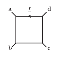
Figure 5: Generic box diagram whose color factor and denominator are given by Eqs. (22) and (23) respectively. The external momenta are taken incoming while the direction of the loop momentum is indicated by the arrow.

The gravitational cuts are similar. For example, the $s$-channel cut is of the form,

$$i\mathcal{M}_{4}\Big{\rvert}_{s\rm\hbox{-}cut}=\left(\frac{\kappa}{2}\right)^{4}\int\frac{d^{4-2\epsilon}L}{(2\pi)^{4-2\epsilon}}\,n_{\text{GR},s}\left(\frac{1}{D_{1234}}+\frac{1}{D_{1342}}\right)\bigg{\rvert}_{s\rm\hbox{-}cut}\,,$$ (24)

where $n_{\text{GR},s}$ is the single $s$-channel gravitational kinematic numerator. As we noted in Sect. II.1, the gravity amplitudes follow from replacing the color factor with a gauge-theory kinematic numerator. As we describe in more detail below, the particle content circulating in the loop is determined by the choice of the gauge-theory numerators.

As can be seen from Figs. 4(a) and 4(c), for the indicated helicity configuration, the $u$-channel cut is obtained by relabeling the momenta and spinors in the $s$-channel cut: $k_{2}\leftrightarrow k_{3}$ and $\langle 2|\leftrightarrow\langle 3|$. For the single-minus and all-plus configurations, all three cuts are given by appropriate relabelings of a single cut.

II.3 Supersymmetric decompositions

We are interested in the problem of minimally-coupled massive matter circulating in the loop. A convenient way to organize this calculation is by following the massless case where each particle can be described as a linear combination of supersymmetric multiplets circulating in the loop. Our organization is in direct correspondence to this supersymmetric decomposition SusyDecomposition ; Dunbar:1994bn ; Bern:1993tz . This allows us to recycle the results of the calculation of the lower-spin particles circulating in the loop into contributions for the higher-spin particles. It also has the advantage of grouping together terms that contain integrals of the same tensor rank. For the gauge-theory case such a decomposition has already been used to organize the contributions of massive spin $0$, $1/2$ and $1$ particles circulating in the loops Bern:1993tz ; BernMorgan . The double-copy construction will allow us to import this into minimally-coupled gravitational theories with up to spin-2 massive particles.

Gauge theory

We start by examining the corresponding amplitudes in gauge theory. For the case of one-loop four-point amplitudes with external gluons and massive matter circulating in the loop, Ref. Bern:1993tz showed that

$$\begin{split}\mathcal{A}_{4}^{S=0}&=\mathcal{A}_{4}^{\{0\}}\,,\\ \mathcal{A}_{4}^{S=1/2}&=-2\mathcal{A}_{4}^{\{0\}}+\mathcal{A}_{4}^{\{1/2\}}\,,\\ \mathcal{A}_{4}^{S=1}&=3\mathcal{A}_{4}^{\{0\}}-4\mathcal{A}_{4}^{\{1/2\}}+\mathcal{A}_{4}^{\{1\}}\,.\end{split}$$ (25)

where the notation $\mathcal{A}_{4}^{\{\it S\}}$ denotes the new piece we need to calculate at spin-$S$. In this way we express the amplitudes with a given spinning particle circulating in the loop in terms of the simpler-to-calculate new pieces. Inverting the above equations, we may think of the new pieces as amplitudes with multiplets circulating in the loop. These massive multiplets have the same degrees of freedom as the corresponding massless ones. Hence, in terms of on-shell supersymmetric representation theory they satisfy the BPS condition susyRepReviews . For recent calculations involving massive supersymmetric multiplets in gauge theory see Refs. n4symCoulombBranch ; Alday:2009zm .

Before turning to the corresponding gravitational decomposition it is useful to first look at the massless limit. For the gauge theory case we have that as $m\rightarrow 0$,

$$\begin{split}\mathcal{A}_{4}^{S=0}&\rightarrow\mathcal{A}_{4}^{S=0,\,\textit{m}=0}\,,\\ \mathcal{A}_{4}^{S=1/2}&\rightarrow\mathcal{A}_{4}^{S=1/2,\,\textit{m}=0}\,,\\ \mathcal{A}_{4}^{S=1}&\rightarrow\mathcal{A}_{4}^{S=1,\,\textit{m}=0}+\mathcal{A}_{4}^{S=0,\,\textit{m}=0}\,,\end{split}$$ (26)

where we see that the $S=1$ case is nontrivial, which follows from the mismatch in the number of degrees of freedom in a massive and massless vector boson.

Background field gauge

A nice way to understand the above supersymmetric decomposition is in terms of background field gauge UnitarityReview1 . While we do not use background field gauge to compute the amplitudes, it does offer useful insight into the structure of the amplitude. For the different particles circulating in the loop we can write the effective action as

$$\Gamma_{S=0}[A] =\ln\det{}_{[0]}^{-1/2}\bigl{(}D^{2}+m^{2}\bigr{)}\,,$$

$$\Gamma_{S=1/2}[A] =\ln\det{}_{[1/2]}^{1/4}\bigl{(}D^{2}\,\mathbb{I}+m^{2}\,\mathbb{I}-g\frac{1}{2}\sigma^{\mu\nu}F_{\mu\nu})\,,$$ (27)

$$\Gamma_{S=1}[A] =\ln\det{}_{[1]}^{-1/2}\bigl{(}D^{2}\mathbb{I}+m^{2}\mathbb{I}-g\Sigma^{\mu\nu}F_{\mu\nu}\bigl{)}+\ln\det{}_{[0]}\bigl{(}D^{2}+m^{2}\bigr{)}+\ln\det{}_{[0]}^{-1/2}\bigl{(}D^{2}+m^{2}\bigr{)}\,,$$

where $\mathbb{I}$ is the identity matrix, $\sigma_{\mu\nu}/2$ is the spin-$1/2$ Lorentz generator and $\Sigma_{\mu\nu}$ is the spin-1 Lorentz generator. Ignoring the $F_{\mu\nu}$ terms and focusing on the $(D^{2}+m^{2})$ term, each state corresponds to a power to which the determinant is raised: $-1/2$ for a bosonic state and $+1/2$ for a fermionic state. For a massive real scalar there is precisely one bosonic state corresponding the $-1/2$ power to which the first determinant is raised. For the $S=1/2$ fermion the determinant is raised to the $1/4$ power to account for the $4\times 4$ Dirac determinant, effectively leaving a single power that corresponds to the two states of a Majorana fermion. Similarly, for the $S=1$ vector, the determinant is over a $4\times 4$ Lorentz generator space so the exponent of $-1/2$ in the first term in $\Gamma_{S=1}[A]$ corresponds to 4 bosonic states. This is then reduced to two states by the ghost determinant corresponding to the second term and increased by one state from the scalar longitudinal degree of freedom required by a massive vector boson corresponding to the third term. This extra degree of freedom is incorporated into Eq. (25) as well. To make the supersymmetric cancellations more manifest we rewrite the Dirac determinant as a product of determinants so that the similarity to the bosonic case is clear,

$$\det{}_{[1/2]}^{1/2}({\raise 0.91666pt\hbox to8.55695pt{\hss/\hss}\hbox to0.0pt{\hss$D$}}+im)\det{}_{[1/2]}^{1/2}({\raise 0.91666pt\hbox to8.55695pt{\hss/\hss}\hbox to0.0pt{\hss$D$}}-im) =\det{}_{[1/2]}^{1/4}({\raise 0.91666pt\hbox to8.55695pt{\hss/\hss}\hbox to0.0pt{\hss$D$}}^{2}+m^{2})$$

$$=\det{}_{[1/2]}^{1/4}(D^{2}+m^{2}-g\frac{1}{2}\sigma^{\mu\nu}F_{\mu\nu})\,,$$ (28)

where ${\raise 0.91666pt\hbox to8.55695pt{\hss/\hss}\hbox to0.0pt{\hss$D$}}^{2}=\frac{1}{2}\{{\raise 0.91666pt\hbox to8.55695pt{\hss/\hss}\hbox to0.0pt{\hss$D$}},{\raise 0.91666pt\hbox to8.55695pt{\hss/\hss}\hbox to0.0pt{\hss$D$}}\}+\frac{1}{2}[{\raise 0.91666pt\hbox to8.55695pt{\hss/\hss}\hbox to0.0pt{\hss$D$}},{\raise 0.91666pt\hbox to8.55695pt{\hss/\hss}\hbox to0.0pt{\hss$D$}}]$. This corresponds to using the second order formalism for fermions described in Ref. SecondOrderFermions . The fact that the mass enters into Eq. (27) in such a simple manner can also be understood in terms of a Kaluza-Klein reduction of the massless case from five dimensions, truncated to keeping only the lowest massive state in the loop.

The effective-action determinants (27) can be straightforwardly applied to show that the supersymmetric decomposition organizes contributions in terms of power counting of the resulting diagrams. The terms with leading power of loop momenta come from the $D^{2}$ terms in Eq. (27), because $F_{\mu\nu}$ contains only the external gluon momenta. If we set the $F_{\mu\nu}$ terms to zero then in all supersymmetric combinations the balance between the bosons and fermions implies the leading powers of loop momentum cancel. Subleading terms in supersymmetric combinations come from using one or more factors of $F_{\mu\nu}$ when generating a graph; each $F_{\mu\nu}$ reduces the maximum power of momentum by one. Terms with a lone $F_{\mu\nu}$ vanish, thanks to ${\rm Tr}(\sigma^{\mu\nu})={\rm Tr}(\Sigma^{\mu\nu})=0$. This reduces the leading power in an $m$-point one-particle-irreducible diagram from $\ell^{m}$ down to $\ell^{m-2}$. For $\mathcal{A}_{m}^{\{1\}}$, a comparison of the traces of products of two and three $\sigma^{\mu\nu}$ and $\Sigma_{\mu\nu}$ shows that further cancellations reduce the leading behavior all the way down to $\ell^{m-4}$. In gauges other than Feynman background field gauge, these cancellations would be more more obscure.

Gravity

Now consider the gravitational case. In the $m\rightarrow 0$ limit we again have a mismatch in the number of degrees of freedom for $S\geq 1$ between the massive and massless cases,

$$\begin{split}\mathcal{M}_{4}^{S=0}&\rightarrow\mathcal{M}_{4}^{S=0,\,\textit{m}=0}\,,\\ \mathcal{M}_{4}^{S=1/2}&\rightarrow\mathcal{M}_{4}^{S=1/2,\,\textit{m}=0}\,,\\ \mathcal{M}_{4}^{S=1}&\rightarrow\mathcal{M}_{4}^{S=1,\,\textit{m}=0}+\mathcal{M}_{4}^{S=0,\,\textit{m}=0}\,,\\ \mathcal{M}_{4}^{S=3/2}&\rightarrow\mathcal{M}_{4}^{S=3/2,\,\textit{m}=0}+\mathcal{M}_{4}^{S=1/2,\,\textit{m}=0}\,,\\ \mathcal{M}_{4}^{S=2}&\rightarrow\mathcal{M}_{4}^{S=2,\,\textit{m}=0}+\mathcal{M}_{4}^{S=1,\,\textit{m}=0}+\mathcal{M}_{4}^{S=0,\,\textit{m}=0}\,.\end{split}$$ (29)

In the massless case with spinning particles circulating in the loop we can again decompose the amplitudes in terms of ones with supermultiplets circulating in the loop Dunbar:1994bn ,

$$\begin{split}\mathcal{M}_{4}^{S=0,\,\textit{m}=0}&=\mathcal{M}_{4}^{\{0\},\,\textit{m}=0}\,,\\ \mathcal{M}_{4}^{S=1/2,\,\textit{m}=0}&=-2\mathcal{M}_{4}^{\{0\},\,\textit{m}=0}+\mathcal{M}_{4}^{\{1/2\},\,\textit{m}=0}\,,\\ \mathcal{M}_{4}^{S=1,\,\textit{m}=0}&=2\mathcal{M}_{4}^{\{0\},\,\textit{m}=0}-4\mathcal{M}_{4}^{\{1/2\},\,\textit{m}=0}+\mathcal{M}_{4}^{\{1\},\,\textit{m}=0}\,,\\ \mathcal{M}_{4}^{S=3/2,\,\textit{m}=0}&=-2\mathcal{M}_{4}^{\{0\},\,\textit{m}=0}+9\mathcal{M}_{4}^{\{1/2\},\,\textit{m}=0}-6\mathcal{M}_{4}^{\{1\},\,\textit{m}=0}+\mathcal{M}_{4}^{\{3/2\},\,\textit{m}=0}\,,\\ \mathcal{M}_{4}^{S=2,\,m=0}&=2\mathcal{M}_{4}^{\{0\},\,\textit{m}=0}-16\mathcal{M}_{4}^{\{1/2\},\,\textit{m}=0}+20\mathcal{M}_{4}^{\{1\},\,\textit{m}=0}-8\mathcal{M}_{4}^{\{3/2\},\,\textit{m}=0}\\ &\hskip 14.22636pt+\mathcal{M}_{4}^{\{2\},\,\textit{m}=0}\,.\end{split}$$ (30)

The $\{S\}$ pieces in each case are in direct correspondence to the supermultiplets circulating in the loop, as defined in Ref. Dunbar:1994bn . For example,

$$\mathcal{M}_{4}^{\{1/2\},\,\textit{m}=0}=\mathcal{M}_{4}^{\mathcal{N}=1,\,\textit{m}=0},$$ (31)

where $\mathcal{N}=1$ denotes the chiral multiplet consisting of a Weyl fermion and two real scalars.

Using the relation between the massive and massless amplitudes in Eq. (29) and the massless supersymmtric decomposition in Eq. (30), we can organize our computation in a similar way as for gauge theory in Eq. (25). Specifically, we have

$$\begin{split}\mathcal{M}_{4}^{S=0}&=\mathcal{M}_{4}^{\{0\}}\,,\\ \mathcal{M}_{4}^{S=1/2}&=-2\mathcal{M}_{4}^{\{0\}}+\mathcal{M}_{4}^{\{1/2\}}\,,\\ \mathcal{M}_{4}^{S=1}&=3\mathcal{M}_{4}^{\{0\}}-4\mathcal{M}_{4}^{\{1/2\}}+\mathcal{M}_{4}^{\{1\}}\,,\\ \mathcal{M}_{4}^{S=3/2}&=-4\mathcal{M}_{4}^{\{0\}}+10\mathcal{M}_{4}^{\{1/2\}}-6\mathcal{M}_{4}^{\{1\}}+\mathcal{M}_{4}^{\{3/2\}}\,,\\ \mathcal{M}_{4}^{S=2}&=5\mathcal{M}_{4}^{\{0\}}-20\mathcal{M}_{4}^{\{1/2\}}+21\mathcal{M}_{4}^{\{1\}}-8\mathcal{M}_{4}^{\{3/2\}}+\mathcal{M}_{4}^{\{2\}}\,.\end{split}$$ (32)

The massive multiplets circulating in the loop are ‘short’, i.e. they have the same degrees of freedom as the corresponding massless ones. Hence, they obey the BPS condition susyRepReviews . While we have not tried directly embedding these amplitudes into supergravity theories, it is an interesting question to do so. Here we use the relation to supermultiplets for a more modest aim of reorganizing the contributions, so that as the spin increases the new pieces become simpler. Examples of supergravity calculations involving massive multiplets are given in Ref. massiveSugra .

We note that in general, care is required when using dimensional regularization in conjunction with helicity methods and supersymmetric decompositions. To allow for different choices of regularization scheme, we would need to correct the last line of Eq. (25) to be Bern:1993tz

$$\mathcal{A}_{4}^{S=1}=(3-2\delta_{R}\epsilon)\mathcal{A}_{4}^{\{0\}}-4\mathcal{A}_{4}^{\{1/2\}}+\mathcal{A}_{4}^{\{1\}},$$ (33)

where $\delta_{R}=0$ in the FDH scheme Bern:1991aq and $\delta_{R}=1$ in either conventional dimensional regularization Collins or the ’t Hooft-Veltman scheme tHooft:1972tcz . One may then propagate this correction to the gravitational amplitudes through the double copy. While the correction is of $\mathcal{O}(\epsilon)$, it can interfere with infrared or ultraviolet singularities to give nontrivial contributions. However, for the massive amplitudes that we are computing here, the distinction between different schemes is not important because the four-graviton amplitudes with massive matter in the loop are both ultraviolet and infrared finite (see Sects. II.6 and II.8).

We also note that the coefficient of the scalar ($\mathcal{M}_{4}^{\{0\}}$) counts the degrees of freedom of the particle in question, modulo a minus sign for the fermions. Recall that all particles are taken to be real. Also, given the general setup of our amplitudes (Eqs. (21) and (24)), we get a similar decomposition for the corresponding numerators $n_{\text{g},\alpha}$ and $n_{\text{GR},\alpha}$.

Finally, the supersymmetric decomposition is simplified in the case of the single-minus and all-plus configurations. In these cases, supersymmetric Ward identities SWI show that only the $\mathcal{M}_{4}^{\{0\}}$ piece gives a nonzero contribution for each spin particle in the loop. Using this observation, Eq. (32) becomes

$$\begin{split}\mathcal{M}_{4}^{S=0}(1^{\pm},2^{+},3^{+},4^{+})&=\mathcal{M}_{4}^{\{0\}}(1^{\pm},2^{+},3^{+},4^{+})\,,\\ \mathcal{M}_{4}^{S=1/2}(1^{\pm},2^{+},3^{+},4^{+})&=-2\mathcal{M}_{4}^{\{0\}}(1^{\pm},2^{+},3^{+},4^{+})\,,\\ \mathcal{M}_{4}^{S=1}(1^{\pm},2^{+},3^{+},4^{+})&=3\mathcal{M}_{4}^{\{0\}}(1^{\pm},2^{+},3^{+},4^{+})\,,\\ \mathcal{M}_{4}^{S=3/2}(1^{\pm},2^{+},3^{+},4^{+})&=-4\mathcal{M}_{4}^{\{0\}}(1^{\pm},2^{+},3^{+},4^{+})\,,\\ \mathcal{M}_{4}^{S=2}(1^{\pm},2^{+},3^{+},4^{+})&=5\mathcal{M}_{4}^{\{0\}}(1^{\pm},2^{+},3^{+},4^{+})\,.\end{split}$$ (34)

Therefore for these two helicity configurations, it is sufficient to calculate the $S=0$ amplitude where only a scalar circulates in the loop.

II.4 Kinematic numerators through the double copy

Following the double-copy construction we can directly obtain the gravitational unitarity-cut numerators from gauge-theory ones. We may express the double copy in terms of spinning particles or new pieces (Eq. (32)) circulating in the loop. In the latter case, we find an especially compact representation for the numerators.

Taking the product of gauge-theory kinematic numerators we decompose them into cut numerators of the gravitational case. In terms of spin we have

$$\begin{split}n_{\text{g},\alpha}^{\tilde{S}}n_{\text{g},\alpha}^{S=0}&=n_{\text{GR},\alpha}^{\tilde{S}}\,,\qquad\hbox{for $\tilde{S}=0,1/2,1$}\,,\\ n_{\text{g},\alpha}^{S=1/2}n_{\text{g},\alpha}^{S=1/2}&=n_{\text{GR},\alpha}^{S=1}+n_{\text{GR},\alpha}^{S=0}\,,\\ n_{\text{g},\alpha}^{S=1}n_{\text{g},\alpha}^{S=1/2}&=n_{\text{GR},\alpha}^{S=3/2}+n_{\text{GR},\alpha}^{S=1/2}\,,\\ n_{\text{g},\alpha}^{S=1}n_{\text{g},\alpha}^{S=1}&=n_{\text{GR},\alpha}^{S=2}+n_{\text{GR},\alpha}^{S=1}+n_{\text{GR},\alpha}^{S=0}\,,\end{split}$$ (35)

where $\alpha$ denotes the cut under consideration. These are in direct correspondence to the Clebsch-Gordan decomposition. In terms of the new pieces in Eq. (32),

$$\begin{split}n_{\text{g},\alpha}^{\{\it S\}}n_{\text{g},\alpha}^{\{0\}}&=n_{\text{GR},\alpha}^{\{\it S\}}\,,\qquad\hbox{for $S=0,1/2,1$ },\\ n_{\text{g},\alpha}^{\{1/2\}}n_{\text{g},\alpha}^{\{1/2\}}&=n_{\text{GR},\alpha}^{\{1\}}\,,\\ n_{\text{g},\alpha}^{\{1\}}n_{\text{g},\alpha}^{\{1/2\}}&=n_{\text{GR},\alpha}^{\{3/2\}}\,,\\ n_{\text{g},\alpha}^{\{1\}}n_{\text{g},\alpha}^{\{1\}}&=n_{\text{GR},\alpha}^{\{2\}}\,.\end{split}$$ (36)

Observe that the gauge-theory numerator $n_{\text{g},\alpha}^{S=0}$ along with either $n_{\text{g},\alpha}^{S=1/2}$ or $n_{\text{g},\alpha}^{S=1}$ are sufficient to construct all the gravitational numerators up to spin 2. We explicitly verified that both constructions yield the same result. Refs. Bern:1993tz ; BernMorgan calculated the corresponding amplitudes $\mathcal{A}_{4}^{S=0}$, $\mathcal{A}_{4}^{S=1/2}$ and $\mathcal{A}_{4}^{S=1}$, from which we may extract the desired kinematic numerators. As a consistency check, we match $\mathcal{A}_{4}^{\{1\}}$, which was calculated in Ref. Alday:2009zm .

From the above construction we find a remarkably simple form for the kinematic numerators. For the double-minus gauge-theory numerators we have,

$$n_{\text{g},\alpha}^{\{\it S\}}=\big{(}[14]\langle 23\rangle\big{)}^{2}(\psi_{\alpha})^{2-2S}\,,$$ (37)

while for the corresponding gravity numerators we have,

$$n_{\text{GR},\alpha}^{\{\it S\}}=\big{(}[14]\langle 23\rangle\big{)}^{4}(\psi_{\alpha})^{4-2S}\,,$$ (38)

where

$$\psi_{s}\equiv\frac{\langle 2|\ell|1]\langle 3|\ell|4]}{s[14]\langle 23\rangle}\,,\hskip 56.9055pt\psi_{t}\equiv\frac{(m^{2}+\mu^{2})}{t}\,,\hskip 56.9055pt\psi_{u}\equiv\frac{\langle 3|\ell|1]\langle 2|\ell|4]}{u[14]\langle 32\rangle}\,.$$ (39)

For the single-minus and all-plus configurations it is sufficient to calculate the numerators for a scalar circulating in the loop. For the single-minus configuration for gauge theory and gravity we find

$$n_{\text{g},s}^{S=0}=\frac{(m^{2}+\mu^{2})}{s}\frac{[12]}{\langle 12\rangle}\langle 3|\ell|4]^{2},\hskip 42.67912ptn_{\text{GR},s}^{S=0}=\frac{(m^{2}+\mu^{2})^{2}}{s^{2}}\frac{[12]^{2}}{\langle 12\rangle^{2}}\langle 3|\ell|4]^{4},$$ (40)

while for the all-plus configuration we have

$$n_{\text{g},s}^{S=0}=(m^{2}+\mu^{2})^{2}\frac{[12][34]}{\langle 12\rangle\langle 34\rangle}\,,\hskip 42.67912ptn_{\text{GR},s}^{S=0}=(m^{2}+\mu^{2})^{4}\Bigg{(}\frac{[12][34]}{\langle 12\rangle\langle 34\rangle}\Bigg{)}^{2}\,.$$ (41)

For these two configurations, we obtain the numerators for the $t$- and $u$-channel cuts by appropriate relabelings.

Following the conventions of Ref. BernMorgan , we break the $(4-2\epsilon)$-dimensional loop momentum $L$ into a four-dimensional part $\ell$ and a $(-2\epsilon)$-dimensional part $\mu$. We write $L=(\ell,\mu)$. Using this notation we have for example

$$\ell^{2}=m^{2}+\mu^{2}\,,$$ (42)

when the cut condition $L^{2}=m^{2}$ is satisfied. We take $\epsilon<0$ so that we can break the loop momentum in this fashion. Further, whenever a four-dimensional vector $v\equiv(v,0)$ is contracted with the $(4-2\epsilon)$-dimensional loop momentum, the $(-2\epsilon)$-dimensional part is projected out,

$$v\cdot L=v\cdot\ell\,.$$ (43)

Ref. Arkani-Hamed:2017jhn (Eqs. (5.20) and (5.36)) calculated Compton amplitudes for a massive particle in four dimensions of up to spin 1 in gauge theory and up to spin 2 in gravity. We find similar spin dependence in our double-minus numerators as for these Compton amplitudes.

II.5 Integral reduction and cut merging

In this subsection we use standard integration-by-parts (IBP) methods to reduce the generalized-unitarity cuts we calculated in the previous section in terms of a basis of master integrals. This allows us to fix all integral coefficients in Eq. (7) other than those of the tadpole and the bubble on external leg. We discuss these remaining pieces in Sect. II.6. We show details for the double-minus configuration with a scalar in the loop; the remaining helicity configurations and particle-in-the-loop contributions are similar. In order to keep the expressions concise, we do not include the helicity labels.

The general strategy for constructing the full amplitudes is to evaluate the cuts one by one in terms of the master integrals appearing in Eq. (7). If a given integral has a generalized cut in the channel being evaluated then that channel fully determines its coefficient. By stepping through the three channels in Fig. 1 we obtain the coefficients of all master integrals except $I_{2}(0)$ and $I_{1}$. The box integrals each have cuts in two channels so consistency requires that they give the same coefficient.

We start with the $s$-channel cut of the $S=0$ double-minus helicity configuration defined in Eq. (20). The discussion for the $u$-channel cut follows in the same way, since it is given by a relabeling of the $s$-channel one. We have

$$i\mathcal{M}_{4}^{S=0}\bigg{\rvert}_{s\text{-cut}}=\left(\frac{\kappa}{2}\right)^{4}(\langle 23\rangle[14])^{4}\int\frac{d^{4-2\epsilon}L}{(2\pi)^{4-2\epsilon}}\left(\frac{\langle 2|\ell|1]\langle 3|\ell|4]}{s[14]\langle 23\rangle}\right)^{4}\left(\frac{1}{D_{1234}}+\frac{1}{D_{1342}}\right)\bigg{\rvert}_{s\text{-cut}}.$$ (44)

We define

$$v_{1}^{\mu}=\langle 2|\gamma^{\mu}|1]\,,\,\hskip 56.9055ptv_{2}^{\mu}=\langle 3|\gamma^{\mu}|4]\,,$$ (45)

which live in the four-dimensional subspace so that the $v_{i}$ effectively project out the $(4-2\epsilon)$-dimensional components. This implies that $v_{i}\cdot\ell=v_{i}\cdot L$, as follows from the prescription BernMorgan that $\epsilon<0$ . Next, we lift the cut condition and regard our expression as part of the full integrand that we would have obtained by Feynman rules,

$$i\mathcal{M}_{4}^{S=0,\,s\text{-channel}}=\left(\frac{\kappa}{2}\right)^{4}(\langle 23\rangle[14])^{4}\int\frac{d^{4-2\epsilon}L}{(2\pi)^{4-2\epsilon}}\left(\frac{\langle 2|L|1]\langle 3|L|4]}{s[14]\langle 23\rangle}\right)^{4}\left(\frac{1}{D_{1234}}+\frac{1}{D_{1342}}\right),$$ (46)

keeping in mind that it is only valid for contributions that have an $s$-channel cut. We apply IBP identities IBP in $4-2\epsilon$ dimensions to reduce the above integrals to the master integrals in Eq. (7), using the software FIRE6 Smirnov:2019qkx . Upon reducing to master integrals we remove the ones that have no $s$-channel cut.

Next, we turn to the $t$-channel cut. We have

$$i\mathcal{M}_{4}^{S=0}\bigg{\rvert}_{t\text{-cut}}=\left(\frac{\kappa}{2}\right)^{4}(\langle 23\rangle[14])^{4}\int\frac{d^{4}\ell}{(2\pi)^{4}}\frac{d^{-2\epsilon}\mu}{(2\pi)^{-2\epsilon}}\left(\frac{(m^{2}+\mu^{2})}{t}\right)^{4}\left(\frac{1}{D_{1234}}+\frac{1}{D_{1423}}\right)\bigg{\rvert}_{t\text{-cut}},\quad$$ (47)

where we subdivide the integration into four- and $(-2\epsilon)$-dimensional parts

$$\int\frac{d^{4-2\epsilon}L}{(2\pi)^{4-2\epsilon}}=\int\frac{d^{4}\ell}{(2\pi)^{4}}\frac{d^{-2\epsilon}\mu}{(2\pi)^{-2\epsilon}}\,.$$ (48)

As for the $s$ channel, we lift the cut conditions and regard our expression as part of the full integrand,

$$i\mathcal{M}_{4}^{S=0,\,t\text{-channel}}=\left(\frac{\kappa}{2}\right)^{4}(\langle 23\rangle[14])^{4}\int\frac{d^{4}\ell}{(2\pi)^{4}}\frac{d^{-2\epsilon}\mu}{(2\pi)^{-2\epsilon}}\left(\frac{(m^{2}+\mu^{2})}{t}\right)^{4}\left(\frac{1}{D_{1234}}+\frac{1}{D_{1423}}\right).$$ (49)

As we discuss in Appendix G.2, the integrals with the $(-2\epsilon)$-dimensional components of loop-momentum $\mu$ in the numerators can be expressed directly in terms of the master integrals defined in Eq. (8). After reducing our expression we eliminate master integrals that vanish on the $t$-channel cut.

As noted above, an important consistency condition arises from the fact that the box integrals have cuts in two channels, so we can determine their coefficients from either channel. We explicitly verified that the coefficients we obtain for the box integrals from looking at the different channels are the same. In this way we are able to extract all coefficients of Eq. (7) other than $a_{0}$ and $b_{0}$, since the corresponding integrals have no cuts in any channel; we obtain these remaining two integral coefficients in Sect. II.6.

II.6 Ultraviolet behavior and rational pieces

Analyzing the different generalized-unitarity cuts we obtain all the coefficients in Eq. (7) other than $a_{0}$ and $b_{0}$. Tadpoles and bubbles on external legs (see Fig. 6) vanish on any cut, therefore their coefficients are not accessible through generalized unitarity. In this subsection we use the known UV properties of the amplitude to obtain these coefficients. Similarly to Sect. II.5, we discuss the double-minus configuration as a specific example. The other configurations follow in the same manner.

First, we observe that simply neglecting these two integrals leads to an inconsistent answer. Expanding to leading order in $\epsilon$ we get

$$\mathcal{M}_{4}^{S=0}\bigg{\rvert}_{a_{0}\rightarrow 0,\,b_{0}\rightarrow 0}=(\langle 23\rangle[14])^{4}\frac{m^{2}\tilde{Q}(s,t,m)}{\epsilon}+\mathcal{O}(\epsilon^{0})\,,$$ (50)

where $\tilde{Q}(s,t,m)$ is some rational function. We note that we expect no UV divergence to appear in the four-graviton amplitude since the only counterterm that we could write to absorb it is the Gauss-Bonnet term, which is evanescent in four dimensions tHooft:1974toh . Also, the UV divergence not coming out local hints that we neglected to include some integrals.

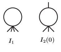
Figure 6: The tadpole and bubble-on-external-leg integrals.

We use the vanishing of the UV divergence to obtain the remaining coefficients $a_{0}$ and $b_{0}$. Note that since $a_{0}$ and $b_{0}$ are rational functions of $\epsilon$, it seems that we do not have enough information to fully fix them. We surpass this difficulty by realizing that our problem admits a second integral basis where the integral coefficients do not depend on $\epsilon$ and $m$. This basis is overcomplete in that it contains ($4-2\epsilon$)- and higher-dimensional integrals, while the one introduced in Eq. (7) only includes ($4-2\epsilon$)-dimensional integrals. We discuss this basis in detail and provide an algorithmic way of switching between the two bases in Appendix G.2.

We start by bringing the quantity we get from cut merging to the basis containing higher-dimensional integrals. In doing so, we remove any integrals that vanish on all cuts. We refer to this piece expressed in this basis as the ‘on-shell-constructable’ piece. Then, we need to figure out which integrals without unitarity cuts we need to include in our expression, since in principle one could add infinitely many higher-dimensional integrals.

We consider the pieces that would arise in a Feynman-rules calculation. For the amplitude at hand we would find integrals up to quartically divergent. After we IBP reduce them and express them in the basis that contains the higher-dimensional integrals, we would in principle find all scalar integrals up to quartically divergent appearing. Hence we need to consider:

$$I_{1},\qquad I_{2}(k^{2})\,,\qquad I_{1}^{6-2\epsilon}\,,\qquad I_{2}^{6-2\epsilon}(k^{2})\,,\qquad I_{2}^{8-2\epsilon}(k^{2})\,,$$ (51)

where we imagine the limiting case $k^{2}\rightarrow 0$. For our definition of higher-dimensional integrals see Eq. (279). These are all the integrals that have no unitarity cuts and are up to quartically divergent. The reason why we consider the above limiting case is because the coefficients of these integrals might have a $1/k^{2}$ pole.

Then, the unknown piece in our amplitude up to normalization takes the form

$$\lim_{k^{2}\rightarrow 0}\Big{(}\beta_{1}I_{1}+\beta_{2}I_{2}(k^{2})+\beta_{3}I_{1}^{6-2\epsilon}+\beta_{4}I_{2}^{6-2\epsilon}(k^{2})+\beta_{5}I_{2}^{8-2\epsilon}(k^{2})\Big{)}=\gamma_{1}I_{1}+\gamma_{2}I_{2}(0)+\gamma_{3}I_{1}^{6-2\epsilon}\,,$$ (52)

where we use

$$I_{2}^{6-2\epsilon}(k^{2})=I_{1}+\frac{k^{2}}{6}I_{2}(0)+\mathcal{O}(k^{4})\,,\quad\quad I_{2}^{8-2\epsilon}(k^{2})=I_{1}^{6-2\epsilon}+\frac{k^{2}}{6}I_{1}+\mathcal{O}(k^{4})\,,$$ (53)

following Appendix B of Ref. BernMorgan . The unknown coefficients $\gamma_{i}$ are rational functions of the kinematics that do not contain $\epsilon$ or $m$ dependence. In writing this expression we assume that the coefficients of the integrals are at worse divergent as $1/k^{2}$ and that the expression is finite in the $k^{2}\rightarrow 0$ limit when a massive particle is circulating in the loop.

Upon these considerations, our amplitude takes the form

$$\mathcal{M}_{4}^{S=0}=\mathcal{M}_{4}^{S=0}\bigg{\rvert}_{\text{on-shell-constr.}}+\frac{1}{(4\pi)^{2-\epsilon}}\left(\frac{\kappa}{2}\right)^{2}\mathcal{M}^{\text{tree}}_{4}\big{(}\gamma_{1}I_{1}+\gamma_{2}I_{2}(0)+\gamma_{3}I_{1}^{6-2\epsilon}\big{)}\,,$$ (54)

where the $\gamma_{i}$ are coefficients are determined from the requirement that ultraviolet divergences cancel, the integrals $I_{1}$ and $I_{2}$ are given in Eqs. (280) and (282), and

$$\mathcal{M}^{\text{tree}}_{4}\equiv\mathcal{M}^{\text{tree}}_{4}(1^{+},2^{-},3^{-},4^{+})=\left(\frac{\kappa}{2}\right)^{2}\frac{(\langle 23\rangle[14])^{4}}{stu}\,.$$ (55)

The Mandelstam variables are defined below Eq. (8). Note that the little-group scaling for the unknown terms is fixed to be $(\langle 23\rangle[14])^{4}$. Since the $\gamma_{i}$ are rational functions of the kinematics, we are free to multiply and divide by $(stu)$ to introduce $\mathcal{M}^{\text{tree}}_{4}$.

Next, demanding that the amplitude has no UV divergence and that all three $\gamma_{i}$ are independent of the mass $m$ uniquely fixes $\gamma_{1}$ and $\gamma_{3}$ to nonzero values while setting $\gamma_{2}=0$. The results for the amplitudes collected in Appendix F the values of the $\gamma_{i}$ are all chosen to make the amplitudes UV finite.

As a simple consistency check, we repeat this analysis adding integrals that have no unitarity cuts and are divergent worse than quartically (namely ($8-2\epsilon$)- and higher-dimensional tadpoles). We verify that the answer is the same, i.e. the coefficients of these new integrals are set to zero.

We now briefly comment on the $m\rightarrow 0$ limit. In this limit, both $I_{1}$ and $I_{2}(0)$ vanish, and the amplitude has no UV divergence, as can be seen from Eq. (50). Hence our amplitude has the correct UV behavior in this limit as well. Moreover, all integrals that have no unitarity cuts become scaleless and hence zero in dimensional regularization. Therefore, there are no unfixed coefficients and our construction based on the unitarity cuts captures the full amplitude.

Finally, we want to clarify why we chose the overcomplete basis with higher-dimensional integrals. The coefficients $a_{0}$ and $b_{0}$ are in principle arbitrary rational functions of $\epsilon$ and $m$, and of the kinematic variables $s$ and $t$. The existence of a basis where the integral coefficients do not contain $\epsilon$ or $m$ significantly restricts the functional dependence of $a_{0}$ and $b_{0}$ on $\epsilon$ and $m$. The existence of such a basis is a nontrivial fact that may be understood via analyzing the calculation in a covariant gauge, as we explain in Appendix G.2. In this way the two integral bases are not completely equivalent, since the latter one is exploiting more of the specific properties of the problem at hand.

II.7 Further ultraviolet properties

Quadratic and quartic divergence

Next, we want to analyze the quadratic and quartic divergence of our amplitude. In dimensional regularization, the signature of these divergences are poles around $\epsilon=1$ and $\epsilon=2$ in the final answer. Since we compute our amplitude to all order in $\epsilon$ we may probe these poles. We tackle this question in the basis that contains only ($4-2\epsilon$)-dimensional integrals. In the basis that includes higher-dimensional integrals, many of the integrals are quadratically or quartically divergent, which obscures the analysis. We discuss the double-minus configuration for a spin-0 particle in the loop; the other cases are similar. As we demonstrate, our amplitude has no quadratic or quartic divergences.

We start with the quadratic divergence. In the chosen basis the only quadratically divergent integral is the tadpole. However, the coefficient of the tadpole is linear in $(\epsilon-1)$, hence there is no contribution to the quadratic divergence from it. It then suffices to expand all coefficients around $\epsilon=1$ and only keep the divergent piece. We get

$$\mathcal{M}_{4}^{S=0} =-\frac{1}{(4\pi)^{2-\epsilon}}\left(\frac{\kappa\hbox{}}{2}\right)^{2}\mathcal{M}^{\text{tree}}_{4}\frac{su}{(\epsilon-1)t^{6}}(3s^{2}u^{2}+10m^{2}stu+6m^{4}t^{2})\Big{(}\iota_{2}(s)+\iota_{2}(u)\Big{)}$$

$$\hskip 85.35826pt\hbox{}+\mathcal{O}\Big{(}(\epsilon-1)^{0}\Big{)}\,,$$ (56)

where we introduced

$$\iota_{2}(s)=s{}\big{(}2m^{2}I_{3}(s)-I_{2}(s)\big{)}\,.$$ (57)

Note that $I_{n}\equiv I_{n}^{4-2\epsilon}=I_{n}^{2-2(\epsilon-1)}$. It appears that our amplitude has a quadratic divergence which is non local due to the $1/t^{6}$ factor. However, using Eq. (289) with $D=2-2(\epsilon-1)$ we get

$$I_{3}^{4-2(\epsilon-1)}(s)=\frac{1}{2(\epsilon-1)}\big{(}-2m^{2}I_{3}^{2-2(\epsilon-1)}(s)+I_{2}^{2-2(\epsilon-1)}(s)\big{)}\,,$$ (58)

which gives

$$\iota_{2}(s)=-2s{}(\epsilon-1)I_{3}^{4-2(\epsilon-1)}{(s)}\,.$$ (59)

Since $I_{3}^{4-2(\epsilon-1)}(s)$ is finite as $\epsilon\rightarrow 1$, we see that there is no quadratic divergence.

The analysis of the quartic divergence follows in a similar manner. In this basis there are no quartically-divergent integrals. We expand our result around $\epsilon=2$ to get

$$\mathcal{M}_{4}^{S=0}=\frac{1}{(4\pi)^{2-\epsilon}}\left(\frac{\kappa\hbox{}}{2}\right)^{2}\mathcal{M}^{\text{tree}}_{4}\frac{su}{(\epsilon-2)t^{5}}(5su+6m^{2}t)\Big{(}\iota_{4}(s)+\iota_{4}(u)\Big{)}+\mathcal{O}\Big{(}(\epsilon-2)^{0}\Big{)}\,,$$ (60)

where

$$\iota_{4}(s)=2sI_{1}+s{}(s-6m^{2})I_{2}(s)+4m^{4}sI_{3}(s)\,.$$ (61)

Using Eq. (289) two consecutive times we get

$$\iota_{4}(s)=-4s{}(\epsilon-2)I_{3}^{4-2(\epsilon-2)}{(s)}\,,$$ (62)

which shows that there is no quartic divergence.

In our problem we demonstrated that the coefficients of the integrals which have no unitarity cuts in Eq. (54) contain no $m$ dependence. This property was crucial in order to fix them using the vanishing of the (logarithmic) UV divergence. In a more general situation we expect this property to no longer be true. In such a scenario, analyzing the higher UV divergences offers an alternative method for obtaining these coefficients. For example, if we demand the vanishing of the quadratic and quartic divergences along with the logarithmic one for our problem, we may fix the coefficients $\gamma_{i}$ to the values we found above, without needing to impose that they do not contain $m$ dependence.

Ultraviolet divergences in higher dimensions

We can also inspect the ultraviolet properties in higher dimensions. This is straightforward because we obtain expressions for the amplitudes valid to all orders in $\epsilon$. In the calculations we keep the external kinematics and helicities fixed in four dimensions. In addition, we use the FDH scheme FDHScheme which keeps the number of physical states circulating in the loop fixed at their four-dimensional values. However, we can still analytically continue the loop momentum to any dimension and study the divergence properties. We can use this as a rather nontrivial check on our expressions and also to point out a simple relation between appropriately defined divergences in higher dimensions and coefficients of terms in the large-mass expansion. We discuss the double-minus configuration with a scalar in the loop for concreteness, however our results hold for all cases considered in this paper.

Since our expressions are valid to all orders in the dimensional-regularization parameter $\epsilon$, we may shift the spacetime dimension of the loop momentum by $2\sigma$ via $\epsilon\rightarrow\epsilon-\sigma$. For example for $\sigma=1$ the spacetime dimension is shifted to $D=6-2\epsilon$. In the shifted dimension we define the coefficients of the ultraviolet divergences as

$$\mathcal{M}_{4}^{S=0}\big{|}_{\epsilon\rightarrow\epsilon-\sigma}=\frac{1}{(4\pi)^{\sigma}}\frac{1}{(\sigma-1)!}\frac{1}{\epsilon}\sum_{n=0}^{\sigma-1}\left(m^{2}\right)^{n}\delta_{\sigma,\,n}^{UV}(s,t)+\mathcal{O}\left(\epsilon^{0}\right),$$ (63)

where we choose the normalization in a particular way to account for the angular loop-integration in different dimensions. Note that there is no UV divergence for $\sigma=0$, corresponding to $D=4-2\epsilon$, due to the lack of a corresponding counterterm matrix element. For $\sigma=1$ the counterterm is an $R^{3}$-type operator. In this case, up to a numerical factor the coefficient of the divergence matches the tree amplitude generated from an $R^{3}$ insertion, which we describe in Sect. III. For convenience we restrict ourselves to even dimensions (for $\epsilon\rightarrow 0$) because in these cases the dimension-shifting formulas (Eq. (289)) bring the higher-dimensional integrals back to four dimensions. For $2\leq\sigma\leq 6$ we have explicitly confirmed that the divergences are local and therefore correspond to appropriate derivatives of $R^{4}$-type operators, as expected. We note that because individual integrals have nonlocal coefficients the fact that the divergences are local provides a rather nontrivial check on our expressions. Furthermore, starting at $D=8-2\epsilon$ all the integrals are divergent, so their coefficients feed into this check.

Finally, we point out a relation between the ultraviolet divergences in Eq. (63) and terms in the large-mass expansion in four dimensions. Specifically, defining

$$\mathcal{M}_{4}^{S=0}=\sum_{n=1}^{\infty}\frac{\delta^{IR}_{n}(s,t)}{m^{2n}}\,,$$ (64)

we have explicitly checked through $\sigma=4$ or equivalently $D=12-2\epsilon$ that

$$\delta^{UV}_{\sigma,0}=\delta^{IR}_{\sigma}\,.$$ (65)

Similarly, we find that $\delta^{UV}_{\sigma,n}$ is proportional to $\delta^{UV}_{\sigma-n,0}=\delta^{IR}_{\sigma-n}$ with a common proportionality constant for all multiplets. For this correspondence to hold it is important to keep both the external and internal states at their four dimensional value; only the loop momentum is analytically continued to higher spacetime dimensions. It is quite remarkable that such simple relations exist between the coefficients of the divergences in higher dimensions and the terms in the large-mass expansion of the amplitudes in four dimensions.

II.8 Consistency checks

We have carried out a variety of checks on our amplitudes. Basic self-consistency checks are that ultraviolet and infrared or mass singularities be of the right form.

Ultraviolet singularities must be local. In general this is nontrivial and happens only after the ultraviolet singularities are combined. In our case, the coefficient of the divergences vanishes. We also verified that the $1/(\epsilon-1)$ pole cancels, consistent with the fact that the Ricci-scalar counterterm vanishes by the equation of motion. Similarly for the $1/(\epsilon-2)$ pole, the expression is not only local but it vanishes. Further, we verified that the divergences obtained by analytically continuing the loop momentum to higher dimensions while keeping the state counts and external kinematics to their four-dimensional values are also local.

Another nontrivial check comes from looking at the $m\rightarrow 0$ limit. Since the internal lines are massive, there is no IR divergence for our amplitude. However, we may regard the mass of the internal lines as an infrared regulator for the corresponding massless amplitude and study the IR divergence as $m\rightarrow 0$. In gravity the infrared singularities are quite simple since there are only soft singularities and no collinear or mass singularities GravIR . The soft singularities arise only from gravitons circulating in the loop. This implies that as $m\rightarrow 0$ all contributions must be infrared finite except for the $\mathcal{M}_{4}^{\{2\}}$ piece (corresponding to $\mathcal{N}=8$ supergravity in the massless limit), since this is the only piece that has a graviton circulating in the loop in this limit.

To carry out this check we start with the on-shell-constructable piece. We start from the ($4-2\epsilon$)-dimensional integral basis, where only the boxes and the triangles have IR singularities. The triangles only contain simple logarithms (see Eq. (284)) while the boxes contain both logarithms and dilogarithms (see Eq. (285)). To simplify the check we use Eq. (289) to trade the boxes for triangles and ($6-2\epsilon$)-dimensional boxes. Importantly, the latter have no IR singularities. In this form the infrared singularities are all pushed into triangle integrals, hence it suffices to verify that their coefficients vanish as $m\rightarrow 0$, which we confirm for all but the $\mathcal{M}_{4}^{\{2\}}$ piece. Next we look at the contributions with no unitarity cuts. These pieces are zero if we take $m\rightarrow 0$ before we expand in $\epsilon$. On the other hand, divergent terms appear if we first expand in $\epsilon$ and then take $m\rightarrow 0$. However, given that the ultraviolet divergence vanishes in four-dimensions these infrared divergent $\log(m)$ pieces also cancel among themselves. For the $\mathcal{M}_{4}^{\{2\}}$ piece there is indeed a infrared singularity that develops as $m\rightarrow 0$. In this case, we recover the known infrared divergence of pure Einstein gravity GravIR .

As another check, we have explicitly verified that as $m\rightarrow 0$ our massive results match the massless ones given in Ref. Dunbar:1994bn , up to an overall sign in $\mathcal{M}_{4}^{\{1/2\}}$, as noted in Ref. Abreu:2020lyk . One simple way to implement this check is to start with the expressions for the amplitudes in the $(4-2\epsilon)$-dimensional integral basis, set $m\rightarrow 0$ in the integral coefficients, and replace the massive integrals with massless ones.

Finally, we note that contributions from individual integrals do not decay at large mass as required by decoupling, while the amplitudes have the required property. This involves nontrivial cancellation between the pieces, providing yet another check.

III Amplitudes in the low-energy effective field theory

In this section we study four-graviton scattering in a general parity-even low-energy EFT. Such EFTs start from the Einstein-Hilbert action and extend to systematically include higher-dimension operators. We include a massless scalar field to our analysis, corresponding to the dilaton found in string theory.

We match this EFT to the one-loop amplitudes determined in Sect. II and collected in Appendix F. In this context, the EFT is valid for energies significantly smaller than the mass of the spinning particle in the loop. In this way we determine the modification to the low-energy theory of gravity due to the presence of a heavy particle. We take this as a nontrivial model of ultraviolet physics feeding into low-energy physics.

For the lowest-dimension operators, we calculate the four-point tree-level amplitudes in this EFT and compare them to the expansion of our one-loop amplitudes in the large-mass limit in order to obtain their Wilson coefficients. More generally, since we later put bounds on the coefficients appearing in the amplitudes themselves, there is no need to relate these back to a Lagrangian. For comparison to the bounds derived in subsequent sections we also present the one-loop scattering amplitudes expanded in the large-mass limit. In Appendix H we present the expansions to much higher orders, which should be useful for further studies of the bounds.

Finally, we obtain the Regge limits of our one-loop amplitudes. These are useful later in analyzing low-energy coefficients via dispersion relations.

III.1 Setup of the effective field theory

The first few terms of the EFT describing low-energy gravitational scattering are

$$S_{\rm EFT}=\int d^{4}x\sqrt{-g}\,\biggl{[}-\frac{2}{\kappa^{2}}R+\frac{1}{2}\partial_{\mu}\phi\partial^{\mu}\phi+\frac{2\beta_{\phi}}{\kappa^{2}}\phi\,C+\frac{8}{\kappa^{3}}\frac{\beta_{R^{3}}}{3!}\,R^{3}+\frac{2\beta_{R^{4}}}{\kappa^{4}}C^{2}+\frac{2\tilde{\beta}_{R^{4}}}{\kappa^{4}}\tilde{C}^{2}+\ldots\biggr{]}\,,$$ (66)

where $R$ is the Ricci scalar, $\kappa$ is given in terms of Newton’s constant $G$ via $\kappa^{2}=32\pi G$, and the metric is $g_{\mu\nu}=\eta_{\mu\nu}+\kappa h_{\mu\nu}$ in terms of the graviton field $h_{\mu\nu}$. To describe the most general parity-even theory that captures low-energy four-graviton scattering, we include the massless scalar field $\phi$. The factors of ${1\over\kappa}$ are chosen to normalize the kinetic term canonically and to remove the factors of $\kappa$ that would appear in the three-point tree-level amplitudes built out of a single insertion of $\phi\,C$ or $R^{3}$ and the four-graviton tree-level amplitudes built out of a single insertion of $C^{2}$ or $\tilde{C}^{2}$. The $\beta_{\phi}$, $\beta_{R^{3}}$, $\beta_{R^{4}}$ and $\tilde{\beta}_{R^{4}}$ are Wilson coefficients that depend on the details of the UV physics. The composite operators are defined by

$$R^{3}\equiv R^{\mu\nu\kappa\lambda}R_{\kappa\lambda\alpha\gamma}R^{\alpha\gamma}_{\quad\mu\nu}\,, \qquad C\equiv R^{\mu\nu\kappa\lambda}R_{\mu\nu\kappa\lambda}\,,\qquad\tilde{C}\equiv\frac{1}{2}R^{\mu\nu\alpha\beta}\epsilon_{\alpha\beta}^{\quad\gamma\delta}R_{\gamma\delta\mu\nu}\,,$$ (67)

where $R_{\lambda\mu\nu\kappa}$ is the Riemann tensor. One can systematically add higher-dimension operators; we choose not to do so here since our later analysis is at the amplitude level, so the mapping back to Lagrangian coefficients is not necessary.

In writing the effective action (66) we apply the equations of motion and integrate by parts to reduce the number of terms to a minimum independent set. In particular, in constructing the higher-dimensional operators we replace instances of the Ricci scalar and tensor, $R$ and $R_{\mu\nu}$, with appropriate contractions of the matter stress-energy tensor. We drop such terms since they give rise to higher-point matter interactions, which do not affect our analysis. For example, we do not include $R^{2}$-type terms because the squares of $R$ and $R_{\mu\nu}$ do not contribute due to the equations of motion, while the contraction of two Riemann tensors $C$ can be traded for the Gauss-Bonnet contribution, which is equal to a total derivative in four dimensions tHooft:1974toh . Furthermore, we do not include operators that our calculation is not sensitive to. Specifically, we do not consider the other possible contraction of three Riemann tensors, since it does not contribute to four-graviton scattering vanNieuwenhuizen:1976vb ; Broedel:2012rc . We restrict ourselves to parity-even interactions and neglect the parity-odd operators $\phi\,\tilde{C}$ and $C\tilde{C}$ Sennett:2019bpc ; Endlich:2017tqa . The possible parity-even contractions of four Riemann tensors were obtained in Ref. Fulling:1992vm . Recent studies that use similar Lagrangians are found in Refs. Endlich:2017tqa ; Dunbar:2017szm ; Brandhuber:2019qpg ; AccettulliHuber:2020oou ; Emond:2019crr .

III.2 Scattering amplitudes in the effective field theory

To describe the amplitudes it is useful to extract overall dependence on the spinors, leaving only functions of $s,u$ with simple crossing properties. Specifically, for the independent helicity configurations we define,

$$\mathcal{M}_{4}(1^{+},2^{-},3^{-},4^{+})\, =(\langle 23\rangle[14])^{4}\,f(s,u)\,,$$

$$\mathcal{M}_{4}(1^{+},2^{+},3^{-},4^{+})\, =\left([12][14]\langle 13\rangle\right)^{4}\,g(s,u)\,,$$

$$\mathcal{M}_{4}(1^{+},2^{+},3^{+},4^{+}) =\left(\frac{[12][34]}{\langle 12\rangle\langle 34\rangle}\right)^{2}\,h(s,u)\,,$$ (68)

corresponding to the double-minus, single-minus and all-plus helicity configurations. As usual we do not include the overall $i$ that normally would appear in Feynman diagrams. All other amplitudes are given by permutations and complex conjugation,

$$\mathcal{M}_{4}(1^{h_{1}},2^{h_{2}},3^{h_{3}},4^{h_{4}})=\mathcal{M}_{4}^{*}(1^{-h_{1}},2^{-h_{2}},3^{-h_{3}},4^{-h_{4}})\,.$$ (69)

where we define the complex conjugation to not act on the $i\epsilon$ prescription. In parity-preserving theories complex conjugation acts only on the spinors swapping the positive and negative helicity spinors,

$$\mathcal{M}_{4}(1^{h_{1}},2^{h_{2}},3^{h_{3}},4^{h_{4}})=\mathcal{M}_{4}(1^{-h_{1}},2^{-h_{2}},3^{-h_{3}},4^{-h_{4}})\Bigr{|}_{\lambda_{i}\leftrightarrow\tilde{\lambda}_{i}}\,,$$ (70)

so that the $f$, $g$ and $h$ functions are unaltered.

In general relativity the leading-order results for the amplitudes above take the form

$$f_{\text{GR}}(s,u) =\left(\frac{\kappa\hbox{}}{2}\right)^{2}{1\over stu}+\ldots,\,,$$ (71)

$$g_{\text{GR}}(s,u) =\frac{1}{(4\pi)^{2}}\left(\frac{\kappa\hbox{}}{2}\right)^{4}\frac{1}{s^{2}t^{2}u^{2}}\frac{s^{2}+t^{2}+u^{2}}{360}+\ldots\,,$$ (72)

$$h_{\text{GR}}(s,u) =-\frac{1}{(4\pi)^{2}}\left(\frac{\kappa\hbox{}}{2}\right)^{4}\frac{s^{2}+t^{2}+u^{2}}{120}+\ldots\,.$$ (73)

Below we do not consider loop effects in general relativity itself (due to gravitons circulating in the loops) but focus on the properties of the higher-derivative operators in the gravitational EFT generated by integrating out massive degrees of freedom. For the same reason IR divergences are not an issue for our analysis since the corrections of interest are manifestly IR finite.

Permutation symmetry of the amplitudes plays a crucial role in our analysis and manifests itself in the following crossing relations

$$f(s,u) =f(u,s)\,,$$ (74)

$$g(s,u) =g(u,s)=g(s,t)\,,$$ (75)

$$h(s,u) =h(u,s)=h(s,t)\,.$$ (76)

where $s+t+u=0$.

With our normalizations the three-point amplitude arising from the Einstein term is

$$\mathcal{M}_{3}^{\rm GR}(1^{+},2^{+},3^{-})=\frac{\kappa}{2}\biggl{(}\frac{[12]^{3}}{[23][31]}\biggr{)}^{2}\,.$$ (77)

The three-points amplitudes with an insertion of the $\phi\,C$ or the $R^{3}$ operator are Broedel:2012rc

$$\mathcal{M}_{3}^{\phi\,C}(1^{+},2^{+},3^{\phi})=\beta_{\phi}[12]^{4}\,,~{}~{}~{}\mathcal{M}_{3}^{R^{3}}(1^{+},2^{+},3^{+})=\beta_{R^{3}}\Big{(}[12][23][31]\Big{)}^{2}\,,$$ (78)

where $\beta_{\phi}$ and $\beta_{R^{3}}$ are the Wilson coefficient for these operators appearing in Eq. (66).

At four points $\phi\,C$ contributes to the double-minus and all-plus configurations,

$$\mathcal{M}_{4}^{\phi\,C}(1^{+},2^{+},3^{+},4^{+}) =-3(\beta_{\phi})^{2}stu\left(\frac{[12][34]}{\langle 12\rangle\langle 34\rangle}\right)^{2}\,,$$

$$\mathcal{M}_{4}^{\phi\,C}(1^{+},2^{-},3^{-},4^{+}) =-(\beta_{\phi})^{2}\frac{\bigl{(}\langle 23\rangle[14]\bigr{)}^{4}}{t}\,.$$ (79)

On the other hand, there are two independent helicity configurations, the all-plus and the single-minus configurations, that contain a single insertion of $R^{3}$. We obtain these amplitudes following Ref. Broedel:2012rc . We find

$$\mathcal{M}^{R^{3}}_{4}(1^{+},2^{+},3^{-},4^{+}) =\beta_{R^{3}}\Bigl{(}\frac{\kappa}{2}\Bigr{)}\frac{1}{stu}\left([12][14]\langle 13\rangle\right)^{4}\,,$$ (80)

and

$$\mathcal{M}^{R^{3}}_{4}(1^{+},2^{+},3^{+},4^{+}) =10\beta_{R^{3}}\Bigl{(}\frac{\kappa}{2}\Bigr{)}stu\left(\frac{[12][34]}{\langle 12\rangle\langle 34\rangle}\right)^{2}\,,$$ (81)

which is slightly rearranged compared to Ref. Broedel:2012rc . We build a double-minus contribution out of two insertions of $R^{3}$ BiaHigherOrder ,

$$\mathcal{M}_{4}^{R^{3}}(1^{+},2^{-},3^{-},4^{+})=(\beta_{R^{3}})^{2}\frac{su}{t}\bigl{(}\langle 23\rangle[14]\bigr{)}^{4}\,.$$ (82)

For the $R^{4}$-type operators the amplitudes are AccettulliHuber:2020oou

$$\begin{split}\mathcal{M}_{4}^{R^{4}}(1^{+},2^{+},3^{+},4^{+})&=\beta_{R^{4}}^{-}\frac{(s^{2}+t^{2}+u^{2})^{2}}{2}\left(\frac{[12]\,[34]}{\langle 12\rangle\,\langle 34\rangle}\right)^{2}\,,\\ \mathcal{M}_{4}^{R^{4}}(1^{+},2^{-},3^{-},4^{+})&=\beta_{R^{4}}^{+}\bigl{(}\langle 23\rangle[14]\bigr{)}^{4}\,,\end{split}$$ (83)

where by $\mathcal{M}_{4}^{R^{4}}$ we refer to the amplitudes build out of both $C^{2}$ and $\tilde{C}^{2}$, with

$$\beta_{R^{4}}^{\pm}\equiv\beta_{R^{4}}\pm\tilde{\beta}_{R^{4}}\,,$$ (84)

Using these four-point amplitudes we may extract the coefficients $\beta_{R^{3}}$, $\beta_{R^{4}}$ and $\tilde{\beta}_{R^{4}}$ by matching to our one-loop calculation in the large-mass limit. Since we did not include the massless scalar field in the construction of our one-loop amplitudes, we have $\beta_{\phi}=0$ in this case.

Next, we bring our one-loop amplitudes in a form suitable to compare to the EFT amplitudes listed above. We start with the double-minus amplitude. As usual, we organize the contributions according to the supersymmetric decomposition (32),

$$\mathcal{M}^{\{\it S\}}_{4}(1^{+},2^{-},3^{-},4^{+})=(\langle 23\rangle[14])^{4}\ f^{\{\it S\}}(s,u)\,.$$ (85)

In the large-mass limit, for the double-minus amplitudes we have,

$$f {}^{\{0\}}=\mathcal{K}\biggl{(}\frac{1}{6300m^{4}}+\frac{t}{41580m^{6}}+\frac{81(s^{2}+u^{2})+155su}{15135120m^{8}}+\frac{\big{(}161(s^{2}+u^{2})+324su\big{)}t}{151351200m^{10}}+\cdots\biggr{)}\,,$$

$$f {}^{\{1/2\}}=\mathcal{K}\biggl{(}\frac{1}{1120m^{4}}+\frac{t}{8400m^{6}}+\frac{15(s^{2}+u^{2})+28su}{554400m^{8}}+\frac{\big{(}153(s^{2}+u^{2})+313su\big{)}t}{30270240m^{10}}+\cdots\biggr{)}\,,$$

$$f {}^{\{1\}}=\mathcal{K}\biggl{(}\frac{1}{180m^{4}}+\frac{t}{1680m^{6}}+\frac{22(s^{2}+u^{2})+39su}{151200m^{8}}+\frac{\big{(}20(s^{2}+u^{2})+43su\big{)}t}{831600m^{10}}+\cdots\biggr{)}\,,$$

$$f {}^{\{3/2\}}=\mathcal{K}\biggl{(}\frac{1}{24m^{4}}+\frac{t}{360m^{6}}+\frac{9(s^{2}+u^{2})+14su}{10080m^{8}}+\frac{\big{(}8(s^{2}+u^{2})+21su\big{)}t}{75600m^{10}}+\cdots\biggr{)}\,,$$

$$f {}^{\{2\}}=\mathcal{K}\biggl{(}\frac{1}{2m^{4}}+\frac{s^{2}+su+u^{2}}{120m^{8}}+\frac{stu}{504m^{10}}+\cdots\biggr{)}\,,\hskip 14.22636pt$$ (86)

where

$$\mathcal{K}=\frac{1}{(4\pi)^{2}}\left(\frac{\kappa}{2}\right)^{4}\,.$$ (87)

For the all-plus and single-minus configurations it suffices to give the result for the spin-0 contribution since we obtain the remaining amplitudes via Eq. (34). For the single-minus configuration we have

$$\mathcal{M}_{4}^{S=0}(1^{+},2^{+},3^{-},4^{+})=\left([12]\langle 13\rangle[14]\right)^{4}\,g(s,u)\,,$$ (88)

where

$$g(s,u)=\mathcal{K}\bigg{(}\frac{1}{5040m^{2}stu}+\frac{1}{6306300m^{8}}+\frac{(s^{2}+su+u^{2})}{441080640m^{12}}+\ldots\bigg{)}\,.$$ (89)

Finally, for the all-plus configuration we have,

$$\mathcal{M}_{4}^{S=0}(1^{+},2^{+},3^{+},4^{+})=\left(\frac{[12][34]}{\langle 12\rangle\langle 34\rangle}\right)^{2}\,h(s,u)\,,$$ (90)

where

$$h(s,u) =\mathcal{K}\biggl{(}\frac{stu}{504m^{2}}+\frac{(s^{2}+su+u^{2})^{2}}{3780m^{4}}+\frac{(s^{2}+su+u^{2})stu}{7920m^{6}}$$

$$\hskip 28.45274pt+\frac{75(s^{6}+u^{6})+225(s^{5}u+su^{5})+559(s^{4}u^{2}+s^{2}u^{4})+743s^{3}u^{3}}{7207200m^{8}}$$

$$\hskip 28.45274pt+\frac{3(s^{2}+su+u^{2})^{2}stu}{400400m^{10}}+\ldots\biggr{)}\,.$$ (91)

The fact that the highest power of $m$ appearing in the large-mass expansion is $m^{-2}$ may be contrasted to the high powers of the $m$ in the coefficients of the integrals in the ($4-2\epsilon$)-dimensional integral basis (see Eqs. (268), (273) and (274)). It is a nontrivial consistency check that our amplitudes vanish in the large-mass limit, as expected from decoupling. Indeed, the above large-mass behavior hinges on nontrivial cancellations between all pieces of the amplitude.

Now consider the matching and extraction of the Wilson coefficients $\beta_{R^{3}}$, $\beta_{R^{4}}$ and $\tilde{\beta}_{R^{4}}$ (or, equivalently, $\beta_{R^{3}}$ and $\beta_{R^{4}}^{\pm}$). Since the relation between the Wilson coefficients and the amplitudes is linear, the Wilson coefficients satisfy the supersymmetric decomposition (Eq. (32)). Hence, we may organize our results in terms of the multiplets circulating in the loop. One may then assemble the corresponding coefficients for any spinning particle circulating in the loop using Eq. (32).

Since the all-plus and single-minus amplitudes are nonzero only for the $\{0\}$ piece, we have

$$(\beta_{R^{3}})^{\{0\}}=\frac{1}{(4\pi)^{2}}\left(\frac{\kappa}{2}\right)^{3}\frac{1}{m^{2}}\frac{1}{5040}\,,\qquad(\beta_{R^{4}}^{-})^{\{0\}} =\frac{1}{(4\pi)^{2}}\left(\frac{\kappa}{2}\right)^{4}\frac{1}{m^{4}}\frac{1}{7560}\,,$$

$$(\beta_{R^{3}})^{{\{\it S\}}\neq 0}=(\beta_{R^{4}}^{-})^{{\{\it S\}}\neq 0} =0\,.$$ (92)

where our notation $(\beta_{X})^{\{S\}}$ means the value of $\beta_{X}$ as determined by the data for the new piece for a given spin $S$. The double-minus configuration is nonzero for any multiplet circulating in the loop. We find

$$(\beta_{R^{4}}^{+})^{\{0\}} =\frac{1}{(4\pi)^{2}}\left(\frac{\kappa}{2}\right)^{4}\frac{1}{m^{4}}\frac{1}{6300}\,,\hskip 42.67912pt(\beta_{R^{4}}^{+})^{\{1/2\}} =\frac{1}{(4\pi)^{2}}\left(\frac{\kappa}{2}\right)^{4}\frac{1}{m^{4}}\frac{1}{1120}\,,$$

$$(\beta_{R^{4}}^{+})^{\{1\}} =\frac{1}{(4\pi)^{2}}\left(\frac{\kappa}{2}\right)^{4}\frac{1}{m^{4}}\frac{1}{180}\,,\hskip 48.36958pt(\beta_{R^{4}}^{+})^{\{3/2\}} =\frac{1}{(4\pi)^{2}}\left(\frac{\kappa}{2}\right)^{4}\frac{1}{m^{4}}\frac{1}{24}\,,$$

$$(\beta_{R^{4}}^{+})^{\{2\}} =\frac{1}{(4\pi)^{2}}\left(\frac{\kappa}{2}\right)^{4}\frac{1}{m^{4}}\frac{1}{2}\,.$$ (93)

III.3 Regge limits of the amplitudes

For our analysis of the amplitudes with dispersion relations in the next sections, we need the behavior of the amplitudes for $t\rightarrow\infty$ and $s\in\mathbb{R}$ fixed, with $|s|<4m^{2}$ and for $s\rightarrow\infty$ and $t\in\mathbb{R}$ fixed, with $|t|<4m^{2}$. We extract these directly from the explicit values of the amplitudes in Appendix H.

We start with the $t\rightarrow\infty$ limit. For the new-pieces in the supersymmetric decomposition we have

$$f^{\{\it S\}}(s,u) \sim\frac{\log(t)}{t^{2}}\,,\qquad S=0,\,1/2,\,1,$$

$$f^{\{3/2\}}(s,u) \sim\frac{\log^{2}(t)}{t^{2}}\,,\qquad f^{\{2\}}(s,u)\sim\frac{1}{t}\,,$$

$$g^{\{0\}}(s,u) \sim\frac{1}{t^{2}}\,,\qquad h^{\{0\}}(s,u)\sim t^{2}\,,$$ (94)

where the $f,g$, and $h$ function are related to the amplitude via Eq. (68). Using Eq. (32) we assemble the contributions for each particle of a given spin,

$$f^{{S}}(s,u) \sim\frac{\log(t)}{t^{2}}\,,\qquad S=0,\,1/2,\,1,$$

$$f^{{3/2}}(s,u) \sim\frac{\log^{2}(t)}{t^{2}}\,,\qquad f^{{2}}(s,u)\sim\frac{1}{t}\,,$$

$$g^{S}(s,u) \sim\frac{1}{t^{2}}\,,\qquad h^{S}(s,u)\sim t^{2}\,,\qquad S=0,\,1/2,\,1,\,3/2,\,2.$$ (95)

For the $f^{{S}}$ functions corresponding to the case of no helicity flips between incoming and incoming states the spin 2 contribution dominates as expected.

Next, we consider the $s\rightarrow\infty$ limit. We find

$$f^{\{\it S\}}(s,u) \sim\frac{1}{s}\,,\qquad S=0,\,1/2,\,1,\,3/2,\,2,$$

$$g^{\{0\}}(s,u) \sim\frac{1}{s^{2}}\,,\qquad h^{\{0\}}(s,u)\sim s^{2}\,,$$ (96)

which gives

$$f^{S}(s,u)\sim\frac{1}{s}\,,\qquad g^{S}(s,u)\sim\frac{1}{s^{2}}\,,\qquad h^{S}(s,u)\sim s^{2}\,,\hskip 42.67912ptS=0,\,1/2,\,1,\,3/2,\,2.$$ (97)

Note that the limits of the functions $g^{S}$ and $h^{S}$ in Eqs. (96) and (97) follow from those in Eqs. (94) and (95), since these functions are crossing symmetric.

IV Properties of gravitational amplitudes

We now turn to the properties of the low-energy effective field theory, arising from taking the large-mass expansion of the one-loop four-graviton amplitudes calculated in Sect. II. Here we do not consider loop effects in general relativity itself (due to gravitons circulating in the loops) but focus on the properties of the leading-order higher-derivative operators in a weakly-coupled gravitational EFT generated by integrating out massive degrees of freedom. For the same reason IR divergences are not an issue for our analysis since the corrections of interest are manifestly IR finite. We also note that we do not need to deal with UV divergences, since the one-loop four graviton amplitude with polarization tensors restricted to four dimensions considered here is UV finite tHooft:1974toh .

To make the analysis more complete we also include the example of tree-level graviton scattering in string theory (see Appendix B). As recently discussed in Chowdhury:2019kaq , in this case the scattering amplitudes have a great degree of universality; e.g. to leading order considered here they do not depend on the details of the string compactification.

A general question we ask in this paper is the following: where do physical theories land in the space of couplings that satisfy the bounds from causality, unitarity and crossing? In this section we review general properties of the gravitational amplitudes relevant for the derivation of the bounds. In subsequent sections we then proceed with the derivation of various bounds on the Wilson coefficients, following the recent developments of Refs. Tolley:2020gtv ; Caron-Huot:2020cmc ; Arkani-Hamed:2020blm ; Alberte:2020bdz ; Sinha:2020win . Finally, we check that the results presented in the paper satisfy the expected bounds and analyze the region in the space of couplings covered by known theories.

IV.1 Low-energy expansion

The functions $f$, $g$ and $h$ defined in Eq. (68) correspond to the independent helicity configurations. We consider their low-energy expansion

$$f(s,u) =\left(\frac{\kappa\hbox{}}{2}\right)^{2}{1\over stu}+|\beta_{R^{3}}|^{2}{su\over t}-|\beta_{\phi}|^{2}{1\over t}+\sum_{i=0}^{\infty}f_{2i,i}s^{i}u^{i}+\sum_{i=1}^{\infty}\sum_{j=0}^{[{i\over 2}]}f_{i,j}(s^{i-j}u^{j}+s^{j}u^{i-j})\,,$$

$$g(s,u) =\Bigl{(}\frac{\kappa}{2}\Bigr{)}{\beta_{R^{3}}\over stu}+\sum_{p,q=0}^{\infty}g_{2p+3q,q}\sigma_{2}^{p}\sigma_{3}^{q}\,,$$

$$h(s,u) =[10\Bigl{(}\frac{\kappa}{2}\Bigr{)}\beta_{R^{3}}-3\beta_{\phi}^{2}]stu+\sum_{p,q=0,2p+3q\geq 4}^{\infty}h_{2p+3q,q}\sigma_{2}^{p}\sigma_{3}^{q}\,,$$ (98)

where $[x]$ means the integer part of $x$, and we introduced

$$\sigma_{k}\equiv(-1)^{k}{s^{k}+t^{k}+u^{k}\over k}.$$ (99)

In Eq. (98) we explicitly write the massless exchange poles and assume that the rest of the amplitude admits a simple low-energy expansion. This is a structure expected from integrating out massive degrees of freedom and indeed, the amplitudes analyzed in the present paper are of this type. It does not however capture correctly the structure of the amplitude once the loops involving massless particles are included. For example, consider the case of the one-loop correction due to gravitons circulating in the loop; see Eq. (71) and Appendix F.4. In this case, we see that for the all-plus amplitude one-loop Einstein gravity generates a non-zero $h_{2,0}$. Similarly, for the single-minus amplitude $g(s,u)$ the one-loop result in Einstein gravity has poles in each of the Mandelstam variables. Finally, the double-minus amplitude $f(s,u)$, see Eq. (277), contains IR divergences, logarithms, as well as higher-order singularities in $1/t$ compared to the formulas above. In the present paper we focus on the effect produced by integrating out massive degrees of freedom and do not analyze the effects from one-loop massless exchanges. Mathematically, this is simply due to the fact that at leading order that we are interested in, the two effects lead to additive contributions to the scattering amplitude and can be analyzed separately. Moreover, the corrections to graviton scattering due to integrating out massive degrees of freedom satisfy all the basic properties that we discuss later in the section and as such the low-energy expansion generated in this way satisfies consistency bounds. Physically, integrating out massive degrees of freedom leads to effects that are localized in the impact parameter space $b\lesssim{1/m_{\rm gap}}$, which are encoded via higher-derivative operators in a gravitational EFT, whereas the one-loop effect due to graviton exchange contributes at any impact parameter, which also manifests itself through the fact that such corrections do not admit the representation (98). It would be very interesting to develop a systematic and unified approach to treat both effects in the context of gravitational scattering, but this is beyond the scope of the present paper and we leave it for future work.

In writing Eq. (98) we take into account the crossing relations (74). Note that $\sigma_{3}=-stu$ for $u=-s-t$. In the expansion (98) $f_{i,j}$ are real. For parity-preserving theories $h_{k,j}$ and $g_{k,j}$ are real as well. In the formulas above $\beta_{R^{3}}$ encodes the unique non-minimal correction to the three-point amplitude of gravitons as defined in Eq. (78). Similarly $\beta_{\phi}$ encodes the non-minimal coupling of a scalar to two gravitons. In parity-preserving theories these are real.

For completeness we take into account the possibility of non-minimal coupling to a massless scalar in the amplitude above with the three-point amplitude given in Eq. (78). Curiously the non-minimal correction to the three-point graviton amplitude and the non-minimal coupling to a massless scalar mix in the first term in the low-energy expansion of $h(s,u)$ (98). This point was discussed in detail in Ref. Broedel:2012rc .

We list the explicit results for these functions obtained for the amplitudes considered in the present paper as an expansion in large mass in Eqs. (86), (89) and (91), as well as in Appendix H. The exact form of the amplitudes is found in Appendix F.

IV.2 Unitarity constraints

Here we consider the constraints that arise from unitarity. Since the gravitational EFTs of interest are weakly coupled, we limit ourselves to perturbative unitarity as discussed for example in Refs. Arkani-Hamed:2017jhn ; Arkani-Hamed:2020blm . It would be of course be very interesting to implement unitarity nonperturbatively along the lines of Refs. Hebbar:2020ukp ; KelianMaster . In four dimensions this would also require understanding the constraints of unitarity at the level of IR-finite observables; see e.g. Refs. Strominger:2017zoo ; Arkani-Hamed:2020gyp for a recent discussion. Luckily, for our purpose of investigating the leading-order corrections to the gravitational EFT these subtle but important issues are irrelevant. Here we primarily follow the discussion of Ref. Arkani-Hamed:2020blm but modify it to account for differing helicity configurations.

To discuss the constraints coming from unitarity we note that the general incoming two-graviton state is a superposition of amplitudes with different helicities. In total there are four choices for the incoming and four choices for the outgoing states. We therefore consider the following matrix of possible amplitudes

$$\begin{pmatrix}\mathcal{M}_{(+,-,-,+)}&\mathcal{M}_{(+,-,-,-)}&\mathcal{M}_{(-,-,-,+)}&\mathcal{M}_{(-,-,-,-)}\\ \mathcal{M}_{(+,-,+,+)}&\mathcal{M}_{(+,-,+,-)}&\mathcal{M}_{(-,-,+,+)}&\mathcal{M}_{(-,-,+,-)}\\ \mathcal{M}_{(+,+,-,+)}&\mathcal{M}_{(+,+,-,-)}&\mathcal{M}_{(-,+,-,+)}&\mathcal{M}_{(-,+,-,-)}\\ \mathcal{M}_{(+,+,+,+)}&\mathcal{M}_{(+,+,+,-)}&\mathcal{M}_{(-,+,+,+)}&\mathcal{M}_{(-,+,+,-)}\end{pmatrix},$$ (100)

where we labeled the helicities of the gravitons using an all-incoming convention.

Consider now scattering in the physical $t$-channel $14\to 23$. To describe this situation we consider the center-of-mass frame and choose helicity spinors as follows Arkani-Hamed:2017jhn ; Arkani-Hamed:2020blm

$$\lambda_{1} =t^{1/4}\begin{pmatrix}1\\ 0\end{pmatrix},~{}~{}~{}\lambda_{4}=t^{1/4}\begin{pmatrix}0\\ 1\end{pmatrix},$$

$$\lambda_{2} =it^{1/4}\begin{pmatrix}\cos{\theta\over 2}\\ \sin{\theta\over 2}\end{pmatrix},~{}~{}~{}\lambda_{3}=it^{1/4}\begin{pmatrix}\sin{\theta\over 2}\\ -\cos{\theta\over 2}\end{pmatrix}.$$ (101)

Since we consider particles $1$ and $4$ to be incoming we take $\tilde{\lambda}_{1,4}=\lambda_{1,4}^{*}$. Particles $2$ and $3$ are outgoing, therefore $\tilde{\lambda}_{2,3}=-\lambda_{2,3}^{*}$. With this choice we get $t=\langle 14\rangle[14]$, $s=\langle 12\rangle[12]=-t\sin^{2}{\theta\over 2}$, so that $\cos\theta=1+{2s\over t}$. Evaluating the matrix (100) for this kinematics we obtain

$$\mathcal{M}(s,t)\equiv\begin{pmatrix}t^{4}f(s,u)&s^{2}t^{2}u^{2}g^{*}(s,u)&s^{2}t^{2}u^{2}g^{*}(s,u)&h^{*}(s,u)\\ s^{2}t^{2}u^{2}g(s,u)&u^{4}f(s,t)&s^{4}f(t,u)&s^{2}t^{2}u^{2}g^{*}(s,u)\\ s^{2}t^{2}u^{2}g(s,u)&s^{4}f(t,u)&u^{4}f(s,t)&s^{2}t^{2}u^{2}g^{*}(s,u)\\ h(s,u)&s^{2}t^{2}u^{2}g(s,u)&s^{2}t^{2}u^{2}g(s,u)&t^{4}f(s,u)\end{pmatrix}.$$ (102)

Unitarity restricts the form of the discontinuity of various amplitudes. We introduce the $t$-channel discontinuity as

$${\rm Disc}_{t}\mathcal{M}(s,t)\equiv{\mathcal{M}(s,t+i\epsilon)-\mathcal{M}(s,t-i\epsilon)\over 2i}\,.$$ (103)

Through the optical theorem or unitarity, the discontinuity (103) is related to the square of the $2\to n$ amplitude where we insert a complete set of intermediate states. It is convenient to decompose intermediate states into the irreducible representation of the Poincare group, which are therefore labeled by the total energy $\sqrt{t}$, spin $J$ and potentially other quantum numbers $i$. The simplest example is when we have an exchange by a single particle of mass $\sqrt{t}$ and spin $J$. In this case (103) produces the square of the corresponding three-point couplings multiplied by a kinematical polynomial. A slightly more general situation is when we have an exchange by multiple particles of the same mass and spin. In this case the discontinuity produces (103) a sum over the products of the corresponding three-point couplings. Finally, we can also have a multi-particle state as an intermediate state of total energy $\sqrt{t}$ and spin $J$. It is convenient to think about it again as a single-particle state with the continuous label for the species (which corresponds to the distribution of the total energy among the constituent particles). The result is always the same: we can write Eq. (103) as a sum of kinematical polynomials multiplied by various spectral densities $\rho_{J}(t)$ which encode the sum over the products of couplings to the intermediate states of energy $\sqrt{t}$ and $J$ in a given theory. What we just said is simply a restatement of the standard partial-wave expansion in a language which is perhaps slightly more intuitive. For a more complete and detailed derivation see Refs. Hebbar:2020ukp ; KelianMaster . In this way we can write the discontinuity in terms of the spectral density. For example,

$${\rm Disc}_{t}\mathcal{M}_{(+,-,-,+)}(s,t)=\sum_{J=0}^{\infty}{1+(-1)^{J}\over 2}\rho_{J}^{++}(t)d_{0,0}^{J}(x)\,.$$ (104)

Applying this to all helicity configurations in the matrix of amplitudes (102) we get

$${\rm Disc}_{t}\mathcal{M}(s,t) =\sum_{J=0}^{\infty}{1+(-1)^{J}\over 2}\begin{pmatrix}\rho_{J}^{++}(t)d_{0,0}^{J}(x)&0&0&\left[\tilde{\rho}_{J}^{++}(t)\right]^{*}d_{0,0}^{J}(x)\\ 0&0&0&0\\ 0&0&0&0\\ \tilde{\rho}_{J}^{++}(t)d_{0,0}^{J}(x)&0&0&\rho_{J}^{++}(t)d_{0,0}^{J}(x)\end{pmatrix}$$

$$+\sum_{J=4}^{\infty}\begin{pmatrix}0&0&0&0\\ 0&\rho_{J}^{+-}(t)d_{4,4}^{J}(x)&\rho_{J}^{+-}(t)(-1)^{J}d_{4,-4}^{J}(x)&0\\ 0&\rho_{J}^{+-}(t)(-1)^{J}d_{4,-4}^{J}(x)&\rho_{J}^{+-}(t)d_{4,4}^{J}(x)&0\\ 0&0&0&0\end{pmatrix}$$

$$+\sum_{J=4}^{\infty}{1+(-1)^{J}\over 2}\begin{pmatrix}0&[\tilde{\rho}_{J}^{+-}(t)]^{*}d_{4,0}^{J}(x)&[\tilde{\rho}_{J}^{+-}(t)]^{*}d_{4,0}^{J}(x)&0\\ \tilde{\rho}_{J}^{+-}(t)d_{4,0}^{J}(x)&0&0&[\tilde{\rho}_{J}^{+-}(t)]^{*}d_{4,0}^{J}(x)\\ \tilde{\rho}_{J}^{+-}(t)d_{4,0}^{J}(x)&0&0&[\tilde{\rho}_{J}^{+-}(t)]^{*}d_{4,0}^{J}(x)\\ 0&\tilde{\rho}_{J}^{+-}(t)d_{4,0}^{J}(x)&\tilde{\rho}_{J}^{+-}(t)d_{4,0}^{J}(x)&0\end{pmatrix},$$ (105)

where we introduced $x\equiv\cos\theta=1+{2s\over t}$ and we used Wigner d-matrices $d_{\lambda,\lambda^{\prime}}^{J}(x)$ which we list explicitly in Appendix E. The formula above can be derived by explicitly analyzing the effect of an exchange by a particle, or equivalently an irreducible representation, of given mass $\sqrt{t}$ and spin $J$. The relevant three-point amplitudes are fixed up to a number and their products are encoded in the various spectral densities $\rho_{J}(m^{2})$. The indices $++$ and $+-$ denote the helicities of the corresponding incoming gravitons.

To discuss dispersion relations we also need to understand the properties of the $u$-channel discontinuity which is defined as

$${\rm Disc}_{u}\mathcal{M}(s,t)\equiv{\mathcal{M}(s,-s-t-i\epsilon)-\mathcal{M}(s,-s-t+i\epsilon)\over 2i}.$$ (106)

By the same argument it takes the following form

$${\rm Disc}_{u}\mathcal{M}(s,t) =\sum_{J=0}^{\infty}{1+(-1)^{J}\over 2}\begin{pmatrix}0&0&0&\left[\tilde{\rho}_{J}^{++}(u)\right]^{*}d_{0,0}^{J}(\tilde{x})\\ 0&\rho_{J}^{++}(u)d_{0,0}^{J}(\tilde{x})&0&0\\ 0&0&\rho_{J}^{++}(u)d_{0,0}^{J}(\tilde{x})&0\\ \tilde{\rho}_{J}^{++}(u)d_{0,0}^{J}(\tilde{x})&0&0&0\end{pmatrix}$$

$$+\sum_{J=4}^{\infty}\begin{pmatrix}\rho_{J}^{+-}(u)d_{4,4}^{J}(\tilde{x})&0&0&0\\ 0&0&\rho_{J}^{+-}(u)(-1)^{J}d_{4,-4}^{J}(\tilde{x})&0\\ 0&\rho_{J}^{+-}(u)(-1)^{J}d_{4,-4}^{J}(\tilde{x})&0&0\\ 0&0&0&\rho_{J}^{+-}(u)d_{4,4}^{J}(\tilde{x})\end{pmatrix}$$

$$+\sum_{J=4}^{\infty}{1+(-1)^{J}\over 2}\begin{pmatrix}0&[\tilde{\rho}_{J}^{+-}(u)]^{*}d_{4,0}^{J}(\tilde{x})&[\tilde{\rho}_{J}^{+-}(u)]^{*}d_{4,0}^{J}(\tilde{x})&0\\ \tilde{\rho}_{J}^{+-}(u)d_{4,0}^{J}(\tilde{x})&0&0&[\tilde{\rho}_{J}^{+-}(u)]^{*}d_{4,0}^{J}(\tilde{x})\\ \tilde{\rho}_{J}^{+-}(u)d_{4,0}^{J}(\tilde{x})&0&0&[\tilde{\rho}_{J}^{+-}(u)]^{*}d_{4,0}^{J}(\tilde{x})\\ 0&\tilde{\rho}_{J}^{+-}(u)d_{4,0}^{J}(\tilde{x})&\tilde{\rho}_{J}^{+-}(u)d_{4,0}^{J}(\tilde{x})&0\end{pmatrix},$$ (107)

where $\tilde{x}=1+{2s\over u}$.

The spectral densities that enter the unitarity relation are given in terms of the product of the couplings to the corresponding intermediate states. The diagonal terms being given by the absolute value square of the couplings are nonnegative

$$\rho_{J}^{++}(m^{2}) \geq 0,~{}~{}~{}\rho_{J}^{+-}(m^{2})\geq 0\,.$$ (108)

The off-diagonal terms satisfy simple Cauchy-Schwartz inequalities

$$|\tilde{\rho}_{J}^{+-}(m^{2})|^{2} \leq\rho_{J}^{++}(m^{2})\rho_{J}^{+-}(m^{2}),~{}~{}~{}|\tilde{\rho}_{J}^{++}(m^{2})|\leq\rho_{J}^{++}(m^{2})\,.$$ (109)

Below we discuss bounds on the possible form of the low-energy coefficients stemming from unitarity and growth of the amplitude at infinity. In particular, it is convenient for us to consider combinations of amplitudes that have nonnegative semi-definite discontinuities both in the $t$- and $u$-channel. We consider the following convenient choices that are sufficient for our purposes

$$\mathcal{M}_{h}(s,t) \equiv\begin{pmatrix}t^{4}f(s,u)+u^{4}f(s,t)-s^{4}f(t,u)&h^{*}(s,u)\\ h(s,u)&t^{4}f(s,u)+u^{4}f(s,t)-s^{4}f(t,u)\end{pmatrix},$$ (110)

$$\mathcal{M}_{g}(s,t) \equiv\begin{pmatrix}t^{4}f(s,u)+u^{4}f(s,t)&2s^{2}t^{2}u^{2}g^{*}(s,u)\\ 2s^{2}t^{2}u^{2}g(s,u)&t^{4}f(s,u)+u^{4}f(s,t)\end{pmatrix}.$$ (111)

These matrices are $t$–$u$ crossing symmetric

$$\mathcal{M}_{h,g}(s,t)=\mathcal{M}_{h,g}(s,u)\,.$$ (112)

Using the form of the discontinuity dictated by unitarity above together with the Cauchy-Schwartz inequalities (109) one can check that

$$\partial_{s}^{n}{\rm Disc}_{t}\mathcal{M}_{h,g}|_{s=0}=\partial_{s}^{n}{\rm Disc}_{u}\mathcal{M}_{h,g}|_{s=0}\succeq 0,~{}~{}~{}~{}~{}n\geq 0\,,$$ (113)

where the notation ‘$\succeq 0$’ means that the matrix is positive semi-definite. We obtain these inequalities from the following properties of the Wigner d-matrices together with (109)

$$\partial_{s}^{n}d_{0,0}^{J}(x)|_{s=0}\geq 0\,,$$ (114)

$$\partial_{s}^{n}\left(d_{4,4}^{J}(x)-(-1)^{J}d_{4,-4}^{J}(x)\right)|_{s=0}\geq 0\,,$$ (115)

$$\partial_{s}^{n}\left(\rho_{J}^{++}(t)d_{0,0}^{J}(x)+\rho_{J}^{+-}(t)d_{4,4}^{J}(x)-2|\tilde{\rho}_{J}^{+-}(t)|d_{4,0}^{J}(x)\right)|_{s=0}\geq 0\,,$$ (116)

where $s=0$ corresponds to $x=1$ (see definition of $x$ below Eq. (105)). The first property (114) is a well-known property of Legendre polynomials. We have not attempted to prove (115) and (116) that rely on the properties of the relevant $d_{\lambda,\lambda^{\prime}}^{J}(x)$, however we checked them explicitly up to $J=30$. We also checked using formulas from Appendix E the conditions above for any $J$ and $n=0,1,2$; these are the cases that we consider below in more detail. For forward scattering a closely related discussion can be found in Ref. Trott:2020ebl .

The matrices above admit simple eigenvectors in the parity-preserving case, where we have $g(s,u)=g^{*}(s,u)$ and $h(s,u)=h^{*}(s,u)$. In this case the matrices above have eigenvalues

$$\mathcal{M}_{h,\pm}(s,t) =u^{4}f(s,t)+t^{4}f(s,u)-s^{4}f(t,u)\pm h(s,u)\,,$$

$$\mathcal{M}_{g,\pm}(s,t) =u^{4}f(s,t)+t^{4}f(s,u)\pm 2s^{2}t^{2}u^{2}g(s,u)\,.$$ (117)

Unitarity (113) then becomes the statement about nonnegativity of the discontinuity of Eq. (IV.2). In this case we can apply dispersion relations directly to the functions (IV.2).

IV.3 Causality

Causality and unitarity put constraints on the high-energy behavior of the amplitude. The corresponding bounds are well known in the case of gapped QFTs Martin:1965jj , but are on a less-rigorous footing in gravitational theories.

At tree level the gravitational amplitudes are expected to satisfy

$$\lim_{|t|\to\infty}|\mathcal{M}_{\text{tree}}(s,t)|\leq t^{2}\,,\hskip 42.67912pts<0\,.$$ (118)

This result is very intuitive but hard to establish rigorously. It naturally emerges from various considerations Camanho:2014apa ; Maldacena:2015waa ; Chandorkar:2021viw .

The situation is less clear nonperturbatively, however the simple qualitative picture of high-energy scattering in gravity together with unitarity and causality again imply that a similar bound exists. The bound is usually assumed to be

$$\lim_{|t|\to\infty}|\mathcal{M}_{\text{full}}(s,t)|<t^{2}\,,\hskip 42.67912pts<0\,.$$ (119)

This can be used to write dispersion relations in $D\geq 5$ where the amplitudes are IR finite and make sense nonperturbatively. In $D=4$ the situation is less clear due to the IR divergences, but presumably a similar bound exists for the IR safe observables. It is also possible to satisfy (119) at tree level but this requires an infinite number of particles of arbitrary high spin to be exchanged. A famous example of this type is given by the tree-level string amplitudes.

In this paper, we are interested in particular in the properties of the one-loop scattering amplitudes in $D=4$. These do not have to satisfy (118) or (119), therefore we do not use them. Indeed, let us imagine that the bound (118) is saturated at tree-level. This corresponds to exchange of a particle of spin $2$. When we go to one-loop we can exchange a pair of spin-$2$ particles and the resulting amplitude will grow like $t^{3}$. Therefore it is natural that the following bound holds at one loop

$$\lim_{|t|\to\infty}|\mathcal{M}_{1-\text{loop}}(s,t)|\leq t^{3},\hskip 42.67912pts<0\,.$$ (120)

The explicit amplitudes computed in the paper indeed satisfy Eq. (120). Below, in writing dispersion relations we assume the Regge bound to be as given in Eq. (120) and choose the number of subtractions accordingly. Note that since Eq. (120) is weaker than Eq. (118), bounds derived in this way apply both to the tree and one-loop amplitudes. They also apply to full nonperturbative amplitudes in $D\geq 5$.

It is a special feature of gravitational amplitudes that an infinite number of particles has to be exchanged at tree-level in order for the amplitudes to satisfy (118). This follows from the fact that such exchanges at tree-level correspond to non-minimal couplings, which are known to lead to violations of Eq. (118) Camanho:2014apa ; Belin:2019mnx ; Simons-Duffin-Zhiboedov . The only exception to this rule is general relativity, which corresponds to the minimal self-coupling of the graviton.

The tree-level Regge growth bound (118) is the reason why it is so hard to construct tree-level gravitational amplitudes different from the ones of general relativity. This famous achievement of string theory leads to causal and unitarity amplitudes with infinitely many poles that corresponds to exchanges of infinitely many particles of arbitrarily large spin. In fact, every such modification must contain strings Caron-Huot:2016icg .

IV.4 Dispersive sum rules

Given the gravitational amplitudes that satisfy unitarity and the Regge bounds we can consider various dispersion relations. One class of dispersion relations that we find useful recasts the vanishing of the (subtracted) amplitude in the Regge limit in terms of its discontinuity.

Such relations are known as superconvergence relations Simons-Duffin-Zhiboedov , or dispersive sum rules Caron-Huot:2020adz . We follow the latter terminology and consider the following integrals

$$B_{k}^{+}(s) =\oint_{\infty}{dt\over 2\pi i}\mathcal{M}(s,t){1\over t}{1\over(t(s+t))^{k}}=0\,,\hskip 42.67912ptk\geq 2\,,$$ (121)

where the condition $k\geq 2$ originates from the Regge bound (120) and guarantees that the arc at infinity produces a vanishing contribution.

By deforming the contour we get the following formula

$$B_{k}^{+}(s) :\oint_{t_{0}}{dt\over 2\pi i}\mathcal{M}(s,t){1\over t}{1\over(t(s+t))^{k}}$$ (122)

$$\hskip 56.9055pt\hbox{}=\int_{m_{\rm gap}^{2}}^{\infty}{dt\over\pi}{1\over(t(s+t))^{k}}\left({1\over t}{\rm Disc}_{t}\mathcal{M}(s,t)+{1\over s+t}{\rm Disc}_{u}\mathcal{M}(s,t)\right),$$

where the integrals are depicted in Fig. 7.

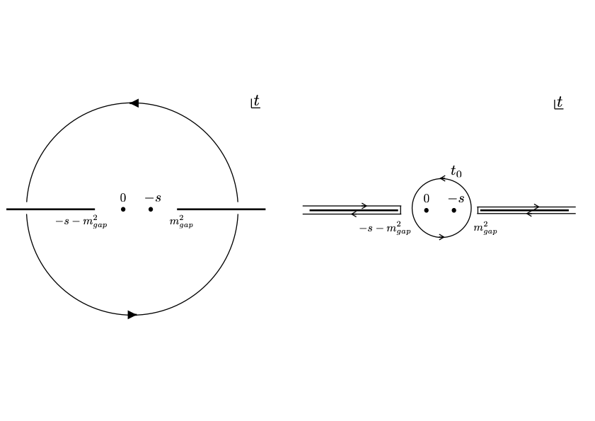
Figure 7: The vanishing of the arc integral at infinity on the left panel, cf. (121), can be restated as an equality of the integrals on the right panel (see (122).)

We evaluate the LHS of Eq. (122) using the low-energy expansion, and we use the RHS to establish some nontrivial properties that the coefficients of the low-energy expansion should satisfy. More precisely, we consider the expansion of (122) around $s=0$.

A few comments are in order. Firstly, note that the minimal tree-level graviton-exchange term in $f(s,u)\sim{1\over stu}$ does not contribute to the sum rules of interest here, $B_{k\geq 2}^{+}(s)$. In particular, we are able to expand the sum rules in powers of $s$. Assuming a more stringent Regge bound, $B^{+}_{1}(s)$ can be studied Caron-Huot:2021rmr and used to bound various coefficients in terms of $G$. We do not consider this sum rule in the present paper. Secondly, the non-minimal coupling $\beta_{R^{3}}$ contributes to $B_{2}^{+}$ and we utilize this fact in Sect. VI.2 in order to bound $\beta_{R^{3}}$ in terms of other EFT data.

IV.5 The theory islands

What is the space of gravitational EFTs that admit a consistent UV completion? Answering this question nonperturbatively is a formidable task, but we can consider the simpler question of understanding perturbatively in $G$ possible consistent UV completions of gravity. It is in this spirit that in this paper we focus on the leading-order-in-$G$ correction to general relativity.

Imagine that we label all possible perturbatively consistent theories of gravity by an index $i$ so that the four-graviton scattering amplitudes in a given theory are given by the matrix $\mathcal{M}_{i}$ (see Eq. (100)). It is clear then that by taking a superposition of such amplitudes with non-negative coefficients we again get an amplitude that satisfies all the constraints discussed in the sections above

$$\mathcal{M}_{\text{theory}}=\sum_{i}c_{i}\mathcal{M}_{i},~{}~{}~{}~{}~{}c_{i}\geq 0\,.$$ (123)

By expanding such amplitudes at low energies, as in Sect. IV.1, we get a set of higher-derivative corrections. The low-energy Wilson coefficients then form a convex cone which we can think of as the theory space, which is generated by vectors $\mathcal{M}_{i}$.

It has been recently established that causality, crossing and unitarity constrain Wilson coefficients both from above and from below Tolley:2020gtv ; Caron-Huot:2020cmc ; Arkani-Hamed:2020blm ; Sinha:2020win . In the space of couplings formed by weakly-coupled theories it is thus natural to talk about the theory island, namely the region spanned by known perturbative UV completions of gravity. By definition we have

$$\text{Theory island}\subseteq\text{EFThedron},$$ (124)

where by the EFThedron we call the set of amplitudes satisfying the constraints reviewed in this section (in particular we only impose perturbative unitarity). It is interesting to ask to what extent we can populate the space of allowed couplings by known perturbative UV completions. Recall that by a perturbative UV completion we call an $S$-matrix that satisfies unitarity, causality and crossing perturbatively in Newton’s constant $G$ and for any process $m\to n$.

There are two classes of perturbative UV completions we consider here: tree-level corrected theories and one-loop corrected theories. In tree-level corrected theories the leading-order correction to general relativity enters at tree-level, in other words the higher-derivative corrections in the Lagrangian are suppressed by a new scale, e.g. string scale, which can be much lower than the Planck scale. Perturbative string theories are famous examples of this type. It is a well-known fact that gravitational amplitudes in string theory have a great degree of universality, as discussed recently in Ref. Chowdhury:2019kaq . In Appendix B we review the cases of superstring, heterotic and bosonic strings at tree level. Alternatively, we can consider theories where the higher-derivative operators come with an extra power of $G$. The one-loop amplitudes computed in the present paper are precisely of this type. By choosing the mass spectrum and spins of the particles propagating in the loop we can get various amplitudes.

Combining these two examples we consider the following set of amplitudes in the present paper

$$\mathcal{M}_{\text{theory}}^{\text{here}}=c_{(\text{ss})}\mathcal{M}_{\text{tree}}^{(\text{ss})}+c_{(\text{hs})}\mathcal{M}_{\text{tree}}^{(\text{hs})}+c_{(\text{bs})}\mathcal{M}^{(\text{bs})}_{\text{tree}}+\sum_{S=0,{1\over 2},1,{3\over 2},2}c_{S}\mathcal{M}_{S}^{1-\text{loop}}\,.$$ (125)

Obviously, we do not claim that this space is complete. Let us emphasize that in the analysis below we allow taking arbitrary superpositions of string amplitudes with various tensions as well as one-loop amplitudes with arbitrary choices of the masses and spins, $S\leq 2$, of particles circulating in the loop.

On the string side, for example we can consider the $\epsilon$ deformation of the superstring amplitude discussed in the conclusions of Ref. Arkani-Hamed:2020blm . It is not clear however that these deformations can be promoted to fully consistent perturbative S-matrices. Moreover, we checked that adding this correction does not affect the theory island considered in the present paper in a noticeable way.

On the field-theory side we can consider gapped strongly-coupled theories of matter coupled to gravity. One interesting example is large-$N$ QCD coupled to gravity Kaplan:2020tdz . In this case we expect the tree-level corrections due to non-minimally coupled glueballs and one-loop corrections due to minimally-coupled glueballs to both enter at the same order $G^{2}$. Finally, we do not discuss here amplitudes in models with extra dimensions ArkaniHamed:1998rs ; Randall:1999ee ; Randall:1999vf . Of course, it would be very interesting to extend our analysis to include these examples as well.

In writing the contribution of matter we can imagine integrating out a multiple number of particles of given spin with various masses. For the constraints discussed below one can check that the effect of this freedom can be absorbed into rescaling of the coefficients $c_{S}$. In particular, the bounds that we describe below hold for any choice of masses and number of species for particles that we integrate out.

In the following sections we use these amplitudes to populate the theory island. Surprisingly, we find that

$$\text{Theory island}\ll\text{EFThedron}\,,$$ (126)

in a sense that should become clear below. In other words, the set of known weakly-coupled theories occupy a much smaller space in the space of couplings than is allowed by the general constraints coming from the analysis of $2\to 2$ scattering. This is, of course, in accord with the ongoing landscape vs swampland debate but is also different from that. Indeed, the theory island as defined here does not guarantee the existence of the nonperturbative completion of gravity. We only study the consistency of the leading-order corrections to the Einstein-Hilbert theory perturbatively in $G$ and already in this setting we seem to find a much smaller space of possibilities than follows from general constraints.

V Deriving bounds: elastic amplitude

In this section we analyze bounds on the low-energy expansion of the elastic amplitude $f(s,u)$ using the techniques of Ref. Arkani-Hamed:2020blm and Tolley:2020gtv ; Caron-Huot:2020cmc . We focus on couplings of the same dimensionality and derive two-sided bounds on them by explicitly identifying the facets of the relevant polytopes and then taking their crossing-symmetric section.

As observed in Ref. Arkani-Hamed:2020blm , identifying the relevant boundaries are particularly simple in case of the one-channel dispersion relations when the polytopes in question are cyclic. In case of the two-channel dispersion relations the cyclicity property is lost. However, as Ref. Arkani-Hamed:2020blm observed, a set of new boundaries that appear in this case involve low-spin partial waves and can be explicitly identified upon inspection. This is indeed what we observed in the examples below. To the best of our knowledge there is no proof that the list of boundaries obtained in this way is complete (and therefore that the bounds are optimal), and we do not attempt such a proof in the present work.

We will not attempt to relate couplings of different dimensionality to each other either. This problem was recently analyzed in Ref. Tolley:2020gtv ; Caron-Huot:2020cmc ; Sinha:2020win and the expected dimensional-analysis scaling of various couplings with order $\mathcal{O}(1)$ coefficients was rigorously established. It would be very interesting to apply these techniques to the gravitational amplitudes discussed here but we defer this to the future.

V.1 Strategy

We first briefly describe the basic strategy to derive bounds Arkani-Hamed:2020blm . We consider the vector of low-energy couplings of the same dimensionality $\vec{F}$ which via dispersion relations is given by the sum of $s$- and $u$-channel partial waves

$$\vec{F}=\sum_{J}\left(c_{J,s}\vec{V}_{J,s}+c_{J,u}\vec{V}_{J,u}\right),~{}~{}~{}~{}~{}c_{J,s},c_{J,u}\geq 0\,.$$ (127)

In this formula $c_{J,s}$ and $c_{J,u}$ encode spectral densities discussed in Sect. IV.2 and $\vec{V}_{J,s}$, $\vec{V}_{J,u}$ are known functions related to partial waves—see e.g. (134) for the precise formula. However for the present discussion we can simply think of $\vec{V}_{J,s}$ and $\vec{V}_{J,u}$ as some abstract, given vectors and $c_{J,s}$ , $c_{J,u}$ being non-negative numbers. We would like to characterize the space (127), which is a polytope. A convenient way to do it is by identifying its facets

$$\vec{F}\cdot\vec{W}_{i}\geq 0\,,$$ (128)

where $\vec{W}_{i}$ is a normal to a given facet. From Eq. (127) we see that all the facets are of the form

$$(W_{i})_{I_{0}}=\epsilon_{I_{0}I_{1}...I_{d}}V_{a_{1}}^{I_{1}}...V_{a_{d}}^{I_{d}}\,,$$ (129)

where we assumed that the vectors $\vec{V}_{a}$ are $(d+1)$-dimensional and we contracted them using the $(d+1)$-dimensional $\epsilon$-tensor. The index $a$ labels both spin and channel. Therefore, we can characterize the space (127) by a set of determinants $\langle F,a_{1},....,a_{d}\rangle\geq 0$. The task is then to find all $(a_{1},....,a_{d})$, such that Eq. (128) holds. In general, this is a formidable task since the space of vectors in Eq. (127) is infinite dimensional.

As explained in Ref. Arkani-Hamed:2020blm , remarkably, the set of vectors $\vec{V}_{J,s}$ defines a cyclic polytope, which for us simply means that the set of its boundaries can be written down explicitly very easily. They essentially take the form of determinants built out of pairs of consecutive vectors in the sum over spins. For example, for $d=4$ the relevant determinants take the form $(i,i+1,j,j+1)$ with $j>i$, where $i$ and $j$ label various spins in the sum (127).

The cyclicity property is lost when considering the sum of the $s$- and $u$-channel as in Eq. (127). By inspecting the resulting polytope Ref. Arkani-Hamed:2020blm observed that it is “almost cyclic” in the sense that the only boundaries which are not of the type $(i,i+1,j,j+1)$ in the example considered above involve low-spin partial waves in Eq. (127) and can be found by direct inspection. This is what we also find and this is the strategy of finding bounds that we follow in this paper. In particular, we do not prove that the set of bounds found in this way is complete (even though we suspect it to be the case). It would be very interesting to rigorously demonstrate this.

After the allowed region (128) is identified we impose crossing symmetry, which is the subspace defined by linear relations between various components of the coupling vector $\vec{F}$. By taking the crossing-symmetric slice of the allowed space of couplings we get two-sided bounds on the low-energy Wilson coefficients.

V.2 Non crossing-symmetric dispersive representation of low-energy couplings

Consider again the double-minus amplitude

$$\mathcal{M}_{4}(1^{-},2^{-},3^{+},4^{+})=(\langle 12\rangle[34])^{4}\ f(t,u)\,.$$ (130)

Following Ref. Arkani-Hamed:2020blm , we introduce the expansion

$$f(t,u)=f(t,-s-t)=\left(\frac{\kappa\hbox{}}{2}\right)^{2}{1\over stu}+|\beta_{R^{3}}|^{2}{tu\over s}-|\beta_{\phi}|^{2}{1\over s}+\sum_{k\geq j\geq 0}a_{k,j}s^{k-j}t^{j}\,.$$ (131)

From Eq. (131) we see that for fixed $k$ all $a_{k,j}$ have the same dimensionality. Crossing symmetry $f(t,u)=f(u,t)$ leads to linear relations among $a_{k,j}$ which will play an important role below.

Of course, in Eq. (98) we are expanding the same function, so the $f_{i,j}$ introduced there and the $a_{k,j}$ in Eq. (131) are all related to each other in a trivial fashion. We get for the first few coefficients

$$a_{0,0}=f_{0,0}\,,\hskip 34.14322pta_{1,0}=-f_{1,0}\,,\hskip 34.14322pta_{1,1}=0\,.$$ (132)

The vanishing of $a_{1,1}$ is a consequence of $t$–$u$ crossing symmetry of $f(t,u)$ which is not manifest in Eq. (131).

The function of interest $f(t,u)$ admits a simple dispersive representation

$$f(t,-s-t) =\oint{ds^{\prime}\over 2\pi i}{f(t,-s^{\prime}-t)\over s-s^{\prime}}=\left(\frac{\kappa\hbox{}}{2}\right)^{2}{1\over stu}+|\beta_{R^{3}}|^{2}{tu\over s}-|\beta_{\phi}|^{2}{1\over s}$$

$$\hbox{}\hskip 8.5359pt-\int_{m_{\rm gap}^{2}}^{\infty}{dm^{2}\over\pi}\biggl{(}\sum_{J=0}^{\infty}{1+(-1)^{J}\over 2}{\rho_{J}^{++}(m^{2})d_{0,0}^{J}(1+{2t\over m^{2}})\over m^{8}}{1\over s-m^{2}}$$

$$\hbox{}\hskip 113.81102pt+\sum_{J=4}^{\infty}{\rho_{J}^{+-}(m^{2})d_{4,4}^{J}\left(1+{2t\over m^{2}}\right)\over(t+m^{2})^{4}}{1\over-s-t-m^{2}}\biggr{)}\,.$$ (133)

In deriving (133) we used the Regge bound (120) to drop the arcs at infinity. When applied to Eq. (130) it implies that $|f(t,-s-t)|\leq{1/|s|}$ at large $s$ and fixed $t$. Indeed, this is the case for all the one-loop amplitudes that we consider.

An important feature of Eq. (133) is that crossing symmetry $f(t,u)=f(u,t)$ is not manifest (hence the title of this section). Therefore imposing it leads to interesting constraints. In fact, as we will see below it leads to two-sided bounds on the couplings.

By expanding Eq. (133) at small $s$ and $t$ we get the dispersive representations for the couplings $a_{k,j}$. They take the following form

$$\boxed{a_{k,j}=\int_{m_{\rm gap}^{2}}^{\infty}{dm^{2}\over\pi}{1\over(m^{2})^{k+1}}\left(\sum_{J=0}^{\infty}{1+(-1)^{J}\over 2}{\rho_{J}^{++}(m^{2})\over m^{8}}P_{++}^{j}({\cal J}^{2})+\sum_{J=4}^{\infty}{\rho_{J}^{+-}(m^{2})\over m^{8}}P_{+-}^{k,j}({\cal J}^{2})\right),}$$ (134)

where we introduced the spin Casimir ${\cal J}^{2}=J(J+1)$. We call Eq. (134) the dispersive representation of low-energy couplings. We again emphasize that crossing symmetry leads to linear relations among $a_{k,j}$ which are not manifest in Eq. (134).

In the formula above we introduced polynomials $P_{++}^{j}({\cal J}^{2})$ and $P_{+-}^{k,j}({\cal J}^{2})$ which have the following properties

$$P_{++}^{0}({\cal J}^{2}) =1\,,\qquad P_{+-}^{k,0}({\cal J}^{2})=(-1)^{k}\,,$$

$$P_{++}^{1}({\cal J}^{2}) ={\cal J}^{2}\,,\qquad P_{+-}^{k,1}({\cal J}^{2})=(-1)^{k+1}({\cal J}^{2}-20-k)\,,$$

$$\lim_{J\to\infty}P_{++}^{j}({\cal J}^{2}) ={1\over\Gamma(j+1)^{2}}J^{2j}+\ldots\,,\qquad\lim_{J\to\infty}P_{+-}^{k,j}({\cal J}^{2})={(-1)^{k+j}\over\Gamma(j+1)^{2}}J^{2j}+\ldots\,.$$ (135)

Based on the formulas above we see that couplings $a_{k,j}$ written in Eq. (134) roughly probe the $k$’th moment of the spectral density with respect to $m^{2}$ and $(2j)$’th moment with respect to spin. In particular, we expect that higher-$j$ coefficients to be more sensitive to higher-spin spectral densities and higher-$k$ couplings to have the large ${m^{2}\over m_{\rm gap}^{2}}$ region more suppressed. This is indeed what we will find in the explicit examples below.

Crossing symmetry leads to the set of sum rules which were dubbed null constraints in Ref. Caron-Huot:2020cmc . Effectively, they express the low-spin partial-wave data in terms of the higher-spin data. Consider for example the relation $a_{1,1}=0$, listed in Eq. (132). Using the formulas above we can write it as follows

$$\int_{m_{\rm gap}^{2}}^{\infty}{dm^{2}\over(m^{2})^{2}}{\rho_{4}^{+-}(m^{2})\over m^{8}}=\int_{m_{\rm gap}^{2}}^{\infty}{dm^{2}\over(m^{2})^{2}}\left(\sum_{J=2}^{\infty}{1+(-1)^{J}\over 2}{\rho_{J}^{++}(m^{2})\over m^{8}}{\cal J}^{2}+\sum_{J=5}^{\infty}{\rho_{J}^{+-}(m^{2})\over m^{8}}({\cal J}^{2}-21)\right),$$ (136)

where all the terms in the RHS of Eq. (136) are non-negative. In other words, crossing symmetry allows us to express the moment of $\rho_{4}^{+-}(m^{2})$ in terms of all other spectral densities.

Let us next describe the first few bounds for $k\leq 6$. We do not attempt to derive the bounds across the couplings of different dimensionalities as it was done in Ref. Tolley:2020gtv ; Caron-Huot:2020cmc ; Sinha:2020win ; Caron-Huot:2021rmr . Instead we focus on the geometry of couplings of the same dimensionality as was studied in Ref. Arkani-Hamed:2020blm . For $k=1,3,5$ we do not get any nontrivial bounds. For even $k$ the results are presented below.

${\bf k=0\!:}$

We first start with $k=0$. From (133) it immediately follows that

$$a_{0,0}\geq 0\,.$$ (137)

Moreover, we have

$$a_{k,0}={1\over\pi}\int_{m_{\rm gap}^{2}}^{\infty}{dm^{2}\over m^{2k+10}}\left(\sum_{J=0}^{\infty}{1+(-1)^{J}\over 2}\rho_{J}^{++}(m^{2})+(-1)^{k}\sum_{J=4}^{\infty}\rho_{J}^{+-}(m^{2})\right).$$ (138)

This immediately implies that $a_{k,0}$ for even $k$ can be interpreted as even moments $\mu_{k}$

$$\mu_{k}\equiv{1\over\pi}\int_{m_{\rm gap}^{2}}^{\infty}{dm^{2}\over m^{2k+10}}\left(\sum_{J=0}^{\infty}{1+(-1)^{J}\over 2}\rho_{J}^{++}(m^{2})+\sum_{J=4}^{\infty}\rho_{J}^{+-}(m^{2})\right).$$ (139)

As a result the bounds of Ref. Bellazzini:2020cot apply. For odd $k$, we obviously have $|a_{k}|\leq\mu_{k}$.

${\bf k=2\!:}$

Next consider $k=2$. Here the couplings of the same dimensionality are ${\bf a}_{2}=(a_{2,0},a_{2,1},a_{2,2})$. One obvious constraint is

$$a_{2,0}\geq 0\,.$$ (140)

On top of that we get the following list of constraints which specify the boundary of the region of allowed couplings,

$$\{\langle{\bf a}_{2},i_{s},i_{s}+2\rangle_{i_{s}\geq 2}\,,\hskip 28.45274pt\langle{\bf a}_{2},(i_{u}+1)^{(2)},i_{u}^{(2)}\rangle_{i_{u}\geq 4}\,,\hskip 28.45274pt\langle{\bf a}_{2},4_{u}^{(2)},2_{s}\rangle\}\geq 0\,.$$ (141)

Here we follow the notation of Ref. Arkani-Hamed:2020blm , which is defined as

$$\langle{\bf a}_{2},i,j\rangle\equiv\det\begin{pmatrix}a_{2,0}&v_{i,0}&v_{j,0}\\ a_{2,1}&v_{i,1}&v_{j,1}\\ a_{2,2}&v_{i,2}&v_{j,2}\end{pmatrix},$$ (142)

where we also define the following vectors

$$v_{J,m}^{(s)}=(J_{s})_{m} \equiv{1\over m!}\partial_{t}^{m}d^{0,0}_{J}(1+2t)|_{t=0}\,,$$ (143)

$$v_{J,k,m}^{(u)}=(J_{u}^{(k)})_{m} \equiv{1\over m!}\partial_{t}^{m}{1\over(k-m)!}\partial_{s}^{k-m}{1\over(1+s+t)}{d^{4,4}_{J}\left(1+2t\right)\over(1+t)^{4}}|_{s,t=0}\,,$$ (144)

where in the formula above we set the arbitrary mass scale $m^{2}=1$ since it leads to trivial overall rescaling of the vectors that enter into the determinant (142) and as such does not affect the positivity bounds (141). Note that the vector $v_{i,k}^{(u)}$ depends on the order $k$ of the corrections that we are studying, which we denote by $i_{u}^{(k)}$. For example, to evaluate (141) we should set $k=2$ in Eq. (144). The constraints (141) have an intuitive explanation. By plugging the dispersive representation of the couplings into the determinant $\langle{\bf a}_{2},i,j\rangle$ we get a sum over partial waves where the coefficients of partial wave $i$ and $j$ are zero. The plane $\langle{\bf a}_{2},i,j\rangle$ then separates the region in the coupling space where these coefficients are positive and negative.

We see that Eq. (141) involves cyclic constraints from the $s$-channel $\langle{\bf a}_{2},i_{s},i_{s}+2\rangle_{i_{s}\geq 2}$, similarly from the $u$-channel $\langle{\bf a}_{2},(i_{u}+1)^{(2)},i_{u}^{(2)}\rangle_{i_{u}\geq 4}$, as well as a mixed constraint $\langle{\bf a}_{2},4_{u}^{(2)},2_{s}\rangle$ that involves low-spin partial waves. This phenomenon observed in Ref. Arkani-Hamed:2020blm continues to hold for higher $k$ as well. It allows us to easily identify the set of conditions that carve out the region of allowed couplings analytically rather straightforwardly by inspecting the low-spin boundaries. Of course, in practice we only look for possible boundaries up to some finite spin $J_{{\rm max}}$ and assume that the observed pattern continues all the way to $J_{{\rm max}}=\infty$.

In deriving the bounds above we did not impose crossing symmetry. At the level $k=2$ we are working it implies that

$$\text{Crossing}:~{}~{}~{}a_{2,1}=a_{2,2}\,.$$ (145)

Taking the crossing-symmetric slice of the constraints (141) gives the two-sided bound on the Wilson coefficients

$$-{90\over 11}\leq{a_{2,1}\over a_{2,0}}={a_{2,2}\over a_{2,0}}\leq 6\,.$$ (146)

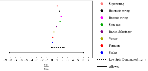
Figure 8: The allowed region for ${a_{2,1}\over a_{2,0}}$ given by Eq. (146) is depicted in black. The explicit amplitudes that emerge from integrating out the one-loop matter or tree-level string theories are depicted in various colors. Assuming LSD in the form (152) with $\alpha=10^{2}$ one can derive stronger bounds which we depict by the dashed line.

It is very striking that for the explicit UV completions studied here we find a much narrow window of possibilities that we depict in Fig. 8. We now try to understand the origin of this fact. To do this it will be useful to use the null constraint $a_{2,1}-a_{2,2}=0$ to derive a bound similar to Eq. (146). By adding the null constraint to the dispersive representations for $a_{2,1}$ and $a_{2,2}$ it is straightforward to show that

$$-{108\over 13}{\langle\rho_{5}^{+-}\rangle_{2}\over\langle\rho_{0}^{++}\rangle_{2}+\langle\rho_{4}^{+-}\rangle_{2}+\langle\rho_{5}^{+-}\rangle_{2}}\leq{a_{2,1}\over a_{2,0}}={a_{2,2}\over a_{2,0}}\leq{6\langle\rho_{2}^{++}\rangle_{2}+{16\over 7}\langle\rho_{4}^{+-}\rangle_{2}\over\langle\rho_{0}^{++}\rangle_{2}+\langle\rho_{4}^{+-}\rangle_{2}+\langle\rho_{2}^{++}\rangle_{2}}\,,$$ (147)

where we introduced $\langle\ldots\rangle$ for the relevant integrals over intermediate energies $m^{2}$

$$\langle\rho_{J}\rangle_{k}\equiv{1\over\pi}\int_{m_{\rm gap}^{2}}^{\infty}{dm^{2}\over m^{2k+10}}\rho_{J}(m^{2})\,.$$ (148)

To derive the upper bound in Eq. (147) we used the dispersive representation for $a_{2,1}-{2\over 7}(a_{2,2}-a_{2,1})$. To derive the lower bound we considered $a_{2,1}+{4\over 13}(a_{2,2}-a_{2,1})$.

The bound (147) is rigorous. Its advantage however is that it only contains low-spin spectral densities. By adding the null constraint $a_{2,1}-a_{2,2}=0$ with an appropriate coefficient we made sure that all the higher-spin contributions are sign-definite and the bound (147) then follows. It is clear then how can we come close to the saturation of the bounds (146). The upper bound saturation requires that $\langle\rho_{2}^{++}\rangle_{2}$ is dominant, whereas the lower-bound saturation requires that $\langle\rho_{5}^{+-}\rangle_{2}$ dominates. Note that each of these is not the minimal spin that appears in the corresponding channel, which are $\langle\rho_{0}^{++}\rangle_{2}$ and $\langle\rho_{4}^{+-}\rangle_{2}$ correspondingly.

This is not what happens in the known physical theories as we will show in more detail. In the examples that we analyze in this paper the higher-spin contributions to the spectral densities are suppressed compared to the minimal spin ones. The fact that at large spin the spectral densities decay exponentially in spin is something familiar from the fact that the scattering is local in the impact parameter space. Analyzing the concrete examples we see that this hierarchy continues all the way to minimal spin. We call this phenomenon low-spin dominance (LSD) of partial wave and mathematically we can express it as follows:

$$\text{Low-spin dominance (weak)}:~{}~{}~{}\langle\rho_{4}^{+-}\rangle_{k} \geq\langle\rho_{J>4}^{+-}\rangle_{k},~{}~{}~{}\langle\rho_{0}^{++}\rangle_{k}\geq\langle\rho_{J>0}^{++}\rangle_{k}\,.$$ (149)

In fact, Eq. (149) is very conservative and in the explicit examples the suppression of higher-spin partial waves is much stronger than Eq. (149). Nevertheless, already using Eqs. (149) and (147) we can strengthen the bound (146) to obtain

$$\eqref{eq:rigorouslow}+\eqref{eq:lowspindom}:~{}~{}~{}-{54\over 13}\leq{a_{2,1}\over a_{2,0}}={a_{2,2}\over a_{2,0}}\leq 3\,.$$ (150)

We clarify that here we derived Eq. (150) to illustrate the point that LSD implies stronger bounds. We have not tried to find the optimal bound that follows from Eq. (149) and dispersive representations of the couplings. It would be interesting to study this more systematically.

It is also instructive to see what happens if we assume LSD in the strong form

$$\text{Low-spin dominance (strong)}:~{}~{}~{}\langle\rho_{4}^{+-}\rangle_{k} \gg\langle\rho_{J>4}^{+-}\rangle_{k},~{}~{}~{}\langle\rho_{0}^{++}\rangle_{k}\gg\langle\rho_{J>0}^{++}\rangle_{k}\,.$$ (151)

We will discuss in more detail the expected form of the hierarchy below in the section dedicated to spectral densities, but for now it is sufficient to say that we will find that Eq. (151) correctly captures the region occupied by the known theories. To make (151) more precise let us introduce its quantitative version

$$\text{Low-spin dominance ($\alpha$-factor)}:~{}~{}~{}\langle\rho_{4}^{+-}\rangle_{k} \geq\alpha\langle\rho_{J>4}^{+-}\rangle_{k},~{}~{}~{}\langle\rho_{0}^{++}\rangle_{k}\geq\alpha\langle\rho_{J>0}^{++}\rangle_{k}\,.$$ (152)

For illustrating bounds, below we choose for concreteness $\alpha=10^{2}$. This choice is not accidental as the perturbative examples considered in this paper, tree-level string amplitudes and one-loop matter amplitudes, happen to be of this type.

Let us now consider the bounds coming from Eq. (147) with the additional assumption of $\alpha=10^{2}$ LSD (152). In this way we obtain

$$\eqref{eq:rigorouslow}+\eqref{eq:lowspindomAlpha}|_{\alpha=10^{2}}:~{}~{}~{}-0.083\leq{a_{2,1}\over a_{2,0}}={a_{2,2}\over a_{2,0}}\leq 2.286\,.$$ (153)

It is also interesting to consider what happens if we consider $\alpha\to\infty$. In this case one can again use the trick of adding a null constraint $(a_{2,2}-a_{2,1})$ with some non-zero coefficient to dispersive representation of the couplings to show that

$$\text{LSD}_{\alpha\to\infty}:~{}~{}~{}0\leq{a_{2,1}\over a_{2,0}}={a_{2,2}\over a_{2,0}}\leq 2\,.$$ (154)

Remarkably, we find that the region occupied by known theories in Fig. 8 lies inside Eq. (153) and even Eq. (154). We will see below that the phenomenon of the data being well explained by the strong version of LSD continues for higher $k$’s as well.

${\bf k=4\!:}$

For $k=4$ we first consider a subset of couplings ${\bf\hat{a}_{4}}=(a_{4,0},a_{4,1},a_{4,2})$. From the dispersive representation of the couplings it immediately follows that

$$a_{4,0}\geq 0\,.$$ (155)

Analyzing the sums over the partial waves we get the following list of constraints

$$\bigl{\{}\langle{\bf\hat{a}}_{2},i_{s},i_{s}+2\rangle_{i_{s}\geq 2}\,,~{}~{}\langle{\bf\hat{a}}_{4},i_{u}^{(4)}+1,i_{u}^{(4)}\rangle_{i_{u}\geq 5}\,,~{}~{}\langle{\bf\hat{a}}_{4},5_{u}^{(4)},2_{s}\rangle\bigr{\}}\geq 0\,.$$ (156)

These include the usual cyclic constraints, as well as an extra fixed constraint. We plot the allowed region in the as shaded (green) in Fig. 9. A characteristic feature of the allowed region is that it is unbounded.

In deriving the bounds above we have not used crossing symmetry which leads to improved two-sided bounds. To do that we can consider a complete set of couplings at $k=4$, namely ${\bf a_{4}}=(a_{4,0},a_{4,1},a_{4,2},a_{4,3},a_{4,4})$. It is then straightforward to check by inspection that the following set of constraints define the boundary region in the space of couplings:

$$\bigl{\{} \langle{\bf a}_{4},i_{s},i_{s}+2,j_{s},j_{s}+2\rangle_{j>i\geq 2}\,,~{}~{}\langle{\bf a}_{4},i_{u}^{(4)},i_{u}^{(4)}+1,j_{u}^{(4)},j_{u}^{(4)}+1\rangle_{j>i\geq 5}\,,$$

$$\langle{\bf a}_{4},i_{s},i_{s}+2,j_{u}^{(4)}+1,j_{u}^{(4)}\rangle_{i\geq 4,j\geq 5}\,,~{}~{}\langle{\bf a}_{4},2_{s},4_{s},j_{u}^{(4)}+1,j_{u}^{(4)}\rangle_{j\geq 7}\,,$$

$$\langle 2_{s},{\bf a}_{4},i_{s},i_{s}+2,5^{(4)}_{u}\rangle_{i\geq 4}\,,~{}~{}\langle 5_{u}^{(4)},{\bf a}_{4},j_{u}^{(4)},j_{u}^{(4)}+1,2_{s}\rangle_{j\geq 7}\,,$$

$$\langle{\bf a}_{4},4_{u}^{(4)},5_{u}^{(4)},6_{u}^{(4)},7_{u}^{(4)}\rangle\,,~{}~{}\langle{\bf a}_{4},2_{s},4_{s},4_{u}^{(4)},5_{u}^{(4)}\rangle,\langle{\bf a}_{4},2_{s},4_{s},7_{u}^{(4)},4_{u}^{(4)}\rangle\,,$$

$$\langle{\bf a}_{4},4_{u}^{(4)},5_{u}^{(4)},7_{u}^{(4)},2_{s}\rangle\,,\langle 4_{u}^{(4)},{\bf a}_{4},5_{u}^{(4)},6_{u}^{(4)},4_{s}\rangle,\langle 4_{u}^{(4)},{\bf a}_{4},6_{u}^{(4)},7_{u}^{(4)},4_{s}\rangle\bigr{\}}\geq 0\,.$$ (157)

It is easy to recover the previous constraints (156) from Eq. (V.2) by taking some of the spins to infinity. For example $\lim_{i_{s}\to\infty}\langle 2_{s},{\bf a}_{4},i_{s},i_{s}+2,5^{(4)}_{u}\rangle_{i\geq 4}\geq 0$ reduces to $\langle{\bf\hat{a}}_{4},5_{u}^{(4)},2_{s}\rangle\geq 0$.

A somewhat new feature of this case compared to the ones considered above that mixed $s$–$u$ channel boundaries come in infinite families. However, these families are again either cyclic, as in $\langle{\bf a}_{4},i_{s},i_{s}+2,j_{u}^{(4)}+1,j_{u}^{(4)}\rangle_{i\geq 4,j\geq 5}$ or involve low-spin partial wave only and therefore easily identifiable. We find it quite remarkable that the allowed region can be found analytically!

We then consider the section of this region by the crossing symmetry relations that take the form

$$\text{Crossing}:~{}~{}~{}a_{4,3}=2(a_{4,2}-a_{4,1})\,,~{}~{}~{}~{}~{}a_{4,4}=a_{4,2}-a_{4,1}\,.$$ (158)

As a result we get the region of allowed couplings depicted in red in Fig. 9. To generate the plot we considered bounds (V.2) where we truncated the maximal spin to $i_{\rm max},j_{\rm max},k_{\rm max}=20$. We also checked explicitly that the all determinants obtained in this way are non-negative given dispersive representation for the couplings truncated to $J_{\rm max}=200$.

The bounds coming from imposing Eq. (V.2) together with crossing symmetry (158) are two-sided, both from above and from below. The theory island occupied by the known theories forms a tiny black slit inside the allowed region.

As we did for $k=2$ we can again understand the structure of the island using the idea of LSD. To this extent we can use the null constraints coming from crossing (158) to derive the following rigorous bounds

$$-{7.01\langle\rho_{5}^{+-}\rangle_{4}+20.18\langle\rho_{6}^{+-}\rangle_{4}\over\langle\rho_{0}^{++}\rangle_{4}+\langle\rho_{4}^{+-}\rangle_{4}+\langle\rho_{5}^{+-}\rangle_{4}+\langle\rho_{6}^{+-}\rangle_{4}}\leq {a_{4,1}\over a_{4,0}}\leq{6\langle\rho_{2}^{++}\rangle_{4}+20\langle\rho_{4}^{++}\rangle_{4}+4.01\langle\rho_{4}^{+-}\rangle_{4}\over\langle\rho_{0}^{++}\rangle_{4}+\langle\rho_{4}^{+-}\rangle_{4}+\langle\rho_{2}^{++}\rangle_{4}+\langle\rho_{4}^{++}\rangle_{4}}\,,$$ (159)

$$-{20.16\langle\rho_{5}^{+-}\rangle_{4}\over\langle\rho_{0}^{++}\rangle_{4}+\langle\rho_{4}^{+-}\rangle_{4}+\langle\rho_{5}^{+-}\rangle_{4}+\langle\rho_{6}^{+-}\rangle_{4}}\leq {a_{4,2}\over a_{4,0}}$$

$$\hskip-56.9055pt\leq{6\langle\rho_{2}^{++}\rangle_{4}+90\langle\rho_{4}^{++}\rangle_{4}+6.43\langle\rho_{4}^{+-}\rangle_{4}+15.32\langle\rho_{6}^{+-}\rangle_{4}\over\langle\rho_{0}^{++}\rangle_{4}+\langle\rho_{4}^{+-}\rangle_{4}+\langle\rho_{2}^{++}\rangle_{4}+\langle\rho_{4}^{++}\rangle_{4}+\langle\rho_{6}^{+-}\rangle_{4}}\,.$$ (160)

Again we see that the corners of the red regions in Fig. 9 can be obtained from Eq. (159) by assuming that the sub-leading spins in the corresponding channels are dominant. This is not what happens in the physical theories and again assuming weak LSD (149) we can get a tighter bounds in which physical theories reside. In practice, we see that physical theories occupy even smaller region which can be understood using the strong version of LSD (151).

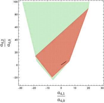
Figure 9: The allowed region for $({a_{4,1}\over a_{4,0}},{a_{4,2}\over a_{4,0}})$. The lightly shaded (green) region corresponds to the bounds (156). The darkly shaded (red) region corresponds to the bounds (V.2). The black theory island (which is so narrow that on this scale it looks like a line segment) is the region covered by known amplitudes. The small gray-shaded region that surrounds the black theory island corresponds to the LSD $\alpha=10^{2}$ bounds.

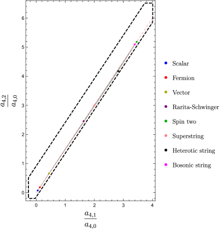
Figure 10: A scaled version of the theory island from Fig. 9. The dashed black line bounds the region which is found from Eqs. (159) and (161) using the LSD assumption (152) with $\alpha=10^{2}$. The dashed red line $a_{4,2}={3\over 2}a_{4,1}$ corresponds to $\alpha=\infty$ bound (164). Remarkably, all known theories lie in this small region where they populate a small region around the $\alpha=\infty$ curve.

A striking feature of Fig. 10 is that the known theories align closely with the straight line with the slope ${3/2}$. To understand this we can derive the bound analogous to Eq. (159) for the difference $a_{4,2}-{3\over 2}a_{4,1}$. It takes the following form

$$-{3\langle\rho_{2}^{++}\rangle_{4}+15\langle\rho_{5}^{+-}\rangle_{4}\over\langle\rho_{0}^{++}\rangle_{4}+\langle\rho_{4}^{+-}\rangle_{4}+\langle\rho_{2}^{++}\rangle_{4}+\langle\rho_{5}^{+-}\rangle_{4}}\leq {a_{4,2}-{3\over 2}a_{4,1}\over a_{4,0}}\leq{60\langle\rho_{4}^{++}\rangle_{4}+0.47\langle\rho_{4}^{+-}\rangle_{4}+45.58\langle\rho_{6}^{+-}\rangle_{4}\over\langle\rho_{0}^{++}\rangle_{4}+\langle\rho_{4}^{+-}\rangle_{4}+\langle\rho_{4}^{++}\rangle_{4}+\langle\rho_{6}^{+-}\rangle_{4}}\,.$$ (161)

We emphasize that at this point the bound (161) is rigorous and no additional assumptions have been made. To derive an upper bound we have considered the dispersive representation for $a_{4,2}-{3\over 2}a_{4,1}+{1687\over 7205}(a_{4,3}-2a_{4,4})+{411\over 524}(a_{4,3}-2(a_{4,2}-a_{4,1}))$, where we made use of crossing (158). The lower bound follows directly from the dispersive representation of $a_{4,2}-{3\over 2}a_{4,1}$.

To make use of it, we can now assume $\alpha=10^{2}$ LSD and apply it to the bounds (159) and (161). In this way we get

$$\eqref{eq:boundsk4lowspin}+\eqref{eq:boundsk4lowspin2}+\eqref{eq:differenceboundk4}+\text{LSD}_{\alpha=10^{2}}:~{}~{}~{}-0.27\leq {a_{4,1}\over a_{4,0}}\leq 4.01,$$ (162)

$$-0.20\leq {a_{4,2}\over a_{4,0}}\leq 6.52,$$

$$-0.15\leq {a_{4,2}-{3\over 2}a_{4,1}\over a_{4,0}}\leq 0.92.$$ (163)

We plot the result in Fig. 10 and again observe that the known examples neatly land in the predicted region. Moreover, it is straightforward to see that if we increase $\alpha$ the bound (161) becomes not optimal and instead we get

$$\text{LSD}_{\alpha\to\infty}:~{}~{}~{}~{}{a_{4,2}-{3\over 2}a_{4,1}\over a_{4,0}} =0,~{}~{}~{}~{}0\leq{a_{4,1}\over a_{4,0}}\leq 4,~{}~{}~{}~{}0\leq{a_{4,2}\over a_{4,0}}\leq 6\,.$$ (164)

which is the line along which our explicit examples cluster. Intuitively, this result can be understood as follows: We write down explicitly the dispersive representation for the couplings $a_{4,i}$,

$$a_{4,0} =\int_{m_{\rm gap}^{2}}^{\infty}{dm^{2}\over\pi}{\rho_{++0}(m^{2})\over(m^{2})^{9}}+\int_{m_{\rm gap}^{2}}^{\infty}{dm^{2}\over\pi}{\rho_{+-4}(m^{2})\over(m^{2})^{9}}+{\rm higher\ spin}\,,\hskip 56.9055pt\hbox{}$$

$$a_{4,1} =4\int_{m_{\rm gap}^{2}}^{\infty}{dm^{2}\over\pi}{\rho_{+-4}(m^{2})\over(m^{2})^{9}}+{\rm higher\ spin}\,,$$

$$a_{4,2} =6\int_{m_{\rm gap}^{2}}^{\infty}{dm^{2}\over\pi}{\rho_{+-4}(m^{2})\over(m^{2})^{9}}+{\rm higher\ spin}\,,$$ (165)

where ‘higher spin’ denotes infinitely many partial-wave contributions. Suppose that the lowest-spin partial waves in each channel dominates. Note that the leading spin $J=0$ contribution in the $\rho_{++J}$ channel drops out from $a_{4,1}$ and $a_{4,2}$. Notice that if we set the ‘higher-spin’ terms to $0$ in the formulas above we get the region (164). A priori it is not clear that this follows from sending $\alpha\to\infty$ in Eq. (152) since we still have infinitely many spins that can potentially compensate for the smallness of $1/\alpha$. Crossing symmetry, however, guarantees that it is indeed the case and higher-spin contributions cannot compensate for smallness of $1/\alpha$ as can be seen from the explicit analysis using the finite number of partial-wave bounds similar to Eq. (161).

Note that there are two distinct ways in which points can be close to the straight line in Fig. 10. First, as explained above by assuming the strong version of LSD in $a_{4,1}$ and $a_{4,2}$. Another mechanism is to have $a_{4,0}\gg a_{4,1},a_{4,2}$ which happens when the contribution of $\rho_{++0}$ to $a_{4,0}$ dominates over the partial waves that enter to $a_{4,1}$ and $a_{4,2}$. In this case the points appear very close to the origin on the $({a_{4,1}\over a_{4,0}},{a_{4,2}\over a_{4,0}})$ plot and the slope defined by the ratio ${a_{4,2}\over a_{4,1}}$ is not directly visible, nor does it need to be ${3\over 2}$. In fact, $a_{4,1}$ and $a_{4,2}$ have nontrivial higher-spin corrections in Eq. (165), i.e. $\rho^{++}_{2}$ is sizable compared to $\rho^{+-}_{4}$ and contributes ruining the $3/2$ ratio for ${a_{4,2}\over a_{4,1}}$. This is precisely what happens for the scalar and fermion contributions in Fig. 10. In this case, by looking at Fig. 10 it is not apparent that Eq. (165) is not an accurate description of these points since they are close to the origin, which is on the line. When this happens the simple model of dropping higher-spin contributions in Eq. (165) is too crude. For example, consider the one-loop massive scalar amplitude which lies very close to the origin in Fig. 10. In this case to accurately capture $a_{4,1}$ we also need to include $\rho^{++}_{2}(m^{2})$ (which is comparable to $\rho^{+-}_{4}(m^{2})$ in this case) in the formulas (165). For $a_{4,2}$ to get $1\%$ precision $\rho^{++}_{4}(m^{2})$ required as well. We re-iterate that in deriving the bounds using LSD we did not make any assumptions about the contributions of infinitely many higher-spin terms in Eq. (165) and instead used crossing symmetry to derive rigorous and tight bounds based on Eq. (152). In contrast, when we use Eq. (165) and try to estimate the contribution of higher-spin partial waves we observe that depending on the model and the coupling at hand, the number of terms required to be kept in the expansion to reach good precision varies.

We observe that the relation (164) generates a hierarchy $\sim 10^{-2}$ between certain coefficients in the low-energy EFT. A naive low-energy observer could have been puzzled by the fact that $|a_{4,2}-{3\over 2}a_{4,1}|\ll a_{4,0}$. We see that this hierarchy is generated by unitarity, namely it appears due to the dominance of the dispersive integrals by the low-spin partial waves. We discuss this point further in Sect. V.5.

${\bf k=6\!:}$

The analysis gets more and more complicated as we go to higher $k$. For $k=6$ we get the $7$-dimensional coupling vector ${\bf a_{6}}=(a_{6,0},a_{6,1},a_{6,2},a_{6,3},a_{6,4},a_{6,5},a_{6,6})$. Out of seven couplings only four are independent due to the crossing-symmetry relations

$$\text{Crossing}:~{}~{}~{}a_{6,4} =5(a_{6,1}-a_{6,2})+3a_{6,3}\,,$$

$$a_{6,5} =6(a_{6,1}-a_{6,2})+3a_{6,3}\,,$$

$$a_{6,6} =2(a_{6,1}-a_{6,2})+a_{6,3}\,.$$ (166)

Working out the boundary of the coupling region is more laborious, but follows the same pattern that we observed before

$$\bigl{\{} \langle{\bf a}_{6},i_{s},i_{s}+2,j_{s},j_{s}+2,k_{s},k_{s}+2\rangle_{k>j>i\geq 2}\,,$$

$$\langle{\bf a}_{6},i_{u}^{(6)}+1,i_{u}^{(6)},j_{u}^{(6)},j_{u}^{(6)}+1,k_{u}^{(6)},k_{u}^{(6)}+1\rangle_{k>j>i\geq 5}\,,$$

$$\langle{\bf a}_{6},5_{u}^{(6)},4_{u}^{(6)},6_{u}^{(6)},7_{u}^{(6)},8_{u}^{(6)},9_{u}^{(6)}\rangle\,,~{}~{}~{}\text{mixed $s$--$u$ constraints}\bigr{\}}\geq 0\,,$$ (167)

where we list the explicit mixed constraints that we found in Appendix C. After the boundaries are identified we take the crossing-symmetric slice (V.2). The resulting region of allowed couplings is plotted in Fig. 11. The region covered by the known theories is again a small island in the space of couplings.

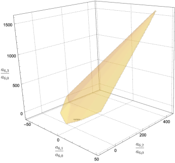
Figure 11: The allowed region for couplings $({a_{6,1}\over a_{6,0}},{a_{6,2}\over a_{6,0}},{a_{6,3}\over a_{6,0}})$ derived from constraints (V.2). The black little island (barely visible) is the space occupied by known perturbative amplitudes. The small gray shaded region that surrounds it corresponds to the LSD $\alpha=10^{2}$ bound. The details on how the plot was generated can be found in Appendix C.

As in the analysis above the island occupied by the explicit examples can be understood using the idea of strong LSD. As before the first step is to derive a set of rigorous bounds in terms of the low-spin partial waves. We do not present the complete analysis here but only present some of the relevant bounds

$$-{9\langle\rho_{2}^{++}\rangle_{6}+25\langle\rho_{5}^{+-}\rangle_{6}\over\langle\rho_{0}^{++}\rangle_{6}+\langle\rho_{4}^{+-}\rangle_{6}+\langle\rho_{2}^{++}\rangle_{6}+\langle\rho_{5}^{+-}\rangle_{6}}\leq {a_{6,2}-{5\over 2}a_{6,1}\over a_{6,0}}$$

$$\hbox{}\hskip-56.9055pt\leq{40\langle\rho_{4}^{++}\rangle_{6}+315\langle\rho_{6}^{++}\rangle_{6}+32.56\langle\rho_{6}^{+-}\rangle_{6}+220.41\langle\rho_{7}^{+-}\rangle_{6}\over\langle\rho_{0}^{++}\rangle_{6}+\langle\rho_{4}^{+-}\rangle_{6}+\langle\rho_{4}^{++}\rangle_{6}+\langle\rho_{6}^{++}\rangle_{6}+\langle\rho_{6}^{+-}\rangle_{6}+\langle\rho_{7}^{+-}\rangle_{6}}\,,$$ (168)

$$-{20\langle\rho_{2}^{++}\rangle_{6}+66.67\langle\rho_{5}^{+-}\rangle_{6}\over\langle\rho_{0}^{++}\rangle_{6}+\langle\rho_{4}^{+-}\rangle_{6}+\langle\rho_{2}^{++}\rangle_{6}+\langle\rho_{5}^{+-}\rangle_{6}}\leq {a_{6,3}-{10\over 3}a_{6,1}\over a_{6,0}}$$

$$\hbox{}\hskip-56.9055pt\leq{73.34\langle\rho_{4}^{++}\rangle_{6}+1540\langle\rho_{6}^{++}\rangle_{6}+163.49\langle\rho_{6}^{+-}\rangle_{6}+495.64\langle\rho_{7}^{+-}\rangle_{6}\over\langle\rho_{0}^{++}\rangle_{6}+\langle\rho_{4}^{+-}\rangle_{6}+\langle\rho_{4}^{++}\rangle_{6}+\langle\rho_{6}^{++}\rangle_{6}+\langle\rho_{6}^{+-}\rangle_{6}+\langle\rho_{7}^{+-}\rangle_{6}}.$$ (169)

From the formulas above and a similar analysis for $a_{6,i}$ we also see that

$$\text{LSD}_{\alpha\to\infty}:~{}~{}~{}~{}~{} {a_{6,2}-{5\over 2}a_{6,1}\over a_{6,0}}=0\,,~{}~{}~{}~{}~{}{a_{6,3}-{10\over 3}a_{6,1}\over a_{6,0}}=0\,,$$

$$0 \leq{a_{6,1}\over a_{6,0}}\leq 6\,,~{}~{}~{}~{}~{}0\leq{a_{6,2}\over a_{6,0}}\leq 15\,,$$

$$0 \leq{a_{6,3}\over a_{6,0}}\leq 20\,.$$ (170)

As for $k=4$ we can understood the result above by simply dropping higher-spin contributions in the dispersive representations for the couplings and keeping only the lowest-spin partial waves in each channel

$$a_{6,0} =\int_{m_{\rm gap}^{2}}^{\infty}{dm^{2}\over\pi}{\rho_{++0}(m^{2})\over(m^{2})^{11}}+\int_{m_{\rm gap}^{2}}^{\infty}{dm^{2}\over\pi}{\rho_{+-4}(m^{2})\over(m^{2})^{11}}+{\rm higher\ spin},$$ (171)

$$a_{6,1} =6\int_{m_{\rm gap}^{2}}^{\infty}{dm^{2}\over\pi}{\rho_{+-4}(m^{2})\over(m^{2})^{11}}+{\rm higher\ spin},$$ (172)

$$a_{6,2} =15\int_{m_{\rm gap}^{2}}^{\infty}{dm^{2}\over\pi}{\rho_{+-4}(m^{2})\over(m^{2})^{11}}+{\rm higher\ spin},$$ (173)

$$a_{6,3} =20\int_{m_{\rm gap}^{2}}^{\infty}{dm^{2}\over\pi}{\rho_{+-4}(m^{2})\over(m^{2})^{11}}+{\rm higher\ spin}.$$ (174)

We emphasize again that while dropping infinitely many terms is not justified, the bound (V.2) is rigorous.

Assuming the strong version of the LSD and using Eq. (V.2) we again find the small region around the island occupied by the explicit examples, as shown in Fig. 11 and Fig. 12.

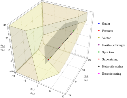
Figure 12: The scaled version of the theory island from Fig. 11. The gray region is derived using the bounds (V.2) (and similar bounds for $a_{6,i}$ which we do not write down explicitly) and the LSD assumption (152) with $\alpha=10^{2}$. The dashed black line ${a_{6,2}\over a_{6,1}}={5\over 2}$ and ${a_{6,3}\over a_{6,1}}={10\over 3}$ corresponds to $\text{LSD}_{\alpha\to\infty}$ bounds given in Eq. (V.2).

${\bf k=8\!:}$

For $k=8$ we do not perform the analysis of finding the allowed region but simply report on the data in the specific theories. There are five independent couplings at this level which we choose to be $a_{8,0\leq j\leq 4}$. Other couplings $a_{8,5\leq j\leq 8}$ can be obtained by crossing. The dispersive representation of the couplings take the following form

$$a_{8,0} =\int_{m_{\rm gap}^{2}}^{\infty}{dm^{2}\over\pi}{\rho_{++0}(m^{2})\over(m^{2})^{13}}+\int_{m_{\rm gap}^{2}}^{\infty}{dm^{2}\over\pi}{\rho_{+-4}(m^{2})\over(m^{2})^{13}}+{\rm higher\ spin}\,,$$

$$a_{8,1} =8\int_{m_{\rm gap}^{2}}^{\infty}{dm^{2}\over\pi}{\rho_{+-4}(m^{2})\over(m^{2})^{13}}+{\rm higher\ spin}\,,$$

$$a_{8,2} =28\int_{m_{\rm gap}^{2}}^{\infty}{dm^{2}\over\pi}{\rho_{+-4}(m^{2})\over(m^{2})^{13}}+{\rm higher\ spin}\,,$$

$$a_{8,3} =56\int_{m_{\rm gap}^{2}}^{\infty}{dm^{2}\over\pi}{\rho_{+-4}(m^{2})\over(m^{2})^{13}}+{\rm higher\ spin}\,,$$

$$a_{8,4} =70\int_{m_{\rm gap}^{2}}^{\infty}{dm^{2}\over\pi}{\rho_{+-4}(m^{2})\over(m^{2})^{13}}+{\rm higher\ spin}\,,$$ (175)

where we keep the leading spin contributions in both channels. To visualize the data we consider two 3-dimensional slices of the space of couplings with coordinates $({a_{8,1}\over a_{8,0}},{a_{8,2}\over a_{8,0}},{a_{8,3}\over a_{8,0}})$ and $({a_{8,2}\over a_{8,0}},{a_{8,3}\over a_{8,0}},{a_{8,4}\over a_{8,0}})$. Formulas (175) define a line in this space upon neglecting the higher-spin partial wave contributions. We depict the result in Fig. 13 and it is again completely analogous to our observations for lower $k$’s. It would be interesting to extend the analysis done for lower $k$ to this case as well.

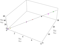
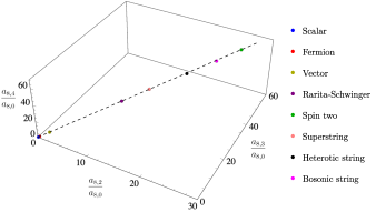
(a)	(b)

Figure 13: A plot for the data for $a_{8,j}$ in various theories. In panel a) we plot $({a_{8,1}\over a_{8,0}},{a_{8,2}\over a_{8,0}},{a_{8,3}\over a_{8,0}})$ and in panel b) $({a_{8,2}\over a_{8,0}},{a_{8,3}\over a_{8,0}},{a_{8,4}\over a_{8,0}})$. The dashed line corresponds to the low-spin dominant line defined by Eq. (175) upon neglecting the higher-spin contributions to the partial-wave expansion.

V.3 Crossing-symmetric dispersive representation of low-energy couplings

We can also analyze the same amplitude using dispersive representation with a different pair of channels. We start by recalling that

$$\mathcal{M}_{4}(1^{+},2^{-},3^{-},4^{+})=(\langle 23\rangle[14])^{4}\,f(s,u)\,.$$ (176)

We would like to use dispersion relations at fixed $t$ to derive the dispersive representation for the low-energy couplings. For this purpose it is natural to introduce the following parameterization of the low-energy expansion of $f(s,u)$

$$f(z-{t\over 2},-z-{t\over 2}) =\left(\frac{\kappa\hbox{}}{2}\right)^{2}{1\over t({t^{2}\over 4}-z^{2})}+|\beta_{R^{3}}|^{2}{({t^{2}\over 4}-z^{2})\over t}-|\beta_{\phi}|^{2}{1\over t}$$

$$\hskip 8.5359pt+\sum_{k\geq q\geq 0}^{\infty}\tilde{a}_{k,q}z^{k-q}t^{q},~{}~{}~{}~{}~{}z=s+{t\over 2},~{}~{}~{}~{}~{}k-q\in 2{\mathbb{Z}}_{\geq 0}\,.$$ (177)

Crossing symmetry $f(s,u)=f(u,s)$ acts as $z\to-z$ and therefore constrains $k-q$ to be even.

To derive the bounds we can try to use dispersive representation for $\tilde{a}_{k,q}$, where we keep $t$ fixed and deform the $z$ integral

$$\tilde{a}_{k,q} ={1\over q!}\partial_{t}^{q}\oint{dz\over 2\pi i}{1\over z^{k-q+1}}$$

$$\Big{[}f(z-{t\over 2},-z-{t\over 2})-\left(\frac{\kappa\hbox{}}{2}\right)^{2}{1\over t({t^{2}\over 4}-z^{2})}-|\beta_{R^{3}}|^{2}{({t^{2}\over 4}-z^{2})\over t}+|\beta_{\phi}|^{2}{1\over t}\Big{]}\Big{|}_{t=0},$$ (178)

where the contour integral encircles the origin and we explicitly subtracted the contributions that are singular at $t=0$. As discussed in the previous section, unitarity constrains the form of the discontinuity of $f(z-{t\over 2},-z-{t\over 2})$. Therefore, in evaluating Eq. (V.3) we can open the contour and assuming we can drop the arcs at infinity to arrive at the following representation

$$\tilde{a}_{k,q}={2\over q!}\partial_{t}^{q}\int_{m_{\rm gap}^{2}}^{\infty}{dm^{2}\over\pi}\sum_{J=4}^{\infty}{\rho_{J}^{+-}(m^{2})\over(m^{2}+{t\over 2})^{k-q+1}}{(-1)^{J}d_{4,-4}^{J}\left(1+{2t\over m^{2}}\right)\over t^{4}}\Bigr{|}_{t=0},~{}~{}~{}~{}~{}k-q\in 2{\mathbb{Z}}_{\geq 0}\,.$$ (179)

The factor of $2$ originates from the sum over the $s$-channel and the $u$-channel discontinuities. For odd $k-q$ they cancel each other and we get zero. An important factor ${1/t^{4}}$ originates from the fact that unitarity constraints are formulated in terms of $\mathcal{M}_{+--+}$ which includes the prefactor $(\langle 23\rangle[14])^{4}$—see Sect. IV.2 for details. The factor $(-1)^{J}$ can be understood from the fact that with a given choice of helicity the discontinuity is positive for the forward limit $u=0$ (as opposed to $t=0$). In using the representation (179) we should not forget that it was derived assuming that the Regge behavior of the amplitude is such that the arcs at infinity can be dropped. In particular, given that $f(z-{t\over 2},-z-{t\over 2})\sim z^{J_{0}}$ for large $|z|$, and taking into account the subtractions of terms that are singular at $t=0$ the representation (179) is valid only for $k-q>{\rm max}\{J_{0},2\}$. As opposed to the previous section all $\tilde{a}_{k,q}$, whose dispersive representation is given in Eq. (179), are independent and there are no extra constraints coming from crossing.

The presence of $(-1)^{J}$ in the sum (179) prevents us from deriving useful bounds from the representation (179). We, however, present the data for $\tilde{a}_{k,q}$ obtained from the explicit amplitudes since it reveals an interesting aspect of the discussion in the previous section.

For example, consider $k=6$. The mapping between $a_{6,j}$ and $\tilde{a}_{6,j}$ takes the following form

$$\tilde{a}_{6,0} =2(a_{6,1}-a_{6,2})+a_{6,3}\,,$$

$$\tilde{a}_{6,2} ={1\over 4}(-10a_{6,1}+10a_{6,2}-3a_{6,3})\,,$$

$$\tilde{a}_{6,4} ={1\over 16}(30a_{6,1}-14a_{6,2}+3a_{6,3})\,,$$ (180)

and we will not need $\tilde{a}_{6,6}$ for our purposes. The remarkable fact about $\tilde{a}_{6,j}$ is that the dashed LSD line from Fig. 12 maps to the point $({15\over 4},{15\over 16})$ in the $({\tilde{a}_{6,2}\over\tilde{a}_{6.0}},{\tilde{a}_{6,4}\over\tilde{a}_{6.0}})$ plane, which can also be found by keeping the lowest-spin contribution in Eq. (179)

$$\text{LSD}_{\alpha\to\infty}:~{}~{}~{}\Big{(}{\tilde{a}_{6,2}\over\tilde{a}_{6,0}},{\tilde{a}_{6,4}\over\tilde{a}_{6,0}}\Big{)}=\Big{(}{15\over 4},{15\over 16}\Big{)}\simeq(3.75,0.94)\,.$$ (181)

Therefore, the plane $({\tilde{a}_{6,2}\over\tilde{a}_{6,0}},{\tilde{a}_{6,4}\over\tilde{a}_{6,0}})$ happens to be precisely orthogonal to the line in Fig. 12 and it is well-suited to study the fine structure of the distribution of points around the line.

Looking at the plot 12, we see that both the scalar and the fermion lie pretty far from the naive LSD point. The reason we did not detect this on Fig. 12 is that for the scalar and fermion: $a_{6,0}\gg a_{6,1},a_{6,2},a_{6,3}$. In this way both points are very close to the LSD line in Fig. 12, but for the trivial reason of being close to the origin. In Fig. 14 we resolve the origin by switching to variables (180) that do not depend on $a_{6,0}$.

Working with $\tilde{a}_{k,q}$ emphasizes an important aspect of LSD. While assuming strong LSD leads to much tighter bounds on ratios ${a_{k,j}\over a_{k,0}}$ it does not lead to improved bounds for ${\tilde{a}_{k,q}\over\tilde{a}_{k,0}}$. The reason can be understood as follows: For any large, but finite $\alpha$, the admissible range for ${a_{k,j}\over a_{k,0}}$ includes $0$ and a small part of the negative axis. It is then easy to see from the definition (180) that arbitrarily small vicinity of the origin in the ${a_{k,j}\over a_{k,0}}$ includes all possible values for ${\tilde{a}_{k,q}\over\tilde{a}_{k,0}}$. This precludes using LSD to derive stronger bounds on ${\tilde{a}_{k,q}\over\tilde{a}_{k,0}}$. This simple fact highlights the point that not all EFT coupling bases are equally illuminating for understanding the underlying structure.

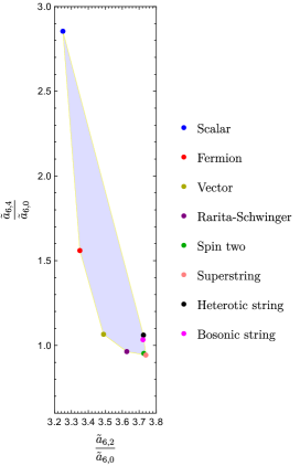
Figure 14: The transverse view of the theory island from Fig. 12. We indicate various theories that form the vertices of the island. To reach a particular point inside the UV island we need to take a superposition of various amplitudes.

A similar analysis can be performed for $k=8$. By switching to the $({\tilde{a}_{8,2}\over\tilde{a}_{8,0}},{\tilde{a}_{8,4}\over\tilde{a}_{8,0}},{\tilde{a}_{8,6}\over\tilde{a}_{8,0}})$ coordinates we note that the line from Fig. 13 maps to a single point. The same point can be obtained by keeping only $J=4$ contribution in (179)

$$\text{LSD}_{\alpha\to\infty}:~{}~{}~{}({\tilde{a}_{8,2}\over\tilde{a}_{8,0}},{\tilde{a}_{8,4}\over\tilde{a}_{8,0}},{\tilde{a}_{8,6}\over\tilde{a}_{8,0}})=(7,{35\over 8},{7\over 16})=(7,4.375,0.4375)\,.$$ (182)

Therefore by plotting the data in these coordinates we can resolve the points close to the origin in Fig. 13 which were located there due to the fact that $a_{8,0}\gg a_{8,i>0}$. One can check again that $({\tilde{a}_{8,2}\over\tilde{a}_{8,0}},{\tilde{a}_{8,4}\over\tilde{a}_{8,0}},{\tilde{a}_{8,6}\over\tilde{a}_{8,0}})$ is independent of $a_{8,0}$ and therefore this suppression does not take place anymore. The result is depicted in Fig. 15.

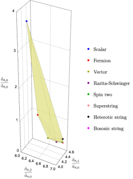
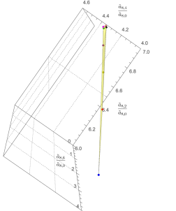
(a)	(b)

Figure 15: Various data points for $({\tilde{a}_{8,2}\over\tilde{a}_{8,0}},{\tilde{a}_{8,4}\over\tilde{a}_{8,0}},{\tilde{a}_{8,6}\over\tilde{a}_{8,0}})$. Panels a) and b) present the same plot as seen from different vantage points. In particular, panel b) makes it clear that the points essentially lie on a plane.

V.4 Spectral densities and low-spin dominance

In the discussion above we considered various bounds that follow from the dispersive representation of the low-energy couplings and observed the phenomenon of LSD in the known physical theories. It manifests itself in the fact that the low-energy couplings occupy a very small region in the space of couplings allowed on general grounds. To see this phenomenon more clearly it is instructive to look at the spectral densities of the amplitudes directly.

Given a known expression for the amplitude it is not hard to compute various spectral densities. Indeed, it amounts to taking a discontinuity of the amplitude and integrating it against the proper Wigner d-function. These satisfy a familiar orthogonality relation

$$\int_{-1}^{1}dx\,d_{\lambda,\lambda^{\prime}}^{J}(x)d_{\lambda,\lambda^{\prime}}^{\tilde{J}}(x)={2\over 2J+1}\delta_{J,\tilde{J}}\,.$$ (183)

For tree-level amplitudes the spectral density is a sum of delta-functions which correspond to the masses of exchanged particles. For the one-loop amplitudes the discontinuity has a continuous support above the two-particle threshold $4m^{2}$. In this case we perform the integration (183) numerically. We focus on the first few spin spectral densities in both $\rho_{J}^{++}$ and $\rho_{J}^{+-}$ channels. To go from spectral densities to the coefficients in the low-energy expansion we need to compute the moments as in Eqs. (165), (171), and (175).

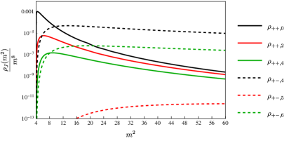
Figure 16: Spectral densities for the one-loop minimally-coupled scalar. We observe that $\rho_{0}^{++}\gg\rho_{J\geq 4}^{+-},\rho_{J\geq 2}^{++}$ and that $\rho_{4}^{+-}\sim\rho_{2}^{++}$ close to the two-particle threshold. This is fully consistent with the features of the plots for various couplings in the previous section.

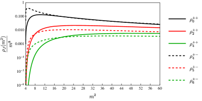
Figure 17: Spectral densities for the one-loop minimally coupled spin-2 particle. We observe that $\rho_{4}^{+-}\gg\rho_{J>4}^{+-},\rho_{J\geq 2}^{++}$ and that $\rho_{4}^{+-}\sim\rho_{0}^{++}$. Therefore in the space of couplings this amplitude is expected to lie on the low-spin dominance line.

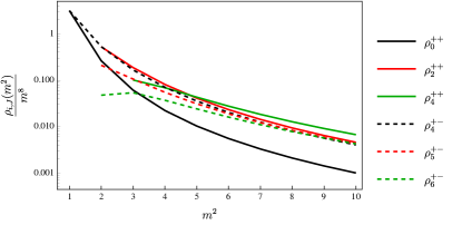
Figure 18: Spectral densities for the tree-level scattering of gravitons in the superstring theory. We observe that $\rho_{4}^{+-}\gg\rho_{J>4}^{+-},\rho_{J\geq 2}^{++}$ and that $\rho_{4}^{+-}\sim\rho_{0}^{++}$. Therefore in the space of couplings this amplitude is expected to lie on the low-spin dominance line.

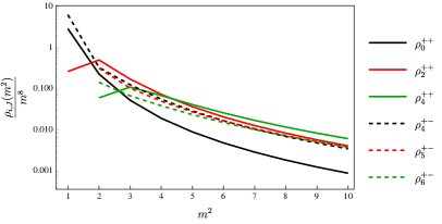
Figure 19: Spectral densities for the tree-level scattering of gravitons in the heterotic string theory. We observe that $\rho_{4}^{+-}\gg\rho_{J>4}^{+-},\rho_{J\geq 2}^{++}$ and that $\rho_{4}^{+-}\sim\rho_{0}^{++}$. Therefore in the space of couplings this amplitude is expected to lie on the LSD line.

The results for a few selected cased are listed in Fig. 16-19. In all cases we see that the minimal-spin partial waves dominate in the corresponding channel. It is also instructive to plot the moments $\langle\rho_{J}\rangle_{k}$ which we present in Fig. 20. The moments clearly satisfy LSD used in the previous section to derive stronger bounds.

Scalar loop	Spin 2 loop
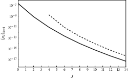
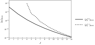
Superstring	Heterotic

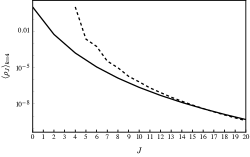
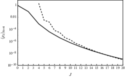
Figure 20: Moments of the spectral density $\langle\rho_{J}\rangle_{4}$ (148) as a function of spin $J$ for various examples. For the scalar one loop result $\rho_{J}^{+-}$ with $J$ being odd are negligible and are not presented in the figure. The line in the corresponding panel is obtained by connecting the even spin values of the spectral density moments.

In fact the moments of spectral density $\langle\rho_{J}\rangle_{k}$ in the examples we consider not only exhibit the dominance of the lowest-spin partial waves but also rapid decay at higher $J$. This latter feature is expected to be completely general. Indeed, the convergence of the sum rules (134) requires that $\langle\rho_{J}\rangle_{k}$ decay faster than any polynomial at large $J$. This latter decay can be traced to locality of scattering in the impact-parameter space.

Indeed, in the perturbative regime at large $J$ we have

$$\rho_{J}(s)\sim{\rm Im}\,\delta(s,b),~{}~{}~{}~{}~{}b={2J\over\sqrt{s}}\,,$$ (184)

where $\delta(s,b)$ is the phase shift and $b$ is the impact parameter. For fixed $s$ and large impact parameters we expect to have

$${\rm Im}\delta(s,b)\sim e^{-m_{\rm gap}b},~{}~{}~{}~{}~{}m_{\rm gap}b\gg 1\,,$$ (185)

which controls decay of $\rho_{J}(s)$ at large $J$. In string theory the leading-order behavior is different and is controlled by the transverse spreading of strings ${\rm Im}\,\delta(s,b)\sim e^{-{b^{2}\over 2\alpha^{\prime}\log{s\alpha^{\prime}\over 4}}}$—see Ref. Brower:2006ea .

A priori the large impact parameter discussion is not necessarily relevant for understanding the large-$J$ behavior of $\langle\rho_{J}\rangle_{k}$ which involves computing the moment (148) over all energies (as opposed to keeping $s$ fixed as we take the large-$J$ limit). However, in analyzing $\langle\rho_{J}\rangle_{k}$ for the amplitudes considered in the present paper we experimentally observed that the integral over energies is peaked at energies

$$\langle\rho_{J}\rangle_{k}:~{}~{}~{}{s_{*}\over m_{\rm gap}^{2}}\sim J.$$ (186)

Plugging this into the formula for the impact parameter (184) we find that the dominant impact parameters are $m_{\rm gap}b_{*}\sim J^{1/2}\gg 1$ and therefore the large-$J$ behavior of the moments $\langle\rho_{J}\rangle$ is still controlled by large impact-parameter physics. We tested this picture against the data presented in Fig. 20 and found a qualitative agreement. It would be interesting to study the large-$J$ limit of $\langle\rho_{J}\rangle_{k}$ more systematically. Of course, this discussion does not explain the fact that the hierarchical structure among partial waves continues all the way to the lowest spins in the examples we analyzed. It is this latter fact was crucial for the analysis in the previous section.

An important question is to understand how general is the picture that we observed in the tree-level string amplitudes and one-loop matter amplitudes. A priori these amplitudes look very different from each other, but at the level of the partial-wave analysis discussed in this section they exhibit remarkably similar behavior and strong version of LSD. This suggests that the hierarchical structures we observed in this paper could be a general property of consistent weakly-coupled gravitational $S$-matrices, but we do not have a proof yet.

V.5 A hierarchy from unitarity

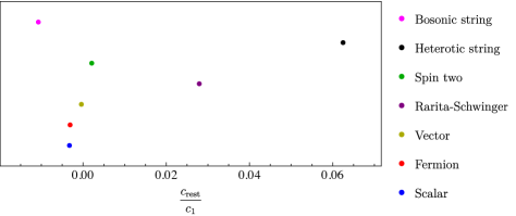
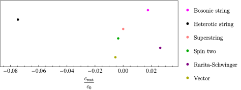
Figure 21: Examples of a hierarchy from unitarity. The horizontal axis shows illustrates that the dominance of low-spin spectral densities naturally introduces a $10^{-2}$ hierarchy between various EFT coefficients in the absence of any symmetry. The vertical axis carries no meaning other than separating the points.

The LSD discussion above illustrates an interesting phenomenon of emergent hierarchy between EFT coefficients in the absence of an underlying symmetry. Consider for example $D^{8}R^{4}$ type corrections discussed in the $k=4$ section above. In writing down the relevant correction to the amplitude an EFT practitioner guided by the considerations of the supersymmetric decomposition (32) can write the following ansatz

$$f_{D^{8}R^{4}}(t,u)=c_{0}\,(s^{2}+t^{2}+u^{2})^{2}+c_{1}\,s^{4}+c_{\rm{rest}}\,(t^{2}+u^{2})^{2}\,.$$ (187)

The first term, which is proportional to $c_{0}$, is the completely crossing-symmetric term of the type that appears in the new spin-2 part of the amplitude given in Eq. (302), corresponding to a massive ${\mathcal{N}}=8$ supersymmetric multiplet, obtained, for example, by dimensional reduction from five dimensions. In the ${\mathcal{N}}=8$ theory the full crossing symmetry of such terms is a consequence of $\mathcal{N}=8$ supersymmetric Ward identities SWI . The $c_{1}$ term corresponds to the additional terms needed in the new spin-3/2 part of the amplitude (301) beyond the fully crossing symmetric terms already appearing in the new spin-2 part of the amplitude. Finally, the third term containing $c_{\text{rest}}$ is the remaining independent term with $t$–$u$ crossing symmetry. This term is distinguished from the $c_{1}$ term by its differing behavior for $t\rightarrow\infty$ with $s$ fixed.

We then express the coefficient above in terms of more familiar $a_{k,j}$ defined in Eq. (131) and used in the discussion of various bounds. We get the following result

$$c_{0} ={1\over 4}(2a_{4,1}-a_{4,2})\,,$$

$$c_{1} ={1\over 4}(4a_{4,0}-5a_{4,1}+2a_{4,2})\,,$$

$$c_{\text{rest}} ={1\over 2}(a_{4,2}-{3\over 2}a_{4,1})\,.$$ (188)

Remarkably, we see that $c_{\text{rest}}$ vanishes along the low-spin dominance line that follows from Eq. (165). Plugging in the values of $a_{k,j}$ for the theories discussed here we find a $10^{-2}$ hierarchy with $c_{\text{rest}}\ll c_{1}$ in the absence of any symmetry, as shown in Fig. 21. For spin $S=1,{3\over 2},2$ particle in the loop we also have $c_{\text{rest}}\ll c_{0}$.

VI Deriving bounds: multiple polarizations

In this section we consider dispersion relations that combine information from the different helicity configurations. More precisely, we consider dispersive sum rules (121) which we apply to the matrices built out of various scattering amplitudes (110), (111). We derive bounds on the inelastic amplitudes (single-minus and all-plus amplitudes) in terms of the elastic double-minus amplitude.

VI.1 $s=0$

The simplest bounds comes from setting $s=0$ in Eq. (122). The relevant equation takes the form

$$\oint_{t_{0}}{dt\over 2\pi i}\mathcal{M}_{h}(s,t){1\over t}{1\over(t(s+t))^{k}}\Big{|}_{s=0}=\int_{m_{\rm gap}^{2}}^{\infty}{dt\over\pi}{2\over t^{2k+1}}{\rm Disc}_{t}\mathcal{M}_{h}(0,t)\succeq 0\,.$$ (189)

By plugging the low-energy expansion of the amplitude in the LHS of the equation above and requiring that its eigenvalues are non-negative we get

$$2f_{2k-4,0}\geq|h_{2k,0}|\,,~{}~{}~{}~{}k=2,4,6,\ldots\,.$$ (190)

The combination above for different $k$ form a set of moments as can be seen from the RHS of (189). The difference compared to the recent analysis in Ref. Bellazzini:2020cot is that in our case we have a positive semi-definite spectral density matrix instead of a function. By contracting such matrix moments with an arbitrary polarization vector reduces the problem to the one considered in Ref. Bellazzini:2020cot .

The situation simplifies in the parity preserving case when $h^{*}(s,u)=h(s,u)$. In this case the eigenvectors $\mathcal{M}_{h,\pm}(s,t)$ given in Eq. (IV.2) generate the low-energy expansion that satisfies the moment problem conditions considered in great detail in Ref. Bellazzini:2020cot . More precisely, we define a set of moments as $\mu_{{k-1}}\equiv 2f_{2k-4,0}-h_{2k,0}$ and consider the Hankel matrix $H_{ij}=\mu_{i+j-1}$.

Using the results in Appendix H for the one-loop amplitude due to minimally-coupled scalar in the loop the first five moments take the following form

$$H^{S=0}={1\over 140}\left(\frac{\kappa}{2}\right)^{4}{1\over(4\pi)^{2}}\left(\begin{array}[]{ccc}\frac{1}{135m^{4}}&\frac{1}{24024m^{8}}&\frac{1}{1969110m^{12}}\\ \frac{1}{24024m^{8}}&\frac{1}{1969110m^{12}}&\frac{1}{109745064m^{16}}\\ \frac{1}{1969110m^{12}}&\frac{1}{109745064m^{16}}&\frac{1}{4833678850m^{20}}\\ \end{array}\right).$$ (194)

In agreement with the general prediction the one-loop moment matrix has nonnegative minors.

VI.2 Away from $s=0$: first derivative

We can use (113) to derive the bounds by taking the derivative of $B^{+}_{k}(s)$ with respect to $s$ before setting $s=0$. For example let us consider the first derivative with respect to $s$. In this way we get

$$\partial_{s}\oint_{t_{0}}{dt\over 2\pi i} \mathcal{M}_{h,g}(s,t){1\over t}{1\over(t(s+t))^{k}}\Bigr{|}_{s=0}$$

$$=\int_{m_{\rm gap}^{2}}^{\infty}{dt\over\pi}{1\over t^{2k+2}}\left(-(2k+1){\rm Disc}_{t}\mathcal{M}_{h,g}(0,t)+2t\,\partial_{s}{\rm Disc}_{t}\mathcal{M}_{h,g}(0,t)\right).$$ (195)

The RHS is not positive semi-definite and therefore we cannot derive the bound on the LHS in a similar fashion. We can, however, consider the following linear combination

$${2k+1\over 2m_{\rm gap}^{2}}\oint_{t_{0}}{dt\over 2\pi i}\mathcal{M}_{h,g}(s,t){1\over t}{1\over(t(s+t))^{k}}+\partial_{s}\oint_{t_{0}}{dt\over 2\pi i}\mathcal{M}_{h,g}(s,t){1\over t}{1\over(t(s+t))^{k}}\Big{|}_{s=0}$$

$$\hskip 8.5359pt=\int_{m_{\rm gap}^{2}}^{\infty}{dt\over\pi}{1\over t^{2k+2}}\left(\Bigl{[}{t\over m_{\rm gap}^{2}}-1\Bigr{]}(2k+1){\rm Disc}_{t}\mathcal{M}_{h,g}(0,t)+2t\,\partial_{s}{\rm Disc}_{t}\mathcal{M}_{h,g}(0,t)\right)\succeq 0\,.$$ (196)

We now apply Eq. (VI.2) to $\mathcal{M}_{h}$. By plugging the low-energy expansion (see Eqs. (98) and (68)) in the LHS of the formula above and imposing that the eigenvalues of the resulting matrix are nonnegative we can derive various bounds. Let us consider for example $k=2$. We get the following bound on the inelastic amplitude in terms of the elastic one

$$\boxed{\Big{|}h_{5,1}+{5\over 2}{h_{4,0}\over m_{\rm gap}^{2}}\Big{|}\leq 5\Bigl{(}f_{1,0}+{f_{0,0}\over m_{\rm gap}^{2}}\Bigr{)}-2|\beta_{R^{3}}|^{2}\,.}$$ (197)

To apply the dispersive sum rule above to the bosonic string amplitude we first subtracted the contribution of the tachyon exchange to get $\delta f^{(\text{bs})}(s,u)=f^{(\text{bs})}(s,u)+\left(\frac{\kappa}{2}\right)^{2}{1\over 1+t}$ and $\delta\,h^{(\text{bs})}(s,u)=h^{(\text{bs})}(s,u)+\left(\frac{\kappa}{2}\right)^{2}\left({s^{4}\over 1+s}+{t^{4}\over 1+t}+{u^{4}\over 1+u}\right)$. The resulting functions satisfy all the properties needed to apply (VI.2) for $k=2$. We then get, using the formulas from App. B,

$$\delta f^{(\text{bs})}_{0,0} =\left(\frac{\kappa\hbox{}}{2}\right)^{2}\Big{(}3+2\zeta(3)\Big{)},~{}~{}~{}~{}~{}\delta f^{(\text{bs})}_{1,0}=\left(\frac{\kappa\hbox{}}{2}\right)^{2}(-3),$$

$$\delta\,h^{(\text{bs})}_{4,0} =\left(\frac{\kappa\hbox{}}{2}\right)^{2}2,~{}~{}~{}~{}~{}\delta h^{(\text{bs})}_{5,1}=\left(\frac{\kappa\hbox{}}{2}\right)^{2}(-3),~{}~{}~{}|\beta_{R^{3}}^{(\text{bs})}|^{2}=\left(\frac{\kappa\hbox{}}{2}\right)^{2}.$$ (198)

which indeed satisfy Eq. (197) where $m_{\rm gap}^{2}=1$ in the string case.

For the one-loop minimally coupled scalar $|\beta_{R^{3}}|^{2}\sim\kappa^{6}$ and appears only at two loops. For other coefficients that enter into Eq. (197) we get, using Eq. (86) and Eq. (91),

$$f_{0,0}^{S=0} =\left(\frac{\kappa}{2}\right)^{4}{1\over(4\pi)^{2}}{1\over 6300m^{4}},~{}~{}~{}f_{1,0}^{S=0}=-\left(\frac{\kappa}{2}\right)^{4}{1\over(4\pi)^{2}}{1\over 41580m^{6}}\,,$$

$$h_{4,0}^{S=0} =\left(\frac{\kappa}{2}\right)^{4}{1\over(4\pi)^{2}}{1\over 3780m^{4}},~{}~{}~{}h_{5,1}^{S=0}=-\left(\frac{\kappa}{2}\right)^{4}{1\over(4\pi)^{2}}{1\over 7920m^{6}}\,,$$ (199)

so that, together with $m_{\rm gap}^{2}=4m^{2}$, (197) is again satisfied.

More generally, the formula above bounds the correction to the three-point function of the graviton $\beta_{R^{3}}$ from above in terms of the EFT data. To make it more manifest we can rewrite the above

$$2|\beta_{R^{3}}|^{2}\leq 5\Bigl{(}f_{1,0}+{f_{0,0}\over m_{\rm gap}^{2}}\Bigr{)}-\Big{|}h_{5,1}+{5\over 2}{h_{4,0}\over m_{\rm gap}^{2}}\Big{|}\leq{10f_{0,0}\over m_{\rm gap}^{2}}\,,$$ (200)

where in the last inequality we used the fact that $|f_{1,0}|\leq{1\over m_{\rm gap}^{2}}f_{0,0}$ which readily follows from Eqs. (132) and (134). We can restate it more succinctly in terms of the Wilson coefficients of the gravitational EFT

$$|\beta_{R^{3}}|^{2}\leq 5{\beta_{R^{4}}^{+}\over m_{\rm gap}^{2}}\,,$$ (201)

where $m_{\rm gap}^{2}$ denotes the mass gap at which the massive degrees of freedom that induce the higher-derivative corrections appear. Recall that $f_{0,0}=\beta_{R^{4}}^{+}$ was defined in Eq. (84). Bounds similar to Eq. (200) can be derived by considering the superconvergence sum rules for $k>2$. We do not list them here.

In fact it is not difficult to strengthen the bound (201) by considering the following unsubtracted dispersive sum rule (analogous to $k=0$ in Eq. (121))

$$\oint_{\infty}{dt\over 2\pi i}{1\over t}f(s,-s-t)=0\,.$$ (202)

The universal tree-level gravitational piece $\left({\kappa\over 2}\right)^{2}{1\over stu}$, which is singular at $s=0$, does not contribute to Eq. (202) therefore we can consider

$$\left({1\over m_{\rm gap}^{2}}+\partial_{s}\right)\eqref{eq:relationB0}\Big{|}_{s=0}:~{}~{}~{}~{}{\beta_{R^{4}}^{+}\over m_{\rm gap}^{2}}-|\beta_{R^{3}}|^{2}=$$

$$\hskip 71.13188pt\int_{m_{\rm gap}^{2}}^{\infty}{dt\over\pi}{1\over t}\left(\Bigl{[}\partial_{s}+{1\over m_{\rm gap}^{2}}\Bigr{]}{\rm Disc}_{t}f+\Bigl{[}\partial_{s}+{t-m_{\rm gap}^{2}\over m_{\rm gap}^{2}t}\Bigr{]}{\rm Disc}_{u}f\right)\Big{|}_{s=0}\geq 0\,,$$ (203)

where nonnegativity of the RHS can be readily checked for each partial wave separately by plugging the discontinuities of $f(s,u)$, given in Eq. (133), into the formula above. In this way we immediately get a bound

$$\boxed{|\beta_{R^{3}}|^{2}\leq{\beta_{R^{4}}^{+}\over m_{\rm gap}^{2}}\,.}$$ (204)

The bound (204) is a step towards making the analysis of Ref. Camanho:2014apa quantitatively precise. At least for the $R^{3}$ correction to the graviton three-point coupling which is considered here, it translates the problem to bounding the coefficient $\beta_{R^{4}}^{+}$ in terms of $G/m_{\rm gap}^{2}$. This problem was beautifully solved recently in Ref. Caron-Huot:2021rmr for $D=10$ maximal supergravity in a perturbative setting similar to ours, and it was addressed nonperturbatively in Ref. Guerrieri:2021ivu . The method used in Ref. Caron-Huot:2021rmr is not directly applicable in four dimensions due to the IR divergences, but at least in $D\geq 5$ where the $2\to 2$ amplitude is nonperturbatively well-defined it is natural to expect that one will be able to get a bound on $\beta_{R^{4}}^{+}$ in terms of ${G/m_{\rm gap}^{2}}$. It would be very interesting to demonstrate it explicitly.

Indeed, assuming the nonperturbative Regge bound (119), we can consider the $(-2)$ subtracted dispersion relations for $f(s,u)$ which expresses $-{8\pi G/s}$ in terms of the contribution of heavy states, cf. equation (3.37) in Ref. Caron-Huot:2021rmr . Existence of such a dispersion relation in the absence of supersymmetry is crucially due to the fact that we consider gravitons as external states.

VI.3 Away from $s=0$: second derivative

Using exactly the same technique as above one can check that

$${2k^{2}-1\over 4}\oint_{t_{0}}{dt\over 2\pi i}\mathcal{M}_{h,g}(s,t){1\over t}{1\over(t(s+t))^{k}}+{2k+1\over 2t_{0}}\partial_{s}\oint_{t_{0}}{dt\over 2\pi i}\mathcal{M}_{h,g}(s,t){1\over t}{1\over(t(s+t))^{k}}$$

$$\hskip 85.35826pt+\partial_{s}^{2}\oint_{t_{0}}{dt\over 2\pi i}\mathcal{M}_{h,g}(s,t){1\over t}{1\over(t(s+t))^{k}}\Big{|}_{s=0}\succeq 0\,.$$ (205)

Consider $k=2$ and plug the low-energy expansion of $\mathcal{M}_{g}(s,t)$ in the formula above. We get a matrix whose eigenvalues should be non-negative. In this way we can bound the constant term in the $++-+$ amplitude

$$\boxed{|g_{0,0}|\leq{7\over 4}{f_{0,0}\over(m_{\rm gap}^{2})^{2}}+{5\over 4}{5f_{1,0}-4|\beta_{R^{3}}|^{2}\over m_{\rm gap}^{2}}+{3\over 2}\left(f_{2,0}+3f_{2,1}\right)\,.}$$ (206)

As in the previous section we can check (206) in the bosonic string theory. The extra data compared to the previous section takes the form

$$g_{0,0}^{(\text{bs})} =\left(\frac{\kappa\hbox{}}{2}\right)^{2}\Big{(}2\zeta_{3}\Big{)},~{}~{}~{}\delta f_{2,0}^{(\text{bs})}=\left(\frac{\kappa\hbox{}}{2}\right)^{2}\Big{(}3+2\zeta(5)\Big{)},$$

$$\delta f_{2,1}^{(\text{bs})} =\left(\frac{\kappa\hbox{}}{2}\right)^{2}\Big{(}2+4\zeta(3)+2\zeta(5)\Big{)}.$$ (207)

Plugging (VI.3) into Eq. (206) we see that it is indeed satisfied.

For the one-loop minimally coupled scalar we get correspondingly

$$g_{0,0}^{S=0} =\left(\frac{\kappa}{2}\right)^{4}{1\over(4\pi)^{2}}{1\over 6306300m^{8}}\,,~{}~{}~{}~{}~{}f_{2,0}^{S=0}=\left(\frac{\kappa}{2}\right)^{4}{1\over(4\pi)^{2}}{3\over 560560m^{8}},$$

$$f_{2,1}^{S=0} =\left(\frac{\kappa}{2}\right)^{4}{1\over(4\pi)^{2}}{31\over 9081072m^{8}}\,.$$ (208)

Again, we checked that Eq. (206) is satisfied, where we set $m_{\rm gap}^{2}=4m^{2}$.

Using the bounds from the previous section and (206) we can bound $g_{0,0}$ in terms of $\beta^{+}_{R^{4}}$ defined in Eq. (66) as follows

$$|g_{0,0}|\leq{815\over 44}{\beta^{+}_{R^{4}}\over m_{\rm gap}^{4}}\,.$$ (209)

In deriving (209) we first expressed $f_{i,j}$, defined in Eq. (98), in terms of $a_{k,j}$, defined in Eq. (131), and then used Eqs. (138) and (146). Assuming LSD we get a stronger bound

$$\text{LSD}_{\alpha\to\infty}:~{}~{}~{}~{}~{}|g_{0,0}|\leq{25\over 4}{\beta^{+}_{R^{4}}\over m_{\rm gap}^{4}}\,,$$ (210)

where in deriving this we used the stronger LSD bound (154).

VII Conclusions

Our paper naturally consisted of two parts with the first part providing theoretical data that we interpreted in the second part in terms of bounds on coefficients of gravitational EFTs. In the first part, using amplitudes methods, we obtained the one-loop four-graviton amplitude with a minimally-coupled massive particle of spin up to $S=2$ circulating in the loop. By series expanding these amplitude in large mass, we obtain theoretical data for Wilson coefficients which we analyze in the second part. Combining this data with similar theoretical data obtained from tree-level string-theory amplitudes we found that the Wilson coefficients fall on small islands compared to the general bounds coming from consistency of $2\to 2$ scattering determined along the lines of Refs. Tolley:2020gtv ; Caron-Huot:2020cmc ; Arkani-Hamed:2020blm . It is quite striking that the EFT coefficients derived from both string-theory and one-loop-massive amplitudes land on the same small islands. Remarkably this can be explained as a consequence of low-spin dominance in the partial-wave expansions.

VII.1 Obtaining one-loop amplitudes

In order to compute the one-loop amplitudes used to generate EFT data we applied standard amplitudes methods, including spinor helicity SpinorHelicity , generalized unitarity Unitarity ; BernMorgan , the double copy Kawai:1985xq ; BCJ ; BCJReview and integration by parts IBP ; Smirnov:2019qkx . Using generalized unitarity we obtained all integral coefficients except for a few whose integrals have no unitarity cuts in any channel. We fixed the coefficients of the latter integrals by using the known ultraviolet properties of the amplitude. To fully utilize this information we made use of overcomplete integral basis that contains higher-dimensional integrals, but whose coefficients do not depend on the spacetime dimension or equivalently the dimensional-regularization parameter $\epsilon$. In addition, we also demonstrated that these coefficients do not depend on the mass $m$ of the particles circulating in the loops. The existence of such a basis imposes constraints that makes it reasonably straightforward to determine any pieces not captured by the $s$, $t$ and $u$ channel unitarity cuts. In this basis we used the fact that the coefficient of the potential $1/\epsilon$ logarithmic ultraviolet divergence is zero tHooft:1972tcz to completely fix the remaining integral coefficients. A basis without $\epsilon$-dependent coefficients always exists for one-loop problems Bern:1995ix , however the lack of $m$-dependence appears to be special to our case of a closed massive loop with external massless particles.

It would of course be interesting whether there is some way to generalize our approach to more complicated situations with external legs of differing masses. To generalize our approach to the generic case of a massive one-loop amplitude one could use information from the higher-than-logarithmic divergences which are accessible in dimensional regularization by shifting the dimension downwards as discussed in Sect. II.5. We showed that knowledge of all these divergences is sufficient to fully constrain the remaining ambiguities, something we expect to be true more generally. We expect constraints from ultraviolet divergences and from requiring proper decoupling in the large mass limit to be sufficient to remove any ambiguities in terms that are not fixed by the unitarity cuts, up to the usual ambiguities tied to scheme choices and renormalization. This may provide an alternative method for obtaining complete one-loop amplitudes using on-shell techniques BrittoMirabella .

We exposed a useful supersymmetric decomposition for graviton amplitudes with a massive particle in the loop. A similar decomposition exists in gauge theory Bern:1993tz . This decomposition expressed the amplitude with a particle of spin $S$ in the loop in terms of amplitudes with lower-spin particles and simpler to calculate pieces. These pieces correspond to amplitudes with a massive BPS multiplet circulating in the loop.

Having constructed the one-loop four-graviton amplitudes with massive particles in the loop, it was then straightforward to expand in large mass, generating amplitudes matching those from a gravitational EFT. Because the original amplitudes are sensible, satisfying appropriate Regge behavior and unitarity, this EFT is also sensible and can be used to test the constraints derived from dispersion relations.

Besides using these results in our study of bounds on EFT coefficients, we also noted a simple relations between ultraviolet divergences in higher dimensions and the coefficients in the $1/m$ expansion. This relation requires a particular analytic continuation of the amplitude to higher dimensions where we keep the number of physical states at their four-dimensional values. It would be interesting to see if similar relations hold more generally, including higher loops, and whether this connection can be exploited in studies of bounds on EFT coefficients.

VII.2 EFT bounds

In order to derive bounds on the Wilson coefficients, we first reviewed in Sect. IV the basic properties of unitarity, crossing, and bounds on the Regge limit in the context of perturbative $2\to 2$ scattering of gravitons in four dimensions. These allowed us to study dispersion relations and derive bounds on the Wilson coefficients.

In Sect. V we focused on the double-minus amplitude and derived bounds on the Wilson coefficients along the lines of Ref. Tolley:2020gtv ; Caron-Huot:2020cmc ; Arkani-Hamed:2020blm . We expressed the low-energy expansion coefficients as dispersive integrals in Eq. (134). We then identified the two-sided bounds on the coefficients following the observation in Ref. Arkani-Hamed:2020blm that the boundaries of the allowed region inherit the cyclicity property from the one channel dispersion relation. In this way, by explicitly extracting the mixed constraints from the mixed $s$–$u$ channel partial waves we identified the new boundaries of the allowed region. We do not rigorously prove that our identification of the bounds is optimal, and we leave filling this gap for future work. We then introduced the idea of LSD which expresses a relationship between moments of the spectral functions of various spins, and we used crossing symmetry or null constraints Caron-Huot:2020cmc to derive rigorous bounds in terms of a few low-spin partial waves. We found that all the amplitudes considered in this paper lie on small islands whose location and shape can be determined using the low-spin dominance principle.

In Sect. VI we studied dispersion relations for the graviton amplitudes of various helicities. The key observation is that we can apply dispersion relations to matrices (102), composed of the different helicity amplitudes, whose discontinuity is positive semi-definite. Applying dispersive sum rules along the lines of Ref. Caron-Huot:2020cmc to these matrices we derived constraints on the Wilson coefficients which appear in the single-minus and all-plus gravitational scattering amplitudes. Notably we placed a bound on the $R^{3}$ coefficient that corrects the graviton three-point amplitude in terms of the $R^{4}$ coefficient, making a step towards making the analysis of Ref. Camanho:2014apa quantitatively precise.

The idea that the set of possibilities to UV complete gravity is much sparser than one naively would have thought lies at the heart of the swampland program swampland . Usually this sparseness is associated with non-perturbative aspects of the UV completion. In the present paper we analyzed the problem in a perturbative setting. By minimally coupling low-spin matter to gravity we generated $S$-matrices which we expect should satisfy the axioms of causality and unitarity up to an arbitrary order in $G$ and in an arbitrary $n$-point amplitude. We can ask therefore a weaker version of the swampland question: what is the set of perturbatively consistent weakly-coupled gravitational $S$-matrices? It is in the framework of this question that the analysis of the present work can be placed. Unexpectedly, we found that in known examples of perturbatively consistent gravitational $S$-matrices the low-energy couplings lie in regions much smaller than predicted on general grounds of causality and positivity of $2\to 2$ graviton scattering. Looking at the amplitudes for tree-level string theory and minimally coupled one-loop matter it is not a priori obvious at all that they should be “close” to each other. Dispersive representation of the low-energy expansion of both makes this similarity apparent. Indeed, as discussed in Sect. V both amplitudes satisfy strong versions of LSD that localizes their low-energy data to regions that are much smaller than indicated by the general analysis of unitarity and crossing.

An obvious question is: how general is this universality? We motivated it by pointing out that the examples considered in the present paper define consistent $S$-matrices for any $n\to m$ scattering, whereas the bounds were derived by considering $2\to 2$ scattering only. To answer this question we would need to better understand the landscape of consistent gravitational amplitudes, including any unitary perturbative or nonperturbative QFT coupled to gravity, as well as amplitudes in theories with extra dimensions. In particular, it would be very interesting to understand if and how consistency of $n\to m$ scattering can be used to rigorously establish stronger bounds on $2\to 2$ scattering, potentially bringing us closer to the small theory islands observed in the present work. It would also be very interesting to understand the example of large-$N$ QCD coupled to gravity Kaplan:2020tdz .

In this paper, we only considered the leading-order effect from integrating out massive degrees of freedom. We did not address the question of bounds that can be applied to IR-safe observables in four dimensions, nor have we included the loops of massless particles which generate more general logarithmic corrections in the low-energy expansion of the amplitude. We leave these important questions to future work. The logarithmic running was discussed in Refs. Bellazzini:2020cot ; Trott:2020ebl ; Arkani-Hamed:2020blm , with the basic idea being that instead of expanding the amplitude around $s,t=0$ one considers dispersive representations of the EFT couplings defined at some scale. To deal with the IR divergences we may consider dressed states (see e.g. Ref. Strominger:2017zoo ; Arkani-Hamed:2020gyp for a recent discussion), for which the full implications of unitarity and crossing are still to be fully understood. Another interesting problem is to repeat the analysis of the present paper in the context of $\rm AdS_{4}/CFT_{3}$ where the problem of IR divergences does not arise, but dispersive techniques discussed in the present paper still hold CFTdispersion .

In summary, motivated by low-energy theoretical data obtained from one-loop field-theory and tree-level string-theory amplitudes, we put forward the idea that EFTs that describe sensible weak gravitational theories live on small islands that can be understood in terms of partial-wave low-spin dominance. It will be important to understand the extent to which this can be extended to constrain gravitational theories.

Acknowledgements:

We are grateful to Nima Arkani-Hamed, Thomas Dumitrescu, Kelian Häring, Enrico Hermann, Tzu-Chen Huang, Yu-tin Huang, Julio Para-Martinez, Marco Meineri, Irina Mocioiu, Baur Mukhametzhanov, Radu Roiban, Eric Sawyer, Chia-Hsien Shen, and Piotr Tourkine for helpful conversations. This work was supported by the U.S. Department of Energy (DOE) under award number DE-SC0009937. This project has received funding from the European Research Council (ERC) under the European Union’s Horizon 2020 research and innovation programme (grant agreement number 949077). D. K. also thanks the Mani L. Bhaumik Institute for Theoretical Physics for support.

Appendix A Minimal Coupling

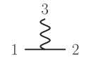
Figure 22: The three-point amplitude necessary to study minimal coupling. The straight lines represent massive spinning particles, while the wiggly line denotes either a photon or a graviton.

In this appendix we present in more detail our definition of minimal coupling of gravity to a massive spinning particle. For massive spinning particles, the requirement of general-coordinate invariance and mass-dimension-4 operators leaves an ambiguity for integer spin-particles in defining the minimal coupling to gravity. In this appendix we discuss this ambiguity and the choice we make in this paper. Our choice corresponds to the one that does not violate the unitarity and causality constraints of Refs. treeLevelUnitarity ; Bonifacio:2017nnt ; Afkhami-Jeddi:2018own ; Meltzer:2017rtf ; Afkhami-Jeddi:2018apj . We start by reviewing the case of electromagnetism (EM) where a similar situation exists, before we move on to consider the gravitational case.

This issue appears only for integer-spin particles. The source of the ambiguity is the existence of a gauge-invariant operator that has the same mass dimension as the kinetic term. For half-integer-spin particles, the corresponding operator is of higher-mass dimension and hence would not count as minimal coupling. Therefore, the cases that require attention are the coupling of a spin-1 or spin-2 particle to gravity. Since the analysis of the coupling of a spin-1 particle to EM is similar, we start by reviewing this case.

Here we fix the ambiguity by requiring that the interactions smoothly match onto the massless limit. To explain our choice, it suffices to evaluate the three-point amplitude between two massive spinning particles and a photon or a graviton. Specifically, we demand that by taking the massless limit of these amplitudes and identifying the spin-1 particles as gauge bosons and the spin-2 particles as gravitons, we recover the corresponding amplitudes in Yang-Mills and pure gravity. The former is indeed realized for the coupling of the W boson to the photon PeskinSchroeder . The double-copy construction used in this paper is smooth in the massless limit, and hence selects the above prescription.

For this discussion, we follow the formalism of Refs. Singh:1974qz , which allows us to discuss particles of arbitrary spin. After obtaining the relevant three-point amplitudes, we specialize to the cases of interest. The part of the Lagrangian we give is just the one necessary to obtain the three-point amplitudes relevant for this discussion. We emphasize that these Lagrangians would need to be modified with auxiliary-field terms in order to reproduce our one-loop calculation.

For the case of a massive spinning particle $\phi$ coupled to EM we have

$$\mathcal{L}=-\frac{1}{4}F_{\mu\nu}F^{\mu\nu}+D_{\mu}^{\dagger}\bar{\phi}D^{\mu}\phi-m^{2}\bar{\phi}\phi+e(g-1)F_{\mu\nu}\,\bar{\phi}M^{\mu\nu}\phi+\ldots\,,$$ (211)

where $e$ is the charge of the particle, $g$ is the gyromagnetic ratio and the ellipsis denote possible auxiliary-field terms. For the Lorentz generator $M$ in the representation of $\phi$ we may use

$$(M^{\mu\nu}){}_{c(s)}{}^{d(s)}={2{}i{}s}\delta^{[\mu}_{(c_{1}}\eta^{\nu](d_{1}}\delta^{d_{2}}_{c_{2}}\dots\delta^{d_{s})}_{c_{s})}\,,$$ (212)

where the indices $c(s)$ and $d(s)$ stand for the symmetrized sets of vector indices $\{c_{1},\dots,c_{s}\}$ and $\{d_{1},\dots,d_{s}\}$ and symmetrizations include division by the number of terms.

We may now obtain the three-point amplitude between two massive spinning particles and a photon, depicted in Fig. 22. Neglecting the overall normalization we find

$$\mathcal{A}^{\text{EM}-s}_{3}\sim\varepsilon_{1}\cdot\varepsilon_{2}\,\varepsilon_{3}\cdot p_{1}+i(g-1)\varepsilon_{1}\cdot M[\varepsilon_{3},p_{3}]\cdot\varepsilon_{2}\,,$$ (213)

where labels 1 and 2 denote the massive spinning particles, while particle 3 is a photon. We use the notation

$$A\cdot M[p,q]\cdot B\equiv p_{\mu}q_{\nu}(M^{\mu\nu}){}_{c(s)}{}^{d(s)}A^{c(s)}B_{d(s)}\,.$$ (214)

Plugging in the spin-1 representation for $M$ we find

$$\mathcal{A}^{\text{EM}-1}_{3}\sim\varepsilon_{1}\cdot\varepsilon_{2}\,\varepsilon_{3}\cdot p_{1}+(g-1)\Big{(}\varepsilon_{3}\cdot\varepsilon_{1}\,\varepsilon_{2}\cdot p_{3}-\varepsilon_{2}\cdot\varepsilon_{3}\,\varepsilon_{1}\cdot p_{3}\Big{)}\,.$$ (215)

Identifying all three particles as gauge bosons in the massless limit, i.e. demanding $\mathcal{A}^{\text{EM}-1}_{3}=\mathcal{A}^{\text{YM}}_{3}$, fixes $g=2$.

The case of a massive spinning particle coupled to gravity is similar. In this case, we have

$${\cal L} =-\frac{1}{16\pi G}R+\frac{1}{2}g^{\mu\nu}\nabla_{\mu}\phi\nabla_{\nu}\phi-\frac{1}{2}m^{2}\phi\phi+\frac{\rm H}{8}R_{\kappa\lambda\mu\nu}\,\phi M^{\kappa\lambda}M^{\mu\nu}\phi+\ldots\,,$$ (216)

where $\rm H$ is an arbitrary dimensionless coefficient and we again denote possible auxiliary-field terms by the ellipsis. Plugging in the spin-1 representation we see that the Riemann tensor in the term proportional to $\rm H$ contracts into the Ricci tensor or scalar which under the equations of motion is equivalent to a $\phi^{2}$ term. Therefore, the $\rm H$ term may be replaced by using an appropriate field redefinition by a $\phi^{4}$-type term, which is not relevant for our discussion. Looking at the spin-2 representation and taking the massless limit, we recover the background-field-gauge gravitational Lagrangian of Ref. Bern:1993wt for $\rm H=1$ upon identifying the spin-2 particle with the graviton.

We may alternatively reach the same conclusions by looking at the three-point amplitude between two massive spinning particles and a graviton. This amplitude, shown in Fig. 22, is given by

$$\mathcal{M}^{\text{GR}-s}_{3}\sim-\varepsilon_{1}\cdot\varepsilon_{2}(\varepsilon_{3}\cdot p_{1})^{2}+i(\varepsilon_{3}\cdot p_{1})\varepsilon_{1}\cdot M[\varepsilon_{3},p_{3}]\cdot\varepsilon_{2}+\frac{\rm H}{2}\varepsilon_{1}\cdot M[\varepsilon_{3},p_{3}]\cdot M[\varepsilon_{3},p_{3}]\cdot\varepsilon_{2}\,.$$ (217)

For the spin-1 representation of $M$ we observe that the last term vanishes. For the spin-2 representation we have

$$\mathcal{M}^{\text{GR}-2}_{3}\sim-\varepsilon_{1}\cdot\varepsilon_{2} (\varepsilon_{3}\cdot p_{1})^{2}-2\,\varepsilon_{1}^{\mu\kappa}\varepsilon_{2,\kappa}^{\nu}(\varepsilon_{3,\mu}p_{3,\nu}-\varepsilon_{3,\nu}p_{3,\mu})(\varepsilon_{3}\cdot p_{1})$$

$$-\text{H}\,\varepsilon_{1}^{\mu\nu}\varepsilon_{2}^{\alpha\beta}(\varepsilon_{3,\mu}p_{3,\nu}-\varepsilon_{3,\nu}p_{3,\mu})(\varepsilon_{3,\alpha}p_{3,\beta}-\varepsilon_{3,\beta}p_{3,\alpha})\,.$$ (218)

Identifying the spin-2 particles with gravitons, i.e. setting $\mathcal{M}^{\text{GR}-2}_{3}$ equal to the three-point amplitude in pure gravity, we find $\rm H=1$.

With this choice our one-loop amplitudes do not violate unitarity or causality constraints treeLevelUnitarity ; Meltzer:2017rtf ; Afkhami-Jeddi:2018apj ; Camanho:2014apa . Hence, they serve as toy models of causal UV completions.

Appendix B Tree-level string amplitudes

Here we collect the relevant string four-graviton tree-level amplitudes Kawai:1985xq

$$\mathcal{M}_{4}^{(\text{ss})}(1^{+},2^{-},3^{-},4^{+}) =-\left(\frac{\kappa}{2}\right)^{2}(\langle 23\rangle[14])^{4}{\Gamma(-s)\Gamma(-t)\Gamma(-u)\over\Gamma(1+s)\Gamma(1+t)\Gamma(1+u)}\,,$$

$$\mathcal{M}_{4}^{(\text{hs})}(1^{+},2^{-},3^{-},4^{+}) =-\left(\frac{\kappa}{2}\right)^{2}(\langle 23\rangle[14])^{4}{\Gamma(-s)\Gamma(-t)\Gamma(-u)\over\Gamma(1+s)\Gamma(1+t)\Gamma(1+u)}\left(1-{su\over t+1}\right)\,,$$

$$\mathcal{M}_{4}^{(\text{bs})}(1^{+},2^{-},3^{-},4^{+}) =-\left(\frac{\kappa}{2}\right)^{2}(\langle 23\rangle[14])^{4}{\Gamma(-s)\Gamma(-t)\Gamma(-u)\over\Gamma(1+s)\Gamma(1+t)\Gamma(1+u)}\left(1-{su\over t+1}\right)^{2}\,,$$ (219)

where we set the closed string tension $\alpha^{\prime}=4$ and $(\text{ss})$, $(\text{hs})$, $(\text{bs})$ stand for superstring, heterotic string and bosonic string respectively. In the case of the bosonic string we have additional independent nonvanishing helicity configurations,

$$\mathcal{M}_{4}^{(\text{bs})}(1^{+},2^{+},3^{-},4^{+})\, =-\left(\frac{\kappa}{2}\right)^{2}\left([12][14]\langle 13\rangle\right)^{4}{\Gamma(-s)\Gamma(-t)\Gamma(-u)\over\Gamma(1+s)\Gamma(1+t)\Gamma(1+u)}\,,$$

$$\mathcal{M}_{4}^{(\text{bs})}(1^{+},2^{+},3^{+},4^{+}) =-\left(\frac{\kappa}{2}\right)^{2}\left(\frac{[12][34]}{\langle 12\rangle\langle 34\rangle}\right)^{2}{4s^{2}t^{2}u^{2}(1-{stu\over 2})^{2}\over(1+s)^{2}(1+t)^{2}(1+u)^{2}}$$

$$\hbox{}\hskip 56.9055pt\times{\Gamma(-s)\Gamma(-t)\Gamma(-u)\over\Gamma(1+s)\Gamma(1+t)\Gamma(1+u)}\,.$$ (220)

In Sect. V we considered the dispersive representation of $f(s,u)$ and used it to derive various bounds on the Wilson coefficients. We focused on the polynomial expansion of the amplitudes at low energies around $s=t=0$ which are generated by exchanges of massive states above a certain gap $m_{\rm gap}^{2}$. To focus on such contributions let us write down explicitly the part of the amplitude due to the exchange by light states (in the case of strings these are tachyon, dilaton, graviton)

$$f^{(\text{ss})}(s,u) =-\left(\frac{\kappa\hbox{}}{2}\right)^{2}{\Gamma(-s)\Gamma(-t)\Gamma(-u)\over\Gamma(1+s)\Gamma(1+t)\Gamma(1+u)}=\left(\frac{\kappa\hbox{}}{2}\right)^{2}{1\over stu}+\delta f^{(\text{ss})}(s,u)\,,$$

$$f^{(\text{hs})}(s,u) =-\left(\frac{\kappa\hbox{}}{2}\right)^{2}{\Gamma(-s)\Gamma(-t)\Gamma(-u)\over\Gamma(1+s)\Gamma(1+t)\Gamma(1+u)}\left(1-{su\over t+1}\right)=\left(\frac{\kappa\hbox{}}{2}\right)^{2}\Big{(}{1\over stu}-{1\over t}\Big{)}+\delta f^{(\text{hs})}(s,u)\,,$$

$$f^{(\text{bs})}(s,u) =-\left(\frac{\kappa\hbox{}}{2}\right)^{2}{\Gamma(-s)\Gamma(-t)\Gamma(-u)\over\Gamma(1+s)\Gamma(1+t)\Gamma(1+u)}\left(1-{su\over t+1}\right)^{2}$$

$$=\left(\frac{\kappa\hbox{}}{2}\right)^{2}\Big{(}{1\over stu}-{1\over t+1}+{su-2\over t}\Big{)}+\delta f^{(\text{bs})}(s,u)\,,$$ (221)

where ${\rm Disc}\ \delta f(s,u)$ is nonzero only for $s,t,u\geq m_{\rm gap}^{2}=1$ and $\delta f(s,u)$ admits the low-energy expansion (98) with the dispersive representation of the couplings (134).

To write the dispersive representations for string amplitudes let us recall their Regge limit behavior. In the $t$-channel we have

$$\lim_{|t|\to\infty}|f^{(\text{ss},\text{hs},\text{bs})}(s,u)| \leq{\text{const}\over|t|^{2}},~{}~{}~{}~{}~{}s\leq 0\,.$$ (222)

Therefore, we can write dispersion representation for $f(s,u)$ without subtractions and $\delta f(s,u)$ will take the form (133) and the corresponding bounds of Sect. V.2 apply to $\delta f(s,u)$.

The situation is different in the $s$-channel relevant for Sect. V.3. In this case we have

$$\lim_{|s|\to\infty}|f^{(\text{ss})}(s,u)| \leq{\text{const}\over|s|^{2}},~{}~{}~{}~{}~{}t\leq 0\,,$$ (223)

$$\lim_{|s|\to\infty}|f^{(\text{hs})}(s,u)| \leq\text{const},~{}~{}~{}~{}~{}t\leq 0\,,$$ (224)

$$\lim_{|s|\to\infty}|f^{(\text{bs})}(s,u)| \leq\text{const}|s|^{2},~{}~{}~{}~{}~{}t\leq 0\,.$$ (225)

Therefore, for the heterotic and bosonic strings we would need to consider dispersion relations with subtractions. In Sect. V.3 instead we directly considered the dispersive representation of the relevant couplings (V.3) in the expansion of $\delta f(s,u)$. As can be seen from (221) the $s$-channel Regge limit of $\delta f(s,u)$ coincides with the ones of the corresponding $f(s,u)$. In particular, the set of couplings that can admit a dispersive representation in the $s$-channel in the three cases correspond to $J_{0}^{(\text{ss})}=-2$, $J_{0}^{(\text{hs})}=0$, $J_{0}^{(\text{bs})}=2$, where $J_{0}$ is the Regge intercept see the discussion after (179).

In Sect. VI we consider superconvergence relations applied to various helicity amplitudes. The relevant Regge limits for $g^{(\text{bs})}(s,u)$ and $h^{(\text{bs})}(s,u)$ can be easily read off from Eq. (220) and take the following form

$$\lim_{|t|\to\infty}|g^{(\text{bs})}(s,u)| \leq{\text{const}\over|t|^{2}},~{}~{}~{}~{}~{}s\leq 0\,,$$ (226)

$$\lim_{|t|\to\infty}|h^{(\text{bs})}(s,u)| \leq\text{const}|t|^{2},~{}~{}~{}~{}~{}s\leq 0\,.$$ (227)

All the Regge bounds discussed in this section are in agreement with the general tree-level Regge bound (118).

Appendix C Bounding the coupling space at $k=6$

In the main body of the paper we did not list the complete set of linear constraints that characterizes the space of admissible couplings in the case of $k=6$. For completeness we list full set of constraints that we did not present in the main text. To reduce cluttering we avoid writing the subindices that we used in main text and specify which channel should be used in evaluating the determinant explicitly. The constraints are:

$\langle suuuuu\rangle$:

$$\bigl{\{}\langle 2,4,5,6,7,9\rangle,\,\langle 4,4,5,7,8,9\rangle,\,-\langle 6,4,5,6,7,8\rangle,\,-\langle 6,4,5,6,8,9\rangle,\,-\langle 6,4,6,7,8,9\rangle,\,$$

$$-\langle 2,5,6,7,k,k+1\rangle_{k\geq 9},\,-\langle 2,5,j,j+1,k,k+1\rangle_{k>j\geq 9},\,-\langle 4,5,7,8,k,k+1\rangle_{k\geq 9},\,$$ (228)

$$-\langle 4,5,8,9,k,k+1\rangle_{k\geq 10}\bigr{\}}\geq 0\,.$$

$\langle ssuuuu\rangle$:

$$\bigl{\{}-\langle 2,4,5,7,k,k+1\rangle_{k\geq 9},\,-\langle 2,4,4,5,6,7\rangle,\,-\langle 2,4,4,5,7,9\rangle,\,-\langle 2,6,4,5,8,9\rangle,\,$$

$$-\langle 4,6,4,5,6,7\rangle,\,-\langle 4,6,4,5,7,8\rangle,\,-\langle 4,6,5,6,7,8\rangle,\,\langle 2,4,4,5,8,9\rangle,\,\langle 2,6,4,5,6,9\rangle,\,$$

$$\langle 2,6,4,6,7,9\rangle,\,\langle 4,6,4,7,8,9\rangle,\,\langle 4,8,5,6,7,8\rangle,\,\langle 2,4,5,9,k,k+1\rangle_{k\geq 10},\,\langle 2,6,6,7,k,k+1\rangle_{k\geq 9},\,$$

$$\langle 2,6,5,6,k,k+1\rangle_{k\geq 9},\,\langle 6,8,5,6,k,k+1\rangle_{k\geq 8},\,\langle 2,4,j,j+1,k,k+1\rangle_{k>j\geq 9},\,$$

$$\langle 4,6,j,j+1,k,k+1\rangle_{k>j\geq 7},\,\langle 6,8,j,j+1,k,k+1\rangle_{k>j\geq 6},\,$$

$$\langle i,i+2,j,j+1,k,k+1\rangle_{i\geq 8;k>j\geq 5}\bigr{\}}\geq 0\,.$$ (229)

$\langle sssuuu\rangle$:

$$\bigl{\{}-\langle 2,4,6,4,5,6\rangle,\,-\langle 2,4,6,4,6,7\rangle,\,-\langle 2,4,6,4,7,9\rangle,\,\langle 2,4,6,4,5,8\rangle,\,\langle 2,4,6,4,8,9\rangle,\,$$

$$\langle 2,4,8,5,6,7\rangle,\,\langle 4,6,8,5,6,8\rangle,\,\langle 4,6,8,6,7,8\rangle,\,\langle 2,4,6,7,k,k+1\rangle_{k\geq 9},\,$$

$$\langle 2,i,i+2,5,j,j+1\rangle_{i\geq 8;j\geq 6},\,\langle 4,i,i+2,5,7,8\rangle_{i\geq 8}\bigr{\}}\geq 0\,.$$ (230)

$\langle ssssuu\rangle$:

$$\bigl{\{}\langle 2,4,6,8,5,6\rangle,\,-\langle 2,4,j,j+2,5,8\rangle_{6\leq j\leq 14},\,\langle 2,4,j,j+2,5,7\rangle_{j\geq 8},-\langle 2,4,j,j+2,8,9\rangle_{6\leq j\leq 14},$$

$$-\langle 2,4,j,j+2,6,7\rangle_{8\leq j\leq 24},\,-\langle 2,6,j,j+2,5,6\rangle_{j\geq 8},\,-\langle 2,4,j,j+2,k,k+1\rangle_{j\geq 6,k\geq 9},$$

$$-\langle 4,6,j,j+2,k,k+1\rangle_{j\geq 8,k\geq 6},\,-\langle i,i+2,j,j+2,k,k+1\rangle_{j>i\geq 6,k\geq 5}\bigr{\}}\geq 0\,.$$ (231)

$\langle sssssu\rangle$:

$$\bigl{\{}-\langle 2,4,6,j,j+2,6\rangle_{j\geq 8},-\langle 2,i,i+2,j,j+2,5\rangle_{j>i\geq 6}\bigr{\}}\geq 0\,.$$ (232)

In the above formulas, $s$ indicates that in evaluating the determinant one should use $i_{s}$ vectors in the corresponding position, whereas $u$ means that the corresponding vector should be $j_{u}^{(6)}$. Note also that $i_{s}$ take only even integer values. To summarize, the precise meaning of $\langle sssuuu\rangle:\langle 2,4,6,7,k,k+1\rangle_{k\geq 9}\geq 0$ is

$$\langle{\bf a}_{6},2_{s},4_{s},6_{s},7_{u}^{(6)},k_{u}^{(6)},k_{u}^{(6)}+1\rangle_{k\geq 9}\geq 0\,.$$ (233)

On the crossing-symmetric slice we found that the strongest constraints arise from the $\langle ssuuuu\rangle$ case. To generate Fig. 11 the maximal spin in the $\langle ssuuuu\rangle$ bounds above is set to $i_{\rm max},j_{\rm max},k_{\rm max}=20$. We used dispersive representations for the couplings truncated to $J_{\rm max}=100$ to check that all the determinants are non-negative. We found that the final allowed region for the couplings is not sensitive to the precise value of $k_{\rm max}$.

Appendix D Amplitude with an accumulation point in the spectrum

In this appendix we analyze a toy model that violates the LSD property. Nevertheless, we find that the model still winds up on the LSD island. Consider the amplitude function

$$f(t,u) =-{1\over(t-m_{1}^{2})(u-m_{1}^{2})(s-m_{2}^{2})}$$ (234)

$$={1\over t-m_{1}^{2}}{1\over m_{1}^{2}+m_{2}^{2}+t}\left({1\over s-m_{2}^{2}}+{1\over u-m_{1}^{2}}\right),$$

where in the second line we rewrote the amplitude in the dispersive representation using partial fractions. For scattering of external scalars, a similar model with $m_{1}=m_{2}$ was considered in Caron-Huot:2020cmc . This amplitude saturates the tree-level Regge bound and it has an accumulation point in its spectrum, by which we mean that the residue of the amplitude at either $m_{1}$ or $m_{2}$ involves infinitely many particles of all spins in the partial-wave expansion. Such models should not be considered physical, but nevertheless it is useful to illustrate features when LSD is violated.

Expanding the $s$- and $u$-channel residues in the corresponding partial waves we find that the amplitude is unitary for

$$m_{2}\geq m_{1}.$$ (235)

Let us therefore set $m_{1}=1$ and study the model as a function of $m_{2}\geq 1$.

It is easy to find $\rho_{J}^{++}(m_{2}^{2})$ explicitly with the following result

$$-{1\over t-1}{1\over 1+m_{2}^{2}+t}\Big{|}_{t=-{m_{2}^{2}\over 2}(1-x)}=\sum_{J=0}^{\infty}\rho_{J}^{++}(m_{2}^{2})\,d^{J}_{0,0}(x)\,,$$ (236)

where

$$\rho_{J}^{++}(m_{2}^{2})={4(2J+1)\over m_{2}^{2}(2+m_{2}^{2})}Q_{J}\left({2+m_{2}^{2}\over m_{2}^{2}}\right),$$ (237)

is determined by projecting the left-hand-side of Eq. (236) onto the Legendre polynomials. The function $Q_{J}(z)$ is the four-dimensional Legendre Q-function that can be found in Eq. (2.44) of Ref. Correia:2020xtr . By increasing $m_{2}$ we can make the spectral densities of non-minimal spin dominant. One way to understand this is by noting that the LHS of (236) develops a singularity at $x=\pm 1$ when $m_{2}=\infty$ which translates into enhancement of higher-spin contributions. Therefore, (234) is an explicit example where LSD does not hold.

In the other channel we have

$$-{1\over t-1}{1\over 1+m_{2}^{2}+t}\Big{|}_{t=-{1\over 2}(1-x)}=\sum_{J=4}^{\infty}{\rho_{J}^{+-}(1)\over({1+x\over 2})^{4}}d^{J}_{4,4}(x).$$ (238)

It is then straightforward to check that $\rho_{J}^{+-}(1)$ satisfies LSD with $\alpha\simeq 10$ for any value of $m_{2}$.

Curiously, if we now consider the values of the couplings $a_{k,j}$ for various values of $m_{2}$ they all end up being located at the LSD islands. For $m_{2}$ close to $1$ it is manifest in the properties of the spectral densities described above. At large values of $m_{2}$ when the $s$-channel spectral density $\rho_{J}^{++}(m_{2}^{2})$ violates the LSD property the reason is that its contribution to the low-energy couplings $a_{k,j}$ is suppressed by an extra factor of $\left({1\over m_{2}^{2}}\right)^{k-j}$ coming from the expansion of ${1\over s-m_{2}^{2}}$ at small $s$, compared to the $u$-channel contribution that does satisfy $\alpha\simeq 10$ LSD. In other words, for $m_{2}\gg 1$ we have $\langle\rho_{J}^{+-}\rangle_{k}\gg\langle\rho_{J}^{++}\rangle_{k}$.

To summarize, while (234) with an accumulation point in the spectrum does provide an example of an amplitude function which violates the LSD assumption at ${m_{2}\over m_{1}}\gg 1$, from the low-energy couplings point of view it still ends up in the LSD island region because the $\rho_{J}^{++}(m_{2}^{2})$ spectral function that violates the LSD property ends up being irrelevant. While this model should not be considered physical, it does illustrate the idea that potential violations of the LSD principle do not affect the location of the island if there is a separation of scales between the lowest-mass state and higher-mass physics that sources the violation.

Appendix E Wigner d-matrices

Here we list convenient formulas for Wigner d-matrices used in bulk of the paper

$$d_{4,4}^{J}(x) =2^{-J}(x+1)^{J}\,_{2}F_{1}\left(-J-4,4-J;1;\frac{x-1}{x+1}\right),$$ (239)

$$d_{4,-4}^{J}(x) =\frac{2^{-J-7}}{315}{\Gamma(J+5)\over\Gamma(J-3)}(1-x)^{4}(x+1)^{J-4}\,_{2}F_{1}\left(4-J,4-J;9;\frac{x-1}{x+1}\right),$$ (240)

$$d_{4,0}^{J}(x) =\frac{2^{-J-3}}{3}\sqrt{{\Gamma(J+5)\over\Gamma(J-3)}}(1-x)^{2}(x+1)^{J-2}\,_{2}F_{1}\left(4-J,-J;5;\frac{x-1}{x+1}\right),$$ (241)

$$d_{0,0}^{J}(x) =\,_{2}F_{1}\left(-J,J+1;1;\frac{1-x}{2}\right).$$ (242)

By expanding the formulas above around $x=1$ it is easy to check formulas (114), (115), and (116) for the first few $n$’s. In Mathematica notation the $d_{\lambda_{1},\lambda_{2}}^{J}(x)$ functions are given by ${\rm WignerD}[\{J,\lambda_{2},\lambda_{1}\},{\rm ArcCos}[x]]$. For a detailed derivation of the partial-wave expansion for spinning external particles see Ref. Hebbar:2020ukp .

Appendix F Explicit values of one-loop four-graviton amplitudes

In this appendix we collect the final results for the integrated one-loop amplitudes. For the double-minus configuration, we give the results for the $\mathcal{M}_{4}^{\{\it S\}}$ defined in Eq. (32). These results are also collected in a Mathematica ancillary file AttachedFile . The supersymmetric decomposition (32) directly gives the amplitude for any massive particle up to spin 2 circulating in the loop. For the single-minus and all-plus helicity configurations, we present the amplitude with a scalar particle circulating in the loop. The amplitudes with a higher-spin particle circulating in the loop are all proportional to this one as shown in Eq. (34). In this appendix we give the results for the amplitudes in terms of scalar integral functions whose values we cite in Appendix G.

F.1 The double-minus configuration

We first give our results formally to all orders in the dimensional-regularization parameter $\epsilon$. We write them in terms of an overcomplete basis that contains higher-dimensional integrals as we find this form to be the most concise. This basis is chosen so that the coefficients of the integrals are free of both $\epsilon$ and $m$. As we explained in Appendix G.2, using dimension-shifting relations the higher-dimension integrals are directly expressible in terms of standard ($4-2\epsilon$)-dimensional ones. We collect the explicit values of the ($4-2\epsilon$)-dimensional integrals to leading orders in $\epsilon$ Integrals in Appendix G.1.

We manifest Bose symmetry under a $2\leftrightarrow 3$ relabeling (which implies $s\leftrightarrow u$) by writing the amplitudes as

$$\mathcal{M}_{4}^{\{\it S\}}(1^{+},2^{-},3^{-},4^{+})=-\frac{1}{(4\pi)^{2-\epsilon}}\left(\frac{\kappa}{2}\right)^{2}\mathcal{M}^{\text{tree}}_{4}(F_{1}^{\{\it S\}}(s,u)+F_{2}^{\{\it S\}}(s,u)+F_{2}^{\{\it S\}}(u,s))\,,$$ (243)

where $F_{1}^{\{\it S\}}(s,u)=F_{1}^{\{\it S\}}(u,s)$ with kinematics in the Euclidean region, and the tree-level amplitude $\mathcal{M}^{\text{tree}}_{4}$ is given in Eq. (55).

For the $\mathcal{M}_{4}^{\{0\}}$ pieces we have

$$F_{1}^{\{0\}}(s,u)=\hbox{} \frac{13s^{4}+52s^{3}u+75s^{2}u^{2}+52su^{3}+13u^{4}}{96t^{4}}\,I_{1}$$

$$-\frac{8s^{4}+40s^{3}u+55s^{2}u^{2}+40su^{3}+8u^{4}}{8sut^{3}}\,I_{1}^{6-2\epsilon}$$

$$-\frac{(s^{2}-su+u^{2})^{2}t}{64s^{2}u^{2}}\,I_{2}{(t)}+\frac{1}{32}\Bigl{(}16-\frac{7s}{u}-\frac{7u}{s}\Bigr{)}\,I_{2}^{6-2\epsilon}{(t)}-\frac{45}{16t}\,I_{2}^{8-2\epsilon}{(t)}$$

$$+\frac{s^{8}+s^{7}u+su^{7}+u^{8}}{128s^{3}u^{3}}\,I_{3}{(t)}-\frac{5(s^{5}+u^{5})}{64s^{2}u^{2}}\,I_{3}^{6-2\epsilon}{(t)}+\frac{25(s^{2}-su+u^{2})}{32su}\,I_{3}^{8-2\epsilon}{(t)}$$

$$+\frac{105}{16t}\,I_{3}^{10-2\epsilon}{(t)}-\frac{s^{5}u^{5}}{256t^{7}}\,I_{4}(s,u)+\frac{7s^{4}u^{4}}{32t^{6}}\,I_{4}^{6-2\epsilon}(s,u)-\frac{105s^{3}u^{3}}{32t^{5}}\,I_{4}^{8-2\epsilon}(s,u)$$

$$+\frac{105s^{2}u^{2}}{8t^{4}}\,I_{4}^{10-2\epsilon}(s,u)-\frac{105su}{16t^{3}}\,I_{4}^{12-2\epsilon}(s,u)\,,\hskip 5.69046pt$$ (244)

$$F_{2}^{\{0\}}(s,u)=\hbox{} -\frac{s^{3}(s^{2}+2su+2u^{2})(s^{4}+4s^{3}u+5s^{2}u^{2}+2su^{3}+u^{4})}{64u^{2}t^{6}}\,I_{2}{(s)}$$

$$-\frac{s^{2}(7s^{4}+30s^{3}u+50s^{2}u^{2}+40su^{3}-12u^{4})}{32ut^{5}}\,I_{2}^{6-2\epsilon}{(s)}$$

$$-\frac{45s^{4}+118s^{3}u+294s^{2}u^{2}+96su^{3}+16u^{4}}{16st^{4}}\,I_{2}^{8-2\epsilon}{(s)}$$

$$+\frac{s^{6}(s^{6}+7s^{5}u+21s^{4}u^{2}+35s^{3}u^{3}+35s^{2}u^{4}+21su^{5}+7u^{6})}{128u^{3}t^{7}}\,I_{3}{(s)}$$

$$+\frac{s^{4}(5s^{5}+25s^{4}u+50s^{3}u^{2}+50s^{2}u^{3}+25su^{4}+32u^{5})}{64u^{2}t^{6}}\,I_{3}^{6-2\epsilon}{(s)}$$

$$+\frac{5s^{3}(5s^{3}+15s^{2}u+15su^{2}-32u^{3})}{32ut^{5}}\,I_{3}^{8-2\epsilon}{(s)}+\frac{3s^{2}(35s+128u)}{16t^{4}}\,I_{3}^{10-2\epsilon}{(s)}$$

$$-\frac{s^{5}t}{256u^{3}}\,I_{4}(s,t)-\frac{s^{4}}{32u^{2}}\,I_{4}^{6-2\epsilon}(s,t)-\frac{9s^{3}}{32tu}\,I_{4}^{8-2\epsilon}(s,t)-\frac{15s^{2}}{8t^{2}}\,I_{4}^{10-2\epsilon}(s,t)\hskip 56.9055pt$$

$$-\frac{105su}{16t^{3}}\,I_{4}^{12-2\epsilon}(s,t)\,.$$ (245)

For the $\mathcal{M}_{4}^{\{1/2\}}$ pieces we have

$$F_{1}^{\{1/2\}}(s,u)=\hbox{} \frac{4s^{2}+7su+4u^{2}}{8t^{2}}\,I_{1}+\frac{(s-u)^{2}t}{16su}\,I_{2}{(t)}+\frac{3}{4}\,I_{2}^{6-2\epsilon}{(t)}+\frac{(s^{5}+u^{5})t}{32s^{2}u^{2}}\,I_{3}{(t)}$$

$$+\frac{s^{3}+u^{3}}{4su}\,I_{3}^{6-2\epsilon}{(t)}-\frac{15}{8}\,I_{3}^{8-2\epsilon}{(t)}-\frac{s^{4}u^{4}}{64t^{5}}\,I_{4}(s,u)+\frac{15s^{3}u^{3}}{32t^{4}}\,I_{4}^{6-2\epsilon}(s,u)\hskip 56.9055pt$$

$$-\frac{45s^{2}u^{2}}{16t^{3}}\,I_{4}^{8-2\epsilon}(s,u)+\frac{15su}{8t^{2}}\,I_{4}^{10-2\epsilon}(s,u)\,,$$ (246)

$$F_{2}^{\{1/2\}}(s,u)=\hbox{} \frac{s^{3}(s+2u)(s^{2}+2su+2u^{2})}{16ut^{4}}\,I_{2}{(s)}+\frac{3s^{3}+7s^{2}u+12su^{2}+2u^{3}}{4t^{3}}\,I_{2}^{6-2\epsilon}{(s)}$$

$$-\frac{s^{4}(s+2u)(s^{4}+3s^{3}u+4s^{2}u^{2}+2su^{3}+u^{4})}{32u^{2}t^{5}}\,I_{3}{(s)}$$

$$-\frac{s^{3}(2s^{3}+6s^{2}u+6su^{2}-5u^{3})}{8ut^{4}}\,I_{3}^{6-2\epsilon}{(s)}-\frac{3s^{2}(5s+16u)}{8t^{3}}\,I_{3}^{8-2\epsilon}{(s)}\hskip 113.81102pt$$

$$+\frac{s^{4}t}{64u^{2}}\,I_{4}(s,t)+\frac{3s^{3}}{32u}\,I_{4}^{6-2\epsilon}(s,t)+\frac{9s^{2}}{16t}\,I_{4}^{8-2\epsilon}(s,t)+\frac{15su}{8t^{2}}\,I_{4}^{10-2\epsilon}(s,t)\,.$$ (247)

For the $\mathcal{M}_{4}^{\{1\}}$ pieces we have

$$F_{1}^{\{1\}}(s,u)=\hbox{} -\frac{t}{4}\,I_{2}{(t)}+\frac{s^{4}+s^{3}u+su^{3}+u^{4}}{8su}\,I_{3}{(t)}+\frac{3t}{4}\,I_{3}^{6-2\epsilon}{(t)}-\frac{s^{3}u^{3}}{16t^{3}}\,I_{4}(s,u)\hskip 56.9055pt$$

$$+\frac{3s^{2}u^{2}}{4t^{2}}\,I_{4}^{6-2\epsilon}(s,u)-\frac{3su}{4t}\,I_{4}^{8-2\epsilon}(s,u)\,,$$ (248)

$$F_{2}^{\{1\}}(s,u)=\hbox{} -\frac{s(s^{2}+2su+2u^{2})}{4t^{2}}\,I_{2}{(s)}+\frac{s^{4}(s^{2}+3su+3u^{2})}{8ut^{3}}\,I_{3}{(s)}+\frac{s^{2}(3s+8u)}{4t^{2}}\,I_{3}^{6-2\epsilon}{(s)}\hskip 14.22636pt$$

$$-\frac{s^{3}t}{16u}\,I_{4}(s,t)-\frac{s^{2}}{4}\,I_{4}^{6-2\epsilon}(s,t)-\frac{3su}{4t}\,I_{4}^{8-2\epsilon}(s,t)\,.$$ (249)

For the $\mathcal{M}_{4}^{\{3/2\}}$ pieces we have

$$F_{1}^{\{3/2\}}(s,u)=\hbox{} -\frac{t^{2}}{2}\,I_{3}{(t)}-\frac{s^{2}u^{2}}{4t}\,I_{4}(s,u)+\frac{su}{2}\,I_{4}^{6-2\epsilon}(s,u)\,,\hskip 119.50148pt$$ (250)

$$F_{2}^{\{3/2\}}(s,u)=\hbox{} -\frac{s^{2}(s+2u)}{2t}\,I_{3}{(s)}+\frac{s^{2}t}{4}\,I_{4}(s,t)+\frac{su}{2}\,I_{4}^{6-2\epsilon}(s,t)\,.\hskip 96.73918pt$$ (251)

Finally, for the $\mathcal{M}_{4}^{\{2\}}$ pieces we have

$$F_{1}^{\{2\}}(s,u)=\hbox{} -stu\,I_{4}(s,u)\,,\hskip 261.76526pt$$ (252)

$$F_{2}^{\{2\}}(s,u)=\hbox{} -stu\,I_{4}(s,t)\,.$$ (253)

We note that the progression of the new pieces from more complicated contributions to simpler ones as the spin increases is a direct consequence of the supersymmetric decomposition (32). As the spin increases the new pieces have lower and lower power counts corresponding to increasing supersymmetry. The final pieces (252) and (253) correspond to $D=(4-2\epsilon)$ scalar box integrals with no powers of loop momentum in the numerator. This may be compared to the $\mathcal{M}_{4}^{\{0\}}$ contribution which has 8 powers of loop momentum in the numerator. This high power count results in, for example, the $D=(12-2\epsilon)$ box integrals appearing in Eqs. (244) and (245).

Next we expand the above results to leading order in the dimensional-regularization parameter $\epsilon$. Using Eq. (289) we express the higher-dimensional integrals in terms of ($4-2\epsilon$)-dimensional ones whose explicit values through $\mathcal{O}(\epsilon^{0})$ are collected in Appendix G.1. In the following expressions, the integrals are understood as truncated to this order.

Both $F_{1}^{\{\it S\}}$ and $F_{2}^{\{\it S\}}$ are ultraviolet divergent. However, when put together in Eq. (243), the ultraviolet divergence cancels as expected tHooft:1974toh . We expose this cancellation by separating the bubble integral in Eq. (281) into a divergent part $I_{2}(0)$ and a finite part defined in Eq. (283). After canceling the $1/\epsilon$-pole we write the amplitude as

$$\mathcal{M}_{4}^{\{\it S\}}(1^{+},2^{-},3^{-},4^{+})=-\frac{1}{(4\pi)^{2}}\left(\frac{\kappa}{2}\right)^{2}\mathcal{M}^{\text{tree}}_{4}(f_{1}^{\{\it S\}}(s,u)+f_{2}^{\{\it S\}}(s,u)+f_{2}^{\{\it S\}}(u,s))\,,$$ (254)

where $f_{1}^{\{\it S\}}(s,u)=f_{1}^{\{\it S\}}(u,s)$ and $f_{1,2}^{\{\it S\}}$ are ultraviolet finite.

For the $\mathcal{M}_{4}^{\{0\}}$ pieces corresponding to Eqs. (244) and (245) we have

$$f_{1}^{\{0\}}(s,u)=\hbox{} -\frac{1}{360t^{5}}\Big{(}540m^{4}sut^{2}+su{}(2s^{4}+23s^{3}u+222s^{2}u^{2}+23su^{3}+2u^{4})$$

$$\hskip 28.45274pt-2m^{2}t{}(8s^{4}+5s^{3}u-366s^{2}u^{2}+5su^{3}+8u^{4})\Big{)}$$

$$-\frac{su}{2t^{7}}\Big{(}s^{4}u^{4}+8m^{2}s^{3}u^{3}t+20m^{4}s^{2}t^{2}u^{2}+16m^{6}sut^{3}+2m^{8}t^{4}\Big{)}I_{4}(s,u)\,,\hskip 2.84544pt$$ (255)

$$f_{2}^{\{0\}}(s,u)=\hbox{} \frac{u\hbox{}}{60st^{6}}\Big{(}2m^{4}t^{2}(73s^{3}-147s^{2}u-48su^{2}-8u^{3})$$

$$\hbox{}+2m^{2}st{}(9s^{4}+78s^{3}u-105s^{2}u^{2}-28su^{3}-4u^{4})$$

$$\hbox{}+s^{2}(s-u)(s^{4}+9s^{3}u+46s^{2}u^{2}+9su^{3}+u^{4})\Big{)}I_{2}^{\rm fin}{(s)}$$

$$\hbox{}-\frac{s^{2}u}{t^{7}}(su+2m^{2}t)(s^{2}u^{2}+4m^{2}stu+2m^{4}t^{2})\,I_{3}{(s)}-\frac{m^{8}su}{t^{3}}\,I_{4}(s,t)\,,\hskip 14.22636pt$$ (256)

where the integrals are defined in Eqs. (281), (284) and (285). For the $\mathcal{M}_{4}^{\{1/2\}}$ pieces corresponding to Eqs. (246) and (247) we have

$$f_{1}^{\{1/2\}}(s,u)=\hbox{} -\frac{(s^{2}+14su+u^{2}+24m^{2}t)su}{24t^{3}}$$

$$-\frac{(su+2m^{2}t)(s^{2}u^{2}+4m^{2}stu+m^{4}t^{2})su}{2t^{5}}\,I_{4}(s,u)\,,\hskip 85.35826pt$$ (257)

$$f_{2}^{\{1/2\}}(s,u)=\hbox{} \frac{\Big{(}(s-u)(s^{2}+8su+u^{2})s+4m^{2}(-4s^{3}+2s^{2}u+7su^{2}+u^{3})\Big{)}u}{12t^{4}}\,I_{2}^{\rm fin}{(s)}$$

$$-\frac{(su+3m^{2}t)(su+m^{2}t)s^{2}u}{t^{5}}\,I_{3}{(s)}-\frac{m^{6}su}{t^{2}}\,I_{4}(s,t)\,.$$ (258)

For the $\mathcal{M}_{4}^{\{1\}}$ pieces corresponding to Eqs. (248) and (249) we have

$$f_{1}^{\{1\}}(s,u)=\hbox{} -\frac{su}{2t}-\frac{(s^{2}u^{2}+4m^{2}stu+2m^{4}t^{2})su}{2t^{3}}\,I_{4}(s,u)\,,\hskip 113.81102pt$$ (259)

$$f_{2}^{\{1\}}(s,u)=\hbox{} \frac{(s-u)su}{2t^{2}}\,I_{2}^{\rm fin}{(s)}-\frac{(su+2m^{2}t)s^{2}u}{t^{3}}\,I_{3}{(s)}-\frac{m^{4}su}{t}\,I_{4}(s,t)\,.$$ (260)

For the $\mathcal{M}_{4}^{\{3/2\}}$ pieces corresponding to Eqs. (250) and (251) we have

$$f_{1}^{\{3/2\}}(s,u)=\hbox{} -\frac{(su+2m^{2}t)su}{2t}\,I_{4}(s,u)\,,\hskip 199.16928pt$$ (261)

$$f_{2}^{\{3/2\}}(s,u)=\hbox{} -\frac{s^{2}u}{t}\,I_{3}{(s)}-m^{2}su\,I_{4}(s,t)\,.$$ (262)

Finally, for the $\mathcal{M}_{4}^{\{2\}}$ pieces corresponding to Eqs. (252) and (253) we have

$$f_{1}^{\{2\}}(s,u)=\hbox{} -stu\,I_{4}(s,u)\,,\hskip 261.76526pt$$ (263)

$$f_{2}^{\{2\}}(s,u)=\hbox{} -stu\,I_{4}(s,t)\,.$$ (264)

F.2 The all-plus configuration

As noted in Eq. (34), the result for particles of any spin $0\leq S\leq 2$ circulating in the loop is proportional to the $S=0$ case. The all-orders-in-$\epsilon$ form of this amplitude using the higher-dimensional integral basis is

$$\mathcal{M}_{4}^{S=0}(1^{+},2^{+},3^{+},4^{+})=\frac{1}{(4\pi)^{2-\epsilon}}\left(\frac{\kappa}{2}\right)^{4}\left(\frac{[12][34]}{\langle 12\rangle\langle 34\rangle}\right)^{2}\frac{1}{2}(F_{3}(s,t,u)+F_{4}(s,t)+F_{4}(t,u)+F_{4}(u,s))\,,$$ (265)

where

$$F_{3}(s,t,u)= \hbox{}\frac{(s^{2}+t^{2}+u^{2})^{2}}{64stu}\,I_{1}-\frac{15}{4}\,I_{1}^{6-2\epsilon}\,,$$ (266)

$$F_{4}(s,t)=\hbox{} \hbox{}\frac{u^{2}(s^{3}+t^{3})^{2}}{32s^{3}t^{3}}\,I_{2}{(u)}+\frac{u^{3}(7s^{2}-16st+7t^{2})}{16s^{2}t^{2}}\,I_{2}^{6-2\epsilon}{(u)}+\frac{45u^{2}}{8st}\,I_{2}^{8-2\epsilon}{(u)}$$

$$\hbox{}+\frac{u^{4}(s^{7}+t^{7})}{64s^{4}t^{4}}\,I_{3}{(u)}+\frac{5u^{3}(s^{5}+t^{5})}{32s^{3}t^{3}}\,I_{3}^{6-2\epsilon}{(u)}+\frac{25u^{2}(s^{3}+t^{3})}{16s^{2}t^{2}}\,I_{3}^{8-2\epsilon}{(u)}$$

$$\hbox{}-\frac{105u^{2}}{8st}\,I_{3}^{10-2\epsilon}{(u)}+\frac{s^{4}t^{4}}{128u^{4}}\,I_{4}(s,t)+\frac{s^{3}t^{3}}{16u^{3}}\,I_{4}^{6-2\epsilon}(s,t)+\frac{9s^{2}t^{2}}{16u^{2}}\,I_{4}^{8-2\epsilon}(s,t)$$

$$\hbox{}+\frac{15st}{4u}\,I_{4}^{10-2\epsilon}(s,t)+\frac{105}{8}\,I_{4}^{12-2\epsilon}(s,t)\,.$$ (267)

There is no corresponding tree-level amplitude for the all-plus helicity. Instead, we choose the above spinor-helicity combination to be completely Bose symmetric. Given this choice, the combination in the parenthesis also has this property. Furthermore, we arrange our functions such that $F_{3}$ is completely Bose symmetric, while $F_{4}(s,t)=F_{4}(t,s)$.

The expression simplifies significantly if we expand in $\epsilon$ and drop the $\mathcal{O}(\epsilon)$ pieces. We have

$$\mathcal{M}_{4}^{S=0}(1^{+},2^{+},3^{+},4^{+})= \frac{1}{(4\pi)^{2}}\left(\frac{\kappa}{2}\right)^{4}\left(\frac{[12][34]}{\langle 12\rangle\langle 34\rangle}\right)^{2}\frac{1}{2}\Big{(}-\frac{1}{120}(120m^{4}+s^{2}+t^{2}+u^{2})$$

$$\hbox{}\hskip 62.59596pt+2m^{8}(I_{4}(s,t)+I_{4}(t,u)+I_{4}(u,s))+\mathcal{O}(\epsilon)\Big{)}\,.$$ (268)

Because the corresponding tree-level amplitude vanishes this amplitude is infrared finite. As for the other helicities it is ultraviolet finite because of the lack of a viable counterterm tHooft:1974toh . Another interesting property is that for $m\rightarrow 0$ it has no logarithms. The all-minus amplitude follows from parity and is given by swapping angle and square brackets.

F.3 The single-minus configuration

As for the all-plus case, for the single-minus configuration we only need the $S=0$ case. The single-minus amplitude in a form valid to all orders in $\epsilon$ is

$$\mathcal{M}_{4}^{S=0}(1^{+},2^{+},3^{-},4^{+})=\frac{1}{(4\pi)^{2-\epsilon}}\left(\frac{\kappa}{2}\right)^{4}\left([12]\langle 13\rangle[14]\right)^{4}\frac{1}{2}(F_{5}(s,t,u)+F_{6}(s,t)+F_{6}(t,u)+F_{6}(u,s)).$$ (269)

We choose the little group combination to have complete Bose symmetry. The function $F_{5}$ is completely Bose symmetric, while $F_{6}(s,u)=F_{6}(u,s)$. We find

$$F_{5}(s,t,u) =\frac{(s^{2}+t^{2}+u^{2})^{2}}{64(stu)^{3}}I_{1}+\frac{246(stu)^{2}-9(s^{2}+t^{2}+u^{2})^{3}}{4(stu)^{4}}I_{1}^{6-2\epsilon}\,,$$ (270)

$$F_{6}(s,u)= \frac{s^{6}+u^{6}}{32s^{5}u^{5}}\,I_{2}{(t)}-\frac{s^{4}+2s^{3}u-2s^{2}u^{2}+2su^{3}+u^{4}}{16s^{4}u^{4}t}\,I_{2}^{6-2\epsilon}{(t)}$$

$$\hbox{}-\frac{3(9s^{4}+22s^{3}u+42s^{2}u^{2}+22su^{3}+9u^{4})}{8s^{3}u^{3}t^{4}}\,I_{2}^{8-2\epsilon}{(t)}$$

$$\hbox{}+\frac{s^{9}+2s^{8}u+s^{7}u^{2}+s^{2}u^{7}+2su^{8}+u^{9}}{64s^{6}u^{6}}\,I_{3}{(t)}$$

$$\hbox{}+\frac{3(s^{6}+s^{5}u+su^{5}+u^{6})}{32s^{5}u^{5}}\,I_{3}^{6-2\epsilon}{(t)}$$

$$\hbox{}+\frac{31s^{6}+93s^{5}u+93s^{4}u^{2}+126s^{3}u^{3}+93s^{2}u^{4}+93su^{5}+31u^{6}}{16s^{4}u^{4}t^{3}}\,I_{3}^{8-2\epsilon}{(t)}$$

$$\hbox{}+\frac{3(29s^{4}+52s^{3}u-18s^{2}u^{2}+52su^{3}+29u^{4})}{8s^{3}u^{3}t^{4}}\,I_{3}^{10-2\epsilon}{(t)}+\frac{s^{2}u^{2}}{128t^{6}}\,I_{4}(s,u)$$

$$\hbox{}-\frac{su}{16t^{5}}\,I_{4}^{6-2\epsilon}(s,u)-\frac{15}{16t^{4}}\,I_{4}^{8-2\epsilon}(s,u)-\frac{15}{4sut^{3}}\,I_{4}^{10-2\epsilon}(s,u)+\frac{105}{8s^{2}t^{2}u^{2}}\,I_{4}^{12-2\epsilon}(s,u)\,.$$ (271)

Next, we expand the above amplitude to leading order in $\epsilon$. We write

$$\mathcal{M}_{4}^{S=0}(1^{+},2^{+},3^{-},4^{+})=\frac{1}{(4\pi)^{2}}\left(\frac{\kappa}{2}\right)^{4}\left([12]\langle 13\rangle[14]\right)^{4}\frac{1}{2}(f_{5}(s,t,u)+f_{6}(s,t)+f_{6}(t,u)+f_{6}(u,s)).$$ (272)

As in the double-minus configuration, we extract the ultraviolet poles from the bubble integrals in order to manifest the ultraviolet-divergence cancellation. In this way we may express the amplitude in terms of the ultraviolet-finite functions $f_{5}$ and $f_{6}$. We choose these functions such that $f_{5}$ is completely Bose symmetric and $f_{6}(s,u)=f_{6}(u,s)$. We have

$$f_{5}(s,t,u)= \frac{1}{360(stu)^{4}}\Bigg{(}(s^{2}+t^{2}+u^{2})(stu)^{2}-15m^{2}(stu)(s^{2}+t^{2}+u^{2})^{2}$$

$$\hbox{}+m^{4}\Big{(}90(s^{2}+t^{2}+u^{2})^{3}-2520(stu)^{2}\Big{)}\Bigg{)}\,,$$ (273)

and

$$f_{6}(s,u)= \frac{m^{4}}{s^{3}u^{3}t^{4}}\Bigl{(}2s^{4}+5s^{3}u+5su^{3}+2u^{4}\Bigr{)}\,I_{2}^{\rm fin}{(t)}$$

$$\hbox{}+\frac{2m^{4}}{s^{4}t^{4}u^{4}}\Big{(}s^{7}+4s^{6}u+6s^{5}u^{2}+4s^{4}u^{3}+4s^{3}u^{4}+6s^{2}u^{5}+4su^{6}+u^{7}$$

$$\hbox{}\hskip 48.36958pt-m^{2}(2s^{5}u+6s^{4}u^{2}+6s^{3}u^{3}+6s^{2}u^{4}+2su^{5})\Big{)}\,I_{3}{(t)}$$

$$\hbox{}+\frac{m^{4}}{s^{2}u^{2}t^{4}}\Big{(}s^{2}u^{2}+4m^{2}(stu)+2m^{4}t^{2}\Big{)}\,I_{4}(s,u)\,.$$ (274)

As for the all-plus amplitude amplitude, because there is no corresponding tree-level amplitude there are no infrared singularities and again in the $m\rightarrow 0$ limit the expression is free of logarithms. The single-plus helicity configuration follows from parity.

F.4 Pure gravity

For completeness, we also give the corresponding one-loop amplitude with a massless graviton circulating in the loop. We obtain this result by taking the massless limit of the amplitude with a massive spin-2 particle circulating in the loop, after accounting for the additional states (see Eq. (29)). Our results match the ones previously obtained in Ref. Dunbar:1994bn .

Referring to this amplitude as $\mathcal{M}_{4}^{\text{GR}}$, for the all-plus configuration we have

$$\mathcal{M}_{4}^{\text{GR}}(1^{+},2^{+},3^{+},\,4^{+})=\frac{-1}{(4\pi)^{2}}\left(\frac{\kappa\hbox{}}{2}\right)^{4}\left(\frac{[12][34]}{\langle 12\rangle\langle 34\rangle}\right)^{2}\frac{s^{2}+t^{2}+u^{2}}{120}\,,$$ (275)

while for the single-minus configuration we find Bern:1993wt

$$\mathcal{M}_{4}^{\text{GR}}(1^{+},2^{+},3^{-},\,4^{+})=\frac{1}{(4\pi)^{2}}\left(\frac{\kappa\hbox{}}{2}\right)^{4}\left([12]\langle 13\rangle[14]\right)^{4}\frac{s^{2}+t^{2}+u^{2}}{360(stu)^{2}}\,.$$ (276)

For the double-minus configuration the amplitude takes the form

$$\mathcal{M}_{4}^{\text{GR}}(1^{+},2^{-}, \,3^{-},4^{+})=\frac{r_{\Gamma}}{(4\pi)^{2-\epsilon}}\left(\frac{\kappa\hbox{}}{2}\right)^{2}stu\mathcal{M}^{\text{tree}}_{4}\Bigg{[}$$

$$\frac{\hbox{}2\hbox{}}{\hbox{}\epsilon}\frac{1}{stu}{}\left(s\log\Bigl{(}\frac{-s}{\mu^{2}}\Bigr{)}+t\log\Bigl{(}\frac{-t}{\mu^{2}}\Bigr{)}+u\log\Big{(}\frac{-u}{\mu^{2}}\Bigr{)}\right)$$

$$+\frac{2}{\hbox{}stu}{}\left(u\log\Bigl{(}\frac{-t}{\mu^{2}}\Bigr{)}\log\Bigl{(}\frac{-s}{\mu^{2}}\Bigr{)}+t\log\Bigl{(}\frac{-s}{\mu^{2}}\Bigr{)}\log\Bigl{(}\frac{-u}{\mu^{2}}\Bigr{)}+s\log\Bigl{(}\frac{-t}{\mu^{2}}\Bigr{)}\log\Bigl{(}\frac{-u}{\mu^{2}}\Bigr{)}\right)$$

$$+\frac{4s^{6}+14s^{5}u+28s^{4}u^{2}+35s^{3}u^{3}+28s^{2}u^{4}+14su^{5}+4u^{6}}{t^{8}}\left(\log^{2}\left(\frac{\hbox{}s}{u}\right)+\pi^{2}\right)$$

$$+\frac{(s-u)(261s^{4}+809s^{3}u+1126s^{2}u^{2}+809su^{3}+261u^{4})}{30t^{7}}\log\Bigl{(}\frac{\hbox{}s}{u}\Bigr{)}$$

$$+\frac{1682s^{4}+5303s^{3}u+7422s^{2}u^{2}+5303su^{3}+1682u^{4}}{180t^{6}}\Bigg{]}\,,$$ (277)

where

$$r_{\Gamma}=\frac{\Gamma(1+\epsilon)\Gamma^{2}(1-\epsilon)}{\Gamma(1-2\epsilon)}\,.$$ (278)

Here $\mu$ is an infrared dimensional regularization scale. Since massless gravitons circulate in the loop there is an infrared divergence. On the other hand there is no ultraviolet divergence because there is no available counterterm tHooft:1974toh . In this expression we use the four-dimensional helicity scheme FDHScheme . For the massless case the analytic continuation from the Euclidean region to the physical one is simple and accomplished by taking $\log(-s)\rightarrow\log(s)-i\pi$. We have explicitly verified that our results for the graviton in the loop match the ones calculated in Ref. Dunbar:1994bn , up to the opposite sign for the $\mathcal{M}_{4}^{\{1/2\}}$ piece already noted in Ref. Abreu:2020lyk .

Appendix G Values of one-loop integrals

In this appendix we give the values of the integrals appearing in the amplitudes collected in Appendix F. We first present the $(4-2\epsilon)$-dimensional integrals and then discuss the higher-dimensional integrals. Furthermore, we provide an algorithmic procedure for obtaining an expression for the amplitudes with no $\epsilon$ or mass dependence in the integral coefficients.

G.1 Explicit values of one-loop integrals

We now collect the values for the integrals appearing in the above amplitudes Integrals . We present the integrals in the unphysical Euclidean region where $s,t,u<0$ and then discuss the analytic continuation to the physical region. We define a generic $D$-dimensional $n$-point integral by

$$I_{n}^{D}=i(-1)^{n+1}(4\pi)^{D/2}\int\frac{d^{D}p}{(2\pi)^{D}}\frac{1}{(p^{2}-m^{2})((p-p_{1})^{2}-m^{2})\cdot((p-p_{n-1})^{2}-m^{2})}\,,$$ (279)

where the $p_{i}$’s are linear combinations of the external momenta. The integral $I_{n}^{D}$ is also labeled by the specific choice of the $p_{i}$’s. For example, we use $I_{2}^{D}(s)$ for a $D$-dimensional bubble integral that has an invariant mass square of $s=(k_{1}+k_{2})^{2}$ flowing through its external legs. Similarly, we use $I_{3}^{D}(s)$ and $I_{4}^{D}(s,t)$ for a $D$-dimensional triangle and box respectively, where we use all scales that may appear in the integral as arguments of the corresponding function. When dealing with a ($4-2\epsilon$)-dimensional integral we suppress the superscript writing $I_{n}^{4-2\epsilon}\equiv I_{n}$.

For the purposes of this paper it is sufficient to present the explicit expressions for the $(4-2\epsilon)$-dimensional, one- through four-point integrals up to $\mathcal{O}(\epsilon^{0})$. The tadpole (one-point) integral takes the form

$$I_{1}=m^{2-2\epsilon}\frac{\Gamma(1+\epsilon)}{\epsilon(\epsilon-1)}\,.$$ (280)

The bubble (two-point) integral with a kinematic invariant $s$ is given by

$$I_{2}(s)=I_{2}(0)+I_{2}^{\rm fin}(s)+\mathcal{O}(\epsilon)\,,$$ (281)

where

$$I_{2}(0)=m^{-2\epsilon}\frac{\Gamma(1+\epsilon)}{\epsilon}=\frac{1}{\epsilon}+\mathcal{O}(\epsilon^{0})\,,$$ (282)

and

$$I_{2}^{\rm fin}(s)=2+x^{(s)}\log\left(\frac{x^{(s)}-1}{x^{(s)}+1}\right)\,,$$ (283)

with $x^{(s)}\equiv\sqrt{1-4m^{2}/s}$. The triangle (three-point) integral is

$$I_{3}(s)=-\frac{1}{2s}\log^{2}\left(\frac{x^{(s)}+1}{x^{(s)}-1}\right)+\mathcal{O}(\epsilon)\,.$$ (284)

Finally, the box (four-point) integral is given by

$$I_{4}(s,t) =\frac{2}{stx^{(s\,t)}}\Bigg{[}2\log^{2}\left(\frac{x^{(s\,t)}+x^{(s)}}{x^{(s\,t)}+x^{(t)}}\right)+\log\left(\frac{x^{(s\,t)}-x^{(s)}}{x^{(s\,t)}+x^{(s)}}\right)\log\left(\frac{x^{(s\,t)}-x^{(t)}}{x^{(s\,t)}+x^{(t)}}\right)-\frac{\pi^{2}}{2}$$

$$+\sum_{i=s,\,t}\left(2\text{Li}_{2}\left(\frac{x^{(i)}-1}{x^{(s\,t)}+x^{(i)}}\right)-2\text{Li}_{2}\left(-\frac{x^{(s\,t)}-x^{(i)}}{x^{(i)}+1}\right)-\log^{2}\left(\frac{x^{(i)}+1}{x^{(s\,t)}+x^{(i)}}\right)\right)\Bigg{]}\,,$$ (285)

where $x^{(s\,t)}\equiv\sqrt{1-4m^{2}/s-4m^{2}/t}$. To evaluate the expressions in physical regions, e.g. $s>0$, $t,u<0$, we need to account for the $i\epsilon$ prescription which for all our integrals is obtained by shifting the mass by $m^{2}\rightarrow m^{2}-i\epsilon$.

In order to match to the low-energy EFT, we expand the above integrals in the large-mass limit. It is straightforward to expand the tadpole, bubble and triangle integrals in this limit. For the box integral we use

$$I_{4}(s,t)=\hbox{} \frac{1}{6m^{4}}+\frac{s+t}{60m^{6}}+\frac{2s^{2}+st+2t^{2}}{840m^{8}}+\frac{(s+t)(3s^{2}-2st+3t^{2})}{7560m^{10}}$$

$$+\frac{12s^{4}+3s^{3}t+2s^{2}t^{2}+3st^{3}+12t^{4}}{166320m^{12}}+\frac{(s+t)(10s^{4}-8s^{3}t+9s^{2}t^{2}-8st^{3}+10t^{4})}{720720m^{14}}$$

$$+\frac{60s^{6}+10s^{5}t+4s^{4}t^{2}+3s^{3}t^{3}+4s^{2}t^{4}+10st^{5}+60t^{6}}{21621600m^{16}}$$

$$+\frac{105s^{7}+15s^{6}t+5s^{5}t^{2}+3s^{4}t^{3}+3s^{3}t^{4}+5s^{2}t^{5}+15st^{6}+105t^{7}}{183783600m^{18}}$$

$$+\frac{280s^{8}+35s^{7}t+10s^{6}t^{2}+5s^{5}t^{3}+4s^{4}t^{4}+5s^{3}t^{5}+10s^{2}t^{6}+35st^{7}+280t^{8}}{2327925600m^{20}}$$

$$+\frac{252s^{9}+28s^{8}t+7s^{7}t^{2}+3s^{6}t^{3}+2s^{5}t^{4}+2s^{4}t^{5}+3s^{3}t^{6}+7s^{2}t^{7}+28st^{8}+252t^{9}}{9777287520m^{22}}$$

$$+\frac{1}{449755225920m^{24}}\Bigl{(}2520s^{10}+252s^{9}t+56s^{8}t^{2}+21s^{7}t^{3}+12s^{6}t^{4}+10s^{5}t^{5}$$

$$\hskip 56.9055pt\hbox{}+12s^{4}t^{6}+21s^{3}t^{7}+56s^{2}t^{8}+252st^{9}+2520t^{10}\Bigr{)}$$

$$+\frac{1}{1873980108000m^{26}}\Bigl{(}2310s^{11}+210s^{10}t+42s^{9}t^{2}+14s^{8}t^{3}+7s^{7}t^{4}+5s^{6}t^{5}$$

$$\hskip 56.9055pt\hbox{}+5s^{5}t^{6}+7s^{4}t^{7}+14s^{3}t^{8}+42s^{2}t^{9}+210st^{10}+2310t^{11}\Bigr{)}$$

$$+\frac{1}{101194925832000m^{28}}\Bigl{(}27720s^{12}+2310s^{11}t+420s^{10}t^{2}+126s^{9}t^{3}+56s^{8}t^{4}+35s^{7}t^{5}$$

$$\hskip 56.9055pt\hbox{}+30s^{6}t^{6}+35s^{5}t^{7}+56s^{4}t^{8}+126s^{3}t^{9}+420s^{2}t^{10}+2310st^{11}+27720t^{12}\Bigr{)}$$

$$+\mathcal{O}(m^{-30})\,.$$ (286)

This expansion is included in the ancillary files AttachedFile .

G.2 Higher-dimension integrals

In constructing the amplitudes we used an overcomplete basis of integrals containing both ($4-2\epsilon$)- and higher-dimensional integrals, which as we noted has the advantage of removing $\epsilon$ and $m$ dependence from the integral coefficients. We now explain the construction of this form of the amplitudes and how one returns to the usual integral basis containing only the ($4-2\epsilon$)-dimensional scalar integrals introduced in Eq. (7). In the ($4-2\epsilon$)-dimension form the coefficients of the integrals have explicit $\epsilon$ and $m$ dependence. As we discussed in Sect. II.6, the basis including higher-dimension integrals is useful for exploiting known properties of the amplitude in order to fix the coefficients $a_{0}$ and $b_{0}$ in Eq. (7), which we cannot obtain from the generalized-unitarity cuts.

Higher-dimension integrals occur naturally in the course of evaluating the loop integrands. Integrals with powers of the higher-dimensional components of loop momentum $\mu$ (defined in Eq. (42)) in the numerator may be expressed directly in terms of higher-dimensional integrals. Following Ref. BernMorgan we have,

$$\int\frac{d^{4}\ell}{(2\pi)^{4}}\frac{d^{-2\epsilon}\mu}{(2\pi)^{-2\epsilon}}\frac{(\mu^{2})^{r}}{D_{abcd}}=\mathcal{P}(\epsilon,r)(4\pi)^{r}\int\frac{d^{4+2r-2\epsilon}L}{(2\pi)^{4+2r-2\epsilon}}\frac{1}{{D}_{abcd}}\,,$$ (287)

where the loop momentum on the right-hand side is integrated over a $(4+2r-2\epsilon)$-dimensional space, $D_{abcd}$ is defined in Eq. (23), and

$${\mathcal{P}}(\epsilon,0)=1\,,\hskip 56.9055pt{\mathcal{P}}(\epsilon,r)=-\epsilon(1-\epsilon)(2-\epsilon)\ldots(r-1-\epsilon)\,,\quad r>0\,.$$ (288)

The resulting higher-dimensional integrals may be expressed in terms the $(4-2\epsilon)$-dimensional ones using the dimension-shifting formula Bern:1992em :

$$I_{n}^{D+2}=\frac{1}{(n-D-1)c_{0}}\Bigl{[}2I_{n}^{D}-\sum_{i=1}^{n}c_{i}I_{n-1}^{D(i)}\Bigr{]}\,,$$ (289)

which holds for any spacetime dimension $D$ and $n\leq 5$. $I_{n}^{D}$ refers to an $n$-gon integral in $D$ dimensions, defined in Eq. (279). We use $I_{n-1}^{D(i)}$ for the integral obtained by $I_{n}^{D}$ by removing the propagator between legs $(i-1)$ and $i$. The $c_{i}$ are combinations of kinematic factors given by

$$c_{i}=\sum_{j=1}^{n}S_{ij}^{-1},\hskip 28.45274ptc_{0}=\sum_{i=1}^{n}c_{i}\,,$$ (290)

where the matrix $S$ for the cases of interest to us is given by

$$S_{ij}=m^{2}-\frac{1}{2}p_{ij}^{2},\qquad\text{with}\qquad p_{ij}=p_{i-1}-p_{j-1}\,.$$ (291)

For example, a ($6-2\epsilon$)-dimensional box integral is expressed in terms of a ($4-2\epsilon$)-dimensional box and four ($4-2\epsilon$)-dimensional triangles, illustrated in Fig. 23.

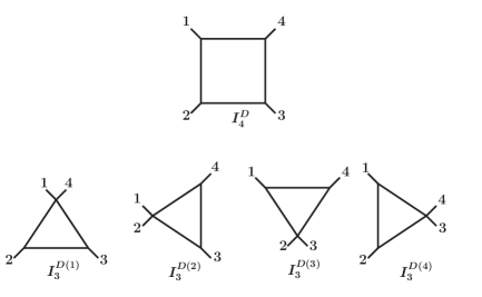
Figure 23: The $D$-dimensional box integral and its four triangle-integral daughters.

Using Eq. (289), we can reduce an expression that contains higher-dimensional integrals to one that does not. For the reverse process, i.e. in order to eliminate all $\epsilon$ and $m$ dependence in a one-loop amplitude $\mathcal{M}_{4}^{\text{1-loop}}$, we adopt the following strategy: We start by inspecting the coefficients of the boxes, which take the following schematic form

$$\begin{split}\mathcal{M}_{4}^{\text{1-loop}}&=\frac{P(\epsilon)Q(s,t,m)}{(4-(4-2\epsilon)-1)(4-(6-2\epsilon)-1)(4-(8-2\epsilon)-1)(4-(10-2\epsilon)-1)}I_{4}\\ &+\ldots\end{split}$$ (292)

where $P(\epsilon)$ is at most an order-four polynomial in $\epsilon$ that does not cancel any of the poles of the expression and $Q(s,t,m)$ is some rational function. The maximum degree in $\epsilon$ is directly tied to the maximal power of loop momentum that can appear in the numerator for minimally-coupled gravity. Here we assume the highest possible power of loop momentum, which corresponds to a spin-0 particle circulating in the loop. $I_{4}$ in Eq. (292) stands for a box integral in our amplitude, whose arguments we do not specify since we are being schematic. This discussion applies to all box integrals in our amplitude. The ellipsis contains other master integrals and their coefficients. Looking at Eq. (289), we may identify this term as coming from the $I_{4}^{12-2\epsilon}$ integral,

$$\mathcal{M}_{4}^{\text{1-loop}}=P(\epsilon)Q^{\prime}(s,t,m)I_{4}^{12-2\epsilon}+\ldots\,,$$ (293)

where $Q^{\prime}(s,t,m)$ is some new rational function. Note that the ellipsis also changes as dictated by Eq. (289). Now we may set $D=4-2\epsilon$ in Eq. (289) and rewrite it as follows,

$$\epsilon I_{n}^{6-2\epsilon}=\frac{1}{2c_{0}}[2I_{n}-\sum_{i=1}^{n}c_{i}I_{n-1}^{(i)}-c_{0}(n-5)I_{n}^{6-2\epsilon}]\,,$$ (294)

where $I_{n}^{4-2\epsilon}\equiv I_{n}$. Similarly, setting $D=6-2\epsilon$ in Eq. (289) we get

$$\epsilon I_{n}^{8-2\epsilon}=\frac{1}{2c_{0}}[2I_{n}^{6-2\epsilon}-\sum_{i=1}^{n}c_{i}I_{n-1}^{6-2\epsilon(i)}-c_{0}(n-7)I_{n}^{8-2\epsilon}]\,,$$ (295)

etc. Combining the two we may trade for example $\epsilon^{2}I_{n}^{8-2\epsilon}$ for an expression containing $I_{n}^{8-2\epsilon}$, $I_{n}^{6-2\epsilon}$, $I_{n}$ and lower-point integrals with $\epsilon$ dependence only in the coefficients of the lower-point integrals. In this fashion we turn Eq. (293) into

$$\mathcal{M}_{4}^{\text{1-loop}}=\sum_{r=0}^{4}Q_{r}(s,t)I_{4}^{4+2r-2\epsilon}+\ldots$$ (296)

with some different rational functions $Q_{r}(s,t)$. In this way we eliminate all explicit $\epsilon$ and $m$ dependence in the coefficients of the boxes (we discuss the $m$ dependence momentarily). Only after this step is completed, the poles in $\epsilon$ in the coefficients of the triangles have a similar interpretation, i.e. as coming from higher-dimensional triangles. This is because there is a feed down from the coefficients of the boxes to those of the triangles due to Eq. (289). The fact that the poles of the triangles align correctly is a nontrivial check of our calculation. We repeat this process sequentially for all lower-point integrals to completely remove the explicit $\epsilon$ and $m$ dependence in the coefficients.

This procedure always succeeds. The reason is that there exists an alternative process of reducing the integrals to master integrals that does not introduce any explicit $\epsilon$ dependence, but instead introduces these higher-dimensional integrals (for an extensive discussion we refer the reader to Appendix I of Ref. Bern:1995ix ). The existence of such a process guarantees the success of a procedure like the one outlined above. In addition, we may understand why there is no $m$ dependence in the coefficients of the master integrals in this basis as follows: We imagine performing the calculation in a covariant gauge, in which all propagators in the integrals have the canonical form $(p^{2}-m^{2})$, and there are no other poles in the loop momentum or the mass. We use

$$m^{2}=L^{2}-(L^{2}-m^{2})\,,\quad\quad\mu^{2}=-L^{2}+\ell^{2}$$ (297)

to trade all $m$ and $\mu$ dependence in the coefficients for tensor integrals and lower-point integrals. Once all $m$ and $\mu$ dependence has been eliminated in this way, we may reduce the tensor integrals using the IBP reduction procedure described in Appendix I of Ref. Bern:1995ix . The resulting expression contains higher-dimensional integrals without $\epsilon$ or $m$ dependence.

Appendix H High-order expansion of the one-loop four-graviton amplitudes in the large-mass limit

In this appendix, we present the large-mass expansion of our one-loop four-graviton amplitudes through $\mathcal{O}(m^{-20})$. The same results are collected in a Mathematica ancillary file AttachedFile . We give the amplitudes in terms of loop integrals in Appendix F. We obtain the results of this appendix by expanding the ones of Appendix F in the large-mass limit. We give the values and expansion of the integrals in Appendix G.1. The present representation corresponds to low-energy effective description of the gravitational theories under consideration.

The data contained here should be useful for systematic investigations at higher orders in the $1/m$ expansion than carried out in this paper. The examples in Sects. V-VI based on low orders in the expansion suggest that Wilson coefficients in physical theories lie on small islands in the allowed parameter space. Rather strikingly, these islands are one dimensional to a good approximation, which is due to the LSD property. Rather remarkably the string-theory data we use also satisfy similar properties, so the Wilson coefficients obtained from string theory also populate these islands. We hope that the data presented here will facilitate further investigations of these features.

Using the amplitudes expanded in the large-mass limit one may obtain the low-energy effective description of the theory, along the lines of Sect. III. Besides the operators present in the action of Eq. (66), one should include operators of the schematic form $D^{2k}R^{4}$. The operators $D^{2k}R^{4}$ correspond to the terms of $\mathcal{O}(m^{-(4+2k)})$.

We organize the amplitudes in a supersymmetric decomposition (32) in terms of the new contributions for a given spin, $\mathcal{M}_{4}^{\{\it S\}}$. We may then assemble these pieces into the contributions for a particle of a given spin circulating in the loop using Eq. (32). Regarding the double-minus configuration, starting with the spin-0 contribution and moving to the additional new pieces through spin 2, we have,

$$f^{\{0\}} (s,u)=\mathcal{K}\Bigg{(}\frac{1}{6300m^{4}}+\frac{t}{41580m^{6}}$$

$$+\frac{81(s^{2}+u^{2})+155su}{15135120m^{8}}+\frac{t\big{(}161(s^{2}+u^{2})+324su\big{)}}{151351200m^{10}}$$

$$+\frac{3556(s^{4}+u^{4})+14035(s^{3}u+su^{3})+21030s^{2}u^{2}}{15437822400m^{12}}$$

$$+\frac{t\big{(}2052(s^{4}+u^{4})+8218(s^{3}u+su^{3})+12287s^{2}u^{2}\big{)}}{41902660800m^{14}}$$

$$+\frac{4634(s^{6}+u^{6})+27650(s^{5}u+su^{5})+69026(s^{4}u^{2}+s^{2}u^{4})+91987s^{3}u^{3}}{430200650880m^{16}}$$

$$+\frac{t\big{(}87780(s^{6}+u^{6})+526770(s^{5}u+su^{5})+1314684(s^{4}u^{2}+s^{2}u^{4})+1752653s^{3}u^{3}\big{)}}{37104806138400m^{18}}$$

$$+\frac{2551824(s^{8}+u^{8})+20357964(s^{7}u+su^{7})+71183961(s^{6}u^{2}+s^{2}u^{6})}{4823624797992000m^{20}}$$

$$+\frac{142285437(s^{5}u^{3}+s^{3}u^{5})+177823240s^{4}u^{4}}{4823624797992000m^{20}}\Bigg{)}\,,$$ (298)

$$f^{\{1/2\}} (s,u)=\mathcal{K}\Bigg{(}\frac{1}{1120m^{4}}+\frac{t}{8400m^{6}}$$

$$+\frac{15(s^{2}+u^{2})+28su}{554400m^{8}}+\frac{t\big{(}153(s^{2}+u^{2})+313su\big{)}}{30270240m^{10}}$$

$$+\frac{665(s^{4}+u^{4})+2596(s^{3}u+su^{3})+3890s^{2}u^{2}}{605404800m^{12}}$$

$$+\frac{t\big{(}581(s^{4}+u^{4})+2345(s^{3}u+su^{3})+3495s^{2}u^{2}\big{)}}{2572970400m^{14}}$$

$$+\frac{29106(s^{6}+u^{6})+172676(s^{5}u+su^{5})+430955(s^{4}u^{2}+s^{2}u^{4})+574230s^{3}u^{3}}{586637251200m^{16}}$$

$$+\frac{t\big{(}34440(s^{6}+u^{6})+207564(s^{5}u+su^{5})+517436(s^{4}u^{2}+s^{2}u^{4})+690109s^{3}u^{3}\big{)}}{3226504881600m^{18}}$$

$$+\frac{39270(s^{8}+u^{8})+312240(s^{7}u+su^{7})+1091604(s^{6}u^{2}+s^{2}u^{6})}{16491024950400m^{20}}$$

$$+\frac{2181716(s^{5}u^{3}+s^{3}u^{5})+2726549s^{4}u^{4}}{16491024950400m^{20}}\Bigg{)}\,,$$ (299)

$$f^{\{1\}} (s,u)=\mathcal{K}\Bigg{(}\frac{1}{180m^{4}}+\frac{t}{1680m^{6}}$$

$$+\frac{22(s^{2}+u^{2})+39su}{151200m^{8}}+\frac{t\big{(}20(s^{2}+u^{2})+43su\big{)}}{831600m^{10}}$$

$$+\frac{825(s^{4}+u^{4})+3125(s^{3}u+su^{3})+4684s^{2}u^{2}}{151351200m^{12}}$$

$$+\frac{t\big{(}315(s^{4}+u^{4})+1308(s^{3}u+su^{3})+1930s^{2}u^{2}\big{)}}{302702400m^{14}}$$

$$+\frac{1036(s^{6}+u^{6})+6027(s^{5}u+su^{5})+15036(s^{4}u^{2}+s^{2}u^{4})+20030s^{3}u^{3}}{4410806400m^{16}}$$

$$+\frac{t\big{(}7056(s^{6}+u^{6})+43316(s^{5}u+su^{5})+107555(s^{4}u^{2}+s^{2}u^{4})+143715s^{3}u^{3}\big{)}}{146659312800m^{18}}$$

$$+\frac{11760(s^{8}+u^{8})+92232(s^{7}u+su^{7})+322372(s^{6}u^{2}+s^{2}u^{6})}{1075501627200m^{20}}$$

$$+\frac{644205(s^{5}u^{3}+s^{3}u^{5})+805050s^{4}u^{4}}{1075501627200m^{20}}\Bigg{)}\,,$$ (300)

$$f^{\{3/2\}} (s,u)=\mathcal{K}\Bigg{(}\frac{1}{24m^{4}}+\frac{t}{360m^{6}}$$

$$+\frac{9(s^{2}+u^{2})+14su}{10080m^{8}}+\frac{t\big{(}8(s^{2}+u^{2})+21su\big{)}}{75600m^{10}}$$

$$+\frac{10(s^{4}+u^{4})+34(s^{3}u+su^{3})+51s^{2}u^{2}}{332640m^{12}}$$

$$+\frac{t\big{(}225(s^{4}+u^{4})+1075(s^{3}u+su^{3})+1518s^{2}u^{2}\big{)}}{50450400m^{14}}$$

$$+\frac{105(s^{6}+u^{6})+558(s^{5}u+su^{5})+1391(s^{4}u^{2}+s^{2}u^{4})+1852s^{3}u^{3}}{86486400m^{16}}$$

$$+\frac{t\big{(}224(s^{6}+u^{6})+1533(s^{5}u+su^{5})+3729(s^{4}u^{2}+s^{2}u^{4})+5035s^{3}u^{3}\big{)}}{1102701600m^{18}}$$

$$+\frac{5292(s^{8}+u^{8})+38416(s^{7}u+su^{7})+134211(s^{6}u^{2}+s^{2}u^{6})}{97772875200m^{20}}$$

$$+\frac{268122(s^{5}u^{3}+s^{3}u^{5})+335050s^{4}u^{4}}{97772875200m^{20}}\Bigg{)}\,,$$ (301)

$$f^{\{2\}} (s,u)=\mathcal{K}\Bigg{(}\frac{1}{2m^{4}}+\frac{s^{2}+su+u^{2}}{120m^{8}}$$

$$+\frac{stu}{504m^{10}}+\frac{(s^{2}+su+u^{2})^{2}}{3780m^{12}}+\frac{(s^{2}+su+u^{2})stu}{7920m^{14}}$$

$$+\frac{75(s^{6}+u^{6})+225(s^{5}u+su^{5})+559(s^{4}u^{2}+s^{2}u^{4})+743s^{3}u^{3}}{7207200m^{16}}$$

$$+\frac{3(s^{2}+su+u^{2})^{2}stu}{400400m^{18}}$$

$$+\frac{(s^{2}+su+u^{2})(56(s^{6}+u^{6})+168(s^{5}u+su^{5})+557(s^{4}u^{2}+s^{2}u^{4})+834s^{3}u^{3})}{122522400m^{20}}\Bigg{)}\,.$$ (302)

We give the relation between $\mathcal{M}_{4}(1^{+},2^{-},3^{-},4^{+})$ and $f(s,u)$ in Eq. (68) and define $\mathcal{K}$ in Eq. (87).

For the all-plus and single-minus configurations it suffices to give the result for the spin-0 contribution since we obtain the remaining amplitudes via Eq. (34). For the all-plus configuration we have

$$h^{S=0} (s,u)=\mathcal{K}\Bigg{(}\frac{stu}{504m^{2}}+\frac{(s^{2}+su+u^{2})^{2}}{3780m^{4}}$$

$$+\frac{(s^{2}+su+u^{2})stu}{7920m^{6}}+\frac{75(s^{6}+u^{6})+225(s^{5}u+su^{5})+559(s^{4}u^{2}+s^{2}u^{4})+743s^{3}u^{3}}{7207200m^{8}}$$

$$+\frac{3(s^{2}+su+u^{2})^{2}stu}{400400m^{10}}$$

$$+\frac{(s^{2}+su+u^{2})\big{(}56(s^{6}+u^{6})+168(s^{5}u+su^{5})+557(s^{4}u^{2}+s^{2}u^{4})+834s^{3}u^{3}\big{)}}{122522400m^{12}}$$

$$+\frac{\big{(}392(s^{6}+u^{6})+1176(s^{5}u+su^{5})+2481(s^{4}u^{2}+s^{2}u^{4})+3002s^{3}u^{3}\big{)}stu}{888844320m^{14}}$$

$$+\frac{(s^{2}+su+u^{2})^{2}\big{(}105(s^{6}+u^{6})+315(s^{5}u+su^{5})+1412(s^{4}u^{2}+s^{2}u^{4})+2299s^{3}u^{3}\big{)}}{4888643760m^{16}}$$

$$+\frac{(s^{2}+su+u^{2})\big{(}150(s^{6}+u^{6})+450(s^{5}u+su^{5})+1049(s^{4}u^{2}+s^{2}u^{4})+1348s^{3}u^{3}\big{)}stu}{5766092640m^{18}}$$

$$+\frac{1}{33731641944000m^{20}}\Big{(}35640(s^{12}+u^{12})$$

$$\hskip 56.9055pt\hbox{}+213840(s^{11}u+su^{11})+1174365(s^{10}u^{2}+s^{2}u^{10})+3911625(s^{9}u^{3}+s^{3}u^{9})$$

$$\hskip 56.9055pt\hbox{}+8797526(s^{8}u^{4}+s^{4}u^{8})+14072594(s^{7}u^{5}+s^{5}u^{7})+16416696s^{6}u^{6}\Big{)}\Bigg{)}\,,$$ (303)

while for the single-minus configuration we find

$$g^{S=0} (s,u)=\mathcal{K}\Bigg{(}\frac{1}{5040m^{2}stu}+\frac{1}{6306300m^{8}}$$

$$+\frac{(s^{2}+su+u^{2})}{441080640m^{12}}+\frac{stu}{2715913200m^{14}}+\frac{(s^{2}+su+u^{2})^{2}}{22406283900m^{16}}+\frac{(s^{2}+su+u^{2})stu}{64250746560m^{18}}$$

$$+\frac{\big{(}27(s^{6}+u^{6})+81(s^{5}u+su^{5})+197(s^{4}u^{2}+s^{2}u^{4})+259s^{3}u^{3}\big{)}}{25057791158400m^{20}}\Bigg{)}\,.$$ (304)

The relation of $\mathcal{M}_{4}(1^{+},2^{+},3^{+},4^{+})$ and $\mathcal{M}_{4}(1^{+},2^{+},3^{-},4^{+})$ to $h(s,u)$ and $g(s,u)$ is found in Eq. (68).

References

-
(1)
Y. Aharonov, A. Komar and L. Susskind,
Phys. Rev. 182, 1400-1403 (1969);
A. Adams, N. Arkani-Hamed, S. Dubovsky, A. Nicolis and R. Rattazzi, JHEP 10, 014 (2006) [arXiv:hep-th/0602178 [hep-th]];
J. Distler, B. Grinstein, R. A. Porto and I. Z. Rothstein, Phys. Rev. Lett. 98, 041601 (2007) [arXiv:hep-ph/0604255 [hep-ph]];
A. Gruzinov and M. Kleban, Class. Quant. Grav. 24, 3521-3524 (2007) [arXiv:hep-th/0612015 [hep-th]];
L. Vecchi, JHEP 11, 054 (2007) [arXiv:0704.1900 [hep-ph]];
I. Low, R. Rattazzi and A. Vichi, JHEP 04, 126 (2010) [arXiv:0907.5413 [hep-ph]];
A. Nicolis, R. Rattazzi and E. Trincherini, JHEP 05, 095 (2010) [erratum: JHEP 11, 128 (2011)] [arXiv:0912.4258 [hep-th]];
C. Cheung and G. N. Remmen, JHEP 12, 087 (2014) [arXiv:1407.7865 [hep-th]];
D. Baumann, D. Green, H. Lee and R. A. Porto, Phys. Rev. D 93, no.2, 023523 (2016) [arXiv:1502.07304 [hep-th]];
B. Bellazzini, C. Cheung and G. N. Remmen, Phys. Rev. D 93, no.6, 064076 (2016) [arXiv:1509.00851 [hep-th]];
B. Bellazzini, JHEP 02, 034 (2017) [arXiv:1605.06111 [hep-th]];
C. Cheung and G. N. Remmen, Phys. Rev. Lett. 118, no.5, 051601 (2017) [arXiv:1608.02942 [hep-th]];
C. de Rham, S. Melville, A. J. Tolley and S. Y. Zhou, Phys. Rev. D 96, no.8, 081702 (2017) [arXiv:1702.06134 [hep-th]];
C. de Rham, S. Melville, A. J. Tolley and S. Y. Zhou, JHEP 03, 011 (2018) [arXiv:1706.02712 [hep-th]];
C. de Rham and A. J. Tolley, Phys. Rev. D 102, no.8, 084048 (2020) [arXiv:2007.01847 [hep-th]]. - (2) D. Bai and Y. H. Xing, Nucl. Phys. B 932, 15-28 (2018) [arXiv:1610.00241 [hep-th]].
- (3) A. J. Tolley, Z. Y. Wang and S. Y. Zhou, [arXiv:2011.02400 [hep-th]].
- (4) S. Caron-Huot and V. Van Duong, [arXiv:2011.02957 [hep-th]].
- (5) N. Arkani-Hamed, T. C. Huang and Y. T. Huang, [arXiv:2012.15849 [hep-th]].
- (6) A. Sinha and A. Zahed, [arXiv:2012.04877 [hep-th]].
- (7) S. Caron-Huot, D. Mazac, L. Rastelli and D. Simmons-Duffin, [arXiv:2102.08951 [hep-th]].
- (8) P. Benincasa and F. Cachazo, [arXiv:0705.4305 [hep-th]].
- (9) S. Weinberg, Phys. Rev. 135, B1049-B1056 (1964) doi:10.1103/PhysRev.135.B1049 S. Weinberg, Phys. Rev. 138, B988-B1002 (1965) doi:10.1103/PhysRev.138.B988
- (10) Y. t. Huang, J. Y. Liu, L. Rodina and Y. Wang, [arXiv:2008.02293 [hep-th]].
- (11) X. O. Camanho, J. D. Edelstein, J. Maldacena and A. Zhiboedov, JHEP 02, 020 (2016) [arXiv:1407.5597 [hep-th]].
- (12) D. Meltzer and E. Perlmutter, JHEP 07, 157 (2018) [arXiv:1712.04861 [hep-th]].
- (13) A. Belin, D. M. Hofman and G. Mathys, JHEP 08, 032 (2019) [arXiv:1904.05892 [hep-th]].
- (14) M. Kologlu, P. Kravchuk, D. Simmons-Duffin and A. Zhiboedov, [arXiv:1904.05905 [hep-th]].
- (15) J. Kaplan and S. Kundu, [arXiv:2009.08460 [hep-th]].
- (16) S. Caron-Huot, D. Mazac, L. Rastelli and D. Simmons-Duffin, [arXiv:2008.04931 [hep-th]].
- (17) T. Trott, [arXiv:2011.10058 [hep-ph]].
- (18) A. Guerrieri, J. Penedones and P. Vieira, [arXiv:2102.02847 [hep-th]].
- (19) D. C. Dunbar and P. S. Norridge, Nucl. Phys. B 433, 181-208 (1995) [arXiv:hep-th/9408014 [hep-th]].
- (20) Z. Bern and A. G. Morgan, Nucl. Phys. B 467, 479 (1996) [hep-ph/9511336].
-
(21)
Z. Bern, L. J. Dixon, D. C. Dunbar and D. A. Kosower,
Nucl. Phys. B 425, 217-260 (1994)
[arXiv:hep-ph/9403226 [hep-ph]];
Z. Bern, L. J. Dixon, D. C. Dunbar and D. A. Kosower, Nucl. Phys. B 435, 59-101 (1995) [arXiv:hep-ph/9409265 [hep-ph]]. -
(22)
Z. Bern, J. J. M. Carrasco and H. Johansson,
Phys. Rev. D 78, 085011 (2008)
[arXiv:0805.3993 [hep-ph]];
Z. Bern, J. J. M. Carrasco and H. Johansson, Phys. Rev. Lett. 105, 061602 (2010) [arXiv:1004.0476 [hep-th]]. - (23) Z. Bern, J. J. Carrasco, M. Chiodaroli, H. Johansson and R. Roiban, [arXiv:1909.01358 [hep-th]].
- (24) R. Britto and E. Mirabella, JHEP 01, 045 (2012) [arXiv:1109.5106 [hep-ph]].
-
(25)
F. A. Berends, R. Kleiss, P. De Causmaecker, R. Gastmans and T. T. Wu,
Phys. Lett. B 103, 124-128 (1981);
P. De Causmaecker, R. Gastmans, W. Troost and T. T. Wu, Nucl. Phys. B 206, 53-60 (1982);
R. Kleiss and W. Stirling, Nucl. Phys. B 262, 235-262 (1985);
J. Gunion and Z. Kunszt, Phys. Lett. B 161, 333 (1985);
Z. Xu, D. Zhang and L. Chang, Nucl. Phys. B 291, 392-428 (1987). -
(26)
M. L. Mangano and S. J. Parke,
Phys. Rept. 200, 301-367 (1991)
[arXiv:hep-th/0509223 [hep-th]];
L. J. Dixon, [arXiv:hep-ph/9601359 [hep-ph]]. - (27) J.C. Collins, Renormalization, (Cambridge University Press) (1984).
-
(28)
Z. Bern and D. A. Kosower,
Nucl. Phys. B 379, 451-561 (1992);
Z. Bern, A. De Freitas, L. J. Dixon and H. L. Wong, Phys. Rev. D 66, 085002 (2002) [arXiv:hep-ph/0202271 [hep-ph]]. -
(29)
Z. Bern, L. J. Dixon and D. A. Kosower,
Nucl. Phys. B 513, 3-86 (1998)
[arXiv:hep-ph/9708239 [hep-ph]];
Z. Bern, A. De Freitas and L. J. Dixon, JHEP 03, 018 (2002) [arXiv:hep-ph/0201161 [hep-ph]];
A. Broggio, C. Gnendiger, A. Signer, D. Stöckinger and A. Visconti, JHEP 01, 078 (2016) [arXiv:1506.05301 [hep-ph]]. - (30) Z. Bern, L. J. Dixon and D. A. Kosower, Ann. Rev. Nucl. Part. Sci. 46, 109-148 (1996) [arXiv:hep-ph/9602280 [hep-ph]].
- (31) Z. Bern and Y. t. Huang, J. Phys. A 44, 454003 (2011) [arXiv:1103.1869 [hep-th]].
-
(32)
G. Passarino and M. J. G. Veltman,
Nucl. Phys. B 160, 151-207 (1979);
Z. Bern, L. J. Dixon and D. A. Kosower, Nucl. Phys. B 412, 751-816 (1994) [arXiv:hep-ph/9306240 [hep-ph]]. -
(33)
A. V. Smirnov,
JHEP 10, 107 (2008)
[arXiv:0807.3243 [hep-ph]];
A. V. Smirnov and F. S. Chuharev, [arXiv:1901.07808 [hep-ph]]. - (34) R. J. Eden, P. V. Landshoff, D. I. Olive and J. C. Polkinghorne, The analytic S-matrix, Cambridge University Press (1966).
- (35) Z. Bern, L. J. Dixon and D. A. Kosower, JHEP 0408, 012 (2004) [hep-ph/0404293].
-
(36)
Z. Bern, J. J. M. Carrasco, L. J. Dixon, H. Johansson and R. Roiban,
Phys. Rev. D 82, 125040 (2010)
[arXiv:1008.3327 [hep-th]];
Z. Bern, J. J. M. Carrasco, H. Johansson and R. Roiban, Phys. Rev. Lett. 109, 241602 (2012) [arXiv:1207.6666 [hep-th]];
Z. Bern, J. J. Carrasco, W. M. Chen, A. Edison, H. Johansson, J. Parra-Martinez, R. Roiban and M. Zeng, Phys. Rev. D 98, no.8, 086021 (2018) [arXiv:1804.09311 [hep-th]]. -
(37)
D. Forde,
Phys. Rev. D 75, 125019 (2007)
[arXiv:0704.1835 [hep-ph]];
C. F. Berger, Z. Bern, L. J. Dixon, F. Febres Cordero, D. Forde, H. Ita, D. A. Kosower and D. Maitre, Phys. Rev. D 78, 036003 (2008) [arXiv:0803.4180 [hep-ph]]. - (38) H. Kawai, D. Lewellen and S. Tye, Nucl. Phys. B 269, 1-23 (1986)
-
(39)
M. Porrati,
Phys. Lett. B 304, 77-80 (1993)
[arXiv:gr-qc/9301012 [gr-qc]].
A. Cucchieri, M. Porrati and S. Deser,
Phys. Rev. D 51, 4543-4549 (1995)
[arXiv:hep-th/9408073 [hep-th]];
I. Giannakis, J. T. Liu and M. Porrati, Phys. Rev. D 59, 104013 (1999) [arXiv:hep-th/9809142 [hep-th]];
S. Deser and A. Waldron, Nucl. Phys. B 631, 369-387 (2002) [arXiv:hep-th/0112182 [hep-th]];
I. Cortese, R. Rahman and M. Sivakumar, Nucl. Phys. B 879, 143-161 (2014) [arXiv:1307.7710 [hep-th]]. - (40) J. Bonifacio, K. Hinterbichler, A. Joyce and R. A. Rosen, JHEP 06, 075 (2018) [arXiv:1712.10020 [hep-th]].
-
(41)
Z. Bern, L. J. Dixon and D. A. Kosower,
Phys. Rev. Lett. 70, 2677-2680 (1993)
[arXiv:hep-ph/9302280 [hep-ph]];
Z. Bern, L. J. Dixon and D. A. Kosower, Nucl. Phys. B 437, 259-304 (1995) [arXiv:hep-ph/9409393 [hep-ph]]. - (42) Z. Bern and A. G. Morgan, Phys. Rev. D 49, 6155-6163 (1994) [arXiv:hep-ph/9312218 [hep-ph]].
-
(43)
P. Fayet,
Nucl. Phys. B 149, 137 (1979);
F. Quevedo, S. Krippendorf and O. Schlotterer, [arXiv:1011.1491 [hep-th]];
R. H. Boels, JHEP 05, 046 (2010) [arXiv:1003.2989 [hep-th]]. -
(44)
J. M. Henn, S. G. Naculich, H. J. Schnitzer and M. Spradlin,
JHEP 04, 038 (2010)
[arXiv:1001.1358 [hep-th]];
J. M. Henn, S. G. Naculich, H. J. Schnitzer and M. Spradlin, JHEP 08, 002 (2010) [arXiv:1004.5381 [hep-th]];
J. M. Henn, J. Phys. A 44, 454011 (2011) [arXiv:1103.1016 [hep-th]];
N. Craig, H. Elvang, M. Kiermaier and T. Slatyer, JHEP 12, 097 (2011) [arXiv:1104.2050 [hep-th]];
M. Kiermaier, [arXiv:1105.5385 [hep-th]];
H. Elvang, D. Z. Freedman and M. Kiermaier, JHEP 06, 015 (2012) [arXiv:1111.0635 [hep-th]];
A. Herderschee, S. Koren and T. Trott, JHEP 10, 092 (2019) [arXiv:1902.07204 [hep-th]];
A. Herderschee, S. Koren and T. Trott, JHEP 08, 107 (2019) [arXiv:1902.07205 [hep-th]]. - (45) L. F. Alday, J. M. Henn, J. Plefka and T. Schuster, JHEP 01, 077 (2010) [arXiv:0908.0684 [hep-th]].
- (46) A. G. Morgan, Phys. Lett. B 351, 249-256 (1995) [arXiv:hep-ph/9502230 [hep-ph]].
-
(47)
Y. M. Zinovev,
Sov. J. Nucl. Phys. 46, 540 (1987)
[arXiv:hep-th/9512041 [hep-th]];
N. Berkovits and M. M. Leite, Phys. Lett. B 415, 144-148 (1997) [arXiv:hep-th/9709148 [hep-th]];
N. Berkovits and M. M. Leite, Phys. Lett. B 454, 38-42 (1999) [arXiv:hep-th/9812153 [hep-th]];
T. Gregoire, M. D. Schwartz and Y. Shadmi, JHEP 07, 029 (2004) [arXiv:hep-th/0403224 [hep-th]]. - (48) Z. Bern and D. A. Kosower, Nucl. Phys. B 379, 451-561 (1992).
- (49) G. ’t Hooft and M. J. G. Veltman, Nucl. Phys. B 44, 189-213 (1972).
-
(50)
M. T. Grisaru, H. N. Pendleton and P. van Nieuwenhuizen,
Phys. Rev. D 15, 996 (1977);
M. T. Grisaru and H. N. Pendleton, Nucl. Phys. B 124, 81-92 (1977);
S. J. Parke and T. R. Taylor, Phys. Lett. B 157, 81 (1985) [erratum: Phys. Lett. B 174, 465 (1986)];
Z. Bern, L. J. Dixon, D. C. Dunbar, M. Perelstein and J. S. Rozowsky, Nucl. Phys. B 530, 401-456 (1998) [arXiv:hep-th/9802162 [hep-th]]. - (51) N. Arkani-Hamed, T. C. Huang and Y. t. Huang, [arXiv:1709.04891 [hep-th]].
-
(52)
K.G. Chetyrkin and F.V. Tkachov,
Nucl. Phys. B 192, 159 (1981);
S. Laporta, Int. J. Mod. Phys. A 15, 5087-5159 (2000) [arXiv:hep-ph/0102033 [hep-ph]]. - (53) G. ’t Hooft and M. J. G. Veltman, Ann. Inst. H. Poincare Phys. Theor. A 20, 69-94 (1974)
-
(54)
S. Weinberg,
Phys. Rev. 140, B516 (1965);
S. G. Naculich and H. J. Schnitzer, JHEP 1105, 087 (2011) [arXiv:1101.1524 [hep-th]];
R. Akhoury, R. Saotome and G. Sterman, Phys. Rev. D 84, 104040 (2011) [arXiv:1109.0270 [hep-th]]. - (55) S. Abreu, F. Febres Cordero, H. Ita, M. Jaquier, B. Page, M. S. Ruf and V. Sotnikov, Phys. Rev. Lett. 124, no.21, 211601 (2020) [arXiv:2002.12374 [hep-th]].
- (56) P. van Nieuwenhuizen and C. C. Wu, J. Math. Phys. 18, 182 (1977)
- (57) J. Broedel and L. J. Dixon, JHEP 10, 091 (2012) [arXiv:1208.0876 [hep-th]].
- (58) N. Sennett, R. Brito, A. Buonanno, V. Gorbenko and L. Senatore, Phys. Rev. D 102, no.4, 044056 (2020) [arXiv:1912.09917 [gr-qc]].
- (59) S. Endlich, V. Gorbenko, J. Huang and L. Senatore, JHEP 09, 122 (2017) [arXiv:1704.01590 [gr-qc]].
- (60) S. A. Fulling, R. C. King, B. G. Wybourne and C. J. Cummins, Class. Quant. Grav. 9, 1151-1197 (1992)
- (61) D. C. Dunbar, J. H. Godwin, G. R. Jehu and W. B. Perkins, Phys. Lett. B 780, 41-47 (2018) [arXiv:1711.05526 [hep-th]].
- (62) A. Brandhuber and G. Travaglini, JHEP 01, 010 (2020) [arXiv:1905.05657 [hep-th]].
- (63) M. Accettulli Huber, A. Brandhuber, S. De Angelis and G. Travaglini, [arXiv:2006.02375 [hep-th]].
- (64) W. T. Emond and N. Moynihan, JHEP 12, 019 (2019) [arXiv:1905.08213 [hep-th]]; D. J. Burger, W. T. Emond and N. Moynihan, Phys. Rev. D 101, no.8, 084009 (2020) [arXiv:1910.11618 [hep-th]].
- (65) S. D. Chowdhury, A. Gadde, T. Gopalka, I. Halder, L. Janagal and S. Minwalla, JHEP 02, 114 (2020) [arXiv:1910.14392 [hep-th]].
- (66) L. Alberte, C. de Rham, S. Jaitly and A. J. Tolley, [arXiv:2012.05798 [hep-th]].
- (67) A. Hebbar, D. Karateev and J. Penedones, [arXiv:2011.11708 [hep-th]].
- (68) A. Hebbar, K. Häring, D. Karateev, M. Meineri, J. Penedones, work in progress
- (69) A. Strominger, [arXiv:1703.05448 [hep-th]].
- (70) N. Arkani-Hamed, M. Pate, A. M. Raclariu and A. Strominger, [arXiv:2012.04208 [hep-th]].
- (71) A. Martin, Nuovo Cim. A 42, 930-953 (1965) doi:10.1007/BF02720568
- (72) J. Maldacena, S. H. Shenker and D. Stanford, JHEP 08, 106 (2016) doi:10.1007/JHEP08(2016)106 [arXiv:1503.01409 [hep-th]].
- (73) D. Chandorkar, S. D. Chowdhury, S. Kundu and S. Minwalla, [arXiv:2102.03122 [hep-th]].
- (74) S. Caron-Huot, Z. Komargodski, A. Sever and A. Zhiboedov, JHEP 10, 026 (2017) [arXiv:1607.04253 [hep-th]].
- (75) N. Arkani-Hamed, S. Dimopoulos and G. R. Dvali, Phys. Lett. B 429, 263-272 (1998) [arXiv:hep-ph/9803315 [hep-ph]].
- (76) L. Randall and R. Sundrum, Phys. Rev. Lett. 83, 3370-3373 (1999) [arXiv:hep-ph/9905221 [hep-ph]].
- (77) L. Randall and R. Sundrum, Phys. Rev. Lett. 83, 4690-4693 (1999) [arXiv:hep-th/9906064 [hep-th]].
-
(78)
C. Zhang and S. Y. Zhou,
Phys. Rev. Lett. 125, no.20, 201601 (2020)
[arXiv:2005.03047 [hep-ph]];
K. Yamashita, C. Zhang and S. Y. Zhou, JHEP 01, 095 (2021) [arXiv:2009.04490 [hep-ph]]. - (79) B. Bellazzini, J. Elias Miró, R. Rattazzi, M. Riembau and F. Riva, [arXiv:2011.00037 [hep-th]].
- (80) R. C. Brower, J. Polchinski, M. J. Strassler and C. I. Tan, JHEP 12, 005 (2007) [arXiv:hep-th/0603115 [hep-th]].
- (81) Z. Bern and G. Chalmers, Nucl. Phys. B 447, 465 (1995) [hep-ph/9503236].
-
(82)
N. Arkani-Hamed, L. Motl, A. Nicolis and C. Vafa,
JHEP 06, 060 (2007)
[arXiv:hep-th/0601001 [hep-th]];
H. Ooguri and C. Vafa, Nucl. Phys. B 766, 21-33 (2007) [arXiv:hep-th/0605264 [hep-th]];
T. D. Brennan, F. Carta and C. Vafa, PoS TASI2017, 015 (2017) [arXiv:1711.00864 [hep-th]];
E. Palti, Fortsch. Phys. 67, no.6, 1900037 (2019) [arXiv:1903.06239 [hep-th]];
M. van Beest, J. Calderón-Infante, D. Mirfendereski and I. Valenzuela, [arXiv:2102.01111 [hep-th]]. -
(83)
A. Bissi, P. Dey and T. Hansen,
JHEP 04, 092 (2020)
doi:10.1007/JHEP04(2020)092
[arXiv:1910.04661 [hep-th]];
D. Carmi and S. Caron-Huot, JHEP 09, 009 (2020) [arXiv:1910.12123 [hep-th]];
D. Mazáč, L. Rastelli and X. Zhou, [arXiv:1910.12855 [hep-th]];
J. Penedones, J. A. Silva and A. Zhiboedov, JHEP 08, 031 (2020) [arXiv:1912.11100 [hep-th]];
S. Caron-Huot, D. Mazac, L. Rastelli and D. Simmons-Duffin, [arXiv:2008.04931 [hep-th]]. - (84) N. Afkhami-Jeddi, S. Kundu and A. Tajdini, JHEP 10, 156 (2018) [arXiv:1805.07393 [hep-th]].
- (85) N. Afkhami-Jeddi, S. Kundu and A. Tajdini, JHEP 04, 056 (2019) [arXiv:1811.01952 [hep-th]].
- (86) M. E. Peskin and D. V. Schroeder, An Introduction to quantum field theory CRC Press (1995).
-
(87)
L. P. S. Singh and C. R. Hagen,
Phys. Rev. D 9, 898-909 (1974);
Z. Bern, A. Luna, R. Roiban, C. H. Shen and M. Zeng, [arXiv:2005.03071 [hep-th]]. - (88) W. Pauli and M. Fierz, Helv. Phys. Acta 12, 297-300 (1939)
- (89) Z. Bern, D. C. Dunbar and T. Shimada, Phys. Lett. B 312, 277-284 (1993) [arXiv:hep-th/9307001 [hep-th]].
- (90) M. Correia, A. Sever and A. Zhiboedov, [arXiv:2006.08221 [hep-th]].
- (91) See the ancillary files of this manuscript.
-
(92)
L. M. Brown and R. P. Feynman,
Phys. Rev. 85, 231-244 (1952);
L. M. Brown, Nuovo Cim. 22, no.1, 178-182 (1961);
B. Petersson, J. Math. Phys. 6, 1955-1959 (1965);
D. B. Melrose, Nuovo Cim. 40, 181-213 (1965);
G. ’t Hooft and M. J. G. Veltman, Nucl. Phys. B 153, 365-401 (1979);
W. L. van Neerven and J. A. M. Vermaseren, Phys. Lett. B 137, 241-244 (1984);
R. G. Stuart, Comput. Phys. Commun. 48, 367-389 (1988);
G. J. van Oldenborgh and J. A. M. Vermaseren, Z. Phys. C 46, 425-438 (1990);
A. Denner, U. Nierste and R. Scharf, Nucl. Phys. B 367, 637-656 (1991);
A. I. Davydychev, [arXiv:hep-ph/9307323 [hep-ph]]. -
(93)
Z. Bern, L. J. Dixon and D. A. Kosower,
Phys. Lett. B 302, 299 (1993)
Erratum: [Phys. Lett. B 318, 649 (1993)]
[hep-ph/9212308];
Z. Bern, L. J. Dixon and D. A. Kosower, Nucl. Phys. B 412, 751-816 (1994) [arXiv:hep-ph/9306240 [hep-ph]].