Policy Information Capacity:
Information-Theoretic Measure for Task Complexity
in Deep Reinforcement Learning

Abstract

Progress in deep reinforcement learning (RL) research is largely enabled by benchmark task environments. However, analyzing the nature of those environments is often overlooked. In particular, we still do not have agreeable ways to measure the difficulty or solvability of a task, given that each has fundamentally different actions, observations, dynamics, rewards, and can be tackled with diverse RL algorithms. In this work, we propose policy information capacity (PIC) – the mutual information between policy parameters and episodic return – and policy-optimal information capacity (POIC) – between policy parameters and episodic optimality – as two environment-agnostic, algorithm-agnostic quantitative metrics for task difficulty. Evaluating our metrics across toy environments as well as continuous control benchmark tasks from OpenAI Gym and DeepMind Control Suite, we empirically demonstrate that these information-theoretic metrics have higher correlations with normalized task solvability scores than a variety of alternatives. Lastly, we show that these metrics can also be used for fast and compute-efficient optimizations of key design parameters such as reward shaping, policy architectures, and MDP properties for better solvability by RL algorithms without ever running full RL experiments.

1 Introduction

The myriad recent successes of reinforcement learning (RL) have arguably been enabled by the proliferation of deep neural network function approximators applied to rich observational inputs (Mnih et al., 2015; Hessel et al., 2018; Kalashnikov et al., 2018), enabling an agent to adeptly manage long-term sequential decision making in complex environments. While in the past much of the empirical RL research has focused on tabular or linear function approximation case (Dietterich, 1998; McGovern & Barto, 2001; Konidaris & Barto, 2009), the impressive successes of recent years (and anticipation of domains ripe for subsequent successes) has spurred the creation of non-tabular benchmarks – i.e., continuous control and/or continuous observation – in which neural network function approximators are effectively a prerequisite (Bellemare et al., 2013; Brockman et al., 2016; Tassa et al., 2018). Accordingly, empirical RL research is presently heavily focused on the use of neural network function approximators, spurring new algorithmic developments in both model-free (Mnih et al., 2015; Schulman et al., 2015; Lillicrap et al., 2016; Gu et al., 2016b, 2017; Haarnoja et al., 2018) and model-based (Chua et al., 2018; Janner et al., 2019; Hafner et al., 2020a) RL.

Despite the impressive progress of RL algorithms, the analysis of the RL environments has been difficult and stagnant, precisely due to the complexity of modern benchmarks and neural network architectures required to solve them. Most prior works analyzing sample complexity (a common measure of task complexity) focus on tabular MDPs with finite state and action dimensionalities (Strehl et al., 2006, 2009) or MDPs with simple dynamics (Recht, 2018), and are not applicable or measurable for typical deep RL benchmark tasks. Besides the fact that the components of the environments – observations, actions, dynamics, and rewards – are drastically different in typical benchmarks, the investigation into task solvability is further complicated by the diversity of deep RL algorithms used in practice (Schulman et al., 2015; Lillicrap et al., 2016; Gu et al., 2016b, a, 2017; Haarnoja et al., 2018; Chua et al., 2018; Salimans et al., 2017), where each algorithm has distinct convergence behaviors. Coming up with a universal, scalable, and measurable definition for task complexity of an RL environment appears an impossible task.

In this work, we propose policy information capacity (PIC) and policy-optimal information capacity (POIC) as practical metrics for task or environment complexity, taking inspiration from information-theoretic RL research – particularly mutual information maximization or empowerment (Klyubin et al., 2005; Tishby & Polani, 2011; Jung et al., 2011; Mohamed & Rezende, 2015; Eysenbach et al., 2019; Warde-Farley et al., 2019; Sharma et al., 2020b; Hafner et al., 2020b). Policy information capacity measures mutual information between policy parameters and cumulative episodic rewards. As with standard decomposition in mutual information, maximizing policy information capacity corresponds to maximizing reward marginal entropy through policies (diversity maximization) while minimizing reward conditional entropy conditioned on any given policy parameter (predictability maximization), and effectively corresponds to maximizing reward controllability. Intuitively, if an agent can easily control rewards or relevant states that affect the cumulative rewards, then most RL algorithms can generally maximize the rewards easily and the environment should be classified as “easy”. Alternatively, policy-optimal information capacity (POIC), a variant of PIC drawing on the control as inference literature (Todorov et al., 2006; Toussaint & Storkey, 2006; Rawlik et al., 2012; Fox et al., 2016; Jaques et al., 2017; Haarnoja et al., 2017; Levine, 2018), measures mutual information between policy parameters and whether an episode is optimal or not, and even more closely relates to the optimizability of an RL environment.

We compute policy and policy-optimal information capacities across a range of benchmark environments (Brockman et al., 2016; Tassa et al., 2018), and show that, in practice, especially POIC has a higher correlation with normalized task scores (computed as a brute-force proxy for task complexity by executing many runs of RL algorithms) than other sensible alternatives. Considering the simplicity of our metrics and the drastically varied nature of the benchmarks, our result shows that PIC and POIC can serve as practical and measurable metrics for task complexity.

In summary, our work makes the following contributions:

• We define and propose policy information capacity (PIC) and its variant, policy-optimal information capacity (POIC) as algorithm-agnostic quantitative metrics for measuring task complexity, and show that, POIC in particular corresponds well with empirical task solvability computed across diverse benchmark environments (Brockman et al., 2016; Tassa et al., 2018).

• We set up the first quantitative experimental protocol to evaluate the correctness of a task complexity metric.

• We show that both PIC and POIC can be used as fast proxies for tuning experimental parameters to improve learning progress, such as reward shaping, or policy architectures and initialization parameters, without running any full RL experiment.

2 Related Work

We provide a brief overview of related works, first of previously proposed proxy metrics for assessing the properties of RL algorithms or environments, and then of instances of mutual information (MI) in the context of RL.

Analysis of RL Environments

A large body of prior work has sought to theoretically analyze RL algorithms, as opposed to RL environments. For example, Kearns & Singh (2002); Strehl et al. (2009); Dann & Brunskill (2015) derive sample complexity bounds under a finite MDP setting, while Jaksch et al. (2010); Azar et al. (2017); Jin et al. (2018) and Jin et al. (2020) prove regret bounds under finite MDP and linear function approximation settings respectively. Some recent works extend these previous results to non-linear function approximation (Du et al., 2019; Wang et al., 2020; Yang et al., 2020), but they require strong assumptions on function approximators, such as a low Eluder dimension or infinitely-wide neural networks. All these works, however, are algorithm-specific and do not study the properties of RL environments or MDPs.

Asides from algorithms, there are theoretical works that directly study the properties of MDPs. Jaksch et al. (2010) consider the diameter of an MDP, which is the maximum over distinct state pairs $(s,s^{\prime})$ of expected steps to reach $s^{\prime}$ from $s$. Jiang et al. (2017) propose Bellman rank and show that an MDP with a low Bellman rank can be provably-efficiently solved. Maillard et al. (2014) propose the environmental norm, the one-step variance of an optimal state-value function. However, those metrics are often intractable to estimate in practical problems, where state or action dimensions are high dimensional (Jaksch et al., 2010; Pong et al., 2018), neural network function approximations are used (Jiang et al., 2017; Dann et al., 2018), or oracle Q-functions are not computable (Jaksch et al., 2010; Jiang et al., 2017; Maillard et al., 2014). Orthogonally to all these works, we propose tractable metrics that can be approximated numerically for complex RL environments with high-dimensional states and actions and, crucially, complex function approximators such as neural networks.

The recent work of Oller et al. (2020) is the closest to ours, where they qualitatively visualize marginal reward distributions and show how their variances are intuitively related to environment-specific task difficulty scores estimated from a random search algorithm. While they present very promising early results for tackling this ambitious problem, ours has a few critical differences from their work, which we detail in Section 3.2.

Mutual Information

Mutual information has been widely used in RL algorithm development, as a mechanism to encourage emergence of diverse behaviors, sometimes known as empowerment (Klyubin et al., 2005; Tishby & Polani, 2011; Jung et al., 2011; Mohamed & Rezende, 2015). Gregor et al. (2016) employ such diverse behaviors as intrinsic-motivation-based exploration methods, which intend to reach diverse states per option, maximizing the lower bound of mutual information between option and trajectory. Related to exploration (Leibfried et al., 2019; Pong et al., 2020), recently MI-based skill discovery has become a popular topic (Florensa et al., 2017; Eysenbach et al., 2019; Warde-Farley et al., 2019; Nachum et al., 2019; Sharma et al., 2020b, a; Campos et al., 2020; Hansen et al., 2020), and these previous works are sources of inspiration for our own metrics, PIC and POIC. For instance, Eysenbach et al. (2019) and Warde-Farley et al. (2019) learn diverse behaviors through maximizing a lower bound on mutual information between skills and future states, which encourages the agent to learn many distinct skills. In other words, the agents learn how to control the environments (future states) via maximization of mutual information. This intuition – that mutual information is related to the controllability of the environments – motivates our own MI-based task solvability metrics, where our metrics PIC and POIC can be seen as reward and optimality empowerments respectively.

3 Preliminaries

We consider standard RL settings with a Markov Decision Process (MDP) $\mathcal{M}$ defined by state space $\mathcal{S}$, action space $\mathcal{A}$, transition probability $p(s_{t+1}|s_{t},a_{t})$, initial state distribution $p(s_{1})$, and reward function $r(s_{t},a_{t})$. A policy $\pi(a|s)\in\Pi$ maps from states to probability distributions over actions. With function approximation, this policy is parameterized by $\theta\in\mathbb{R}^{d}$, initialized by sampling from a prior distribution of the parameter $p(\theta)$. We use the upper case $\Theta$ to represent this random variable. We also denote a trajectory as $\tau:=(s_{1},a_{1},s_{2},a_{2},...,s_{T})$, and a cumulative reward as $r(\tau):=\sum_{(s,a)\in\tau}r(s,a)$; when clear from the context, we slightly abuse notation and simply use $r$ for $r(\tau)$. We use the upper case $R$ to represent the random variable taking on value $r(\tau)$. Since we focus on evaluation of the environments, we omit a discount factor $\gamma\in[0,1)$.

The distributions $p(r)$ and $p(r|\theta)$ may be factored as,

$$p(r)=\mathbb{E}_{p(\tau|\theta)p(\theta)}\left[p(r|\tau)\right],~{}p(r|\theta)=\mathbb{E}_{p(\tau|\theta)}\left[p(r|\tau)\right],$$

where $p(r|\tau)$ is the reward distribution over trajectory, which, for simplicity, we assume is a deterministic delta distribution, and the marginal distribution of the trajectory conditioned on $\theta$ is $p(\tau|\theta)=\textstyle p(s_{1})\prod_{t=1}^{T}p(s_{t+1}|s_{t},a_{t})\pi(a_{t}|s_{t},\theta)$ .

3.1 Optimality Variable

RL concerns with not only characterization of reward distribution, but also its maximization. Information-theoretic perspective on RL, or control as inference (Todorov et al., 2006; Toussaint & Storkey, 2006; Fox et al., 2016; Jaques et al., 2017; Levine, 2018), connects such maximization with probabilistic inference through the notion of “optimality” variable, a binary random variable $\mathcal{O}_{t}\in\{0,1\}$ in MDP, where $\mathcal{O}_{t}=1$ means the agent behaves “optimally” at time-step $t$, and $\mathcal{O}_{t}=0$ means not optimal. For simplicity, we denote $\mathcal{O}_{1:T}$ as $\mathcal{O}$, which is also a binary random variable, representing whether the agent behaves optimally during the entire episode. We define the distribution of this variable as: $p(\mathcal{O}=1|\tau)=\exp\left((r-r_{\max})/\eta\right)$ , where $\eta>0$ is a temperature and $r_{\max}$ is the maximum return on the MDP. Note that we subtract $r_{\max}$ to ensure $p(\mathcal{O}|\tau)$ is an appropriate probability distribution.

3.2 Random Weight Guessing

Oller et al. (2020) recently proposed a qualitative analysis protocol of environment complexity with function approximation via random weight guessing. It obtains $N$ particles of $\theta$ from prior $p(\theta)$ and runs the deterministic policy $\pi(a_{t}|s_{t},\theta)$ with $M$ episodes per parameter without any training. They qualitatively observe that the mean, percentiles, and variance of episodic returns have certain relations with an approximate difficulty of finding a good policy through random search.

However, our work has a number of key differences from their work: (1) we propose a detailed quantitative evaluation protocol for verifying task difficulty metrics while they focus on qualitative discussions; (2) we derive our main task difficulty metric based on a mixture of SoTA RL algorithms, instead of random search, to better reflect the diversity of algorithm choices in practice; (3) we estimate reward entropies non-parametrically with many particles to reduce approximation errors, while their variance metric assumes Gaussianity of reward distributions and poorly approximates in the case of multi-modality; and (4) we verify the metrics on more diverse set of benchmark environments including OpenAI MuJoCo (Brockman et al., 2016) and DeepMind Control Suite (Tassa et al., 2018) while they evaluate on classic control problems only.

4 Policy and Policy-Optimal Information Capacity

We now introduce our own proposed task complexity metrics. We begin with formal definitions for both metrics, and then provide details on how to estimate them.

4.1 Formal Definitions

Policy Information Capacity (PIC)

We define PIC as the mutual information $\mathcal{I}(\cdot;\cdot)$ between cumulative reward $R$ and policy parameter $\Theta$:

$$\mathcal{I}(R;\Theta)=\mathcal{H}(R)-\mathbb{E}_{p(\theta)}\left[\mathcal{H}(R|\Theta=\theta)\right],$$ (1)

where $\mathcal{H}(\cdot)$ is Shannon entropy. The intuitive interpretation is that when the environment gives a more diverse reward signal (first term in Equation 1) and a more consistent reward signal per parameter (second term), it enables the agent to learn better behaviors.

Policy-Optimal Information Capacity (POIC)

We introduce the variant of PIC, termed Policy-Optimal Information Capacity (POIC), defined as the mutual information between the optimality variable and the policy parameter:

$$\mathcal{I}(\mathcal{O};\Theta)=\mathcal{H}(\mathcal{O})-\mathbb{E}_{p(\theta)}\left[\mathcal{H}(\mathcal{O}|\Theta=\theta)\right].$$ (2)

4.2 Estimating Policy Information Capacity

In this section, we describe a practical procedure for measuring PIC. In general, it is intractable to compute Equation 1 directly. The typical approach to estimate mutual information is to consider the lower bound (Barber & Agakov, 2004; Belghazi et al., 2018; Poole et al., 2019); however, if we estimate entropies in the one-dimensional reward space, we can use simpler techniques based on discretization (Bellemare et al., 2017).

We employ random policy sampling to measure mutual information between cumulative reward and parameter. Given an environment, a policy network $\pi_{\theta}$, and a prior distribution of the policy parameter $p(\theta)$, we generate $N$ particles of $\theta_{i}~{}(i=1,\dots,N)\sim p(\theta)$ randomly and run the policy $\pi_{\theta_{i}}$ for $M$ episodes per particle (without any training). In total, we collect $NM$ trajectories and their corresponding cumulative rewards. We use $r_{ij}$ to denote the cumulative rewards of the $j$-th trajectory using $\theta_{i}$.

We then empirically estimate Equation 1 via discretization of the empirical cumulative reward distribution for $p(r)$ and each $p(r|\theta_{i})$ using the same $B$ bins. We set min and max values observed in sampling as the limit, and divide it into $B~{}(>M)$ equal parts:

$$\begin{split}\hat{\mathcal{I}}(R;\Theta)=&-\textstyle\sum_{b=1}^{B}\hat{p}(r_{b})\log\hat{p}(r_{b})\\ &+\frac{1}{N}\textstyle\sum^{N}_{i=1}\sum_{b=1}^{B}\hat{p}(r_{b}|\theta_{i})\log\hat{p}(r_{b}|\theta_{i}).\end{split}$$ (3)

While there is an unavoidable approximation error when applying this estimator to continuous probability distributions, this approximation error can be reduced with sufficiently large $N,M,B$. The sketch of this procedure is described in Algorithm 1.

Algorithm 1 PIC/POIC Estimation

0:  MDP $\mathcal{M}$, Policy $\pi$, Prior distribution of the parameter $p(\theta)$, Number of parameter $N$, Number of episodes $M$. Number of bins $B$.

1:  for $i=1$ to $N$ do

2:     Generate parameter $\theta_{i}\sim p(\theta)$ and set it to $\pi$.

3:     for $j=1$ to $M$ do

4:        Initialize MDP $\mathcal{M}$.

5:        Run $\pi_{\theta_{i}}$ and Collect cumulative reward $r_{ij}\sim p(r|\theta_{i})$.

6:     end for

7:  end for

8:  (for PIC) Approximate $p(r)$ and all $p(r|\theta_{i})$ by the same discretization using $B$ bins.

9:  Estimate PIC via Equation 3, and/or POIC via Equation 4.

4.3 Estimating Policy-Optimal Information Capacity

Equation 2 can be approximated by using the same samples from Algorithm 1:

$$\begin{split}&p(\mathcal{O}=1|\theta_{i})\approx\frac{1}{M}\textstyle{\sum_{j=1}^{M}}\exp\left(\dfrac{r_{ij}-r_{\max}}{\eta}\right):=\hat{p}_{1i};\\ &p(\mathcal{O}=1)\approx\frac{1}{N}\textstyle{\sum_{i=1}^{N}}\hat{p}_{1i}:=\hat{p}_{1},\\ \end{split}$$

then,

$$\begin{split}\hat{\mathcal{I}}(&\mathcal{O};~{}\Theta)=-\hat{p}_{1}\log\hat{p}_{1}-(1-\hat{p}_{1})\log(1-\hat{p}_{1})\\ &+\frac{1}{N}\left(\textstyle\sum_{i=1}^{N}\hat{p}_{1i}\log\hat{p}_{1i}+(1-\hat{p}_{1i})\log(1-\hat{p}_{1i})\right).\\ \end{split}$$ (4)

Compared to PIC, the exponential reward transform in POIC is more likely to favor reward maximization rather than minimization, which is preferred in a task solvability metric. Additionally, since Equation 4 is reduced to the entropies of discrete Bernoulli distributions, we can avoid reward discretization that is necessary for PIC (Equation 3). However, since $\log p(\mathcal{O}=1|\theta)=\log\int_{r}p(\mathcal{O}=1|r)p(r|\theta)$, the sample-based estimators in Equation 4 are biased (but asymptotically consistent).

Tuning temperature

One disadvantage of POIC is that the choice of temperature $\eta$ can be arbitrary. To circumvent this, we choose the temperature which maximizes the mutual information: $\eta^{*}:=\operatorname*{arg\,max}_{\eta}\mathcal{I}(\mathcal{O};\Theta)$. In practice, we employ a black-box optimizer to numerically find it.

4.4 Policy Selection and Policy Information Capacity

Before proceeding to experiments, we theoretically explain why a high PIC might imply the ease of solving an MDP. Concretely, we consider how the PIC is related to the ease of choosing a better policy among two policies. Such a situation naturally occurs when random search or evolutionary algorithms are used.

We have the following proposition about relation between the PIC and the ease of policy selection. We say that a policy parameter $\theta_{1}$ is better than another policy parameter $\theta_{2}$ if its expected return $E_{p(r|\theta_{1})}[r]~{}(:=\mu_{\theta_{1}})$ is larger than or equal to $E_{p(r|\theta_{2})}[r]~{}(:=\mu_{\theta_{2}})$.

Proposition 1.

Consider a situation where which policy parameter, $\theta_{1}$ or $\theta_{2}$, is better based on the order of $N$-sample-average estimates of expected returns, $\hat{\mu}_{1}\approx E_{p(r|\theta_{1})}[r]$ and $\hat{\mu}_{2}\approx E_{p(r|\theta_{2})}[r]$. Assume that $p(r|\theta)=\mathcal{N}(\mu_{\theta},\sigma_{\theta}^{2})$ for any $\theta\in\mathbb{R}^{d}$. Then the probability that we wrongly determine the order of $\theta_{1}$ and $\theta_{2}$ is at most

$$\mathbb{E}\left[\exp\left(-\pi eN\left(\frac{\mu_{\theta_{1}}-\mu_{\theta_{2}}}{\exp(\mathcal{H}_{1})+\exp(\mathcal{H}_{2})}\right)^{2}\right)\right],$$

where the expectation is with respect to $\theta_{1},\theta_{2}$, and $\mathcal{H}_{i}:=\mathcal{H}(R|\Theta=\theta_{i})$.

Proof.

See Appendix E. ∎

Regarding the ease of policy selection, this proposition tells us that policy selection becomes easier when each $\mathcal{H}_{i}$ is small, and $\mu_{\theta_{1}}$ and $\mu_{\theta_{2}}$ are distant. A high PIC ${\mathcal{I}}(R;\Theta)$ suggests small $\mathcal{H}_{i}$ and a large distance between $\mu_{\theta_{1}}$ and $\mu_{\theta_{2}}$. Indeed, to keep ${\mathcal{I}}(R;\Theta)$ high, the unconditional distribution of $r$ must be broad (high $\mathcal{H}(R)$), and a distribution of $r$ conditioned by each parameter must be narrow (low $\mathcal{H}_{i}$). To simultaneously achieve these two requirements, what can be done is narrowing each conditional distribution (low $\mathcal{H}_{i}$), and evenly scattering the conditional distributions over $\mathbb{R}$, resulting in a large distance between $\mu_{\theta_{1}}$ and $\mu_{\theta_{2}}$.

5 Synthetic Experiments

As a way of motivating PIC and POIC, we introduce a simple setting in which both metrics correlate with task difficulty.

We aim to investigate the following two questions using simple MDPs in Figure 1 to build intuitions: (1) Do PIC and POIC decrease as the conceptual difficulty of the MDP increases? (2) How much do PIC and POIC change as the parameters of $p(\theta)$ are optimized during training (e.g. via evolutionary strategy)? Additionally, we present comparisons between our information capacity measures and marginal entropies in Appendix B.

We assume the following simple MDP:

• The set of states is given by $\mathcal{S}=\{s_{1},s_{2},s_{3},s_{4},s_{5}\}$. The initial state is $s_{1}=[1,0,0]$ while the other state vectors are $s_{2}=[0,1,0],s_{3}=[0,0,1],s_{4}=[1,1,1],s_{5}=[0,0,0]$.

• The action space is $\mathcal{A}=\{a_{1},a_{2}\}$, and the parameterized policy $\pi_{\theta}(a|s)$ for $\theta\in\mathbb{R}^{3}$ is given by

  $$\pi_{\theta}(a|s)=\begin{cases}\text{sigmoid}(\theta^{\mathrm{T}}s)&(a=a_{1})\\ 1-\text{sigmoid}(\theta^{\mathrm{T}}s)&(a=a_{2}).\end{cases}$$

• The transitions are deterministic as illustrated in Figure 1.

• We consider three possible reward functions: $r_{A},r_{B},r_{C}$. For $r_{A}$, we have $r_{A}(s_{2})=1$ and $r_{A}(s)=0$ otherwise. For $r_{B}$, we have $r_{B}(s_{4})=1$, and $r_{B}(s)=0$ otherwise. For $r_{C}$, we have $r_{C}(s_{5})=1$, and $r_{C}(s)=0$ otherwise.

We consider variants of this MDP according to horizon $T\in\{1,2,3\}$ and we pair each choice of horizon with a reward function; i.e. horizon $T=1$ is associated with $r_{A}$, horizon $T=2$ is associated with $r_{B}$, and horizon $T=3$ is associated with $r_{C}$. We can describe this MDP as $\mathcal{M}=\{\mathcal{S},\mathcal{A},r(s),T\}$. We take the policy parameter prior to be a Gaussian distribution $p(\theta)=\mathcal{N}(\mu,\sigma^{2}I)$, where $\mu,\sigma$ are hyper-parameters.

Figure 1: Multi-step discrete MDP. The transition is deterministic and $s_{3}$ is an absorbing state. The reward function is determined by horizon $T$. Intuitively, this MDP becomes difficult when the horizon is longer.

Answer to (1)

We measure both information capacities and normalized score in multi-step MDPs with different horizon $T=1,2,3$ via Algorithm 1. The normalized score is defined as: $\frac{r_{\text{ave}}-r_{\min}}{r_{\max}-r_{\min}}$, where $r_{\text{ave}},r_{\min},r_{\max}$ are the average, maximum, and minimum return over parameters. Intuitively, the MDP in Figure 1 becomes more difficult when the horizon gets longer. We set prior parameter as $\mu=0$ and $\sigma=1$. We sample 1,000 parameters from the prior, and evaluate each of them with 1,000 episode per parameter (i.e. $N=1000$ and $M=1000$). The results appear in Table 1. We observe that PIC and POIC get lower when the horizon gets longer. The longer horizon MDP leads to a lower normalized score, which means that PIC and POIC properly reflect the task solvability of the MDP.

Horizon	Normalized Score	PIC	POIC
$T=1$	0.451	0.087	0.087
$T=2$	0.253	0.064	0.062
$T=3$	0.112	0.050	0.049

Table 1: The relations between normalized score by random behavior and PIC $\hat{\mathcal{I}}(R;\Theta)$ or POIC $\hat{\mathcal{I}}(\mathcal{O};\Theta)$ on simple MDP with different horizon (Figure 1). All of them use Gaussian prior $\mathcal{N}(0,I)$. The lower normalized score, the lower information capacity metrics are.

Answer to (2)

Our metrics are intrinsically local, in that it assumes some $p(\theta)$ for estimation. A natural question is, what happens to these metrics throughout a realistic learning process? To answer this, we optimize $\mu$ in $p(\theta)$ to solve the MDP by evolution strategy (Salimans et al., 2017), and observe PIC, POIC, and the agent performance during training. We assume the Gaussian prior $\mathcal{N}(\mu,I)$, and vary $\mu$ initializations using $[-10,-5,-4,-3,-2,-1,0,1,2,3,4,5,10]$. We set $N=1000$ and $M=1000$, and horizon is $T=3$. Figure 2 presents the results of $\mu=0,-3.0,-4.0,-5.0$ (for the visibility); the rest of results and the case of PIC are shown in Appendix B. These results confirm that the initial prior with high POIC ($\mu=0$) actually solves the environment faster than those with low POIC ($\mu=-3.0,-4.0,-5.0$). Interestingly, Figure 2 also shows that high POIC effectively corresponds to regions of fastest learning. This allows us to build an intuition about what happens during learning: in parameter regions with high POIC learning accelerates, and in those with low POIC learning slows down, if $p(\theta)$ corresponds approximately to each local search region per update step. As for PIC, the same trends can be observed in Appendix B. We additionally provide the further examples on more complex environments like classic control or MuJoCo tasks in Appendix D.

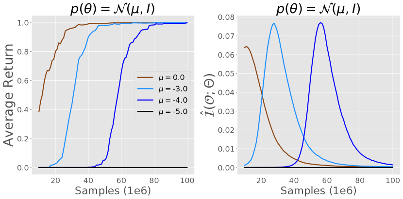
Figure 2: Average return (left) and POIC (right) during the training of evolution strategies. We vary the parameter of initial prior distribution $\mu$ and optimize it. High POIC correctly corresponds to regions of fastest learning.

6 Deep RL Experiments

In this section, we begin by elaborating on how we derive a brute-force task complexity metric to serve as a ground-truth metric to compare with. Then, we study the following questions: (1) Do PIC and POIC metrics correlate well with task complexity across standard deep RL benchmarks such as OpenAI Gym (Brockman et al., 2016; Todorov et al., 2012) and DM Control (Tassa et al., 2018)? (2) Are PIC and POIC more correlated with task complexity than other possible metrics (entropy or variance of returns (Oller et al., 2020))? (3) Can both PIC and POIC be used to evaluate and tune goodness of reward shaping, network architectures, and parameter initialization without requiring running full RL training?

6.1 Defining and Estimating Brute-Force Task Complexity Measure

While an oracle metric for task solvability on complex RL environments seems intractable, one possible (but costly) alternative is to run a large set of diverse RL algorithms and evaluate their normalized average performances. On any given environment, some of these algorithms may completely and efficiently solve the task while others may struggle to learn; an appropriate averaging of the performances of the algorithms can serve as a “ground-truth” task complexity score. As the preparation for the following experiments, we will pre-compute these normalized average performances.

Collecting Raw Algorithm Performances

First, we prepare a bag of algorithms (and hyper-parameters) for learning and execute them all. We treat three types of environments separately; classic control, MuJoCo (Brockman et al., 2016), and DM Control (Tassa et al., 2018). For classic control, we run 23 algorithms, based on PPO (Schulman et al., 2017), DQN (Mnih et al., 2015) and Evolution Strategy with different hyper-parameters for discrete-action, and PPO, DDPG (Lillicrap et al., 2016), SAC (Haarnoja et al., 2018), and Evolution Strategy with different hyper-parameters for continuous-action space environments. For MuJoCo and DM Control, we run SAC, MPO (Abdolmaleki et al., 2018) and AWR (Peng et al., 2019), and to simulate more diverse set of algorithms, we additionally incorporated the leaderboard scores reported in previous SoTA works (Fujimoto et al., 2018; Peng et al., 2019; Laskin et al., 2020). See Appendix C.1 for further details.

Computing Normalized Scores (Algorithm)

After collecting raw performances, we compute the average return over the all algorithms $r_{\text{ave}}^{\text{algo}}$. For the comparison, we need to align the range of reward that is different from each environment. To normalize average return over the environments, we take the maximum between this algorithm-based and random-sampling-based maximum scores (explained below), and use the minimum return obtained by random policy sampling:

$$\text{Normalized Score}:=\frac{r_{\text{ave}}^{\text{algo}}-r_{\min}^{\text{rand}}}{\max(r_{\max}^{\text{rand}},~{}r_{\max}^{\text{algo}})-r_{\min}^{\text{rand}}}.$$

As a sanity check, we checked that the task scores do not trivially correlate with obvious properties of MDP or policy networks, such as state, action dimensionalities; episodic horizon in Appendix C.3.

Computing Normalized Scores (Random Sampling)

In addition to “bag-of-algorithms” task scores, we also compute random-sampling-based task scores that are considered in Oller et al. (2020) for characterizing task difficulties; see Appendix C.2 for more details. While this metric is easier to compute, this only measures the task difficulty of an environment with respect to random search algorithm, and ignores the availability of more advanced RL algorithms.

6.2 Evaluating PIC and POIC as Task Complexity Measures

To verify that our MI-based metrics perform favorably as task solvability metrics in practical settings, we measure both PIC and POIC, along with other alternative metrics, following the random-sampling protocol in Algorithm 1 on the standard RL benchmarks: CartPole, Pendulum, MountainCar, MountainCarContinuous, and Acrobot from classic control in Open AI Gym; HalfCheetah, Walker2d, Humanoid, and Hopper from MuJoCo tasks; cheetah run, reacher easy, and ball_in_cup catch in DM Control (see Appendix A).

We prepare a “bag-of-policy-architectures” to model a realistic prior over policy functions practitioners would use: ([0] layers $+$ [1, 2] layers $\times$ [4, 32, 64] hidden units) $\times$ [Gaussian prior $\mathcal{N}(0,I)$, Uniform prior $\textit{Unif}(-1,1)$, Xavier Normal, Xavier Uniform] $\times$ [w/ bias, w/o bias]; totally 56 variants of architectures. We sample 1,000 parameters from the prior for each architecture, and evaluate each of them with 1,000 episode per parameter ($N=56\times 1000=56000$ and $M=1000$) for random policy sampling. The number of bins for discretization is set to $B=10^{5}$ for surely maximizing PIC. To compare the suitability of our information capacity metrics and Shannon entropy or variance as task solvability metrics, we compute Pearson correlation coefficients between these measures and the normalized scores for the quantitative evaluation.

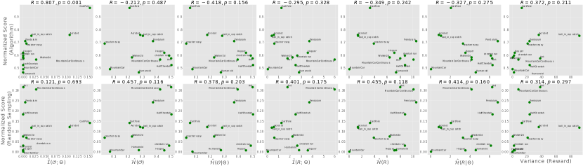
Figure 3: 2D-Scatter plots between each metric (x-axis) and normalized scores (algorithm-based (top) and random-sampling-based (bottom) ; y-axis); see Table 11 for labeled values with environment names. Variance (last column) approximately corresponds to the metric proposed by Oller et al. (2020). POIC ($\hat{\mathcal{I}}(\mathcal{O};\Theta)$) positively correlates with algorithm-based normalized score ($\bf{R=0.807}$; statistically significant with $p<0.01$), the more realistic of the two task difficulty scores, more than all other alternatives including variance of returns (Oller et al., 2020). Note that the two normalized task scores have a low correlation of $0.139$ (see Figure 9), and therefore a high correlation in one means a low correlation in the other.

Figure 3 visualizes the relation between metrics computed via random sampling (Algorithm 1) and normalized scores (see Table 11 in Appendix F for the detailed scores). Note that variance of returns is scaled by $r_{\max}^{\text{rand}}-r_{\min}^{\text{rand}}$ for a normalized comparison among different environments. The results suggest that POIC seems to positively correlate better with algorithm-based normalized score ($R=0.807$; statistically significant with $p<0.01$) compared to any other alternatives, such as reward marginal entropy ($R=-0.349$) or variance of returns ($R=0.372$) (Oller et al., 2020). Here, we can see that POIC seems to work as a task solvability metric in standard RL benchmarks. In contrast, PIC is correlated with random-sampling-based normalized score ($R=0.401$) and superior to variance of returns ($R=0.314$). However, it is less correlated with algorithm-based task scores, which seems closer to actual task difficulty. These differences are possibly due to maximization bias in optimality variable from exponential transform and estimation in Bernoulli space.

6.3 Evaluating the Goodness of Reward Shaping and Other “Hyper-Parameters” without RL

We additionally test whether both PIC and POIC can directly evaluate the goodness of reward shaping properly. We investigate two goal-oriented tasks, Reacher (Todorov et al., 2012) and Pointmaze (Fu et al., 2020), where both tasks are defined based on distance functions. We prepare the following four families of distance reward functions: L1 norm, L2 norm, Fraction, and Sparse, each with 1 or 2 hyper-parameters. We select 4 hyper-parameter values for each, totaling 16 different reward functions. To get the normalized scores, we run PPO with 500k steps and 5 seeds for each (see Appendix G for the details).

Figure 4 reveals that Pearson correlation coefficients between the normalized score and information capacity metrics have positive correlations (statistically significant with $p<0.05$). Coincidentally, clustering of L1 and L2 results reveals that these two reward families are much more robust to ill-specified reward hyper-parameters (i.e. require much less hyper-parameter tuning) than Fraction and Sparse, which is expected given the smoothness and low curvatures of L1 and L2. The results show that both PIC and POIC can evaluate the goodness of reward shaping for optimizability. We run additional experiments to evaluate the goodness of architectures, initializations, and dynamics noises. See Appendix H and J for the details.

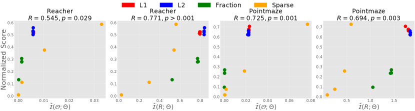
Figure 4: 2D-Scatter plots between PIC or POIC (x-axis) and normalized score (y-axis), after 500k training steps and averaged with 5 seeds. We test 4 family of reward functions (L1 norm, L2 norm, Fraction, Sparse) and 4 variants each (see Appendix G for the details). The results indicate that both PIC and POIC can be used to evaluate the goodness of reward shaping proposals. The clusterings of L1 and L2 rewards indicate that learning difficulty with those reward functions does not vary much with hyper-parameters, and suggest that they do not require much hyper-parameter tuning in practice for these tasks.

7 Limitation and Future Work

We tackle a seemingly intractable problem: to quantify the difficulty of an RL environment irrespective of learning algorithms. While our empirical evaluations present many encouraging positive results, our metrics have obvious limitations. The biggest is the dependence on $p(\theta)$. As discussed in Section 5, $p(\theta)$ intuitively defines an effective search area (in function space or function parameter space) and our two information capacity metrics approximately measure the easiness of searchability and maximizability respectively within this area weighted by a prior search distribution. Since these metrics in our experiments are only measured at initialization (except results in Figure 2 and Appendix B), they may not correspond well with overall task solvability: (1) if the optimization landscape drastically changes in the later stages of learning, particularly likely for neural networks (Li et al., 2017) or MDPs with discontinuous rewards or dynamics; or (2) if $p(\theta)$ poorly approximates actual search directions given by SGD, natural gradients, Q-learning, etc., during learning. Exploring our metrics throughout the dynamics of optimization and learning to adapt $p(\theta)$ are some of the exciting future directions, along with making connections to works in supervised learning that relate convergence to signal-to-noise ratios in gradient estimators (Saxe et al., 2019; Smith et al., 2017; Smith & Le, 2017). Another important direction is to scale the evaluations to problems requiring larger neural networks, like ALE with image observations (Bellemare et al., 2013).

8 Conclusion

We defined policy information capacity (PIC) and policy-optimal information capacity (POIC) as information-theoretic metrics for numerically analyzing the generic task complexities of RL environments. These metrics are simple and practical: estimating these metrics only requires a prior distribution over policy functions $p(\theta)$ and trajectory sampling. We formalized a quantitative evaluation protocol for verifying the correctness of task difficulty metrics, that properly accounts for both the richness of available RL algorithms and the complexities of high-dimensional benchmark environments. Through careful experimentation, we successfully identified POIC as the only metric that exhibited high correlations with a brute-force measurement of environment complexity, and demonstrated that these PIC and POIC metrics can be used for tuning task parameters such as reward shaping, MDP dynamics, network architecture and initialization for best learnability without running RL experiments. We hope our work can inspire future research to further explore these long overdue questions of analyzing, measuring, and categorizing the properties of RL environments, which can guide us to developing even better learning algorithms.

Appendix

Appendix A Details of Environments

In this section, we explain the details of the environments used in our experiments. The properties of each environment are summarized in Table 2.

Environment	State dim	Action dim	Control	Episode Length
CartPole-v0	4	2	Discrete	200
Pendulum-v0	3	1	Continuous	200
MountainCar-v0	2	3	Discrete	200
MountainCarContinuous-v0	2	1	Continuous	999
Acrobot-v1	6	3	Discrete	500
Ant-v2	111	8	Continuous	1000
HalfCheetah-v2	17	6	Continuous	1000
Hopper-v2	11	3	Continuous	1000
Walker2d-v2	17	6	Continuous	1000
Humanoid-v2	376	17	Continuous	1000
cheetah run	17	6	Continuous	1000
reacher easy	6	2	Continuous	1000
ball_in_cup catch	8	2	Continuous	1000
Reacher	11	2	Continuous	50
Pointmaze	4	2	Continuous	150

Table 2: The details of Open AI Gym and DeepMind Control Suite Environments used in this paper.

CartPole

The states of CartPole environment are composed of 4-dimension real values, cart position, cart velocity, pole angle, and pole angular velocity. The initial states are uniformly randomized. The action space is discretized into 2-dimension. The cumulative reward corresponds to the time steps in which the pole isn’t fallen down.

Pendulum

The states of Pendulum environment are composed of 3-dimension real values, cosine of pendulum angle $\cos{\varphi}$, sine of pendulum angle $\sin{\varphi}$, and pendulum angular velocity $\dot{\varphi}$. The initial states are uniformly randomized. The action space is continuous and 1-dimension. The reward is calculated by the following equation;

$$r_{t}=-(\varphi_{t}^{2}+0.1*\dot{\varphi_{t}}^{2}+0.001*\|\bm{a}_{t}\|_{2}^{2}).$$

MountainCar

The states of MountainCar environment are composed of 2-dimension real values, car position, and its velocity. The initial states are uniformly randomized. The action space is discretized into 3-dimension. The cumulative reward corresponds to a negative value of the time steps in which the car doesn’t reach the goal region.

MountainCarContinuous

The 1-dimensional continuous action space version of MountainCar environment. The reward is calculated by the following equation;

$$r_{t}=-0.1*\|\bm{a}_{t}\|_{2}^{2}+100*\mathbbm{1}[x_{t}\geq x_{g}~{}\text{and}~{}\dot{x}_{t}\geq\dot{x}_{g}].$$

Acrobot

The states of Acrobot environment consist of 6-dimension real values, sine, and cosine of the two rotational joint angles and the joint angular velocities. The initial states are uniformly randomized. The action space is continuous and 3-dimension. The cumulative reward corresponds to a negative value of the time steps in which the end-effector isn’t swung up at a height at least the length of one link above the base.

Ant

The state space is 111-dimension, position and velocity of each joint, and contact forces. The initial states are uniformly randomized. The action is an 8-dimensional continuous space. The reward is calculated by the following equation;

$$r_{t}=\dot{x}_{t}-0.5*\|\bm{a}_{t}\|_{2}^{2}-0.0005*\|\bm{s}_{t}^{\text{contact}}\|_{2}^{2}+1.$$

HalfCheetah

The state space is 17-dimension, position and velocity of each joint. The initial states are uniformly randomized. The action is a 6-dimensional continuous space. The reward is calculated by the following equation;

$$r_{t}=\dot{x}_{t}-0.1*\|\bm{a}_{t}\|_{2}^{2}.$$

Hopper

The state space is 11-dimension, position and velocity of each joint. The initial states are uniformly randomized. The action is a 3-dimensional continuous space. This environment is terminated when the agent falls down. The reward is calculated by the following equation;

$$r_{t}=\dot{x}_{t}-0.01*\|\bm{a}_{t}\|_{2}^{2}+1.$$

Walker2d

The state space is 17-dimension, position and velocity of each joint. The initial states are uniformly randomized. The action is a 6-dimensional continuous space. This environment is terminated when the agent falls down. The reward is calculated by the following equation;

$$r_{t}=\dot{x}_{t}-0.01*\|\bm{a}_{t}\|_{2}^{2}+1.$$

Humanoid

The state space is 376-dimension, position and velocity of each joint, contact forces, and friction of actuator. The initial states are uniformly randomized. The action is a 17-dimensional continuous space. This environment is terminated when the agent falls down. The reward is calculated by the following equation;

$$r_{t}=1.25*\dot{x}_{t}-0.1*\|\bm{a}_{t}\|_{2}^{2}-\min(5e^{-7}*\|\bm{s}_{t}^{\text{contact}}\|_{2}^{2},~{}10)+5.$$

cheetah run

The state space is 17-dimension, position and velocity of each joint. The initial states are uniformly randomized. The action is a 6-dimensional continuous space. The reward is calculated by the following equation;

$$r_{t}=\begin{cases}0.1*\dot{x}_{t}&(0\leq\dot{x}_{t}\leq 10)\\ 1&(\dot{x}_{t}>10).\end{cases}$$

reacher easy

The state space is 6-dimension, position and velocity of each joint. The initial states are uniformly randomized. The action is a 2-dimensional continuous space. The reward is calculated by the following equation;

$$r_{t}=\mathbbm{1}[x_{t}-x_{g}\leq\epsilon].$$

ball_in_cup catch

The state space is 8-dimension, position and velocity of each joint. The initial states are uniformly randomized. The action is a 2-dimensional continuous space. The reward is calculated by the following equation;

$$r_{t}=\mathbbm{1}[x_{t}-x_{g}\leq\epsilon].$$

Reacher

The state space is 11-dimension, position and velocity of each joint. The initial states are uniformly randomized. The action is a 2-dimensional continuous space. We modify the reward function for the experiments (see Appendix G).

Pointmaze

We use the implementation provided by Fu et al. (2020) (Figure 12). The state space is 4-dimension, position and velocity. The initial states are uniformly randomized. The action is a 2-dimensional continuous space. We modify the reward function for the experiments (see Appendix G).

Appendix B Additional Details of Synthetic Experiments

We provide the rest of the results, presented in Section 5, and then show additional comparisons between PIC or POIC and marginal entropies in this setting.

B.1 Answer to (2) in Section 5

First, Figure 5 shows the full results of Figure 2, which holds the same tendency overall.

Similar to the results of POIC, presented in Section 5, we also investigate what happens to PIC throughout a realistic learning process, optimizing $\mu$ in $p(\theta)$ to solve the MDP by evolution strategy and observing this metric and performance of the agent during training. Following the experimental settings of POIC, we assume the Gaussian prior, $\mathcal{N}(\mu,I)$, and vary $\mu$ initializations using $[-10,-5,-4,-3,-2,-1,0,1,2,3,4,5,10]$. We set $N=M=1000$, and horizon is $T=3$. Figure 6 reveals that the initial prior with high PIC (e.g. $\mu=0$) actually solves the environment faster than those with low PIC (e.g. $\mu=-3.0,-4.0,-5.0$), which seems the same as the case of POIC. Interestingly, Figure 6 also shows that high PIC corresponds to regions of fastest learning.

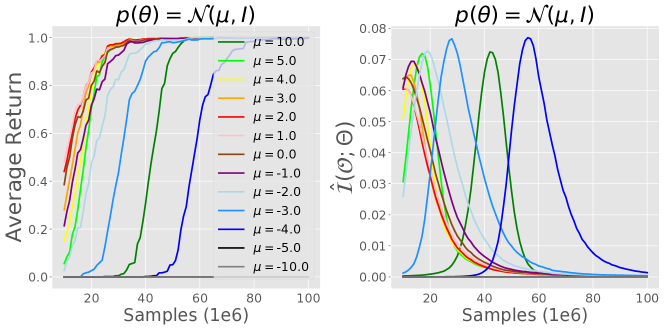
Figure 5: Average return (left) and POIC (right) during the training of evolution strategies. We change the parameter of initial prior distribution $\mu$ and optimize it.

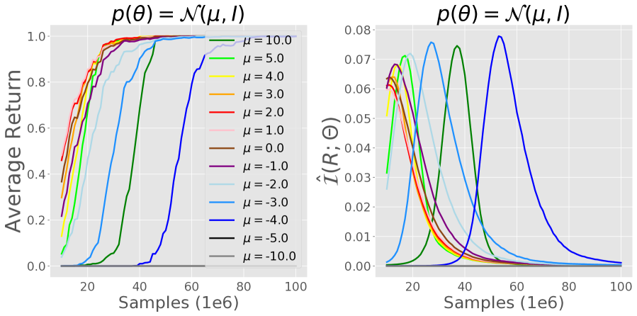
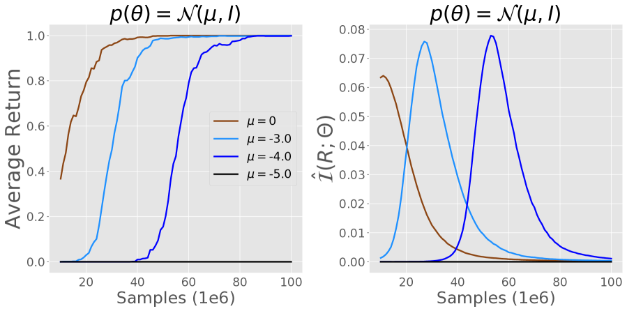
(a) All results (b) $\mu=0.0,-3.0,-4.0,-5.0$

Figure 6: Average return and PIC during the training of evolution strategies. We vary the parameter of initial prior distribution $\mu$ and optimize it. (a) shows the all results, and in (b), we extract a few of them ($\mu=0.0,-3.0,-4.0,-5.0$; we separate these for the visibility). High PIC surely corresponds to regions of faster learning, which is similar trends of POIC.

B.2 Are PIC and POIC more suitable for evaluating task solvability than other alternatives?

We consider the relations between the normalized score and each reward-based metric ($\mathcal{I}(R;\Theta)$, $\mathcal{H}(R)$, $\mathcal{H}(R|\Theta)$), or optimality-based metric ($\mathcal{I}(\mathcal{O};\Theta)$, $\mathcal{H}(\mathcal{O})$, $\mathcal{H}(\mathcal{O}|\Theta)$) on the MDP $\mathcal{M}$, for a variety of the prior distributions. We test two variants of Gaussian prior, (a) $\mathcal{N}(\mu,I)$ (changing $\mu\in\{-10,-5,-4,-3,-2,-1,0,1,2,3,4,5,10\}$), and (b) $\mathcal{N}(0,\sigma^{2}I)$ (changing $\sigma\in\{0.1,0.2,...,0.9,1.0\}$). We set $N=M=1000$, and the horizon is $T=3$ (note that as far as we observed, $N=M=100$ could not estimate POIC metric properly). Figure 7 indicates the relation between each metric of reward and normalized score. In (a), we change $\mu$, and in (b) we change $\sigma$. We see that PIC shows positive correlation to normalized score both in (a) ($R=0.95$) and (b) ($R=0.78$). The marginal and conditional entropies show, however, positive correlation in (a) (both $R=0.99$), but negative in (b) ($R=-0.83$ and $R=-0.80$). This suggests that there are cases where the marginal or conditional entropy alone might not reflect task solvability appropriately. Similar to PIC, we see in Figure 8 that POIC shows positive correlation to normalized score both in (a) ($R=0.94$) and (b) ($R=0.69$). The marginal and conditional entropies show, however, positive correlation in (a) (both $R=0.99$), but negative in (b) ($R=-0.82$ and $R=-0.72$).

These observations suggest that there are cases where the marginal or conditional entropy alone might not reflect task solvability appropriately.

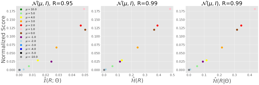
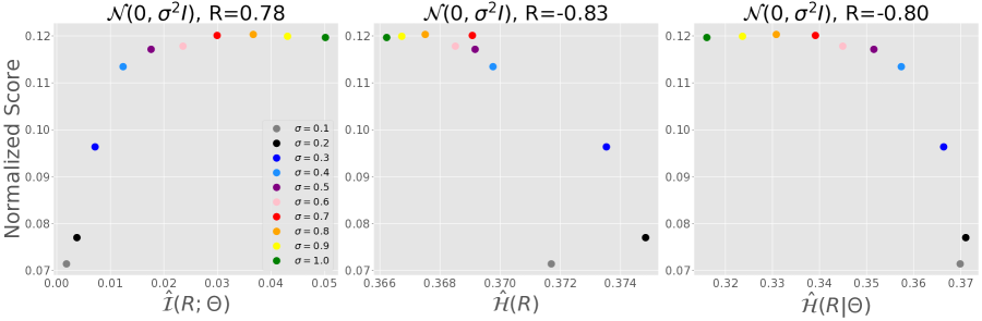
(a) $p(\theta)=\mathcal{N}(\mu,I)$ (b) $p(\theta)=\mathcal{N}(0,\sigma^{2}I)$

Figure 7: Relation between each metric (x-axis; PIC (left), marginal entropy (middle), conditional entropy (right)) and normalized score (y-axis). We compute the Pearson correlation coefficient (above the plots). In (a), we change $\mu$, and in (b) we change $\sigma$. PIC is the only metric that shows a consistently positive correlation. The marginal and conditional entropy doesn’t have such consistency.

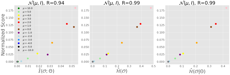
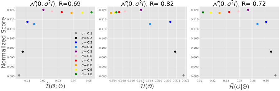
(a) $p(\theta)=\mathcal{N}(\mu,I)$ (b) $p(\theta)=\mathcal{N}(0,\sigma^{2}I)$

Figure 8: Relation between each metric (x-axis; POIC (left), marginal entropy (middle), conditional entropy (right)) and normalized score (y-axis). We compute the Pearson correlation coefficient (above the plots). In (a), we change $\mu$, and in (b) we change $\sigma$. Same as the case of PIC (Figure 7), POIC is the only metric that shows a consistently positive correlation. The marginal and conditional entropy doesn’t have such consistency.

Appendix C Normalized Score as Task Complexity Measure

In this section, we explain the details of normalized score. One intuitive and brute-force approach to measure the ground-truth task complexity in complex environments is to compare the performances of just an average agent among the environments. When we try to realize this impractical method, we face two difficulties: (1) how can we obtain an average agent? (2) how do we manage the different reward scale among the different environments?

To deal with (1), we have two options: substituting average score among diverse RL algorithms or random policy sampling score, for the performance of average agent. We can also solve (2) by normalizing some average quantity divided by max-min value. In the following section, we explain the details of each approach.

C.1 Algorithm-based Normalized Score

To compute the normalized score, we prepare the set of algorithms for evaluation and then execute them all. Since algorithms with different hyper-parameter behave differently, we treat them as different “algorithms”. After the evaluation, we compute the average return over the algorithms $r_{\text{ave}}^{\text{algo}}$. This value, however, completely differs from all environments, due to the range of reward. To normalize average return for the comparison over the environments, we compute the maximum return $r_{\max}$ and minimum return $r_{\min}$. In practice, we take the maximum between this algorithm-based and random-sampling-based maximum scores, and use the minimum return obtained by random policy sampling:

$$\text{Normalized Score}=\frac{r_{\text{ave}}^{\text{algo}}-r_{\min}^{\text{rand}}}{\max(r_{\max}^{\text{rand}},~{}r_{\max}^{\text{algo}})-r_{\min}^{\text{rand}}}.$$

We use three types of environments, classic control, MuJoCo, and DeepMind Control Suite (DM Control). For MuJoCo and DM Control, we test SAC, MPO and AWR. To simulate the diverse set of algorithms, we employ the leaderboard scores reported in previous SoTA works (Fujimoto et al., 2018; Peng et al., 2019; Laskin et al., 2020).

C.1.1 Classic Control

For classic control, we run 23 algorithms, based on PPO, DQN and Evolution Strategy for discrete action space environments, and PPO, DDPG, SAC, and Evolution Strategy for continuous action space environments with different hyper-parameters, such as network architecture or discount factor (Table 3). We average each performance with 5 random seeds, and also average over algorithms.

C.1.2 MuJoCo

We test SAC, MPO and AWR, following hyper parameters in original implementations. We average each performance with 10 random seeds and train each agent 1M steps for Hopper, 3M for Ant, HalfCheetah, Walker2d, and 10M for Humanoid (Table 5). To simulate the diverse set of algorithms, we employ the leaderboard scores reported in previous works (Fujimoto et al., 2018; Peng et al., 2019) (Table 6 and Table 7). Totally, we use 17 algorithms for Ant, HalfCheetah, Hopper and Walker2d, and 10 algorithms for Humanoid to compute $r_{\text{ave}}^{\text{algo}}$ and $r_{\max}^{\text{algo}}$ (Table 4).

C.1.3 DeepMind Control Suite

We also test SAC, MPO and AWR, following hyper parameters in original implementations (Table 9). We average each performance with 10 random seeds and train each agent 500k steps. To simulate the diverse set of algorithms, we employ the leaderboard scores reported in previous work (Laskin et al., 2020) (Table 10). Totally, we use 11 algorithms for cheetah run and ball_in_cup catch, and 10 algorithms for reacher easy to compute $r_{\text{ave}}^{\text{algo}}$ and $r_{\max}^{\text{algo}}$ (Table 8).

C.2 Random-Sampling-based Normalized Score

In Oller et al. (2020), they compute some representatives (e.g. 99.9 percentile score) obtained via random weight guessing and compare them qualitatively among the variety of environments. We extend this idea to our settings – quantitative comparison of the task difficulty.

Through the random policy sampling, we can compute the average cumulative reward $r_{\text{ave}}^{\text{rand}}$ and then normalize it using maximum return $r_{\max}$ and minimum return $r_{\min}$. In practice, we take the maximum between this algorithm-based and random-search-based maximum scores, and use the minimum return obtained by random policy search:

$$\text{Normalized Score}:=\frac{r_{\text{ave}}^{\text{rand}}-r_{\min}^{\text{rand}}}{\max(r_{\max}^{\text{rand}},~{}r_{\max}^{\text{algo}})-r_{\min}^{\text{rand}}}.$$

This method seems easy to use since we do not need extensive evaluations by a variety of RL algorithms. However, this random-sampling-based normalized score is highly biased towards the early stage of learning. It might not reflect the overall nature of environments properly.

C.3 Correlation to Obvious Properties of MDP

In this section, we verify that these brute-force task solvability metrics do not just depend on obvious properties of MDP or policy networks, such as state and action dimensionalities, horizon, and the other type of normalized score.

Figure 9 summarizes the correlation among those metrics. While some properties such as action dimensions or episode length have negative correlations with algorithm-based normalized score, compared to Figure 3, our proposed POIC seems much better than those metrics (see also Table 11 for the details).

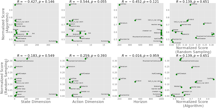
Figure 9: 2D-Scatter plots between each metric (State dimension, action dimension, episode horizon, and normalized scores; x-axis) and each normalized score (algorithm-based (top) and random-sampling-based (bottom); y-axis).

Algorithm	Hyper-Parameters	CartPole	Pendulum	MountainCar	MountainCarContinuous	Acrobot
PPO	(64, 64), $\gamma=0.995$	200.00	-1045.16	-97.48	65.05	-66.84
PPO	(64, 64), $\gamma=0.99$	200.00	-582.53	-117.83	18.82	-67.15
PPO	(64, 64), $\gamma=0.95$	200.00	-170.45	-158.77	9.53	-67.42
PPO	(128, 64), $\gamma=0.995$	200.00	-1152.09	-118.02	95.89	-67.42
PPO	(128, 64), $\gamma=0.99$	200.00	-467.42	-104.73	0.00	-72.83
PPO	(128, 64), $\gamma=0.95$	199.75	-151.43	-116.44	0.00	-68.09
PPO	(128, 128), $\gamma=0.995$	200.00	-1143.59	-97.22	56.81	-64.83
PPO	(128, 128), $\gamma=0.99$	200.00	-707.25	-97.21	30.75	-64.90
PPO	(128, 128), $\gamma=0.95$	199.79	-161.28	-98.82	0.00	-67.25
ES	(16, 16), $\sigma=0.1$	200.00	-1062.54	-128.82	0.00	-80.30
ES	(16, 16), $\sigma=0.1$, rand	200.00	-1059.30	-127.67	0.00	-79.57
ES	(16, 16), $\sigma=0.3$, rand	143.19	-1175.70	-200.00	0.00	-182.21
ES	(64, 64), $\sigma=0.1$	200.00	-999.26	-136.48	0.00	-80.97
ES	(64, 64), $\sigma=0.1$, rand	200.00	-1012.32	-131.85	0.00	-80.83
ES	(64, 64), $\sigma=0.3$, rand	158.43	-1180.50	-200.00	0.00	-257.48
DQN	(100, 100), $\gamma=0.95$	188.80	–	-200.00	–	-360.57
DQN	(100, 100), $\gamma=0.99$	200.00	–	-164.76	–	-250.53
DQN	(200, 200), $\gamma=0.95$	176.69	–	-192.70	–	-296.48
DQN	(200, 200), $\gamma=0.99$	200.00	–	-150.86	–	-381.99
DQN	(50, 50), $\gamma=0.95$	200.00	–	-154.91	–	-318.57
DQN	(50, 50), $\gamma=0.99$	200.00	–	-167.02	–	-329.15
DQN	(50, 50, 50), $\gamma=0.95$	200.00	–	-167.91	–	-274.28
DQN	(50, 50, 50), $\gamma=0.99$	200.00	–	-167.22	–	-169.92
SAC	(128, 128), $\gamma=0.99$	–	-129.30	–	0.00	–
SAC	(128, 128), $\gamma=0.95$	–	-138.26	–	0.00	–
SAC	(256, 256), $\gamma=0.99$	–	-128.63	–	0.00	–
SAC	(256, 256), $\gamma=0.95$	–	-138.27	–	19.21	–
DDPG	(150, 50), $\gamma=0.95$	–	-138.76	–	0.00	–
DDPG	(150, 50), $\gamma=0.99$	–	-130.35	–	0.00	–
DDPG	(400, 300), $\gamma=0.95$	–	-138.61	–	0.00	–
DDPG	(400, 300), $\gamma=0.99$	–	-131.21	–	0.00	–
$r_{\text{ave}}^{\text{algo}}$	–	194.20	-571.49	-143.12	12.87	-162.92
$r_{\max}^{\text{algo}}$	–	200.00	-128.63	-97.21	95.89	-64.83

Table 3: Performance of a variety of algorithms in classic control. The results are averaged over 5 random seeds. We change 2 hyper-parameters, architecture of neural networks and discount factor $\gamma$.

Environments	Average	Maximum
Ant	2450.8	6584.2
HalfCheetah	6047.2	15266.5
Hopper	2206.7	3564.1
Walker2d	3190.8	5813.0
Humanoid	3880.8	8264.0

Table 4: Average and maximum scores in MuJoCo environments, calculated from 17 algorithms (10 for Humanoid) (Table 5, Table 6 and Table 7).

Environments	SAC	MPO	AWR
Ant	5526.4	6584.2	1126.7
HalfCheetah	15266.5	11769.6	5742.4
Hopper	2948.9	2135.5	3084.7
Walker2d	5771.8	3971.5	4716.6
Humanoid	8264.0	5708.7	5572.6

Table 5: SAC, MPO and AWR results in MuJoCo environments. These results are averaged across 10 seeds.

Environments	TRPO	PPO	DDPG	TD3	SAC	RWR	AWR
Ant	2901	1161	72	4285	5909	181	5067
HalfCheetah	3302	4920	10563	4309	9297	1400	9136
Hopper	1880	1391	855	935	2769	605	3405
Walker2d	2765	2617	401	4212	5805	406	5813
Humanoid	552	695	4382	81	8048	509	4996

Table 6: Performance of a variety of algorithms in MuJoCo environments, reported by Peng et al. (2019). These results are averaged across 5 seeds.

Environments	TD3	DDPG(1)	DDPG(2)	PPO	TRPO	ACKTR	SAC
Ant	4372	1005	889	1083	-76	1822	655
HalfCheetah	9637	3306	8577	1795	-16	1450	2347
Hopper	3564	2020	1860	2165	2471	2428	2997
Walker2d	4683	1844	3098	3318	2321	1217	1284

Table 7: Performance of a variety of algorithms in MuJoCo environments, reported by Fujimoto et al. (2018) after 1M steps. These results are averaged across 10 seeds.

Environments	Average	Maximum
cheetah run	474.4	795.0
reacher easy	691.5	961.2
ball_in_cup catch	751.7	978.2

Table 8: Average and maximum scores in DM Control environments, calculated from 11 algorithms (10 for reacher easy) (Table 9 and Table 10).

Environments	SAC	MPO	AWR
cheetah run	536.0	253.9	125.2
reacher easy	961.2	841.5	530.2
ball_in_cup catch	971.9	957.3	135.2

Table 9: SAC, MPO and AWR results in DM Control environments after 500k steps. These results are averaged across 10 seeds.

Environments	RAD	CURL	PlaNet	Dreamer	SAC+AE	SLACv1	Pixel SAC	State SAC
cheetah run	728	518	305	570	550	640	197	795
reacher easy	955	929	210	793	627	–	145	923
ball_in_cup catch	974	959	460	879	794	852	312	974

Table 10: Performance of a variety of algorithms in DM Control environments, reported by Laskin et al. (2020), after 500k training steps. These results are averaged across 10 seeds.

Appendix D Policy and Policy-Optimal Information Capacity during ES Training

We evaluate how PIC and POIC behave during RL training (reward maximization) on complex benchmarking environments, in contrast to synthetic ones in Section 5. We train linear, (4, 4) and (16, 16) neural networks with evolution strategy (ES) (Salimans et al., 2017). 100 parameters are sampled from the trainable prior distribution $p_{\mu}(\theta)=\mathcal{N}(\mu,\sigma=0.1)$ (ES optimizes $\mu$) in each epoch, and the agent runs 100 episodes per parameters to calculate both PIC and POIC. Section 10 shows the learning curves (top row), corresponding POIC $\mathcal{I}(\mathcal{O};\Theta)$ (middle) and PIC $\mathcal{I}(R;\Theta)$ (bottom). As we observed in Section 5, both information capacity metrics increase during training, and after each performance converges, they gradually decrease. It might be related to higher correlation of POIC to algorithm-based normalized score shown in Section 6 that POIC seems to follow these trends better than PIC (e.g. Pendulum and HalfCheetah).

Another interesting observation of POIC can be seen in HalfCheetah, where (4, 4) network (green; top) converges to sub-optimal solution and (16, 16) network (blue; top) gets away from there. The agents that can have multi-modal solutions keeps high POIC (green; middle) after sub-optimal convergence, while POIC decreases as improving performance (blue; middle). This might suggests that a sub-optimal prior distribution $p_{\mu}(\theta)=\mathcal{N}(\mu,\sigma=0.1)$ still can be easy to minimize the rewards (green), though the further improvements (blue) make it lean towards maximization (i.e. less controllable). Measuring PIC and POIC with more familiar on-policy algorithms such as PPO or TRPO remains as future work.

Figure 10: The average returns (top), POIC (middle) and PIC (bottom) during ES training. We use several classic control and MuJoCo tasks. Both information capacity metrics increase during training, and after each performance converges, they gradually decrease. It might be related to higher correlation of POIC to algorithm-based normalized score shown in Section 6 that POIC seems to follow these trends better than PIC (e.g. Pendulum and HalfCheetah).

Appendix E A Proof of Proposition 1

Assume that $\theta_{1}$ is better than $\theta_{2}$ without loss of generality.

The proof relies on the following Chernoff’s bound tailored for a normal distribution (Boucheron et al., 2013): for $N$ independent samples $(X_{n})_{n=1,\ldots,N}$ from a normal distribution $\mathcal{N}(\mu,\sigma^{2})$, and $\mu$’s $N$-sample-estimate $\hat{\mu}:=\sum_{n=1}^{N}X_{n}/N$,

$$\Pr\left\{\hat{\mu}\leq\mu-\varepsilon\right\}\leq\exp\left(-\frac{N\varepsilon^{2}}{2\sigma^{2}}\right)$$

holds. Applying this bound to our case with $\hat{\mu}=\hat{\mu}_{1}-\hat{\mu}_{2}$, $\mu=\mu_{\theta_{1}}-\mu_{\theta_{2}}$, and $\varepsilon=\mu$, we obtain

$$\Pr\left\{\hat{\mu}_{1}-\hat{\mu}_{2}\leq 0\middle|\theta_{1},\theta_{2}\right\}\leq\exp\left(-\frac{N}{2}\left(\frac{\mu_{\theta_{1}}-\mu_{\theta_{2}}}{\sigma_{\theta_{1}}+\sigma_{\theta_{2}}}\right)^{2}\right).$$

Since the entropy of $\mathcal{N}(\mu_{\theta},\sigma_{\theta}^{2})$ is $\log(\sigma_{\theta}\sqrt{2\pi e})$, the upper bound can be rewritten as

$$\Pr\left\{\hat{\mu}_{1}-\hat{\mu}_{2}\leq 0\middle|\theta_{1},\theta_{2}\right\}\leq\exp\left(-\pi eN\left(\frac{\mu_{\theta_{1}}-\mu_{\theta_{2}}}{\exp(\mathcal{H}_{1})+\exp(\mathcal{H}_{2})}\right)^{2}\right).$$

Taking the expectation of both sides with respect to $\theta_{1}$ and $\theta_{2}$, the proof is concluded.

Appendix F Full Results on Deep RL Experiment

In this section, we provide the the full results on the experiment in Section 6.2.

We used max 40 CPUs for the experiments in Section 6.2 and it took about at most 2 hours per each random sampling (e.g. HalfCheetah-v2). For estimating brute-force normalized score (Section 6.1 and Appendix C), we mainly used 4 GPUs (NVIDIA V100; 16GB) and it took about 4 hours per seed.

Correlation of Policy-Optimal Information Capacity

As seen in Figure 3, the relation between POIC and the algorithm-based normalized score might seem a bit concentrated or skewed with some outliers. To check the validity of correlation, we remove these outliers and recompute the correlation. Figure 11 exhibits the strong positive correlation still holds ($R=0.780$, statistically significant with $p<0.01$.) after we remove top-3 outliers of POIC (CartPole, Acrobot, and MountainCarContinuous).

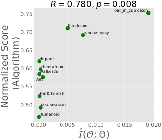
Figure 11: The correlation between POIC and the algorithm-based normalized score. The strong positive correlation still holds ($R=0.780$, statistically significant with $p<0.01$.) after we remove top-3 outliers of POIC (CartPole, Acrobot, and MountainCarContinuous).

Environment	Score(A)	Score(R)	$\hat{\mathcal{I}}(\mathcal{O};\Theta)$	$\hat{\mathcal{H}}(\mathcal{O})$	$\hat{\mathcal{H}}(\mathcal{O}|\Theta)$	$\hat{\mathcal{I}}(R;\Theta)$	$\hat{\mathcal{H}}(R)$	$\hat{\mathcal{H}}(R|\Theta)$	Variance	State dim	Action dim	Horizon
CartPole	0.970	0.141	0.153418	0.210	0.056	1.227	3.262	2.035	12.610	4	2	200
Pendulum	0.710	0.242	0.005060	0.374	0.369	3.708	10.520	6.812	23.223	3	1	200
MountainCar	0.491	0.001	0.000357	0.073	0.073	0.019	0.027	0.008	0.054	2	3	200
MountainCarContinuous	0.566	0.305	0.030092	0.424	0.394	5.953	10.095	4.142	8.022	2	1	999
Acrobot	0.759	0.121	0.106989	0.285	0.178	0.551	1.355	0.803	35.891	6	3	500
Ant	0.575	0.316	0.000751	0.501	0.500	1.767	8.010	6.243	37.830	111	8	1000
HalfCheetah	0.523	0.183	0.000165	0.503	0.503	2.488	8.764	6.276	23.468	17	6	1000
Hopper	0.619	0.007	0.000107	0.453	0.453	3.572	7.088	3.516	3.006	11	3	1000
Walker2d	0.583	0.075	0.000102	0.227	0.227	2.211	6.350	4.139	0.403	17	6	1000
Humanoid	0.466	0.008	5e-05	0.275	0.275	2.792	7.359	4.567	1.917	376	17	1000
cheetah run	0.597	0.030	0.000308	0.487	0.487	2.635	8.743	6.108	1.972	17	6	1000
reacher easy	0.691	0.069	0.007751	0.036	0.029	0.594	3.863	3.268	20.669	6	2	1000
ball_in_cup catch	0.752	0.118	0.019111	0.303	0.284	0.367	1.391	1.024	91.454	8	2	1000
Correlation Coefficient: Score(A)	–	0.139	0.807	-0.212	-0.418	-0.295	-0.349	-0.327	0.372	-0.427	-0.544	-0.452
p-Value: Score(A)	–	0.651	0.001	0.487	0.156	0.328	0.242	0.275	0.211	0.146	0.055	0.121
Correlation Coefficient: Score(R)	0.139	–	0.121	0.457	0.378	0.401	0.455	0.414	0.314	-0.183	-0.259	-0.016
p-Value: Score(R)	0.651	–	0.693	0.116	0.203	0.175	0.118	0.160	0.297	0.549	0.393	0.959

Table 11: The raw results of POIC $\hat{\mathcal{I}}(\mathcal{O};\Theta)$, optimality marginal entropy $\hat{\mathcal{H}}(\mathcal{O})$, optimality conditional entropy $\hat{\mathcal{H}}(\mathcal{O}|\Theta)$, PIC $\hat{\mathcal{I}}(R;\Theta)$, reward marginal entropy $\hat{\mathcal{H}}(R)$, reward conditional entropy $\hat{\mathcal{H}}(R|\Theta)$, normalized variance of return in standard RL benchmark environments, Pearson correlation coefficient to the algorithm-based normalized score (Score(A)), and the random-sampling-based normalized score (Score(R)). We prepare bags of policy architectures, totally 56 variants of architectures; ([0] layers $+$ [1, 2] layers $\times$ [4, 32, 64] units) $\times$ [Gaussian prior $\mathcal{N}(0,I)$, Uniform prior $\textit{Unif}(-1,1)$, Xavier Normal, Xavier Uniform] $\times$ [w/ bias, w/o bias]. The results suggest that POIC seems to positively correlate well with algorithm-based normalized score better than any other alternatives, such as marginal reward entropy or variance of returns (Oller et al., 2020).

Appendix G Details of Reward Shaping Experiments

Here, we present hyper-parameters of the reward functions and raw experimental results (Table 12 for Reacher and Table 13 for Pointmaze (Figure 12)). In the experiment, we employ the following four families of goal-oriented reward function:

1. L1 norm: $r(s,s_{g})=-\alpha\|s-s_{g}\|_{1}$,

2. L2 norm: $r(s,s_{g})=-\alpha\|s-s_{g}\|_{2}$,

3. Fraction: $r(s,s_{g})=\frac{\beta}{\gamma+\|s-s_{g}\|_{2}}$,

4. Sparse: $r(s,s_{g})=-\mathbbm{1}[\|s-s_{g}\|_{2}\geq\epsilon]$.

This notations of hyper-parameter correspond to Table 12 and Table 13. To estimate information capacity metrics, we use the small neural networks (2 layers, 4 hidden units, Gaussian initialization $\mathcal{N}(0,I)$, and without bias term) for the simplicity. For the following RL training, we employ the same policy architectures, while keeping original value networks sizes (2 layers, 64 hidden units). We normalize the scores of PPO, trained 500 steps and averaged among 5 seeds for fair comparisons among different reward-scale environments.

Reward	Hyper-parameter	$r_{\max}^{\text{rand}}$	PPO (500k)	Normalized Score	$\hat{\mathcal{I}}(R;\Theta)$	$\hat{\mathcal{I}}(\mathcal{O};\Theta)$
L1-norm	$\alpha=1.0$	-0.557	-8.776	0.507	0.796	5.801e-3
L1-norm	$\alpha=0.5$	-0.316	-4.245	0.524	0.798	5.785e-3
L1-norm	$\alpha=2.0$	-1.335	-17.009	0.512	0.791	5.943e-3
L1-norm	$\alpha=5.0$	-2.940	-42.702	0.524	0.794	5.965e-3
L2-norm	$\alpha=1.0$	-0.417	-6.604	0.530	0.837	5.743e-3
L2-norm	$\alpha=0.5$	-0.241	-3.238	0.558	0.841	5.841e-3
L2-norm	$\alpha=2.0$	-0.969	-13.339	0.522	0.837	5.815e-3
L2-norm	$\alpha=5.0$	-2.524	-34.760	0.502	0.837	5.778e-3
Fraction	$(\beta,\gamma)=(0.01,0.01)$	31.182	5.874	0.133	0.522	9.279e-5
Fraction	$(\beta,\gamma)=(0.1,0.1)$	45.758	23.787	0.306	0.772	1.270e-3
Fraction	$(\beta,\gamma)=(0.01,0.1)$	4.546	2.326	0.281	0.779	1.318e-3
Fraction	$(\beta,\gamma)=(0.05,0.1)$	22.839	11.673	0.278	0.772	1.284e-3
Sparse	$\epsilon=0.05$	0.000	-44.220	0.111	0.297	1.348e-3
Sparse	$\epsilon=0.01$	0.000	-49.660	0.009	0.024	9.171e-6
Sparse	$\epsilon=0.1$	-10.000	-30.520	0.376	0.541	0.0103
Sparse	$\epsilon=0.15$	0.000	-18.460	0.586	0.561	0.0329

Table 12: Hyper-parameter and results of reward shaping experiments in Reacher, appeared in Section 6.3.

Reward	Hyper-parameter	$r_{\max}^{\text{rand}}$	PPO (500k)	Normalized Score	$\hat{\mathcal{I}}(R;\Theta)$	$\hat{\mathcal{I}}(\mathcal{O};\Theta)$
L1-norm	$\alpha=1.0$	-4.095	-177.385	0.706	1.740	0.0232
L1-norm	$\alpha=0.5$	-1.556	-100.371	0.664	1.806	0.0226
L1-norm	$\alpha=2.0$	-7.418	-388.604	0.677	1.800	0.0226
L1-norm	$\alpha=5.0$	-13.431	-1009.456	0.661	1.802	0.0227
L2-norm	$\alpha=1.0$	-3.314	-154.742	0.641	1.845	0.0225
L2-norm	$\alpha=0.5$	-1.983	-81.826	0.621	1.842	0.0225
L2-norm	$\alpha=2.0$	-5.971	-293.556	0.660	1.836	0.0223
L2-norm	$\alpha=5.0$	-11.693	-811.083	0.622	1.839	0.0216
Fraction	$(\beta,\gamma)=(0.01,0.01)$	59.037	6.253	0.095	1.051	1.962e-5
Fraction	$(\beta,\gamma)=(0.1,0.1)$	123.128	37.607	0.270	1.443	2.888e-4
Fraction	$(\beta,\gamma)=(0.01,0.1)$	13.017	3.546	0.238	1.443	2.570e-4
Fraction	$(\beta,\gamma)=(0.05,0.1)$	67.266	18.154	0.236	1.424	2.357e-4
Sparse	$\epsilon=0.5$	0.000	-110.000	0.258	0.258	0.0186
Sparse	$\epsilon=0.1$	0.000	-146.740	0.019	0.019	4.339e-4
Sparse	$\epsilon=0.2$	0.000	-137.800	0.076	0.076	1.574e-3
Sparse	$\epsilon=1.0$	0.000	-40.240	0.726	0.726	0.0768

Table 13: Hyper-parameter and results of reward shaping experiments in Pointmaze, appeared in Section 6.3.

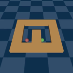
Figure 12: Pointmaze environment (Fu et al., 2020).

Appendix H Evaluating the Goodness of Network Architecture and Initialization

Can we also use PIC and POIC to evaluate the goodness of network architecture or initialization? We investigate the correlation between PIC or POIC and the normalized score of the PPO policy with different network configurations. For the comparison, we prepare 7 policy network architectures without bias term (0 layers $+$ [1, 2] layers $\times$ [4, 32, 64] hidden units; while keeping original value networks sizes, 2 layers 64 units), and 4 initializations (normal $\mathcal{N}(0,I)$, uniform $\textit{Unif}(-1,1)$, Xavier normal and Xavier uniform). Xavier Normal and Uniform are the typical initialization methods of neural networks (Glorot & Bengio, 2010). First, we measure both PIC and POIC for each policy, and then train it with PPO, during 500k steps, except for 50k steps in CartPole (see Appendix I for the detailed results).

The results are shown in Table 15, and Table 14. We can see valid positive correlations in CartPole, Pendulum, HalfCheetah, Hopper, and Walker2d with specific initialization, which are statistically significant with $p<0.05$, while we also observe the weak positive, negative, or no trends in other environments. In several domains, PIC and POIC might be used for architectural tuning without extensive RL trainings. In addition, some negative results seem consistent with empirical observations in recent RL research; the performance of many deep RL algorithms require architectural tuning for best performances (Schulman et al., 2015, 2017; Engstrom et al., 2019; Andrychowicz et al., 2021), and can be sensitive to architecture and initialization (Rajeswaran et al., 2017).

PIC	CartPole	Pendulum	MountainCar	MountainCarContinuous	Acrobot	HalfCheetah	Hopper	Walker2d
Normal (p-Value)	0.938 (0.002)	0.121 (0.796)	0.681 (0.092)	0.124 (0.791)	-0.455 (0.304)	0.891 (0.007)	0.839 (0.018)	0.782 (0.038)
Uniform (p-Value)	0.658 (0.108)	-0.172 (0.712)	-0.783 (0.037)	-0.021 (0.965)	0.502 (0.251)	0.881 (0.009)	0.649 (0.115)	0.617 (0.140)
Xavier (N) (p-Value)	0.483 (0.272)	0.438 (0.325)	-0.544 (0.207)	-0.079 (0.866)	-0.474 (0.283)	0.186 (0.689)	-0.660 (0.106)	-0.789 (0.035)
Xavier (U) (p-Value)	0.171 (0.713)	0.406 (0.366)	-0.244 (0.599)	0.667 (0.102)	-0.259 (0.574)	-0.003 (0.995)	-0.709 (0.075)	-0.965 ($>$ 0.001)

Table 14: Pearson correlation coefficient between the normalized score of different policies (network architecture and initialization) and PIC. We can see valid positive correlations in CartPole, HalfCheetah, Hopper, and Walker2d with specific initialization, which are statistically significant with $p<0.05$. The 2D-plots can be seen in Figure 13.

POIC	CartPole	Pendulum	MountainCar	MountainCarContinuous	Acrobot	HalfCheetah	Hopper	Walker2d
Normal (p-Value)	0.392 (0.385)	0.769 (0.043)	-0.229 (0.621)	0.004 (0.994)	0.177 (0.704)	0.855 (0.014)	0.476 (0.280)	0.624 (0.134)
Uniform (p-Value)	-0.087 (0.852)	0.451 (0.309))	-0.842 (0.018)	-0.059 (0.900)	-0.288 (0.532)	0.864 (0.012)	0.188 (0.686)	0.523 (0.229)
Xavier (N) (p-Value)	0.127 (0.787)	0.579 (0.173)	-0.503 (0.250)	0.373 (0.409)	-0.720 (0.068)	0.344 (0.450)	0.957 ($>$ 0.001)	-0.946 (0.001)
Xavier (U) (p-Value)	0.930 (0.002)	0.495 (0.258)	-0.406 (0.367)	-0.649 (0.114)	-0.381 (0.399)	0.080 (0.865)	0.006 (0.990)	-0.726 (0.065)

Table 15: Pearson correlation coefficient between the normalized score of different policies (network architecture and initialization) and POIC. We can see valid positive correlations in CartPole, Pendulum, HalfCheetah and Hopper with specific initialization, which are statistically significant with $p<0.05$. The 2D-plots can be seen in Figure 14.

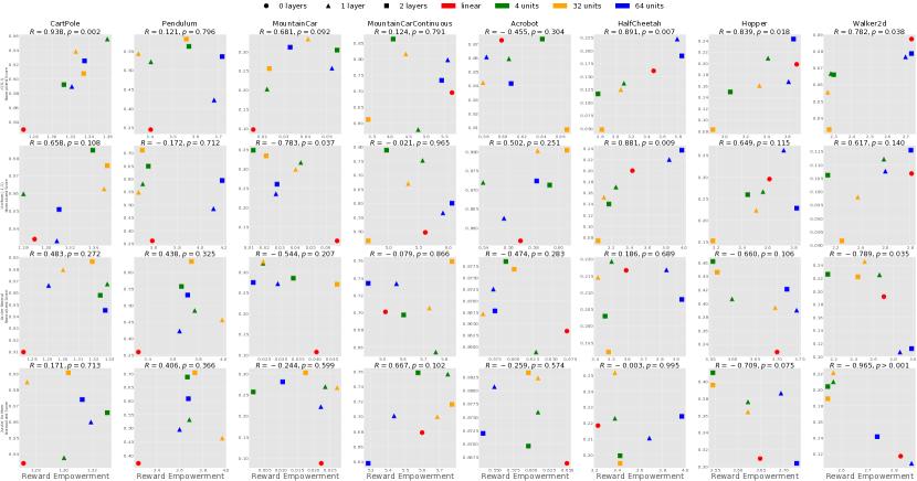
Figure 13: 2D-Scatter plots between PIC (x-axis) and the normalized score (y-axis), trained during 500k steps and averaged over 5 seeds. We test combinations of 7 network architectures (0 layers, 1 layer 4 units, 2 layers 4units) and 4 kinds of network initialization (normal, uniform, Xavier normal, Xavier uniform).

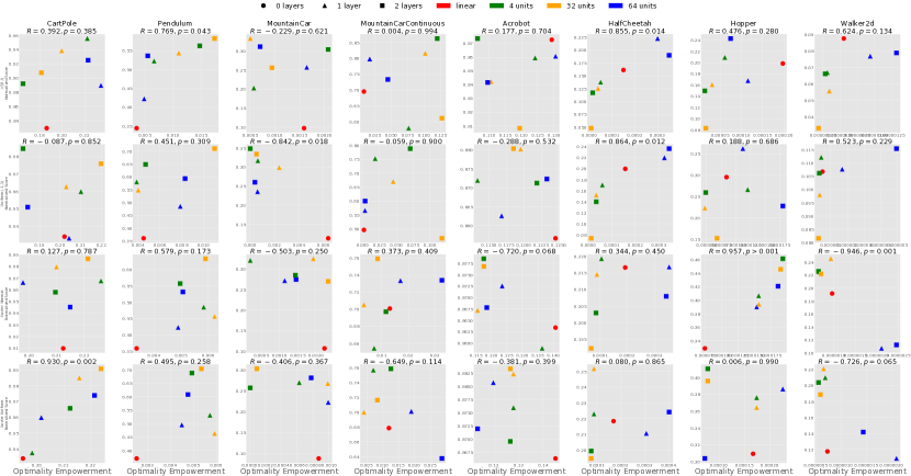
Figure 14: 2D-Scatter plots between POIC (x-axis) and the normalized score (y-axis), trained during 500k steps and averaged over 5 seeds. We test combinations of 7 network architectures (0 layers, 1 layer 4 units, 2 layers 4units) and 4 kinds of network initialization (normal, uniform, Xavier normal, Xavier uniform).

Appendix I Details of Architecture and Initialization Experiments

In this section, we presents the raw scores observed through the experiments in Appendix H. We train PPO with (64, 64) neural networks and 3 different discount factor $\gamma\in\{0.95,0.99,0.995\}$. For normalized score, we refer the algorithm-max scores in Appendix C. All results are summarized in Table 16 (average cumulative rewards), Table 17 (normalized score), Table 18 (PIC), and Table 19 (POIC).

	CartPole	Pendulum	MountainCar	MountainCarContinuous	Acrobot	HalfCheetah	Hopper	Walker2d
0L Normal	167.38	-1268.00	-189.97	37.57	-120.18	154.04	488.97	705.56
1L 4U Normal	178.85	-1134.51	-173.60	56.37	-125.43	1221.59	427.17	596.35
1L 32U Normal	191.51	-962.21	-179.17	13.59	-125.97	-221.18	367.72	743.74
1L 64U Normal	188.20	-926.62	-165.81	59.85	-133.48	-344.62	303.13	570.78
2L 4U Normal	185.68	-931.49	-168.00	43.72	-133.74	618.83	435.76	864.46
2L 32U Normal	179.36	-883.60	-168.76	69.01	-119.79	-369.87	364.67	531.89
2L 64U Normal	182.30	-852.51	-173.71	19.79	-148.21	-404.71	173.00	294.66
0L Uniform	187.37	-1243.73	-188.33	31.21	-127.21	780.81	600.25	1051.04
1L 4U Uniform	187.19	-1017.40	-175.79	18.77	-124.63	1057.68	591.57	1289.52
1L 32U Uniform	192.31	-857.24	-167.46	47.44	-120.57	652.51	632.90	946.86
1L 64U Uniform	192.84	-908.35	-169.29	31.27	-116.97	316.07	548.21	792.32
2L 4U Uniform	190.61	-829.38	-173.24	24.82	-120.39	1361.30	637.16	810.50
2L 32U Uniform	197.04	-737.45	-164.19	54.40	-120.86	364.60	598.17	922.05
2L 64U Uniform	195.37	-629.24	-165.67	-8.47	-116.90	-186.69	456.83	540.52
0L Xavier (N)	182.75	-1249.18	-189.02	37.42	-124.27	1111.14	1096.75	1170.13
1L 4U Xavier (N)	193.55	-1132.60	-172.06	43.82	-120.29	1219.57	599.91	1389.66
1L 32U Xavier (N)	193.81	-1022.30	-166.99	31.09	-126.25	1644.45	1292.61	1448.79
1L 64U Xavier (N)	196.11	-1069.38	-166.55	43.21	-122.63	1593.45	1410.29	1403.11
2L 4U Xavier (N)	189.53	-937.73	-171.75	43.82	-122.36	1048.78	634.12	1499.48
2L 32U Xavier (N)	191.96	-893.65	-170.69	36.78	-117.69	1459.96	1297.16	1645.11
2L 64U Xavier (N)	197.45	-764.92	-172.21	49.70	-118.43	1507.47	1275.05	1588.82
0L Xavier (U)	187.37	-1223.45	-190.93	37.53	-122.97	1117.23	663.19	1101.14
1L 4U Xavier (U)	192.31	-1005.49	-177.17	37.54	-116.74	1218.68	611.44	1376.33
1L 32U Xavier (U)	188.04	-945.72	-172.31	49.55	-118.81	1467.81	1202.81	1339.44
1L 64U Xavier (U)	197.10	-1055.70	-172.53	42.33	-116.03	1977.95	1268.04	1297.33
2L 4U Xavier (U)	195.00	-806.39	-171.13	25.00	-120.53	1370.19	804.70	1081.45
2L 32U Xavier (U)	193.43	-670.05	-173.58	49.16	-121.57	1758.48	1168.65	1462.36
2L 64U Xavier (U)	198.21	-640.18	-168.91	42.80	-115.60	1677.97	1080.10	1410.35

Table 16: Cumulative rewards averaged over 3 different discount factor $\gamma\in\{0.95,0.99,0.995\}$ and 5 random seeds.

	CartPole	Pendulum	MountainCar	MountainCarContinuous	Acrobot	HalfCheetah	Hopper	Walker2d
0L Normal	0.829	0.345	0.098	0.695	0.873	0.161	0.087	0.198
1L 4U Normal	0.889	0.422	0.257	0.798	0.861	0.223	0.077	0.168
1L 32U Normal	0.956	0.522	0.203	0.580	0.859	0.137	0.067	0.209
1L 64U Normal	0.938	0.544	0.333	0.816	0.842	0.125	0.056	0.161
2L 4U Normal	0.925	0.536	0.311	0.734	0.842	0.190	0.079	0.243
2L 32U Normal	0.892	0.563	0.304	0.863	0.874	0.117	0.066	0.150
2L 64U Normal	0.907	0.582	0.256	0.611	0.808	0.048	0.033	0.083
0L Uniform	0.934	0.361	0.114	0.497	0.857	0.200	0.107	0.295
1L 4U Uniform	0.933	0.485	0.236	0.566	0.863	0.220	0.108	0.362
1L 32U Uniform	0.960	0.581	0.317	0.752	0.872	0.170	0.112	0.266
1L 64U Uniform	0.963	0.549	0.299	0.670	0.880	0.152	0.098	0.223
2L 4U Uniform	0.951	0.594	0.260	0.600	0.872	0.237	0.115	0.228
2L 32U Uniform	0.985	0.649	0.348	0.788	0.871	0.140	0.106	0.259
2L 64U Uniform	0.976	0.711	0.334	0.467	0.880	0.074	0.082	0.152
0L Xavier (N)	0.910	0.359	0.107	0.701	0.863	0.217	0.192	0.329
1L 4U Xavier (N)	0.966	0.423	0.272	0.733	0.873	0.217	0.107	0.390
1L 32U Xavier (N)	0.968	0.485	0.321	0.654	0.859	0.219	0.225	0.407
1L 64U Xavier (N)	0.980	0.456	0.325	0.705	0.867	0.215	0.246	0.394
2L 4U Xavier (N)	0.945	0.532	0.275	0.734	0.868	0.208	0.112	0.421
2L 32U Xavier (N)	0.958	0.557	0.285	0.697	0.879	0.203	0.226	0.462
2L 64U Xavier (N)	0.987	0.633	0.270	0.759	0.877	0.192	0.222	0.446
0L Xavier (U)	0.934	0.371	0.088	0.679	0.866	0.218	0.118	0.309
1L 4U Xavier (U)	0.960	0.495	0.222	0.701	0.881	0.211	0.109	0.386
1L 32U Xavier (U)	0.937	0.531	0.269	0.757	0.876	0.223	0.210	0.376
1L 64U Xavier (U)	0.985	0.464	0.267	0.700	0.882	0.252	0.221	0.364
2L 4U Xavier (U)	0.974	0.608	0.281	0.638	0.872	0.224	0.142	0.304
2L 32U Xavier (U)	0.966	0.688	0.257	0.759	0.870	0.199	0.204	0.411
2L 64U Xavier (U)	0.991	0.704	0.302	0.716	0.883	0.195	0.189	0.396

Table 17: Algorithm-based normalized scores. We use the minimum values during random-sampling and the maximum values reported in Table 3 and Table 4.

	CartPole	Pendulum	MountainCar	MountainCarContinuous	Acrobot	HalfCheetah	Hopper	Walker2d
0L Normal	1.269	3.402	0.016	5.707	0.599	3.486	2.732	3.685
1L 4U Normal	1.321	3.681	0.052	5.588	0.583	3.789	2.698	3.608
1L 32U Normal	1.359	3.403	0.022	4.774	0.606	3.105	2.283	3.412
1L 64U Normal	1.326	3.348	0.041	4.433	0.579	3.065	2.267	3.330
2L 4U Normal	1.335	3.716	0.033	5.421	0.608	3.847	2.731	3.655
2L 32U Normal	1.313	3.570	0.055	4.086	0.641	2.771	2.300	3.052
2L 64U Normal	1.334	3.559	0.023	3.395	0.667	2.822	2.274	2.886
0L Uniform	1.290	3.586	0.067	5.612	0.569	3.432	2.810	3.612
1L 4U Uniform	1.309	4.112	0.027	5.907	0.556	3.838	2.599	3.722
1L 32U Uniform	1.280	3.503	0.044	5.568	0.540	3.251	2.587	3.562
1L 64U Uniform	1.349	3.466	0.040	5.327	0.583	3.119	2.376	3.509
2L 4U Uniform	1.311	4.187	0.028	6.057	0.582	3.976	2.804	3.822
2L 32U Uniform	1.339	3.552	0.013	4.968	0.593	3.172	2.134	3.443
2L 64U Uniform	1.352	3.500	0.021	4.661	0.606	3.052	2.248	3.174
0L Xavier (N)	1.275	3.326	0.040	5.516	0.670	3.592	2.705	3.699
1L 4U Xavier (N)	1.291	3.652	0.029	5.569	0.573	3.840	2.867	3.743
1L 32U Xavier (N)	1.329	3.772	0.025	5.759	0.630	3.502	2.660	3.598
1L 64U Xavier (N)	1.300	3.990	0.025	5.728	0.559	3.418	2.511	3.695
2L 4U Xavier (N)	1.327	3.716	0.022	5.432	0.575	3.934	2.984	3.721
2L 32U Xavier (N)	1.324	3.667	0.034	5.604	0.590	3.462	2.139	3.555
2L 64U Xavier (N)	1.319	3.746	0.047	5.838	0.600	3.483	2.443	3.565
0L Xavier (U)	1.271	3.240	0.022	5.599	0.649	3.229	2.825	3.648
1L 4U Xavier (U)	1.319	3.597	0.022	5.436	0.549	3.683	2.867	3.694
1L 32U Xavier (U)	1.300	3.682	0.024	5.749	0.609	3.379	2.568	3.621
1L 64U Xavier (U)	1.274	3.967	0.027	5.687	0.609	3.379	2.568	3.621
2L 4U Xavier (U)	1.313	3.673	0.010	5.285	0.533	3.970	2.736	3.728
2L 32U Xavier (U)	1.331	3.665	0.001	5.575	0.596	3.425	2.547	3.545
2L 64U Xavier (U)	1.303	3.730	0.017	5.773	0.596	3.425	2.547	3.545

Table 18: Estimated Policy Information Capacity.

	CartPole	Pendulum	MountainCar	MountainCarContinuous	Acrobot	HalfCheetah	Hopper	Walker2d
0L Normal	0.186	0.003516	0.001586	0.008363	0.129	0.000150	0.000000551	0.000198
1L 4U Normal	0.235	0.004850	0.001641	0.017159	0.131	0.000300	0.000000935	0.000116
1L 32U Normal	0.222	0.006613	0.000573	0.076397	0.124	0.000049	0.000000312	0.000061
1L 64U Normal	0.200	0.010994	0.000502	0.101649	0.111	0.000037	0.000000339	0.000031
2L 4U Normal	0.223	0.005492	0.000699	0.044784	0.109	0.000351	0.000001318	0.000075
2L 32U Normal	0.165	0.014715	0.002074	0.119891	0.106	0.000014	0.000000280	0.000014
2L 64U Normal	0.182	0.017335	0.000939	0.126900	0.119	0.000008	0.000000182	0.000016
0L Uniform	0.202	0.004520	0.006387	0.001799	0.125	0.000157	0.000000507	0.000084
1L 4U Uniform	0.204	0.007866	0.000603	0.003397	0.117	0.000323	0.000001682	0.000112
1L 32U Uniform	0.210	0.003882	0.000628	0.018515	0.113	0.000059	0.000000427	0.000120
1L 64U Uniform	0.203	0.004031	0.002376	0.045212	0.120	0.000033	0.000000341	0.000047
2L 4U Uniform	0.184	0.008297	0.000383	0.003576	0.123	0.000343	0.000004932	0.000180
2L 32U Uniform	0.182	0.004696	0.000007	0.070520	0.122	0.000034	0.000000319	0.000048
2L 64U Uniform	0.220	0.010994	0.000516	0.117416	0.119	0.000012	0.000000266	0.000067
0L Xavier (N)	0.212	0.003354	0.002235	0.013028	0.141	0.000192	0.000000957	0.000075
1L4U Xavier (N)	0.198	0.004885	0.001138	0.017027	0.123	0.000353	0.000002099	0.000153
1L32U Xavier (N)	0.226	0.005830	0.000191	0.007107	0.136	0.000104	0.000000659	0.000156
1L 64U Xavier (N)	0.210	0.006233	0.001928	0.003256	0.115	0.000088	0.000000927	0.000157
2L 4U Xavier (N)	0.215	0.005060	0.001453	0.032625	0.118	0.000342	0.000002443	0.000186
2L 32U Xavier (N)	0.210	0.004961	0.001432	0.011564	0.117	0.000084	0.000000642	0.000193
2L 64U Xavier (N)	0.221	0.005896	0.002337	0.008424	0.118	0.000067	0.000000702	0.000190
0L Xavier (U)	0.195	0.002517	0.000868	0.011988	0.145	0.000169	0.000000728	0.000167
1L 4U Xavier (U)	0.202	0.004492	0.000988	0.019024	0.120	0.000306	0.000002099	0.000226
1L 32U Xavier (U)	0.198	0.005724	0.000623	0.007098	0.128	0.000088	0.000000685	0.000174
1L 64U Xavier (U)	0.216	0.005925	0.000983	0.004143	0.128	0.000088	0.000000652	0.000174
2L 4U Xavier (U)	0.221	0.004763	0.000774	0.028628	0.113	0.000402	0.000001439	0.000072
2L 32U Xavier (U)	0.212	0.004936	0.000009	0.012626	0.127	0.000076	0.000000551	0.000078
2L 64U Xavier (U)	0.224	0.005346	0.000092	0.008398	0.127	0.000076	0.000000589	0.000078

Table 19: Estimated Policy-Optimal Information Capacity.

Appendix J Evaluating the Dynamics and Initialization Noises

In this section, we evaluate one of our information capacity metrics’ properties: can we use PIC and POIC for tuning the noise levels in MDPs that might help to learn? To answer this question, we design the experiments to observe the correlations between each metric (POIC, optimality marginal entropy, optimality conditional entropy, PIC, reward marginal entropy, reward conditional entropy, and variance) and algorithm-based normalized scores.

For the experiments, we prepare 12 cartpole environments with 3 initialization and 4 dynamics noises. In these environments, we initialize 4-dimensional states with uniform distribution $\textit{Unif}(-u_{\text{init}},u_{\text{init}})$, where $u_{\text{init}}$ is a tunable parameter $u_{\text{init}}\in\{0.05,0.1.0.15\}$, and add 1-dimensional transition noise to angular velocity with uniform distribution $\textit{Unif}(-u_{\text{dyn}},u_{\text{dyn}})$, where $u_{\text{dyn}}$ is also a tunable parameter $u_{\text{dyn}}\in\{0.0,0.03,0.05,0.1\}$. As in Section 6.2, we prepare the bag-of-architectures to measure PIC and POIC: ([0] layers $+$ [1, 2] layers $\times$ [4, 32, 64] hidden units) $\times$ [Gaussian prior $\mathcal{N}(0,I)$, Uniform prior $\textit{Unif}(-1,1)$, Xavier Normal, Xavier Uniform] $\times$ [w/ bias, w/o bias], and bag-of-algorithms (PPO, ES, DQN with different hyper-parameters) to compute the algorithm-based normalized scores (see Table 21 for each raw score).

The results are shown in Table 20. The POIC seems the best metric that positively correlates to the algorithm-based normalized scores ($R=0.860$; statistically significant with $p<0.001$), but PIC doesn’t show such a trend. This suggests that POIC might be used for tuning initialization and dynamics noises that help to learn.

Environment	Initial Noise	Dynamics Noise	$\hat{\mathcal{I}}(\mathcal{O};\Theta)$	$\hat{\mathcal{H}}(\mathcal{O})$	$\hat{\mathcal{H}}(\mathcal{O}|\Theta)$	$\hat{\mathcal{I}}(R;\Theta)$	$\hat{\mathcal{H}}(R)$	$\hat{\mathcal{H}}(R|\Theta)$	Variance	Score(A)
CartPole	0.05	0.0	0.207	0.292	0.085	1.315	3.632	2.317	17.586	0.886
	0.05	0.03	0.172	0.252	0.080	1.268	3.696	2.428	15.540	0.848
	0.05	0.05	0.151	0.222	0.071	1.233	3.723	2.490	14.024	0.856
	0.05	0.1	0.111	0.172	0.061	1.151	3.746	2.595	11.302	0.827
	0.1	0.0	0.140	0.200	0.060	1.110	3.823	2.713	12.102	0.849
	0.1	0.03	0.130	0.185	0.055	1.095	3.843	2.748	11.430	0.849
	0.1	0.05	0.120	0.172	0.052	1.076	3.853	2.776	10.826	0.847
	0.1	0.1	0.093	0.143	0.050	1.019	3.866	2.847	9.343	0.820
	0.15	0.0	0.110	0.160	0.050	0.922	3.886	2.964	9.710	0.850
	0.15	0.03	0.105	0.150	0.046	0.913	3.895	2.981	9.326	0.848
	0.15	0.05	0.098	0.142	0.044	0.901	3.899	2.999	8.951	0.828
	0.15	0.1	0.077	0.120	0.043	0.859	3.902	3.042	7.891	0.824
Correlation Coefficient: Score(A)			0.860	0.824	0.698	0.613	-0.625	-0.625	0.783	–
p-Value: Score(A)			$>$0.001	$>$0.001	0.012	0.034	0.030	0.030	0.003	–

Table 20: PIC and POIC under noisy initialization and dynamics.

		(Initialization Noise, Dynamics Noise)
Algorithm	Hyper-Parameters	(0.05, 0.0)	(0.05, 0.03)	(0.05, 0.05)	(0.05, 0.1)	(0.1, 0.0)	(0.1, 0.03)	(0.1, 0.05)	(0.1, 0.1)	(0.15, 0.0)	(0.15, 0.03)	(0.15, 0.05)	(0.15, 0.1)
PPO	(64, 64), $\gamma=0.995$	200.0	200.0	200.0	200.0	200.0	200.0	200.0	200.0	199.6	200.0	197.8	199.4
PPO	(64, 64), $\gamma=0.99$	200.0	199.7	200.0	200.0	200.0	199.2	196.5	200.0	200.0	200.0	196.2	197.2
PPO	(64, 64), $\gamma=0.95$	194.0	200.0	197.2	192.5	193.7	196.9	182.4	193.2	189.8	186.5	200.0	193.5
PPO	(128, 64), $\gamma=0.995$	200.0	200.0	200.0	197.2	200.0	200.0	200.0	200.0	199.6	199.9	200.0	199.9
PPO	(128, 64), $\gamma=0.99$	200.0	200.0	200.0	200.0	200.0	200.0	193.1	198.5	200.0	196.8	198.3	193.8
PPO	(128, 64), $\gamma=0.95$	198.1	196.1	199.3	192.2	196.1	191.0	195.3	196.1	197.4	182.5	189.3	184.9
PPO	(128, 128), $\gamma=0.995$	200.0	199.6	200.0	200.0	197.8	200.0	200.0	199.7	191.1	196.5	200.0	195.9
PPO	(128, 128), $\gamma=0.99$	200.0	200.0	200.0	200.0	200.0	200.0	197.8	200.0	198.6	200.0	199.3	199.4
PPO	(128, 128), $\gamma=0.95$	197.1	195.2	196.4	197.5	192.9	193.4	196.5	191.7	195.6	193.4	191.2	185.8
ES	(16, 16), $\sigma=0.1$	188.1	165.5	166.5	147.1	185.3	196.3	179.1	130.2	170.3	167.2	155.1	144.6
ES	(16, 16), $\sigma=0.1$, rand	197.1	161.7	175.1	175.9	186.4	170.7	185.8	140.9	167.7	173.0	159.8	167.3
ES	(64, 64), $\sigma=0.1$	168.6	159.6	187.2	170.0	160.9	150.2	171.9	115.7	173.3	150.0	170.4	141.5
ES	(64, 64), $\sigma=0.1$, rand	168.0	177.0	170.8	112.7	161.4	174.3	169.4	131.1	173.4	166.6	138.9	128.2
DQN	(100, 100), $\gamma=0.95$	133.2	127.1	131.4	131.5	123.4	102.5	87.3	128.8	116.0	134.8	130.7	117.8
DQN	(100, 100), $\gamma=0.99$	185.2	169.6	114.7	145.0	163.1	174.3	177.2	193.1	169.0	157.8	163.6	171.4
DQN	(200, 200), $\gamma=0.95$	132.2	97.2	73.9	118.6	96.2	135.6	113.0	128.8	106.0	107.3	117.0	122.6
DQN	(200, 200), $\gamma=0.99$	195.5	196.0	179.7	194.9	195.9	149.4	172.2	182.4	184.8	183.2	167.3	189.4
DQN	(50, 50), $\gamma=0.95$	161.3	123.5	166.4	91.5	98.6	101.3	156.2	113.3	132.4	127.5	121.0	90.2
DQN	(50, 50), $\gamma=0.99$	176.3	153.7	169.4	172.8	170.0	179.8	163.6	137.0	168.8	155.2	150.8	167.9
DQN	(50, 50, 50), $\gamma=0.95$	87.7	102.7	103.0	101.6	84.4	114.5	64.8	134.2	108.1	119.4	93.1	111.0
DQN	(50, 50, 50), $\gamma=0.99$	159.8	164.1	192.6	164.7	185.6	163.3	180.2	160.5	153.9	188.6	165.2	185.3
$r_{\text{ave}}^{\text{algo}}$	–	178.2	170.9	172.6	166.9	171.0	171.1	170.6	165.5	171.2	170.8	166.9	166.0
$r_{\max}^{\text{algo}}$	–	200.0	200.0	200.0	200.0	200.0	200.0	200.0	200.0	200.0	200.0	200.0	199.9
$r_{\min}^{\text{rand}}$	–	8.742	8.752	8.759	8.789	8.137	8.139	8.161	8.184	7.479	7.482	7.482	7.476

Table 21: Performance of a variety of algorithms in CartPole with initialization and dynamics noises. The results are averaged over 5 random seeds. We change 2 hyper-parameters, architecture of neural networks and discount factor $\gamma$.

Appendix K Our Information Capacity Metrics based on Channel Capacity

In previous works (Klyubin et al., 2005; Tishby & Polani, 2011), empowerment is originally defined with channel capacity between future state and n-step action sequence, instead of mutual information.

Following these definition, we extensively evaluate the variants of our PIC and POIC, based on channel capacity:

$$\begin{split}&\text{Policy Information Capacity: }~{}\underset{p(\theta)}{\max}~{}\mathcal{I}(R;\Theta),\\ &\text{Policy-Optimal Information Capacity: }~{}\underset{p(\theta)}{\max}~{}\mathcal{I}(\mathcal{O};\Theta).\end{split}$$ (5)

The experimental settings are similar to Section 6.2; we investigate the correlation between channel-capacity-based information capacity metrics, and algorithm- or random-sampling-based normalized score. To take the maximum over parameter distribution in Equation 5, we prepare a “bag-of-policy-architectures” in practice: ([0] layers $+$ [1, 2] layers $\times$ [4, 32, 64] hidden units) $\times$ [Gaussian prior $\mathcal{N}(0,I)$, Uniform prior $\textit{Unif}(-1,1)$, Xavier Normal, Xavier Uniform] $\times$ [w/ bias, w/o bias], which amounts to 56 different parameter distributions $p(\theta)$.

The results are shown in Figure 16 (also shown in Figure 15 and Table 22). POIC seems to positively correlate to the algorithm-based normalized score ($R=0.707$; statistically significant with $p<0.01$), which can be regarded as the more realistic of the two task difficulty scores. On the other hand, PIC also shows a weak positive correlation with the random-sampling-based normalized score ($R=0.421$). These results show the similar trends with our definition of PIC and POIC, based on mutual information.

Figure 15: [Channel Capacity version]: 2D-Scatter plots between each metric (State dimension, action dimension, episode horizon, and normalized scores; x-axis) and each normalized score (algorithm-based (top) and random-sampling-based (bottom); y-axis).

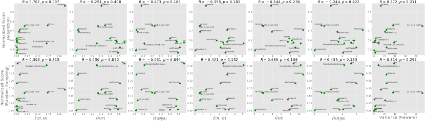
Figure 16: [Channel Capacity version]: 2D-Scatter plots between each metric (x-axis) and normalized scores (algorithm-based (top) and random-sampling-based (bottom) ; y-axis); see Table 22 for the details. Variance (last column) approximately corresponds to the metric proposed by Oller et al. (2020). POIC positively correlates with algorithm-based normalized score ($R=0.707$; statistically significant with $p<0.01$), the more realistic of the two task difficulty scores.

Environment	Score(A)	Score(R)	$\hat{\mathcal{I}}(\mathcal{O};\Theta)$	$\hat{\mathcal{H}}(\mathcal{O})$	$\hat{\mathcal{H}}(\mathcal{O}|\Theta)$	$\hat{\mathcal{I}}(R;\Theta)$	$\hat{\mathcal{H}}(R)$	$\hat{\mathcal{H}}(R|\Theta)$	Variance	State dim	Action dim	Horizon
CartPole	0.970	0.141	0.225996	0.303	0.077	1.363	3.687	2.324	12.610	4	2	200
Pendulum	0.710	0.242	0.013944	0.034	0.020	4.036	10.901	6.865	23.223	3	1	200
MountainCar	0.491	0.001	0.002337	0.016	0.014	0.047	0.070	0.023	0.054	2	3	200
MountainCarContinuous	0.566	0.305	0.140193	0.250	0.110	6.100	10.331	4.230	8.022	2	1	999
Acrobot	0.759	0.121	0.145020	0.344	0.199	0.670	1.672	1.002	35.891	6	3	500
Ant	0.575	0.316	0.003742	0.567	0.563	3.529	8.730	5.201	37.830	111	8	1000
HalfCheetah	0.523	0.183	0.000402	0.515	0.515	3.195	9.148	5.953	23.468	17	6	1000
Hopper	0.619	0.007	0.000226	0.403	0.403	4.214	7.780	3.565	3.006	11	3	1000
Walker2d	0.583	0.075	5.1e-05	0.480	0.480	4.027	7.445	3.418	0.403	17	6	1000
Humanoid	0.466	0.008	2.9e-05	0.494	0.494	3.810	7.870	4.061	1.917	376	17	1000
cheetah run	0.597	0.030	0.000483	0.473	0.472	2.708	8.335	5.627	1.972	17	6	1000
reacher easy	0.691	0.069	0.010335	0.044	0.034	0.622	3.866	3.244	20.669	6	2	1000
ball_in_cup catch	0.752	0.118	0.036467	0.264	0.227	0.553	1.942	1.389	91.454	8	2	1000
Correlation Coefficient: Score(A)	–	0.139	0.707	-0.251	-0.473	-0.395	-0.344	-0.244	0.372	-0.427	-0.544	-0.452
p-Value: Score(A)	–	0.651	0.007	0.408	0.103	0.182	0.250	0.422	0.211	0.146	0.055	0.121
Correlation Coefficient: Score(R)	0.139	–	0.303	0.050	-0.061	0.421	0.469	0.439	0.314	-0.183	-0.259	-0.016
p-Value: Score(R)	0.651	–	0.315	0.870	0.844	0.152	0.106	0.133	0.297	0.549	0.393	0.959

Table 22: [Channel Capacity version]: POIC $\hat{\mathcal{I}}(\mathcal{O};\Theta)$, optimality marginal entropy $\hat{\mathcal{H}}(\mathcal{O})$, optimality conditional entropy $\hat{\mathcal{H}}(\mathcal{O}|\Theta)$, PIC $\hat{\mathcal{I}}(R;\Theta)$, reward marginal entropy $\hat{\mathcal{H}}(R)$, reward conditional entropy $\hat{\mathcal{H}}(R|\Theta)$, normalized variance of return in standard RL benchmark environments, Pearson correlation coefficient to the algorithm-based normalized score (Score(A)), and the random-sampling-based normalized score (Score(R)). We prepare the bags of policy architectures, 56 variants in total; ([0] layers $+$ [1, 2] layers $\times$ [4, 32, 64] units) $\times$ [Gaussian prior $\mathcal{N}(0,I)$, Uniform prior $\textit{Unif}(-1,1)$, Xavier Normal, Xavier Uniform] $\times$ [w/ bias, w/o bias]. Since we consider the definition based on channel capacity here, we take the maximum value of each information capacity metrics over these policy architectures. The results suggest that POIC seems to positively correlate with algorithm-based normalized score ($R=0.707$; statistically significant with $p<0.01$) better than all other alternatives including variance of returns (Oller et al., 2020).

References

- Abdolmaleki et al. (2018) Abdolmaleki, A., Springenberg, J. T., Tassa, Y., Munos, R., Heess, N., and Riedmiller, M. Maximum a posteriori policy optimisation. In International Conference on Learning Representations, 2018.
- Andrychowicz et al. (2021) Andrychowicz, M., Raichuk, A., Stańczyk, P., Orsini, M., Girgin, S., Marinier, R., Hussenot, L., Geist, M., Pietquin, O., Michalski, M., Gelly, S., and Bachem, O. What matters for on-policy deep actor-critic methods? a large-scale study. In International Conference on Learning Representations, 2021.
- Azar et al. (2017) Azar, M. G., Osband, I., and Munos, R. Minimax regret bounds for reinforcement learning. In International Conference on Machine Learning, 2017.
- Barber & Agakov (2004) Barber, D. and Agakov, F. The im algorithm : A variational approach to information maximization. In Advances in neural information processing systems, 2004.
- Belghazi et al. (2018) Belghazi, M. I., Baratin, A., Rajeshwar, S., Ozair, S., Bengio, Y., Courville, A., and Hjelm, D. Mutual information neural estimation. In International Conference on Machine Learning, 2018.
- Bellemare et al. (2013) Bellemare, M. G., Naddaf, Y., Veness, J., and Bowling, M. The arcade learning environment: An evaluation platform for general agents. Journal of Artificial Intelligence Research, 2013.
- Bellemare et al. (2017) Bellemare, M. G., Dabney, W., and Munos, R. A distributional perspective on reinforcement learning. In International Conference on Machine Learning, 2017.
- Boucheron et al. (2013) Boucheron, S., Lugosi, G., and Massart, P. Concentration Inequalities: A Nonasymptotic Theory of Independence. Oxford University Press, Oxford, UK, 2013.
- Brockman et al. (2016) Brockman, G., Cheung, V., Pettersson, L., Schneider, J., Schulman, J., Tang, J., and Zaremba, W. Openai gym. arXiv preprint arXiv:1606.01540, 2016.
- Campos et al. (2020) Campos, V. A., Trott, A., Xiong, C., Socher, R., i Nieto, X. G., and Torres, J. Explore, discover and learn: Unsupervised discovery of state-covering skills. In International Conference on Machine Learning, 2020.
- Chua et al. (2018) Chua, K., Calandra, R., McAllister, R., and Levine, S. Deep reinforcement learning in a handful of trials using probabilistic dynamics models. In Advances in Neural Information Processing Systems, 2018.
- Dann & Brunskill (2015) Dann, C. and Brunskill, E. Sample complexity of episodic fixed-horizon reinforcement learning. In Advances in Neural Information Processing Systems, 2015.
- Dann et al. (2018) Dann, C., Jiang, N., Krishnamurthy, A., Agarwal, A., Langford, J., and Schapire, R. E. On oracle-efficient pac rl with rich observations. In Advances in Neural Information Processing Systems, 2018.
- Dietterich (1998) Dietterich, T. G. The maxq method for hierarchical reinforcement learning. In International Conference on Machine Learning, 1998.
- Du et al. (2019) Du, S. S., Zhai, X., Poczos, B., and Singh, A. Gradient descent provably optimizes over-parameterized neural networks. In International Conference on Learning Representations, 2019.
- Engstrom et al. (2019) Engstrom, L., Ilyas, A., Santurkar, S., Tsipras, D., Janoos, F., Rudolph, L., and Madry, A. Implementation matters in deep rl: A case study on ppo and trpo. In International Conference on Learning Representations, 2019.
- Eysenbach et al. (2019) Eysenbach, B., Gupta, A., Ibarz, J., and Levine, S. Diversity is all you need: Learning diverse skills without a reward function. In international conference on learning representations, 2019.
- Florensa et al. (2017) Florensa, C., Duan, Y., and Abbeel, P. Stochastic neural networks for hierarchical reinforcement learning. In International conference on learning representations, 2017.
- Fox et al. (2016) Fox, R., Pakman, A., and Tishby, N. Taming the noise in reinforcement learning via soft updates. In Conference on Uncertainty in Artificial Intelligence, 2016.
- Fu et al. (2020) Fu, J., Kumar, A., Nachum, O., Tucker, G., and Levine, S. D4rl: Datasets for deep data-driven reinforcement learning. arXiv preprint arXiv:2004.07219, 2020.
- Fujimoto et al. (2018) Fujimoto, S., van Hoof, H., and Meger, D. Addressing function approximation error in actor-critic methods. In International Conference on Machine Learning, 2018.
- Glorot & Bengio (2010) Glorot, X. and Bengio, Y. Understanding the difficulty of training deep feedforward neural networks. In International Conference on Artificial Intelligence and Statistics, 2010.
- Gregor et al. (2016) Gregor, K., Rezende, D. J., and Wierstra, D. Variational intrinsic control. arXiv preprint arXiv:1611.07507, 2016.
- Gu et al. (2016a) Gu, S., Lillicrap, T., Ghahramani, Z., Turner, R. E., and Levine, S. Q-prop: Sample-efficient policy gradient with an off-policy critic. arXiv preprint arXiv:1611.02247, 2016a.
- Gu et al. (2016b) Gu, S., Lillicrap, T., Sutskever, I., and Levine, S. Continuous deep q-learning with model-based acceleration. In International Conference on Machine Learning, 2016b.
- Gu et al. (2017) Gu, S. S., Lillicrap, T., Turner, R. E., Ghahramani, Z., Schölkopf, B., and Levine, S. Interpolated policy gradient: Merging on-policy and off-policy gradient estimation for deep reinforcement learning. In Advances in neural information processing systems, 2017.
- Haarnoja et al. (2017) Haarnoja, T., Tang, H., Abbeel, P., and Levine, S. Reinforcement learning with deep energy-based policies. In International Conference on Machine Learning, 2017.
- Haarnoja et al. (2018) Haarnoja, T., Zhou, A., Hartikainen, K., Tucker, G., Ha, S., Tan, J., Kumar, V., Zhu, H., Gupta, A., Abbeel, P., and Levine, S. Soft actor-critic algorithms and applications. arXiv preprint arXiv:1812.05905, 2018.
- Hafner et al. (2020a) Hafner, D., Lillicrap, T., Ba, J., and Norouzi, M. Dream to control: Learning behaviors by latent imagination. In International Conference on Learning Representations, 2020a.
- Hafner et al. (2020b) Hafner, D., Ortega, P. A., Ba, J., Parr, T., Friston, K., and Heess, N. Action and perception as divergence minimization. arXiv preprint arXiv:2009.01791, 2020b.
- Hansen et al. (2020) Hansen, S., Dabney, W., Barreto, A., Warde-Farley, D., de Wiele, T. V., and Mnih, V. Fast task inference with variational intrinsic successor features. In International Conference on Learning Representations, 2020.
- Hessel et al. (2018) Hessel, M., Modayil, J., Van Hasselt, H., Schaul, T., Ostrovski, G., Dabney, W., Horgan, D., Piot, B., Azar, M., and Silver, D. Rainbow: Combining improvements in deep reinforcement learning. In AAAI Conference on Artificial Intelligence, 2018.
- Jaksch et al. (2010) Jaksch, T., Ortner, R., and Auer, P. Near-optimal regret bounds for reinforcement learning. Journal of Machine Learning Research, 2010.
- Janner et al. (2019) Janner, M., Fu, J., Zhang, M., and Levine, S. When to trust your model: Model-based policy optimization. In Advances in Neural Information Processing Systems, 2019.
- Jaques et al. (2017) Jaques, N., Gu, S., Bahdanau, D., Hernández-Lobato, J. M., Turner, R. E., and Eck, D. Sequence tutor: Conservative fine-tuning of sequence generation models with kl-control. In International Conference on Machine Learning, 2017.
- Jiang et al. (2017) Jiang, N., Krishnamurthy, A., Agarwal, A., Langford, J., and Schapire, R. E. Contextual decision processes with low Bellman rank are PAC-learnable. In International Conference on Machine Learning, 2017.
- Jin et al. (2018) Jin, C., Allen-Zhu, Z., Bubeck, S., and Jordan, M. I. Is q-learning provably efficient? In Advances in Neural Information Processing Systems, 2018.
- Jin et al. (2020) Jin, C., Yang, Z., Wang, Z., and Jordan, M. I. Provably efficient reinforcement learning with linear function approximation. In Conference on Learning Theory, 2020.
- Jung et al. (2011) Jung, T., Polani, D., and Stone, P. Empowerment for continuous agent—environment systems. Adaptive Behavior, 2011.
- Kalashnikov et al. (2018) Kalashnikov, D., Irpan, A., Pastor, P., Ibarz, J., Herzog, A., Jang, E., Quillen, D., Holly, E., Kalakrishnan, M., Vanhoucke, V., and Levine, S. QT-Opt: Scalable deep reinforcement learning for vision-based robotic manipulation. In Conference on Robot Learning, 2018.
- Kearns & Singh (2002) Kearns, M. and Singh, S. Near-optimal reinforcement learning in polynomial time. Machine Learning, 2002.
- Klyubin et al. (2005) Klyubin, A. S., Polani, D., and Nehaniv, C. L. All else being equal be empowered. In Advances in Artificial Life, 2005.
- Konidaris & Barto (2009) Konidaris, G. and Barto, A. Skill discovery in continuous reinforcement learning domains using skill chaining. In Advances in Neural Information Processing Systems, 2009.
- Laskin et al. (2020) Laskin, M., Lee, K., Stooke, A., Pinto, L., Abbeel, P., and Srinivas, A. Reinforcement learming with augmented data. In Advances in Neural Information Processing Systems, 2020.
- Leibfried et al. (2019) Leibfried, F., Pascual-Díaz, S., and Grau-Moya, J. A unified bellman optimality principle combining reward maximization and empowerment. In Advances in Neural Information Processing Systems, 2019.
- Levine (2018) Levine, S. Reinforcement Learning and Control as Probabilistic Inference: Tutorial and review. arXiv preprint arXiv:1805.00909, 2018.
- Li et al. (2017) Li, H., Xu, Z., Taylor, G., Studer, C., and Goldstein, T. Visualizing the loss landscape of neural nets. arXiv preprint arXiv:1712.09913, 2017.
- Lillicrap et al. (2016) Lillicrap, T. P., Hunt, J. J., Pritzel, A., Heess, N., Erez, T., Tassa, Y., Silver, D., and Wierstra, D. Continuous control with deep reinforcement learning. In International Conference on Learning Representations, 2016.
- Maillard et al. (2014) Maillard, O.-A., Mann, T. A., and Mannor, S. How hard is my mdp?” the distribution-norm to the rescue”. In Advances in Neural Information Processing Systems, 2014.
- McGovern & Barto (2001) McGovern, A. and Barto, A. G. Automatic discovery of subgoals in reinforcement learning using diverse density. In International Conference on Machine Learning, 2001.
- Mnih et al. (2015) Mnih, V., Kavukcuoglu, K., Silver, D., Rusu, A. A., Veness, J., Bellemare, M. G., Graves, A., Riedmiller, M., Fidjeland, A. K., Ostrovski, G., et al. Human-level control through deep reinforcement learning. Nature, 2015.
- Mohamed & Rezende (2015) Mohamed, S. and Rezende, D. J. Variational information maximisation for intrinsically motivated reinforcement learning. In Advances in Neural Information Processing Systems, 2015.
- Nachum et al. (2019) Nachum, O., Gu, S., Lee, H., and Levine, S. Near-optimal representation learning for hierarchical reinforcement learning. In international conference on learning representations, 2019.
- Oller et al. (2020) Oller, D., Glasmachers, T., and Cuccu, G. Analyzing reinforcement learning benchmarks with random weight guessing. In International Conference on Autonomous Agents and Multi-Agent Systems, 2020.
- Peng et al. (2019) Peng, X. B., Kumar, A., Zhang, G., and Levine, S. Advantage-Weighted Regression: Simple and scalable off-policy reinforcement learning. arXiv preprint arXiv:1910.00177, 2019.
- Pong et al. (2018) Pong, V., Gu, S., Dalal, M., and Levine, S. Temporal difference models: Model-free deep rl for model-based control. arXiv preprint arXiv:1802.09081, 2018.
- Pong et al. (2020) Pong, V. H., Dalal, M., Lin, S., Nair, A., Bahl, S., and Levine, S. Skew-fit: State-covering self-supervised reinforcement learning. In International Conference on Machine Learning, 2020.
- Poole et al. (2019) Poole, B., Ozair, S., Van Den Oord, A., Alemi, A., and Tucker, G. On variational bounds of mutual information. In International Conference on Machine Learning, 2019.
- Rajeswaran et al. (2017) Rajeswaran, A., Lowrey, K., Todorov, E. V., and Kakade, S. M. Towards generalization and simplicity in continuous control. In Advances in Neural Information Processing Systems, 2017.
- Rawlik et al. (2012) Rawlik, K., Toussaint, M., and Vijayakumar, S. On stochastic optimal control and reinforcement learning by approximate inference. In International Joint Conference on Artificial Intelligence, 2012.
- Recht (2018) Recht, B. A tour of reinforcement learning: The view from continuous control. arXiv preprint arXiv:1806.09460, 2018.
- Salimans et al. (2017) Salimans, T., Ho, J., Chen, X., Sidor, S., and Sutskever, I. Evolution strategies as a scalable alternative to reinforcement learning. arXiv preprint arXiv:1703.03864, 2017.
- Saxe et al. (2019) Saxe, A. M., Bansal, Y., Dapello, J., Advani, M., Kolchinsky, A., Tracey, B. D., and Cox, D. D. On the information bottleneck theory of deep learning. Journal of Statistical Mechanics: Theory and Experiment, 2019.
- Schulman et al. (2015) Schulman, J., Levine, S., Moritz, P., Jordan, M., and Abbeel, P. Trust region policy optimization. In International Conference on Machine Learning, 2015.
- Schulman et al. (2017) Schulman, J., Wolski, F., Dhariwal, P., Radford, A., and Klimov, O. Proximal policy optimization algorithms. arXiv preprint arXiv:1707.06347, 2017.
- Sharma et al. (2020a) Sharma, A., Ahn, M., Levine, S., Kumar, V., Hausman, K., and Gu, S. Emergent real-world robotic skills via unsupervised off-policy reinforcement learning. In Robotics: Science and Systems, 2020a.
- Sharma et al. (2020b) Sharma, A., Gu, S., Levine, S., Kumar, V., and Hausman, K. Dynamics-aware unsupervised discovery of skills. In International conference on learning representations, 2020b.
- Smith & Le (2017) Smith, S. L. and Le, Q. V. A bayesian perspective on generalization and stochastic gradient descent. arXiv preprint arXiv:1710.06451, 2017.
- Smith et al. (2017) Smith, S. L., Kindermans, P.-J., Ying, C., and Le, Q. V. Don’t decay the learning rate, increase the batch size. arXiv preprint arXiv:1711.00489, 2017.
- Strehl et al. (2006) Strehl, A. L., Li, L., Wiewiora, E., Langford, J., and Littman, M. L. Pac model-free reinforcement learning. In International Conference on Machine Learning, 2006.
- Strehl et al. (2009) Strehl, A. L., Li, L., and Littman, M. L. Reinforcement learning in finite mdps: Pac analysis. Journal of Machine Learning Research, 2009.
- Tassa et al. (2018) Tassa, Y., Doron, Y., Muldal, A., Erez, T., Li, Y., de Las Casas, D., Budden, D., Abdolmaleki, A., Merel, J., Lefrancq, A., Lillicrap, T., and Riedmiller, M. Deepmind control suite. arXiv preprint arXiv:1801.00690, 2018.
- Tishby & Polani (2011) Tishby, N. and Polani, D. Information theory of decisions and actions. In Perception-action cycle. Springer, 2011.
- Todorov et al. (2012) Todorov, E., Erez, T., and Tassa, Y. Mujoco: A physics engine for model-based control. In International Conference on Intelligent Robots and Systems, 2012.
- Todorov et al. (2006) Todorov, E. et al. Linearly-solvable markov decision problems. In Advances in Neural Information Processing Systems, 2006.
- Toussaint & Storkey (2006) Toussaint, M. and Storkey, A. Probabilistic inference for solving discrete and continuous state markov decision processes. In Proceedings of the 23rd international conference on Machine learning, pp. 945–952, 2006.
- Wang et al. (2020) Wang, R., Salakhutdinov, R. R., and Yang, L. Reinforcement learning with general value function approximation: Provably efficient approach via bounded eluder dimension. In Advances in Neural Information Processing Systems, 2020.
- Warde-Farley et al. (2019) Warde-Farley, D., de Wiele, T. V., Kulkarni, T. D., Ionescu, C., Hansen, S., and Mnih, V. Unsupervised control through non-parametric discriminative rewards. In international conference on learning representations, 2019.
- Yang et al. (2020) Yang, Z., Jin, C., Wang, Z., Wang, M., and Jordan, M. Provably efficient reinforcement learning with kernel and neural function approximations. In Advances in Neural Information Processing Systems, 2020.