Characterizing and Improving the Robustness
of Self-Supervised Learning through
Background Augmentations

Abstract

Recent progress in self-supervised learning has demonstrated promising results in multiple visual tasks. An important ingredient in high-performing self-supervised methods is the use of data augmentation by training models to place different augmented views of the same image nearby in embedding space. However, commonly used augmentation pipelines treat images holistically, ignoring the semantic relevance of parts of an image—e.g. a subject vs. a background—which can lead to the learning of spurious correlations. Our work addresses this problem by investigating a class of simple, yet highly effective “background augmentations”, which encourage models to focus on semantically-relevant content by discouraging them from focusing on image backgrounds. Through a systematic investigation, we show that background augmentations lead to substantial improvements in performance across a spectrum of state-of-the-art self-supervised methods (MoCo-v2, BYOL, SwAV) on a variety of tasks, e.g. $\sim+$1-2% gains on ImageNet, enabling performance on par with the supervised baseline. Further, we find the improvement in limited-labels settings is even larger (up to 4.2%). Background augmentations also improve robustness to a number of distribution shifts, including natural adversarial examples, ImageNet-9, adversarial attacks, ImageNet-Renditions. We also make progress in completely unsupervised saliency detection, in the process of generating saliency masks used for background augmentations.

Keywords: self-supervised learning, contrastive learning, representation learning, background augmentation, out-of-distribution generalization, robustness

1 Introduction

Learning useful representations in the absence of labels is a critical challenge in machine learning. Recently, self-supervised (SSL) methods such as SimCLR (Chen et al., 2020a), MoCo-v2 (He et al., 2020; Chen et al., 2020c), BYOL (Grill et al., 2020), and SwAV (Caron et al., 2020) have risen to prominence because they are able to produce high-quality representations that rival supervised representations on vision tasks. These methods differ in the details of their approach—e.g. some are instance based (MoCo-v2, SimCLR) while others are cluster based (SwAV), some explicitly utilize negatives while others do not (BYOL), and some use a memory bank (MoCo-v2). In fact, competitive performance has recently been achieved by SimSiam (Chen and He, 2020) without any of these additions. However, a central ingredient common to all high performing SSL methods is their reliance on data augmentation as a means of encoding desired invariances. Two views of an image are created via independent samples from the data augmentation pipeline, and the objective is view-invariance, i.e. the encoder is trained to place them near each other in representational space. Thus, the choice of data augmentation is critical, as augmentations and the invariances they encourage are the primary teaching signal these methods utilize to create semantically meaningful representations.

In fact, Chen et al. (2020a) explored a large space of standard augmentations and demonstrated that the choice of these augmentations can have dramatic effects on performance. However, this standard suite of augmentations used in most SSL methods was modified from augmentations designed for supervised approaches. It may therefore be useful to design new augmentation schemes for SSL that specifically target semantic focus for this setting.

A parallel line of inquiry has found that supervised models often rely on non-semantic features that may nonetheless be predictive at test time. Models often overly focus on backgrounds (Xiao et al., 2021a; Sehwag et al., 2020; Beery et al., 2018), are brittle to distribution shift in foreground-background statistics, and rely on high-frequency information (Jo and Bengio, 2017; Ilyas et al., 2019). Models are also susceptible to adversarial attacks (Goodfellow et al., 2015; Jo and Bengio, 2017), often rely on texture over shape (Geirhos et al., 2019, 2020; Hermann et al., 2020) and are brittle to distribution shift in local texture (e.g. paintings, sculpture, Hendrycks et al. (2021)) as well as to corruptions (e.g. blur, contrast, Hendrycks and Dietterich (2019)). Importantly, the benefits or limitations of a modeling choice on robustness are not apparent from metrics on standard tasks (Hendrycks et al., 2019a). All of these results showcase the need for comprehensive model evaluation across diverse data sets and settings. We broadly encompass such comprehensive evaluation under robustness, e.g. robustness to distribution shifts (e.g. paintings, blurring, different background statistics), robustness to adversarial attacks, robustness to label scarcity.

While there has been much work investigating robustness properties in the supervised setting, the self-supervised setting has received relatively less attention. As SSL methods shrink the gap to their supervised counterparts, it has become increasingly important to characterize their robustness properties and gain a more holistic understanding. The aim of this work is twofold: characterizing the robustness of high performing SSL methods and investigating approaches for improved semantic focus via a class of augmentations called background augmentations.

We conduct a systematic, comprehensive investigation of the robustness properties of SSL methods as well as the impact of background augmentations in improving semantic focus across a) a spectrum of high performing SSL methods, b) training durations, c) three variants of background augmentations, d) different foreground extraction methods used in background augmentations, and e) a wide range of downstream data sets and tasks, including 17 distribution shift settings.

Specifically, we study three classes of approaches: BG_RM, in which a subset of backgrounds are removed during the augmentation process, BG_Random, in which backgrounds are replaced with random backgrounds from other images in the mini-batch, and BG_Swaps, in which a selection of backgrounds are swapped between positive and negative images to match backgrounds across the query and the negative, thereby explicitly penalizing background focus.

We highlight the following contributions:

• Novel background augmentation method. We develop and analyze a novel, highly effective background augmentation method BG_Swaps, which manipulates the backgrounds of positives and negatives in a structured manner, yielding large performance and robustness benefits.

• Sizeable performance benefits. We show sizeable performance improvements for all view-invariant SSL methods, yielding consistent improvements of $\sim$1-2% in linear evaluation on ImageNet; these improvements allow us to reach an accuracy of 76.1% (63.8%) on ImageNet (ImageNet-v2), on par with the standard supervised baseline 76.4% (63.8%) for ResNet-50. Further, background augmentations enable us to reach a benchmark accuracy of 74.4%, outperforming Barlow Twins (Zbontar et al., 2021), MoCo-v3 (Chen et al., 2021) and BYOL trained for 800-1000 epochs in only 100 epochs; this result takes a large step forward in reducing the amount of training required for competitive performance in SSL.

  In the limited-label setting, we show the performance benefits are even larger, e.g. in the 1% (ImageNet) label setting, BG_Swaps confers a 4.0% accuracy gain for MoCo-v2 and in the 10% label setting BG_Random enables BYOL to reach 72% accuracy using only 10% of ImageNet labels.

• Improved robustness. We find that background augmentations (especially BG_Swaps) lead to significantly improved robustness in many settings including ImageNet-9 (shift in foreground-background statistics), ImageNet-A (natural adversarial examples), ImageNet-R (ImageNet-Renditions), against adversarial attack, and ImageNet ReaL.

• Scientific Insight. We investigate the impact of background augmentations in a) the supervised setting and b) RotNet, and find that they do not confer a performance gain, giving us insight into when and how background augmentations work. We also gain further insight by shape-bias probing as well as by systematically perturbing the quality of the augmentations.

• Improvement in saliency detection. In order to separate foregrounds and backgrounds without any supervision, we also make progress in completely unsupervised saliency detection, matching or outperforming weakly supervised as well as many supervised methods.

2 Methods

2.1 Self-Supervised Learning Methods

We consider a diverse test bed of high performing self-supervised learning methods: MoCo-v2 (Chen et al., 2020c), BYOL (Grill et al., 2020), and SwAV (Caron et al., 2020) to ensure generality of our results. As in the respective original works, we use a standard ResNet-50 (He et al., 2016) as the default architecture in all experiments (SSL and supervised) unless otherwise noted. A small subset of our experiments are based on RotNet(Gidaris et al., 2018), using an AlexNet (Krizhevsky et al., 2012) architecture following the respective original work. All reported numbers are based on our reproduction unless otherwise stated. Where possible, we follow the protocol from the original works.

Here, we provide a brief overview of MoCo-v2, BYOL and SwAV and some implementation details, with further details in Appendix A. We defer an overview of RotNet to Section 4.10 and relegate implementation details to Appendix A.

Overview.

Broadly, each method uses a pair of Siamese networks (Bromley et al., 1994)—i.e. weight-sharing neural networks, to encode differently augmented “views” of the same image and maximize similarity between them, thereby encouraging the learning of “desirable” invariances. Concretely, two views $v_{s},v_{t}$ of an image $x$ are generated by sampling from a random augmentation pipeline. The student network $f_{\theta}$ is used to encode $v_{s}$ as $z_{s}=f_{\theta}(v_{s})$ and similarly the teacher network $f_{\xi}$, is used to encode $v_{t}$ as $z_{t}=f_{\xi}(v_{t})$. Then, $z_{s}$ is used to predict a target generated from $z_{t}$; the specific form of this pretext prediction task varies with the SSL method. Learning/“pre-training” is by optimization of the prediction loss over $\theta$.

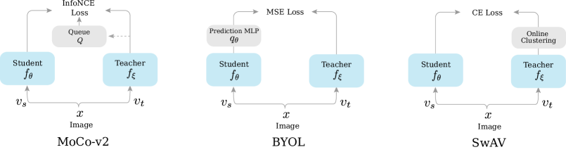
Figure 1: Schematic of Siamese SSL methods. A simplified schematic of the Siamese SSL methods in our test bed. Dashed line in MoCo-v2 denotes enqueuing the positives $k^{+}$ from the previous mini-batch (and dequeuing the oldest mini-batch).

MoCo-v2 is an instance of contrastive learning (Hadsell et al., 2006), a framework for learning representations from data that are organized into similar/dissimilar pairs. The prediction task in MoCo-v2 is one of instance discrimination: a differently augmented view of the same image $x$ needs to be discriminated from a set $Q$ of “distractors”—views of images different from $x$, in a ($|Q|+1$)-way classification. Two images form a similar/positive pair if they are views of the same image and otherwise form a negative pair. MoCo-v2 uses the InfoNCE (Oord et al., 2018) loss for this task and instantiates $Q$ as a queue comprised of previous mini-batches of $\ell_{2}$ normalized outputs from the teacher. The prediction is $\bar{z}_{s}$ and the target is $\bar{z}_{t}$, where $\bar{z}=\nicefrac{{z}}{{||z||_{2}}}$.

In the terminology of the original work, the prediction $\bar{z}_{s}$ is called the query (denoted $q$), the target $\bar{z}_{t}$ is called the positive key (denoted $k^{+}$) and the distractors (here elements of $Q$) are known as negatives keys (denoted $Q=\{k^{-}\}$). Thus, the loss encourages similarity between $q$ and $k^{+}$ and dissimilarity between $q$ and $k^{-}$.

In BYOL, a prediction Multi-Layer Perceptron (MLP) $q_{\theta}$ is used to generate the prediction $\overline{q_{\theta}}(z_{s})$, the target is $\bar{z}_{t}$ and the loss used is Mean Squared Error (MSE). In SwAV, the target is generated by an online-clustering process and $\bar{z}_{s}$ is used to predict the cluster assignment of $\bar{z}_{t}$; the loss used is Cross-Entropy (CE). Thus, SwAV is a clustering-based approach, while MoCo-v2 and BYOL are instance-based approaches. SwAV and BYOL are not explicitly contrastive, since they do use negative instances.

All methods use 2 “global” views, while SwAV additionally uses $L$ “local” views—low resolution crops that cover only small parts of the image; by default $L=6$. Using global and local views is known as multi-crop augmentation. Local views are typically only used for prediction and not used in generating the targets. Intuitively, since local views are expected to be predictive of global views, models are discouraged from representing only the most discriminative features for solving the pretext prediction task.

It is typical to use a projection MLP (Chen et al., 2020a) on top of a backbone network and discard the projection MLP after pre-training (but see Chen et al. (2020b)). In our notation, $f$ subsumes the backbone $g$ and the projection MLP $h$, i.e. $f=h\circ g$. At the end of pre-training, only the backbone $g_{\theta}$ is kept. The outputs of $g_{\theta}$ are called representations and the corresponding outputs of $h$ are called the embeddings/projections.

(Abuse of) Notation: For simplicity, we refer to the embedding from the student network as the query $q$ and the embedding from the teacher corresponding to the same image $x$ as the positive key $k^{+}$, across all methods. We also use the terms student (teacher) and query (key) network interchangeably.

Implementation.

MoCo-v2 is trained using SGD and a larger (than the standard 256) batch size of 1024 (distributed across 32 GPUs) with a 20 epoch linear warmup for 220 (800) epochs in the medium (full) setting. These settings were chosen to increase training speed while matching the reported performance at a similar number of epochs in Chen et al. (2020c).

BYOL and SwAV were trained using LARS (You et al., 2017) using a batch size of 4096, distributed across 64 GPUs with synchronized batch normalization (Ioffe and Szegedy, 2015) for groups of 8 GPUs. BYOL (SwAV) is trained for 300 (100) epochs in the medium setting and 1000 (800) epochs in the full setting. See Appendix A for more details.

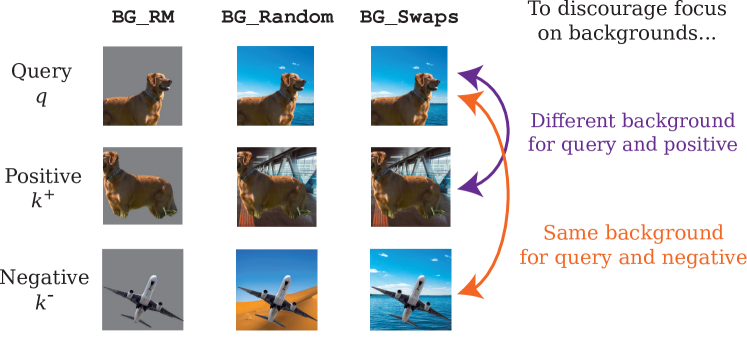
Figure 2: Schematic of different types of background augmentations. BG_RM (left) replaces backgrounds with grayscale, effectively removing any background information. BG_Random (middle) replaces backgrounds with random backgrounds, creating a random signal which is uncorrelated with the foreground. BG_Swaps (right) exploits the structure of contrastive learning to ensure that the query and the positive have the same foreground but different backgrounds, while the query and one negative have matched backgrounds. As a result, BG_Swaps makes it so that models are penalized for focusing on the background.

2.2 Background Augmentations

We apply all background augmentations (BG_RM, BG_Random, BG_Swaps) after all other augmentations in the respective augmentation pipeline. However, we note that we observed similar results applying background augmentations before all other augmentations as well (Appendix C.5). While we apply background augmentations to (views of) images, when it is clear from context, we will refer instead to the corresponding embeddings $q,k^{+},k^{-}$. Unless otherwise mentioned, background augmentations are applied independently with a probability $p_{\text{pos}}$ to both $q$ and $k^{+}$ (the positive teaching pair). When a method has explicit negative instances (MoCo-v2), we denote by $p_{\text{neg}}$ the probability of including a negative whose background matches $q$; by default, this is independent of background augmentation in $q$ and $k^{+}$. Values for $p_{\text{pos}}$ and $p_{\text{neg}}$ were optimized independently for each background augmentation. When it is clear from context, we will sometimes drop the subscript. Note that in MoCo-v2, $k^{+}$ is placed in the queue $Q$ for use in subsequent batches as a negative, so that augmentations applied to $k^{+}$, also indirectly apply to $k^{-}$ via $Q$. When multi-crop augmentation is used (as in SwAV), we apply background augmentations only to the global views. Background augmentations are only applied during self-supervised pre-training and are not applied when training linear classification layers for evaluation. Below, we describe the details of each of the background augmentations we study.

In BG_RM, the background of an image is removed by using a foreground mask (obtained using a saliency detector, see Section 3), and replaced with a solid grayscale background whose intensity is drawn uniformly from $[0,1]$, though we note that a solid black background produced similar results. See illustrative examples in Figure 2, left column.

In BG_Random, we replace the background with a background from a different image in the same batch. As in Xiao et al. (2021a), tiled backgrounds corresponding to an image are generated by filling in the foreground information using the surrounding background.

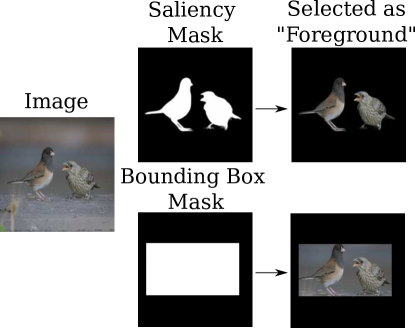
Figure A7: Mask Distortion: Bounding-Box Mask. An example of a bounding-box mask.

In BG_Swaps, we generate a negative image with a background matched to that of the query $q$. In practice, we create a background matched negative as $m_{q}r+(1-m_{q})q$, where $m_{q}$ is the binary foreground mask of the query $q$ and $r$ is a random image. We generate all foreground masks and tiled backgrounds offline and cache them to increase throughput at train time. Note that foreground masks may include multiple foreground objects when they are present (e.g. last row of Figure 3 or Figure A7). Substantial noise is tolerable in the quality of the foreground masks (see Appendix B). More generally, there is substantial flexibility and tolerance in instantiating the main ingredients of background augmentations, which we expand on in Appendix C.

2.3 Supervised Training

We largely follow the protocol from Goyal et al. (2018), unless otherwise indicated. We train all supervised models (with or without background augmentation) with a batch size of 4096 with a 5 epoch linear warmup due to the large batchsize. Models are trained for 90 epochs, with a step schedule (30, 60, 80) and a decay factor of 0.1, using SGD with a base learning rate of 0.1 scaled linearly ($lr$=BatchSize/256$\times 0.1$) and momentum of 0.9, and the standard augmentations RandomResizedCrop and RandomHorizontalFlip. We also exclude bias and batch normalization parameters from weight decay, which was set to $1\times 10^{-4}$. The $\gamma$ in each residual block’s last BatchNorm layer is zero initialized. Our supervised baseline for ResNet-50 reaches the standard baseline (Goyal et al., 2018) performance of $\sim$76.4% Top-1 accuracy on ImageNet (Russakovsky et al., 2015).

3 Saliency Detection

We use saliency detection to generate the foreground masks used in background augmentations (see methods, Section 2.2). However, state-of-the-art saliency detection methods (e.g. U²Net, Qin et al. (2020)) are generally reliant on manually annotated, accurate pixel-level Ground Truth (GT) saliency labels for training, making their usage inappropriate in a truly self-supervised benchmark.

3.1 Weakly Supervised Saliency Detection

Recent “unsupervised” saliency detection methods (Nguyen et al., 2019; Zhang et al., 2018b, 2017a) demonstrate promising results by leveraging psuedo-labels generated by hand-crafted saliency methods in lieu of manually annotated GT saliency labels. Briefly, noisy psuedo-labels generated by hand-crafted saliency methods are iteratively refined by using them as targets to train a Fully Convolutional Network (FCN) for saliency detection, and obtaining refined pseudo-labels from the denoised predictions. Refined pseudo-labels from multiple hand-crafted methods are then jointly used to train a re-initialized FCN to obtain the final saliency detector. While these methods are “unsupervised” in that they do not use manually annotated saliency labels, their success implicitly relies on human annotation—the FCN used is pre-trained in a supervised manner using ImageNet class and CityScapes (Cordts et al., 2016) segmentation labels. Indeed, we find that if we use a randomly initialized FCN instead, the resulting saliency predictions are worse than the noisy psuedo-labels used as targets. As such, these methods are also not appropriate to generate foreground masks for our purpose; we thus refer to these methods as weakly supervised methods in this context.

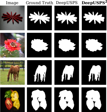
Figure 3: Examples of saliency masks generated by DeepUSPS².

Method	MSRA-B		ECSSD		DUT
	F$\uparrow$	MAE$\downarrow$	F$\uparrow$	MAE$\downarrow$	F$\uparrow$	MAE$\downarrow$
Supervised (GT saliency labels used for training.)
Hou et al. (2017)	89.4	4.7	88.0	7.0	72.9	7.6
Luo et al. (2017)	89.7	4.8	89.1	6.6	73.6	8.0
Zhang et al. (2017b)	-	-	88.3	6.1	69.3	9.8
Zhang et al. (2017c)	-	-	85.2	8.0	66.0	13.2
Wang et al. (2017b)	85.1	6.7	82.6	9.2	67.2	8.5
Li et al. (2016)	-	-	75.9	16.0	60.5	7.6
Wang et al. (2016)	-	-	84.3	9.7	69.2	9.5
Weakly Supervised (Class labels used in pre-trained backbone, GT saliency labels not used in training.)
SBF (Zhang et al., 2017a)	-	-	78.7	8.5	58.3	13.5
USD (Zhang et al., 2018b)	87.7	5.6	87.8	7.0	71.6	8.6
DeepUSPS	90.3	4.0	87.4	6.3	73.6	6.3
DeepUSPS (repro.)	90.5$\pm$0.1	3.9$\pm$0.0	87.9$\pm$0.1	6.3$\pm$0.0	72.1$\pm$0.2	6.8$\pm$0.1
Completely Unsupervised (No human annotation at any stage in the pipeline.)
DeepUSPS2 (ours)	91.3$\pm$0.0	3.6$\pm$0.0	90.0$\pm$0.0	5.4$\pm$0.0	71.1$\pm$0.0	6.9$\pm$0.0

Table 1: DeepUSPS² is on par with or outperforms weakly supervised saliency methods and several recent supervised saliency methods. We report performance across 5 independent runs for DeepUSPS² (and also for DeepUSPS (repro.)). Notation: Mean$\pm$SEM (Standard Error of the Mean). Best results are in bold.

3.2 Unsupervised Saliency Detection: DeepUSPS²

In order to train a completely unsupervised saliency detector, we build upon DeepUSPS (Nguyen et al., 2019), a recent state-of-the-art weakly supervised saliency detection method. We first pre-train a DRN-D-105 (Yu et al., 2017) network in a self-supervised manner for 500 epochs on ImageNet, using BYOL. We then use this pre-trained network to refine pseudo-labels and train a saliency detector, which we call DeepUSPS², employing a training protocol modified from DeepUSPS (see Appendix A.2); some example saliency predictions are shown in Figure 3. Training images were 2500 images from the MSRA-B data set (Liu et al., 2011).

We find that DeepUSPS² performs better than or on par with DeepUSPS and other recent state-of-the-art weakly supervised and even some supervised saliency detectors on common saliency benchmark data sets MSRA-B, ECSSD (Yan et al., 2013), and DUT (Yan et al., 2013), yet DeepUSPS² does not rely on any human annotation at any stage in the pipeline, see Table 1. For each data set, following common protocol (Nguyen et al., 2019; Achanta et al., 2009), we report the F-score,

$$F_{\beta}=\frac{(1+\beta^{2})\times\text{precision}\times\text{recall}}{\beta^{2}\times\text{precision}+\text{recall}},$$

where $\beta^{2}=0.3$ to weigh precision more than recall and the MAE (Mean Absolute Error) on the test split.

We use DeepUSPS² as the default saliency detector to generate foreground masks in our experiments unless otherwise indicated. To ablate the method of mask generation and for control experiments, we also use U²Net (Qin et al., 2020), a state-of-the-art saliency detector that is trained in a supervised manner on DUTS-TR (Wang et al., 2017a), which contains 10553 pixel-level manual saliency annotations.

4 Representation Learning with Background Augmentations

Method	Epochs	ImageNet acc.
		Original	ReaL
Supervised	90	76.4	82.7
PCL-v2 (Li et al., 2021b)	200	67.6	-
CMC (Tian et al., 2020a)	200	66.2	-
SimCLR	200	66.8	-
MoCo	200	60.6	-
SeLa (Asano et al., 2020)	400	61.5	-
MoCo-v2	200	67.5	-
MoCo-v2 (repro.)	220	67.7	74.7
MoCo-v2 + BG_RM	220	69.1$\pm$0.0 (+1.4)	76.2$\pm$0.0 (+1.5)
MoCo-v2 + BG_Swaps	220	69.5$\pm$0.1 (+1.8)	76.6$\pm$0.1 (+1.9)
DiLo (MoCo-v2) (Zhao et al., 2021)	200	67.9 (+0.2)	-
BYOL	300	72.5	-
BYOL (repro.)	300	72.7	79.6
BYOL + BG_RM	300	73.3$\pm$0.2 (+0.6)	80.4$\pm$0.3 (+0.8)
BYOL + BG_Random	300	73.9$\pm$0.1 (+1.2)	81.0$\pm$0.0 (+1.4)
SwAV	100	72.1	-
SwAV (repro.)	100	72.2	79.1
SwAV + BG_RM	100	73.6$\pm$0.1 (+1.4)	80.6$\pm$0.1 (+1.5)
SwAV + BG_Random	100	73.4$\pm$0.0 (+1.2)	80.4$\pm$0.1 (+1.3)
Longer Training
PIRL (Misra and van der Maaten, 2020)	800	63.6	-
SimCLR	1000	69.3	-
Barlow Twins (Zbontar et al., 2021)	1000	73.2	-
MoCo-v2	800	71.1	-
MoCo-v2 (repro.)	800	71.0	78.0
MoCo-v2 + BG_RM	800	71.9 (+0.9)	78.9 (+0.9)
MoCo-v2 + BG_Swaps	800	72.2 (+1.2)	79.2 (+1.2)
BYOL	1000	74.3	-
BYOL (repro.)	1000	73.8	80.5
BYOL + BG_RM	1000	74.6 (+0.8)	81.3 (+0.8)
BYOL + BG_Random	1000	74.8 (+1.0)	81.7 (+1.2)
SwAV	800	75.3	-
SwAV (repro.)	800	74.9	81.4
SwAV + BG_RM	800	76.1 (+1.2)	82.5 (+1.1)
SwAV + BG_Random	800	76.1 (+1.2)	82.6 (+1.2)

Table 2: Background augmentations confer large performance benefits in linear evaluation on ImageNet across a spectrum of SSL methods using the original or reassessed labels. For shorter training, we report metrics averaged over 3 independent runs, reflecting robust improvements. Number of training epochs are chosen to be consistent with previously published results. We highlight performance gains due to background augmentations relative to our reproductions, but also include published baseline numbers for comparison. Notation: Mean$\pm$SEM (Standard Error of the Mean). Best results are in bold.

4.1 Do Background Augmentations that Encourage Semantic Focus Increase Performance?

Deep neural networks often rely on non-semantic, superficial features and thus may be easily misled by backgrounds. Nonetheless, these non-semantic features are often predictive at test time (Xiao et al., 2021a; Sehwag et al., 2020; Ilyas et al., 2019), so it is not a priori obvious whether background augmentations that encourage semantic focus on the foreground will benefit performance. We investigate this question by exploring the space of possible background augmentations. First, we study removing backgrounds probabilistically, where the strength of the augmentation is controlled by a parameter $p$, which sets the probability that the background is removed from the query or positive key. See Figure 2, left for an example of the BG_RM setting.

Across SSL methods, we find that BG_RM substantially improves linear classification on ImageNet, improving performance by $\sim$0.6-1.4% (Table 2). For all methods, we found that a moderate value of $p$ between 0.1 and 0.3 is generally a good setting. However, despite its improved performance, because BG_RM introduces images with solid gray backgrounds, it induces a distribution shift between the unsupervised pre-training phase and the supervised downstream tasks which may limit performance improvements. Note that DiLo (MoCo-v2) is similar to BG_RM applied MoCo-v2, but results only in a small gain of +0.2, while we obtain a 7$\times$ larger gain (and as we will show later, a 9$\times$ gain by developing an improved background augmentation method BG_Swaps).

4.2 Can we make Background Augmentations more In-Distribution?

In the previous section, we explored removing backgrounds and replacing them with uniform grayscale, which results in the data being out-of-distribution (OOD) relative to the downstream tasks. To mitigate this OOD issue, we instead replace backgrounds with a randomly chosen background from another instance in the same batch. We term this method BG_Random (Figure 2, middle). Interestingly, despite the fact that BG_Random is more in-distribution than BG_RM, we found that performance was similar (e.g. 69.1% for BG_RM (Table 2) vs. 69.2% for BG_Random (Table A6) with MoCo-v2). However, we note that these two settings are not necessarily directly comparable. For example, in the case of MoCo-v2, augmented positive keys are added to the queue to be used as negatives for subsequent mini-batches. As a result, BG_RM might actually penalize background focus whereas BG_Random may simply result in an uninformative background. This is because BG_RM features a constant gray background which can be matched between the query and negatives that were used as positive keys in a previous mini-batch, whereas BG_Random features distinct backgrounds for each augmented image.

	Method	BG aug. in			ImageNet acc.
		$q$	$k^{+}$	$k^{-}$
(a)	baseline				67.7
Control Experiments
(b)	BG_RM	✓			67.8
(c)	BG_Random	✓			68.3
“Full” Augmentations
(d)	BG_RM	✓	✓	✓	69.3
(e)	BG_Random	✓	✓		69.1

Table 3: BG_RM vs. BG_Random. Comparing BG_RM and BG_Random in MoCo-v2 controlling for presence of negatives in the queue with similar background.

It is therefore unclear whether the similar performance of BG_RM and BG_Random stems from distributional shift or the matched gray backgrounds which can serve to make negatives more challenging. To disentangle these two factors, we performed a control experiment in which background augmented images were only included for the query (with $p=0.1$)—and thus not used in subsequent mini-batches as the positive or the negative. This setting maintains the distribution shift of BG_RM, but removes the possibility of a teaching signal originating from matched gray backgrounds across the query and negative. To minimize confound stemming from mask quality, we use higher quality foreground masks generated by U²Net, a state-of-the-art saliency detector trained with supervision instead of DeepUSPS².

This control reveals that, when only applied to the query but not the positive or negative, BG_RM has similar performance (Table 3b) as no BG_RM (Table 3a), suggesting that BG_RM benefits substantially from the teaching signal of negatives with matching (constant) backgrounds. In contrast, we found that, when only present in the query, BG_Random still improves performance (Table 3c), but the improvement is decreased suggesting that having augmented images with randomized backgrounds in the positive keys provides additional benefit (Table 3e); here, for an apples-to-apples comparison with the control experiments (or “partial” augmentations), we also report performance for the “full” augmentations (Table 3d, e) using U²Net masks and the same augmentation strength.

These analyses demonstrate both the importance of using background augmentations which remain close to the unaugmented input distribution and highlight the potential for methods which provide an additional teaching signal via negatives with query-matched backgrounds. Inspired by these results, we next investigate how to combine these approaches.

4.3 Exploiting the Structure of Contrastive Instance Discrimination via Background Matched Negatives

	Method	BG aug. in			ImageNet acc.
		$q$	$k^{+}$	$k^{-}$
(a)	baseline				67.7
(b)		✓			68.3
(c)			✓		68.2
(d)	BG_Random	✓	✓		69.1
(e)	BG_Swaps	✓	✓	✓	69.7

Table 4: Ablations of BG_Swaps for MoCo-v2. Each component confers a performance improvement and the improvements stack on top of each other.

Thus far, we have explored two background augmentations—BG_RM  and BG_Random—both of which operate independently on the query and the positive and encourage semantic focus on foregrounds by simply removing backgrounds altogether or replacing them with randomized backgrounds so there’s no effective signal in the background. This removes the incentive for models to focus on background information, but does nothing to directly penalize focus on backgrounds. However, contrastive instance discrimination (CID) methods (e.g., MoCo, SimCLR), use the query to discriminate between the positive and negative instances and thus feature structure that we can exploit to not only remove signal from backgrounds, but go further and provide explicitly misleading signal in the backgrounds. Note that BYOL and SwAV are not CID methods, since they do not use negative instances.

We accomplish this through two modifications with a method we call BG_Swaps (Figure 2, right). First, as in BG_Random, we ensure that the query and the positive feature distinct random backgrounds. Models which focus on backgrounds would therefore place the positive and query further apart than they should since the semantic content is identical, but the background features differ. Second, we modify the negative set to include one additional negative whose background matches the query: a network which focuses on backgrounds would view the background-matched negative as highly similar to the query and receive strong negative supervision. As with BG_RM and BG_Random, we introduce the background-matched negative with probability $p_{\text{neg}}$ (and include a randomly selected negative with probability $1-p_{\text{neg}}$, so that the total number of negatives is always $|Q|+1$).

These background matched negatives can be considered an example of “hard negatives”, which have been explored recently in the context of SSL to improve learning (Kalantidis et al., 2020; Wu et al., 2021; Robinson et al., 2021; Cai et al., 2020). In this vein, one could consider the positive pair ($q$ and $k^{+}$) with different backgrounds as “hard positives”. For MoCo-v2, including a background matched negative further increases performance over BG_RM by an additional 0.4% (Table 2). Consistent with our previous findings, we also found that it is important for the statistics of the augmentations to be similar for the positive and the negatives in order to achieve the best performance. In general, we found that the probability of an augmentation in the query and positive, $p_{\text{pos}}$, matching the probability of an augmentation in the negative, $p_{\text{neg}}$, so that $p_{\text{pos}}$$\simeq$$p_{\text{neg}}$, gives good performance.

4.4 Ablating BG_Swaps

To characterize which components of the BG_Swaps augmentation matter and how much, we perform systematic ablations. As shown in Table 4, we found that each independent component of BG_Swaps leads to a performance improvement (in contrast with BG_RM). In particular, we find benefits when employing each of the following: BG_Random in the query ($p=0.1$); BG_Random in the positive key ($p=0.1$); background matched negative ($p=0.2$). Notably, the improvements from randomized backgrounds in $q$ and $k^{+}$ stack superlinearly (Table 4d), suggesting that incorporating both of these augmentations provides a greater advantage due to their interaction than either does independently; using background matched negatives further improves performance substantially (Table 4e). As in the control experiments in Section 4.2, to minimize confound stemming from mask quality, we use higher quality foreground masks generated by U²Net for these ablations.

There is significant design flexibility in how one could implement BG_Swaps. For example, is it a better teaching signal to have independent or correlated background augmentations in the query/positive and the negatives? Is it better to have a negative whose background matches the query or the positive? We find that BG_Swaps is robust to these specific choices (Appendix C), making it a promising candidate for more general deployment in augmentation pipelines.

4.5 Effect of Longer Training

We also evaluate the impact of background augmentations on longer training ranging from 800 to 1000 epochs (Table 2). As with the shorter training, we found that background augmentations consistently increased performance across models, e.g. enabling SwAV to reach 76.1% with a ResNet-50 on ImageNet, only 0.3% less than the standard supervised baseline. Interestingly, however, we found that the magnitude of the improvement decreased slightly in the longer training runs, which may be a saturation effect but also raises the more interesting possibility that SSL models initially learn representations that depend on backgrounds, but eventually learn some background invariance when trained for long enough. However, we later discuss (Section 5.1) evidence that does not find support for the latter possibility.

4.6 Diagnosing and Improving SwAV + Background Augmentations

SwAV w/ wider MLP (4096/256)
Epochs	baseline	BG_RM	BG_Random
100	72.6	74.1	74.1
800	75.0	76.1	76.1

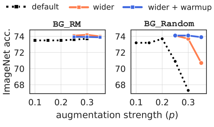
Figure 4: Wider projection MLP and warmup alleviates early optimization difficulty. (left) Wider projection MLP alleviates early optimization difficulty, improving performance and removes the gap between BG_RM and BG_Random. Augmentation strength: $p=0.25$. (right) The gap between BG_RM and BG_Random increases with stronger augmentation with the default (black dashed lines) MLP capacity. In addition to increasing MLP capacity, warming up background augmentations further adds stability across a range of augmentation strengths. Notation: (MLP width/output dimension).

As previously discussed, due to BG_RM being OOD, we might generally expect BG_Random, BG_Swaps to be on par or better than BG_RM. Our results in Table 2 show that while this is generally true across SSL methods and training durations, BG_RM $>$ BG_Random for SwAV trained for a short duration. Since BG_RM and BG_Random result in the same final accuracy upon longer training (Table 2), we hypothesized that there maybe early optimization difficulty arising from an interaction between SwAV’s objective function and attempting to learning invariance to random natural backgrounds (in contrast with solid grayscale backgrounds in BG_RM), at a stage in the pre-training when the representations are still quite poor. Consistent with this hypothesis, when BG_Random is used, the loss lingers at chance early in pre-training, while the corresponding loss for BG_RM falls rapidly. We reasoned that further increasing the augmentation strength of BG_Random should result in higher optimization difficulty and consequently, worse performance. Consistent with this expectation, the performance of BG_Random rapidly declines past a point, while the performance of BG_RM remains stable, see Figure 4 (right, black dashed lines).

To alleviate this issue, we propose two solutions: a) increasing the projection MLP capacity and b) warming up background augmentations. We show results from (a) in Figure 4 (left, Table), finding both improved performance (a baseline effect) and removing the gap between BG_RM and BG_Random. Note that the default projection MLP capacity for SwAV is 2048/128. We report the results of (a) and (b) across a range of augmentation strengths in Figure 4 (right) . In addition to increasing MLP capacity, warming up BG_Random further stabilizes performance when stronger augmentation is used. More broadly, these analyses show that additional factors such as ease of optimization play an important role in determining performance apart from whether an augmentation induces a distribution shift.

Our analyses here have broader implications. For instance, they shed new light on the role of the projection MLP and may help explain recent puzzling findings in literature; specifically, Zbontar et al. (2021) observed that their method, Barlow Twins, works best for large dimensionality of the projection MLP and noted that “This result is quite surprising because the output…acts as a dimensionality bottleneck in our model and sets the limit of the intrinsic dimensionality of the representation”. Our analyses suggest that it is important for the projection MLP to be of appropriate capacity for the pretext prediction task—more “difficult” (e.g. due to stronger augmentation) prediction losses may benefit from a higher capacity MLP.

Method	Saliency	ImageNet acc.
	Method	Original		ReaL
		Top-1	Top-5	Top-1	Top-5
MoCo-v2 (220)		67.7	88.1	74.7	91.7
+ BG_RM	DeepUSPS2	69.1$\pm$0.0 (+1.4)	88.8$\pm$0.0	76.2$\pm$0.0 (+1.5)	92.3$\pm$0.1
	U2Net	69.3$\pm$0.1 (+1.6)	88.6$\pm$0.1	76.3$\pm$0.1 (+1.6)	92.3$\pm$0.1
+ BG_Swaps	DeepUSPS2	69.5$\pm$0.1 (+1.8)	88.9$\pm$0.0	76.6$\pm$0.1 (+1.9)	92.4$\pm$0.1
	U2Net	69.7$\pm$0.1 (+2.0)	88.9$\pm$0.0	76.8$\pm$0.1 (+2.1)	92.3$\pm$0.1
BYOL (300)		72.7	90.9	79.6	94.0
+ BG_RM	DeepUSPS2	73.3$\pm$0.2 (+0.6)	91.1$\pm$0.1	80.4$\pm$0.3 (+0.8)	94.3$\pm$0.1
	U2Net	73.5$\pm$0.1 (+0.8)	91.2$\pm$0.1	80.5$\pm$0.1 (+0.9)	94.4$\pm$0.0
+ BG_Random	DeepUSPS2	73.9$\pm$0.1 (+1.2)	91.6$\pm$0.0	81.0$\pm$0.0 (+1.4)	94.6$\pm$0.0
	U2Net	73.8$\pm$0.0 (+1.1)	91.7$\pm$0.0	81.0$\pm$0.1 (+1.4)	94.7$\pm$0.0
SwAV (100)		72.2	91.0	79.1	94.0
+ BG_RM	DeepUSPS2	73.6$\pm$0.1 (+1.4)	91.6$\pm$0.0	80.6$\pm$0.1 (+1.5)	94.6$\pm$0.0
	U2Net	73.7$\pm$0.1 (+1.5)	91.6$\pm$0.0	80.7$\pm$0.1 (+1.6)	94.6$\pm$0.0
+ BG_Random	DeepUSPS2	73.4$\pm$0.0 (+1.2)	91.6$\pm$0.0	80.4$\pm$0.1 (+1.3)	94.6$\pm$0.0
	U2Net	73.5$\pm$0.1 (+1.3)	91.6$\pm$0.0	80.5$\pm$0.1 (+1.4)	94.6$\pm$0.0
Longer Training
MoCo-v2 (800)		71.0	90.3	78.0	93.4
+ BG_RM	DeepUSPS2	71.9 (+0.9)	90.4	78.9 (+0.9)	93.5
	U2Net	72.0 (+1.0)	90.4	79.0 (+1.0)	93.6
+ BG_Swaps	DeepUSPS2	72.2 (+1.2)	90.4	79.2 (+1.2)	93.6
	U2Net	72.2 (+1.2)	90.5	79.0 (+1.0)	93.5
BYOL (1000)		73.8	91.5	80.5	94.3
+ BG_RM	DeepUSPS2	74.6 (+0.8)	91.8	81.3 (+0.8)	94.7
	U2Net	74.7 (+0.9)	91.9	81.5 (+1.0)	94.7
+ BG_Random	DeepUSPS2	74.8 (+1.0)	92.0	81.7 (+1.2)	94.8
	U2Net	74.8 (+1.0)	92.1	81.6 (+1.1)	94.8
SwAV (800)		74.9	92.1	81.4	95.1
+ BG_RM	DeepUSPS2	76.1 (+1.2)	92.8	82.5 (+1.1)	95.4
	U2Net	76.2 (+1.3)	92.8	82.6 (+1.2)	95.4
+ BG_Random	DeepUSPS2	76.1 (+1.2)	92.9	82.6 (+1.2)	95.5
	U2Net	76.0 (+1.1)	92.9	82.6 (+1.2)	95.5

Table 5: Ablating the impact of the saliency method used for foreground extraction. We find nearly identical performance when we use U²Net, a state-of-the art saliency detector that is trained with supervision. Foreground extraction using higher quality masks results in slightly better performance when trained for fewer epochs, but this benefit disappears with longer training. All numbers are based on our implementation. Notation: MoCo-v2 (800) indicates that MoCo-v2 was trained for 800 epochs.

One important limitation of current SSL methods is the long training required for competitive performance, typically 800-1000 epochs, in contrast with supervised learning. Our results in Figure 4 (left) show that background augmentations enable a step forward in reducing the amount of training required for competitive performance in SSL. In these results, aside from diagnosing and fixing early optimization issues, we simply used the default settings for SwAV. However, there remains much room for improvement in conjunction with background augmentations. We briefly explore one such improvement here.

Recall that SwAV uses multi-crop augmentation, where local crops covering small parts of the image are expected to be predictive of global crops. Here, we increase the area that the small crops may cover of the full image . While the small crops may feature more of the background with this change, background augmentations already prevent excessive focus on the background. This simple change improves the performance of BG_RM (BG_Random) from 74.1% to 74.4% (74.2%). In only 100 epochs, performance exceeds many recent high performing SSL methods trained for 800-1000 epochs, e.g. Barlow Twins (73.2%, 1000 epochs), MoCo-v3 (Chen et al., 2021) (73.8%, 800 epochs) and BYOL (74.3%, 1000 epochs). In contrast, with the same change, the SwAV baseline fails to train and the loss at the end of pre-training is at chance. Note that our default setting for SwAV does not include the modifications discussed in this section unless otherwise indicated.

4.7 What is the Impact of Mask Quality?

While DeepUSPS² is better than or on par with weakly supervised saliency methods and even some recent supervised saliency methods, state-of-the-art supervised saliency methods like U²Net achieve better performance on saliency benchmarks. We perform an ablation using foreground masks generated by U²Net for background augmentations. While the resulting models are not truly self supervised, they can nevertheless help us understand if using better foreground masks can lead to larger performance improvements. We report the results of these experiments in Table 5, finding that performance is nearly identical whether DeepUSPS² or U²Net are used to extract foreground masks. Using higher quality masks leads to slightly better performance when trained for fewer epochs but this gap disappears with longer training. In later sections, we evaluate both sets of models on a range of downstream tasks to gain further insight.

While these results suggest that there may be diminishing gains to using higher quality masks, some natural questions arise, e.g. which SSL methods and background augmentations are more robust to mask quality? How does performance vary as a function of mask quality? We systematically perturb mask quality in numerous ways (via mask rotation, shearing, translation, flips and replacing masks with bounding-box masks) to answer these questions in Appendix B. Overall, we find that there is substantial robustness to mask quality. Of the SSL methods and background augmentations considered, we find that SwAV and BG_Swaps are particularly robust.

4.8 Limited-Label Setting

While linear evaluation using 100% of ImageNet labels is a standard evaluation metric, it is also somewhat impractical due to the large amount of labels involved - after all, one of the more important goals of SSL is good performance when labeled data is highly limited. Linear evaluation in limited label settings reveals a large improvement in performance from background augmentations. For 1% and 10% labels, we use the same fixed splits of ImageNet labeled training data as in Chen et al. (2020b). We similarly find large performance benefits in semi-supervised evaluation (fine-tuning the pre-trained backbone in addition to learning a linear classifier). We report Top-1 and Top-5 accuracies in Table 6.

Method		1% Labels		10% Labels
		Top-1	Top-5	Top-1	Top-5
Supervised (Zhai et al., 2019)		25.4	48.4	56.4	80.4
Linear	MoCo-v2 (repro.)	52.0	77.7	63.9	85.8
	MoCo-v2 + BG_RM	54.1 (+2.1)	78.6	65.1 (+1.2)	86.2
	MoCo-v2 + BG_Swaps	56.0 (+4.0)	79.5	65.9 (+2.0)	86.4
	BYOL (repro.)	57.5	80.8	68.6	88.6
	BYOL + BG_RM	60.1 (+2.6)	82.7	70.1 (+1.5)	89.2
	BYOL + BG_Random	60.9 (+3.4)	83.3	70.4 (+1.8)	89.5
	SwAV (repro.)	52.8	78.4	68.3	88.7
	SwAV + BG_RM	57.0 (+4.2)	81.3	70.4 (+2.1)	89.8
	SwAV + BG_Random	56.4 (+3.6)	81.1	70.2 (+1.9)	89.7
Finetune	MoCo-v2 (repro.)	54.1	81.3	67.6	89.4
	MoCo-v2 + BG_RM	55.2 (+1.1)	81.3	67.8 (+0.2)	89.2
	MoCo-v2 + BG_Swaps	57.3 (+3.2)	82.4	68.7 (+1.1)	89.5
	BYOL (repro.)	57.3	80.5	70.6	90.0
	BYOL + BG_RM	59.9 (+2.6)	82.4	71.7 (+1.1)	90.5
	BYOL + BG_Random	60.7 (+3.4)	82.8	72.0 (+1.4)	90.7
	SwAV (repro.)	54.0	78.5	70.1	89.9
	SwAV + BG_RM	55.2 (+1.2)	79.4	70.8 (+0.7)	90.2
	SwAV + BG_Random	55.9 (+1.9)	79.4	71.1 (+1.0)	90.4
	Published Baselines
	PIRL	-	57.2	-	83.8
	SimCLR	48.3	75.5	65.6	87.8
	SwAV	53.9	78.5	70.2	89.9
	BYOL	53.2	78.4	68.8	89.0
	Barlow Twins	55.0	79.2	69.7	89.3

Table 6: Limited-Labels Setting. Background augmentations improve performance in the limited-labels setting. Linear evaluation using 100% of ImageNet labels though a standard benchmark, is a somewhat unrealistic setting. Evaluation in the more practical setting of limited-labels reveals even larger improvement in performance. We highlight performance gains due to background augmentations. Best (second best) results are in bold (underlined).

Our first key finding is that the improvement in performance in limited label settings, for both linear and semi-supervised evaluation, is substantially larger than in 100% linear evaluation, with improvements up to 4.2%. Large gains in linear evaluation especially reflect a much better learned representation, since the backbone is frozen. Our second key finding is that BG_Swaps is especially effective in limited label settings. Indeed, in the 1% setting, the gain from BG_Swaps is nearly $3\times$ the gain from BG_RM in semi-supervised evaluation and $\sim 2\times$ that of BG_RM in linear evaluation, demonstrating the effectiveness of using negatives matched to the query’s background.

Our third finding is that it is generally better to use BG_Random or BG_Swaps over BG_RM, consistent with our previous results. Our findings here set new, stronger baselines: 60.9% Top-1 in the 1% labels setting and 72% Top-1 in the 10% labels setting. It is worth noting that $\sim$71% is the linear evaluation baseline for MoCo-v2  using 100% of the labels. Note that our reproduction of BYOL’s performance in limited label settings already improves upon the published baseline (by +4.1%, +1.8% in the 1% and 10% labels settings respectively) by adopting a much smaller learning rate for the pre-trained backbone than the classifier head—background augmentations further improve on these stronger baselines.

Finally, we note that nearly identical findings hold when we instead use U²Net for foreground extraction, see Table A13. All models receive full pre-training.

4.9 Can Background Augmentations Improve Performance in the Supervised Setting?

We have found that background augmentations provide a significant performance boost to a suite of high-performing SSL methods, and shrink the gap to the supervised baseline down to $0.3\%$. We note that most SSL methods utilize an augmentation suite that is inherited from supervised training. By designing augmentations specifically for SSL, we were able to induce a substantial increase in performance; this raises the question of whether a similar performance boost would be observed when applying background augmentations to supervised training.

baseline ($p=0.0$): 76.4	$p=0.1$	$p=0.2$	$p=0.3$	$p=0.5$
BG_RM	76.6	76.5	76.4	75.9
BG_RM + retrain classifier	76.5	76.3	76.0	75.1
BG_RM + finetune	76.5	76.6	76.5	76.0
BG_Random	76.4	76.6	76.6	76.0
BG_Random + retrain classifier	76.4	76.2	75.9	73.5
BG_Random + finetune	76.6	76.6	76.6	76.4

Table 7: Supervised Setting: Background augmentations do not improve over the baseline (76.4 in our setting).

Interestingly, we find that background augmentations do not confer a performance benefit in the supervised setting. In Table 7, we report the performance of BG_RM and BG_Random, sweeping over $p$, finding no setting that outperforms the supervised benchmark.

Method	Epochs	Accuracy
Supervised baseline	90	76.4
Supervised + BG_RM	90	76.5
Supervised + BG_RM	300	76.5
Supervised + BG_Random	90	76.6
Supervised + BG_Random	300	76.6

Table 8: Supervised Setting: Longer Training. Longer training with background augmentation does not significantly improve performance in the supervised setting over the baseline. Augmentation strength: $p=0.2$.

One may wonder if this lack of improvement is an artifact of the evaluation protocol, which is different from the SSL setting, where evaluation is either by training a linear classifier on top of the frozen trunk or by fine-tuning the whole network (trunk + linear classifier) without background augmentations. We therefore, a) re-train a linear classifier without background augmentations on top of the frozen trunk (of the supervised network trained with background augmentations) and (separately) b) fine-tune the whole network without background augmentations, once again finding no performance benefit.

In the supervised setting, strong augmentations may require much longer training to be effective (e.g. as in the case of CutMix (Yun et al., 2019)). To account for a similar possibility in the case of background augmentations, we include background augmentations in supervised training and follow a much longer training schedule (see Appendix A for details) for 300 epochs (following CutMix) and find no significant performance benefits, see Table 8.

4.10 So, When do Background Augmentations Help?

Our results in the previous section suggest that the utility of background augmentations in SSL does not generalize to the supervised setting. Given the importance of augmentations to SSL (e.g., Chen et al. (2020a)), these results highlight the need to evaluate and explore augmentations tailor-made for the SSL setting and are consistent with similar findings (Chen et al., 2020a) for color distortion and blur augmentations. While the test bed of high performing SSL methods we have considered thus far is diverse, they share a commonality: they all use Siamese networks to compare or contrast views of images, raising the natural question of whether this is the only SSL setting where background augmentations confer an advantage.

baseline $(p=0.0)$: 36.1	$p=0.1$	$p=0.2$	$p=0.3$	$p=0.5$
BG_RM	36.0	35.5	35.5	34.8
BG_Random	36.1	36.0	35.9	35.7

Table 9: RotNet: Background augmentations do not improve over the baseline.

To investigate this question, we turn to RotNet (Gidaris et al., 2018)—a simple, yet surprisingly effective SSL method that is not based on a Siamese architecture nor on comparisons between images. Training a RotNet involves augmenting the data with rotated images and training a network to categorize the orientation of an image, thereby forcing the network to learn a meaningful representation to accomplish this task. We implemented background augmentations in RotNet, i.e. we either perform BG_RM or BG_Random followed by rotating the image (and training the network to classify the orientation). Interestingly, we found that background augmentations confer no performance benefits, see Table 9. Here, BG_Random and BG_RM decorrelate the foreground and the background, while BG_RM additionally reduces the incentive to encode background information, since a grayscale background is not informative for the pretext task of categorizing image orientation. Thus, merely decorrelating the foreground and background or disincentivizing focus on the background are not sufficient to improve semantic focus.

Based on our findings, we speculate that background augmentations are most helpful when there is a similarity comparison between images, and can help prevent the model from using the background as a shortcut to place images nearby (or far away) in embedding space which can hinder learning about the semantic content present in an image.

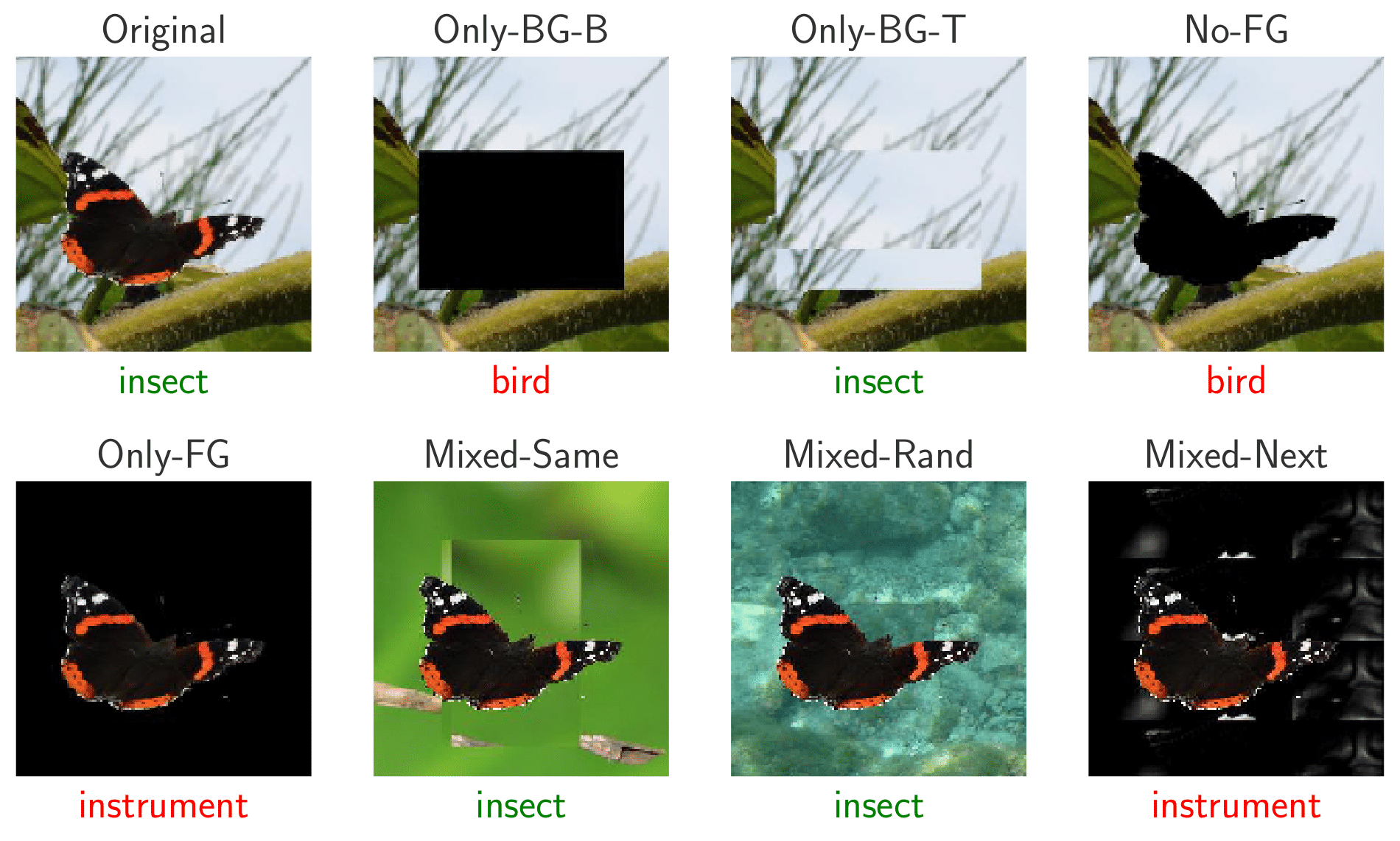
Figure 5: Examples of variations of ImageNet-9. Also shown are classification decisions from the supervised baseline. Image from Xiao et al. (2021a).

5 Generality of Representations Induced by Background Augmentations

If background augmentations lead to increased focus on semantic content and decreased focus on non-robust predictors for classification (e.g., Ilyas et al. (2019)), we expect that these augmentations would also lead to improved performance on out-of-distribution downstream tasks. In particular, we expect gains on those tasks which have proven especially challenging for supervised networks. Here, we discuss several such tasks, including ImageNet-9 (Xiao et al., 2021a), adversarial attacks (Goodfellow et al., 2015; Kurakin et al., 2016; Madry et al., 2018), natural adversarial examples (Hendrycks et al., 2019b), ImageNet-Renditions (Hendrycks et al., 2021) and ReaL ImageNet (Beyer et al., 2020), finding improved performance across the board.

5.1 Improved Robustness to Shift in Foreground-Background Statistics

ImageNet-9 (IN-9), introduced in Xiao et al. (2021a), consists of out-of-distribution data sets that are different variations of a 9-class subset of ImageNet. The variants are designed to have different amounts of foreground and background signal, see Figure 5 for examples. In the Only-BG-B and Only-BG-T variants, the foreground is removed and replaced either with a black box (Only-BG-B) or a tiled version of the background (Only-BG-T); No-FG features images with the foreground shape cut out (and discernible), while Only-FG features the foreground alone on a black background (similar to our BG_RM); Mixed-Same, Mixed-Rand, and Mixed-Next, feature foregrounds pasted onto backgrounds from different images of the same class (Mixed-Same), random images (Mixed-Rand), and deterministically from the next class such that backgrounds provide systematically misleading information (Mixed-Next). If models learn to focus on the semantically meaningful foreground and ignore the background, we should expect classification performance to decrease for Only-BG-B and Only-BG-T, and to increase for Only-FG, Mixed-Same, Mixed-Rand, and Mixed-Next.

Data Set	Supervised	MoCo-v2			BYOL			SwAV
		baseline	BG_RM	BG_Swaps	baseline	BG_RM	BG_Random	baseline	BG_RM	BG_Random
Original	95.6	92.7	93.8	94.2	94.9	95.6	96.0	94.1	95.0	94.9
Only-BG-B $\downarrow$	11.4	6.1	6.1	3.6	5.4	4.9	6.0	10.9	8.8	8.3
Only-BG-T $\downarrow$	16.3	14.8	12.9	9.3	12.7	11.8	11.5	15.8	16.7	17.6
No-FG	45.9	37.8	42.3	39.6	43.9	45.9	46.2	41.3	44.2	45.2
Only-FG $\uparrow$	86.8	74.4	81.9 (+7.5)	86.1 (+11.7)	83.5	88.8 (+5.3)	87.7 (+4.2)	79.4	85.3 (+5.9)	84.3 (+4.9)
Mixed-Same $\uparrow$	86.2	81.8	84.0 (+2.2)	87.9 (+6.1)	86.2	88.6 (+2.4)	90.1 (+3.9)	82.2	86.1 (+3.9)	86.3 (+4.1)
Mixed-Rand $\uparrow$	78.9	70.7	76.3 (+5.6)	84.1 (+13.4)	79.6	83.2 (+3.6)	85.5 (+5.9)	71.3	77.1 (+5.8)	77.0 (+5.7)
Mixed-Next $\uparrow$	77.2	67.0	73.0 (+6.0)	82.2 (+15.2)	77.6	80.7 (+3.1)	84.0 (+6.4)	69.0	74.3 (+5.3)	74.4 (+5.4)

Table 10: Robustness: Foreground-Background Shifts. Background augmentations result in large performance gains on ImageNet-9 across all SSL methods, with BG_Swaps generally exhibiting similar or better performance than BG_RM. We highlight the performance benefit on the variants of ImageNet-9 especially relevant to our work. All accuracies reported for background augmented SSL methods are averages of 3 independent runs (we exclude SEM to avoid clutter, see Table A14 for an expanded table that includes SEM). All pre-training durations correspond to respective medium settings. Note that ImageNet-9 uses only 9 classes, so chance is $\sim$11.1%.

We evaluate the baseline SSL methods as well as models with background augmentations on all variants of IN-9 in Table 10. As in the supervised setting (see Xiao et al., 2021a), we found that models which perform better on the Original IN-9 also perform better across other IN-9 variants. Critically, we also found that background augmentations consistently improved performance on IN-9, especially on the images with misleading backgrounds (Mixed-X), and in some cases, enable outperforming the supervised baseline. We also found that BG_Swaps consistently improved performance over BG_RM. For example, on Mixed-Next, the MoCo-v2 baseline has an accuracy of 67.0%, worse than the supervised baseline’s performance of 77.2%, but incorporating BG_RM and BG_Swaps increases this to 73.0% and 82.2%, respectively. These results demonstrate that background augmentations do indeed encourage semantic focus on the foreground, and that explicitly discouraging background focus (as in BG_Swaps) is beneficial over simply removing positive signal in the background. We also note that BG_Random generally confers larger improvements over BG_RM.

Pre-Train Duration	MoCo-v2			BYOL			SwAV
	baseline	BG_RM	BG_Swaps	baseline	BG_RM	BG_Random	baseline	BG_RM	BG_Random
Med.	11.1	7.7 (-3.4)	3.8 (-7.3)	6.6	5.4 (-1.2)	4.6 (-2.0)	10.9	9.0 (-1.9)	9.3 (-1.6)
Full	10.0	6.8 (-3.2)	4.4 (-5.6)	9.1	5.3 (-3.8)	4.4 (-4.7)	11.4	9.3 (-2.1)	9.0 (-2.4)

Table 11: BG-Gap: Background augmentations decrease BG-Gap of SSL Methods.

To quantify the impact of foreground-background correlations in the learned representations, we compute the BG-Gap (Xiao et al., 2021a) as the difference between accuracies in the Mixed-Same and Mixed-Rand settings and find that background augmentations decrease the BG-Gap in the SSL methods considered, relative to the baselines. For the baselines, we also find that the BG-Gap slightly increases when trained for longer (Table 11) for BYOL and SwAV, while it slightly decreases for MoCo-v2. We speculate that this is due to the use of a large number ($|Q|=65536$) of negative instances in MoCo-v2—it is possible some of the negative instances have backgrounds similar to the query $q$, thereby implicitly discouraging background focus. As such, SSL models do not seem to learn much background invariance when trained for longer duration. When background augmentations are used, the BG-Gap is roughly the same for shorter or longer training duration—in other words, background augmentations do not require long training to be effective. Additional results: Appendix D (Tables A14, A15, A16, A17, A18).

5.2 ReaL Imagenet Confirms Improvement of Semantic Focus

Next, we evaluate performance using Reassessed Labels (ReaL, Beyer et al. (2020)) for ImageNet, which relabel ImageNet to better represent the semantic content of the images. Using ReaL, Beyer et al. (2020) found that the gains due to many recent methods were smaller than when the original labels are used. As with the original ImageNet labels, we found that background augmentations substantially improve performance on ImageNet ReaL (Table 2), confirming that background augmentations do induce increased semantic focus rather than simply facilitating overfitting to the original ImageNet labels. In fact, the improvement on ReaL is slightly larger when trained for fewer epochs.

Pre-Train Duration	MoCo-v2			BYOL			SwAV
	baseline	BG_RM	BG_Swaps	baseline	BG_RM	BG_Random	baseline	BG_RM	BG_Random
Med.	54.7	56.7$\pm$0.1 (+2.0)	57.2$\pm$0.1 (+2.5)	60.7	61.7$\pm$0.2 (+1.0)	62.1$\pm$0.1 (+1.4)	59.3	61.2$\pm$0.3 (+1.9)	60.7$\pm$0.0 (+1.4)
Full	58.9	59.6 (+0.7)	60.3 (+1.4)	61.9	63.4 (+1.5)	62.8 (+0.9)	61.7	63.8 (+2.1)	63.4 (+1.7)

Table 12: Robustness: Natural Distribution Shift. Background augmentations improve performance on ImageNet-v2, a test set for ImageNet. Notably, background augmentations enable SwAV to perform on par with the standard supervised baseline (63.8%).

5.3 Improvement on ImageNet-v2 and ObjectNet

We next evaluate performance on ImageNet-v2 (Recht et al., 2019) and ObjectNet (Barbu et al., 2019). ImageNet-v2 is a test set for ImageNet and can be considered a “natural” distribution shift setting. ObjectNet is a challenging test set where the object orientation, viewpoint and background are varied in a controlled manner. We find that background augmentations confer sizeable performance benefits in both of these settings, see Tables 12 and 13.

Notably, on ImageNet-v2, background augmentations enable SwAV to perform on par with the supervised baselines. Specifically, the torchvision ResNet50 baseline has an accuracy of 63.3% on ImageNet-v2, while our re-implementation of the standard, stronger baseline (Goyal et al., 2018) has an accuracy of 63.8%. Additional results: Appendix D (Tables A19, A20, A21).

Pre-Train Duration	MoCo-v2			BYOL			SwAV
	baseline	BG_RM	BG_Swaps	baseline	BG_RM	BG_Random	baseline	BG_RM	BG_Random
Med.	14.4	16.8$\pm$0.2 (+2.4)	18.2$\pm$0.1 (+3.8)	20.4	22.1$\pm$0.3 (+1.7)	22.3$\pm$0.1 (+1.9)	16.1	19.3$\pm$0.1 (+3.2)	18.1$\pm$0.1 (+2.0)
Full	17.4	19.9 (+2.5)	20.8 (+3.4)	20.8	23.9 (+3.1)	23.4 (+2.6)	19.3	21.9 (+2.6)	21.3 (+2.0)

Table 13: Robustness: Rotation, Viewpoint, Background Shift. Background augmentations improve performance on ObjectNet, a challenging test set that controls object orientation, viewpoint and background.

5.4 Natural Adversarial Examples

Pre-Train Duration	MoCo-v2			BYOL			SwAV
	baseline	BG_RM	BG_Swaps	baseline	BG_RM	BG_Random	baseline	BG_RM	BG_Random
Med.	3.1	3.3$\pm$0.1 (+0.2)	3.6$\pm$0.1 (+0.5)	4.4	5.8$\pm$0.3 (+1.4)	6.1$\pm$0.1 (+1.7)	3.7	4.2$\pm$0.1 (+0.5)	4.1$\pm$0.1 (+0.4)
Full	4.2	4.7 (+0.5)	5.3 (+1.1)	5.3	7.2 (+1.9)	7.2 (+1.9)	5.2	6.0 (+0.8)	5.7 (+0.5)

Table 14: Robustness: Natural Adversarial Examples. Background augmentations improve performance on ImageNet-A, a data set of natural adversarial examples.

We next evaluate classification performance on a particularly difficult distribution shift data set: ImageNet-A, a data set of natural adversarial examples that were found to be consistently mis-classified across models. These are extremely challenging for even supervised methods with ResNet-50 accuracy at only $\sim$2.2% (Hendrycks et al., 2019b). As a first experiment, we investigate whether the difficulty of natural adversarial examples partially stems from misleading signal in the background. To test this, we modify the ImageNet-A data set by removing backgrounds such that only the foreground is present (Only-FG ImageNet-A). Indeed, we find that performance of supervised ResNet-50 improves by +2.8%, suggesting that some amount of the difficulty of natural adversarial examples stems from misleading information in the background. We note that the magnitude of this number must be interpreted with some caution, since this data set is also challenging for saliency detection.

We next investigate the performance of standard SSL methods on this task, finding substantively improved performance relative to the supervised methods (Table 14). Despite this improvement, comparing the performance of SSL methods for the unmodified ImageNet-A vs. Only-FG ImageNet-A (see Appendix D.3) demonstrates that SSL models perform worse on the version of ImageNet-A with only foregrounds, suggesting that SSL methods still may be overly focused on backgrounds. Together with the supervised results, this suggests that background augmentations in SSL should prove helpful. Indeed, we find that they are, with all versions of background augmentations resulting in substantially improved performance on ImageNet-A. In particular, we found BG_Swaps  to be more effective than BG_RM, suggesting the importance of using background matched negatives. These results demonstrate that part of the challenge of ImageNet-A stems from images with misleading backgrounds and that background augmentations can substantially improve robustness to these natural adversarial examples. Additional results: Appendix D (Tables A22, A23).

5.5 Improvement on ImageNet-Renditions

We next investigate the performance on ImageNet-R (Hendrycks et al., 2021), a data set curated to measure generalization to various abstract visual renditions (e.g. paintings, embroidery, cartoons etc., see Figure A2 for examples) of ImageNet classes. This is a challenging OOD data set for classifiers trained on ImageNet, since they often rely heavily on natural texture cues. Indeed, the supervised baseline accuracy for ResNet-50 is only 36.1%. We find that background augmentations confer significant performance benefits of $\sim$2-6%, suggesting that they help with generalizing to abstract visual renditions. Additional results: Appendix D (Table A24).

Pre-Train Duration	MoCo-v2			BYOL			SwAV
	baseline	BG_RM	BG_Swaps	baseline	BG_RM	BG_Random	baseline	BG_RM	BG_Random
Med.	27.7	31.3$\pm$0.0 (+3.6)	32.3$\pm$0.1 (+4.6)	36.3	39.4$\pm$0.3 (+3.1)	38.4$\pm$0.0 (+2.1)	27.9	32.1$\pm$0.1 (+4.2)	31.2$\pm$0.3 (+3.3)
Full	30.4	33.4 (+3.0)	33.5 (+3.1)	34.4	40.2 (+5.8)	39.2 (+4.8)	29.4	32.7 (+3.3)	32.5 (+3.1)

Table 15: Robustness: Renditions. Background augmentations improve performance on ImageNet-R, a data set of ImageNet-Renditions (e.g. paintings, sculpture).

Pre-Train Duration	MoCo-v2			BYOL			SwAV
	baseline	BG_RM	BG_Swaps	baseline	BG_RM	BG_Random	baseline	BG_RM	BG_Random
Med.	4.5	6.4$\pm$0.0 (+1.9)	8.4$\pm$0.2 (+3.9)	10.6	11.9$\pm$0.4 (+1.3)	11.4$\pm$0.1 (+0.8)	6.0	6.6$\pm$0.1 (+0.6)	6.7$\pm$0.1 (+0.7)
Full	7.8	10.6 (+2.8)	13.1 (+5.3)	10.4	13.2 (+2.8)	13.4 (+3.0)	9.1	10.1 (+1.0)	10.4 (+1.3)

Table 16: Robustness: Adversarial Attack. Background augmentations increase robustness to FGSM adversarial attacks.

5.6 Background Augmentations Improve Robustness to Adversarial Perturbations

Ilyas et al. (2019) demonstrated that adversarial examples are partially driven by the learning of non-robust, high frequency features which can be predictive of ground-truth classification labels, but which are also highly susceptible to adversarial attacks. Since background augmentations encourage focus on semantically meaningful content in images, a natural question is whether these augmentations also confer increased robustness to adversarial perturbations. To test this, we use a popular adversarial attack: FGSM (Goodfellow et al., 2015). We found that background augmentations did indeed result in increased robustness, with BG_Swaps consistently conferring a greater benefit than BG_RM (Table 16), once again emphasizing the importance of penalizing focus on backgrounds. Additional results: Appendix D (Table A25).

5.7 Evaluation on CIFAR-10 and 100

We find that the performance benefits of including background augmentations extends to CIFAR-10 and 100, see Table 17. All methods used the same protocol to be directly comparable. All models receive full pre-training. Additional results: Appendix D (Table A26).

Data Set	MoCo-v2			BYOL			SwAV
	baseline	BG_RM	BG_Swaps	baseline	BG_RM	BG_Random	baseline	BG_RM	BG_Random
CIFAR-10	73.9	80.7 (+6.8)	76.0 (+2.1)	86.7	87.7 (+1.0)	88.1 (+1.4)	92.7	92.7 (+0.0)	92.9 (+0.2)
CIFAR-100	40.8	51.6 (+10.8)	44.9 (+4.1)	67.6	66.5 (-1.1)	67.0 (-0.6)	76.0	76.4 (+0.4)	76.4 (+0.4)

Table 17: CIFAR-10, 100. Background augmentations improve performance on linear evaluation on CIFAR-10 and 100.

5.8 A Limitation of Learning Background Invariance

We have characterized the impact of background augmentations in view-invariant SSL, finding improved generalization, robustness, label and training efficiency. Here, we discuss an important limitation of our work. As previously discussed, by design SSL augmentations are meant to induce “desirable” invariances—what is desirable depends on the downstream tasks (e.g. Purushwalkam and Gupta (2020); Xiao et al. (2021b); Tian et al. (2020b)). Consequently, when background is informative to the task at hand, we expect poorer performance. We demonstrate this by linear evaluation on Places-205, finding that this is indeed the case, see Table 18. Note that this limitation is not specific to background augmentations. Indeed, “aggressive” cropping is an integral part of the augmentation pipeline in nearly all high performing SSL methods but can be detrimental (Purushwalkam and Gupta, 2020) like background augmentations, in similar situations.

This limitation of background augmentations on domains different from intended application may be overcome by training a multi-head network with a shared backbone (as in Xiao et al. (2021b)), so that one head is trained to be background invariant, while one head is not. All models receive full pre-training; foreground masks used for background augmentations were based on U²Net to control for mask quality.

MoCo-v2			BYOL			SwAV
baseline	BG_RM	BG_Swaps	baseline	BG_RM	BG_Random	baseline	BG_RM	BG_Random
28.7	27.3 (-1.4)	25.8 (-2.9)	44.5	40.0 (-4.5)	42.1 (-2.4)	49.6	48.1 (-1.5)	48.1 (-1.5)

Table 18: When background is relevant: Places-205. When background information is important, background augmentations can reduce downstream performance.

5.9 Object Detection and Instance Segmentation

We report evaluation on the downstream tasks of object detection and instance segmentation, since these are common evaluations for SSL methods. However, a priori we expect background augmentations to yield only small gains in these tasks, since the models receive extensive supervised information about object identities and locations during finetuning. Indeed, identity information alone can induce strong localization ability (Simonyan et al., 2013). Consistent with our expectations, we see only small gains in these tasks in Table 19. We note that it is possible that background augmentations may yield larger gains in these tasks with less training or by incorporating the augmentations into the finetuning pipeline (Ghiasi et al., 2020). Additional results: Appendix D (Table A27).

	VOC 07+12 detection			COCO detection			COCO instance seg.
Method	AP50	AP	AP75	AP50	AP	AP75	AP${}_{50}^{m}$	APm	AP${}_{75}^{m}$
MoCo-v2 (repro.)	82.7$\pm$0.0	57.9$\pm$0.0	64.5$\pm$0.1	61.0	41.1	44.8	57.7	35.8	38.4
MoCo-v2 + BG_RM	82.9$\pm$0.1	58.1$\pm$0.1	65.2$\pm$0.2	61.2	41.2	44.7	58.0	36.0	38.6
MoCo-v2 + BG_Swaps	82.7$\pm$0.0	57.5$\pm$0.0	63.9$\pm$0.1	61.1	41.1	44.3	57.6	35.8	38.3
BYOL (repro.)	82.7$\pm$0.1	56.7$\pm$0.1	63.0$\pm$0.3	61.1	40.9	44.5	57.6	35.5	37.8
BYOL + BG_RM	83.0$\pm$0.1	57.0$\pm$0.0	64.0$\pm$0.1	61.5	41.1	44.4	57.9	35.6	38.0
BYOL + BG_Random	83.1$\pm$0.2	57.6$\pm$0.1	64.7$\pm$0.1	61.7	41.4	44.7	58.4	36.0	38.3
SwAV (repro.)	82.3$\pm$0.1	55.6$\pm$0.0	61.9$\pm$0.2	61.4	40.7	43.7	57.6	35.4	37.4
SwAV + BG_RM	82.4$\pm$0.0	55.9$\pm$0.1	62.2$\pm$0.2	61.2	40.6	44.0	57.6	35.4	37.4
SwAV + BG_Random	82.4$\pm$0.1	55.9$\pm$0.1	62.4$\pm$0.2	61.2	41.4	44.8	58.0	36.0	38.3

Table 19: Detection and Instance Segmentation. Background Augmentations result in small improvements in detection and instance segmentation tasks, likely due to extensive supervision involved in subsequent training. All VOC metrics reported are average of 3 independent runs.

5.10 Background Augmentations Increase the Shape Bias of SSL Methods

Supervised Convolutional Neural Networks (CNNs) have been found to be biased toward texture, i.e. they tend to classify based on the texture information in an image over shape, whereas humans are more shape biased; increasing the shape bias of supervised CNNs has been found to increase accuracy and robustness (Geirhos et al., 2019). Recent work (Geirhos et al., 2020) has also found that many SSL methods are heavily texture biased like their supervised counterparts. We use the shape bias measure (Geirhos et al., 2019) to probe the pre-trained SSL models to gain some insight. The shape bias of a model is computed using texture-shape cue conflict stimuli (the shape and texture cues in the image correspond to different ImageNet classes, e.g. see Figure A3) as the fraction of classification decisions that correspond to shape information.

We find that (see Table 20) while the SSL methods considered are heavily texture biased, they are less so than their supervised counterpart, with the exception of SwAV. However, the default setting of SwAV uses multi-crop with 2 global views and 6 local views; the local views may be expected to push the model to be biased toward local texture features. Consistent with this hypothesis, SwAV trained without multi-crop has a shape bias of 27.4. Our second finding is that across all SSL methods, background augmentations increase shape bias (Tables 20, A28). We note that our improvements on the ImageNet-R data set, whose texture cues are OOD relative to ImageNet, may have been driven in-part by the increased shape bias of the models trained using background augmentations. Our findings raise the intriguing possibility that background augmentations induce representations that are (slightly) more brain-like. All models receive full pre-training.

Supervised	MoCo-v2			BYOL			SwAV
	baseline	BG_RM	BG_Swaps	baseline	BG_RM	BG_Random	baseline	BG_RM	BG_Random
22.1	28.8	31.7	33.4	27.6	29.8	31.0	17.0	17.7	19.4

Table 20: Background augmentations increase shape bias. SSL methods considered generally have a higher shape bias than the supervised baseline. SwAV deviates from this pattern due to multi-crop (SwAV w/o multi-crop shape bias: 27.4).

6 Related Work

Semantic Focus and Robustness.

A number of recent works have investigated whether non-semantic features are exploited by models in supervised learning. We draw heavy inspiration from this literature, especially Xiao et al. (2021a), Sehwag et al. (2020) and Beery et al. (2018) who demonstrate the importance of backgrounds for image classification. Other works have demonstrated the importance of high-frequency information for classification, both in traditional image classification (Jo and Bengio, 2017) and in the context of adversarial robustness (Ilyas et al., 2019). There have also been a number of works investigating the importance of shape vs. texture for classification decisions, both in supervised (Geirhos et al., 2019; Hermann et al., 2020) and self-supervised learning (Geirhos et al., 2020). Similar to the findings in the supervised setting in Geirhos et al. (2019)—that increasing the shape-bias increases robustness and accuracy, we found that background augmentations increase shape-bias and also improve robustness and accuracy.

While there has been much work investigating robustness properties in the supervised setting (e.g. Xiao et al. (2021a); Hendrycks et al. (2019b, 2021); Goodfellow et al. (2015)), the self-supervised setting has received relatively less attention. Geirhos et al. (2020) characterize the robustness of several SSL models to low-level noise distortions but do not investigate other aspects of robustness nor approaches to improve semantic focus and performance. We evaluate a diverse spectrum of high performing SSL methods in 17 distribution shift settings, in addition to investigating approaches to improve robustness. Thus, our work is complementary to existing work.

Self-Supervised Learning.

We do not make a formal distinction between self-/un-supervised learning (but see Jing and Tian (2020)) and broadly discuss related work. Generally, representation learning without human-annotated labels involves solving “pretext” prediction tasks. We coarsely organize the literature as follows.

Hand-crafted pretext tasks. Early work used hand-crafted pretext tasks such as predicting image orientation (RotNet, Gidaris et al. (2018)), image inpainting (Pathak et al., 2016), solving image jigsaw puzzles (Noroozi and Favaro, 2016), denoising (Vincent et al., 2008) and cross-channel (Zhang et al., 2016, 2017d) auto-encoding for representation learning. Combining multiple pretext tasks (Doersch and Zisserman, 2017) and using larger networks (Kolesnikov et al., 2019) can improve performance.

Learning view invariance. While hand-crafted pretext tasks have been shown to be useful for learning representations useful for downstream tasks, their performance has been far from their supervised counterparts. Learning view-invariant representations has recently been a fruitful direction in SSL; such approaches date back to Becker and Hinton (1992). We coarsely group such works based on how trivial representations are avoided.

• Contrastive learning. Contrastive learning (Hadsell et al., 2006) is a framework for learning representations from data organized into similar/dissimilar pairs. Contrastive learning prevents trivial representations through use of dissimilar pairs and has been a popular design choice in SSL (He et al., 2020; Chen et al., 2020c, a, b; Wu et al., 2018; Oord et al., 2018; Hjelm et al., 2019; Ye et al., 2019; Hénaff et al., 2020; Bachman et al., 2019; Tian et al., 2020a; Misra and van der Maaten, 2020; Dosovitskiy et al., 2014; Huynh et al., 2020).

• Clustering. A number of SSL methods have avoided trivial representations through clustering (Asano et al., 2020; Caron et al., 2018, 2019, 2020; Ji et al., 2019). There has also been work (Li et al., 2021b; Zhuang et al., 2019) that bridges clustering and contrastive learning approaches.

• Other. Methods such as BYOL (Grill et al., 2020), SimSiam (Chen and He, 2020) and Barlow Twins (Zbontar et al., 2021) are not explicitly contrastive nor based on clustering and prevent trivial representations in other ways.

While we compare performance with respect to numerous SSL methods to situate our work in literature, we note that we do not propose any new SSL methods. Rather, we improve upon the core ingredient of the best performing methods: the augmentation pipeline. We choose one SSL method from each coarse grouping of the literature to form a diverse test bed of SSL methods, so as to characterize when background augmentations can or cannot confer benefits, as well as to demonstrate the generality of our results. We show that learning background invariance improves performance, robustness and label efficiency across a diverse spectrum of high-performing SSL methods. Importantly, our extensive analyses led to insights that allowed us to improve performance beyond a plug-and-play approach. While we focus on view-invariant SSL approaches that differently augment the same image to generate views, background augmentations can also be applied to approaches that use different frames from video to generate views (e.g. Zhuang et al. (2020); Sermanet et al. (2018); Gordon et al. (2020); Han et al. (2019)).

Analyzing and Improving SSL Augmentation Pipelines.

The augmentation pipeline for most high-performing SSL methods is similar. A number of recent studies have focused on analyzing and improving this pipeline, e.g. Tamkin et al. (2021) learn the augmentations jointly with the contrastive learning objective; Tian et al. (2020b) use labeled data to learn color spaces which are then split to generate views and also characterize ImageNet acc. vs. augmentation strength for many augmentations. Purushwalkam and Gupta (2020) investigate invariance to occlusion, viewpoint, and category instance and show that common SSL pipelines encourage occlusion invariance—a useful property for object recognition tasks. Tian et al. (2020b) observe on a synthetic toy dataset that the background can overwhelm the foreground, but do not investigate further nor propose a solution.

We show that background augmentations improve semantic focus in representations, leading to better generalization and robustness. Of particular note, Selvaraju et al. (2020) also aims to improve focus on semantically meaningful content in images; they do so by constraining the crops used in the SSL augmentation pipeline to contain the object of interest as determined by a saliency method. We also investigate the impact of constraining crops to contain the salient object, and find that it does not improve performance (Appendix C.6) on top of background augmentations. Critically, in contrast with our work, Selvaraju et al. (2020) relies on a saliency detector trained using ImageNet class labels making this method not truly self-supervised. Note that Selvaraju et al. (2020) also investigate using an “attention” loss computed using Grad-CAM (Selvaraju et al., 2017), which we discuss below.

“Copy-Paste” Augmentations.

There is a long history of work, largely in the supervised setting, that has investigated the use of “copy-paste” augmentations in which “copied” foregrounds are “pasted” onto backgrounds, generally with the aim of generating more labeled data. We draw heavy inspiration from this literature. Copy-paste has been used for learning optical flow (Dosovitskiy et al., 2015), instance detection (Dwibedi et al., 2017), object detection (Georgakis et al., 2017; Dvornik et al., 2018), text localization (Gupta et al., 2016) and instance segmentation (Remez et al., 2018; Fang et al., 2019; Ghiasi et al., 2020). In these works, the segmentation masks required for copying are obtained from human annotation or using networks trained in a supervised manner to generate them. This implicit or explicit reliance on human annotation has been an obstacle limiting the application of copy-paste outside of the supervised setting where it is widely used.

Recent work (Zhao et al., 2021) took a first step in the SSL setting by using a heuristic saliency method to generate a mask, and applied a “copy-paste” augmentation similar to BG_RM, finding improved performance on ImageNet linear classification accuracy. However, the gain achieved in their best performing SSL method (MoCo-v2+DiLo-RBD) is only +0.2% (see Table 2). Thus, it remains unclear if such augmentations can significantly benefit SSL, especially high performing SSL methods—indeed, in Zhao et al. (2021), the gains rapidly and monotonically decline with the baseline SSL method’s performance. Thus, not only is it unclear if copy-paste can significantly benefit SSL, it is unclear when and how such augmentations confer benefits. Further, the impact of such augmentations on downstream tasks is also unclear, though Zhao et al. (2021) report small gains ($\sim$0.4-0.6 AP %) on object detection and instance segmentation tasks.

In contrast, in our work, a) we develop a completely unsupervised method to generate high quality masks and demonstrate the utility of background augmentations in conferring large performance benefits ($\sim$1-2%) across a spectrum of high performing SSL methods (e.g. we obtain a 7$\times$ larger gain of +1.4 on MoCo-v2 using BG_RM), b) we systematically characterize when and how background augmentations confer benefits: it is not sufficient to merely decorrelate the foreground and background nor to disincentive focus on the background; rather, background augmentations confer benefits when there is a similarity comparison between images in view-invariant SSL, where the background maybe used as a shortcut, c) Contrary to Zhao et al. (2021), we show that using natural random backgrounds (BG_Random) can result in better performance, d) further, our insights on how background augmentations work enable us to develop a novel, more effective background augmentation method (BG_Swaps), leading to even larger performance gains (+1.8) (a 9$\times$ larger gain on MoCo-v2), e) we show how benefits from background augmentations may be hidden by implementation choices, f) Perhaps most critically, we focus on generalization in OOD settings, robustness, label and training efficiency, g) we also characterize the limitations of background augmentations.

We note that in our work, we use the term “background augmentation” rather than “copy-paste” augmentation, since our purpose is to discourage focus on the backgrounds, rather than creating more labeled data for the foreground (e.g. Ghiasi et al. (2020); Dwibedi et al. (2017)). However, more broadly, even in absence of labels our work enables foreground augmentations for SSL, making it possible to create images with multiple objects in a controlled manner.

Mixing Augmentations.

Background augmentations have some resemblance to mixing augmentations used in the supervised setting, e.g. mixup (Zhang et al., 2018a), CutMix (Yun et al., 2019), which mix information contained in images. In contrast with background augmentations, these methods a) mix images ignoring the semantic relevance of parts of an image and b) also mix the corresponding labels. Extending such mixing augmentations to SSL is an orthogonal improvement to our work and may be a fruitful line of inquiry for future work. Relatedly, but conversely, mixing augmentations that consider semantic relevance of parts of an image in the supervised setting, could also be a fruitful direction.

“Attention” Loss.

Selvaraju et al. (2020) investigate the impact of using an additional “attention” loss that encourages similarity between the Grad-CAM heatmap of the query and its saliency mask. The Grad-CAM heatmap is computed by additionally encoding the masked (background removed) key using the teacher network and computing the spatial regions in the query that the network relies on to map the masked key to the query, by back-propagation on the activations in the last convolutional layer. In contrast, our work, besides not relying on a saliency detector trained using supervised information, is much simpler—simply adding an augmentation to the data augmentation pipeline and thereby more agnostic to the specific method and yet, is highly effective.

“Hard” Instances.

Our work is also related to the literature on “hard negatives”, which have been explored recently in the context of contrastive SSL to improve learning (Kalantidis et al., 2020; Wu et al., 2021; Robinson et al., 2021; Cai et al., 2020). In this literature, hard negative instances are “mined” using distances in the embedding space. In a broader sense, creating negatives whose background matches the query (as we do in BG_Swaps) can also be considered “hard negatives” and in a similar vein, one could consider the positive pair ($q$ and $k^{+}$) with different backgrounds as “hard positives”. Mining for hard negatives (or even hard positives) is an orthogonal improvement to our work.

7 Discussion

We investigated the potential of background augmentations for self-supervised learning. We explored several variants of background augmentations, including those with constant gray backgrounds (BG_RM), randomized natural backgrounds (BG_Random), and a novel method that uses matched backgrounds between queries and negatives (BG_Swaps). Across view-invariant SSL methods, we found that background augmentations result in sizeable performance improvements $\sim$1-2% on ImageNet linear classification, enabling performance on par with the supervised baseline. In the limited-labels setting, we found even larger performance benefits. Across SSL methods, we found that BG_Random and BG_Swaps often lead to larger performance improvements than BG_RM due to being more in-distribution. However, other factors such as ease of optimization (Section 4.6) also play a role. Background augmentations take a large step forward in reducing the amount of training required for competitive performance in SSL, e.g. enabling performance on par with or better than many recent SSL methods trained for 800-1000 epochs in only 100 epochs.

Interestingly, we found that background augmentations conferred no benefit in supervised training nor in RotNet, an SSL method not based on view-invariance. These results demonstrate the importance of designing augmentations tailored to the SSL setting, especially view-invariant SSL. These findings are timely and relevant to the community, since view-invariant SSL methods are currently the best performing methods across a range of architectures and downstream tasks.

As SSL methods shrink the gap to their supervised counterparts, it has become increasingly important to characterize the limitations of performant SSL methods as well as to understand their robustness and generalization properties in a more comprehensive manner. Across state-of-the-art SSL methods, we found that background augmentations enable increased model focus on semantically meaningful content and lead to improved robustness to numerous distribution shifts including ImageNet-9, natural adversarial examples, ImageNet-R, adversarial attacks, as well as natural distribution shift. Our analyses revealed an increased shape bias for SSL models trained with background augmentations, which may have driven some of the improvement, especially on the ImageNet-R data set where texture cues are OOD relative to ImageNet, requiring representations to better encode shape cues in an image for improved performance. All of these results raise the intriguing possibility that background augmentations induce representations that are (slightly) more brain-like. Future work could investigate this idea further, potentially by comparing representations with neuronal recordings (Yamins et al., 2014). Relatedly, neural networks are known to be easily fooled by objects in unusual poses (Alcorn et al., 2019), unlike humans. An interesting line of investigation for future work could be to learn robustness to unusual poses by foreground augmentations (e.g. using foreground masks to augment data with rotated objects). Indeed, such approaches have been adopted in the supervised setting (e.g. Dwibedi et al., 2017; Ghiasi et al., 2020) when segmentation masks for foreground objects are available. Our work enables such approaches in the absence of human-annotation, opening up new possibilities beyond our application here in background augmentations.

It is worth noting that background augmentations as implemented here are specific instantiations of encouraging background invariance—we focused on extensively evaluating simple instantiations. Specifically, using a saliency method to separate foreground and background could be problematic in more complex scenes. Remarkably, though ImageNet has a large share (e.g. Stock and Cisse, 2018; Beyer et al., 2020) of multi-object multi-class images, the simple approach we have taken here works well. More sophisticated approaches hold the potential for further improvement, e.g. one straightforward approach could be to copy foregrounds from simple images using saliency detection and paste multiple objects into images to create more complex scenes in controlled manner, either offline or on-the-fly.

There has been increasing recent interest (Chen et al., 2021; Caron et al., 2021; Li et al., 2021a) in self-supervised learning for Vision Transformers (ViTs, Dosovitskiy et al. (2021)). Future work could investigate whether background (or foreground) augmentations can benefit SSL for ViTs. Yet another interesting line of inquiry could be to investigate the impact of background augmentations in high performing semi-supervised learning methods (e.g. FixMatch (Sohn et al., 2020)).

Acknowledgments

We thank Xinlei Chen, Mathilde Caron, and Saining Xie for helpful discussions, and Ting-Wu Rudy Chin and Matthew Leavitt for feedback on an early draft of the manuscript.

Organization of Supplementary Information.

Appendix A contains implementation details and evaluation protocols. In Appendix B, we characterize the impact of foreground mask quality by systematically distorting the masks in numerous ways. Appendix C contains additional ablations. Appendix D contains additional results, including characterization of robustness to image corruptions and evaluations of models where background augmentations used masks generated by a supervised saliency method, U²Net. Table captions throughout the appendices have additional redundancy to increase ease of reference.

A Implementation Details

In this Appendix, we discuss pre-training details for each of the SSL methods in our test bed and the protocols followed for downstream evaluations. We also discuss the implementation details of the unsupervised saliency detection method, DeepUSPS².

General Settings.

All experiments use the ResNet-50 (He et al., 2016) architecture unless otherwise indicated. All specified learning rates are base learning rates for a batch size of 256 unless otherwise indicated. Learning rates are obtained by linearly scaling the base learning rates as base learning rate $\times$ batch size$/256$. We closely follow the implementation details of the original works where possible. Settings not mentioned here are identical to respective original works. All models were implemented using PyTorch (Paszke et al., 2019), torchvision (Marcel and Rodriguez, 2010) and NumPy (Harris et al., 2020). All cosine schedules (Loshchilov and Hutter, 2017) are half-period without restarts. Binary foreground masks used in background augmentations are obtained by thresholding saliency predictions between 0-1 using a threshold value of 0.9; by default, we use our unsupervised saliency detector DeepUSPS².

A.1 Pre-Training of SSL Methods

MoCo-v2.

We use a larger (than the standard 256) batch size of 1024 (distributed across 32 GPUs) with a 20 epoch warmup for 220 (800) epochs in the medium (full) setting. These setting were chosen to speed up pre-training while matching (or improving upon) the reported performance at a similar number of epochs in Chen et al. (2020c).

Background Augmentations. In BG_RM, backgrounds were removed in $q$ and $k^{+}$ independently with $p=0.2$. In BG_Swaps, $p_{\text{pos}}=p_{\text{neg}}=0.2$ and crops in RandomResizedCrop (RRC) were constrained to include $\text{FG}_{\text{min}}=0.1$ fraction of the foreground, by rejection sampling. Concretely, RRC parameters were sampled up to 10 times to satisfy constraints, defaulting to a CenterCrop if no satisfactory parameters are sampled. See Appendix C.6 for additional discussion and ablations. In BG_Swaps, the background matched negatives are batched together with the positive keys during forward pass through the teacher/key network; only the positives keys are subsequently placed in the queue $Q$.

BYOL.

We used a batch size of 4096 (distributed across 64 GPUs). Our implementation used synchronized batch-normalization layers (synced per group of 8 GPUs) using the apex library. In RRC, we used a scale setting of $(0.2,1.0)$. We obtained similar results in the medium setting (300 epochs) when we instead used a) synchronized batch-normalization layers across all GPUs (global sync) or b) used a scale setting of $(0.08,1.0)$ as in (Grill et al., 2020), but this may be different in the full setting (1000 epochs), potentially further improving on the performance we obtained in the full setting using background augmentations.

Background Augmentations. In BG_RM, $p=0.15$ and $\text{FG}_{\text{min}}=0.05$, while in BG_Random,
 $p=0.05$ and $\text{FG}_{\text{min}}=0.05$.

SwAV.

Pre-training was identical to original implementation (Caron et al., 2020). Background Augmentations. In BG_RM, $p=0.25$ and $\text{FG}_{\text{min}}=0.15$, while in BG_Random, $p=0.2$ and $\text{FG}_{\text{min}}=0.15$. We only apply background augmentation to the global views in multi-crop.

RotNet.

Pre-training procedure was largely similar to the original paper (Gidaris et al., 2018). When background augmentations were used, BG_RM and BG_Random were applied before the default augmentations of RandomResizedCrop, RandomHorizontalFlip and Rotation. Models were pre-trained for 30 epochs with a learning rate of 0.01, with a step schedule (10, 20) and a decay factor of 0.1 using SGD with momentum=0.9, a batchsize of 192 and weight decay of $5\times 10^{-4}$.

Discussion: Loss and Background Augmentations.

Background augmentations make the objective function more “difficult”, leading to a higher final pre-training loss but can lead to better generalization, see Figure A1. This is consonant with previous work (He et al., 2020; Kolesnikov et al., 2019) finding that the loss of the pretext task is not necessarily monotonically related to generalization performance.

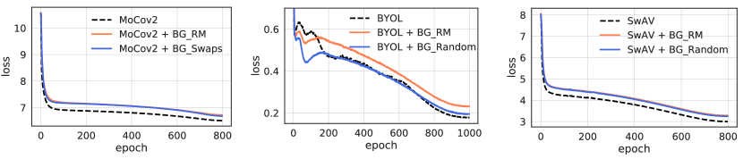
Figure A1: Higher pre-training loss but better generalization. Background augmentations generally lead to a higher final pre-training loss as they make the objective function more “difficult”, but can lead to better generalization.

A.2 Training DeepUSPS²

We trained a DRN-D-105 (Yu et al., 2017) network via BYOL for 500 epochs to an accuracy of 73.9% with the following settings: base learning rate of $0.3$, weight decay of $1\times 10^{-6}$ and momentum coefficient of $0.99$ for the teacher network. All other settings use the defaults for training BYOL. We then use this network as an initialization to train a saliency detector. Note that previous work instead initialized with a network trained using ImageNet class labels as well as CityScapes (Cordts et al., 2016) segmentation labels. We train this network following the procedure from DeepUSPS, but in phase 1 of training, we use a learning rate of $6\times 10^{-6}$ instead of the default value of $1\times 10^{-6}$.

A.3 Linear Evaluation on ImageNet

Linear evaluation protocol was largely similar to original work. For MoCo-v2 and SwAV, we evaluate with a larger batch size to speed up evaluation. We train the linear classifier for more epochs in the case of MoCo-v2 and BYOL to reduce variability in the results. Note that warmup is not required, but for simplicity we opted to keep the training procedure close to standard supervised training.

MoCo-v2.

The linear classifier was trained for 120 epochs, with a step schedule of 60, 80, 100 and a decay factor of 0.1, with a warmup of 10 epochs, a batch size of 2048 (distributed across 32 GPUs). Parameters in the backbone were frozen to the pre-trained values.

BYOL.

The linear classifier was trained for 140 epochs, with a step schedule of 80, 100, 120 and a decay factor of 0.1. We used a base learning rate of 0.2 and a batch size of 1024 distributed across 16 GPUs. Parameters in the backbone were frozen to the pre-trained values.

SwAV.

The linear classifier was trained for 100 epochs with 5 warmup epochs using a batch size of 2048 (distributed across 32 GPUs) and a cosine schedule. Parameters and buffers in the backbone were frozen to the pre-trained values.

RotNet.

The linear evaluation procedure was largely similar to the original paper (Gidaris et al., 2018). A linear classifier was trained on top of Conv5 layer using SGD with Nesterov momentum over 35 epochs using a batchsize of 256 and a momentum of 0.9 with a learning rate of 0.1, a step schedule of (5, 15, 25) and weight decay of $5\times 10^{-4}$.

General Settings.

Following common protocol, pre-processing during training consists of RandomResizedCrop and RandomHorizontalFlip followed by normalization. The pre-processing on validation images consists of Resize to size 256 along the shorter edge of the image, followed by CenterCrop to size 224$\times$224 and normalization.

A.4 Background Augmentations in the Supervised Setting

By default, training followed the settings specified in Methods (Section 2). Here, we discuss implementation details for a) re-training a classifier without background augmentations and b) finetuning the whole network without background augmentations and c) longer training.

A.4.1 Re-training a linear classifier w/o background augmentations

We trained a linear classifier from scratch on top of the frozen trunk without background augmentations using standard pre-processing and data augmentation. We used SGD with momentum of 0.9 , a batchsize of 4096 with a base learning rate of 0.01 and a cosine schedule over 40 epochs and a weight decay of $1\times 10^{-4}$.

A.4.2 Finetuning w/o background augmentations

We finetuned the network without background augmentations, using standard preprocessing and data augmentation. We used SGD with momentum of 0.9 , a batchsize of 4096 with a base learning rate of 0.0005 and a cosine schedule over 20 epochs and a weight decay of $1\times 10^{-4}$.

A.4.3 Longer Training

Training followed the settings specified in Methods (section 2), with the following changes: following CutMix (Yun et al., 2019), training was for 300 epochs with a step schedule of (75, 150, 225).

A.5 Evaluation in Limited-Labels Setting

For consistency with previous work, we use the same fixed splits as in Chen et al. (2020b) for the 1% and 10% labels settings of ImageNet training data.

A.5.1 Linear Evaluation

For simplicity, we train a linear classifier using the same settings as in the corresponding 100% labels linear evaluation, except that we use the training data from the corresponding split (1% or 10%).

A.5.2 Semi-Supervised Evaluation

MoCo-v2/BYOL: We finetuned the network for 50 epochs with a step schedule (30, 40) with a decay factor of 0.1, with a batch size of 256 and no weight decay. For MoCo-v2, in the 1% (10%) label setting, we used a learning rate of 1.0 (0.3) for the classifier head and a learning rate of $1\times 10^{-4}$ ($1\times 10^{-4}$) for the trunk. For BYOL, in the 1% (10%) label setting, we used a learning rate of 1.0 (0.1) for the classifier head and a learning rate of $1\times 10^{-3}$ ($1\times 10^{-3}$) for the trunk. SwAV: we use the same settings as in the original implementation (Caron et al., 2020).

Figure A2: Examples from ImageNet-Renditions. Image from Hendrycks et al. (2021).

A.6 Robustness Evaluations

Robustness evaluations do not involve any additional training—they use the same network (backbone and linear classifier) used for linear evaluation on ImageNet in the 100% labels setting. Note that it is common for robustness benchmarks to use the pre-trained model from torchvision as the supervised baseline. We additionally report metrics using our re-implementation of the standard, stronger supervised baseline in Goyal et al. (2018). We follow the pre-processing protocols from respective original works; unless otherwise mentioned, this is simply the standard way that ImageNet validation images are pre-processed (Appendix A.3).

ImageNet-9.

ImageNet-9 (Xiao et al., 2021a) (IN-9) consists of data sets with varying amount of foreground-background signal. Variations of IN-9 (excluding the “Original”) involve a distribution shift in foreground-background statistics. We use the data and code from the original work for evaluation.

ImageNet-ReaL.

Beyer et al. (2020) relabel the ImageNet validation images to better represent the semantic content present in the images; we use the Reassessed Labels (ReaL) to evaluate ImageNet-ReaL accuracy. Our supervised (torchvision) baseline has an ImageNet-ReaL accuracy of 82.7% (82.9%).

ImageNet-v2.

ImageNet-v2 (Recht et al., 2019) consists of three test data sets for ImageNet, with 10,000 images each. The three variations are a) MatchedFrequency, b) Threshold0.7 and c) TopImages. Accuracies reported in the main text (Section 5.3) correspond to MatchedFrequency. Accuracies for other variations are reported in Appendix D.2.

ObjectNet.

ObjectNet (Barbu et al., 2019) is a test data set that controls for rotation, background, and viewpoint. It contains 50,000 images with 313 object classes. 113 of ObjectNet’s classes overlap with ImageNet—we evaluate on this subset. Following the original work, after removing the one-pixel red border, images are resized to size 224 along the shorter edge, followed by pre-processing steps of CenterCrop and normalization as in Appendix A.3). Our supervised (torchvision) baseline has an ObjectNet accuracy of 24.4% (24.7%).

ImageNet-A.

ImageNet-A (Hendrycks et al., 2019b) is a data set of “natural” adversarial examples—images obtained by a process of adversarial filtering of natural images. It consists of 7,500 images mis-classified by the torchvision ResNet-50 pre-trained model. Hendrycks et al. (2019b) report that a corresponding model re-trained from scratch has an accuracy of 2.2%; our supervised baseline has an accuracy of 2.4%.

ImageNet-R.

ImageNet-R is a data set curated to measure generalization to various abstract visual renditions (e.g. paintings, embroidery, cartoons etc., see Figure A2 for examples) of ImageNet classes. ImageNet-R involves a shift in texture statistics and contains 30,000 images. Our supervised (torchvision) baseline has an ImageNet-R accuracy of 36.0% (36.1%).

Adversarial Attack.

We used foolbox (Rauber et al., 2020) for $\ell_{\infty}$ FGSM adversarial attack with $\epsilon=8/255$ applied to ImageNet validation images.

ImageNet-C.

ImageNet-C (Hendrycks and Dietterich, 2019) consists of 75 test data sets; 15 types of corruptions from four main categories (noise, blur, weather, digital) are applied to ImageNet validation images to generate the test images. Each corruption type has five levels of severity. We report the average performance on the four main categories of corruptions in Appendix D.4. Pre-processing steps are CenterCrop and normalization as in Appendix A.3.

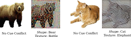
Figure A3: Examples with and without texture-shape cue conflict.

A.7 Shape-Bias Evaluation

The shape-bias (Geirhos et al., 2019) of a model is computed using texture-shape cue conflict stimuli (the shape and texture cues in the image correspond to different ImageNet classes, e.g. see Figure A3) as the fraction of classification decisions that correspond to shape information; this computation only considers the subset of “correctly” classified images—either the shape or texture category are correctly classified. Images are pre-processed as in Appendix A.3.

A.8 Linear Evaluation on CIFAR-10, 100

All methods were evaluated using the same protocol for fair comparison. A linear classifier was trained with SGD with momentum 0.9 for 100 epochs with a base learning rate of 0.08, a batch size of 32 and a cosine learning rate schedule.

A.9 Linear Evaluation on Places-205

All methods were evaluated using the same protocol for fair comparison. A linear classifier was trained with SGD with momentum 0.9 for 28 epochs with a base learning rate of 1.0, a batch size of 256 and a step schedule of 7, 14, 21 and a decay factor of 0.1. Weight decay was set to 0.0001.

A.10 Object Detection and Instance Segmentation

We follow standard protocol across all SSL methods: a) VOC detection: We finetuned a Faster R-CNN (Ren et al., 2015) in VOC 2007 + 2012 trainval for 24k iterations and evaluated in VOC 2007 test, b) COCO detection and COCO instance segmentation: We fine-tuned a Mask R-CNN (He et al., 2017) (2× schedule) in COCO 2017 train, evaluated in COCO 2017 val. All Faster/Mask R-CNN models are with the C4-backbone. We use Detectron2 (Wu et al., 2019) for all experiments.

VOC: For MoCo-v2 and SwAV, we followed the settings from their corresponding original papers. In the case of BYOL, we followed the settings of MoCo-v2 with one deviation: we used a base learning rate of $0.08$. COCO: we used the default settings of MoCo-v2 for all methods.

B Characterizing the Impact of Mask Quality

While the results in Section 4.7 show that there may be diminishing gains to using higher quality masks than those provided by DeepUSPS², it does not give us a clear picture of the impact of mask quality. For example, one may wonder,

• How does performance vary as a function of mask quality?

• Which SSL methods and background augmentations are more robust to mask quality?

To answer these questions, and in an attempt to gain further insight into the mechanism by which background augmentations improve representations, we systematically perturb the quality of the foreground masks. In these experiments, we use U²Net to generate the initial foreground masks (that we then perturb) to minimize the possibility of starting with a poor mask and maintain greater control over the quality of a perturbed mask.

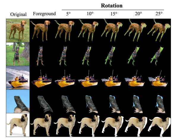
Figure A4: Mask Distortion: Rotation. Examples of varying distortion strength.

We perturb the masks in numerous ways across a range of distortion strengths/levels. The distortions we consider are: a) rotation (see Figure A4 for examples), b) shearing (Figure A5), c) translation (Figure A6), d) horizontal flips and e) using bounding-box masks instead of the original mask (Figure A7). We expect mask translation and using bounding-box masks to be particularly challenging.

	MoCo-v2			BYOL		SwAV
Max Rotation	baseline	BG_RM	BG_Swaps	baseline	BG_RM	baseline	BG_RM
0∘	67.7	69.3 (+1.6)	69.7 (+2.0)	72.7	73.5 (+0.8)	72.2	73.7 (+1.5)
5∘	-	69.3 (+1.6)	69.3 (+1.6)	-	73.1 (+0.4)	-	73.7 (+1.5)
10∘	-	69.0 (+1.3)	69.3 (+1.6)	-	73.3 (+0.6)	-	73.6 (+1.4)
15∘	-	68.7 (+1.0)	69.4 (+1.7)	-	73.3 (+0.6)	-	73.3 (+1.1)
20∘	-	68.7 (+1.0)	69.1 (+1.4)	-	73.1 (+0.4)	-	73.5 (+1.3)
25∘	-	68.4 (+0.7)	69.0 (+1.3)	-	73.1 (+0.4)	-	73.5 (+1.3)

Table A1: Mask Distortion: Rotation. Background augmentations are robust to substantial mask noise induced via rotations of the foreground mask. Of note, BG_Swaps maintains a large performance benefit even for strong distortions. We highlight the $\Delta$ relative to the baselines with no background augmentations.

We characterize the dependence on mask quality for BG_RM across all the view-invariant SSL methods in our test bed; in the case of MoCo-v2, we additionally include BG_Swaps. We apply the respective distortion to each mask, every time it is used in a background augmentation. All experiments are in the respective medium duration settings; we report ImageNet accuracy. We make the following observations:

Low quality masks can still be beneficial.

Overall, we find that there is substantial robustness to mask quality. In many instances, only a little of the foreground remains in view, yet background augmentations maintain improved performance over the baseline. We find that mask translation and using bounding-box masks are particularly challenging distortions as expected—surprisingly, some performance benefits persist (but quickly disappear with higher distortion strength).

SwAV and BG_Swaps are quite robust to mask quality.

We find that BG_Swaps is far more robust to mask quality compared to BG_RM across all variants and degrees of distortions, showcasing the robustness of this augmentation method. For example, across rotation, shearing, translation and flip distortions, the improvement due to BG_Swaps is $\sim$2-3$\times$ the improvement due to BG_RM in the respective strongest distortion levels; further, when the foreground mask is replaced with a bounding-box mask, the benefit due to BG_RM disappears, while BG_Swaps retains a significant performance benefit.

Among the SSL methods in our test bed, SwAV appears to be most robust to mask quality, managing to maintain significant performance benefits even with strong mask distortion. We speculate that this may be linked to use of multi-crop augmentation wherein local crops are expected to be predictive of global crops. When background augmentations are applied using distorted masks, only a small part of the foreground may be featured in a view—much like a local crop in multi-crop augmentation.

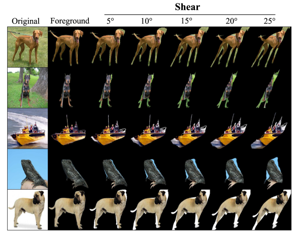
Figure A5: Mask Distortion: Shearing. Examples of varying distortion strength.

	MoCo-v2			BYOL		SwAV
Max Shear	baseline	BG_RM	BG_Swaps	baseline	BG_RM	baseline	BG_RM
0∘	67.7	69.3 (+1.6)	69.7 (+2.0)	72.7	73.5 (+0.8)	72.2	73.7 (+1.5)
5∘	-	69.2 (+1.5)	69.3 (+1.6)	-	73.2 (+0.5)	-	73.5 (+1.3)
10∘	-	68.8 (+1.1)	69.2 (+1.5)	-	73.5 (+0.8)	-	73.6 (+1.4)
15∘	-	68.6 (+0.9)	69.4 (+1.7)	-	73.0 (+0.3)	-	73.5 (+1.3)
20∘	-	68.3 (+0.6)	69.0 (+1.3)	-	73.2 (+0.5)	-	73.4 (+1.2)
25∘	-	68.1 (+0.4)	68.9 (+1.2)	-	72.9 (+0.2)	-	73.5 (+1.3)

Table A2: Mask Distortion: Shearing. Background augmentations are robust to substantial mask noise induced via shearing of the foreground mask. Of note, BG_Swaps maintains a large performance benefit even for strong distortions. We highlight the $\Delta$ relative to the baselines with no background augmentations.

B.1 Implementation Details.

Every mask was perturbed prior to background augmentations in every epoch. Rotation. Each mask was subject to random rotation sampled between $(-\text{max rot.},+\text{max rot.})$. Shearing. Each mask was subject to shearing independently along $x$ and $y$ coordinates with a value uniformly sampled from $(-\text{max shear},+\text{max shear})$. Translation. Each mask was subject to translation independently along the width and height with values uniformly sampled from $(-\text{max trans.},+\text{max trans.})\times\text{max FG width}$ and $(-\text{max trans.},+\text{max trans.})\times\text{max FG height}$ respectively. Horizontal Flip. Each mask was horizontally flipped with a probability 0.5 (on each use of the mask). Bounding-Box Masks. Binary foreground masks were used to generate rectangular bounding-box masks of size max FG width $\times$ max FG height.

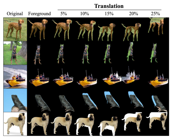
Figure A6: Mask Distortion: Translation. Examples of varying distortion strength.

	MoCo-v2			BYOL		SwAV
Max Translation	baseline	BG_RM	BG_Swaps	baseline	BG_RM	baseline	BG_RM
0%	67.7	69.3 (+1.6)	69.7 (+2.0)	72.7	73.5 (+0.8)	72.2	73.7 (+1.5)
5%	-	68.9 (+1.2)	69.5 (+1.8)	-	73.3 (+0.6)	-	73.3 (+1.1)
10%	-	68.7 (+1.0)	69.2 (+1.5)	-	73.3 (+0.6)	-	73.5 (+1.3)
15%	-	68.2 (+0.5)	68.7 (+1.0)	-	73.1 (+0.4)	-	73.2 (+1.0)
20%	-	68.0 (+0.3)	68.7 (+1.0)	-	73.1 (+0.4)	-	73.3 (+1.1)
25%	-	67.9 (+0.2)	68.3 (+0.6)	-	72.9 (+0.2)	-	73.0 (+0.8)

Table A3: Mask Distortion: Translation. Background augmentations are robust to substantial mask noise induced via translation of the foreground mask. Of note, BG_Swaps maintains a large performance benefit even for strong distortions. We highlight the $\Delta$ relative to the baselines with no background augmentations.

	MoCo-v2			BYOL		SwAV
Random Horizontal Flip	baseline	BG_RM	BG_Swaps	baseline	BG_RM	baseline	BG_RM
✗	67.7	69.3 (+1.6)	69.7 (+2.0)	72.7	73.5 (+0.8)	72.2	73.7 (+1.5)
✓	-	68.7 (+1.0)	69.4 (+1.7)	-	73.3 (+0.6)	-	73.5 (+1.3)

Table A4: Mask Distortion: Horizontal Flip. Background augmentations are robust to substantial mask noise induced via horizontal flip of the foreground mask. Of note, BG_Swaps maintains a large performance benefit even for strong distortions. We highlight the $\Delta$ relative to the baselines with no background augmentations.

	MoCo-v2			BYOL		SwAV
	baseline	BG_RM	BG_Swaps	baseline	BG_RM	baseline	BG_RM
Saliency mask	67.7	69.3 (+1.6)	69.7 (+2.0)	72.7	73.5 (+0.8)	72.2	73.7 (+1.5)
Bounding-box mask	-	67.8 (+0.1)	68.7 (+1.0)	-	73.0 (+0.3)	-	73.0 (+0.8)

Table A5: Mask Distortion: Bounding-Box Mask. BG_Swaps is robust even to replacing the mask with a bounding-box mask. Notably, SwAV also manages to retain some performance benefit even in this extreme setting.

C Ablations

Here, we report additional ablations of design choices and hyperparameter settings. We also provide additional information regarding ablations in the main text. To control for mask quality, we use U²Net to generate foreground masks unless otherwise indicated. We report ImageNet accuracy.

C.1 Augmentation Strength

We ablate the strength of background augmentations and find that $p\in[0.1,0.3]$ is generally a good setting. For MoCo-v2, as previously discussed, though BG_RM is more (Out-of-Distribution) OOD than BG_Random, the presence of negatives in the queue $Q$ with (gray) backgrounds similar to $q$ offsets this and results in better performance than BG_Random across all augmentation strengths, see Table A6.

Baseline (67.7)	$p=0.1$	$p=0.2$	$p=0.3$	$p=0.4$	$p=0.5$
BG_RM	69.3	69.3	69.3	68.8	68.4
BG_Random	69.1	69.2	68.6	67.8	66.8

Table A6: MoCo-v2: Ablating the strength of background augmentations BG_RM and BG_Random.

Baseline (67.7)	$p_{\text{neg}}=0.1$	$p_{\text{neg}}=0.2$	$p_{\text{neg}}=0.3$	$p_{\text{neg}}=0.4$	$p_{\text{neg}}=0.5$
$p_{\text{pos}}=0.1$	69.2	69.6	69.7	69.6	69.7
$p_{\text{pos}}=0.2$	69.5	69.7	69.5	69.5	69.7
$p_{\text{pos}}=0.3$	68.9	69.3	69.3	69.0	69.3

Table A7: MoCo-v2: Ablating the strength of background augmentation BG_Swaps.

As discussed in Section 4.4, BG_Swaps overcomes the OOD issue of BG_RM by using cached random natural backgrounds in $q$ and $k^{+}$ with a probability $p_{\text{pos}}$ and additionally includes an extra negative whose background matches $q$ with a probability $p_{\text{neg}}$. As can be seen in Table A7, this results in substantially improved performance at each level of $p_{\text{pos}}$ over the corresponding level of BG_Random. Performance is more sensitive to $p_{\text{pos}}$ than to $p_{\text{neg}}$ and $p_{\text{pos}}$$\simeq$$p_{\text{neg}}$ is generally a reasonable setting. Performance as a function of augmentation strength for BYOL and SwAV are shown in Tables A8 and A9. In all of the above ablations, $\text{FG}_{\text{min}}=0$, i.e. no constraints were imposed on RRC regarding the foreground.

C.2 Do Multiple Matched Negatives Help?

We investigated using multiple background matched negatives in BG_Swaps but found that it did not confer further improvements in performance. We obtained 68.9% ImageNet accuracy using 5 matched negatives vs. 68.8% using 1 matched negative, suggesting that there may be little benefit to increasing the number of background matched negatives. In these experiments, there were no background augmentations in $q$, only in $k^{+}$ and $k^{-}$; $p_{\text{pos}}=p_{\text{neg}}=0.2$ and background augmented negatives matched the background of $k^{+}$.

C.3 Is it a Better Teaching Signal for Background Augmentations in the Positive and Negative to be Independent or Coupled?

To answer this question, we contrasted independent background augmentations in BG_Swaps in $k^{+}$ and $k^{-}$ with coupled background augmentations in $k^{+}$ and $k^{-}$. We observed identical performance of 68.8% in each case. Other experiment settings as in C.2.

C.4 Is it Better for a Negative’s Background to Match $q$ or $k^{+}$?

We observed similar results in both cases a) background matches $q$ (68.9%) and b) background matches $k^{+}$ (68.8%). Other experiment settings as in C.2.

C.5 Order of Augmentations

As noted in Section 2.2, by default, we apply background augmentations after all other augmentations in the respective pipeline. Here, we show that background augmentation before all other augmentations produces similar results. We apply BG_Random in SwAV with $p=0.1$ and find corresponding accuracies of 73.4% (before) vs. 73.2% (after). Similarly, applying BG_RM with $p=0.1$ in MoCo-v2, we find corresponding accuracies of 69.6% (before) vs. 69.3% (after).

Baseline (72.7)	$p=0.05$	$p=0.1$	$p=0.15$	$p=0.2$	$p=0.25$
BG_RM	73.7	73.6	73.8	73.5	73.1
BG_Random	73.7	73.9	73.5	73.4	72.7

Table A8: BYOL: Ablating the strength of background augmentations BG_RM and BG_Random.

Baseline (72.2)	$p=0.05$	$p=0.1$	$p=0.15$	$p=0.2$	$p=0.25$	$p=0.3$
BG_RM	73.1	73.5	73.5	73.5	73.6	73.7
BG_Random	73.0	73.2	73.2	73.7	70.9	67.2

Table A9: SwAV: Ablating the strength of background augmentations BG_RM and BG_Random.

C.6 Influence of Random Crop

RandomResizedCrop (RRC) is a critical part of current SSL pipelines. Indeed, replacing RRC with CenterCrop results in very poor accuracy, 26.8% for MoCo-v2, see Table A10 (b). Concretely, instead of RRC, we first Resize to size 256 along the shorter edge of the image, followed by a CenterCrop to size 224$\times$224. Interestingly, using BG_Swaps with CenterCrop can substantially improve performance (c) over CenterCrop alone, though the performance is still far reduced from using RRC. This raises an intriguing possibility: perhaps one role of RRC is to bootstrap learning background invariance. Future work could potentially investigate this hypothesis.

One effect of RRC is that only a little of the foreground may be present in a view. We investigate the effect of including a lower bound on the amount of foreground included in a view. Concretely, we generate the parameters for RRC imposing one additional constraint: that $\text{FG}_{\text{min}}$ fraction of the foreground be present in the resulting crop. The foreground area is obtained from the corresponding binary foreground mask. Thus, no constraint corresponds to $\text{FG}_{\text{min}}=0$. Too large a value of $\text{FG}_{\text{min}}$ can be expected to hurt performance, since it overly constrains RRC which is useful for inducing desirable invariances (e.g. occlusion or scale invariance). Crop parameters are sampled in the standard way, defaulting to a CenterCrop if the sampled RRC parameters are rejected 10 times.

We find that this strategy of imposing a foreground constraint can help when the setting of background augmentation strength is lower than optimal, but it adds little benefit (if any) on top of optimal settings, see Table A11. As another example, consider SwAV, where BG_RM (BG_Random) results in an accuracy of 73.6% (73.7%) with $\text{FG}_{\text{min}}=0$, see Table A9. We find no benefit when we impose a constraint of $\text{FG}_{\text{min}}=0.15$, with corresponding accuracies for BG_RM (BG_Random) of 73.7% (73.5%), see Table 5.

	RRC	CenterCrop	BG_Swaps	ImageNet acc.
baseline	✓			67.7
(a)	✓		✓	69.2
(b)		✓		26.8
(c)		✓	✓	49.6

Table A10: Impact of RandomResizedCrop. RRC is critical for good performance in current SSL pipelines. In MoCo-v2, replacing RRC with CenterCrop significantly hurts performance, but application of BG_Swaps somewhat helps compensate. Aug. Strength of BG_Swaps: $p_{\text{pos}}=p_{\text{neg}}=0.1$.

Baseline (67.7)	$\text{FG}_{\text{min}}=0$	$\text{FG}_{\text{min}}=0.1$	$\text{FG}_{\text{min}}=0.2$
$p_{\text{pos}}=p_{\text{neg}}=0.1$	69.2	69.7	69.4
$p_{\text{pos}}=p_{\text{neg}}=0.2$	69.7	69.8	69.5

Table A11: Impact of including more foreground in views. Constraining RRC to include more of the foreground in MoCo-v2, we see that it can be beneficial when the setting of background augmentation (BG_Swaps) strength is lower than optimal, but confers little (if any) benefit on top of the optimal setting of background augmentation strength.

C.7 Sensitivity of SwAV

Ease of Optimization.

We observe that SwAV is more sensitive to high amount of background augmentations when using using BG_Random, with performance degrading less gracefully than BYOL or MoCo-v2 when the strength of background augmentation is high. We linked this behavior to the difficulty of the optimization task of learning invariance to random natural backgrounds in conjunction with SwAV’s objective function. As discussed in Section 4.6, this can be alleviated by increasing the capacity of the projection MLP or by warming up the background augmentations, resulting in stable performance even at very strong augmentation strength, see Figure 4. We linearly warmed up background augmentation strength over 10 epochs.

Crop Scale Ablation.

Parametrizing the scale setting for local and global crops as $(0.05,s)$ and $(s,1)$, the default setting uses $s=0.14$. As discussed in Section 4.6, we find that increasing $s$ can help improve performance when used in conjunction with background augmentations. For BG_RM (BG_Random), we used $s=0.26$ ($s=0.2$). We used a 5 epoch linear warmup of background augmentation strength. We found that increasing $s$ to 0.2 for the SwAV baseline, i.e. without background augmentations, results in failure—the loss at the end of pre-training is at chance. The projection MLP capacity was set to 4096/256 in all cases.

Temperature Sensitivity.

We also note that we observed high sensitivity to the temperature setting in SwAV, in contrast with MoCo-v2. Future work could investigate the source of this sensitivity, potentially further improving performance.

General Settings.

All ablations discussed here (Appendix C.7, Section 4.6) use defaults for remaining settings except the experiments with the default projection MLP capacity (2048/128)—these numbers are from the ablation of augmentation strength in Appendix C.1.

C.8 Does BN Adaptation Help?

Due to strong augmentation during SSL pre-training, the statistics of images during pre-training may be different from those in downstream application, e.g. linear evaluation on ImageNet. Intuitively, one might expect that adapting BN statistics might result in improved performance. Indeed, in the supervised setting, it has been shown (Schneider et al., 2020; Nado et al., 2020) that adapting the batch normalization (BN) statistics under distribution shift can result in improved performance. Here, we consider linear evaluation on ImageNet with and without adaptation of BN statistics in the backbone. Specifically, for adaptation (no adaptation), we use train (eval) mode for BN layers while training the linear classifier and eval (eval) model during evaluation. Intriguingly, we find that adaptation does not necessarily result in improved performance.

Note that no supervised information is used for BN adaptation. All parameters in the backbone remain frozen to their pre-trained values. All models received full pre-training. Background augmentations used DeepUSPS².

Method	ImageNet acc.
	w/o adapt.	w/ adapt.
MoCo-v2 (repro.)	71.0	71.0
MoCo-v2 + BG_RM	71.9	71.9
MoCo-v2 + BG_Swaps	72.1	72.2
BYOL (repro.)	74.1	73.8
BYOL + BG_RM	75.1	74.6
BYOL + BG_Random	75.2	74.8
SwAV (repro.)	74.9	74.7
SwAV + BG_RM	76.1	75.1
SwAV + BG_Random	76.1	75.1

Table A12: Impact of Adapting BN Statistics. Adaptation does not necessarily result in improved performance.

C.9 Additional Information for Ablations in Main Text

Ablations in Tables 3, 4 follow the settings in Appendix C.1 and use $\text{FG}_{\text{min}}=0$.

D Additional Results

Here we report additional results, including downstream evaluations of corresponding models which used U²Net for generating foreground masks—evaluations of these models are consistent with evaluations of corresponding DeepUSPS² models; we therefore skip detailed discussions of these specific results.

D.1 ImageNet-9

We expand on results in Table 10 in Table A14 to include SEM, which was excluded in the main text to avoid clutter. These results correspond to medium duration pre-trained models. We report corresponding results for the full duration pre-trained models in Table A15. Corresponding tables for U²Net are Tables A16 and A17; for convenience, we report also report corresponding BG-Gap in Table A18.

Method		1% Labels		10% Labels
		Top-1	Top-5	Top-1	Top-5
Supervised		25.4	48.4	56.4	80.4
Linear	MoCo-v2 (repro.)	52.0	77.7	63.9	85.8
	MoCo-v2 + BG_RM	54.4 (+2.4)	78.7	65.2 (+1.3)	86.3
	MoCo-v2 + BG_Swaps	56.4 (+4.4)	79.8	65.8 (+1.9)	86.5
	BYOL (repro.)	57.5	80.8	68.6	88.6
	BYOL + BG_RM	60.8 (+3.3)	82.9	70.2 (+1.6)	89.3
	BYOL + BG_Random	61.0 (+3.5)	83.5	70.6 (+2.0)	89.6
	SwAV (repro.)	52.8	78.4	68.3	88.7
	SwAV + BG_RM	57.6 (+4.8)	81.8	70.3 (+2.0)	89.8
	SwAV + BG_Random	56.4 (+3.6)	80.8	70.3 (+2.0)	89.8
Finetune	MoCo-v2 (repro.)	54.1	81.3	67.6	89.4
	MoCo-v2 + BG_RM	55.3 (+1.2)	81.4	68.0 (+0.4)	89.3
	MoCo-v2 + BG_Swaps	57.7 (+3.6)	82.7	68.8 (+1.2)	89.6
	BYOL (repro.)	57.3	80.5	70.6	90.0
	BYOL + BG_RM	60.5 (+3.2)	82.6	71.7 (+1.1)	90.6
	BYOL + BG_Random	60.7 (+3.4)	83.1	71.9 (+1.3)	90.8
	SwAV (repro.)	54.0	78.5	70.1	89.9
	SwAV + BG_RM	54.7 (+0.7)	78.9	70.7 (+0.6)	90.2
	SwAV + BG_Random	55.7 (+1.7)	79.3	70.8 (+0.7)	90.2

Table A13: Limited-Labels Setting. Background augmentations improve performance in the limited-labels setting. Linear evaluation using 100% of ImageNet labels though a standard benchmark, is a somewhat unrealistic setting. Evaluation in the more practical setting of limited-labels reveals even larger improvement in performance. We highlight performance gains due to background augmentations. Similar to Table 6, but U²Net was used for foreground extraction. Best (second best) results are in bold (underlined).

Data Set	Supervised	MoCo-v2			BYOL			SwAV
		baseline	BG_RM	BG_Swaps	baseline	BG_RM	BG_Random	baseline	BG_RM	BG_Random
Original	95.6	92.7	93.8	94.2	94.9	95.6	96.0	94.1	95.0	94.9
Only-BG-B $\downarrow$	11.4	6.1	6.1	3.6	5.4	4.9	6.0	10.9	8.8	8.3
Only-BG-T $\downarrow$	16.3	14.8	12.9	9.3	12.7	11.8	11.5	15.8	16.7	17.6
No-FG	45.9	37.8	42.3	39.6	43.9	45.9	46.2	41.3	44.2	45.2
Only-FG $\uparrow$	86.8	74.4	81.9$\pm$0.1 (+7.5)	86.1$\pm$0.4 (+11.7)	83.5	88.8$\pm$0.1 (+5.3)	87.7$\pm$0.6 (+4.2)	79.4	85.3$\pm$0.1 (+5.9)	84.3$\pm$0.2 (+4.9)
Mixed-Same $\uparrow$	86.2	81.8	84.0$\pm$0.1 (+2.2)	87.9$\pm$0.3 (+6.1)	86.2	88.6$\pm$0.2 (+2.4)	90.1$\pm$0.1 (+3.9)	82.2	86.1$\pm$0.3 (+3.9)	86.3$\pm$0.2 (+4.1)
Mixed-Rand $\uparrow$	78.9	70.7	76.3$\pm$0.2 (+5.6)	84.1$\pm$0.3 (+13.4)	79.6	83.2$\pm$0.1 (+3.6)	85.5$\pm$0.3 (+5.9)	71.3	77.1$\pm$0.3 (+5.8)	77.0$\pm$0.3 (+5.7)
Mixed-Next $\uparrow$	77.2	67.0	73.0$\pm$0.1 (+6.0)	82.2$\pm$0.4 (+15.2)	77.6	80.7$\pm$0.1 (+3.1)	84.0$\pm$0.1 (+6.4)	69.0	74.3$\pm$0.2 (+5.3)	74.4$\pm$0.2 (+5.4)

Table A14: Robustness: Foreground-Background Shifts. Background augmentations result in large performance gains on ImageNet-9 (IN-9) across all SSL methods, with BG_Swaps generally exhibiting similar or better performance than BG_RM. We highlight the performance benefit on the variants of IN-9 especially relevant to our work. All pre-training durations correspond to respective medium settings. Note that IN-9 uses only 9 classes, so chance is $\sim$11.1%. This table is an expanded version of Table 10, to include SEM which were excluded in the main text to avoid clutter.

Data Set	Supervised	MoCo-v2			BYOL			SwAV
		baseline	BG_RM	BG_Swaps	baseline	BG_RM	BG_Random	baseline	BG_RM	BG_Random
Original	95.6	94.7	94.9	95.3	95.2	95.8	95.7	94.6	95.4	95.1
Only-BG-B $\downarrow$	11.4	7.9	6.3	5.1	7.1	5.8	6.0	11.4	10.5	10.9
Only-BG-T $\downarrow$	16.3	14.7	13.9	11.1	16.5	13.0	14.1	19.2	18.3	18.0
No-FG	45.9	42.3	43.5	42.6	42.7	46.5	47.5	46.0	47.4	43.5
Only-FG $\uparrow$	86.8	79.7	85.2 (+5.5)	86.9 (+7.2)	81.4	88.5 (+7.1)	87.3 (+5.9)	81.9	84.1 (+2.2)	83.2 (+1.3)
Mixed-Same $\uparrow$	86.2	84.9	85.8 (+0.9)	89.7 (+4.8)	86.7	89.2 (+2.5)	90.2 (+3.5)	84.3	86.0 (+1.7)	85.5 (+1.2)
Mixed-Rand $\uparrow$	78.9	74.9	79.0 (+4.1)	85.3 (+10.4)	77.6	83.9 (+6.3)	85.8 (+8.2)	72.9	76.7 (+3.8)	76.5 (+3.9)
Mixed-Next $\uparrow$	77.2	72.9	76.0 (+3.1)	82.7 (+9.8)	75.7	82.0 (+6.3)	84.1 (+8.4)	70.2	74.5 (+4.3)	73.1 (+2.9)

Table A15: Robustness: Foreground-Background Shifts. Background augmentations result in large performance gains on ImageNet-9 (IN-9) across all SSL methods, with BG_Swaps generally exhibiting similar or better performance than BG_RM. We highlight the performance benefit on the variants of IN-9 especially relevant to our work. All pre-training durations correspond to respective full settings. Note that IN-9 uses only 9 classes, so chance is $\sim$11.1%.

Data Set	Supervised	MoCo-v2			BYOL			SwAV
		baseline	BG_RM	BG_Swaps	baseline	BG_RM	BG_Random	baseline	BG_RM	BG_Random
Original	95.6	92.7	94.1	94.4	94.9	95.8	95.9	94.1	94.8	94.7
Only-BG-B $\downarrow$	11.4	6.1	7.2	4.2	5.4	4.9	5.8	10.9	8.5	8.7
Only-BG-T $\downarrow$	16.3	14.8	13.8	10.7	12.7	12.0	12.2	15.8	16.6	17.2
No-FG	45.9	37.8	43.5	41.7	43.9	46.5	46.2	41.3	46.1	45.3
Only-FG $\uparrow$	86.8	74.4	83.6$\pm$0.3 (+9.2)	85.4$\pm$0.1 (+11)	83.5	89.3$\pm$0.5 (+5.8)	87.6$\pm$0.4 (+4.1)	79.4	85.4$\pm$0.2 (+6.0)	85.3$\pm$0.2 (+5.9)
Mixed-Same $\uparrow$	86.2	81.8	85.6$\pm$0.2 (+3.8)	88.2$\pm$0.2 (+6.4)	86.2	89.0$\pm$0.3 (+2.8)	90.4$\pm$0.3 (+4.2)	82.2	86.0$\pm$0.4 (+3.8)	86.1$\pm$0.1 (+3.9)
Mixed-Rand $\uparrow$	78.9	70.7	78.2$\pm$0.2 (+7.5)	83.6$\pm$0.2 (+12.9)	79.6	83.8$\pm$0.1 (+4.2)	85.3$\pm$0.2 (+5.7)	71.3	76.7$\pm$0.1 (+5.4)	76.8$\pm$0.3 (+5.5)
Mixed-Next $\uparrow$	77.2	67.0	75.2$\pm$0.1 (+8.2)	81.2$\pm$0.2 (+14.2)	77.6	81.7$\pm$0.1 (+4.1)	83.5$\pm$0.3 (+5.9)	69.0	73.8$\pm$0.4 (+4.8)	74.1$\pm$0.2 (+5.1)

Table A16: Robustness: Foreground-Background Shifts. Background augmentations result in large performance gains on ImageNet-9 (IN-9) across all SSL methods, with BG_Swaps generally exhibiting similar or better performance than BG_RM. We highlight the performance benefit on the variants of IN-9 especially relevant to our work. All pre-training durations correspond to respective medium settings. Note that IN-9 uses only 9 classes, so chance is $\sim$11.1%. Similar to Table A14, but U²Net was used for FG extraction.

Data Set	Supervised	MoCo-v2			BYOL			SwAV
		baseline	BG_RM	BG_Swaps	baseline	BG_RM	BG_Random	baseline	BG_RM	BG_Random
Original	95.6	94.7	94.8	95.2	95.2	96.1	96.1	94.6	95.3	95.4
Only-BG-B $\downarrow$	11.4	7.9	8.1	3.4	7.1	4.8	6.2	11.4	10.3	13.6
Only-BG-T $\downarrow$	16.3	14.7	14.2	11.4	16.5	13.8	12.9	19.2	18.2	18.6
No-FG	45.9	42.3	45.5	43.0	42.7	47.9	48.1	46.0	46.8	44.9
Only-FG $\uparrow$	86.8	79.7	87.1 (+7.4)	87.5 (+7.8)	81.4	89.1 (+7.7)	88.3 (+6.9)	81.9	86.8 (+4.9)	83.8 (+1.9)
Mixed-Same $\uparrow$	86.2	84.9	87.1 (+2.2)	89.6 (+4.7)	86.7	89.5 (+2.8)	90.2 (+3.5)	84.3	87.0 (+2.7)	86.9 (+2.6)
Mixed-Rand $\uparrow$	78.9	74.9	80.7 (+5.8)	85.2 (+10.3)	77.6	84.2 (+6.6)	85.2 (+7.6)	72.9	77.1 (+4.2)	76.6 (+3.7)
Mixed-Next $\uparrow$	77.2	72.9	78.1 (+5.2)	83.2 (+10.3)	75.7	81.7 (+6.0)	83.8 (+8.1)	70.2	75.6 (+5.4)	74.3 (+4.1)

Table A17: Robustness: Foreground-Background Shifts. Background augmentations result in large performance gains on ImageNet-9 (IN-9) across all SSL methods, with BG_Swaps generally exhibiting similar or better performance than BG_RM. We highlight the performance benefit on the variants of IN-9 especially relevant to our work. All pre-training durations correspond to respective full settings. Note that IN-9 uses only 9 classes, so chance is $\sim$11.1%. Similar to Table A15, but U²Net was used for FG extraction.

Pre-Train Duration	MoCo-v2			BYOL			SwAV
	baseline	BG_RM	BG_Swaps	baseline	BG_RM	BG_Random	baseline	BG_RM	BG_Random
Med.	11.1	7.4 (-3.7)	4.6 (-6.5)	6.6	5.2 (-1.4)	5.1 (-1.5)	10.9	9.3 (-1.6)	9.3 (-1.6)
Full	10.0	6.4 (-3.6)	4.4 (-5.6)	9.1	5.3 (-3.8)	5.0 (-4.1)	11.4	9.9 (-1.5)	10.3 (-1.1)

Table A18: BG-Gap: Background augmentations decrease BG-Gap of SSL Methods. Similar to Table 11, but U²Net was used for FG extraction.

D.2 ImageNet-v2

Here, we report evaluation on all variants of ImageNet-v2: MatchedFrequency (MF), Threshold0.7 (T0.7) and TopImages (TI). Background augmentations result in large performance gains across all variants. Corresponding results for U²Net are shown in Table A20.

Method	ImageNet-v2 acc.
	MF	T0.7	TI
Supervised	63.8	72.6	77.7
Pre-Train Duration: Medium
MoCo-v2 (repro.)	54.7	63.6	69.6
MoCo-v2 + BG_RM	56.7$\pm$0.1 (+2.0)	65.7$\pm$0.1 (+2.1)	71.5$\pm$0.1 (+1.9)
MoCo-v2 + BG_Swaps	57.2$\pm$0.1 (+2.5)	66.3$\pm$0.1 (+2.7)	72.0$\pm$0.2 (+2.4)
BYOL (repro.)	60.7	70.2	75.6
BYOL + BG_RM	61.7$\pm$0.2 (+1.0)	71.0$\pm$0.2 (+0.8)	76.3$\pm$0.2 (+0.7)
BYOL + BG_Random	62.1$\pm$0.1 (+1.4)	71.5$\pm$0.0 (+1.3)	76.7$\pm$0.1 (+1.1)
SwAV (repro.)	59.3	68.5	73.9
SwAV + BG_RM	61.2$\pm$0.3 (+1.9)	70.3$\pm$0.1 (+1.8)	75.6$\pm$0.1 (+1.7)
SwAV + BG_Random	60.7$\pm$0.0 (+1.4)	70.0$\pm$0.2 (+1.5)	75.3$\pm$0.1 (+1.4)
Pre-Train Duration: Full
MoCo-v2 (repro.)	58.9	67.4	73.1
MoCo-v2 + BG_RM	59.6 (+0.7)	68.7 (+1.3)	74.2 (+1.1)
MoCo-v2 + BG_Swaps	60.3 (+1.4)	68.8 (+1.4)	74.9 (+1.8)
BYOL (repro.)	61.9	71.2	76.2
BYOL + BG_RM	63.4 (+1.5)	72.4 (+1.2)	77.7 (+1.5)
BYOL + BG_Random	62.8 (+0.9)	72.4 (+1.2)	77.2 (+1.0)
SwAV (repro.)	61.7	70.8	76.4
SwAV + BG_RM	63.8 (+2.1)	72.8 (+2.0)	77.9 (+1.5)
SwAV + BG_Random	63.4 (+1.7)	72.3 (+1.5)	77.9 (+1.5)

Table A19: Robustness: Natural Distribution Shift. Expanded version of Table 12. Background augmentations improve performance on all variants of ImageNet-v2. Notably, background augmentations enable SwAV to perform on par with the standard supervised baseline. Best results are in bold. Notation: MF=MatchedFrequency, T0.7=Threshold0.7, TI=TopImages. Results in Table 12 correspond to MF and are included here for completeness.

Method	ImageNet-v2 acc.
	MF	T0.7	TI
Supervised	63.8	72.6	77.7
Pre-Train Duration: Medium
MoCo-v2 (repro.)	54.7	63.6	69.6
MoCo-v2 + BG_RM	57.0$\pm$0.1 (+2.3)	66.2$\pm$0.2 (+2.6)	71.8$\pm$0.1 (+2.2)
MoCo-v2 + BG_Swaps	57.6$\pm$0.0 (+2.9)	66.5$\pm$0.2 (+2.9)	72.3$\pm$0.1 (+2.7)
BYOL (repro.)	60.7	70.2	75.6
BYOL + BG_RM	62.2$\pm$0.2 (+1.5)	71.3$\pm$0.1 (+1.1)	76.5$\pm$0.1 (+0.9)
BYOL + BG_Random	62.2$\pm$0.4 (+1.5)	71.5$\pm$0.1 (+1.3)	76.6$\pm$0.2 (+1.0)
SwAV (repro.)	59.3	68.5	73.9
SwAV + BG_RM	61.2$\pm$0.1 (+1.9)	70.2$\pm$0.2 (+1.7)	75.4$\pm$0.1 (+1.5)
SwAV + BG_Random	61.0$\pm$0.3 (+1.7)	69.9$\pm$0.2 (+1.4)	75.4$\pm$0.1 (+1.5)
Pre-Train Duration: Full
MoCo-v2 (repro.)	58.9	67.4	73.1
MoCo-v2 + BG_RM	60.2 (+1.3)	69.2 (+1.8)	74.6 (+1.5)
MoCo-v2 + BG_Swaps	60.5 (+1.6)	69.3 (+1.9)	75.1 (+2.0)
BYOL (repro.)	61.9	71.2	76.2
BYOL + BG_RM	62.9 (+1.0)	72.2 (+1.0)	77.5 (+1.3)
BYOL + BG_Random	63.2 (+1.3)	71.9 (+0.7)	77.1 (+0.9)
SwAV (repro.)	61.7	70.8	76.4
SwAV + BG_RM	63.7 (+2.0)	73.1 (+2.3)	78.2 (+1.8)
SwAV + BG_Random	63.5 (+1.8)	72.4 (+1.6)	77.7 (+1.3)

Table A20: Robustness: Natural Distribution Shift. Background augmentations improve performance on all variants of ImageNet-v2. Notably, background augmentations enable SwAV to perform on par with the standard supervised baseline. Best results are in bold. Notation: MF=MatchedFrequency, T0.7=Threshold0.7, TI=TopImages. Similar to Table A19, but U²Net was used for FG extraction.

Pre-Train Duration	MoCo-v2			BYOL			SwAV
	baseline	BG_RM	BG_Swaps	baseline	BG_RM	BG_Random	baseline	BG_RM	BG_Random
Med.	14.4	17.1$\pm$0.3 (+2.7)	18.5$\pm$0.3 (+4.1)	20.4	22.9$\pm$0.2 (+2.5)	22.4$\pm$0.1 (+2.0)	16.1	19.0$\pm$0.3$\pm$0.1 (+2.9)	18.3$\pm$0.2 (+2.2)
Full	17.4	20.2 (+2.8)	21.9 (+4.5)	20.8	24.3 (+3.5)	23.7 (+2.9)	19.3	23.1 (+3.8)	21.2 (+1.9)

Table A21: Robustness: Rotation, Viewpoint, Background Shift. Background augmentations improve performance on ObjectNet, a challenging test set that controls object orientation, viewpoint and background. Similar to Table 13, but U²Net was used for FG extraction.

D.3 ImageNet-A

We expand on results in Table 14 in Table A22 to include evaluation on Only-FG ImageNet-A. While we report these numbers for completeness, as discussed in Section 5.4, evaluation on Only-FG ImageNet-A must be interpreted with caution, since this data set is also challenging for saliency detection. Corresponding results for U²Net are shown in Table A23.

D.4 ImageNet-C

On ImageNet-C, we report the average performance on the four main categories of corruptions: noise, blur, weather and digital, see Table A29. While background augmentations generally result in improved robustness, they appear to decrease robustness to noise corruptions; this may be due to difficulty discerning between the foreground and background due to the high frequency noise added throughout the image.

Pre-Train Duration	MoCo-v2			BYOL			SwAV
	baseline	BG_RM	BG_Swaps	baseline	BG_RM	BG_Random	baseline	BG_RM	BG_Random
ImageNet-A
Med.	3.1	3.3$\pm$0.1 (+0.2)	3.6$\pm$0.1 (+0.5)	4.4	5.8$\pm$0.3 (+1.4)	6.1$\pm$0.1 (+1.7)	3.7	4.2$\pm$0.1 (+0.5)	4.1$\pm$0.1 (+0.4)
Full	4.2	4.7 (+0.5)	5.3 (+1.1)	5.3	7.2 (+1.9)	7.2 (+1.9)	5.2	6.0 (+0.8)	5.7 (+0.5)
Only-FG ImageNet-A
Med.	2.8	2.8$\pm$0.0 (+0.0)	4.2$\pm$0.1 (+1.4)	3.2	4.8$\pm$0.1 (+1.6)	4.7$\pm$0.2 (+1.5)	2.7	4.0$\pm$0.1 (+1.3)	3.5$\pm$0.1 (+0.8)
Full	3.4	3.1 (-0.3)	4.7 (+1.3)	3.1	5.8 (+2.7)	5.1 (+2.0)	3.9	4.0 (+0.1)	3.8 (-0.1)

Table A22: Robustness: Natural Adversarial Examples. Background augmentations improve performance on ImageNet-A, a data set of natural adversarial examples. Interestingly, the performance of all SSL methods drops when presented with only foreground, but background augmentations provide some robustness against this distribution shift as well. Similar to Table 14, but expanded to include only FG ImageNet-A.

Pre-Train Duration	MoCo-v2			BYOL			SwAV
	baseline	BG_RM	BG_Swaps	baseline	BG_RM	BG_Random	baseline	BG_RM	BG_Random
ImageNet-A
Med.	3.1	3.4$\pm$0.1 (+0.3)	3.9$\pm$0.0 (+0.8)	4.4	6.0$\pm$0.2 (+1.6)	6.3$\pm$0.1 (+1.9)	3.7	4.1$\pm$0.0 (+0.4)	4.1$\pm$0.1 (+0.4)
Full	4.2	4.8 (+0.4)	5.4 (+1.2)	5.3	7.4 (+2.1)	7.1 (+1.8)	5.2	6.1 (+0.9)	6.1 (+0.9)
Only-FG ImageNet-A
Med.	2.8	3.2$\pm$0.3 (+0.4)	4.4$\pm$0.1 (+1.6)	3.2	4.9$\pm$0.2 (+1.7)	4.8$\pm$0.2 (+1.6)	2.7	4.0$\pm$0.1 (+1.3)	3.6$\pm$0.1 (+0.9)
Full	3.4	4.3 (+0.9)	4.6 (+1.2)	3.1	5.9 (+2.8)	5.0 (+1.9)	3.9	4.7 (+0.8)	4.0 (+0.1)

Table A23: Robustness: Natural Adversarial Examples. Background augmentations improve performance on ImageNet-A, a data set of natural adversarial examples. Interestingly, the performance of all SSL methods drops when presented with only foreground, but background augmentations provide some robustness against this distribution shift as well. Similar to Table A22, but U²Net was used for FG extraction.

Pre-Train Duration	MoCo-v2			BYOL			SwAV
	baseline	BG_RM	BG_Swaps	baseline	BG_RM	BG_Random	baseline	BG_RM	BG_Random
Med.	27.7	31.1$\pm$0.4 (+3.4)	32.3$\pm$0.1 (+4.6)	36.3	39.7$\pm$0.1 (+3.4)	38.4$\pm$0.1 (+2.1)	27.9	32.0$\pm$0.2 (+4.1)	31.4$\pm$0.1 +3.5)
Full	30.4	33.4 (+3.0)	34.2 (+3.8)	34.4	40.5 (+6.1)	39.7 (+5.3)	29.4	33.6 (+4.2)	32.5 (+3.1)

Table A24: Robustness: Renditions. Background augmentations improve performance on ImageNet-R, a data set of ImageNet-Renditions (e.g. paintings, sculpture). Similar to Table 15, but U²Net was used for FG extraction.

Pre-Train Duration	MoCo-v2			BYOL			SwAV
	baseline	BG_RM	BG_Swaps	baseline	BG_RM	BG_Random	baseline	BG_RM	BG_Random
Med.	4.5	6.0$\pm$0.1 (+1.5)	8.6$\pm$0.2 (+4.1)	10.6	11.7$\pm$0.2 (+1.1)	11.6$\pm$0.2 (+1.0)	6.0	6.4$\pm$0.0 (+0.4)	6.7$\pm$0.1 (+0.7)
Full	7.8	10.1 (+2.3)	12.6 (+4.8)	10.4	13.7 (+3.3)	13.5 (+3.1)	9.1	10.2 (+1.1)	10.5 (+1.4)

Table A25: Robustness: Adversarial Attack. Background augmentations increase robustness to FGSM adversarial attacks. Similar to Table 16, but U²Net was used for FG extraction.

Data Set	MoCo-v2			BYOL			SwAV
	baseline	BG_RM	BG_Swaps	baseline	BG_RM	BG_Random	baseline	BG_RM	BG_Random
CIFAR-10	73.9	80.3 (+6.4)	77.5 (+3.6)	86.7	88.5 (+1.8)	87.9 (+1.2)	92.7	93.3 (+0.6)	93.3 (+0.6)
CIFAR-100	40.8	51.4 (+10.6)	46.3 (+5.5)	67.6	68.2 (+0.6)	67.1 (-0.5)	76.0	77.3 (+1.3)	76.8 (+0.8)

Table A26: CIFAR-10, 100. Background augmentations improve performance on linear evaluation on CIFAR-10 and 100. Similar to Table 17, but U²Net was used for FG extraction.

	VOC 07+12 detection			COCO detection			COCO instance seg.
Method	AP50	AP	AP75	AP50	AP	AP75	AP${}_{50}^{m}$	APm	AP${}_{75}^{m}$
MoCo-v2(repro.)	82.7$\pm$0.0	57.9$\pm$0.0	64.5$\pm$0.1	61.0	41.1	44.8	57.7	35.8	38.4
MoCo-v2+ BG_RM	82.6$\pm$0.1	57.6$\pm$0.1	64.5$\pm$0.2	60.9	41.2	44.8	57.8	35.9	38.5
MoCo-v2+ BG_Swaps	82.7$\pm$0.0	57.4$\pm$0.2	64.0$\pm$0.3	61.2	41.4	44.8	58.0	36.0	38.3
BYOL (repro.)	82.7$\pm$0.1	56.7$\pm$0.1	63.0$\pm$0.3	61.1	40.9	44.5	57.6	35.5	37.8
BYOL + BG_RM	83.0$\pm$0.1	57.0$\pm$0.1	63.9$\pm$0.2	61.5	41.1	44.3	57.8	35.5	37.8
BYOL + BG_Random	83.2$\pm$0.1	57.4$\pm$0.1	64.1$\pm$0.2	61.7	41.4	44.7	57.9	35.7	37.8
SwAV (repro.)	82.3$\pm$0.1	55.6$\pm$0.0	61.9$\pm$0.2	61.4	40.7	43.7	57.6	35.4	37.4
SwAV + BG_RM	82.6$\pm$0.0	55.8$\pm$0.1	62.0$\pm$0.1	61.2	40.6	43.8	57.4	35.1	37.0
SwAV + BG_Random	82.5$\pm$0.1	56.0$\pm$0.1	62.7$\pm$0.1	61.2	40.8	44.3	57.7	35.5	37.6

Table A27: Detection and Instance Segmentation. Background Augmentations result in small improvements in detection and instance segmentation tasks, likely due to extensive supervision involved in subsequent training. All VOC metrics reported are average of 3 independent runs. Similar to Table 19, but U²Net was used for FG extraction.

Supervised	MoCo-v2			BYOL			SwAV
	baseline	BG_RM	BG_Swaps	baseline	BG_RM	BG_Random	baseline	BG_RM	BG_Random
22.1	28.8	32.3	31.9	27.6	31.7	29.1	17.0	20.1	17.4

Table A28: Background augmentations increase shape bias. SSL methods considered generally have a higher shape bias than the supervised baseline. SwAV deviates from this pattern due to multi-crop (SwAV w/o multi-crop shape bias: 27.4). Similar to Table 20, but U²Net was used for FG extraction.

Corruption	MoCo-v2			BYOL			SwAV
	baseline	BG_RM	BG_Swaps	baseline	BG_RM	BG_Random	baseline	BG_RM	BG_Random
Saliency Method: DeepUSPS2
Noise	30.3	25.9 (-4.4)	30.6 (+0.3)	34.6	28.3 (-6.3)	30.2 (-4.4)	33.0	32.6 (-0.4)	33.3 (+0.3)
Blur	27.1	28.2 (+1.1)	27.9 (+0.8)	31.3	32.4 (+1.1)	33.0 (+1.7)	31.3	33.0 (+1.7)	32.8 (+1.5)
Weather	40.1	41.7 (+1.6)	42.3 (+2.2)	43.6	47.7 (+4.1)	47.3 (+3.7)	43.7	46.2 (+2.5)	45.5 (+1.8)
Digital	45.9	45.0 (-0.9)	44.2 (-1.7)	48.9	49.7 (+0.8)	49.4 (+0.5)	46.8	48.6 (+1.8)	48.7 (+1.9)
Saliency Method: U2Net
Noise	30.3	30.3 (+0.0)	33.1 (+2.8)	34.6	29.3 (-5.3)	31.8 (-2.8)	33.0	31.8 (-1.2)	30.5 (-2.5)
Blur	27.1	27.8 (+0.7)	27.7 (+0.6)	31.3	32.4 (+1.1)	32.8 (+1.5)	31.3	32.7 (+1.4)	33.1 (+1.8)
Weather	40.1	41.6 (+1.5)	42.5 (+2.4)	43.6	47.6 (+4.0)	47.7 (+4.1)	43.7	46.7 (+3.0)	45.5 (+1.8)
Digital	45.9	46.2 (+0.3)	45.5 (-0.4)	48.9	50.3 (+1.4)	50.6 (+1.7)	46.8	48.6 (+1.8)	49.0 (+2.2)

Table A29: Robustness: Corruptions. Background augmentations generally improve robustness to corruptions in ImageNet-C. We observe that across methods, robustness to added noise (e.g. Gaussian, Speckle) is reduced as a result of background augmentations, while there is improved robustness to blur, weather and digital corruptions. This maybe due to difficulty discerning between the foreground and background due to the high frequency noise added throughout the image. All models received full pre-training.

References

- Achanta et al. (2009) R. Achanta, S. Hemami, F. Estrada, and S. Susstrunk. Frequency-tuned salient region detection. In Proceedings of the IEEE Conference on Computer Vision and Pattern Recognition, pages 1597–1604, June 2009. doi: 10.1109/CVPR.2009.5206596. ISSN: 1063-6919.
- Alcorn et al. (2019) M. A. Alcorn, Q. Li, Z. Gong, C. Wang, L. Mai, W.-S. Ku, and A. Nguyen. Strike (with) a pose: Neural networks are easily fooled by strange poses of familiar objects. In Proceedings of the IEEE/CVF Conference on Computer Vision and Pattern Recognition, pages 4845–4854, 2019.
- Asano et al. (2020) Y. M. Asano, C. Rupprecht, and A. Vedaldi. Self-labelling via simultaneous clustering and representation learning. In International Conference on Learning Representations, 2020.
- Bachman et al. (2019) P. Bachman, R. D. Hjelm, and W. Buchwalter. Learning representations by maximizing mutual information across views. arXiv preprint arXiv:1906.00910, 2019.
- Barbu et al. (2019) A. Barbu, D. Mayo, J. Alverio, W. Luo, C. Wang, D. Gutfreund, J. Tenenbaum, and B. Katz. Objectnet: A large-scale bias-controlled dataset for pushing the limits of object recognition models. In Advances in Neural Information Processing Systems, 2019.
- Becker and Hinton (1992) S. Becker and G. E. Hinton. Self-organizing neural network that discovers surfaces in random-dot stereograms. Nature, 1992.
- Beery et al. (2018) S. Beery, G. Van Horn, and P. Perona. Recognition in terra incognita. In Proceedings of the European conference on computer vision (ECCV), pages 456–473, 2018.
- Beyer et al. (2020) L. Beyer, O. J. Hénaff, A. Kolesnikov, X. Zhai, and A. v. d. Oord. Are we done with imagenet? arXiv preprint arXiv:2006.07159, 2020.
- Bromley et al. (1994) J. Bromley, I. Guyon, Y. LeCun, E. Säckinger, and R. Shah. Signature verification using a “siamese” time delay neural network. In Neural Information Processing Systems (NeurIPS), 1994.
- Cai et al. (2020) T. T. Cai, J. Frankle, D. J. Schwab, A. S. Morcos, et al. Are all negatives created equal in contrastive instance discrimination? arXiv preprint arXiv:2010.06682, 2020.
- Caron et al. (2018) M. Caron, P. Bojanowski, A. Joulin, and M. Douze. Deep clustering for unsupervised learning of visual features. In European Conference on Computer Vision, 2018.
- Caron et al. (2019) M. Caron, P. Bojanowski, J. Mairal, and A. Joulin. Unsupervised pre-training of image features on non-curated data. In International Conference on Computer Vision, 2019.
- Caron et al. (2020) M. Caron, I. Misra, J. Mairal, P. Goyal, P. Bojanowski, and A. Joulin. Unsupervised learning of visual features by contrasting cluster assignments. In Neural Information Processing Systems (NeurIPS), 2020.
- Caron et al. (2021) M. Caron, H. Touvron, I. Misra, H. Jégou, J. Mairal, P. Bojanowski, and A. Joulin. Emerging properties in self-supervised vision transformers. arXiv preprint arXiv:2104.14294, 2021.
- Chen et al. (2020a) T. Chen, S. Kornblith, M. Norouzi, and G. Hinton. A simple framework for contrastive learning of visual representations. In International Conference of Machine Learning (ICML), 2020a.
- Chen et al. (2020b) T. Chen, S. Kornblith, K. Swersky, M. Norouzi, and G. Hinton. Big self-supervised models are strong semi-supervised learners. In Neural Information Processing Systems (NeurIPS), 2020b.
- Chen and He (2020) X. Chen and K. He. Exploring simple siamese representation learning. arXiv preprint arXiv:2011.10566, 2020.
- Chen et al. (2020c) X. Chen, H. Fan, R. Girshick, and K. He. Improved baselines with momentum contrastive learning. arXiv preprint arXiv:2003.04297, 2020c.
- Chen et al. (2021) X. Chen, S. Xie, and K. He. An empirical study of training self-supervised vision transformers. arXiv preprint arXiv:2104.02057, 2021.
- Cordts et al. (2016) M. Cordts, M. Omran, S. Ramos, T. Rehfeld, M. Enzweiler, R. Benenson, U. Franke, S. Roth, and B. Schiele. The Cityscapes Dataset for Semantic Urban Scene Understanding. In Proceedings of the IEEE International Conference on Computer Vision, pages 3213–3223, 2016.
- Doersch and Zisserman (2017) C. Doersch and A. Zisserman. Multi-task Self-Supervised Visual Learning. In Proceedings of the IEEE/CVF International Conference on Computer Vision, 2017.
- Dosovitskiy et al. (2014) A. Dosovitskiy, J. T. Springenberg, M. Riedmiller, and T. Brox. Discriminative Unsupervised Feature Learning with Convolutional Neural Networks. In Advances in Neural Information Processing Systems, 2014.
- Dosovitskiy et al. (2015) A. Dosovitskiy, P. Fischer, E. Ilg, P. Hausser, C. Hazirbas, V. Golkov, P. van der Smagt, D. Cremers, and T. Brox. FlowNet: Learning Optical Flow With Convolutional Networks. In Proceedings of the IEEE International Conference on Computer Vision, pages 2758–2766, 2015.
- Dosovitskiy et al. (2021) A. Dosovitskiy, L. Beyer, A. Kolesnikov, D. Weissenborn, X. Zhai, T. Unterthiner, M. Dehghani, M. Minderer, G. Heigold, and S. Gelly. An image is worth 16x16 words: Transformers for image recognition at scale. In International Conference on Learning Representations, 2021.
- Dvornik et al. (2018) N. Dvornik, J. Mairal, and C. Schmid. Modeling visual context is key to augmenting object detection datasets. In Proceedings of the European Conference on Computer Vision (ECCV), September 2018.
- Dwibedi et al. (2017) D. Dwibedi, I. Misra, and M. Hebert. Cut, paste and learn: Surprisingly easy synthesis for instance detection. In The IEEE International Conference on Computer Vision (ICCV), Oct 2017.
- Fang et al. (2019) H.-S. Fang, J. Sun, R. Wang, M. Gou, Y.-L. Li, and C. Lu. Instaboost: Boosting instance segmentation via probability map guided copy-pasting. In Proceedings of the IEEE/CVF International Conference on Computer Vision, pages 682–691, 2019.
- Geirhos et al. (2019) R. Geirhos, P. Rubisch, C. Michaelis, M. Bethge, F. A. Wichmann, and W. Brendel. Imagenet-trained CNNs are biased towards texture; increasing shape bias improves accuracy and robustness. In International Conference on Learning Representations, 2019.
- Geirhos et al. (2020) R. Geirhos, K. Narayanappa, B. Mitzkus, M. Bethge, F. A. Wichmann, and W. Brendel. On the surprising similarities between supervised and self-supervised models. arXiv preprint arXiv:2010.08377, 2020.
- Georgakis et al. (2017) G. Georgakis, A. Mousavian, A. C. Berg, and J. Kosecka. Synthesizing training data for object detection in indoor scenes. arXiv preprint arXiv:1702.07836, 2017.
- Ghiasi et al. (2020) G. Ghiasi, Y. Cui, A. Srinivas, R. Qian, T.-Y. Lin, E. D. Cubuk, Q. V. Le, and B. Zoph. Simple copy-paste is a strong data augmentation method for instance segmentation. arXiv preprint arXiv:2012.07177, 2020.
- Gidaris et al. (2018) S. Gidaris, P. Singh, and N. Komodakis. Unsupervised representation learning by predicting image rotations. In International Conference on Learning Representations, 2018.
- Goodfellow et al. (2015) I. Goodfellow, J. Shlens, and C. Szegedy. Explaining and harnessing adversarial examples. In International Conference on Learning Representations, 2015.
- Gordon et al. (2020) D. Gordon, K. Ehsani, D. Fox, and A. Farhadi. Watching the world go by: Representation learning from unlabeled videos. arXiv preprint arXiv:2003.07990, 2020.
- Goyal et al. (2018) P. Goyal, P. Dollár, R. Girshick, P. Noordhuis, L. Wesolowski, A. Kyrola, A. Tulloch, Y. Jia, and K. He. Accurate, Large Minibatch SGD: Training ImageNet in 1 Hour. arXiv:1706.02677 [cs], Apr. 2018.
- Grill et al. (2020) J.-B. Grill, F. Strub, F. Altché, C. Tallec, P. H. Richemond, E. Buchatskaya, C. Doersch, B. A. Pires, Z. D. Guo, M. G. Azar, et al. Bootstrap your own latent: A new approach to self-supervised learning. Neural Information Processing Systems (NeurIPS), 2020.
- Gupta et al. (2016) A. Gupta, A. Vedaldi, and A. Zisserman. Synthetic data for text localisation in natural images. In Proceedings of the IEEE Conference on Computer Vision and Pattern Recognition, 2016.
- Hadsell et al. (2006) R. Hadsell, S. Chopra, and Y. LeCun. Dimensionality reduction by learning an invariant mapping. In Computer Vision and Pattern Recognition, 2006.
- Han et al. (2019) T. Han, W. Xie, and A. Zisserman. Video representation learning by dense predictive coding. In Proceedings of the IEEE/CVF International Conference on Computer Vision Workshops, 2019.
- Harris et al. (2020) C. R. Harris, K. J. Millman, S. J. van der Walt, R. Gommers, P. Virtanen, D. Cournapeau, E. Wieser, J. Taylor, S. Berg, N. J. Smith, R. Kern, M. Picus, S. Hoyer, M. H. van Kerkwijk, M. Brett, A. Haldane, J. F. del Río, M. Wiebe, P. Peterson, P. Gérard-Marchant, K. Sheppard, T. Reddy, W. Weckesser, H. Abbasi, C. Gohlke, and T. E. Oliphant. Array programming with NumPy. Nature, 585(7825):357–362, Sept. 2020. doi: 10.1038/s41586-020-2649-2.
- He et al. (2016) K. He, X. Zhang, S. Ren, and J. Sun. Deep Residual Learning for Image Recognition. In Proceedings of the IEEE/CVF Conference on Computer Vision and Pattern Recognition, Dec. 2016.
- He et al. (2017) K. He, G. Gkioxari, P. Dollar, and R. Girshick. Mask R-CNN. In Proceedings of the IEEE International Conference on Computer Vision, pages 2961–2969, 2017.
- He et al. (2020) K. He, H. Fan, Y. Wu, S. Xie, and R. Girshick. Momentum contrast for unsupervised visual representation learning. In Conference on Computer Vision and Pattern Recognition, 2020.
- Hénaff et al. (2020) O. Hénaff, A. Srinivas, J. De Fauw, A. Razavi, C. Doersch, S. M. A. Eslami, and A. v. d. Oord. Data-efficient image recognition with contrastive predictive coding. In International Conference on Machine Learning, 2020.
- Hendrycks and Dietterich (2019) D. Hendrycks and T. Dietterich. Benchmarking neural network robustness to common corruptions and perturbations. In International Conference on Learning Representations, 2019.
- Hendrycks et al. (2019a) D. Hendrycks, K. Lee, and M. Mazeika. Using pre-training can improve model robustness and uncertainty. In International Conference on Machine Learning, 2019a.
- Hendrycks et al. (2019b) D. Hendrycks, K. Zhao, S. Basart, J. Steinhardt, and D. Song. Natural adversarial examples. arXiv preprint arXiv:1907.07174, 2019b.
- Hendrycks et al. (2021) D. Hendrycks, S. Basart, N. Mu, S. Kadavath, F. Wang, E. Dorundo, R. Desai, T. Zhu, S. Parajuli, M. Guo, D. Song, J. Steinhardt, and J. Gilmer. The Many Faces of Robustness: A Critical Analysis of Out-of-Distribution Generalization. In Proceedings of the IEEE International Conference on Computer Vision, 2021.
- Hermann et al. (2020) K. L. Hermann, T. Chen, and S. Kornblith. The origins and prevalence of texture bias in convolutional neural networks. Neural Information Processing Systems (NeurIPS), 2020.
- Hjelm et al. (2019) R. D. Hjelm, A. Fedorov, S. Lavoie-Marchildon, K. Grewal, P. Bachman, A. Trischler, and Y. Bengio. Learning deep representations by mutual information estimation and maximization. In International Conference on Learning Representations, 2019.
- Hou et al. (2017) Q. Hou, M.-M. Cheng, X. Hu, A. Borji, Z. Tu, and P. H. Torr. Deeply supervised salient object detection with short connections. In Proceedings of the IEEE conference on Computer Vision and Pattern Recognition, pages 3203–3212, 2017.
- Huynh et al. (2020) T. Huynh, S. Kornblith, M. R. Walter, M. Maire, and M. Khademi. Boosting contrastive self-supervised learning with false negative cancellation. arXiv preprint arXiv:2011.11765, 2020.
- Ilyas et al. (2019) A. Ilyas, S. Santurkar, D. Tsipras, L. Engstrom, B. Tran, and A. Madry. Adversarial examples are not bugs, they are features. In H. Wallach, H. Larochelle, A. Beygelzimer, F. d'Alché-Buc, E. Fox, and R. Garnett, editors, Advances in Neural Information Processing Systems, volume 32, pages 125–136. Curran Associates, Inc., 2019.
- Ioffe and Szegedy (2015) S. Ioffe and C. Szegedy. Batch Normalization: Accelerating Deep Network Training by Reducing Internal Covariate Shift. In International Conference on Machine Learning, pages 448–456, 2015.
- Ji et al. (2019) X. Ji, J. F. Henriques, and A. Vedaldi. Invariant Information Clustering for Unsupervised Image Classification and Segmentation. In Proceedings of the IEEE/CVF International Conference on Computer Vision, 2019.
- Jing and Tian (2020) L. Jing and Y. Tian. Self-supervised visual feature learning with deep neural networks: A survey. IEEE Transactions on Pattern Analysis and Machine Intelligence, 2020.
- Jo and Bengio (2017) J. Jo and Y. Bengio. Measuring the tendency of cnns to learn surface statistical regularities. arXiv preprint arXiv:1711.11561, 2017.
- Kalantidis et al. (2020) Y. Kalantidis, M. B. Sariyildiz, N. Pion, P. Weinzaepfel, and D. Larlus. Hard negative mixing for contrastive learning. In Neural Information Processing Systems (NeurIPS), 2020.
- Kolesnikov et al. (2019) A. Kolesnikov, X. Zhai, and L. Beyer. Revisiting Self-Supervised Visual Representation Learning. In The IEEE Conference on Computer Vision and Pattern Recognition (CVPR), 2019.
- Krizhevsky et al. (2012) A. Krizhevsky, I. Sutskever, and G. E. Hinton. ImageNet Classification with Deep Convolutional Neural Networks. In Advances in Neural Information Processing Systems, 2012.
- Kurakin et al. (2016) A. Kurakin, I. J. Goodfellow, and S. Bengio. Adversarial examples in the physical world. ICLR 2017 Workshop, Nov. 2016.
- Li et al. (2021a) C. Li, J. Yang, P. Zhang, M. Gao, B. Xiao, X. Dai, L. Yuan, and J. Gao. Efficient Self-supervised Vision Transformers for Representation Learning. arXiv preprint arXiv:2106.09785, June 2021a.
- Li et al. (2021b) J. Li, P. Zhou, C. Xiong, and S. Hoi. Prototypical Contrastive Learning of Unsupervised Representations. In International Conference on Learning Representations, 2021b.
- Li et al. (2016) X. Li, L. Zhao, L. Wei, M.-H. Yang, F. Wu, Y. Zhuang, H. Ling, and J. Wang. Deepsaliency: Multi-task deep neural network model for salient object detection. IEEE transactions on Image Processing, 25(8):3919–3930, 2016. Publisher: IEEE.
- Liu et al. (2011) T. Liu, Z. Yuan, J. Sun, J. Wang, N. Zheng, X. Tang, and H.-Y. Shum. Learning to Detect a Salient Object. IEEE Transactions on Pattern Analysis and Machine Intelligence, 33(2):353–367, Feb. 2011. ISSN 1939-3539. doi: 10.1109/TPAMI.2010.70.
- Loshchilov and Hutter (2017) I. Loshchilov and F. Hutter. Sgdr: Stochastic gradient descent with warm restarts. In International Conference on Learning Representations, 2017.
- Luo et al. (2017) Z. Luo, A. Mishra, A. Achkar, J. Eichel, S. Li, and P.-M. Jodoin. Non-local deep features for salient object detection. In Proceedings of the IEEE Conference on Computer Vision and Pattern Recognition, pages 6609–6617, 2017.
- Madry et al. (2018) A. Madry, A. Makelov, L. Schmidt, D. Tsipras, and A. Vladu. Towards deep learning models resistant to adversarial attacks. In International Conference on Learning Representations, 2018.
- Marcel and Rodriguez (2010) S. Marcel and Y. Rodriguez. Torchvision the machine-vision package of torch. In Proceedings of the 18th ACM International Conference on Multimedia, 2010.
- Misra and van der Maaten (2020) I. Misra and L. van der Maaten. Self-supervised learning of pretext-invariant representations. In Proceedings of the IEEE Conference on Computer Vision and Pattern Recognition, 2020.
- Nado et al. (2020) Z. Nado, S. Padhy, D. Sculley, A. D’Amour, B. Lakshminarayanan, and J. Snoek. Evaluating prediction-time batch normalization for robustness under covariate shift. arXiv preprint arXiv:2006.10963, 2020.
- Nguyen et al. (2019) D. T. Nguyen, M. Dax, C. K. Mummadi, T. P. N. Ngo, T. H. P. Nguyen, Z. Lou, and T. Brox. Deepusps: Deep robust unsupervised saliency prediction with self-supervision. arXiv preprint arXiv:1909.13055, 2019.
- Noroozi and Favaro (2016) M. Noroozi and P. Favaro. Unsupervised learning of visual representations by solving jigsaw puzzles. In European Conference on Computer Vision. Springer, 2016.
- Oord et al. (2018) A. v. d. Oord, Y. Li, and O. Vinyals. Representation Learning with Contrastive Predictive Coding. arXiv:1807.03748 [cs, stat], Jan. 2018.
- Paszke et al. (2019) A. Paszke, S. Gross, F. Massa, A. Lerer, J. Bradbury, G. Chanan, T. Killeen, Z. Lin, N. Gimelshein, L. Antiga, A. Desmaison, A. Kopf, E. Yang, Z. DeVito, M. Raison, A. Tejani, S. Chilamkurthy, B. Steiner, L. Fang, J. Bai, and S. Chintala. Pytorch: An imperative style, high-performance deep learning library. In H. Wallach, H. Larochelle, A. Beygelzimer, F. d'Alché-Buc, E. Fox, and R. Garnett, editors, Advances in Neural Information Processing Systems 32, pages 8024–8035. Curran Associates, Inc., 2019.
- Pathak et al. (2016) D. Pathak, P. Krahenbuhl, J. Donahue, T. Darrell, and A. A. Efros. Context Encoders: Feature Learning by Inpainting. In Computer Vision and Pattern Recognition, 2016.
- Purushwalkam and Gupta (2020) S. Purushwalkam and A. Gupta. Demystifying contrastive self-supervised learning: Invariances, augmentations and dataset biases. Neural Information Processing Systems (NeurIPS), 2020.
- Qin et al. (2020) X. Qin, Z. Zhang, C. Huang, M. Dehghan, O. Zaiane, and M. Jagersand. U2-net: Going deeper with nested u-structure for salient object detection. Pattern Recognition, 106:107404, 2020.
- Rauber et al. (2020) J. Rauber, R. Zimmermann, M. Bethge, and W. Brendel. Foolbox native: Fast adversarial attacks to benchmark the robustness of machine learning models in pytorch, tensorflow, and jax. Journal of Open Source Software, 5(53):2607, 2020.
- Recht et al. (2019) B. Recht, R. Roelofs, L. Schmidt, and V. Shankar. Do ImageNet Classifiers Generalize to ImageNet? In International Conference on Machine Learning, 2019.
- Remez et al. (2018) T. Remez, J. Huang, and M. Brown. Learning to segment via cut-and-paste. In Proceedings of the European conference on computer vision (ECCV), 2018.
- Ren et al. (2015) S. Ren, K. He, R. Girshick, and J. Sun. Faster R-CNN: Towards Real-Time Object Detection with Region Proposal Networks. In Advances in Neural Information Processing Systems, volume 28, 2015.
- Robinson et al. (2021) J. D. Robinson, C.-Y. Chuang, S. Sra, and S. Jegelka. Contrastive learning with hard negative samples. In International Conference on Learning Representations, 2021.
- Russakovsky et al. (2015) O. Russakovsky, J. Deng, H. Su, J. Krause, S. Satheesh, S. Ma, Z. Huang, A. Karpathy, A. Khosla, M. Bernstein, A. C. Berg, and L. Fei-Fei. ImageNet Large Scale Visual Recognition Challenge. International Journal of Computer Vision, 115(3):211–252, Dec. 2015. ISSN 1573-1405.
- Schneider et al. (2020) S. Schneider, E. Rusak, L. Eck, O. Bringmann, W. Brendel, and M. Bethge. Improving robustness against common corruptions by covariate shift adaptation. In Advances in Neural Information Processing Systems, 2020.
- Sehwag et al. (2020) V. Sehwag, R. Oak, M. Chiang, and P. Mittal. Time for a background check! uncovering the impact of background features on deep neural networks. arXiv preprint arXiv:2006.14077, 2020.
- Selvaraju et al. (2017) R. R. Selvaraju, M. Cogswell, A. Das, R. Vedantam, D. Parikh, and D. Batra. Grad-cam: Visual explanations from deep networks via gradient-based localization. In Proceedings of the IEEE International Conference on Computer Vision, pages 618–626, 2017.
- Selvaraju et al. (2020) R. R. Selvaraju, K. Desai, J. Johnson, and N. Naik. Casting your model: Learning to localize improves self-supervised representations. arXiv preprint arXiv:2012.04630, 2020.
- Sermanet et al. (2018) P. Sermanet, C. Lynch, Y. Chebotar, J. Hsu, E. Jang, S. Schaal, and S. Levine. Time-contrastive networks: Self-supervised learning from video. In 2018 IEEE international conference on robotics and automation (ICRA), 2018.
- Simonyan et al. (2013) K. Simonyan, A. Vedaldi, and A. Zisserman. Deep Inside Convolutional Networks: Visualising Image Classification Models and Saliency Maps. arXiv:1312.6034 [cs], 2013.
- Sohn et al. (2020) K. Sohn, D. Berthelot, C.-L. Li, Z. Zhang, N. Carlini, E. D. Cubuk, A. Kurakin, H. Zhang, and C. Raffel. Fixmatch: Simplifying semi-supervised learning with consistency and confidence. In Neural Information Processing Systems (NeurIPS), 2020.
- Stock and Cisse (2018) P. Stock and M. Cisse. Convnets and imagenet beyond accuracy: Understanding mistakes and uncovering biases. In Proceedings of the European Conference on Computer Vision (ECCV), 2018.
- Tamkin et al. (2021) A. Tamkin, M. Wu, and N. Goodman. Viewmaker networks: Learning views for unsupervised representation learning. In International Conference on Learning Representations, 2021.
- Tian et al. (2020a) Y. Tian, D. Krishnan, and P. Isola. Contrastive multiview coding. In European Conference on Computer Vision, pages 776–794, 2020a.
- Tian et al. (2020b) Y. Tian, C. Sun, B. Poole, D. Krishnan, C. Schmid, and P. Isola. What Makes for Good Views for Contrastive Learning? In Neural Information Processing Systems (NeurIPS), Dec. 2020b.
- Vincent et al. (2008) P. Vincent, H. Larochelle, Y. Bengio, and P.-A. Manzagol. Extracting and composing robust features with denoising autoencoders. In International Conference on Machine Learning, 2008.
- Wang et al. (2016) L. Wang, L. Wang, H. Lu, P. Zhang, and X. Ruan. Saliency detection with recurrent fully convolutional networks. In European conference on computer vision, pages 825–841. Springer, 2016.
- Wang et al. (2017a) L. Wang, H. Lu, Y. Wang, M. Feng, D. Wang, B. Yin, and X. Ruan. Learning to detect salient objects with image-level supervision. In Proceedings of the IEEE conference on Computer Vision and Pattern Recognition (CVPR), 2017a.
- Wang et al. (2017b) T. Wang, A. Borji, L. Zhang, P. Zhang, and H. Lu. A stagewise refinement model for detecting salient objects in images. In Proceedings of the IEEE International Conference on Computer Vision, pages 4019–4028, 2017b.
- Wu et al. (2021) M. Wu, M. Mosse, C. Zhuang, D. Yamins, and N. Goodman. Conditional negative sampling for contrastive learning of visual representations. In International Conference on Learning Representations, 2021.
- Wu et al. (2019) Y. Wu, A. Kirillov, F. Massa, W.-Y. Lo, and R. Girshick. Detectron2. https://github.com/facebookresearch/detectron2, 2019.
- Wu et al. (2018) Z. Wu, Y. Xiong, S. X. Yu, and D. Lin. Unsupervised feature learning via non-parametric instance discrimination. In Proceedings of the IEEE conference on Computer Vision and Pattern Recognition, pages 3733–3742, 2018.
- Xiao et al. (2021a) K. Xiao, L. Engstrom, A. Ilyas, and A. Madry. Noise or signal: The role of image backgrounds in object recognition. In International Conference on Learning Representations (ICLR), 2021a.
- Xiao et al. (2021b) T. Xiao, X. Wang, A. A. Efros, and T. Darrell. What should not be contrastive in contrastive learning. In International Conference on Learning Representations, 2021b.
- Yamins et al. (2014) D. L. K. Yamins, H. Hong, C. F. Cadieu, E. A. Solomon, D. Seibert, and J. J. DiCarlo. Performance-optimized hierarchical models predict neural responses in higher visual cortex. Proceedings of the National Academy of Sciences, 111(23):8619–8624, June 2014.
- Yan et al. (2013) Q. Yan, L. Xu, J. Shi, and J. Jia. Hierarchical Saliency Detection. In Proceedings of the IEEE Conference on Computer Vision and Pattern Recognition, pages 1155–1162, 2013.
- Ye et al. (2019) M. Ye, X. Zhang, P. C. Yuen, and S.-F. Chang. Unsupervised embedding learning via invariant and spreading instance feature. In Computer Vision and Pattern Recognition, 2019.
- You et al. (2017) Y. You, I. Gitman, and B. Ginsburg. Large batch training of convolutional networks. arXiv preprint arXiv:1708.03888, 2017.
- Yu et al. (2017) F. Yu, V. Koltun, and T. Funkhouser. Dilated residual networks. In Proceedings of the IEEE conference on Computer Vision and Pattern Recognition (CVPR), 2017.
- Yun et al. (2019) S. Yun, D. Han, S. J. Oh, S. Chun, J. Choe, and Y. Yoo. CutMix: Regularization Strategy to Train Strong Classifiers with Localizable Features. In Proceedings of the IEEE International Conference on Computer Vision, 2019.
- Zbontar et al. (2021) J. Zbontar, L. Jing, I. Misra, Y. LeCun, and S. Deny. Barlow twins: Self-supervised learning via redundancy reduction. In International Conference of Machine Learning (ICML), 2021.
- Zhai et al. (2019) X. Zhai, A. Oliver, A. Kolesnikov, and L. Beyer. S4l: Self-supervised semi-supervised learning. In Proceedings of the IEEE/CVF International Conference on Computer Vision, pages 1476–1485, 2019.
- Zhang et al. (2017a) D. Zhang, J. Han, and Y. Zhang. Supervision by Fusion: Towards Unsupervised Learning of Deep Salient Object Detector. In Proceedings of the IEEE International Conference on Computer Vision, pages 4048–4056, 2017a.
- Zhang et al. (2018a) H. Zhang, M. Cisse, Y. N. Dauphin, and D. Lopez-Paz. mixup: Beyond empirical risk minimization. In International Conference on Learning Representations, 2018a.
- Zhang et al. (2018b) J. Zhang, T. Zhang, Y. Dai, M. Harandi, and R. Hartley. Deep Unsupervised Saliency Detection: A Multiple Noisy Labeling Perspective. In Proceedings of the IEEE Conference on Computer Vision and Pattern Recognition, pages 9029–9038, 2018b.
- Zhang et al. (2017b) P. Zhang, D. Wang, H. Lu, H. Wang, and X. Ruan. Amulet: Aggregating multi-level convolutional features for salient object detection. In Proceedings of the IEEE International Conference on Computer Vision, pages 202–211, 2017b.
- Zhang et al. (2017c) P. Zhang, D. Wang, H. Lu, H. Wang, and B. Yin. Learning uncertain convolutional features for accurate saliency detection. In Proceedings of the IEEE International Conference on Computer Vision, pages 212–221, 2017c.
- Zhang et al. (2016) R. Zhang, P. Isola, and A. A. Efros. Colorful image colorization. In European Conference on Computer Vision, pages 649–666. Springer, 2016.
- Zhang et al. (2017d) R. Zhang, P. Isola, and A. A. Efros. Split-brain autoencoders: Unsupervised learning by cross-channel prediction. In Computer Vision and Pattern Recognition, 2017d.
- Zhao et al. (2021) N. Zhao, Z. Wu, R. W. Lau, and S. Lin. Distilling localization for self-supervised representation learning. In Proceedings of the AAAI Conference on Artificial Intelligence, 2021.
- Zhuang et al. (2019) C. Zhuang, A. L. Zhai, and D. Yamins. Local aggregation for unsupervised learning of visual embeddings. In Proceedings of the IEEE/CVF International Conference on Computer Vision, pages 6002–6012, 2019.
- Zhuang et al. (2020) C. Zhuang, T. She, A. Andonian, M. S. Mark, and D. Yamins. Unsupervised learning from video with deep neural embeddings. In Proceedings of the IEEE/CVF Conference on Computer Vision and Pattern Recognition, 2020.