An Exponential Lower Bound for Linearly-Realizable MDPs
with Constant Suboptimality Gap

Abstract

A fundamental question in the theory of reinforcement learning is: suppose the optimal $Q$-function lies in the linear span of a given $d$ dimensional feature mapping, is sample-efficient reinforcement learning (RL) possible? The recent and remarkable result of Weisz et al. (2020) resolved this question in the negative, providing an exponential (in $d$) sample size lower bound, which holds even if the agent has access to a generative model of the environment. One may hope that this information theoretic barrier for RL can be circumvented by further supposing an even more favorable assumption: there exists a constant suboptimality gap between the optimal $Q$-value of the best action and that of the second-best action (for all states). The hope is that having a large suboptimality gap would permit easier identification of optimal actions themselves, thus making the problem tractable; indeed, provided the agent has access to a generative model, sample-efficient RL is in fact possible with the addition of this more favorable assumption.

This work focuses on this question in the standard online reinforcement learning setting, where our main result resolves this question in the negative: our hardness result shows that an exponential sample complexity lower bound still holds even if a constant suboptimality gap is assumed in addition to having a linearly realizable optimal $Q$-function. Perhaps surprisingly, this implies an exponential separation between the online RL setting and the generative model setting. Complementing our negative hardness result, we give two positive results showing that provably sample-efficient RL is possible either under an additional low-variance assumption or under a novel hypercontractivity assumption (both implicitly place stronger conditions on the underlying dynamics model).

1 Introduction

There has been substantial recent theoretical interest in understanding the means by which we can avoid the curse of dimensionality and obtain sample-efficient reinforcement learning (RL) methods (Wen and Van Roy, 2017; Du et al., 2019c, b; Wang et al., 2019; Yang and Wang, 2019; Lattimore et al., 2020; Yang and Wang, 2020; Jin et al., 2020; Cai et al., 2020; Zanette et al., 2020; Weisz et al., 2020; Du et al., 2020; Zhou et al., 2020b, a; Modi et al., 2020; Jia et al., 2020; Ayoub et al., 2020). Here, the extant body of literature largely focuses on sufficient conditions for efficient reinforcement learning. Our understanding of what are the necessary conditions for efficient reinforcement learning is far more limited. With regards to the latter, arguably, the most natural assumption is linear realizability: we assume that the optimal $Q$-function lies in the linear span of a given feature map. The goal is to the obtain polynomial sample complexity under this linear realizability assumption alone.

This “linear $Q^{*}$ problem” was a major open problem (see Du et al. (2019b) for discussion), and a recent hardness result by Weisz et al. (2020) provided a negative answer. In particular, the result showed that even with access to a generative model, any algorithm requires an exponential number of samples (in the dimension $d$ of the feature mapping) to find a near-optimal policy, provided the action space has exponential size.

With this question resolved, one may naturally ask what is the source of hardness for the construction in Weisz et al. (2020) and if there are additional assumptions that can serve to bypass the underlying source of this hardness. Here, arguably, it is most natural to further examine the suboptimality gap in the problem, which is the gap between the optimal $Q$-value of the best action and that of the second-best action; the construction in Weisz et al. (2020) does in fact fundamentally rely on having an exponentially small gap. Instead, if we assume the gap is lower bounded by a constant for all states, we may hope that the problem is substantially easier since with a finite number of samples (appropriately obtained), we can identify the optimal policy itself (i.e. gap assumptions allows us to translate value-based accuracy to identification of the optimal policy itself). In fact, this intuition is correct in the following sense: with a generative model, it is not difficult to see that polynomial sample complexity is possible under the linear realizability assumption plus the suboptimality gap assumption, since the suboptimality gap assumption allows us to easily identify an optimal action for all states, thus making the problem tractable (see Section C in Du et al. (2019b) for a formal argument).

More generally, the suboptimality gap assumption is widely discussed in the bandit literature (Dani et al., 2008; Audibert and Bubeck, 2010; Abbasi-Yadkori et al., 2011) and the reinforcement learning literature (Simchowitz and Jamieson, 2019; Yang et al., 2020) to obtain fine-grained sample complexity upper bounds. More specifically, under the realizability assumption and the suboptimality gap assumption, it has been shown that polynomial sample complexity is possible if the transition is nearly deterministic (Du et al., 2020) (also see Wen and Van Roy (2017)). However, it remains unclear whether the suboptimality gap assumption is sufficient to bypass the hardness result in Weisz et al. (2020), or the same exponential lower bound still holds even under the suboptimality gap assumption, when the transition could be stochastic and the generative model is unavailable. For the construction in Weisz et al. (2020), at the final stage, the gap between the value of the optimal action and its non-optimal counterparts will be exponentially small, and therefore the same construction does not imply an exponential sample complexity lower bound under the suboptimality gap assumption.

Minimum Gap?	Generative Model	Online RL
[.5]() No	Exponential (Weisz et al., 2020)	Exponential (Weisz et al., 2020)
[.5]() Yes	Polynomial (Du et al., 2019b)	Exponential (This work, Theorem 1)

Table 1: Known sample complexity results for RL with linear function approximation under realizability. “Exponential” refers to exponential lower bound (in the dimension or horizon), while “polynomial” refers to a polynomial upper bound.

Our contributions.

Following Weisz et al. (2020), in this paper, we prove a new hardness result for online RL with linear realizability. In particular, we show that in the online RL setting where a generative model is unavailable (and is therefore a weaker setting) with exponential-sized action space, the exponential sample complexity lower bound still holds even under the suboptimality gap assumption. Complementing our hardness result, we show that under the realizability assumption and the suboptimality gap assumption, our hardness result can be bypassed if one further assumes the low variance assumption in Du et al. (2019c) , or a hypercontractivity assumption. Hypercontractive distributions include Gaussian distributions (with arbitrary covariance matrices), uniform distributions over hypercubes and strongly log-concave distributions (Kothari and Steinhardt, 2017). This condition has been shown powerful for outlier-robust linear regression (Kothari and Steurer, 2017), but has not yet been introduced for reinforcement learning with linear function approximation.

Our results have several interesting implications, which we discuss in detail in Section 6. Most notably, our results imply an exponential separation between the standard reinforcement learning setting and the generative model setting. Moreover, our construction enjoys greater simplicity, making it more suitable to be generalized for other RL problems or to be presented for pedagogical purposes.

Organization.

This paper is organized as follows. In Section 2, we review related works in literature. In Section 3, we introduce necessary notations, definitions and assumptions. In Section 4, we present our hardness result. In Section 5, we present the upper bound. Finally we discuss implications of our results and open problems in Section 6.

2 Related work

Previous hardness results.

Existing exponential lower bounds in RL (Krishnamurthy et al., 2016; Chen and Jiang, 2019) usually construct unstructured MDPs with an exponentially large state space. Du et al. (2019b) proved that under the approximate version of the realizability assumption, i.e., the optimal $Q$-function lies in the linear span of a given feature mapping approximately, any algorithm requires an exponential number of samples to find a near-optimal policy. The main idea in Du et al. (2019b) is to use the Johnson-Lindenstrauss lemma (Johnson and Lindenstrauss, 1984) to construct a large set of near-orthogonal feature vectors. Such idea is later generalized to other settings, including those in Wang et al. (2020a); Kumar et al. (2020); Van Roy and Dong (2019); Lattimore et al. (2020). Whether the exponential lower bound still holds under the exact version of the realizability assumption is left as an open problem in Du et al. (2019b).

The above open problem is recently solved by Weisz et al. (2020). They show that under the exact version of the realizability assumption, any algorithm requires an exponential number of samples to find a near-optimal policy assuming an exponential-sized action space. The construction in Weisz et al. (2020) also uses the Johnson-Lindenstrauss lemma to construct a large set of near-orthogonal feature vectors, with additional subtleties to ensure exact realizability.

Very recently, under the exact realizability assumption, strong lower bounds are proved in the offline setting (Wang et al., 2020b; Zanette, 2020). These work focus on the offline RL setting, where a fixed data distribution with sufficient coverage is given and the agent cannot interact with the environment in an online manner. Instead, we focus on the online RL setting in this paper.

Existing upper bounds.

For RL with linear function approximation, most existing upper bounds require representation conditions stronger than realizability. For example, the algorithms in Yang and Wang (2019, 2020); Jin et al. (2020); Cai et al. (2020); Zhou et al. (2020b, a); Modi et al. (2020); Jia et al. (2020); Ayoub et al. (2020) assume that the transition model lies in the linear span of a given feature mapping, and the algorithms in Wang et al. (2019); Lattimore et al. (2020); Zanette et al. (2020) assume completeness properties of the given feature mapping. In the remaining part of this section, we mostly focus on previous upper bounds that requires only realizability as the representation condition.

For deterministic systems, under the realizability assumption, Wen and Van Roy (2017) provide an algorithm that achieves polynomial sample complexity. Later, under the realizability assumption and the suboptimality gap assumption, polynomial sample complexity upper bounds are shown if the transition is deterministic (Du et al., 2020), a generative model is available (Du et al., 2019b), or a low-variance condition holds (Du et al., 2019c). Compared to the original algorithm in Du et al. (2019c), our modified algorithm in Section 5 works under a similar low-variance condition. However, the sample complexity in Du et al. (2019c) has at least linear dependency on the number of actions, whereas our sample complexity in Section 5 has no dependency on the size of the action space. Finally, Shariff and Szepesvári (2020) obtains a polynomial upper bound under the realizability assumption when the features for all state-action pairs are inside the convex hull of a polynomial-sized coreset and the generative model is available to the agent.

3 Preliminaries

Throughout a paper, we use $[N]$ to denote the set $\{1,2,\ldots,N\}$. For a set $S$,we use $\Delta_{S}$ to denote the probability simplex.

3.1 Markov decision process (MDP) and reinforcement learning

An MDP is specified by $(\mathcal{S},\mathcal{A},H,P,\{R_{h}\}_{h\in[H]})$, where $\mathcal{S}$ is the state space, $\mathcal{A}$ is the action space with $|\mathcal{A}|=A$, $H\in\mathbb{Z}^{+}$ is the planning horizon, $P:\mathcal{S}\times\mathcal{A}\to\Delta_{\mathcal{S}}$ is the transition function and $R_{h}:\mathcal{S}\times\mathcal{A}\to\Delta_{\mathbb{R}}$ is the reward distribution. Throughout the paper, we occasionally abuse notation and use a scalar $a$ to denote the single-point distribution at $a$.

A (stochastic) policy takes the form $\pi=\{\pi_{h}\}_{h\in[H]}$, where each $\pi_{h}:\mathcal{S}\to\Delta_{\mathcal{A}}$ assigns a distribution over actions for each state. We assume that the initial state is drawn from a fixed distribution, i.e. $s_{1}\sim\mu$. Starting from the initial state, a policy $\pi$ induces a random trajectory $s_{1},a_{1},r_{1},\cdots,s_{H},a_{H},r_{H}$ via the process $a_{h}\sim\pi_{h}(\cdot)$, $r_{h}\sim R(\cdot|s_{h},a_{h})$ and $s_{h+1}\sim P(\cdot|s_{h},a_{h})$. For a policy $\pi$, denote the distribution of $s_{h}$ in its induced trajectory by $\mathcal{D}^{\pi}_{h}$.

Given a policy $\pi$, the $Q$-function (action-value function) is defined as

$$Q_{h}^{\pi}(s,a):=\mathbb{E}\left[\sum_{h^{\prime}=h}^{H}r_{h^{\prime}}|s_{h}=s,a_{h}=a,\pi\right],$$

while $V_{h}^{\pi}(s):=\mathbb{E}_{a\sim\pi_{h}(s)}[Q_{h}^{\pi}(s,a)]$. We denote the optimal policy by $\pi^{*}$, and the associated optimal $Q$-function and value function by $Q^{*}$ and $V^{*}$ respectively. Note that $Q^{*}$ and $V^{*}$ can also be defined via the Bellman optimality equation:

$$V_{h}^{*}(s) =\max_{a\in\mathcal{A}}Q_{h}^{*}(s,a),$$

$$Q_{h}^{*}(s,a) =\mathbb{E}\left[R_{h}(s,a)+V^{*}_{h+1}(s_{h+1})|s_{h}=s,a_{h}=a\right].$$

The online RL setting.

In this paper, we aim to prove lower bound and upper bound in the online RL setting. In this setting, in each episode, the agent interacts with the unknown environment using a policy and observes rewards and the next states. We remark that the hardness result by Weisz et al. (2020) operates in the setting where a generative model is available to the agent so that the agent can transit to any state. Also, it is known that with a generative model, under the linear realizability assumption plus the suboptimality gap assumption, one can find a near-optimal policy with polynomial number of samples (see Section C in Du et al. (2019b) for a formal argument).

3.2 Linear $Q^{\star}$ function approximation

When the state space is large or infinite, structures on the state space are necessary for efficient reinforcement learning. In this work we consider linear function approximation. Specifically, there exists a feature map $\phi:\mathcal{S}\times\mathcal{A}\to\mathbb{R}^{d}$, and we will use linear functions of $\phi$ to represent $Q$-functions of the MDP. To ensure that such function approximation is viable, we assume that the optimal $Q$-function is realizable.

Assumption 1 (Realizability).

For all $h\in[H]$, there exists $\theta^{*}_{h}\in\mathbb{R}^{d}$ such that for all $(s,a)\in\mathcal{S}\times\mathcal{A}$, $Q^{*}_{h}(s,a)=\phi(s,a)^{\top}\theta^{*}_{h}$.

This assumption is widely used in existing reinforcement learning and contextual bandit literature (Du et al., 2019c; Foster and Rakhlin, 2020). However, even for linear function approximation, realizability alone is not sufficient for sample-efficient reinforcement learning  (Weisz et al., 2020).

In this work, we also impose the regularity condition that $\|\theta^{*}_{h}\|_{2}=O(1)$ and $\|\phi(s,a)\|_{2}=O(1)$, which can always be achieved via rescaling.

Another assumption that we will use is that the minimum suboptimality gap is lower bounded.

Assumption 2 (Minimum Gap).

For any state $s\in\mathcal{S}$, $a\in\mathcal{A}$, the suboptimality gap is defined as $\Delta_{h}(s,a):=V_{h}^{*}(s)-Q_{h}^{*}(s,a)$. We assume that $\min_{h\in[H],s\in\mathcal{S},a\in\mathcal{A}}\left\{\Delta_{h}(s,a):\Delta_{h}(s,a)>0\right\}\geq\Delta_{\min}$.

As mentioned in the introduction, this assumption is common in bandit and reinforcement learning literature.

4 Hard Instance with Constant Suboptimality Gap

We now present our main hardness result.

Theorem 1.

There exist universal constants $c_{0},c_{1}>0$ such that the following statement holds. Consider any online RL algorithm $\mathbb{A}$ that takes the feature mapping $\phi:\mathcal{S}\times\mathcal{A}\to\mathbb{R}^{d}$ as input. In the online RL setting, there exists an MDP with a feature mapping $\phi$ satisfying Assumption 1 and Assumption 2 with $\Delta_{\min}\geq c_{0}$, such that $\mathbb{A}$ requires $2^{c_{1}\cdot\min\{d,H\}}$ samples to find a policy $\pi$ with

$$\mathbb{E}_{s_{1}\sim\mu}V^{\pi}(s_{1})\geq\mathbb{E}_{s_{1}\sim\mu}V^{*}(s_{1})-0.05$$

with probability greater than $0.1$ (or $\mathbb{A}$ fails to return such a policy $\pi$ with probability greater than $0.1$).

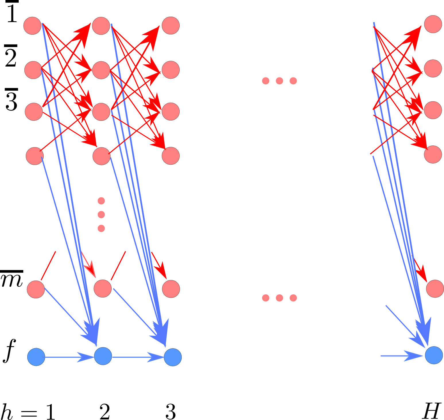
Figure 1: The Leaking Complete Graph Construction. Illustration of a hard MDP. There are $m+1$ states in the MDP, where $f$ is an absorbing terminal state. Starting from any non-terminal state $\overline{a}$, regardless of the action, there is at least $\gamma=1/6$ probability that the next state will be $f$.

The remainder of this section provides the construction of a hard family of MDPs where $Q^{*}$ is linearly realizable and has constant suboptimality gap and where it takes exponential samples to learn a near-optimal policy. Each of these hard MDPs can roughly be seen as a “leaking complete graph” (see Fig. 1). Information about the optimal policy can only be gained by: (1) taking the optimal action; (2) reaching a non-terminal state at level $H$. We will show that when there are exponentially many actions, either events happen with negligible probability unless exponentially many trajectories are played.

4.1 Construction of the MDP family

In this subsection we describe the construction of the hard instance (the hard MDP family) in detail. Let $m$ be an integer to be determined. The state space is $\{\bar{1},\cdots,\bar{m},f\}$. The special state $f$ is called the terminal state. The action space is simply $[m]$. Each MDP in this family is specified by an index $a^{*}\in[m]$ and denoted by $\mathcal{M}_{a^{*}}$. In other words, there are $m$ MDPs in this family.

In order to construct the MDP family, we first find a set of approximately orthogonal vectors by leveraging the Johnson-Lindenstrauss lemma (Johnson and Lindenstrauss, 1984).

Lemma 1 (Johnson-Lindenstrauss).

For any $\gamma>0$, if $m\leq\exp(\frac{1}{8}\gamma^{2}d^{\prime})$, there exists $m$ unit vectors $\{v_{1},\cdots,v_{m}\}$ in $\mathbb{R}^{d^{\prime}}$ such that $\forall i,j\in[m]$ such that $i\neq j$, $|\langle v_{i},v_{j}\rangle|\leq\gamma$.

We will set $\gamma=\frac{1}{6}$ and $m=\lfloor\exp(\frac{1}{8}\gamma^{2}d)\rfloor$. By Lemma 1, we can find such a set of $d$-dimensional unit vectors $\{v_{1},\cdots,v_{m}\}$. For the clarity of presentation, we will use $v_{i}$ and $v(i)$ interchangeably. The construction of $\mathcal{M}_{a^{*}}$ is specified below. Note that in our construction, the features, the rewards and the transitions are defined for all $\overline{a_{1}},a_{2}$ with $a_{1},a_{2}\in[m]$ and $a_{1}\neq a_{2}$. In particular, our construction is properly defined even when $a_{1}=a^{*}$.

Features.

The feature map, which maps state-action pairs to $d+1$ dimensional vectors, is defined as follows.

$$\phi(\overline{a_{1}},a_{2}) :=\left(0,\left(\Big{\langle}v(a_{1}),v(a_{2})\Big{\rangle}+2\gamma\right)\cdot v(a_{2})\right), \forall a_{1},a_{2}\in[m],a_{1}\neq a_{2}$$ ()

$$\phi(\overline{a_{1}},a_{1}) :=\left(\frac{3}{4}\gamma,\mathbf{0}\right), \forall a_{1}\in[m]$$ ()

$$\phi(f,1) =\left(0,\mathbf{0}\right),$$

$$\phi(f,a) :=\left(-1,\mathbf{0}\right). \forall a\neq 1$$ ()

Here $\mathbf{0}$ is the zero vector in $\mathbb{R}^{d}$. Note that the feature map is independent of $a^{*}$ and is shared across the MDP family.

Rewards.

For $1\leq h<H$, the rewards are defined as

$$R_{h}(\overline{a_{1}},a^{*}) :=\Big{\langle}v(a_{1}),v(a^{*})\Big{\rangle}+2\gamma, a_{1}\neq a^{*}$$ ()

$$R_{h}(\overline{a_{1}},a_{2}) :=-2\gamma\left[\Big{\langle}v(a_{1}),v(a_{2})\Big{\rangle}+2\gamma\right], a_{2}\neq a^{*} a_{2}\neq a_{1}$$ (, )

$$R_{h}(\overline{a_{1}},a_{1}) :=\frac{3}{4}\gamma, \forall a_{1}$$ ()

$$R_{h}(f,1) :=0,$$

$$R_{h}(f,a) :=-1. a\neq 1$$ ()

For $h=H$, $r_{H}(s,a):=\langle\phi(s,a),(1,v(a^{*}))\rangle$ for every state-action pair.

Transitions.

The initial state distribution $\mu$ is set as a uniform distribution over $\{\bar{1},\cdots,\bar{m}\}$. The transition probabilities are set as follows.

$$\Pr[f|\overline{a_{1}},a^{*}] =1,$$

$$\Pr[f|\overline{a_{1}},a_{1}] =1,$$

$$\Pr[\cdot|\overline{a_{1}},a_{2}] =\begin{cases}\overline{a_{2}}:\Big{\langle}v(a_{1}),v(a_{2})\Big{\rangle}+2\gamma\\ f:1-\Big{\langle}v(a_{1}),v(a_{2})\Big{\rangle}-2\gamma\end{cases}, a_{2}\neq a^{*} a_{2}\neq a_{1}$$ (, )

$$\Pr[f|f,\cdot] =1.$$

After taking action $a_{2}$, the next state is either $\overline{a_{2}}$ or $f$. Thus this MDP looks roughly like a “leaking complete graph” (see Fig. 1): starting from state $\overline{a}$, it is possible to visit any other state (except for $\overline{a^{*}}$); however, there is always at least $1-3\gamma$ probability of going to the terminal state $f$. The transition probabilities are indeed valid, because

$$0<\gamma\leq\Big{\langle}v(a_{1}),v(a_{2})\Big{\rangle}+2\gamma\leq 3\gamma<1.$$

We now verify that linear realizability, i.e. Assumption 1, is satisfied.

Lemma 2 (Linear realizability).

In the MDP $\mathcal{M}_{a^{*}}$, $\forall h\in[H]$, for any state-action pair $(s,a)$, $Q^{*}_{h}(s,a)=\langle\phi(s,a),\theta^{*}\rangle$ with $\theta^{*}=(1,v(a^{*}))$.

Proof.

We first verify the statement for the terminal state $f$. Observe that at the terminal state $f$, the next state is always $f$ and the reward is either $0$ (if action $1$ is chosen) or $-1$ (if an action other than $1$ is chosen). Hence, we have

$$Q_{h}^{*}(f,a)=\begin{cases}0&a=1\\ -1&a\neq 1\end{cases}$$

and

$$V_{h}^{*}(f)=0.$$

This implies $Q_{h}^{*}(f,\cdot)=\langle\phi(f,\cdot),(1,v(a^{*}))\rangle$.

We now verify realizability for other states via induction on $h=H,H-1,\cdots,1$. The induction hypothesis is that for all $a_{1},a_{2}\in[m]$, we have

$$Q_{h}^{*}(\overline{a_{1}},{a_{2}})=\begin{cases}\left(\left\langle v(a_{1}),v(a_{2})\right\rangle+2\gamma\right)\cdot\left\langle v(a_{2}),v(a^{*})\right\rangle&a_{1}\neq a_{2}\\ \frac{3}{4}\gamma&a_{1}=a_{2}\end{cases}$$ (1)

and

$$V_{h}^{*}(\overline{a_{1}})=\begin{cases}\left\langle v(a_{1}),v(a^{*})\right\rangle+2\gamma&a_{1}\neq a^{*}\\ \frac{3}{4}\gamma&a_{1}=a^{*}\end{cases}.$$ (2)

Note that (1) implies that realizability is satisfied. In the remaining part of the proof we verify Eq. (1) and (2).

When $h=H$, (1) holds by the definition of rewards. Next, note that for all $h\in[H]$, (2) follows from (1). This is because for all $a_{1}\neq a^{*}$, for all $a_{2}\notin\{a_{1},a^{*}\}$.

$$Q_{h}^{*}(\overline{a_{1}},{a_{2}}) =\left(\left\langle v(a_{1}),v(a_{2})\right\rangle+2\gamma\right)\cdot\left\langle v(a_{2}),v(a^{*})\right\rangle\leq 3\gamma^{2},$$

Moreover, for all $a_{1}\neq a^{*}$,

$$Q_{h}^{*}(\overline{a_{1}},{a_{1}}) =\frac{3}{4}\gamma<\gamma.$$

Furthermore, for all $a_{1}\neq a^{*}$,

$$Q_{h}^{*}(\overline{a_{1}},{a^{*}})=\left\langle v(a_{1}),v(a^{*})\right\rangle+2\gamma\geq\gamma>3\gamma^{2}.$$

In other words, (1) implies that $a^{*}$ is always the optimal action for all state $\overline{a_{1}}$ with $a_{1}\neq a^{*}$. Now, for state $\overline{a^{*}}$, for all $a\neq a^{*}$, we have

$$Q_{h}^{*}(\overline{a^{*}},a) =\left(\left\langle v(a^{*}),v(a)\right\rangle+2\gamma\right)\cdot\left\langle v(a^{*}),v(a)\right\rangle\leq 3\gamma^{2}<\frac{3}{4}\gamma=Q_{h}^{*}(\overline{a^{*}},a^{*}).$$

Hence, (1) implies that $a^{*}$ is always the optimal action for all states $\overline{a}$ with $a\in[m]$.

Thus, it remains to show that (1) holds for $h$ assuming (2) holds for $h+1$. Here we only consider the case that $a_{2}\neq a_{1}$ and $a_{2}\neq a^{*}$, since otherwise $\Pr[f|\overline{a_{1}},a_{2}]=1$ and thus (1) holds by the definition of the rewards and the fact that $V_{h}^{*}(f)=0$. When $a_{2}\notin\{a_{1},a^{*}\}$, we have

$$Q_{h}^{*}(\overline{a_{1}},{a_{2}}) =R_{h}(\overline{a_{1}},a_{2})+\mathbb{E}_{s_{h+1}}\left[\left.V_{h+1}^{*}(s_{h+1})\right|\overline{a_{1}},a_{2}\right]$$

$$=-2\gamma\left[\Big{\langle}v(a_{1}),v(a_{2})\Big{\rangle}+2\gamma\right]+\Pr[s_{h+1}=\overline{a_{2}}]\cdot V_{h+1}^{*}(a_{2})+\Pr[s_{h+1}=f]\cdot V_{h+1}^{*}(f)$$

$$=-2\gamma\left[\Big{\langle}v(a_{1}),v(a_{2})\Big{\rangle}+2\gamma\right]+\left[\Big{\langle}v(a_{1}),v(a_{2})\Big{\rangle}+2\gamma\right]\cdot\left(\Big{\langle}v(a_{1}),v(a^{*})\Big{\rangle}+2\gamma\right)$$

$$=\left(\Big{\langle}v(a_{1}),v(a_{2})\Big{\rangle}+2\gamma\right)\cdot\Big{\langle}v(a_{1}),v(a^{*})\Big{\rangle}.$$

This is exactly (1) for $h$. Hence both (1) and (2) hold for all $h\in[H]$. ∎

We now verify that the minimum suboptimality gap $\Delta_{\min}$ is lower bounded.

Lemma 3 (Constant gap).

Assumption 2 is satisfied with $\Delta_{\min}=\frac{1}{24}$.

Proof.

From Eq. (1) and (2), it is easy to see that at state $\overline{a_{1}}\neq\overline{a^{*}}$, for $a_{2}\neq a^{*}$, the suboptimality gap is

$$\Delta_{h}(\overline{a_{1}},a_{2}):=V_{h}^{*}(\overline{a_{1}})-Q^{*}_{h}(\overline{a_{1}},a_{2})\geq\gamma-\max\left\{3\gamma^{2},\frac{3}{4}\gamma\right\}=\frac{1}{24}.$$

Moreover, at state $\overline{a^{*}}$, for $a\neq a^{*}$, the suboptimality gap is

$$\Delta_{h}(\overline{a^{*}},a):=V_{h}^{*}(\overline{a^{*}})-Q^{*}_{h}(\overline{a^{*}},a)\geq\frac{3}{4}\gamma-3\gamma^{2}=\frac{1}{24}.$$

Finally, for the terminal state $f$, the suboptimality gap is obviously $1$. Therefore $\Delta_{\min}\geq\frac{1}{24}$ for all MDPs under consideration. ∎

4.2 The information-theoretic argument

Now we are ready to state and prove our main technical lemma.

Lemma 4.

For any algorithm, there exists $a^{*}\in[m]$ such that in order to output $\pi$ with

$$\mathbb{E}_{s_{1}\sim\mu}V^{\pi}(s_{1})\geq\mathbb{E}_{s_{1}\sim\mu}V^{*}(s_{1})-0.05$$

with probability at least $0.1$ for $\mathcal{M}_{a^{*}}$, the number of samples required is $2^{\Omega(\min\{d,H\})}$.

We provide a proof sketch for the lower bound below. The full proof can be found in Appendix B. Our main result, Theorem 1, is a direct consequence of Lemma 4.

Proof sketch.

Observe that the feature map of $\mathcal{M}_{a^{*}}$ does not depend on $a^{*}$, and that for $h<H$ and $a_{2}\neq a^{*}$, the reward $R_{h}(\overline{a_{1}},a_{2})$ also contains no information about $a^{*}$. The transition probabilities are also independent of $a^{*}$, unless the action $a^{*}$ is taken. Moreover, the reward at state $f$ is always $0$. Thus, to receive information about $a^{*}$, the agent either needs to take the action $a^{*}$, or be at a non-game-over state at the final time step ($h=H$).

However, note that the probability of remaining at a non-terminal state at the next layer is at most

$$\sup_{a_{1}\neq a_{2}}\langle v(a_{1}),v(a_{2})\rangle+2\gamma\leq 3\gamma\leq\frac{3}{4}.$$

Thus for any algorithm, $\Pr[s_{H}\neq f]\leq\left(\frac{3}{4}\right)^{H}$, which is exponentially small.

In other words, any algorithm that does not know $a^{*}$ either needs to “be lucky” so that $s_{H}=f$, or needs to take $a^{*}$ “by accident”. Since the number of actions is $m=2^{\Theta(d)}$, either event cannot happen with constant probability unless the number of episodes is exponential in $\min\{d,H\}$.

In order to make this claim rigorous, we can construct a reference MDP $\mathcal{M}_{0}$ as follows. The state space, action space, and features of $\mathcal{M}_{0}$ are the same as those of $\mathcal{M}_{a}$. The transitions are defined as follows:

$$\Pr[\cdot|\overline{a_{1}},a_{2}] =\begin{cases}\overline{a_{2}}:\Big{\langle}v(a_{1}),v(a_{2})\Big{\rangle}+2\gamma\\ f:1-\Big{\langle}v(a_{1}),v(a_{2})\Big{\rangle}-2\gamma\end{cases}, \forall a_{1},a_{2} a_{1}\neq a_{2}$$ ( s.t. )

$$\Pr[f|f,\cdot] =1.$$

The rewards are defined as follows:

$$R_{h}(\overline{a_{1}},a_{2}) :=-2\gamma\left[\Big{\langle}v(a_{1}),v(a_{2})\Big{\rangle}+2\gamma\right], \forall a_{1},a_{2} a_{1}\neq a_{2}$$ ( s.t. )

$$R_{h}(f,\cdot) :=0.$$

Note that $\mathcal{M}_{0}$ is identical to $\mathcal{M}_{a^{*}}$, except when $a^{*}$ is taken, or when an trajectory ends at a non-terminal state. Since the latter event happens with an exponentially small probability, we can show that for any algorithm the probability of taking $a^{*}$ in $\mathcal{M}_{a^{*}}$ is close to the probability of taking $a^{*}$ in $\mathcal{M}_{0}$. Since $\mathcal{M}_{0}$ is independent of $a^{*}$, unless an exponential number of samples are used, for any algorithm there exists $a^{*}\in[m]$ such that the probability of taking $a^{*}$ in $\mathcal{M}_{0}$ is $o(1)$. It then follows that the probability of taking $a^{*}$ in $\mathcal{M}_{a^{*}}$ is $o(1)$. Since $a^{*}$ is the optimal action for every state, such an algorithm cannot output a near-optimal policy for $\mathcal{M}_{a^{*}}$.

5 Upper Bound

Theorem 1 suggests that Assumption 1 and Assumption 2 are not sufficient for sample-efficient RL when the number of actions could be exponential, and that additional assumptions are needed to achieve polynomial sample complexity. One style of assumption is via assuming a global representation property on the features, such as completeness (Zanette et al., 2020).

In this section, we consider two assumptions on additional structures on the transitions of the MDP rather than the feature representation that enable good rates for linear regression with sparse bias. The first condition is a variant of the low variance condition in Du et al. (2019c).

Assumption 3 (Low variance condition).

There exists a constant $1\leq C_{\mathrm{var}}<\infty$ such that for any $h\in[H]$ and any policy $\pi$,

$$\mathbb{E}_{s\sim\mathcal{D}^{\pi}_{h}}\left[\left|V^{\pi}(s)-V^{*}(s)\right|^{2}\right]\leq C_{\mathrm{var}}\cdot\left(\mathbb{E}_{s\sim\mathcal{D}^{\pi}_{h}}\left[\left|V^{\pi}(s)-V^{*}(s)\right|\right]\right)^{2}.$$

We also consider an alternative assumption where feature distribution is hypercontractive.

Assumption 4.

(Hypercontractivity of $\phi$) There exists a constant $1\leq C_{\mathrm{hyper}}<\infty$ such that for any $h\in[H]$ and any policy $\pi$, the distribution of $\phi(s,a)$ with $(s,a)\sim\mathcal{D}^{\pi}_{h}$ is $(C_{\mathrm{hyper}},4)$-hypercontractive. In other words, $\forall\pi$, $\forall h\in[H]$, $\forall v\in\mathbb{R}^{d}$,

$$\mathbb{E}_{(s,a)\sim\mathcal{D}^{\pi}_{h}}\left[(\phi(s,a)^{\top}v)^{4}\right]\leq C_{\mathrm{hyper}}\cdot\left(\mathbb{E}_{(s,a)\sim\mathcal{D}^{\pi}_{h}}[(\phi(s,a)^{\top}v)^{2}]\right)^{2}.$$

Intuitively, hypercontractivity characterizes the anti-concentration of a distribution. A broad class of distributions are hypercontractive with $C_{\mathrm{hyper}}=O(1)$, including Gaussian distributions (of arbitrary covariance matrices), uniform distributions over the hypercube and sphere, and strongly log-concave distributions (Kothari and Steurer, 2017). Hypercontractivity has been previously used for outlier-robust linear regression (Klivans et al., 2018; Bakshi and Prasad, 2020) and moment-estimation (Kothari and Steurer, 2017).

We show that under Assumptions 1, 2, 3 or  1, 2, 4, a modified version of the Difference Maximization Q-learning (DMQ) algorithm (Du et al., 2019c) is able to learn a near-optimal policy using polynomial number of trajectories with no dependency on the number of actions.

5.1 Optimal experiment design

Given a set of $d$-dimensional vectors, (optimal) experiment design aims at finding a distribution $\rho$ over the vectors such that when sampling from this distribution, linear regression performs optimally based on some criteria. In this paper, we will use the G-optimality criterion, which minimizes the maximum prediction variance over the set. The following lemma on G-optimal design is a direct corollary of the Kiefer-Wolfowitz theorem (Kiefer and Wolfowitz, 1960).

Lemma 5 (Existence of G-optimal design).

For any set $X\subseteq\mathbb{R}^{d}$, there exists a distribution $\mathcal{K}_{X}$ supported on $X$, known as the G-optimal design, such that

$$\max_{x\in X}x^{\top}\left(\mathbb{E}_{z\sim\mathcal{K}_{X}}zz^{\top}\right)^{-1}x\leq d.$$

Efficient algorithms for finding such a distribution can be found in Todd (2016).

In the context of reinforcement learning, the set $X$ corresponds to the set of all features, which is inaccessible. Instead, one can only observe one state $s$ at a time, and choose $a\in\mathcal{A}$ based on the features $\{\phi(s,a)\}_{a\in\mathcal{A}}$. Such a problem is closer to the distributional optimal design problem described by Ruan et al. (2020). For our purpose, the following simple approach suffices: given a state $s$, perform exploration by sampling from the G-optimal design on $\{\phi(s,a)\}_{a\in\mathcal{A}}$. The performance of this exploration strategy is guaranteed by the following lemma, which will be used in the analysis in Section 5.

Lemma 6 (Lemma 4 in Ruan et al. (2020)).

For any state $s$, denote the $G$-optimal design with its features by $\rho_{s}(\cdot)\in\Delta_{A}$, and the corresponding covariance matrix by $\Sigma_{s}:=\sum_{a}\rho_{s}(a)\phi(s,a)\phi(s,a)^{\top}$. Given a distribution $\nu$ over states. Denote the average covariance matrix by $\Sigma:=\mathbb{E}_{s\sim\nu}\Sigma_{s}$. Then

$$\mathbb{E}_{s\sim\nu}\left[\max_{a\in\mathcal{A}}\phi(s,a)^{\top}\Sigma^{-1}\phi(s,a)\right]\leq d^{2}.$$

We provide a proof in the appendix for completeness.

Note that the performance of this strategy is only worse by a factor of $d$ (compared to the case where one can query all features), and has no dependency on the number of actions.

5.2 The modified DMQ algorithm

Overview.

During the execution of the Difference Maximization Q-learning (DMQ) algorithm, for each level $h\in[H]$, we maintain three variables: the estimated linear coefficients $\theta_{h}\in\mathbb{R}^{d}$, a set of exploratory policies $\Pi_{h}$, and the empirical feature covariance matrix $\Sigma_{h}$ associated with $\Pi_{h}$. We initialize $\theta_{h}=\mathbf{0}\in\mathbb{R}^{d}$, $\Sigma_{h}:=\mathbf{0}_{d\times d}$ and $\Pi_{h}$ to as a single purely random exploration policy, i.e., $\Pi_{h}=\{\pi\}$ where $\pi$ chooses an action uniformly at random for all states.

Each time we execute Algorithm 1, the goal is to update the estimated linear coefficients $\theta_{h}\in\mathbb{R}^{d}$, so that for all $\pi\in\Pi_{h}$, $\theta_{h}$ is a good estimation to $\theta_{h}^{*}$ with respect to the distribution induced by $\pi$. We run ridge regression on the data distribution induced by policies in $\Pi_{h}$, and the regression targets are collected by invoking the greedy policy induced by $\{\theta_{h^{\prime}}\}_{h^{\prime}>h}$.

However, there are two apparent issues with such an approach. First, for levels $h^{\prime}>h$, $\theta_{h^{\prime}}$ is guaranteed to achieve low estimation error only with respect to the distributions induced by policies $\Pi_{h^{\prime}}$. It is possible that for some $\pi\in\Pi_{h}$, the estimation error of $\theta_{h^{\prime}}$ is high for the distribution induced by $\pi$ (followed by the greedy policy). To resolve this issue, the main idea in Du et al. (2019c) is to explicitly check whether $\theta_{h^{\prime}}$ also predicts well on the new distribution (see Line 1 in Algorithm 1). If not, we add the new policy into $\Pi_{h^{\prime}}$ and invoke Algorithm 1 recursively. The analysis in Du et al. (2019c) upper bounds the total number of recursive calls by a potential function argument, which also gives an upper bound on the sample complexity of the algorithm.

Second, the exploratory policies $\Pi_{h}$ only induce a distribution over states at level $h$, and the algorithm still needs to decide an exploration strategy to choose actions at level $h$. To this end, the algorithm in Du et al. (2019c) explores all actions uniformly at random, and therefore the sample complexity has at least linear dependency on the number of actions. We note that similar issues also appear in the linear contextual bandit literature (Lattimore and Szepesvári, 2020; Ruan et al., 2020), and indeed our solution here is to explore by sampling from the G-optimal design over the features at a single state. As shown by Lemma 6, for all possible roll-in distributions, such an exploration strategy achieves a nice coverage over the feature space, and is therefore sufficient for eliminating the dependency on the size of the action space.

Input: A level $h\in\{0,\cdots,H\}$

1 for $\pi_{h}\in\Pi_{h}$ do

2       for $h^{\prime}=H,H-1,\cdots,h+1$ do

3             Collect $N$ samples $\{(s_{h^{\prime}}^{j},a_{h^{\prime}}^{j})\}_{j\in[N]}$ with $s_{h^{\prime}}^{j}\sim\mathcal{D}^{\tilde{\pi}_{h}}_{h^{\prime}}$ and $a_{h^{\prime}}^{j}\sim\rho_{s_{h^{\prime}}^{j}}$ ($\tilde{\pi}_{h}$ defined in (3))

4             $\hat{\Sigma}_{h^{\prime}}\leftarrow\frac{1}{N}\sum_{j=1}^{N}\phi(s_{h^{\prime}}^{j},a_{h^{\prime}}^{j})\phi(s_{h^{\prime}}^{j},a_{h^{\prime}}^{j})^{\top}$

5             if $\|\Sigma_{h^{\prime}}^{-\frac{1}{2}}\hat{\Sigma}_{h^{\prime}}\Sigma_{h^{\prime}}^{-\frac{1}{2}}\|_{2}>\beta|\Pi_{h^{\prime}}|$ then

6                  

7                  $\Pi_{h^{\prime}}\leftarrow\Pi_{h^{\prime}}\cup\{\tilde{\pi}_{h}\}$

8                   Run LearnLevel recursively on level $h^{\prime}$

9                   Goto Line $1$ (restart the algorithm)

10            

11      

12if $h=0$ then

13       Output greedy policy with respect to $\{\theta_{h}\}_{h\in[H]}$

14      

15$\Sigma_{h}\leftarrow\frac{\lambda_{r}}{|\Pi_{h}|}I$,$\quad w_{h}\leftarrow\mathbf{0}\in\mathbb{R}^{d}$

16 for $i=1,\cdots,N\left|\Pi_{h}\right|$ do

17       Sample $\pi$ from uniform distribution over $\Pi_{h}$

18       Execute $\tilde{\pi}_{h}$ (see (3)) to collect $(s^{i}_{h},a^{i}_{h},y_{i})$, where $y_{i}:=\sum_{h^{\prime}\geq h}r^{i}_{h^{\prime}}$ is the on-the-go reward

19       $\Sigma_{h}\leftarrow\Sigma_{h}+\frac{1}{N|\Pi_{h}|}\phi(s^{i}_{h},a^{i}_{h})\phi(s^{i}_{h},a^{i}_{h})^{\top}$

20       $w_{h}\leftarrow w_{h}+\frac{1}{N|\Pi_{h}|}\phi(s^{i}_{h},a^{i}_{h})y_{i}$

21$\theta_{h}\leftarrow\left((\lambda_{\rm ridge}-\frac{\lambda_{r}}{|\Pi_{h}|})I+\Sigma_{h}\right)^{-1}w_{h}$

Algorithm 1 LearnLevel

The algorithm.

The formal description of the algorithm is given in Algorithm 1. The algorithm should be run by calling LearnLevel on input $h=0$.

Here, for a policy $\pi_{h}\in\Pi_{h}$, the associated exploratory policy $\tilde{\pi}_{h}$ is defined as

$$\tilde{\pi}_{h}(s_{h^{\prime}})=\begin{cases}\pi(s_{h^{\prime}})&(\text{if }h^{\prime}<h)\\ \text{Sample from }\rho_{s_{h}}(\cdot)&(\text{if }h^{\prime}=h)\\ \arg\max_{a}\phi_{h^{\prime}}(s_{h^{\prime}},a)^{\top}\theta_{h^{\prime}}&(\text{if }h^{\prime}>h)\\ \end{cases}.$$ (3)

Here $\rho_{s}(\cdot)$ is the G-optimal design on the set of vectors $\{\phi(s,\cdot)\}_{a\in\mathcal{A}}$, as defined by Lemma 5. Note that when $h=0$, $\tilde{\pi}_{h}$ is always the greedy policy on $\{\theta_{h}\}_{h\in[H]}$. The choice of the algorithmic parameters ($\beta$, $\lambda_{r}$, $\lambda_{\rm ridge}$) can be found in the proof of Theorem 2.

5.3 Analysis

We show the following theorem regarding the modified algorithm.

Theorem 2.

Assume that Assumption 1, 2 and one of Assumption 3 and 4 hold. Also assume that

$$\epsilon \leq\mathrm{poly}(\Delta_{\min},1/C_{\mathrm{var}},1/d,1/H)$$ (Under Assumption 3)

$${\rm or}\quad\epsilon \leq\mathrm{poly}(\Delta_{\min},1/C_{\mathrm{hyper}},1/d,1/H).$$ (Under Assumption 4)

Let $\mu$ be the initial state distribution. Then with probability $1-\epsilon$, running Algorithm 1 on input $0$ returns a policy $\pi$ which satisfies $\mathbb{E}_{s_{1}\sim\mu}V^{\pi}(s_{1})\geq\mathbb{E}_{s_{1}\sim\mu}V^{*}(s_{1})-\epsilon$ using $\mathrm{poly}(1/\epsilon)$ trajectories.

Note that here both the algorithm and the theorem have no dependence on $A$, the number of actions. The proof of the theorem under Assumption 3 is largely based on the analysis in Du et al. (2019c). The largest difference is that we used Lemma 6 instead of the original union bound argument when controlling $\Pr\left[\sup_{a}|\theta_{h}^{\top}\phi(s,a)Q_{h}^{*}(s,a)|>\frac{\gamma}{2}\right]$. The proof under Assumption 4 relies on a novel analysis of least squares regression under hypercontractivity. The full proof is deferred to Appendix D.

6 Discussion

Exponential separation between the generative model and the online setting.

When a generative model (also known as simulator) is available, Assumption 1 and Assumption 2 are sufficient for designing an algorithm with $\mathrm{poly}(1/\epsilon,1/\Delta_{\min},d,H)$ sample complexity (Du et al., 2019b, Theorem C.1). As shown by Theorem 1, under the standard online RL setting (i.e. without access to a generative model), the sample complexity is lower bounded by $2^{\Omega(\min\{d,H\})}$ when $\Delta_{\min}=\Theta(1)$, under the same set of assumptions. This implies that the generative model is exponentially more powerful than the standard online RL setting.

Although the generative model is conceptually much stronger than the online RL model, previously little is known on the extent to which the former is more powerful. In tabular RL, for instance, the known sample complexity bounds with or without access to generative models are nearly the same (Zhang et al., 2020; Agarwal et al., 2020), and both match the lower bound (up to logarithmic factors). To the best of our knowledge, the only existing example of such separation is shown by Wang et al. (2020a) under the following set of conditions: (i) deterministic system; (ii) realizability (Assumption 1); (iii) no reward feedback (a.k.a. reward-free exploration). In comparison, our separation result holds under less restrictions (allows stochasticity) and for the usual RL environment (instead of reward-free exploration), and it therefore far more natural.

Connecting Theorem 1 and Theorem 2.

Our hardness result in Theorem 1 shows that under Assumption 1 and Assumption 2, any algorithm requires exponential number of samples to find a near-optimal policy, and therefore, sample-efficient RL is impossible without further assumptions (e.g., Assumption 3 or Assumption 4 assumed in Theorem 2). Indeed, Theorem 1 and Theorem 2 imply that the coefficient $C$ in Assumption 3 and $C_{\mathrm{hyper}}$ in Assumption 4 is at least exponential for the hard MDP family used in Theorem 1. In fact, the subtlety here is that $C$ in Assumption 3 and $C_{\mathrm{hyper}}$ in Assumption 4 need to be upper bounded for all policies $\pi$. It can be easily verified that for the hard MDP family used in Theorem 1, for some policy $\pi$, $C$ in Assumption 3 and $C_{\mathrm{hyper}}$ in Assumption 4 is exponential.

Minimum reaching probability.

We would also like to mention the following reachability condition, which is assumed by Du et al. (2019a); Misra et al. (2020). Denote the probability under policy $\pi$ of visiting state $s$ at step $h$ by $\Pr^{\pi}_{h}[s]$; then it is assumed that $\min_{s\in\mathcal{S},h>1}\max_{\pi}\Pr^{\pi}_{h}[s]=\eta_{\min}>0$. Although in $\mathcal{M}_{a^{*}}$, $\eta_{\min}\leq 2^{-\Theta(H)}$ is exponentially small, one can slightly modify the construction so that $\eta_{\min}=1$ (see Appendix C for details). The rationale is straightforward: in the $\mathcal{M}_{a^{*}}$, the action $a^{*}$ will not be taken with high probability in polynomial samples. Thus, one can exploit this by setting $a^{*}$ to lead to a special state from which all states are reachable. This suggests that even under Assumption 1, Assumption 2 and the condition that $\eta_{\min}=1$, there is an exponential sample complexity lower bound.

Open problems.

The first open problem, perhaps an obvious one, is whether a sample complexity lower bound under Assumption 1 can be shown with polynomial number of actions. This will further rule out $\mathrm{poly}(A,d,H)$-style upper bounds, which are still possible with the current results. An even stronger lower bound would be one with polynomial number of actions under both realizability and minimum suboptimality gap. Such lower bound will likely settle the sample complexity of reinforcement learning with linear function approximation under the realizability assumption. Another open problem is whether Assumption 3 and 4 can be replaced by or understood as more natural characterizations of the complexity of the MDP.

Appendix A Proof of Lemma 6

Proof.

We state a proof of this lemma for completeness. By Lemma 5, $\forall s$,

$$\max_{a\in\mathcal{A}}\phi(s,a)^{\top}\Sigma_{s}^{-1}\phi(s,a)\leq d.$$

It follows that $\forall a\in\mathcal{A}$,

$$\phi(s,a)\phi(s,a)^{\top}\preccurlyeq d\Sigma_{s}.$$

Therefore,

$$\mathbb{E}_{s\sim\nu}\left[\max_{a\in\mathcal{A}}\phi(s,a)^{\top}\Sigma^{-1}\phi(s,a)\right] =\mathbb{E}_{s\sim\nu}\max_{a\in\mathcal{A}}{\rm Tr}\left(\phi(s,a)\phi(s,a)^{\top}\Sigma^{-1}\right)$$

$$\leq\mathbb{E}_{s\sim\nu}{\rm Tr}\left(d\Sigma_{s}\Sigma^{-1}\right)=d^{2}.$$

∎

Appendix B Proof of Theorem 1

Proof.

We consider $K$ episodes of interaction between the algorithm and the MDP $\mathcal{M}_{a}$. Since each trajectory is a sequence of $H$ states, we define the total number of samples as $KH$. Denote the state, the action and the reward at episode $k$ and timestep $h$ by $s^{k}_{h}$, $a^{k}_{h}$ and $r^{k}_{h}$ respectively.

Consider the following reference MDP denoted by $\mathcal{M}_{0}$. The state space, action space, and features of this MDP are the same as those of the MDP family. The transitions are defined as follows:

$$\Pr[\cdot|\overline{a_{1}},a_{2}] =\begin{cases}\overline{a_{2}}:\Big{\langle}v(a_{1}),v(a_{2})\Big{\rangle}+2\gamma\\ f:1-\Big{\langle}v(a_{1}),v(a_{2})\Big{\rangle}-2\gamma\end{cases}, \forall a_{1},a_{2} a_{1}\neq a_{2}$$ ( s.t. )

$$\Pr[f|f,\cdot] =1.$$

The rewards are defined as follows:

$$R_{h}(\overline{a_{1}},a_{2}) :=-2\gamma\left[\Big{\langle}v(a_{1}),v(a_{2})\Big{\rangle}+2\gamma\right], \forall a_{1},a_{2} a_{1}\neq a_{2}$$ ( s.t. )

$$R_{h}(f,\cdot) :=0.$$

Intuitively, this MDP is very similar to the MDP family, except that the optimal action $a^{*}$ is removed. More specifically, $\mathcal{M}_{0}$ is identical to $\mathcal{M}_{a}$ except when the action $a$ is taken at a non-terminal state, or when an episode ends at a non-terminal state.

More specifically, we claim that for $t<H$, $\forall s_{t},a_{t}$ such that $a_{t}\neq a$,

$$\mathrm{Pr}_{\mathcal{M}_{a}}[s_{t+1}|s_{t},a_{t}]=\mathrm{Pr}_{\mathcal{M}_{0}}[s_{t+1}|s_{t},a_{t}],$$

and that for $t<H$, $\forall s_{t},a_{t}$ such that $a_{t}\neq a$,

$$r_{t}^{\mathcal{M}_{a}}(s_{t},a_{t})=r_{t}^{\mathcal{M}_{0}}(s_{t},a_{t}).$$

Also, $r_{H}^{\mathcal{M}_{a}}(s_{t},a_{t})=r_{H}^{\mathcal{M}_{0}}(s_{t},a_{t})$ if $s_{t}=f$. It follows that

$$\mathrm{Pr}_{\mathcal{M}_{a}}\left[s^{1}_{1},a^{1}_{1},r^{1}_{1},\cdots s^{k}_{h},a^{k}_{h},r^{k}_{h}\left|a\notin A^{k}_{h},\forall k^{\prime}\leq k,s^{k^{\prime}}_{H}=f\right.\right]$$

$$= \mathrm{Pr}_{\mathcal{M}_{0}}\left[s^{1}_{1},a^{1}_{1},r^{1}_{1},\cdots s^{k}_{h},a^{k}_{h},r^{k}_{h}\left|a\notin A^{k}_{h},\forall k^{\prime}\leq k,s^{k^{\prime}}_{H}=f\right.\right].$$

Here $A^{k}_{h}$ is a shorthand for $\left\{a^{1}_{1},a^{1}_{2},\cdots,a^{1}_{H},\cdots,a^{k}_{h}\right\}$, i.e. all actions taken up to timestep $h$ for episode $k$. By marginalizing the states and the actions, we get

$$\mathrm{Pr}_{\mathcal{M}_{a}}\left[a^{k}_{h}\left|a\notin A^{k}_{h},\forall k^{\prime}\leq k,s^{k^{\prime}}_{H}=f\right.\right]=\mathrm{Pr}_{\mathcal{M}_{0}}\left[a^{k}_{h}\left|a\notin A^{k}_{h},\forall k^{\prime}\leq k,s^{k^{\prime}}_{H}=f\right.\right].$$

It then follows that

$$\mathrm{Pr}_{\mathcal{M}_{a}}\left[a^{k}_{h}=a\left|a\notin A^{k}_{h},\forall k^{\prime}\leq k,s^{k^{\prime}}_{H}=f\right.\right]=\mathrm{Pr}_{\mathcal{M}_{0}}\left[a^{k}_{h}=a\left|a\notin A^{k}_{h},\forall k^{\prime}\leq k,s^{k^{\prime}}_{H}=f\right.\right].$$

Next, we prove via induction that

$$\mathrm{Pr}_{\mathcal{M}_{a}}\left[a\in A^{k}_{h}\left|\forall k^{\prime}\leq k,s^{k^{\prime}}_{H}=f\right.\right]=\mathrm{Pr}_{\mathcal{M}_{0}}\left[a\in A^{k}_{h}\left|\forall k^{\prime}\leq k,s^{k^{\prime}}_{H}=f\right.\right].$$ (4)

Suppose that (4) holds up to $(k,h-1)$. Then

$$\mathrm{Pr}_{\mathcal{M}_{a}}\left[a\in A^{k}_{h}\left|\forall k^{\prime}\leq k,s^{k^{\prime}}_{H}=f\right.\right]$$

$$= \mathrm{Pr}_{\mathcal{M}_{a}}\left[a\notin A^{k}_{h-1}\right]\mathrm{Pr}_{\mathcal{M}_{a}}\left[a^{k}_{h}=a\left|a\notin A^{k}_{h-1},\forall k^{\prime}\leq k,s^{k^{\prime}}_{H}=f\right.\right]+\mathrm{Pr}_{\mathcal{M}_{a}}\left[a\in A^{k}_{h-1}\left|\forall k^{\prime}\leq k,s^{k^{\prime}}_{H}=f\right.\right]$$

$$= \mathrm{Pr}_{\mathcal{M}_{0}}\left[a\notin A^{k}_{h-1}\right]\mathrm{Pr}_{\mathcal{M}_{0}}\left[a^{k}_{h}=a\left|a\notin A^{k}_{h-1},\forall k^{\prime}\leq k,s^{k^{\prime}}_{H}=f\right.\right]+\mathrm{Pr}_{\mathcal{M}_{0}}\left[a\in A^{k}_{h-1}\left|\forall k^{\prime}\leq k,s^{k^{\prime}}_{H}=f\right.\right]$$

$$= \mathrm{Pr}_{\mathcal{M}_{0}}\left[a\in A^{k}_{h}\left|\forall k^{\prime}\leq k,s^{k^{\prime}}_{H}=f\right.\right].$$

That is, (4) holds for $h$, $k$ as well. By induction, (4) holds for all $h$, $k$. Thus,

$$\mathrm{Pr}_{\mathcal{M}_{a}}\left[a\in A^{k}_{h}\right] \leq\mathrm{Pr}_{\mathcal{M}_{a}}\left[a\in A^{k}_{h}\left|\forall k^{\prime}\leq k,s^{k^{\prime}}_{H}=f\right.\right]+\Pr\left[\exists k^{\prime}\leq k,s^{k^{\prime}}_{H}\neq f\right]$$

$$\leq\mathrm{Pr}_{\mathcal{M}_{0}}\left[a\in A^{k}_{h}\left|\forall k^{\prime}\leq k,s^{k^{\prime}}_{H}=f\right.\right]+k\cdot\left(\frac{3}{4}\right)^{H}.$$

Since $|A^{k}_{h}|\leq kH$, $\sum_{a\in[m]}\mathrm{Pr}_{\mathcal{M}_{0}}\left[a\in A^{k}_{h}\left|\forall k^{\prime}\leq k,s^{k^{\prime}}_{H}=f\right.\right]\leq kH$. It follows that there exists $a^{*}\in[m]$ such that

$$\mathrm{Pr}_{\mathcal{M}_{0}}\left[a^{*}\in A^{K}_{H}\left|\forall k^{\prime}\leq K,s^{k^{\prime}}_{H}=f\right.\right]\leq\frac{KH}{m}.$$

As a result

$$\mathrm{Pr}_{\mathcal{M}_{a^{*}}}\left[a^{*}\in A^{K}_{H}\right]\leq\frac{KH}{m}+K\left(\frac{3}{4}\right)^{H}.$$

Recall that $m=\lfloor\exp(\frac{1}{8}\gamma^{2}d)\rfloor$ and $\gamma=\frac{1}{6}$. Therefore, unless $KH=2^{\Omega\left(\min\{d,H\}\right)}$, the probability of taking the optimal action $a^{*}$ in the interaction with $\mathcal{M}_{a^{*}}$ is $o(1)$.

From the suboptimality gap condition, it follows that if $\mathbb{E}_{s_{1}\sim\mu}V^{\pi}(s_{1})\geq\mathbb{E}_{s_{1}\sim\mu}V^{*}(s_{1})-0.05$, $\Pr\left[a_{1}\neq a^{*}\land s_{1}\neq\overline{a^{*}}\right]\cdot\Delta_{\min}\leq 0.05$. Hence

$$\Pr\left[a_{1}=a^{*}\right]\geq 1-\left(0.8+\frac{1}{m}\right)=0.2-\frac{1}{m}.$$

Therefore, if the algorithm is able to output such a policy with probability $0.1$, it is able to take the action $a^{*}$ in the next episode with $\Theta(1)$ probability by executing $\pi$. However, as proved above, this is impossible unless $KH=2^{\Omega\left(\min\{d,H\}\right)}$. ∎

Appendix C Ensuring Minimum Reachability

As mentioned in Section 6, the hardness results holds even when all states can be reached with probability $1$. In this section, we demonstrate how to modify the construction in Section 4 so that all states can be reached with probability $1$.

Based on the construction in Section 4, we will modify $\mathcal{M}_{a^{*}}$ in the following manner.

1. Remove the state $\overline{a^{*}}$.

2. Create a deterministic initial state $s$; at state $s$, taking action $a\neq a^{*}$ leads to state $\overline{a}$; taking a special action $0$ leads to the terminal state $f$; taking action $a^{*}$ leads to state $s$ again.

3. Set $\phi(s,0)=(-1,\mathbf{0}$); $\phi(s,a)=(-1,v(a))$.

4. $R(s,a)=-1-2\gamma$ for $a\in[m]\neq a^{*}$. $R(s,a^{*})=0$. $R(s,0)=-1$.

It can be seen that now, $\eta_{\min}=1$ because to reach state $\overline{a}$ at level $h$, one can simply take the action sequence $a^{*},\cdots,a^{*},a$. Realizability at the initial state $s$ can also be verified (with $\theta^{*}=(1,v(a^{*}))$ as before).

Appendix D Proof of Theorem 2

Proof under Assumption 3.

Let us set $\beta=8$, $\lambda_{\rm ridge}=\epsilon^{2}$, $\lambda_{r}=\epsilon^{6}$, $B=2d\log(\frac{d}{\lambda_{r}})$, $\epsilon_{1}=\epsilon^{2}$, $\epsilon_{2}=\frac{\lambda_{r}}{2B}$, $N=\frac{d\cdot\mathrm{log}(1/\epsilon_{2})}{\epsilon_{2}^{2}}$. Recall that $\epsilon\leq\text{poly}(\Delta_{\min},1/C_{\mathrm{var}},1/d,1/H)$. First, by Lemma 9, the event $\Omega$ holds with probability $1-\epsilon$; we will condition on this event in the following proof. By lemma 11, when the algorithm terminates, $|\Pi_{h}|\leq B$ for all $h\in[H]$. Note that the this implies that Algorithm 1 is called or restarted at most $H\cdot(1+B)$ times. In each call or restart of Algorithm 1, at most $NB+N$ trajectories are sampled. Therefore, when the algorithm terminates, at most

$$H(1+B)\cdot(NB+N)\leq\mathrm{poly}\left(1/\epsilon\right)$$

trajectories are sampled.

It remains to show that the greedy policy with respect to $\theta_{1},\cdots,\theta_{H}$ is indeed $\epsilon$-optimal with high probability. To that end, let us state the following claims about the algorithm.

1. Each time Line 9 is reached in Algorithm 1, $\forall\pi\in\Pi_{h}$, define $\tilde{\pi}_{h}$ as in (3), $\forall h^{\prime}>h$,

   $$\mathbb{E}_{s_{h^{\prime}}\sim\mathcal{D}^{\tilde{\pi}_{h}}_{h^{\prime}}}\left[\sup_{a\in\mathcal{A}}\left|\phi(s_{h^{\prime}},a)^{\top}(\theta_{h}-\theta^{*}_{h})\right|^{2}\right]\leq\frac{\Delta_{\min}^{2}\epsilon}{4H}.$$ (5)

2. Each time when $\theta_{h}$ is updated at Line 17, $\forall\pi\in\Pi_{h}$, define the associated covariance matrix at step $h$ as $\Sigma_{h}^{\pi}=\mathbb{E}_{s_{h}\sim\mathcal{D}_{h}^{\pi},a_{h}\sim\rho_{s_{h}}}\left[\phi(s_{h},a_{h})\phi(s_{h},a_{h})^{\top}\right]$. Then $\|\theta_{h}-\theta^{*}_{h}\|^{2}_{\Sigma_{h}^{\pi}}\leq 6BC_{\mathrm{var}}\epsilon^{2}$. It follows that

   $$\mathbb{E}_{s_{h}\sim\mathcal{D}^{\pi}_{h}}\left[\sup_{a\in\mathcal{A}}\left|\phi(s_{h},a)^{\top}(\theta_{h}-\theta^{*}_{h})\right|^{2}\right]\leq\frac{\Delta_{\min}^{2}\epsilon}{4H}.$$ (6)

Note that by the first claim with $h=0$, it follows that for the greedy policy $\hat{\pi}$ ($\tilde{\pi}_{0}$ is always the greedy policy) w.r.t. $\{\theta_{h}\}_{h\in[H]}$, $\forall h\in[H]$,

$$\mathbb{E}_{s_{h}\sim\mathcal{D}^{\hat{\pi}}_{h}}\left[\sup_{a\in\mathcal{A}}\left|\phi(s_{h},a)^{\top}(\theta_{h}-\theta^{*}_{h})\right|^{2}\right]\leq\frac{\Delta_{\min}^{2}\epsilon}{4H}.$$

Consequently by Markov’s inequality,

$$\Pr_{s_{h}\sim\mathcal{D}^{\hat{\pi}}_{h}}\left[\exists a\in\mathcal{A}:\left|\phi(s_{h},a)^{\top}(\theta_{h}-\theta^{*}_{h})\right|>\frac{\Delta_{\min}}{2}\right]\leq\frac{\epsilon}{H}.$$

By Assumption 2 and the fact that $\hat{\pi}$ takes the greedy action w.r.t. $\theta_{h}$, this implies that

$$\Pr_{s_{h}\sim\mathcal{D}^{\hat{\pi}}_{h}}\left[\hat{\pi}_{h}(s_{h})\neq\pi^{*}_{h}(s_{h})\right]\leq\frac{\epsilon}{H}.$$

Thus for a random trajectory induced by $\hat{\pi}$, with probability at least $1-\epsilon$, $\hat{\pi}_{h}(s_{h})=\pi^{*}_{h}(s_{h})$ for all $h=1,\cdots,H$, which proves the theorem.

It remains to prove the two claims.

Proof of (6).

We first prove the second claim based on the assumption that the first claim holds when Line $9$ is reached in the same execution of LearnLevel. By the first claim and the same arguments above, $\forall\pi\in\Pi_{h}$, construct $\tilde{\pi}_{h}$ as in (3), then $\Pr_{s_{h^{\prime}}\sim\mathcal{D}^{\tilde{\pi}_{h}}_{h^{\prime}}}\left[\tilde{\pi}_{h}(s_{h^{\prime}})\neq\pi^{*}(s_{h^{\prime}})\right]\leq\epsilon/H$. Thus,

$$\mathbb{E}_{s_{h+1}\sim\mathcal{D}^{\tilde{\pi}_{h}}_{h+1}}\left[V^{\tilde{\pi}_{h}}_{h+1}(s_{h+1})\right]\geq\mathbb{E}_{s_{h+1}\sim\mathcal{D}^{\tilde{\pi}_{h}}_{h+1}}\left[V^{*}_{h+1}(s_{h+1})\right]-\epsilon.$$

By Assumption 3, this suggests that

$$\mathbb{E}_{s_{h+1}\sim\mathcal{D}^{\tilde{\pi}_{h}}_{h+1}}\left[\left(V^{\tilde{\pi}_{h}}_{h+1}(s_{h+1})-V_{h+1}^{*}(s_{h+1})\right)^{2}\right]\leq C_{\mathrm{var}}\epsilon^{2}.$$

When $(s_{h},a_{h},y)$ is sampled,

$$\mathbb{E}\left[y|s_{h},a_{h}\right] =\mathbb{E}\left[R(s_{h},a_{h})+V^{\tilde{\pi}_{h}}_{h+1}(s_{h+1})|s_{h},a_{h}\right]$$

$$=Q^{*}(s_{h},a_{h})+\mathbb{E}\left[V^{\tilde{\pi}_{h}}_{h+1}(s_{h+1})-V_{h+1}^{*}(s_{h+1})|s_{h},a_{h}\right],$$

where the expectation is over trajectories induced by $\tilde{\pi}_{h}$. In other words, $y_{i}:=\sum_{h^{\prime}\geq h}r_{h}^{i}$ can be written as $\phi(s_{h}^{i},a_{h}^{i})^{\top}\theta^{*}_{h}+b_{i}+\xi_{i}$, where $\xi_{i}$ is mean-zero independent noise with $|\xi_{i}|\leq 2$ almost surely and $b_{i}:=\sum_{h^{\prime}>h}r_{h^{\prime}}^{i}-V^{*}_{h+1}(s^{i}_{h+1})$ satisfies $\mathbb{E}[b_{i}^{2}]\leq C_{\mathrm{var}}\epsilon^{2}$. Note that $\theta_{h}$ is the ridge regression estimator for this linear model. By Lemma 8,

$$\mathbb{E}_{\pi\sim\text{Unif}(\Pi_{h}),s_{h}\sim\mathcal{D}^{\pi}_{h},a_{h}\sim\rho_{s_{h}}}\left[\left|\phi(s_{h},a_{h})^{\top}(\theta_{h}-\theta^{*}_{h})\right|^{2}\right] \leq 4(C_{\mathrm{var}}\epsilon^{2}+\epsilon_{1}+\lambda_{\rm ridge})\leq 6C_{\mathrm{var}}\epsilon^{2}.$$

It follows that $\forall\pi\in\Pi_{h}$,

$$\mathbb{E}_{s_{h}\sim\mathcal{D}^{\pi}_{h},a_{h}\sim\rho_{s_{h}}}\left[\left|\phi(s_{h},a_{h})^{\top}(\theta_{h}-\theta^{*}_{h})\right|^{2}\right] \leq|\Pi_{h}|\cdot 6C_{\mathrm{var}}\epsilon^{2}\leq 6BC_{\mathrm{var}}\epsilon^{2}.$$

Now, by Lemma 6,

$$\mathbb{E}_{s_{h}\sim\mathcal{D}^{\pi}_{h}}\left[\sup_{a\in\mathcal{A}}\left|\phi(s_{h},a)^{\top}(\theta_{h}-\theta^{*}_{h})\right|^{2}\right]$$

$$\leq \mathbb{E}_{s_{h}\sim\mathcal{D}^{\pi}_{h}}\left[\sup_{a\in\mathcal{A}}\|\phi(s_{h},a)\|^{2}_{(\Sigma_{h}^{\pi})^{-1}}\right]\cdot\|\phi_{h}-\phi^{*}_{h}\|^{2}_{\Sigma_{h}^{\pi}}$$

$$\leq d^{2}\cdot 6BC_{\mathrm{var}}\epsilon^{2}\leq\frac{\Delta_{\min}^{2}\epsilon}{4H}.$$

This proves the second claim.

Proof of (5).

Now, let us prove the first claim, assuming that the second claim holds for the last update of any $\theta_{h}$. By observing Algorithm 1, if Line $9$ is reached, during the last execution of the first for loop (i.e. Lines $1$ to $8$), the if clause at Line $5$ must have returned False every time (otherwise the algorithm will restart). It follows that during the last execution of Lines $1$ to $8$, neither $\{\theta_{h}\}_{h\in[H]}$ nor $\{\Pi_{h}\}_{h\in[H]}$ is updated.

Consider the if clause when checking $\pi\in\Pi_{h}$ for layer $h^{\prime}$. Recall that

$$\Sigma_{h^{\prime}}^{\tilde{\pi}_{h}}=\mathbb{E}_{s_{h^{\prime}}\sim\mathcal{D}_{h}^{\tilde{\pi}_{h}},a_{h^{\prime}}\sim\rho_{s_{h^{\prime}}}}\left[\phi(s_{h^{\prime}},a_{h^{\prime}})\phi(s_{h^{\prime}},a_{h^{\prime}})^{\top}\right].$$

Also define $\Sigma^{*}_{h^{\prime}}:=\frac{\lambda_{r}}{|\Pi_{h^{\prime}}|}I+\mathbb{E}_{\pi\sim\text{Unif}(\Pi_{h^{\prime}})}\Sigma_{h^{\prime}}^{\pi}$. Then by Lemma 10,

$$\|\left(\Sigma^{*}_{h^{\prime}}\right)^{-\frac{1}{2}}\Sigma_{h^{\prime}}^{\tilde{\pi}_{h}}\left(\Sigma^{*}_{h^{\prime}}\right)^{-\frac{1}{2}}\|_{2}\leq 3\beta|\Pi_{h^{\prime}}|.$$

It follows that

$$\|\theta_{h}-\theta^{*}_{h}\|^{2}_{\Sigma_{h^{\prime}}^{\tilde{\pi}_{h}}} =(\theta_{h}-\theta^{*}_{h})^{\top}\Sigma_{h^{\prime}}^{\tilde{\pi}_{h}}(\theta_{h}-\theta^{*}_{h})$$

$$=\left((\Sigma^{*}_{h^{\prime}})^{\frac{1}{2}}(\theta_{h}-\theta^{*}_{h})\right)^{\top}\left(\left(\Sigma^{*}_{h^{\prime}}\right)^{-\frac{1}{2}}\Sigma_{h^{\prime}}^{\tilde{\pi}_{h}}\left(\Sigma^{*}_{h^{\prime}}\right)^{-\frac{1}{2}}\right)\left((\Sigma^{*}_{h^{\prime}})^{\frac{1}{2}}(\theta_{h}-\theta^{*}_{h})\right)$$

$$\leq\|\theta_{h}-\theta^{*}_{h}\|^{2}_{\Sigma^{*}_{h^{\prime}}}\cdot\|\left(\Sigma^{*}_{h^{\prime}}\right)^{-\frac{1}{2}}\Sigma_{h^{\prime}}^{\tilde{\pi}_{h}}\left(\Sigma^{*}_{h^{\prime}}\right)^{-\frac{1}{2}}\|_{2}$$

$$\leq 3\beta B\cdot\left(\lambda_{r}\cdot\left(\frac{2}{\lambda_{\rm ridge}}\right)^{2}+6BC_{\mathrm{var}}\epsilon^{2}\right)$$

$$\leq 24B^{2}\cdot 10C_{\mathrm{var}}\epsilon^{2}.$$

By Lemma 6,

$$\mathbb{E}_{s_{h^{\prime}}\sim\mathcal{D}_{h}^{\tilde{\pi}_{h}}}\left[\sup_{a\in\mathcal{A}}\|\phi(s_{h^{\prime}},a)\|^{2}_{(\Sigma_{h^{\prime}}^{\tilde{\pi}_{h}})^{-1}}\right]\leq d^{2}.$$

As a result,

$$\mathbb{E}_{s_{h^{\prime}}\sim\mathcal{D}^{\tilde{\pi}_{h}}_{h^{\prime}}}\left[\sup_{a\in\mathcal{A}}\left|\phi(s_{h^{\prime}},a)^{\top}(\theta_{h}-\theta^{*}_{h})\right|^{2}\right] \leq\mathbb{E}_{s_{h^{\prime}}\sim\mathcal{D}_{h}^{\tilde{\pi}_{h}}}\left[\|\theta_{h}-\theta^{*}_{h}\|^{2}_{\Sigma_{h^{\prime}}^{\tilde{\pi}_{h}}}\cdot\sup_{a\in\mathcal{A}}\|\phi(s_{h^{\prime}},a)\|^{2}_{(\Sigma_{h^{\prime}}^{\tilde{\pi}_{h}})^{-1}}\right]$$

$$\leq 240B^{2}C_{\mathrm{var}}\epsilon^{2}\cdot d^{2}\leq\frac{\epsilon\Delta_{\min}^{2}}{4H}.$$

This proves the first claim. The failure probability of the algorithm is controlled by Lemma 9. ∎

Proof under Assumption 4.

The proof under Assumption 4 is quite similar, except that we will use Lemma 15 instead of Lemma 8 for the analysis of ridge regression.

Let us set $\beta=8$, $\epsilon_{0}=\epsilon^{2}$, $\lambda_{\rm ridge}=\epsilon^{3}$, $\lambda_{r}=\epsilon^{9}$, $B=2d\log(\frac{d}{\lambda_{r}})$, $\epsilon_{1}=\epsilon^{3}$, $\epsilon_{2}=\frac{\lambda_{r}}{2B}$, $N=\frac{d}{\epsilon_{2}^{3}}$. Recall that $\epsilon\leq\mathrm{poly}(\Delta_{\min},1/C_{\mathrm{hyper}},1/d,1/H)$. We will state similar claims about the algorithm.

1. Each time Line 9 is reached in Algorithm 1, $\forall\pi\in\Pi_{h}$, define $\tilde{\pi}_{h}$ as in (3), $\forall h^{\prime}>h$,

   $$\mathbb{E}_{s_{h^{\prime}}\sim\mathcal{D}^{\tilde{\pi}_{h}}_{h^{\prime}}}\left[\sup_{a\in\mathcal{A}}\left|\phi(s_{h^{\prime}},a)^{\top}(\theta_{h}-\theta^{*}_{h})\right|^{2}\right]\leq\frac{\Delta_{\min}^{2}\epsilon_{0}}{4H}.$$ (7)

2. Each time when $\theta_{h}$ is updated at Line 17, $\forall\pi\in\Pi_{h}$, define the associated covariance matrix at step $h$ as $\Sigma_{h}^{\pi}=\mathbb{E}_{s_{h}\sim\mathcal{D}_{h}^{\pi},a_{h}\sim\rho_{s_{h}}}\left[\phi(s_{h},a_{h})\phi(s_{h},a_{h})^{\top}\right]$. Then $\|\theta_{h}-\theta^{*}_{h}\|^{2}_{\Sigma_{h}^{\pi}}\leq\frac{\Delta_{\min}^{2}\epsilon_{0}}{120HBd^{2}}$. It follows that

   $$\mathbb{E}_{s_{h}\sim\mathcal{D}^{\pi}_{h}}\left[\sup_{a\in\mathcal{A}}\left|\phi(s_{h},a)^{\top}(\theta_{h}-\theta^{*}_{h})\right|^{2}\right]\leq\frac{\Delta_{\min}^{2}\epsilon_{0}}{4H}.$$ (8)

We now prove the two claims in similar fashion.

Proof of (6).

We first prove the second claim based on the assumption that the first claim holds when Line $9$ is reached in the same execution of LearnLevel. By the first claim, $\forall\pi\in\Pi_{h}$, construct $\tilde{\pi}_{h}$ as in (3), then

$$\Pr_{s_{h^{\prime}}\sim\mathcal{D}^{\tilde{\pi}_{h}}_{h^{\prime}}}\left[\tilde{\pi}_{h}(s_{h^{\prime}})\neq\pi^{*}(s_{h^{\prime}})\right]\leq\epsilon_{0}/H.$$ (9)

When $(s_{h},a_{h},y)$ is sampled,

$$\mathbb{E}\left[y|s_{h},a_{h}\right] =\mathbb{E}\left[R(s_{h},a_{h})+V^{\tilde{\pi}_{h}}_{h+1}(s_{h+1})|s_{h},a_{h}\right]$$

$$=Q^{*}(s_{h},a_{h})+\mathbb{E}\left[V^{\tilde{\pi}_{h}}_{h+1}(s_{h+1})-V_{h+1}^{*}(s_{h+1})|s_{h},a_{h}\right],$$

where the expectation is over trajectories induced by $\tilde{\pi}_{h}$. In other words, $y_{i}:=\sum_{h^{\prime}\geq h}r_{h}^{i}$ can be written as $\phi(s_{h}^{i},a_{h}^{i})^{\top}\theta^{*}_{h}+b_{i}+\xi_{i}$, where $\xi_{i}$ is mean-zero independent noise with $|\xi_{i}|\leq 2$ almost surely, and $b_{i}$ is defined as

$$b_{i}:=-\sum_{h^{\prime}>h}\left(V^{*}(s_{h^{\prime}}^{i})-Q^{*}(s_{h^{\prime}}^{i},a_{h^{\prime}}^{i})\right).$$

Here $\mathbb{E}[\xi_{i}]=0$ because

$$\mathbb{E}[\xi_{i}]=\mathbb{E}\left[\sum_{h^{\prime}\geq h}r_{h^{\prime}}^{i}\right]-Q^{*}_{h}(s^{i}_{h},a^{i}_{h})-\mathbb{E}[b_{i}]=Q^{\tilde{\pi}_{h}}(s_{h}^{i},a_{h}^{i})-Q^{*}(s_{h}^{i},a_{h}^{i})+\left(Q^{*}(s_{h}^{i},a_{h}^{i})-Q^{\tilde{\pi}_{h}}(s_{h}^{i},a_{h}^{i})\right)=0.$$

By (9), $\Pr[b_{i}\neq 0]\leq\epsilon_{0}$. Thus by Lemma 15,

$$\mathbb{E}_{\pi\sim\text{Unif}(\Pi_{h}),s_{h}\sim\mathcal{D}^{\pi}_{h},a_{h}\sim\rho_{s_{h}}}\left[\left|\phi(s_{h},a_{h})^{\top}(\theta_{h}-\theta^{*}_{h})\right|^{2}\right] \leq 8\left(\epsilon_{1}+\lambda_{\rm ridge}\right)+288\epsilon_{0}^{1.5}C_{\mathrm{hyper}}^{2.5}d^{4.5}\left(\frac{2B}{\epsilon}\right)^{0.5}$$

$$\leq 16\epsilon^{3}+288\epsilon^{2.5}C_{\mathrm{hyper}}^{2.5}d^{4.5}(2B)^{0.5}.$$

It follows that $\forall\pi\in\Pi_{h}$,

$$\mathbb{E}_{s_{h}\sim\mathcal{D}^{\pi}_{h},a_{h}\sim\rho_{s_{h}}}\left[\left|\phi(s_{h},a_{h})^{\top}(\theta_{h}-\theta^{*}_{h})\right|^{2}\right] \leq|\Pi_{h}|\cdot\left(16\epsilon^{2}+288\epsilon^{2.5}C_{\mathrm{hyper}}^{2.5}d^{4.5}(2B)^{0.5}\right)\leq\frac{\Delta_{\min}^{2}\epsilon_{0}}{120HBd^{2}},$$

where we used the fact $\epsilon\leq\mathrm{poly}(\Delta_{\min},1/C_{\mathrm{hyper}},1/d,1/H)$. Now, by Lemma 6,

$$\mathbb{E}_{s_{h}\sim\mathcal{D}^{\pi}_{h}}\left[\sup_{a\in\mathcal{A}}\left|\phi(s_{h},a)^{\top}(\theta_{h}-\theta^{*}_{h})\right|^{2}\right]\leq \mathbb{E}_{s_{h}\sim\mathcal{D}^{\pi}_{h}}\left[\sup_{a\in\mathcal{A}}\|\phi(s_{h},a)\|^{2}_{(\Sigma_{h}^{\pi})^{-1}}\right]\cdot\|\phi_{h}-\phi^{*}_{h}\|^{2}_{\Sigma_{h}^{\pi}}$$

$$\leq d^{2}\cdot\frac{\Delta_{\min}^{2}\epsilon_{0}}{120HBd^{2}}\leq\frac{\Delta_{\min}^{2}\epsilon_{0}}{4H}.$$

This proves the second claim.

Proof of (7).

Now, let us prove the first claim, assuming that the second claim holds for the last update of any $\theta_{h}$. Consider Line $9$ when checking for $\pi\in\Pi_{h}$ for layer $h^{\prime}$. Recall that

$$\Sigma_{h^{\prime}}^{\tilde{\pi}_{h}}=\mathbb{E}_{s_{h^{\prime}}\sim\mathcal{D}_{h}^{\tilde{\pi}_{h}},a_{h^{\prime}}\sim\rho_{s_{h^{\prime}}}}\left[\phi(s_{h^{\prime}},a_{h^{\prime}})\phi(s_{h^{\prime}},a_{h^{\prime}})^{\top}\right].$$

Similar to the proof under Assumption 3, we can bound $\|\theta_{h}-\theta^{*}_{h}\|_{\Sigma_{h^{\prime}}^{\tilde{\pi}_{h}}}$ by

$$\|\theta_{h}-\theta^{*}_{h}\|^{2}_{\Sigma_{h^{\prime}}^{\tilde{\pi}_{h}}} \leq\|\theta_{h}-\theta^{*}_{h}\|^{2}_{\Sigma^{*}_{h^{\prime}}}\cdot\|\left(\Sigma^{*}_{h^{\prime}}\right)^{-\frac{1}{2}}\Sigma_{h^{\prime}}^{\tilde{\pi}_{h}}\left(\Sigma^{*}_{h^{\prime}}\right)^{-\frac{1}{2}}\|_{2}$$

$$\leq 3\beta B\cdot\left(\lambda_{r}\cdot\left(\frac{2}{\lambda_{\rm ridge}}\right)^{2}+\frac{\Delta_{\min}^{2}\epsilon_{0}}{120HBd^{2}}\right)$$

$$\leq 96B\epsilon^{3}+\frac{\Delta_{\min}\epsilon_{0}}{5Hd^{2}}.$$

By Lemma 6, $\mathbb{E}_{s_{h^{\prime}}\sim\mathcal{D}_{h}^{\tilde{\pi}_{h}}}\left[\sup_{a\in\mathcal{A}}\|\phi(s_{h^{\prime}},a)\|^{2}_{(\Sigma_{h^{\prime}}^{\tilde{\pi}_{h}})^{-1}}\right]\leq d^{2}$. Consequently

$$\mathbb{E}_{s_{h^{\prime}}\sim\mathcal{D}^{\tilde{\pi}_{h}}_{h^{\prime}}}\left[\sup_{a\in\mathcal{A}}\left|\phi(s_{h^{\prime}},a)^{\top}(\theta_{h}-\theta^{*}_{h})\right|^{2}\right] \leq\mathbb{E}_{s_{h^{\prime}}\sim\mathcal{D}_{h}^{\tilde{\pi}_{h}}}\left[\|\theta_{h}-\theta^{*}_{h}\|^{2}_{\Sigma_{h^{\prime}}^{\tilde{\pi}_{h}}}\cdot\sup_{a\in\mathcal{A}}\|\phi(s_{h^{\prime}},a)\|^{2}_{(\Sigma_{h^{\prime}}^{\tilde{\pi}_{h}})^{-1}}\right]$$

$$\leq 96B\epsilon^{3}d^{2}+\frac{\Delta_{\min}\epsilon_{0}}{5H}\leq\frac{\Delta_{\min}\epsilon_{0}}{4H}.$$

In the last inequality we used $\epsilon_{0}=\epsilon^{2}$ and $\epsilon\leq\mathrm{poly}(\Delta_{\min},1/d,1/H)$. This proves (7). Finally the failure probability is controlled in Lemma 9. ∎

Lemma 7 (Covariance concentration [Tropp, 2015]).

Suppose $M_{1},\cdots,M_{N}\in\mathbb{R}^{d\times d}$ are i.i.d. random matrices drawn from a distribution $\mathcal{D}$ over positive semi-definite matrices. If $\|M_{t}\|_{F}\leq 1$ almost surely and $N=\Omega\left(\frac{d\log(d/\delta)}{\epsilon^{2}}\right)$, then with probability $1-\delta$,

$$\left\|\frac{1}{N}\sum_{i=1}^{N}M_{t}-\mathbb{E}_{M\sim\mathcal{D}}[M]\right\|_{2}\leq\epsilon.$$

Lemma 8 (Risk bound for ridge regression, Lemma A.2 Du et al. [2019c]).

Suppose that $(x_{1},y_{1})$, $\cdots$, $(x_{N},y_{N})$ are i.i.d. data drawn from $\mathcal{D}$ with

$$y_{i}=\theta^{\top}x_{i}+b_{i}+\xi_{i},$$

where $\mathbb{E}_{(x_{i},y_{i})\sim\mathcal{D}}[b_{i}^{2}]\leq\eta$, $|\xi_{i}|\leq 2n$ almost surely and $\mathbb{E}[\xi_{i}]=0$. Let the ridge regression estimator be

$$\hat{\theta}=\left(\sum_{i=1}^{N}x_{i}x_{i}^{\top}+N\lambda_{\rm ridge}\cdot I\right)^{-1}\cdot\sum_{i=1}^{N}x_{i}y_{i}.$$

If $N=\Omega\left(\frac{d}{\epsilon_{N}^{2}}\log(\frac{d}{\delta})\right)$, then with probability at least $1-\delta$,

$$\mathbb{E}_{x\sim\mathcal{D}}\left[\left((\hat{\theta}-\theta)^{\top}x\right)^{2}\right]\leq 4\left(\eta+\epsilon_{N}+\lambda_{\rm ridge}\right).$$

Lemma 9 (Failure probability).

Define the following events regarding the execution of Algorithm 1.

1. $\Omega_{1}$: Each time $\Sigma_{h}$ is updated,

   $$\left\|\Sigma_{h}-\mathbb{E}_{\pi\sim\text{Unif}(\Pi_{h}),s_{h}\sim\mathcal{D}^{\pi}_{h},a_{h}\sim\rho_{s_{h}}}\left[\phi(s_{h},a_{h})\phi(s_{h},a_{h})^{\top}\right]\right\|_{2}\leq\epsilon_{2}.$$ (10)

2. $\Omega_{2}$: Each time $\theta_{h}$ is updated,

   $$\mathbb{E}_{\pi\sim\text{Unif}(\Pi_{h}),s\sim\mathcal{D}^{\pi}_{h},a\sim\rho_{s}}\left[\left((\theta_{h}-\theta^{*}_{h})^{\top}\phi(s,a)\right)^{2}\right]\leq 4\left(\eta+\epsilon_{1}+\lambda_{\rm ridge}\right),$$ (11)

   where $\eta$ is defined as in Lemma 8.

3. $\Omega_{3}$: Each time $\theta_{h}$ is updated,

   $$\mathbb{E}_{\pi\sim\text{Unif}(\Pi_{h}),s\sim\mathcal{D}^{\pi}_{h},a\sim\rho_{s}}\left[\left((\theta_{h}-\theta^{*}_{h})^{\top}\phi(s,a)\right)^{2}\right]\leq 288\eta^{1.5}C^{2.5}d^{4.5}\left(\frac{2B}{\epsilon}\right)^{0.5},$$ (12)

   where $\eta$ and $C$ are defined as in Lemma 15.

Then under Assumption 3, $\Pr[\Omega_{1}\cap\Omega_{2}]\geq 1-\epsilon$. Alternatively, under Assumption 4, $\Pr[\Omega_{1}\cap\Omega_{3}]\geq 1-\epsilon$.

Proof.

Note that $N\geq\frac{d\log(1/\epsilon_{2})}{\epsilon_{2}^{2}}$ where $\epsilon_{2}\leq\frac{\epsilon^{6}}{d}$. Therefore, by Lemma 7, each time $\Sigma_{h}$ is updated, (10) holds with probability at least $1-\epsilon^{2}$.

As for (11), note that $N\geq\frac{d\log(1/\epsilon_{2})}{\epsilon_{2}^{2}}\gg\frac{d}{\epsilon_{1}^{2}}\cdot\log(\frac{d}{\epsilon^{2}})$. Thus by Lemma 8, each time $\theta_{h}$ is updated, (11) holds with probability at least $1-\epsilon^{2}$.

Similarly, for (12), under the choice of parameters under Assumption 4, $N\geq\frac{d}{\epsilon_{2}^{3}}\gg\left(\frac{d}{\epsilon_{2}^{2}}+\frac{1}{\eta}\right)\ln\frac{2dB}{\epsilon}+\frac{2B}{\epsilon}$. Thus by Lemma 15, the probability that (12) is violated each step is at most $\epsilon/2B$.

Note that when the algorithm terminates, the $\Sigma_{h}$ and $\theta_{h}$ are updated at most $|\Pi_{h}|$ times. Also note that, if during the first $B$ updates, neither (10) nor (11) are violated, by Lemma 11 it follows that $|\Pi_{h}|\leq B$ when the algorithm terminates. In other words,

$$\Pr[\Omega_{1}\cup\Omega_{2}]\geq 1-B\cdot 2\epsilon^{2}\geq 1-\epsilon.$$

Similarly, under Assumption 4,

$$\Pr[\Omega_{1}\cup\Omega_{3}]\geq 1-B\cdot\epsilon^{2}-B\cdot\frac{\epsilon}{2B}\geq 1-\epsilon.$$

∎

Lemma 10 (Distribution shift error checking).

Assume that $\epsilon_{2}<\min\{\frac{1}{2}\beta\lambda_{r},\frac{\lambda_{r}}{2B}\}$. Consider the if clause when checking for $\pi_{h}\in\Pi_{h}$, i.e. when computing $\|\Sigma_{h^{\prime}}^{-\frac{1}{2}}\hat{\Sigma}_{h^{\prime}}\Sigma_{h^{\prime}}^{-\frac{1}{2}}\|_{2}$. Define

$$M_{1}:=\frac{\lambda_{r}}{N|\Pi_{h^{\prime}}|}I+\mathbb{E}_{\pi\sim\text{Unif}(\Pi_{h^{\prime}}),s_{h^{\prime}}\sim\mathcal{D}^{\pi}_{h^{\prime}},a_{h^{\prime}}\sim\rho_{s_{h^{\prime}}}}\left[\phi(s_{h^{\prime}},a_{h^{\prime}})\phi(s_{h^{\prime}},a_{h^{\prime}})^{\top}\right],$$

and

$$M_{2}:=\mathbb{E}_{s_{h^{\prime}}\sim\mathcal{D}^{\tilde{\pi}_{h}}_{h^{\prime}},a_{h^{\prime}}\sim\rho_{s_{h^{\prime}}}}\left[\phi(s_{h^{\prime}},a_{h^{\prime}})\phi(s_{h^{\prime}},a_{h^{\prime}})^{\top}\right].$$

Then under the event $\Omega$ defined in Lemma 9, when $\|\Sigma_{h^{\prime}}^{-\frac{1}{2}}\hat{\Sigma}_{h^{\prime}}\Sigma_{h^{\prime}}^{-\frac{1}{2}}\|_{2}\leq\beta|\Pi_{h^{\prime}}|$,

$$\|M_{1}^{-1/2}M_{2}M_{1}^{-1/2}\|_{2}\leq 3\beta|\Pi_{h^{\prime}}|.$$

When $\|\Sigma_{h^{\prime}}^{-\frac{1}{2}}\hat{\Sigma}_{h^{\prime}}\Sigma_{h^{\prime}}^{-\frac{1}{2}}\|_{2}\geq\beta|\Pi_{h^{\prime}}|$,

$$\|M_{1}^{-1/2}M_{2}M_{1}^{-1/2}\|_{2}\geq\frac{1}{4}\beta|\Pi_{h^{\prime}}|.$$

Proof.

By Lemma 7,

$$\|M_{1}-\Sigma_{h^{\prime}}\|_{2}\leq\epsilon_{2}\leq\frac{\lambda_{r}}{2B}\leq\frac{1}{2}\lambda_{\min}\left(\Sigma_{h^{\prime}}\right).$$

Thus $\frac{1}{2}\Sigma_{h^{\prime}}\preccurlyeq M_{1}\preccurlyeq 2\Sigma_{h^{\prime}}$. Also by Lemma 7, $\|M_{2}-\hat{\Sigma}_{h^{\prime}}\|_{2}\leq\epsilon_{2}$. Therefore, if $\|\Sigma_{h^{\prime}}^{-\frac{1}{2}}\hat{\Sigma}_{h^{\prime}}\Sigma_{h^{\prime}}^{-\frac{1}{2}}\|_{2}\geq\beta|\Pi_{h^{\prime}}|$,

$$\|M_{1}^{-1/2}M_{2}M_{1}^{-1/2}\|_{2} \geq\frac{1}{2}\|\Sigma_{h^{\prime}}^{-1/2}M_{2}\Sigma_{h^{\prime}}^{-1/2}\|_{2}\geq\frac{1}{2}\|\Sigma_{h^{\prime}}^{-1/2}\hat{\Sigma}_{h^{\prime}}\Sigma_{h^{\prime}}^{-1/2}\|_{2}-\frac{1}{2}\epsilon_{2}\|\Sigma_{h^{\prime}}^{-1}\|_{2}$$

$$\geq\frac{1}{2}\beta|\Pi_{h^{\prime}}|-\frac{1}{2}\epsilon_{2}\cdot\frac{|\Pi_{h^{\prime}}|}{\lambda_{r}}\geq\frac{1}{4}\beta|\Pi_{h^{\prime}}|.$$

Similarly, when $\|\Sigma_{h^{\prime}}^{-\frac{1}{2}}\hat{\Sigma}_{h^{\prime}}\Sigma_{h^{\prime}}^{-\frac{1}{2}}\|_{2}\leq\beta|\Pi_{h^{\prime}}|$,

$$\|M_{1}^{-1/2}M_{2}M_{1}^{-1/2}\|_{2} \leq 2\|\Sigma_{h^{\prime}}^{-1/2}M_{2}\Sigma_{h^{\prime}}^{-1/2}\|_{2}\leq 2\|\Sigma_{h^{\prime}}^{-1/2}\hat{\Sigma}_{h^{\prime}}\Sigma_{h^{\prime}}^{-1/2}\|_{2}+2\epsilon_{2}\|\Sigma_{h^{\prime}}^{-1}\|_{2}$$

$$\leq 2\beta|\Pi_{h^{\prime}}|+2\epsilon_{2}\cdot\frac{|\Pi_{h^{\prime}}|}{\lambda_{r}}\leq 3\beta|\Pi_{h^{\prime}}|.$$

∎

Lemma 11 (Lemma A.6 in Du et al. [2019c]).

Under the event $\Omega_{1}$ defined in Lemma 9 $|\Pi_{h}|\leq B$ for all $h\in[H]$.

Appendix E Analysis of Ridge Regression under Hypercontractivity

Recall that a distribution $\mathcal{D}$ is $(C,4)$-hypercontractive if $\forall v$,

$$\mathbb{E}_{x\sim\mathcal{D}}[(x^{\top}v)^{4}]\leq C\cdot\left(\mathbb{E}_{x\sim\mathcal{D}}[(x^{\top}v)^{2}]\right)^{2}.$$

In this section we prove an strengthened version of Lemma 8 for hypercontractive distributions (Lemma 15), which may be of independent interest.

Lemma 12.

Let $x$ be a $d$-dimensional r.v. If the distribution of $x$ is $(C,4)$-hypercontractive and isotropic (i.e. $\mathbb{E}[xx^{\top}]=I$), then

$$\Pr[\|x\|_{2}>t]\leq\frac{Cd^{2}}{t^{4}}.$$

Proof.

Consider a Gaussian random vector $v\sim N(0,I)$. Then

$$\mathbb{E}_{v}[(x^{\top}v)^{4}]=\|x\|^{4}\cdot\mathbb{E}_{\xi\sim N(0,1)}\xi^{4}=3\|x\|^{4}.$$

Therefore

$$\mathbb{E}_{x}[\|x\|^{4}] =\frac{1}{3}\mathbb{E}_{x,v}[(x^{\top}v)^{4}]\leq\frac{C}{3}\mathbb{E}_{v}\left(\mathbb{E}_{x}(x^{\top}v)^{2}\right)^{2}$$

$$\leq\frac{C}{3}\mathbb{E}_{v}\|v\|^{4}=\frac{C\cdot(d^{2}+2d)}{3}\leq d^{2}C.$$

The claim then follows from Markov’s inequality. ∎

Lemma 13.

If the $x_{1},\cdots,x_{n}$ are i.i.d. samples from a $(C,4)$-hypercontractive distribution. Let $\sigma(\cdot)$ denote the decreasing order of $\|x_{i}\|_{2}$. Then with probability $1-\delta$,

$$\sum_{k=1}^{m}\|x_{\sigma(k)}\|_{2}=3\delta^{-1/4}n^{1/4}m^{3/4}C^{1/4}d^{1/2}.$$

Proof.

Fix $k\in[m]$. Set $t=\alpha\left(\frac{Cd^{2}n}{k}\right)^{1/4}$. By Lemma 12,

$$\Pr[\|x_{\sigma(k)}\|_{2}>t] \leq\binom{n}{k}\Pr[\|x\|>t]^{k}\leq\binom{n}{k}\cdot\left(\frac{Cd^{2}}{t^{4}}\right)^{k}$$

$$\leq\frac{n^{k}}{k!}\cdot\frac{k^{k}}{\alpha^{4k}n^{k}}\leq\left(\frac{e}{\alpha^{4}}\right)^{k}.$$

Choosing $\alpha=\left(\frac{2e}{\delta}\right)^{1/4}$ gives $\Pr[\|x_{\sigma(k)}\|_{2}>t]\leq(\delta/2)^{k}$. By a union bound, with probability $1-\delta$,

$$\sum_{i=1}^{m}\|x_{\sigma(i)}\|_{2}\leq\sum_{k=1}^{m}(2e/\delta)^{1/4}\left(\frac{Cd^{2}n}{k}\right)^{1/4}\leq 3\delta^{-1/4}n^{1/4}m^{3/4}C^{1/4}d^{1/2}.$$

∎

Lemma 14 (Lemma 3.4 Bakshi and Prasad [2020]).

If $\mathcal{D}$ is $(C,4)$-hypercontractive and $x_{1},\cdots,x_{n}$ are i.i.d. samples drawn from $\mathcal{D}$. Let $\Sigma:=\mathbb{E}_{x\sim\mathcal{D}}[xx^{\top}]$. With probability $1-\delta$,

$$\left(1-\frac{Cd^{2}}{\sqrt{n\delta}}\right)\Sigma\preccurlyeq\frac{1}{n}\sum_{i=1}^{n}x_{i}x_{i}^{\top}\preccurlyeq\left(1+\frac{Cd^{2}}{\sqrt{n\delta}}\right)\Sigma.$$

Lemma 15 (Risk bound for ridge regression with hypercontractivity).

Suppose that $(x_{1},y_{1})$, $\cdots$, $(x_{N},y_{N})$ are i.i.d. data drawn from $\mathcal{D}$ with

$$y_{i}=\theta^{\top}x_{i}+b_{i}+\xi_{i},$$

where $\Pr[b_{i}\neq 0]\leq\eta$, $\|b\|_{\infty}\leq 1$, $|\xi_{i}|\leq 1$, and $\mathbb{E}[\xi_{i}]=0$. Assume that distribution of $x$ is $(C,4)$-hypercontractive (see Assumption 4). Let the ridge regression estimator be

$$\hat{\theta}=\left(\sum_{i=1}^{N}x_{i}x_{i}^{\top}+N\lambda_{\rm ridge}\cdot I\right)^{-1}\cdot\sum_{i=1}^{N}x_{i}y_{i}.$$

If $N=\Omega\left((\frac{d}{\epsilon_{N}^{2}}+\frac{1}{\eta})\log(\frac{d}{\delta})+\frac{1}{\delta}\right)$, then with probability at least $1-\delta$,

$$\mathbb{E}_{x\sim\mathcal{D}}\left[\left((\hat{\theta}-\theta)^{\top}x\right)^{2}\right]\leq 8\left(\epsilon_{N}+\lambda_{\rm ridge}\right)+288\eta^{1.5}C^{2.5}d^{4.5}\delta^{-0.5}.$$

Proof.

Define $\hat{\Sigma}:=\frac{1}{N}\sum_{i=1}^{N}x_{i}x_{i}^{\top}$ and $\Sigma:=\mathbb{E}_{x\sim\mathcal{D}}[xx^{\top}]$. Then

$$\hat{\theta} =\frac{1}{N}\left(\lambda_{\rm ridge}I+\hat{\Sigma}\right)^{-1}\sum_{i=1}^{N}\left(x_{i}x_{i}^{\top}\theta+x_{i}\cdot\xi_{i}+x_{i}\cdot b_{i}\right)$$

$$=\underbrace{\frac{1}{N}\left(\lambda_{\rm ridge}I+\hat{\Sigma}\right)^{-1}\sum_{i=1}^{N}b_{i}x_{i}}_{(a)}+\underbrace{\frac{1}{N}\left(\lambda_{\rm ridge}I+\hat{\Sigma}\right)^{-1}\sum_{i=1}^{N}\left(x_{i}x_{i}^{\top}\theta+x_{i}\cdot\xi_{i}\right)}_{(b)}.$$

By Lemma 8, $\|\theta-(b)\|_{\Sigma}^{2}\leq 4(\epsilon_{N}+\lambda_{\rm ridge})$. It remains to bound the $\|\cdot\|_{\Sigma}$ norm of $(a)$.

First, by Hoeffding’s inequality, with probability $1-\delta$, $\|b\|_{0}=\sum_{i=1}^{n}I[b_{i}\neq 0]\leq 2\eta N$. Define $z_{i}:=\Sigma^{-1/2}x_{i}$ to be the normalized input. It can be seen that $\mathbb{E}[z_{i}z_{i}^{\top}]=I$ and that the distribution of $z_{i}$ is also hypercontractive. By Lemma 13, with probability $1-2\delta$,

$$\sum_{i=1}^{n}\|z_{i}\|_{2}\cdot I[b_{i}\neq 0]\leq 3\delta^{-1/4}N^{1/4}(2\eta N)^{3/4}(Cd^{2})^{1/4}.$$

It follows that with probability $1-2\delta$,

$$\|(a)\|_{\Sigma}=\frac{1}{N}\left\|\hat{\Sigma}^{-1}\sum_{i=1}^{N}x_{i}b_{i}\right\|_{\Sigma} \leq\frac{1}{N}\sum_{i=1}^{N}\|\Sigma^{1/2}{\hat{\Sigma}}^{-1}x_{i}b_{i}\|_{2}$$

$$=\frac{1}{N}\sum_{i=1}^{N}\|\Sigma^{1/2}\hat{\Sigma}^{-1}\Sigma^{1/2}z_{i}b_{i}\|_{2}$$

$$\leq\frac{1}{N}\|\Sigma^{1/2}\hat{\Sigma}^{-1}\Sigma^{1/2}\|_{2}\cdot\sum_{i=1}^{N}\|z_{i}\|_{2}\cdot H\cdot I[b_{i}\neq 0]$$

$$\leq 3H\left(1+\frac{Cd^{2}}{\sqrt{N\delta}}\right)\cdot\delta^{-1/4}N^{-3/4}(2\eta N)^{3/4}(Cd^{2})^{1/4}$$

$$\leq 12H\eta^{0.75}\cdot C^{\frac{5}{4}}d^{\frac{9}{4}}\delta^{-\frac{1}{4}}.$$

Therefore

$$\|\hat{\theta}-\theta\|_{\Sigma}^{2} \leq 2\|\hat{\theta}-(b)\|_{\Sigma}^{2}+2\|(a)\|_{\Sigma}^{2}$$

$$\leq 8(\epsilon_{N}+\lambda_{\rm ridge})+288\eta^{1.5}C^{2.5}d^{4.5}\delta^{-0.5}.$$

∎

References

- Abbasi-Yadkori et al. [2011] Yasin Abbasi-Yadkori, Dávid Pál, and Csaba Szepesvári. Improved algorithms for linear stochastic bandits. In Advances in Neural Information Processing Systems, pages 2312–2320, 2011.
- Agarwal et al. [2020] Alekh Agarwal, Sham Kakade, and Lin F Yang. Model-based reinforcement learning with a generative model is minimax optimal. In Conference on Learning Theory, pages 67–83. PMLR, 2020.
- Audibert and Bubeck [2010] Jean-Yves Audibert and Sébastien Bubeck. Best arm identification in multi-armed bandits. In COLT-23th Conference on learning theory-2010, pages 13–p, 2010.
- Ayoub et al. [2020] Alex Ayoub, Zeyu Jia, Csaba Szepesvari, Mengdi Wang, and Lin Yang. Model-based reinforcement learning with value-targeted regression. In International Conference on Machine Learning, pages 463–474. PMLR, 2020.
- Bakshi and Prasad [2020] Ainesh Bakshi and Adarsh Prasad. Robust linear regression: Optimal rates in polynomial time. arXiv preprint arXiv:2007.01394, 2020.
- Cai et al. [2020] Qi Cai, Zhuoran Yang, Chi Jin, and Zhaoran Wang. Provably efficient exploration in policy optimization. In International Conference on Machine Learning, pages 1283–1294. PMLR, 2020.
- Chen and Jiang [2019] Jinglin Chen and Nan Jiang. Information-theoretic considerations in batch reinforcement learning. In International Conference on Machine Learning, pages 1042–1051. PMLR, 2019.
- Dani et al. [2008] Varsha Dani, Thomas P Hayes, and Sham M Kakade. Stochastic linear optimization under bandit feedback. In Conference on Learning Theory, 2008.
- Du et al. [2019a] Simon Du, Akshay Krishnamurthy, Nan Jiang, Alekh Agarwal, Miroslav Dudik, and John Langford. Provably efficient rl with rich observations via latent state decoding. In International Conference on Machine Learning, pages 1665–1674. PMLR, 2019a.
- Du et al. [2019b] Simon S Du, Sham M Kakade, Ruosong Wang, and Lin F Yang. Is a good representation sufficient for sample efficient reinforcement learning? In International Conference on Learning Representations, 2019b.
- Du et al. [2019c] Simon S Du, Yuping Luo, Ruosong Wang, and Hanrui Zhang. Provably efficient q-learning with function approximation via distribution shift error checking oracle. In Advances in Neural Information Processing Systems, pages 8060–8070, 2019c.
- Du et al. [2020] Simon S Du, Jason D Lee, Gaurav Mahajan, and Ruosong Wang. Agnostic -learning with function approximation in deterministic systems: Near-optimal bounds on approximation error and sample complexity. Advances in Neural Information Processing Systems, 33, 2020.
- Foster and Rakhlin [2020] Dylan Foster and Alexander Rakhlin. Beyond ucb: Optimal and efficient contextual bandits with regression oracles. In International Conference on Machine Learning, pages 3199–3210. PMLR, 2020.
- Jia et al. [2020] Zeyu Jia, Lin Yang, Csaba Szepesvari, and Mengdi Wang. Model-based reinforcement learning with value-targeted regression. In Learning for Dynamics and Control, pages 666–686. PMLR, 2020.
- Jin et al. [2020] Chi Jin, Zhuoran Yang, Zhaoran Wang, and Michael I Jordan. Provably efficient reinforcement learning with linear function approximation. In Conference on Learning Theory, pages 2137–2143. PMLR, 2020.
- Johnson and Lindenstrauss [1984] William B Johnson and Joram Lindenstrauss. Extensions of lipschitz mappings into a hilbert space. Contemporary mathematics, 26(189-206):1, 1984.
- Kiefer and Wolfowitz [1960] Jack Kiefer and Jacob Wolfowitz. The equivalence of two extremum problems. Canadian Journal of Mathematics, 12:363–366, 1960.
- Klivans et al. [2018] Adam Klivans, Pravesh K Kothari, and Raghu Meka. Efficient algorithms for outlier-robust regression. In Conference On Learning Theory, pages 1420–1430. PMLR, 2018.
- Kothari and Steinhardt [2017] Pravesh K Kothari and Jacob Steinhardt. Better agnostic clustering via relaxed tensor norms. arXiv preprint arXiv:1711.07465, 2017.
- Kothari and Steurer [2017] Pravesh K Kothari and David Steurer. Outlier-robust moment-estimation via sum-of-squares. arXiv preprint arXiv:1711.11581, 2017.
- Krishnamurthy et al. [2016] Akshay Krishnamurthy, Alekh Agarwal, and John Langford. Pac reinforcement learning with rich observations. In Proceedings of the 30th International Conference on Neural Information Processing Systems, pages 1848–1856, 2016.
- Kumar et al. [2020] Aviral Kumar, Abhishek Gupta, and Sergey Levine. Discor: Corrective feedback in reinforcement learning via distribution correction. arXiv preprint arXiv:2003.07305, 2020.
- Lattimore and Szepesvári [2020] Tor Lattimore and Csaba Szepesvári. Bandit algorithms. Cambridge University Press, 2020.
- Lattimore et al. [2020] Tor Lattimore, Csaba Szepesvari, and Gellert Weisz. Learning with good feature representations in bandits and in rl with a generative model. In International Conference on Machine Learning, pages 5662–5670. PMLR, 2020.
- Misra et al. [2020] Dipendra Misra, Mikael Henaff, Akshay Krishnamurthy, and John Langford. Kinematic state abstraction and provably efficient rich-observation reinforcement learning. In International conference on machine learning, pages 6961–6971. PMLR, 2020.
- Modi et al. [2020] Aditya Modi, Nan Jiang, Ambuj Tewari, and Satinder Singh. Sample complexity of reinforcement learning using linearly combined model ensembles. In International Conference on Artificial Intelligence and Statistics, pages 2010–2020. PMLR, 2020.
- Ruan et al. [2020] Yufei Ruan, Jiaqi Yang, and Yuan Zhou. Linear bandits with limited adaptivity and learning distributional optimal design. arXiv preprint arXiv:2007.01980, 2020.
- Shariff and Szepesvári [2020] Roshan Shariff and Csaba Szepesvári. Efficient planning in large mdps with weak linear function approximation. arXiv preprint arXiv:2007.06184, 2020.
- Simchowitz and Jamieson [2019] Max Simchowitz and Kevin Jamieson. Non-asymptotic gap-dependent regret bounds for tabular mdps. arXiv preprint arXiv:1905.03814, 2019.
- Todd [2016] Michael J Todd. Minimum-Volume Ellipsoids: Theory and Algorithms, volume 23. SIAM, 2016.
- Tropp [2015] Joel A Tropp. An introduction to matrix concentration inequalities. Foundations and Trends in Machine Learning, 8(1-2):1–230, 2015.
- Van Roy and Dong [2019] Benjamin Van Roy and Shi Dong. Comments on the du-kakade-wang-yang lower bounds. arXiv preprint arXiv:1911.07910, 2019.
- Wang et al. [2020a] Ruosong Wang, Simon S Du, Lin F Yang, and Ruslan Salakhutdinov. On reward-free reinforcement learning with linear function approximation. arXiv preprint arXiv:2006.11274, 2020a.
- Wang et al. [2020b] Ruosong Wang, Dean P Foster, and Sham M Kakade. What are the statistical limits of offline rl with linear function approximation? arXiv preprint arXiv:2010.11895, 2020b.
- Wang et al. [2019] Yining Wang, Ruosong Wang, Simon S Du, and Akshay Krishnamurthy. Optimism in reinforcement learning with generalized linear function approximation. arXiv preprint arXiv:1912.04136, 2019.
- Weisz et al. [2020] Gellert Weisz, Philip Amortila, and Csaba Szepesvári. Exponential lower bounds for planning in mdps with linearly-realizable optimal action-value functions. arXiv preprint arXiv:2010.01374, 2020.
- Wen and Van Roy [2017] Zheng Wen and Benjamin Van Roy. Efficient reinforcement learning in deterministic systems with value function generalization. Mathematics of Operations Research, 42(3):762–782, 2017.
- Yang et al. [2020] Kunhe Yang, Lin F Yang, and Simon S Du. -learning with logarithmic regret. arXiv preprint arXiv:2006.09118, 2020.
- Yang and Wang [2019] Lin Yang and Mengdi Wang. Sample-optimal parametric q-learning using linearly additive features. In International Conference on Machine Learning, pages 6995–7004. PMLR, 2019.
- Yang and Wang [2020] Lin Yang and Mengdi Wang. Reinforcement learning in feature space: Matrix bandit, kernels, and regret bound. In International Conference on Machine Learning, pages 10746–10756. PMLR, 2020.
- Zanette [2020] Andrea Zanette. Exponential lower bounds for batch reinforcement learning: Batch rl can be exponentially harder than online rl. arXiv preprint arXiv:2012.08005, 2020.
- Zanette et al. [2020] Andrea Zanette, Alessandro Lazaric, Mykel Kochenderfer, and Emma Brunskill. Learning near optimal policies with low inherent bellman error. In International Conference on Machine Learning, pages 10978–10989. PMLR, 2020.
- Zhang et al. [2020] Zihan Zhang, Yuan Zhou, and Xiangyang Ji. Almost optimal model-free reinforcement learningvia reference-advantage decomposition. Advances in Neural Information Processing Systems, 33, 2020.
- Zhou et al. [2020a] Dongruo Zhou, Quanquan Gu, and Csaba Szepesvari. Nearly minimax optimal reinforcement learning for linear mixture markov decision processes. arXiv preprint arXiv:2012.08507, 2020a.
- Zhou et al. [2020b] Dongruo Zhou, Jiafan He, and Quanquan Gu. Provably efficient reinforcement learning for discounted mdps with feature mapping. arXiv preprint arXiv:2006.13165, 2020b.