Pairwise Adjusted Mutual Information

Abstract

A well-known metric for quantifying the similarity between two clusterings is the adjusted mutual information. Compared to mutual information, a corrective term based on random permutations of the labels is introduced, preventing two clusterings being similar by chance. Unfortunately, this adjustment makes the metric computationally expensive. In this paper, we propose a novel adjustment based on pairwise label permutations instead of full label permutations. Specifically, we consider permutations where only two samples, selected uniformly at random, exchange their labels. We show that the corresponding adjusted metric, which can be expressed explicitly, behaves similarly to the standard adjusted mutual information for assessing the quality of a clustering, while having a much lower time complexity. Both metrics are compared in terms of quality and performance on experiments based on synthetic and real data.

1 Introduction

A well-known metric for quantifying the similarity between two clusterings of the same data is the adjusted mutual information [5, 10]. Compared to mutual information, this metric is adjusted against chance, meaning that the similarity cannot be due to randomness but only to the structure of the dataset, appearing in both clusterings. This is the reason why this metric is widely used in unsupervised learning, see [13, 9, 8, 12, 11] for various applications.

The standard way of adjusting mutual information against chance is through random label permutations of one of the clusterings [10]. Unfortunately, this adjustment makes the metric computationally expensive. Specifically, the time complexity of the metric is in $O(\max(k,l)n)$, where $k,l$ are the numbers of clusters in each clustering and $n$ is the number of samples [6]. As a comparison, the time complexity of mutual information is equal to $O(kl)$ given the contingency matrix of the clusterings, i.e., the matrix counting the number of samples in each cluster pair. The additional computational effort required by adjustment is significant as the number of samples $n$ is typically much larger than the numbers of clusters $k,l$.

In this paper, we propose a novel adjustment based on pairwise permutations. That is, we consider permutations where only two samples, selected uniformly at random, exchange their labels. We show that the corresponding adjusted metric, we refer to as pairwise adjusted mutual information, is as efficient as adjusted mutual information for assessing the quality of a clustering, with a much lower time complexity. In particular, the time complexity is the same as that of mutual information. The gain in complexity is significant, as the computation time is now independent of the number of samples $n$, given the contingency matrix.

The rest of the paper is organized as follows. We first provide the definition and key properties of adjusted mutual information in the general setting of information theory. We then introduce mutual information with pairwise adjustement and explain why the exact same properties are satisfied by this new notion of adjusted mutual information. The application of both notions of adjustment to clustering, including the explicit expressions of the corresponding metrics, is presented in section 4. Experiments on both synthetic and real data are presented in section 5. Section 6 concludes the paper.

2 Adjusted mutual information

Let $P$ be the uniform probability measure on $\Omega=\{1,\ldots,n\}$, for some positive integer $n$. Let $X,Y$ be random variables on the probability space $(\Omega,P)$. Without any loss of generality, we assume that $X$ and $Y$ are mapping from $\Omega$ to sets consisting of consecutive integers, starting from 1. Denoting by $H$ the entropy, the mutual information between $X$ and $Y$ is defined by [1]:

$$I(X,Y)=H(X)+H(Y)-H(X,Y).$$ (1)

This is the information shared by $X$ and $Y$, which is equal to 0 if $X$ and $Y$ are independent. A distance between $X$ and $Y$ can then be defined by:

$$d(X,Y)=H(X,Y)-I(X,Y)=H(X|Y)+H(Y|X).$$

This distance, known as the variation of information, is a metric in the quotient space of random variables under the equivalence relation $X\sim Y$ if and only if there is some bijection $\varphi$ such that $X=\varphi(Y)$ [4].

Adjusted mutual information.

The adjusted mutual information between $X$ and $Y$, corresponding to the mutual information between $X$ and $Y$ adjusted against chance, is defined by:

$$\Delta I(X,Y)=I(X,Y)-{\rm E}(I(X,Y_{\sigma})),$$ (2)

where $Y_{\sigma}$ is the random variable $Y\circ\sigma$, for any permutation $\sigma$ of $\{1,\ldots,n\}$, and the expectation is taken over all permutations $\sigma$, chosen uniformly at random.

Remark 1 (Normalization).

It is frequent to also normalize adjusted mutual information, so as to get a score between 0 and 1 [10, 6]. In this paper, we only focus on the adjustment step. Note that normalization can be equally applied to both considered notions of adjustment and thus be studied separately.

We have the equivalent definition:

$$\Delta I(X,Y) ={\rm E}(H(X,Y_{\sigma}))-H(X,Y),$$

$$=\frac{1}{2}({\rm E}(d(X,Y_{\sigma}))-d(X,Y)).$$ (3)

This equivalence follows from Proposition 1 and the fact that the definition is symmetric in $X$ and $Y$. All proofs are deferred to the appendix.

Proposition 1.

We have for any random variables $X$ and $Y$:

$$H(X) ={\rm E}(H(X_{\sigma})),$$

$${\rm E}(H(X,Y_{\sigma})) ={\rm E}(H(X_{\sigma},Y)),$$

$${\rm E}(I(X,Y_{\sigma})) ={\rm E}(I(X_{\sigma},Y)).$$

In view of (3), we expect $\Delta I(X,Y)$ to be positive if $X$ and $Y$ share information, as $X$ is expected to be closer to $Y$ (for the distance $d$) than to $Y_{\sigma}$, a randomized version of $Y$. There are specific cases where $\Delta I(X,Y)=0$, as stated in Proposition 2; these cases will be interpreted in terms of clustering in section 4.

Proposition 2.

We have $\Delta I(X,Y)=0$ whenever $Y$ (or $X$, by symmetry) is constant or equal to some permutation of $\{1,\ldots,n\}$.

Adjusted entropy.

Observing that $H(X)=I(X,X)$, we define similarly the adjusted entropy of $X$ by:

$$\Delta H(X)=\Delta I(X,X)=H(X)-{\rm E}(I(X,X_{\sigma})).$$

By (1), we get:

$$\Delta H(X)={\rm E}(H(X,X_{\sigma}))-H(X)=\frac{1}{2}{\rm E}(d(X,X_{\sigma})).$$ (4)

Since $d$ is a metric, this shows that the adjusted entropy of $X$ is non-negative.

Proposition 3.

We have $\Delta H(X)=0$ if and only if $X$ is constant or equal to some permutation of $\{1,\ldots,n\}$.

Proposition 3 characterizes random variables with zero adjusted entropy. Again, this result will be interpreted in terms of clustering in section 4.

3 Pairwise adjustment

In this section, we introduce pairwise adjusted mutual information. The definition is the same as adjusted mutual information, except that the permutation $\sigma$ is now restricted to the set of pairwise permutations. Specifically, we consider permutations $\sigma$ for which there exists $i,j\in\{1,\ldots,n\}$ such that $\sigma(i)=j$ and $\sigma(j)=i$, whereas $\sigma(t)=t$ for all $t\neq i,j$. We consider the set of such permutations $\sigma$ where the samples $i,j$ are drawn uniformly at random in the set $\{1,\ldots,n\}$. We denote by ${\sigma_{\rm p}}$ such a random permutation. Observe that ${\sigma_{\rm p}}$ is the identity with probability $1/n$ (the probability that $i=j$).

Pairwise adjusted mutual information.

We define the pairwise adjusted mutual information as:

$$\Delta_{\rm p}I(X,Y)=I(X,Y)-{\rm E}(I(X,Y_{\sigma_{\rm p}})).$$

This is exactly the same definition as the adjusted mutual information, except for the considered permutations ${\sigma_{\rm p}}$. It can be readily verified that the same properties apply, with the exact same proofs, a key property being that the random permutations ${\sigma_{\rm p}}$ and ${\sigma_{\rm p}}^{-1}$ have the same distributions. In particular, we have the analogue of (3):

$$\Delta_{\rm p}I(X,Y) ={\rm E}(H(X,Y_{\sigma_{\rm p}}))-H(X,Y),$$

$$=\frac{1}{2}({\rm E}(d(X,Y_{\sigma_{\rm p}}))-d(X,Y)).$$ (5)

Moreover, $\Delta_{\rm p}I(X,Y)=0$ whenever $X$ or $Y$ is constant or equal to some permutation of $\{1,\ldots,n\}$.

Pairwise adjusted entropy.

We also define the pairwise adjusted entropy as:

$$\Delta_{\rm p}H(X)=\Delta_{\rm p}I(X,X)=H(X)-{\rm E}(I(X,X_{\sigma_{\rm p}})).$$

We have $\Delta_{\rm p}H(X)\geq 0$, with equality if and only if $X$ is constant or equal to some permutation of $\{1,\ldots,n\}$.

4 Application to clustering

Let $A=\{A_{1},\ldots,A_{k}\}$ and $B=\{B_{1},\ldots,B_{l}\}$ be two partitions of some finite set $\{1,\ldots,n\}$ into $k$ and $l$ clusters, respectively. Let $\Omega=\{1,\ldots,n\}$ and ${\rm P}$ be the uniform probability measure over $\Omega$. Consider the random variables $X$ and $Y$ defined on $(\Omega,{\rm P})$ by $X^{-1}(i)=A_{i}$ for all $i=1,\ldots,k$ and $Y^{-1}(j)=B_{j}$ for all $j=1,\ldots,l$. Note that $X(\omega)$ and $Y(\omega)$ can be interpreted as the labels $i$ and $j$ of sample $\omega$ in clusterings $A$ and $B$, for each $\omega\in\{1,\ldots,n\}$.

We denote by $a_{i}=|A_{i}|$ the size of cluster $A_{i}$, by $b_{j}=|B_{j}|$ the size of cluster $B_{j}$, and by $n_{ij}=|A_{i}\cap B_{j}|$ the number of samples both in cluster $A_{i}$ and cluster $B_{j}$, for all $i=1,\ldots,k$ and $j=1,\ldots,l$. The matrix $(n_{ij})_{1\leq i\leq k,1\leq j\leq l}$ is known as the contingency matrix. Note that $a_{i}$ and $b_{j}$ are the respective sums of row $i$ and column $j$ of the contingency matrix.

Adjusted mutual information.

A well-known metric for assessing the similarity $s(A,B)$ between clusterings $A$ and $B$ is the adjusted mutual information $\Delta I(X,Y)$ between the corresponding random variables $X$ and $Y$. In words, this is the common information shared by clusterings $A$ and $B$ not due to randomness.

By Proposition 2, we have $s(A,B)=0$ whenever clustering $A$ (or $B$, by symmetry) is trivial, that is, it consists of a single cluster or of $n$ clusters (one per sample). This is a key property, showing the interest of the adjustment.

It is known that [10]:

$$\begin{split}&s(A,B)=-\sum_{i=1}^{k}\sum_{j=1}^{l}\frac{n_{ij}}{n}\log\frac{n_{ij}}{n}+\sum_{i=1}^{k}\sum_{j=1}^{l}\sum_{c=(a_{i}+b_{j}-n)^{+}}^{\min(a_{i},b_{j})}\\ &\frac{a_{i}!b_{j}!(n-a_{i})!(n-b_{j})!}{n!c!(a_{i}-c)!(b_{j}-c)!(n-a_{i}-b_{j}+c)!}\frac{c}{n}\log\frac{c}{n},\end{split}$$ (6)

with the notation $(\cdot)^{+}=\max(\cdot,0)$. The time complexity of this formula, which is dominated by the second term, is in $O(\max(k,l)n)$ [6]. In particular, it is linear in the number of samples $n$.

Interestingly, we can similarly assess the quantity of information $q(A)$ contained in clustering $A$ through the adjusted entropy $\Delta H(X)$ of the corresponding random variable $X$. This is the information contained in $A$ not due to randomness. We have $q(A)\geq 0$ and, by Proposition 3, $q(A)=0$ if and only if clustering $A$ is trivial, that is, it consists of a single cluster or of $n$ clusters (one per sample).

Since $q(A)=s(A,A)$, it follows from (6) that:

$$\begin{split}q(A)&=-\sum_{i=1}^{k}\frac{a_{i}}{n}\log\frac{a_{i}}{n}+\sum_{i,j=1}^{K}\sum_{c=(a_{i}+a_{j}-n)^{+}}^{\min(a_{i},a_{j})}\\ &\frac{a_{i}!a_{j}!(n-a_{i})!(n-a_{j})!}{n!c!(a_{i}-c)!(a_{j}-c)!(n-a_{i}-a_{j}+k)!}\frac{c}{n}\log\frac{c}{n}.\end{split}$$

The time complexity of this formula, also dominated by the second term, is in $O(kn)$. Again, this complexity is linear in the number of samples $n$.

Pairwise adjusted mutual information.

The main contribution of the paper is the following new measure of similarity $s_{\rm p}(A,B)$ between clusterings $A$ and $B$, based on the pairwise adjusted mutual information $\Delta_{\rm p}I(X,Y)$ between the corresponding random variables $X$ and $Y$. We have an explicit expression for this similarity:

Theorem 1.

We have:

$$\begin{split}s_{\rm p}(A,B)&=2\sum_{i=1}^{k}\sum_{j=1}^{l}\frac{n_{ij}(n-a_{i}-b_{j}+n_{ij})}{n^{2}}\\ &\times\left(\frac{n_{ij}}{n}\log\frac{n_{ij}}{n}-\frac{n_{ij}-1}{n}\log\frac{n_{ij}-1}{n}\right)\\ &+2\sum_{i=1}^{k}\sum_{j=1}^{l}\frac{(a_{i}-n_{ij})(b_{j}-n_{ij})}{n^{2}}\\ &\times\left(\frac{n_{ij}}{n}\log\frac{n_{ij}}{n}-\frac{n_{ij}+1}{n}\log\frac{n_{ij}+1}{n}\right).\end{split}$$ (7)

The time complexity of this formula is in $O(kl)$, like mutual information. It is independent of the number of samples $n$, given the contingency matrix. Corollary 1 shows that the time complexity reduces to $O(m)$ the number of non-zero entries of the contingency matrix, provided the latter is stored in sparse format.

Corollary 1.

We have:

$$\begin{split}s_{\rm p}(A,B)&=2\sum_{i,j:n_{ij}>0}\frac{n_{ij}(n-a_{i}-b_{j}+n_{ij})}{n^{2}}\\ &\times\left(\frac{n_{ij}}{n}\log\frac{n_{ij}}{n}-\frac{n_{ij}-1}{n}\log\frac{n_{ij}-1}{n}\right)\\ &+2\sum_{i,j:n_{ij}>0}\frac{(a_{i}-n_{ij})(b_{j}-n_{ij})}{n^{2}}\\ &\times\left(\frac{n_{ij}}{n}\log\frac{n_{ij}}{n}-\frac{n_{ij}+1}{n}\log\frac{n_{ij}+1}{n}+\frac{1}{n}\log\frac{1}{n}\right)\\ &-2\left(n^{2}-\sum_{i=1}^{k}a_{i}^{2}-\sum_{j=1}^{l}b_{i}^{2}+\sum_{i,j:n_{ij}>0}n_{ij}^{2}\right)\\ &\times\frac{1}{n}\log\frac{1}{n}.\end{split}$$

Similarly, we can define the quantity of information $q_{\rm p}(A)$ in clustering $A$ through the pairwise adjusted entropy $\Delta_{\rm p}H(X)$ of the corresponding random variable $X$. Again, $q_{\rm p}(A)\geq 0$, with $q_{\rm p}(A)=0$ if and only if clustering $A$ is trivial.

Corollary 2.

We have:

$$\begin{split}q_{\rm p}(A)&=2\sum_{i=1}^{k}\frac{a_{i}(n-a_{i})}{n^{2}}\\ &\times\left(\frac{a_{i}}{n}\log\frac{a_{i}}{n}-\frac{a_{i}-1}{n}\log\frac{a_{i}-1}{n}-\frac{1}{n}\log\frac{1}{n}\right).\end{split}$$

Note that the time complexity of this formula in $O(k)$. It only depends on the number of clusters $k$, and not on the number of samples $n$.

5 Experiments

In this section, we compare both notions of adjusted mutual information through experiments involving synthetic and real data. The experiments are run on a computer equipped with an AMD Ryzen Threadripper 1950X 16-Core Processor and 32 GB of RAM, with a a Debian 10 OS. All codes and datasets used in the experiments are available online.

Synthetic data.

We start with the simple case of $n=100$ samples with clusters of even sizes, consisting of consecutive samples. Specifically, we consider the set of clusterings $A^{(s)}$, consisting of clusters of size $s$ (except possibly the last one), for $s=1,2,\ldots,100$. In particular, both $A^{(1)}$ and $A^{(100)}$ are trivial clusterings while $A^{(5)}$ consists of 20 clusters of size 5.

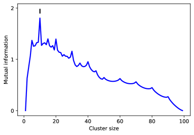
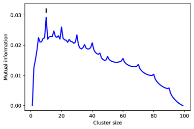
Figure 1 gives the similarity between clusterings $A^{(10)}$ and $A^{(s)}$ with respect to $s$ in terms of adjusted mutual information, for both notions of adjustment. We observe very close behaviors, suggesting that both notions of adjustment tend to capture the same patterns in the clusterings. Note that the maximum similarity is attained for $s=10$ in both cases, as expected. The similarity is equal to 0 for $s\in\{1,100\}$ for both cases, in agreement with Proposition 2. We also observe local peaks at $s=20,30,\ldots,90$, which can be interpreted by the fact that clustering $A^{(10)}$ is a refinement of clustering $A^{(s)}$ for these values of $s$; similarly, the local peak at $s=5$ may be interpreted by the fact that clustering $A^{(5)}$ is a refinement of clustering $A^{(10)}$.

(a) Full adjustment

(b) Pairwise adjustment

Figure 1: Comparison of metrics on synthetic data ($n=100$).

We now consider random clusterings. Specifically, we assign $n$ samples to $k$ clusters independently at random, according to some probability distribution $p=(p_{1},\ldots,p_{k})$, which is itself drawn at random. Consider three such random clusterings $A$, $B$, $C$ (with the same parameters $n$ and $k$, but different probability distributions $p$). We would like to know whether $A$ is “closer” to $B$ or to $C$. In particular, we are interested in testing whether both notions of adjusted mutual information give the same ordering in the sense that:

$$(s(A,B)-s(A,C))(s_{\rm p}(A,B)-s_{\rm p}(A,C))\geq 0.$$ (8)

We compute the average precision score (fraction of triplets $A,B,C$ for which (8) is true) over 1 000 independent samples of $A,B,C$, for different values of $n$ and $k$. We repeat the experiment 100 times to get the mean and standard deviation. The results are given in Table 1. We observe a very high precision score, always higher than $93\%$, showing that both notions of adjusted mutual information tend to give the same ordering of these random clusterings.

$n$	$k$	Precision score
100	2	$0.972\pm 0.004$
100	5	$0.952\pm 0.007$
100	10	$0.943\pm 0.006$
100	20	$0.955\pm 0.008$
500	20	$0.936\pm 0.007$
1000	20	$0.933\pm 0.006$
1000	50	$0.949\pm 0.008$

Table 1: Precision score (mean $\pm$ standard deviation)

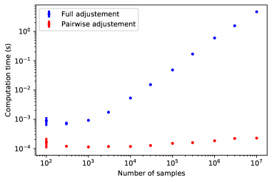
For the performance gain, we compare the computation times of both versions of adjusted mutual information for the similarity between clusterings $A$ and $B$, where $A$ consists of $k=10$ clusters of same size and $B$ is a random clustering, drawn as in the previous experiment. Both versions of adjusted mutual information are coded in Python, with the standard version imported from scikit-learn. Figure 2 shows the computation time when the number of samples $n$ grows from $10^{2}$ to $10^{7}$. The performance gain brought by pairwise adjustement is significant. In particular, the computation time becomes independent of the number of samples.

Figure 2: Computation time with respect to $n$ (mean $\pm$ standard deviation).

Real data.

For real data, we consider the 79 datasets of the benchmark suite [2]. We apply to each dataset each of the following clustering algorithms:

1. $k$-means

2. Affinity propagation

3. Mean shift

4. Spectral clustering

5. Ward

6. Agglomerative clustering

7. DBSCAN

8. OPTICS

9. Birch

10. Gaussian Mixture

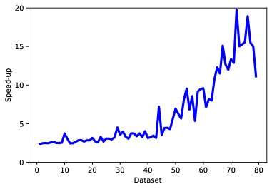
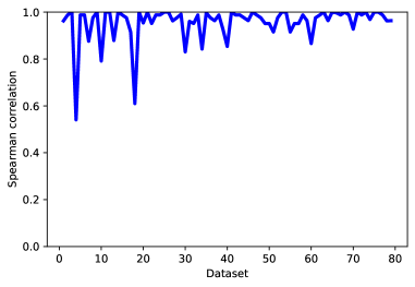
We use the scikit-learn implementation of these algorithms, with the corresponding default parameters. We get 10 clusterings per dataset. The quality of each clustering is assessed through the similarity with the available ground-truth labels, using adjusted mutual information with either full adjustment or pairwise adjustment. We then compute the Spearman correlation of the corresponding similarities, a value of 1 meaning the exact same ordering of the 10 clusterings with full adjustment and pairwise adjustment. The results are shown in Figure 3, together with the speed-up in computation time due to pairwise adjustment. In both cases, the 79 datasets are ordered by the number of samples, ranging from 105 to 105 600 [2].

(a) Spearman correlation.

(b) Speed-up of pairwise adjustment.

Figure 3: Comparison of metrics on real data.

We first observe that the correlation is very high, suggesting again that both notions of adjusted mutual information tend to provide the same results. For 65 datasets among 79, the Spearman correlation is higher than 95%. As for the computation time, we observe a significant performance gain, by one order of magnitude for the largest datasets.

6 Conclusion

We have proposed another way of adjusting mutual information against chance, through pairwise label permutations. The novel metric, whose explicit expression is given in Theorem 1, has a much lower complexity than the usual adjusted mutual information. Interestingly, both metrics can also be used to assess the quantity of information contained in a clustering, which the common property of being equal to 0 if and only if the clustering is trivial, as stated in Proposition 3; again, the pairwise adjusted entropy, given in Corollary 2, has a much lower complexity. Experiments on synthetic and real data show that pairwise adjusted mutual information tends to provide the same results as the usual adjusted mutual information for comparing clusterings, while involving much less computations.

For future work, we plan to extend this idea to other similarity metrics. While the practical interest is less obvious for the Adjusted Rand Index [3], due to the fact that the time complexity of this metric is already independent of the number of samples, it would be worth considering other versions of information theoretic measures, as those studied in [7].

Appendix

Proof of Proposition 1

The first equality follows from the fact that $X$ and $X_{\sigma}$ have the same distribution. Specifically, we have for any positive integer $k$,

$${\rm P}(X_{\sigma}=k) ={\rm P}((X\circ\sigma)^{-1}(k)),$$

$$={\rm P}(\sigma^{-1}(X^{-1}(k))),$$

$$={\rm P}(X^{-1}(k)),$$

$$={\rm P}(X=k).$$

For the second, we observe that if $\sigma$ is a random permutation of $\{1,\ldots,n\}$, chosen uniformly at random, so is $\sigma^{-1}$ which implies:

$${\rm E}(H(X,Y_{\sigma}))={\rm E}(H(X,Y_{\sigma^{-1}}))={\rm E}(H(X_{\sigma},Y)),$$

where we have used the first equality and the fact that:

$$(X,Y_{\sigma^{-1}})\circ\sigma=(X_{\sigma},Y).$$

The third equality is a direct consequence of the two first.

Proof of Proposition 2

If $Y$ is constant, then $Y=Y_{\sigma}$ for all permutations $\sigma$ and the result follows from (3). Now assume that $Y$ is a permutation of $\{1,\ldots,n\}$. Then $H(X,Y)=H(Y)=\log(n)$ and $I(X,Y)=H(X)$, for any random variable $X$. It then follows from (2) (and the symmetry in $X$ and $Y$) that

$$\Delta I(X,Y)=I(X,Y)-{\rm E}(I(X_{\sigma},Y))=0.$$

Proof of Proposition 3

If $\Delta H(X)=0$, then $d((X,X_{\sigma}))=0$ for all permutation $\sigma$. In particular, there exists some bijection $f$ such that $X_{\sigma}=f(X)$. Now assume that for some integer $i$, the event:

$$A=\{\omega:X(\omega)=i\}$$

is such that $1<|A| <n$. Then there exists some $j\neq i$ such that the event $B=\{\omega:X(\omega)=j\}$ is not empty. Choose $a\in A$ and $b\in B$ and define $\sigma$ as the permutation of $a$ and $b$. Then $X_{\sigma}(a)=X(b)=j$ while $X_{\sigma}(a^{\prime})=X(a^{\prime})=i$ for all $a^{\prime}\in A\setminus\{a\}$. So $X_{\sigma}(a)\neq X_{\sigma}(a^{\prime})$ while $X(a)=X(a^{\prime})$ for all $a^{\prime}\in A\setminus\{a\}$, which contradicts the existence of some mapping $f$ that $X_{\sigma}=f(X)$. Thus for each integer $i$, the cardinal of the event $A=\{\omega:X(\omega)=i\}$ is $0,1$ or $n$. This implies that $X$ is constant or equal to some permutation of $\{1,\ldots,n\}$.

Proof of Theorem 1

Consider two items selected uniformly at random in $\{1,\ldots,n\}$. Let $A_{i_{1}},B_{j_{1}}$ be the clusters of the first item, $A_{i_{2}},B_{j_{2}}$ be the clusters of the second item. In particular, these items belong respectively to the sets $A_{i_{1}}\cap B_{j_{1}}$ and $A_{i_{2}}\cap B_{j_{2}}$. The probability of this event is:

$$\frac{n_{i_{1}j_{1}}n_{i_{2}j_{2}}}{n^{2}}.$$

Now assume that these items exchange their labels for the first clustering, so that the first item move to set $A_{i_{2}}$ while the second item move to the set $A_{i_{1}}$. If $i_{1}=i_{2}$ or $j_{1}=j_{2}$, the new contingency matrix remains unchanged; now if $i_{1}\neq i_{2}$ and $j_{1}\neq j_{2}$, the new contingency matrix $n^{\prime}_{ij}$ remains unchanged except for the following entries:

$$n^{\prime}_{ij}=\left\{\begin{array}[]{ll}n_{ij}-1&\text{for }i,j=i_{1},j_{1}\text{ and }i_{2},j_{2},\\ n_{ij}+1&\text{for }i,j=i_{1},j_{2}\text{ and }i_{2},j_{1}.\end{array}\right.$$

Using (5), we obtain the similarity between clusterings $A$ and $B$:

$$s_{\rm p}(A,B) =\sum_{i_{1}\neq i_{2},j_{1}\neq j_{2}}\frac{n_{i_{1}j_{1}}n_{i_{2}j_{2}}}{n^{2}}$$

$$\times\left(\frac{n_{i_{1}j_{1}}}{n}\log\frac{n_{i_{1}j_{1}}}{n}-\frac{n_{i_{1}j_{1}}-1}{n}\log\frac{n_{i_{1}j_{1}}-1}{n}\right.$$

$$+\frac{n_{i_{2}j_{2}}}{n}\log\frac{n_{i_{2}j_{2}}}{n}-\frac{n_{i_{2}j_{2}}-1}{n}\log\frac{n_{i_{2}j_{2}}-1}{n}$$

$$+\frac{n_{i_{1}j_{2}}}{n}\log\frac{n_{i_{1}j_{2}}}{n}-\frac{n_{i_{1}j_{2}}+1}{n}\log\frac{n_{i_{1}j_{2}}+1}{n}$$

$$+\left.\frac{n_{i_{2}j_{1}}}{n}\log\frac{n_{i_{2}j_{1}}}{n}-\frac{n_{i_{2}j_{1}}+1}{n}\log\frac{n_{i_{2}j_{1}}+1}{n}\right),$$

where by convention, $x\log x=0$ for any $x\leq 0$. Observing that for any given $i_{1},j_{1}$,

$$\sum_{i_{2}\neq i_{1},j_{2}\neq j_{1}}n_{i_{1}j_{1}}n_{i_{2}j_{2}}=n_{i_{1}j_{1}}(n-a_{i_{1}}-b_{j_{1}}+n_{i_{1}j_{1}}),$$

while for any given $i_{1},j_{2}$,

$$\sum_{i_{2}\neq i_{1},j_{1}\neq j_{2}}n_{i_{1}j_{1}}n_{i_{2}j_{2}}=(a_{i_{1}}-n_{i_{1}j_{2}})(b_{j_{2}}-n_{i_{1}j_{2}}),$$

we get by symmetry:

$$s_{\rm p}(A,B) =2\sum_{i,j}\frac{n_{ij}(n-a_{i}-b_{j}+n_{ij})}{n^{2}}$$

$$\times\left(\frac{n_{ij}}{n}\log\frac{n_{ij}}{n}-\frac{n_{ij}-1}{n}\log\frac{n_{ij}-1}{n}\right)$$

$$+2\sum_{i,j}\frac{(a_{i}-n_{ij})(b_{j}-n_{ij})}{n^{2}}$$

$$\times\left(\frac{n_{ij}}{n}\log\frac{n_{ij}}{n}-\frac{n_{ij}+1}{n}\log\frac{n_{ij}+1}{n}\right).$$

Proof of Corollary 1

The proof follows on observing that the second sum in (7) can be written:

$$S \stackrel{{\scriptstyle d}}{{=}}\sum_{i,j}\frac{(a_{i}-n_{ij})(b_{j}-n_{ij})}{n^{2}}$$

$$\times\left(\frac{n_{ij}}{n}\log\frac{n_{ij}}{n}-\frac{n_{ij}+1}{n}\log\frac{n_{ij}+1}{n}\right)$$

$$=\sum_{i,j:n_{ij}>0}\frac{(a_{i}-n_{ij})(b_{j}-n_{ij})}{n^{2}}$$

$$\times\left(\frac{n_{ij}}{n}\log\frac{n_{ij}}{n}-\frac{n_{ij}+1}{n}\log\frac{n_{ij}+1}{n}\right)$$

$$-\sum_{i,j:n_{ij}=0}\frac{(a_{i}-n_{ij})(b_{j}-n_{ij})}{n^{2}}\frac{1}{n}\log\frac{1}{n}.$$

Since

$$\sum_{i,j:n_{ij}=0} {(a_{i}-n_{ij})(b_{j}-n_{ij})}=$$

$$\sum_{i,j}(a_{i}-n_{ij})(b_{j}-n_{ij})$$

$$-\sum_{i,j:n_{ij}>0}{(a_{i}-n_{ij})(b_{j}-n_{ij})}$$

$$=n^{2}-\sum_{i}a_{i}^{2}-\sum_{j}b_{j}^{2}$$

$$+\sum_{i,j}n_{ij}^{2}-\sum_{i,j:n_{ij}>0}{(a_{i}-n_{ij})(b_{j}-n_{ij})},$$

we get:

$$S =\sum_{i,j:n_{ij}>0}\frac{(a_{i}-n_{ij})(b_{j}-n_{ij})}{n^{2}}$$

$$\times\left(\frac{n_{ij}}{n}\log\frac{n_{ij}}{n}-\frac{n_{ij}+1}{n}\log\frac{n_{ij}+1}{n}+\frac{1}{n}\log\frac{1}{n}\right)$$

$$-\left(n^{2}-\sum_{i}a_{i}^{2}-\sum_{j}b_{j}^{2}+\sum_{i,j}n_{ij}^{2}\right)\frac{1}{n}\log\frac{1}{n}.$$

Proof of Corollary 2

The proof follows from (7) applied to the diagonal contingency matrix $n_{ij}=a_{i}\delta_{ij}=b_{j}\delta_{ij},$ where $\delta_{ij}$ denotes the Kronecker symbol.

References

• [1] T. M. Cover and J. A. Thomas. Elements of Information Theory. Wiley, 1991.
• [2] M. Gagolewski. Benchmark suite for clustering algorithms – version 1, 2020.
• [3] L. Hubert and P. Arabie. Comparing partitions. Journal of classification, 2(1):193–218, 1985.
• [4] M. Meilă. Comparing clusterings by the variation of information. In Learning theory and kernel machines, pages 173–187. Springer, 2003.
• [5] X. V. Nguyen, J. Epps, and J. Bailey. Information theoretic measures for clusterings comparison: is a correction for chance necessary? In ICML, 2009.
• [6] S. Romano, J. Bailey, V. Nguyen, and K. Verspoor. Standardized mutual information for clustering comparisons: one step further in adjustment for chance. In International Conference on Machine Learning, pages 1143–1151, 2014.
• [7] S. Romano, N. X. Vinh, J. Bailey, and K. Verspoor. Adjusting for chance clustering comparison measures. The Journal of Machine Learning Research, 17(1):4635–4666, 2016.
• [8] A. A. Taha and A. Hanbury. Metrics for evaluating 3d medical image segmentation: analysis, selection, and tool. BMC medical imaging, 15(1):29, 2015.
• [9] B. Thirion, G. Varoquaux, E. Dohmatob, and J.-B. Poline. Which fmri clustering gives good brain parcellations? Frontiers in neuroscience, 8:167, 2014.
• [10] N. X. Vinh, J. Epps, and J. Bailey. Information theoretic measures for clusterings comparison: Variants, properties, normalization and correction for chance. The Journal of Machine Learning Research, 11:2837–2854, 2010.
• [11] B. Wang, J. Zhu, E. Pierson, D. Ramazzotti, and S. Batzoglou. Visualization and analysis of single-cell rna-seq data by kernel-based similarity learning. Nature methods, 14(4):414–416, 2017.
• [12] Z. Yang, R. Algesheimer, and C. J. Tessone. A comparative analysis of community detection algorithms on artificial networks. Scientific reports, 6:30750, 2016.
• [13] J. Zhang, P. Kapli, P. Pavlidis, and A. Stamatakis. A general species delimitation method with applications to phylogenetic placements. Bioinformatics, 29(22):2869–2876, 2013.