Incrementally Zero-Shot Detection
by an Extreme Value Analyzer

Abstract

Human beings not only have the ability to recognize novel unseen classes, but also can incrementally incorporate the new classes to existing knowledge preserved. However, zero-shot learning models assume that all seen classes should be known beforehand, while incremental learning models cannot recognize unseen classes. This paper introduces a novel and challenging task of Incrementally Zero-Shot Detection (IZSD), a practical strategy for both zero-shot learning and class-incremental learning in real-world object detection. An innovative end-to-end model – IZSD-EVer was proposed to tackle this task that requires incrementally detecting new classes and detecting the classes that have never been seen. Specifically, we propose a novel extreme value analyzer to detect objects from old seen, new seen, and unseen classes, simultaneously. Additionally and technically, we propose two innovative losses, i.e., background-foreground mean squared error loss alleviating the extreme imbalance of the background and foreground of images, and projection distance loss aligning the visual space and semantic spaces of old seen classes. Experiments demonstrate the efficacy of our model in detecting objects from both the seen and unseen classes, outperforming the alternative models on Pascal VOC and MSCOCO datasets.

I Introduction

This paper studies object detection, which, as one important computer vision task, has seen unprecedented advances in recent years with the development of Convolutional Neural Network (CNN). However, most successful object detection models, to data, are formulated as supervised learning problems in a batch setting. Such detection models have limited the capability of generalizing to unseen object classes, or being learned in an incremental setting. Humans, on the other hand, not only have the ability to recognize novel unseen object classes, but incrementally incorporate these novel object classes to existing knowledge preserved as well. For instance, a boy visiting the zoo will continuously identify and remember many new animals whilst not forget his pet at home.

Previous endeavors tackle object detection in either zero-shot learning (ZSL) [1], or class-incremental manner [2, 3]. Particularly, model learns to recognize and localize objects from unseen classes in Zero-Shot Detection (ZSD) [1, 4, 5, 6, 7]. A successful ZSL model should have effective semantic knowledge transfer, i.e., transferring knowledge of seen classes, such as semantic attributes or word vector, to unseen classes. However, the ZSL assumes that all seen classes should be known beforehand, and the recognition model is trained in a batch; this greatly and unrealistically simplified the problem in the real-world setting. In contrast, the class-incremental learning (CIL) task  [8, 9, 10] aims at continuously learning newly observed classes without forgetting existing old classes, i.e., catastrophic forgetting [11]. The CIL model is trained via a stream of data in which examples of different classes occur at different times. Notably, without semantic knowledge transfer as ZSL, CIL classifiers are not capable of inferring of objects of unseen classes in testing.

Critically, it would be desirable for vision systems to be able to perform incrementally zero-shot detection (IZSD). Particularly, referring to the properties of CIL in iCaRL [9], we quantify several properties of an algorithm qualified as IZSD: (1) an object detection model is trained from a stream of data, in which visual examples and semantic information of different object classes are observed at different incremental steps; (2) the model, at current incremental step, should not be updated by examples, from existing (old seen) object classes, but only from newly observed (new seen) object classes, which are unseen classes in previous incremental steps, as illustrated in Fig. 1. (3) The trained model should at any time provide a competitive detector for new seen, old seen and unseen object classes, (4) by the bounded, memory footprint, and computational cost, with respect to the number of seen object classes at each incremental step.

These criteria, essentially, identifies the key difference between IZSD and CIL/ZSL, as well as excluding the trivial solutions in memorizing all seen objects to retrain a zero-shot detector at each incremental step (the Fourth Criterion). Specifically, the IZSD should, in principle, maintain an updated incremental object detector by leveraging both visual and semantic representations of new seen object classes at each incremental step. In contrast, the naive solutions by either visual or semantic cues may be tempted to the deteriorated detection results. For example, one can directly incrementally update ZSD models by using the semantic information from new seen object classes. However, the predictions of such models may be biased towards the old seen object classes, as the corresponding visual feature extractor is not updated by the visual information from these new seen object classes. On the other hand, the typical class-incremental object detector [2, 3], updated by the visual cues (but not semantics) of new seen object classes, is not capable of localizing objects from those classes that are unseen at the current incremental step. These two naive baselines are compared in Tab. VI.

A good IZSD model should be both efficient in semantic knowledge transfer, and robust to catastrophic forgetting. However, at one incremental step, the model may be prone to overfitting new seen classes, as they are blind to semantic embeddings of unseen object classes [12], and catastrophically forget the visual representations of old seen classes. Towards this technical difficulty of IZSD, we propose a novel extreme value analyzer (EVer), in differentiating the unseen, from both new and old seen classes by comparing the extreme values [13] of each class in the semantic spaces. Furthermore, derived from knowledge distillation, a novel old-new model is presented to help remember both the visual and semantic information of old seen classes.

Formally, we propose a novel end-to-end object detection model for IZSD by EVer (IZSD-EVer), with the key components of the old-new model and EVer. Specifically, with the backbone of Faster RCNN (FRCN) [14], the old-new model maintains the visual and semantic knowledge of old seen classes, by knowledge distillation [15] and projection distance loss, with a memory component introduced. Furthermore, inspired by Extreme Value Theory (EVT) [13], EVer, in the semantic space, measures the similarity of each instance to the mean vectors of instances from each seen class by generalized Pareto distribution (GPD) [16]. EVer, in the testing, infers the GPD probability of belonging to seen or unseen classes, one sample which is further predicted by either the incremental classifier or zero-shot classifiers. On the benchmark dataset, we extensively evaluate IZSD-EVer, and the results demonstrate the efficacy of IZSD-EVer in solving the IZSD task.

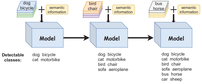
Figure 1: Incrementally zero-shot detection. At each incremental step, examples of new seen object classes and semantic information are utilized to update the detection model. The model is able to detect objects from old seen, new seen, and unseen classes. If there is only one incremental step, then IZSD is equivalent to zero-shot detection. In addition, if semantic information is not utilized to detect unseen object classes, the model is equivalent to perform class-incremental detection.

We make four main contributions in this paper: (1) We introduce a new object detection task of incremental zero-shot detection, a practical strategy for both ZSL and CIL in the real-world object detection. (2) We propose an innovative end-to-end trainable model – IZSD-EVer in addressing IZSD by integrating ZSL and CIL in a single framework. (3) A novel extreme value analyzer, is presented, to simultaneously detect objects from old seen, new seen, and unseen classes. To the best of our knowledge, the GPD in EVT, is for the first time, introduced for both object detection and class-incremental learning. (4) Additionally and technically, we propose two novel losses, i.e., backgroud-forground mean squared error (bfMSE) alleviating the extreme imbalance of the background and foreground of images, and projection distance (PD) loss aligning the visual and semantic spaces of old seen classes.

II Related Works

Zero-Shot Detection The task of ZSL is seeking to recognize unseen visual categories [17, 18, 19, 20, 21, 22]. As an extension, ZSD aims at recognizing and localizing the objects of unseen classes in testing [5, 1, 4, 23, 6, 7]. Specifically, they adapt the existing detectors (2-stage for [5, 1, 6, 7], 1-stage for [4, 23]) in the ZSD setting by adding a separate semantic prediction training task on the annotated seen objects, such that domain knowledge can be transferred to detect unseen objects which are semantically similar to seen objects. Among them, Rahman et al. [6] proposed polarity loss explicitly maximizing the margin between predictions for positive and negative classes based on focal loss. In contrast, our IZSD-EVer employs the proposed bgMSE loss as well as reconstruction loss and triplet loss. Generally, the ZSL assumes the model trained in a batch, whilst the proposed IZSD task requires model learning in a class-incremental manner, which is more realistic in real-world applications.

Class-Incremental Detection Researchers have proposed many different approaches to solve class-incremental learning [10, 8, 9, 24, 25, 26]. However, these methods focus on solving image classification task rather than more difficult object detection task. Class-incremental detection aims at adding new classes to well-trained object detector incrementally, using only the data of the new classes, independent with totally re-training. Shmelkov et al. [2] presented the first approach to solve the task of class-incremental detection, by a two-stage object detection model on Fast R-CNN [27] with proposals generated by EdgeBoxes [28]. The model alleviates catastrophic forgetting by optimizing cross-entropy loss and knowledge distillation loss [15]. However, this model is not an end-to-end model and requires the external EdgeBoxes to generate proposals, which consume many computing resources. In contrast, Hao et al. [3] proposed an end-to-end architecture for class incremental detection. Based on FRCN, they introduced knowledge distillation in both Region Proposal Network (RPN) and FRCN, transferring knowledge from teacher subnetwork to student subnetwork to generate high-quality box proposals, preventing catastrophic forgetting. Again, object detection in this setting, is different from our IZSD, as their incapable of predicting objects from unseen classes, and functionally, our EVer is proposed for such a purpose, inspired by recent works on open set recognition by extreme values in computer vision [29, 30, 31, 32, 33].

III Proposed Model

Problem Setup. In an incremental step, a set of old seen classes denoted as $\mathcal{O}$, whose samples have been used to train the model in the previous incremental steps. Moreover, a set of new seen classes $\mathcal{N}$, whose samples are training data of the current incremental step. There is also a set of unseen classes $\mathcal{U}$, whose samples are only accessible during the test phase. These three sets of classes are mutually exclusive, i.e., $\mathcal{O}\cap\mathcal{N}\cap\mathcal{U}=\varnothing$, so the set of all classes is denoted by $\mathcal{C}=\mathcal{O}\cup\mathcal{N}\cup\mathcal{U}$. The set of seen classes is $\mathcal{S}=\mathcal{O}\cup\mathcal{N}$. Besides, $N_{\mathcal{O}}$, $N_{\mathcal{N}}$, $N_{\mathcal{U}}$, $N_{\mathcal{S}}$, $N_{\mathcal{C}}$ represent the number of old seen, new seen, unseen, all seen, and all classes, respectively. We denote semantic information as $\mathbf{E}\in\mathbb{R}^{(C+1)\times d}$ composed of $(C+1)$ semantic embeddings (e.g., word2vec [34], GloVe [35], attributes) of $d$ dimensions as its rows. Each object class has a corresponding semantic embedding, including the background class. The semantic embedding of the background class is the mean semantic embedding of other classes, i.e., $\mathbf{E}_{0,:}=\frac{1}{C}\sum_{i=1}^{C}\mathbf{E}_{i,:}$, which is the same as [1]. Given a model well-trained on old classes dataset $\mathcal{X_{O}}$, the IZSD model is updated by new classes dataset $\mathcal{X_{N}}$ at current incremental step, and is capable of generalizing to predict examples from $\mathcal{O}$, $\mathcal{N}$ and $\mathcal{U}$, individually. Additionally, we introduce a bounded memory $\mathcal{M}=\{x_{i},i=1,2,\dots,K\}$, with memory size $K$ is much smaller than the number of $\mathcal{X_{O}}$, i.e., ${K}\ll N_{\mathcal{O}}$.

End-to-End Learning of IZSD-Ever. The model is learned in an end-to-end way. In the first incremental step, since no existing old classes, the new model performs end-to-end learning on $\mathcal{X_{N}}$ through the following loss function.

$$\mathcal{L}=\mathcal{L}_{bone}+\mathcal{L}_{cls}.$$ (1)

Then we estimate the parameters of GPD by maximum likelihood estimation (MLE) based on the projected semantic vectors for each new class. We store the most representative images for each new class in the memory component, as described in Sec. III-B. In the subsequent incremental steps, the new class dataset $\mathcal{X_{N}}$ and memory $\mathcal{M}$ are simultaneously inputted into the old and new models, and the new model is trained end-to-end using the following loss function.

$$\mathcal{L}=\mathcal{L}_{bone}+\mathcal{L}_{IL}.$$ (2)

For the new classes, we estimate the parameters of the GPD for them as in the first incremental step. The parameters of GPD of the old classes remain unchanged. The memory $\mathcal{M}$ is also updated accordingly. We will introduce each loss in the following subsection.

III-A Backbone with Semantic Embedding

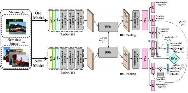
Figure 2: The overall architecture of our IZSD-EVer model.

Built upon the backbone of FRCN, we additionally add the semantic embedding. Particularly, as shown in Fig. 2, we denote the visual feature of the fully connected (FC) layer before zero-shot classifier as $f(x;\Theta)\in\mathbb{R}^{v}$, where $x$ and $\Theta$ denote the input image, the weights of FRCN model, individually. It is followed by another FC layer for zero-shot classifier, projecting visual features from visual space to $d$-dimensional semantic space denoted by $\mathbf{W}\in\mathbb{R}^{d\times v}$, as $\mathbf{s}=\mathbf{W}f(x;\Theta),\quad\mathbf{s}\in\mathbb{R}^{d}$. Cosine similarity is employed to measure the distance between projected semantic vector $\mathbf{s}$ and semantic embedding of classes $\mathbf{E}$, and output the predicted class probability, as $\mathbf{p}^{zsc}=\mathtt{softmax}(\mathbf{Es}),\quad\mathbf{p}^{zsc}\in\mathbb{R}^{N_{\mathcal{C}}+1}$, where $\mathbf{s}$ and $\mathbf{E}$ are $\ell^{2}$ normalized.

To efficiently learn the trainable $\mathbf{W}$, we present three loss functions to help align visual features and with corresponding semantic embeddings. Particularly,

bfMSE Loss. We train $\mathbf{W}$ using background-foreground MSE (bfMSE) loss to alleviate extreme imbalance between background and foreground in proposals generated by RPN. We separately compute MSE loss between the projected semantic vectors of background and foreground and the corresponding semantic embeddings. The bfMSE loss is defined as

$$\mathcal{L}_{bfmse} =\frac{1}{N_{bg}}\sum_{i=1}^{N_{bg}}\mathbb{I}_{i}^{bg}\|\mathbf{s}_{i}-\mathbf{E}_{0,:}\|_{2}^{2}$$ (3)

$$+\alpha\frac{1}{N_{obj}}\sum_{i=1}^{N_{obj}}\mathbb{I}_{i}^{obj}\|\mathbf{s}_{i}-\mathbf{E}_{y_{i},:}\|_{2}^{2},$$

where $\mathbb{I}_{i}^{bg}$ and $\mathbb{I}_{i}^{obj}$ are indicators showing that the $i$-th region proposal contains background and object, respectively. $N_{bg}$ and $N_{obj}$ are the number of region proposals belonging to the background and foreground, respectively. $y_{i}$ is the ground-truth label of $i$-th region proposal. We empirically set $\alpha=5$.

Reconstruction Loss. We introduce this loss in [36] to learn a more generalized model, as

$$\mathcal{L}_{rec}=\frac{1}{N_{p}}\sum_{i=1}^{N_{p}}\|f(x;\Theta)-\mathbf{W}^{T}\mathbf{s}\|_{2}^{2},$$ (4)

where $\mathbf{W}^{T}$ project $\mathbf{s}$ back to visual space to reconstruct the visual feature. $N_{p}=N_{bg}+N_{obj}$ is the number of proposals. Then we compute the MSE loss between the reconstructed visual features and the original visual features. Note that $\mathcal{L}_{bfmse}$ and $\mathcal{L}_{rec}$ are to constrain the projected semantic vectors to be similar to semantic embedding.

Triplet Loss. This loss enforces the projected semantic vectors are more similar semantic embedding of ground-truth classes, than those from other classes, defined as

$$\mathcal{L}_{tri}=\frac{1}{N_{p}}\sum_{i=1}^{N_{p}}\sum_{\begin{subarray}{c}j=1\\ j\neq y_{i}\end{subarray}}^{N_{\mathcal{S}}}\max(m+C_{ij}-C_{iy_{i}},0),$$ (5)

where $C_{ij}$ is the cosine similarity between the $\mathbf{s}_{i}$ and $\mathbf{E}_{j,:}$. Similarly, $C_{iy_{i}}$ is the cosine similarity between the $\mathbf{s}_{i}$ and its ground-truth semantic embedding $\mathbf{E}_{y_{i},:}$. In addition, the standard losses in FRCN are also utilized here as $\mathcal{L}_{FRCN}=\mathcal{L}_{cls}^{rpn}+\mathcal{L}_{reg}^{rpn}+\mathcal{L}_{reg}$, where $\mathcal{L}_{rpn}^{cls}$, $\mathcal{L}_{rpn}^{reg}$ and $\mathcal{L}_{reg}$ are the classification loss in RPN, bounding box regression loss in RPN and bounding box regression loss of bounding box regressor, respectively.

$$\mathcal{L}_{FRCN}=\mathcal{L}_{cls}^{rpn}+\mathcal{L}_{reg}^{rpn}+\mathcal{L}_{reg}$$ (6)

The overall loss function of the backbone model is

$$\mathcal{L}_{bone} =\mathcal{L}_{FRCN}+\mathcal{L}_{bfmse}+\beta\mathcal{L}_{rec}+\mathcal{L}_{tri},$$ (7)

where $\beta$ is a hyperparameter to control the importance of different losses.

III-B The Old-New Model

The bounded memory component $\mathcal{M}$ [24, 26, 25, 9] is introduced into our old-new model to alleviate the imbalance between old seen and new seen classes. Particularly, $\mathcal{M}$ stores a few images for each seen classes based on their representative object example visual features $f(x;\Theta)$, which closest to the mean feature vector of the classes. Since $\mathcal{M}$ has a limited memory capacity of $K$, it will clear the least representative images of each class as new seen classes come.

The old-new model is presented to incrementally learn new seen classes without catastrophic forgetting old seen classes. Specifically, as in Fig. 2, we add an incremental classifier to the backbone model. When new seen classes $\mathcal{N}$ occurs at the current incremental step, we combine the old model learned in previous steps, with the new model learned in this step, forming the old-new model. When incremental learning is performed, new class dataset $\mathcal{X}_{\mathcal{N}}$ and memory $\mathcal{M}$ are simultaneously entered into the old-new model, where the parameters of the old model are fixed. When our old-new model learns new classes, the RPN of the new model needs to be able to generate region proposals containing objects of the old or new classes. We re-purpose the domain expansion in RPN of [3] to maintain the knowledge of the old class. Thus, we freeze the RPN classifier to keep the decision boundary of the RPN classifier unchanged and update the parameters of other parts of the RPN, making the feature distance loss.

$$\mathcal{L}_{fd}^{rpn}=\|f_{rpn}(x;\Theta_{o})-f_{rpn}(x;\Theta_{n})\|_{F}^{2}.$$ (8)

$f_{rpn}(\cdot)$ denotes the feature map generated by the intermediate convolutional layer of RPN. This loss ensures that the RPN generates proposals containing objects of new or old classes.

When learning with new classes, the number of output nodes of the incremental classifier in the new model is expanded to the number of classes that have seen. As shown in Fig. 3, besides the traditional cross-entropy loss on all classes, we add a knowledge distillation loss [15] on the incremental classifier to transfer knowledge from the old model to the new model to alleviate performance dropping on old seen classes. Besides, we also add a projection distance (PD) loss on the zero-shot classifier to maintain the ability to align the visual space and semantic spaces of old seen classes. Particularly, let us denote the projected semantic embeddings of the old and new models as $\mathbf{s}_{o}$ and $\mathbf{s}_{n}$, respectively. Similarly, we denote the output logits of the incremental classifier as $\hat{y}_{o}$ and $\hat{y}_{n}$ for the old and new models, respectively.

$$\mathcal{L}_{cls}^{distill} =\mathtt{CE}(\mathtt{softmax}(\frac{\hat{y}_{o}}{T}),\mathtt{softmax}(\frac{\hat{y}_{n}^{o}}{T})),$$ (9)

$$\mathcal{L}_{cls} =\mathtt{CE}(y,\mathtt{softmax}(\hat{y}_{n})),$$ (10)

$$\mathcal{L}_{pd}^{zsc} =\|\mathbf{s}_{o}-\mathbf{s}_{n}\|_{2}^{2},$$ (11)

where $\hat{y}_{n}^{o}$ is the output logits of the new model for old classes. $y$ is the ground-truth label. $T$ is a temperature scalar. $\mathtt{CE}(\cdot)$ represents the cross-entropy loss. The overall loss function for incremental learning as follows:

$$\mathcal{L}_{IL}=\frac{N_{\mathcal{O}}}{N_{\mathcal{C}}}\left(\mathcal{L}_{cls}^{distill}+\mathcal{L}_{pd}^{zsc}\right)+\frac{N_{\mathcal{N}}}{N_{\mathcal{C}}}\mathcal{L}_{cls}+\gamma\mathcal{L}_{fd}^{rpn}.$$ (12)

The first three items are multiplied by the ratio of the class they are responsible for, indicating their importance during training. It reduces the hyperparameters and makes the model easier to train. And $\gamma$ is a hyperparameter.

III-C Extreme Value Analyzer

We construct an EVer as the Pickands-Balkema-de Haan Theorem [37] to differentiate unseen from seen object classes. Typically, let $X_{1},X_{2},\dots,X_{n}$ be a sequence of identically distributed random variables (i.i.d) with cumulative distribution function $F$. The conditional excess distribution function of $X$ over a threshold $u$ is defined as

$$F_{u}(x)=\Pr(X-u\leqslant x|X>u)=\frac{F(x+u)-F(u)}{1-F(u)},x\geqslant 0.$$ (13)

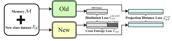
Figure 3: Diagram of incremental learning for IZSD.

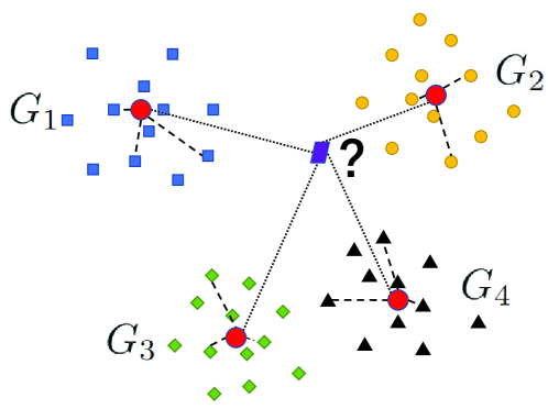
Figure 4: Extreme Value Analyzer. $G_{1},G_{2},G_{3},G_{4}$ represent the fitted GPD.

Theorem III.1 (Pickands–Balkema–de Haan theorem)

[37] The conditional excess distribution function $F_{u}$ can be well approximated by the generalized Pareto distribution when the threshold $u$ is sufficiently large. That is

$$F_{u}(x)\to G(x;\sigma,\xi),\quad\text{as}~{}u\to\infty$$ (14)

The GPD is defined as

$$G(x;\sigma,\xi)=\left\{\begin{array}[]{ll}1-\left(1+\xi\frac{x}{\sigma}\right)^{-\frac{1}{\xi}},&\xi\neq 0,\\ 1-\exp\left(-\frac{x}{\sigma}\right),&\xi=0,\end{array}\right.$$ (15)

$x\geqslant\mu$ when $\xi\geqslant 0$, $\mu\leqslant x\leqslant\mu-\frac{1}{\xi}$ when $\xi<0$.

In the semantic space, the projected semantic vectors of the same class are close together, and the projected semantic vectors of the different classes are far away from each other. As shown in Fig. 4, we propose to use the GPD of EVT to model the projected semantic vectors for each seen class. Particularly, if the distance between one projected semantic vectors to the mean projected semantic vector exceeds a threshold, such projected semantic vector would be taken as an extreme semantic vector. To this end, we fit the GPD based on the distance beyond the threshold.

We first compute the Euclidean distance $d_{ij}$ between the projected semantic vectors $\mathbf{s}_{j}^{i}$ and the mean projected semantic vector $\overline{\mathbf{s}}_{j}$ of $j$-th class, i.e., $d_{ij}=\|\mathbf{s}_{j}^{i}-\overline{\mathbf{s}}_{j}\|_{2},j\in\{1,2,\dots,S\}$, where $\mathbf{s}_{j}^{i}$ and $\overline{\mathbf{s}}_{j}$ are $\ell^{2}$ normalized. Then we get the estimated parameters $\hat{\sigma}_{j}$ and $\hat{\xi}_{j}$ of GPD by MLE based on the excess of distance exceeding threshold $u_{j}$ for $j$-th class. In classifying, we compute the excess of distance $\|\mathbf{s}-\overline{\mathbf{s}}_{j}\|_{2}$ beyond threshold $u_{j}$, and then derive the probability that the semantic vector is an extreme semantic vector by substituting the excess into the GPD, that is, the probability of not belonging to the $j$-th class. We get $P_{min}$ over seen classes as follows.

$$P_{min}=\min_{j\in\{1,2,\dots,S\}}G(\|\mathbf{s}-\overline{\mathbf{s}}_{j}\|_{2}-u_{j},\hat{\sigma}_{j},\hat{\xi}_{j}).$$ (16)

We obtain the prediction class label for the region proposal by the following

$$\hat{y}=\left\{\begin{array}[]{ll}\mathop{\arg\max}_{i\in\{1,2,\dots,S\}}\mathbf{p}_{i}^{ic},&P_{min}<\delta,\\ \mathop{\arg\max}_{i\in\{1,2,\dots,U\}}\mathbf{p}_{i}^{zsc},&P_{min}\geqslant\delta,\end{array}\right.$$ (17)

where $\delta$ is a threshold. If $P_{min}\geqslant\delta$, then $\mathbf{s}$ is an extreme semantic vector for all seen classes, the corresponding region proposal belongs to unseen classes. Conversely, if $P_{min}<\delta$, the corresponding region proposal belongs to seen classes.

IV Experiments

IV-A Datasets and Settings

Dataset: We evaluate our model on Pascal VOC 2007 and 2012 datasets [38] and MSCOCO 2014 and 2017 datasets [39], respectively. MSCOCO is a large-scale dataset for object detection, segmentation, and captioning. This dataset is more challenging than Pascal VOC as it has 80 object classes, more small objects, and more complex background. Our model is compared in CIL and ZSL settings. Specifically, for class-incremental detection, we use the same datasets VOC 2007 and MSCOCO 2017 as [3, 2]. For zero-shot detection, we use VOC 2007 and MSCOCO 2014 as [23, 6]. In order to compare fairly with other ZSD methods, we use the train split of VOC 2007 and 2012 (with 20 object classes) during training and use val+test split of VOC 2007 for testing.

Evaluation Metric: We use the standard average precision (AP) at 0.5 IoU threshold over each class, and mean average precision (mAP) over all the classes as the evaluation metric.

TABLE I: Old classes, new class and unseen classes split in different incremental step.

Step	Old classes	New classes	Unseen classes	Train data	Test data
1	-	$\mathcal{G}_{1}$	$\mathcal{G}_{2},\mathcal{G}_{3},\mathcal{G}_{4}$	$\mathcal{D}_{tr}(\mathcal{G}_{1})$	$\mathcal{D}_{te}(\mathcal{C})$
2	$\mathcal{G}_{1}$	$\mathcal{G}_{2}$	$\mathcal{G}_{3},\mathcal{G}_{4}$	$\mathcal{D}_{tr}(\mathcal{G}_{2})$
3	$\mathcal{G}_{1},\mathcal{G}_{2}$	$\mathcal{G}_{3}$	$\mathcal{G}_{4}$	$\mathcal{D}_{tr}(\mathcal{G}_{3})$
4	$\mathcal{G}_{1},\mathcal{G}_{2},\mathcal{G}_{3}$	$\mathcal{G}_{4}$	-	$\mathcal{D}_{tr}(\mathcal{G}_{4})$

TABLE II: The detail results of IZSD-EVer on VOC 2007

Step	aero- plane	bicycle	bird	boat	bottle	bus	car	cat	chair	cow	dining table	dog	horse	motro- bike	person	potted plant	sheep	sofa	train	tvmo- nitor	Seen	Unseen	mAP
1	57.2	72.8	31.7	41.3	24.3	0.9	6.9	0.2	0.0	0.3	0.0	0.3	0.3	26.3	0.4	0.0	1.0	0.0	9.5	0.1	45.5	3.1	13.7
2	50.3	61.3	51.3	29.8	22.2	54.0	74.9	73.6	23.1	41.5	0.1	9.1	5.8	16.8	0.8	0.1	1.1	13.9	10.9	0.2	48.2	5.9	27.0
3	51.2	54.4	51.2	31.0	26.4	45.3	72.7	66.2	22.2	37.4	62.3	64.4	73.2	69.7	67.2	0.0	3.2	12.1	12.6	0.1	53.0	5.6	41.1
4	59.1	67.0	61.3	39.8	36.7	51.9	74.9	68.4	19.8	38.8	41.9	58.7	71.7	73.5	69.6	29.3	60.8	67.4	72.5	59.2	56.1	-	56.1

TABLE III: The results of class-incremental detection on VOC 2007 and COCO 2017. Gray region means that the results of these groups can only be predicted in our model

Dataset	Method	$\mathcal{G}_{1}$	$\mathcal{G}_{2}$	$\mathcal{G}_{3}$	$\mathcal{G}_{4}$	mAP	Method	$\mathcal{G}_{1}$	$\mathcal{G}_{2}$	$\mathcal{G}_{3}$	$\mathcal{G}_{4}$	mAP	Method	$\mathcal{G}_{1}$	$\mathcal{G}_{2}$	$\mathcal{G}_{3}$	$\mathcal{G}_{4}$	mAP
		61.9	-	-	-	61.9		63.9	-	-	-	63.9		66.3	-	-	-	66.3
		33.3	67.8	-	-	50.6		43.8	71.2	-	-	57.5		44.8	59.2	-	-	52.0
		13.5	23.1	55.8	-	30.8		35.3	49.0	68.4	-	50.9		49.0	43.4	48.6	-	47.0
	Faster RCNN (Fine- tuning)	14.2	21.5	44.0	52.5	33.1	CIFRCN	34.6	44.1	55.6	59.6	48.5	IDWCF	40.2	35.5	42.5	38.8	39.3
		64.0	-	-	-	64.0		56.8	-	-	-	56.8		45.5	1.7	5.5	2.1	13.7
		65.2	73.2	-	-	69.2		40.4	68.8	-	-	54.6		43.0	53.4	6.5	5.2	27.0
		66.2	71.3	77.3	-	71.6		38.5	50.9	69.5	-	53.0		42.8	48.8	67.4	5.6	41.1
VOC 2007	Faster RCNN (Retrain)	65.1	70.4	76.4	67.8	69.9	CIFRCN NP	33.7	44.6	56.8	51.8	46.7	Ours	52.8	50.7	63.1	57.9	56.1
		58.3	-	-	-	58.3		58.1	-	-	-	58.1		49.2	-	-	-	49.2
		33.5	21.0	-	-	27.3		39.0	24.6	-	-	31.8		44.7	15.7	-	-	30.2
		20.1	11.9	26.4	-	19.5		29.9	18.5	29.6	-	26.0		42.4	13.1	14.0	-	23.2
	Faster RCNN (Fine- tuning)	16.8	9.3	9.4	31.4	16.7	CIFRCN	29.0	14.5	14.6	33.3	22.9	IDWCF	38.0	12.6	11.9	21.0	20.9
		58.4	-	-	-	58.4		55.6	-	-	-	55.6		46.5	2.9	0.1	0.2	12.4
		56.1	27.4	-	-	41.8		38.3	24.1	-	-	31.2		18.8	16.9	0.1	0.2	9.0
		54.9	26.6	30.8	-	37.4		26.2	18.6	27.2	-	24.0		10.8	10.1	20.3	0.1	10.3
COCO 2017	Faster RCNN (Retrain)	54.8	26.3	28.0	37.2	36.6	CIFRCN NP	26.5	15.1	15.5	32.2	22.3	Ours	38.4	15.9	12.3	26.9	23.4

Classes Split: For class-incremental detection, we follow the classes split as [3]. As shown in Tab. X, we split all classes into four class groups denoted by $\mathcal{G}_{1}$, $\mathcal{G}_{2}$, $\mathcal{G}_{3}$ and $\mathcal{G}_{4}$. Specifically, we sort all 20 classes of VOC 2007 alphabetically, split them into four class groups equally, so that each class group contains five classes. We remove images that contain objects from two or more class groups. As shown in Tab. X, we use $\mathcal{D}_{tr}(\cdot)$ and $\mathcal{D}_{te}(\cdot)$ to represent training and testing data that only contain objects of classes within the corresponding class group, respectively. For MSCOCO 2017, we use the same split method as for VOC 2007, except that the class order in MSCOCO 2017 is specified by itself. For the seen/unseen classes split for ZSD, we follow the split for VOC 2007 and 2012 proposed by [23]. Particularly, car, dog, soft, and train as unseen classes, other classes as seen classes. There are two different types of seen and unseen classes splits setting for MSCOCO 2014: the 48/17 and 65/15 seen/unseen classes splits proposed by [5] and [6], respectively.

TABLE IV: Results of ZSD on COCO 2014 by 48/17 and 65/15 seen/unseen classes split

Method	Seen/Unseen classes split	Unseen
PLZSD	48/17	10.01
Ours	48/17	15.29
PLZSD	65/15	12.40
Ours	65/15	20.67

Semantic Embedding: Many ZSD models use manual attributes and unsupervised word2vec/GloVe as semantic embeddings [1, 4, 40]. aPascal-aYahoo dataset [41] has 64-dimensional binary attributes that characterize the visible objects for 20 object classes of Pascal VOC [40]. Therefore, we use the 64-dimensional attributes of aPascal-aYahoo dataset for Pascal VOC in our experiments. Inspired by [6], we use the $l_{2}$ normalized 300-dimensional unsupervised word2vec[34] trained on billions of words from texts like Wikipedia for MSCOCO in our experiments.

TABLE V: The result of ZSD on Pascal VOC 2007 val+test split

Method	car	dog	sofa	train	mAP
HRM	55.0	82.0	55.0	26.0	54.5
PLZSD	63.7	87.2	53.2	44.1	62.1
Ours	47.26	89.3	57.0	41.4	58.7

Implementation: We use Faster RCNN as the backbone. As in Fig. 2, we use ResNet-101 as feature extractor that initialized by the weights pre-trained on ImageNet. Then we add one FC layer for Pascal VOC and three FC layers for MSCOCO followed by three branches predicting class probability for seen and unseen classes and bounding box coordinates. We empirically set $\alpha=5$ in Eq. 3, margin $m=1$ in Eq. 5 and $\beta=0.001$ in Eq. 7. $T$ in Eq. III-B is set to 2 following the suggestion in [15]. In addition, we set $\gamma=2$ in Eq. 12 like [3]. To set an appropriate threshold $u_{j}$ of GPD for $j$-th class, we sort $d_{ij}$ in the descending order, then set $u_{j}=\eta len(d_{ij}),\eta=0.2$, where $len(\cdot)$ is the length of $d_{ij}$. We choose it as 80% higher order quantile of the distances. We set $\delta=0.02$ in Eq. 17 by grid search. We set the memory size $K=150$ and $K=600$ for Pascal VOC and MSCOCO, respectively. Our model is trained by 10 epochs for each incremental step with batch sizes of 3 images per GPU. We set the learning rate by 0.001 at the beginning of each incremental step, and decrease it by 0.2 after 5 epochs.

IV-B Results on Incrementally Zero-Shot Detection

We rigorously evaluate our IZSD-Ever on both VOC 2007 and COCO 2017 datasets. We train our model by incrementally adding new classes and semantic information. As shown in Tab. X, in the first incremental step, we train the model on $\mathcal{D}_{tr}(\mathcal{G}_{1})$ containing class group $\mathcal{G}_{1}$, and in the subsequent incremental steps, new classes are added continuously and trained using the corresponding train data. Tab. II and Tab. III present the results on IZSD of our IZSD-Ever. As shown in Tab. II, our model not only can keep the knowledge of the old class well, but also can effectively detect unseen classes. However, the performance of unseen classes is lower than that of seen classes, which is caused by the inherent domain drift problem [40] of ZSL. It refers to the difference in the data distribution of seen classes and unseen classes, which leads to performance degradation in unseen classes. We have also observed that some unseen classes perform poorly. This is because the unseen class needs to be semantically similar to some seen classes to effectively transfer knowledge from the seen classes to the unseen classes recognition task. Therefore, a good seen/unseen classes split can improve performance on unseen classes, as described in seen/unseen classes split in classes split III. In addition, in Tab. III, the performance of our model in COCO2017 is relatively worse than that in VOC2007. On the one hand, it is because COCO is more challenging than VOC2007. On the other hand, compared with seen/unseen classes split of MSCOCO, too many unseen classes result in poor performance on unseen classes.

IV-C Results on Class-Incremental Detection

Compared Methods: We compare against two state-of-the-art CIL detectors. (1) IDWCF [2]. (2) CIFRCN [3]. (3) CIFRCN NP [3] (a variant of CIFRCN). (4) Faster RCNN (fine-tuning) is trained only on data in new classes but no old classes. (5) Faster RCNN (retrain) is trained on both new classes data and old classes data, whose performance can be seen as an upper bound of our framework can achieve.

Results: We evaluate our IZSD-Ever and compared methods under the class-incremental detection setting. Tab. III presents the results on class-incremental detection of our IZSD-Ever and compared methods on VOC 2007 and COCO 2017. Our model is better than the compared methods in most cases, not only can keep the knowledge of the old class well, but also can effectively detect unseen classes. However, the compared methods cannot detect unseen classes. In the fourth step, our model achieves high performance in four class groups for the reason that all classes are seen classes at this step. This also shows that the performance of the previous three steps of seen classes is not very high because the need to detect seen and unseen simultaneously. Therefore, IZSD is a very challenging task, and it is still far from totally addressing this task.

IV-D Results on Zero-Shot Detection

Compared Methods: Our model compares to two recent ZSD methods on zero-shot detection. (1) HRM [23] proposes a convex combination of embeddings used in conjunction with a detection network. (2) PLZSD [6] proposes a ’Polarity loss’ to maximize the gap between positive and negative predictions.

Results: We validate the performance of our model on ZSD tasks using VOC2007 +2012 and COCO 2014 datasets. As shown in Tab. IV, we present the results of our model and PLZSD on two different seen/unseen classes splits, and report mAP on the unseen classes for the zero-shot detection task. From the results, our model significantly outperforms PLZSD on the two different seen and unseen class splits on COCO 2014. For example, on the 48/17 seen/unseen classes split, the unseen result of our model reaches 15.29, while the results of PLZSD only 10.01. On the 65/15 seen/unseen classes split, our result reaches 20.67, while the PLZSD only reaches 12.40. As for the results of Pascal VOC, we compared our model with HRM and PLZSD, and the results are shown in Tab. V. It can be seen from the results that our model has the highest AP on dog and sofa, and the results on car and train are comparable to the results on PLZSD. The mAP of our model exceeds the mAP of HRM and is comparable to the mAP of PLZSD.

TABLE VI: The results of the two baselines on Pascal VOC 2007

Step	Baseline-$\mathcal{L}_{bone}$					Baseline-SI
	$\mathcal{G}_{1}$	$\mathcal{G}_{2}$	$\mathcal{G}_{3}$	$\mathcal{G}_{4}$	mAP	$\mathcal{G}_{1}$	$\mathcal{G}_{2}$	$\mathcal{G}_{3}$	$\mathcal{G}_{4}$	mAP
1	24.17	1.92	1.78	0.32	7.05	49.80				49.80
2	10.59	34.99	3.65	3.55	13.20	43.35	3.84			23.59
3	10.78	19.14	42.12	2.46	18.62	35.74	4.23	3.23		14.40
4	8.23	16.64	23.36	29.08	19.33	34.76	3.45	4.42	2.95	11.40

IV-E Ablation Study

TABLE VII: Comparison with the method using general MSE loss on VOC 2007

Step	bfMSE					MSE
	$\mathcal{G}_{1}$	$\mathcal{G}_{2}$	$\mathcal{G}_{3}$	$\mathcal{G}_{4}$	mAP	$\mathcal{G}_{1}$	$\mathcal{G}_{2}$	$\mathcal{G}_{3}$	$\mathcal{G}_{4}$	mAP
1	45.45	1.65	5.47	2.10	13.67	38.88	1.72	4.15	1.71	11.61
2	42.96	53.42	6.49	5.22	27.02	28.12	51.71	5.98	5.67	22.87
3	42.82	48.78	67.38	5.59	41.14	26.86	44.71	58.31	2.51	33.10
4	52.79	50.73	63.05	57.86	56.11	42.99	46.27	52.56	50.00	47.96

Compared with Two Baselines: We compare our model with two baselines under the setting of incremental learning on VOC 2007. Baseline-$\mathcal{L}_{bone}$: the model is trained using $\mathcal{L}$ (Eq. 1) along. Baseline-SI: the model that only adds the semantic information of the new(unseen) classes at from the second incremental step based on the data of the classes group $\mathcal{G}_{1}$, to recognize more and more new classes. Tab. VI demonstrates that the performance of the Baseline-$\mathcal{L}_{bone}$ model in the old classes is significantly reduced, that is, catastrophic forgetting. The comparison between Tab. VI and Tab. III shows that $\mathcal{L}_{IL}$ can effectively alleviate catastrophic forgetting. As shown in Tab. VI, even though the Baseline-SI method can alleviate forgetting on the class group $\mathcal{G}_{1}$, there is a highly biased toward predicting the seen classes for the reason that the model is trained using data from the seen classes. Compared with Tab. III, the performance of our model on VOC 2007 on class group $\mathcal{G}_{1}$ is significantly better than that of Baseline-SI on class group $\mathcal{G}_{1}$. At the same time, the performance of our model in the unseen class is also better than that of Baseline-SI. Although Baseline-SI seems to be able to perform incremental learning using only the semantic information of the new classes, baseline-SI performs very poorly when there are more and more new classes.

The Effect of bfMSE: To demonstrate the effect of bfMSE loss (Eq. 3), we compare the results of the model using general MSE loss on VOC 2007. As shown in the Tab. VII, the performance of our bfMSE on both seen and unseen classes is better than general MSE loss. This shows that using our proposed bfMSE loss can effectively reduce the impact of this background and foreground imbalance. More results are available in the supplementary material.

V Conclusion

In this paper, we propose an end-to-end model IZSD-Ever to solve IZSD by integrating ZSL and CIL in a single model. We also propose a novel extreme value analyzer to detect objects from old seen, new seen, and unseen classes simultaneously. Besides, we designed two novel losses, i.e., bfMSE loss and projection distance loss for zero-shot classifier. In our experiments, our model outperforms the alternative methods on Pascal VOC and MSCOCO datasets.

supplementary material

In this supplementary material, we provide more implementation details and experimental results about our proposed framework. We first describe the details of the four datasets used in our all experiments. Then we provide details of classes splits of different datasets in incremental learning and zero-shot detection. We also provide some qualitative results of our IZSD-EVer on VOC 2007. Finally, we provide more results.

More Experimental Details

V-A Datasets

In this section, we describe the details of the four datasets used in our experiments. As shown in Tab. VIII, the number of training data and testing data of VOC 2007 are 5,011 and 4,952, respectively. In order to make a fair comparison with other ZSD methods, we used the same dataset as them, i.e., VOC 2007+VOC 2012. Particularly, the training data of VOC 2007 + VOC 2012 is composed of train splits of VOC 2007 and VOC 2012. The testing data of it consists of val+test split of VOC 2007. It can be seen that the amount of VOC 2007+VOC 2012 is significantly larger than VOC 2007, so the model can be better trained at VOC 2007+ VOC 2012 to achieve better performance for the unseen classes. As can be seen from Tab. VIII, the training data of COCO 2014 and COCO 2017 are 16 and 23 times that of VOC 2007, respectively.

V-B Classes splits

In this section, we detail the classes splits of different datasets in incremental learning and zero-shot detection. In order to compare with two state-of-the-art class incremental detectors IDWCF [2] and CIFRCN[3], we use the same settings as [3]. As shown in Tab X. We sorted the 20 classes of VOC 2007 alphabetically and then divided them into 4 class groups equally. As for COCO 2017, we divide all classes into 4 class groups according to the class order of the dataset itself. For the seen and unseen classes split of zero-shot detection, we follow the classes split method for VOC 2007 + VOC 2012 proposed in [23]. We also follow two different types of seen and unseen classes splits setting for MSCOCO 2014: the 48/17 and 65/15 seen and unseen splits proposed by [5] and [6], respectively.

TABLE VIII: The size of the training data and testing data for different datasets used in our experiments, as well as the number of classes

Dataset	# training data	# testing data	# Classes
VOC 2007	5,011	4,952	20
VOC 2007 + VOC 2012	8,218	7,462	20
COCO 2014	82,783	40,504	80
COCO 2017	118,287	5,000	80

V-C Implementation Details

In this section, we will describe more implementation details. We use Faster RCNN as the backbone. We follow [42] that use those layers before conv5_x of ResNet-101 as feature extractor, while conv5_x is performed on RoI pooled feature map. The threshold $\delta$ used to determine whether the region proposal belongs to unseen is generally very small, and we set it to 0.02 in our experiments. We set the memory size K = 150 and K = 600 for Pascal VOC and MSCOCO respectively, because the number of old classes is 15 and 60 respectively in the third incremental step, so each class have 10 images. The proposed framework is implemented in PyTorch, and all experiments are performed on four NVIDIA GeForce GTX 1080Ti GPUs.

More Results

V-D Qualitative Results

As shown in Fig. 6, we provide some qualitative results of our IZSD-EVer on VOC 2007.

V-E The fitting of GPD

In EVer, we use the GPD to model the Euclidean distances from projected semantic vectors to the mean semantic vector for each seen classes. As shown in the left part of Fig. 5, the histogram of the Euclidean distances presents a thick tail distribution, so EVT is well suited for modelling the Euclidean distances. To test the fitting of GPD, we used the most commonly used Quantile-Quantile (Q-Q) plot. Q-Q plot is a graphical technique for determining whether a certain two data sets are from the same distribution.

As can be seen from the right part of Fig. 5, Q-Q plot is very approximate to a straight line, indicating that GPD fitting is very well.

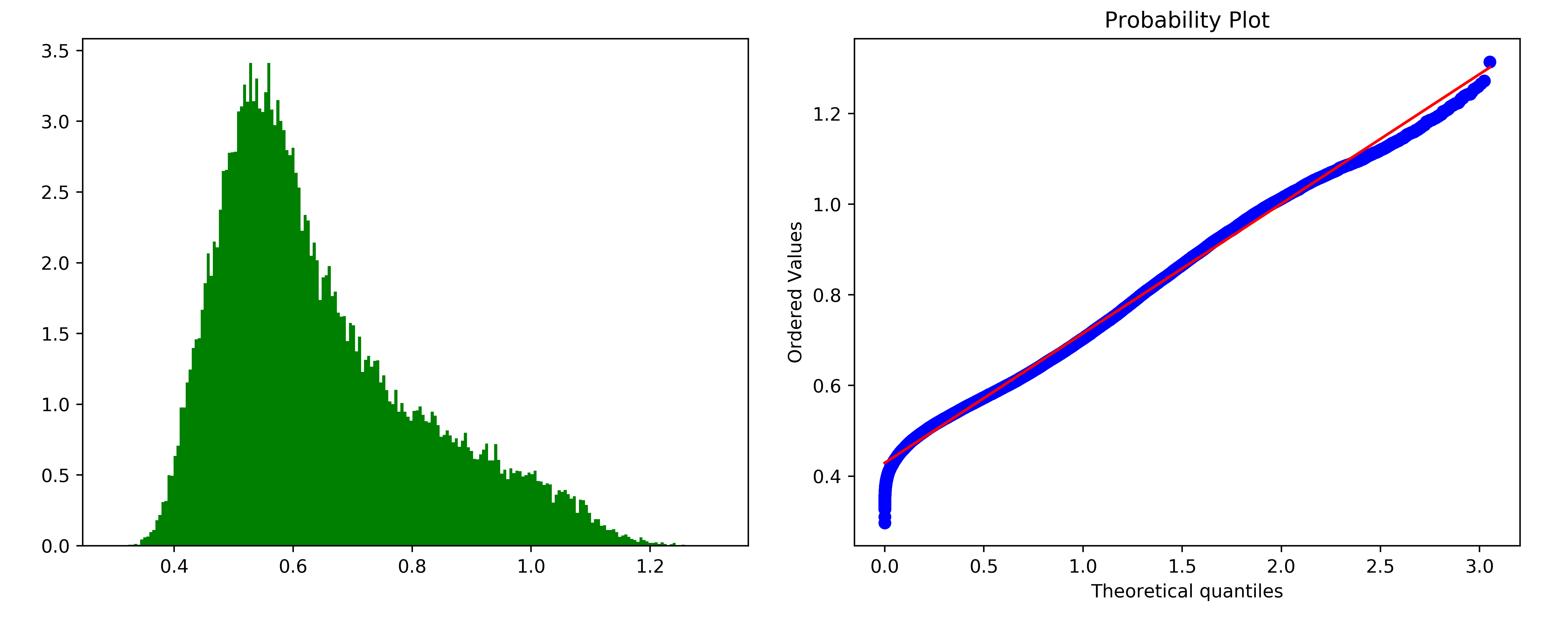
Figure 5: The histogram of the Euclidean distance from the projected semantic vector to the mean semantic vector for aeroplane class, and the Q-Q plot of the fitting GPD.

TABLE IX: Comparison with the method without projection distance loss on VOC 2007

Step	$\mathcal{L}_{pd}^{zsc}$					without $\mathcal{L}_{pd}^{zsc}$
	$\mathcal{G}_{1}$	$\mathcal{G}_{2}$	$\mathcal{G}_{3}$	$\mathcal{G}_{4}$	mAP	$\mathcal{G}_{1}$	$\mathcal{G}_{2}$	$\mathcal{G}_{3}$	$\mathcal{G}_{4}$	mAP
1	45.45	1.65	5.47	2.10	13.67	36.06	1.8	2.54	1.62	10.5
2	42.96	53.42	6.49	5.22	27.02	29.99	50.59	6.81	5.08	23.12
3	42.82	48.78	67.38	5.59	41.14	25.16	44.89	58.6	2.85	32.88
4	52.79	50.73	63.05	57.86	56.11	42.86	48.43	56.21	50.05	49.39

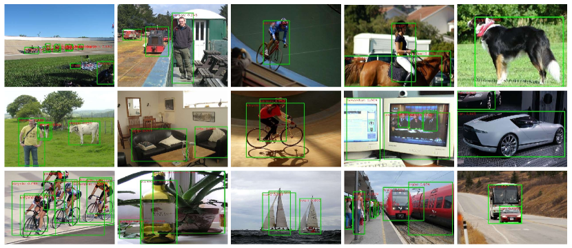
Figure 6: Qualitative Results of our IZSD-EVer on VOC 2007

V-F The effect of PD loss

To demonstrate the effect of PD loss, we compare the results of the model without PD loss. As shown in the Tab. IX, the performance of our model on all classes is better than the model without PD loss. This shows that using our proposed PD loss can maintain the ability to align the visual space and semantic spaces of old seen classes.

V-G The effect of $\alpha$ in $\mathcal{L}_{mse}$

The hyperparameter $\alpha$ in $\mathcal{L}_{mse}$ is used to alleviate extreme imbalance between background and foreground in region proposals generated by RPN. To demonstrate the impact of $\alpha$, we fixed other hyperparameters to evaluate the performance of our IZSD-EVer with different $\alpha=\{1,3,5,7\}$. As shown in Fig. 7(a), our IZSD-EVer with $\alpha=5$ performs the best for seen and unseen classes. Therefore, we set $\alpha=5$ in the main paper.

V-H The effect of $\beta$ in $\mathcal{L}_{zsc}$

$\beta$ is a hyperparameter to control the importance of $\mathcal{L}_{rec}$ loss. We also do comparative experiments to evaluate the effect of $\beta$ in $\mathcal{L}_{zsc}$. We fixed other hyperparameters and only changed the $\beta$ to $\{0.1,0.01,0.001,0.0001\}$. As shown in Fig. 7(b), our IZSD-EVer performs the best for seen and unseen classes where $\beta=0.001$. Therefore, we set $\beta=0.001$ in the main paper.

V-I The effect of $\gamma$ in $\mathcal{L}_{IL}$

The hyperparameter $\gamma$ controls the importance of $\mathcal{L}_{fd}^{rpn}$ in $\mathcal{L}_{IL}$. We do comparative experiments to evaluate the effect of $\gamma$. We fixed other hyperparameters and only changed the $\gamma$ to $\{1,2,5,10\}$. As shown in Fig. 7(c), our IZSD-EVer performs the best for seen and unseen classes where $\gamma=2$, which is consistent with the recommendation of Hao et al.. Therefore, we set $\gamma=2$ in the main paper.

V-J The effect of margin $m$ in $\mathcal{L}_{tri}$

The hyperparameter $m$ is the margin in the $\mathcal{L}_{tri}$. To demonstrate the impact of margin $m$, we fixed other hyperparameters and only changed the margin $m$ to $\{1,2,5,10\}$. As shown in the Fig. 7(d), as $m$ increases, the mAP of IZSD-EVer shows a slow downward trend. Our IZSD-EVer performs the best where $m=1$. Thus, we set $m=1$ in the main paper.

V-K The effect of $\delta$ in EVer

$\delta$ is the threshold used in EVer to distinguish whether the projected semantic vector comes from the seen classes or the unseen classes. To demonstrate the impact of $\delta$, we fixed other hyperparameters and only changed the $\delta$ to $\{0.01,0.02,0.05,0.1,0.2\}$. As shown in the Fig. 7(e), our IZSD-EVer performs the best where $\delta=0.02$, so we set $\delta=0.02$ in the main paper.

V-L The effect of memory size $K$

The bounded memory component $\mathcal{M}$ is introduced to alleviate the imbalance between old seen and new seen classes. To demonstrate the impact of memory size $K$, we fixed other hyperparameters to evaluate the performance of our IZSD-EVer with different $K=\{150,300,450,600\}$. As shown in the Fig. 7(f), as $K$ increases, the mAP of IZSD-EVer gradually increases. However, the memory size cannot be too large, especially for devices with limited storage capacity, so we set $K=150$ in the main paper.

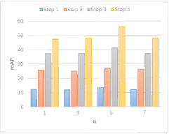
(a) The effect of $\alpha$

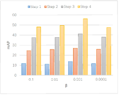
(b) The effect of $\beta$

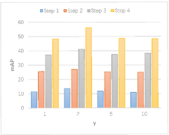
(c) The effect of $\gamma$

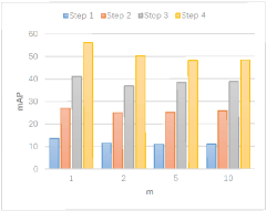
(d) The effect of margin $m$

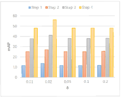
(e) The effect of $\delta$

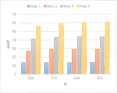
(f) The effect of memory size $K$

Figure 7: The effect of different hyperparameters on the performance of IZSD-EVer.The horizontal axis of each subgraph is the different value of the hyperparameter, and the vertical axis is the mAP of each step.

TABLE X: Classes splits for different datasets in different experiments

Dataset	Classes Split for Incremental Learning
	$\mathcal{G}_{1}$	$\mathcal{G}_{2}$	$\mathcal{G}_{3}$	$\mathcal{G}_{4}$
VOC 2007	aeroplane, bicycle, bird, boat, bottle	bus, car, cat, chair, cow	diningtable, dog, horse, motorbike, person	pottedplant, sheep, sofa, train, tvmonitor
COCO 2017	person, bicycle, car, motorcycle, airplane, bus, train, truck, boat, traffic light, fire hydrant, stop sign, parking meter, bench, bird, cat, dog, horse, sheep, cow	elephant, bear, zebra, giraffe, backpack, umbrella, handbag, tie, suitcase, frisbee, skis, snowboard, sports ball, kite, baseball bat, baseball glove, skateboard, surfboard, tennis racket, bottle	wine glass, cup, fork, knife, spoon, bowl, banana, apple, sandwich, orange, broccoli, carrot, hot dog, pizza, donut, cake, chair, couch, potted plant, bed	dining table, toilet, tv, laptop, mouse, remote, keyboard, cell phone, microwave, oven, toaster, sink, refrigerator, book, clock, vase, scissors, teddy bear, hair drier, toothbrush
	Classes Split for Zero-Shot Detection
	Seen Classes		Unseen Classes
VOC 2007 + VOC 2012	bus, sheep, chair, person, boat, cat, motorbike, bottle, bird, aeroplane, diningtable, cow, bicycle, pottedplant, tvmonitor, horse		car, dog, sofa, train
COCO 2014 48/17	toilet, bicycle, apple, train, laptop, carrot, motorcycle, oven, chair, mouse, boat, kite, sheep, horse, sandwich, clock, tv, backpack, toaster, bowl, microwave, bench, book, orange, bird, pizza, fork, frisbee, bear, vase, toothbrush, spoon, giraffe, handbag, broccoli, refrigerator, remote, surfboard, car, bed, banana, donut, skis, person, truck, bottle, suitcase, zebra		umbrella, cow, cup, bus, keyboard, skateboard, dog, couch, tie, snowboard, sink, elephant, cake, scissors, airplane, cat, knife
COCO 2014 65/15	person, bicycle, car, motorcycle, bus, truck, boat, traffic light, fire hydrant, stop sign, bench, bird, dog, horse, sheep, cow, elephant, zebra, giraffe, backpack, umbrella, handbag, tie, skis, sports ball, kite, baseball bat, baseball glove, skateboard, surfboard, tennis racket, bottle, wine glass, cup, knife, spoon, bowl, banana, apple, orange, broccoli, carrot, pizza, donut, cake, chair, couch, potted plant, bed, dining table, tv, laptop, remote, keyboard, cell phone, microwave, oven, sink, refrigerator, book, clock, vase, scissors, teddy bear, toothbrush		airplane, train, parking meter, cat, bear, suitcase, frisbee, snowboard, fork, sandwich, hot dog, toilet, mouse, toaster, hair drier

References

- [1] S. Rahman, S. Khan, and F. Porikli, “Zero-shot object detection: Learning to simultaneously recognize and localize novel concepts,” in Asian Conference on Computer Vision. Springer, 2018, pp. 547–563.
- [2] K. Shmelkov, C. Schmid, and K. Alahari, “Incremental learning of object detectors without catastrophic forgetting,” in Proceedings of the IEEE International Conference on Computer Vision, 2017, pp. 3400–3409.
- [3] H. Yu, F. Yanwei, J. Yu-Gang, and T. Qi, “An end-to-end architecture for class-incremental object detection with knowledge distillation,” in ICME, 2019.
- [4] P. Zhu, H. Wang, and V. Saligrama, “Zero shot detection,” TCSVT, 2019.
- [5] A. Bansal, K. Sikka, G. Sharma, R. Chellappa, and A. Divakaran, “Zero-shot object detection,” in ECCV, 2018.
- [6] S. Rahman, S. Khan, and N. Barnes, “Polarity loss for zero-shot object detection,” arXiv preprint arXiv:1811.08982, 2018.
- [7] ——, “Transductive learning for zero-shot object detection,” in Proceedings of the IEEE International Conference on Computer Vision, 2019, pp. 6082–6091.
- [8] Z. Li and D. Hoiem, “Learning without forgetting,” IEEE transactions on pattern analysis and machine intelligence, vol. 40, no. 12, pp. 2935–2947, 2017.
- [9] S.-A. Rebuffi, A. Kolesnikov, G. Sperl, and C. H. Lampert, “iCaRL: Incremental Classifier and Representation Learning,” in CVPR, 2017.
- [10] J. Kirkpatrick, R. Pascanu, N. Rabinowitz, J. Veness, G. Desjardins, A. A. Rusu, K. Milan, J. Quan, T. Ramalho, A. Grabska-Barwinska et al., “Overcoming catastrophic forgetting in neural networks,” Proceedings of the national academy of sciences, vol. 114, no. 13, pp. 3521–3526, 2017.
- [11] I. J. Goodfellow, M. Mirza, A. C. Da Xiao, and Y. Bengio, “An empirical investigation of catastrophic forgeting in gradientbased neural networks,” in In Proceedings of International Conference on Learning Representations (ICLR). Citeseer, 2014.
- [12] S. Liu, M. Long, J. Wang, and M. I. Jordan, “Generalized zero-shot learning with deep calibration network,” in NeurPIS, 2018.
- [13] S. Coles, J. Bawa, L. Trenner, and P. Dorazio, An introduction to statistical modeling of extreme values. Springer, 2001, vol. 208.
- [14] S. Ren, K. He, R. Girshick, and J. Sun, “Faster r-cnn: Towards real-time object detection with region proposal networks,” IEEE Transactions on Pattern Analysis and Machine Intelligence, vol. 39, no. 6, pp. 1137–1149, 2016.
- [15] G. Hinton, O. Vinyals, and J. Dean, “Distilling the knowledge in a neural network,” arXiv preprint arXiv:1503.02531, 2015.
- [16] J. Pickands III et al., “Statistical inference using extreme order statistics,” the Annals of Statistics, vol. 3, no. 1, pp. 119–131, 1975.
- [17] C. H. Lampert, H. Nickisch, and S. Harmeling, “Attribute-based classification for zero-shot visual object categorization,” PAMI, vol. 36, no. 3, pp. 453–465, 2014.
- [18] Y. Xian, Z. Akata, G. Sharma, Q. Nguyen, M. Hein, and B. Schiele, “Latent embeddings for zero-shot classification,” in CVPR, 2016.
- [19] J. Lei Ba, K. Swersky, S. Fidler et al., “Predicting deep zero-shot convolutional neural networks using textual descriptions,” in Proceedings of the IEEE International Conference on Computer Vision, 2015, pp. 4247–4255.
- [20] Z. Zhang and V. Saligrama, “Zero-shot learning via joint latent similarity embedding,” in CVPR, June 2016.
- [21] W.-L. Chao, S. Changpinyo, B. Gong, and F. Sha, “An empirical study and analysis of generalized zero-shot learning for object recognition in the wild,” in European Conference on Computer Vision. Springer, 2016, pp. 52–68.
- [22] Y. Xian, B. Schiele, and Z. Akata, “Zero-shot learning-the good, the bad and the ugly,” in ICCV, 2017.
- [23] B. Demirel, R. G. Cinbis, and N. Ikizler-Cinbis, “Zero-shot object detection by hybrid region embedding,” in BMVC, 2018.
- [24] F. M. Castro, M. J. Marín-Jiménez, N. Guil, C. Schmid, and K. Alahari, “End-to-end incremental learning,” in Proceedings of the European Conference on Computer Vision (ECCV), 2018, pp. 233–248.
- [25] E. Belouadah and A. Popescu, “Il2m: Class incremental learning with dual memory,” in The IEEE International Conference on Computer Vision (ICCV), October 2019.
- [26] Y. Wu, Y. Chen, L. Wang, Y. Ye, Z. Liu, Y. Guo, and Y. Fu, “Large scale incremental learning,” in The IEEE Conference on Computer Vision and Pattern Recognition (CVPR), June 2019.
- [27] R. Girshick, “Fast r-cnn,” in Proceedings of the IEEE international conference on computer vision, 2015, pp. 1440–1448.
- [28] C. L. Zitnick and P. Dollár, “Edge boxes: Locating object proposals from edges,” in European conference on computer vision. Springer, 2014, pp. 391–405.
- [29] W. J. Scheirer, A. Rocha, R. Michaels, and T. E. Boult, “Meta-recognition: The theory and practice of recognition score analysis,” IEEE Transactions on Pattern Analysis and Machine Intelligence (PAMI), vol. 33, pp. 1689–1695, 2011.
- [30] W. J. Scheirer, L. P. Jain, and T. E. Boult, “Probability models for open set recognition,” TPAMI, 2014.
- [31] W. J. Scheirer, Extreme Value Theory-Based Methods for Visual Recognition. Morgan & Claypool Publishers, February 2017.
- [32] E. Rudd, L. P. Jain, W. J. Scheirer, and T. Boult, “The extreme value machine,” IEEE Transactions on Pattern Analysis and Machine Intelligence (T-PAMI), vol. 40, no. 3, March 2018.
- [33] E. Vignotto and S. Engelke, “Extreme value theory for open set classification–gpd and gev classifiers,” arXiv preprint arXiv:1808.09902, 2018.
- [34] T. Mikolov, I. Sutskever, K. Chen, G. S. Corrado, and J. Dean, “Distributed representations of words and phrases and their compositionality,” in NIPS, 2013.
- [35] J. Pennington, R. Socher, and C. D. Manning, “Glove: Global vectors for word representation,” in Proceedings of the 2014 conference on empirical methods in natural language processing (EMNLP), 2014, pp. 1532–1543.
- [36] E. Kodirov, T. Xiang, and S. Gong, “Semantic autoencoder for zero-shot learning,” in Proceedings of the IEEE Conference on Computer Vision and Pattern Recognition, 2017, pp. 3174–3183.
- [37] A. A. Balkema and L. De Haan, “Residual life time at great age,” The Annals of probability, pp. 792–804, 1974.
- [38] M. Everingham, L. Van Gool, C. K. I. Williams, J. Winn, and A. Zisserman, “The Pascal Visual Object Classes (VOC) Challenge,” IJCV, 2010.
- [39] T.-Y. Lin, M. Maire, S. Belongie, L. Bourdev, R. Girshick, J. Hays, P. Perona, D. Ramanan, C. L. Zitnick, and P. Dollár, “Microsoft COCO: Common Objects in Context,” ArXiv, 2014.
- [40] Y. Fu, T. Xiang, Y.-G. Jiang, X. Xue, L. Sigal, and S. Gong, “Recent advances in zero-shot recognition: Toward data-efficient understanding of visual content,” IEEE Signal Processing Magazine, vol. 35, no. 1, pp. 112–125, 2018.
- [41] A. Farhadi, I. Endres, D. Hoiem, and D. Forsyth, “Describing objects by their attributes,” in CVPR, 2009.
- [42] K. He, X. Zhang, S. Ren, and J. Sun, “Deep residual learning for image recognition,” in Proceedings of the IEEE conference on computer vision and pattern recognition, 2016, pp. 770–778.