-statistics on bipartite exchangeable networks
Abstract
Bipartite networks with exchangeable nodes can be represented by row-column exchangeable matrices. A quadruplet is a submatrix of size . A quadruplet -statistic is the average of a function on a quadruplet over all the quadruplets of a matrix. We prove several asymptotic results for quadruplet -statistics on row-column exchangeable matrices, including a weak convergence result in the general case and a central limit theorem when the matrix is also dissociated. These results are applied to statistical inference in network analysis. We suggest a method to perform parameter estimation, network comparison and motifs count for a particular family of row-column exchangeable network models: the bipartite expected degree distribution (BEDD) models. These applications are illustrated by simulations.
keywords:
[class=MSC2020]keywords:
1 Introduction
RCE matrices
Networks arise naturally when considering interaction data. The nodes of a network represent the entities of a system and an edge between two nodes represents the interaction between the associated entities. The network is bipartite when there are two different sets of nodes, and edges only link nodes of different types. A natural representation for a bipartite network is its rectangular adjacency matrix. The rows and columns of an adjacency matrix represent the two different types of nodes and each entry encodes the interaction between the nodes associated to row and column , e.g. for binary networks, if and interact and else, or for weighted networks, is the weight of the edge linking and .
Many probabilistic network models assume that the network units, either edges or nodes, are exchangeable, i.e. are invariant by permutation. In the adjacency matrix of a bipartite network, the edge-exchangeability corresponds to the exchangeability of all its entries (full exchangeability), such as in Adamczak, Chafaï and Wolff (2016), while the node-exchangeability refers to the exchangeability of its rows and columns, such as in Aldous (1981).
Recent developments have been made for edge-exchangeable models (Cai, Campbell and Broderick, 2016; Williamson, 2016), but node-exchangeable models have a longer history for both unipartite and bipartite networks and encompasses families of models such as the stochastic block model (Holland, Laskey and Leinhardt, 1983; Snijders and Nowicki, 1997), the latent block model (Govaert and Nadif, 2003), the latent position model (Hoff, Raftery and Handcock, 2002) or the random dot product graph model (Young and Scheinerman, 2007). Implicitly, the exchangeability of the network units is associated with a sampling assumption. The choice of whether considering the exchangeability for edges or nodes depends on what is assumed to be sampled to observe the networks, whether it be edges or nodes (Crane and Dempsey, 2018).
Let us observe a bipartite network represented by a finite submatrix of size . We assume that the nodes of the same type are infinitely exchangeable, which means that the row elements and the column elements of the adjacency matrix are separately invariant under infinite permutation. The infinite exchangeability assumption is equivalent to considering that this observed network is made of the first rows and columns of an infinite adjacency matrix, whose rows and columns are exchangeable. This assumption is similar to Orbanz and Roy (2014) for unipartite networks and provides a consistent framework to analyze networks of different sizes. It can be used with many random network models, including the ones listed above (stochastic block model, latent block model, latent position model and random dot product graph model).
However, it has to be distinguished from the finitely exchangeable case. Finite exchangeability does not imply infinite exchangeability, for example, if the observed network consists of the first rows and columns of a larger adjacency matrix but of finite size. In that case, we say that the (finitely) exchangeable sequences of nodes are not infinitely extendible (Konstantopoulos and Yuan, 2019; Mai, 2020). The finitely exchangeable case for networks has been notably studied by Lauritzen, Rinaldo and Sadeghi (2018), but is out of scope of our paper. From here, the concept of exchangeability will always refer to infinite exchangeability, unless explicitely specified.
Thus, the exchangeability property of our infinite adjacency matrices is called row-column exchangeability. Let be the group of finite permutations over . An infinite matrix is said to be row-column exchangeable (RCE) if for any couple ,
where .
U-statistics
-statistics form a large class of statistics with interesting properties for many purposes such as estimation and hypothesis testing. We are interested in using them to analyze RCE networks.
Given a sequence of random variables numbered with a unique index, a -statistic is defined as the following average
| (1) |
where is a symmetric function of size referred to as the kernel.
The case where the are i.i.d. is well-studied. Halmos (1946) established the optimality of -statistics as unbiased estimators and Hoeffding (1948) derived a central limit theorem (CLT), which ensures their asymptotic normality provided . For dependent cases, results exist for several dependency strucures, for example Nandi and Sen (1963); Zhao and Chen (1990) for finitely exchangeable variables, Reitzner and Schulte (2013) for Poisson point processes or Duchemin, De Castro and Lacour (2020, 2022) for Markov chains.
In the infinitely exchangeable case, it is particularly convenient to view as an array of random variables indexed by -tuples where . With this notation, it becomes clear that the -statistic defined by (1) is the sum of the corresponding entries of the -dimensional array . But being exchangeable implies that the array is jointly exchangeable, i.e. it is invariant by the action of joint permutations on each of its indices, for any sequence of -tuples and for any finite permutation ,
| (2) |
Eagleson and Weber (1978) proved a CLT for sums jointly exchangeable arrays, which applies to -statistics of exchangeable sequences. Many other asymptotic results for -statistics of exchangeable sequences were derived afterwards, such as a Berry-Esseen bound (van Zwet, 1984) and a law of iterated logarithm (Scott and Huggins, 1985).
In relation with the existing literature, we add here the definition of separate exchangeability. is said to be separately exchangeable if for any sequence of -tuples and for any permutations of ,
| (3) |
-statistics for RCE matrices
Our contribution applies to -statistics based on submatrices of size , that we call quadruplets, of an (infinite) RCE matrix
Their kernels are real functions over quadruplets. To mimic the kernel symmetry in the unidimensional case, we assume that they present the following symmetry property: for any matrix ,
| (4) |
This assumption can be made without loss of generality for -statistics, since any quadruplet function can be made symmetric considering
and .
Applied to an observed network represented by the first rows and columns of , a quadruplet -statistic is then defined by
| (5) |
where is the number of -combinations from elements. For clarity, we define the -dimensional array using the following notation
which means that a -statistic is the mean of the first entries of . However, -statistics of jointly exchangeable arrays deal with the mean of the first entries of the array . Therefore, Theorem 4 of Eagleson and Weber (1978) applies to -statistics of square matrices, but not generally to the case of bipartite networks, where row and column nodes are distinct by nature. In particular, -statistics for RCE matrices allow row and column indices to overlap and most importantly, to be different from . Instead, the invariance structure of is a special case of -exchangeability (Kallenberg, 1999), where for any two permutations and of , we have
| (6) |
Therefore, is not separately exchangeable because, compared to (3), the same permutation has to be applied on both row indices and and the same permutation on both column indices and .
Lemma 12 of Kallenberg (1999) establishes a strong law of large numbers for -exchangeable variables, which applies to our -statistics. Our aim is to establish a weak convergence theorem similar to Theorem 4 of Eagleson and Weber (1978). In the recent literature, two related results were obtained by Austern and Orbanz (2022) and Davezies, D’Haultfœuille and Guyonvarch (2021). Austern and Orbanz (2022) explains how a result from Lindenstrauss (1999) can be translated to a strong law of large numbers for sums of exchangeable arrays and their Theorem 17 is analogous to Theorem 4 of Eagleson and Weber (1978) but it is obtained using Stein’s method. Davezies, D’Haultfœuille and Guyonvarch (2021) adopted a functional point of view. Their Theorem 2.1 is a Donsker-type version of the same result on jointly exchangeable arrays and Theorem 3.4 is an extension to separately exchangeable arrays. Because -statistics of jointly exchangeable arrays are not suited to bipartite networks and because our arrays are not separately exchangeable, these results do not apply to our -statistics of RCE matrices, as defined in (5) where (6) is satisfied.
To generalize these results to our case, our proof relies on the convergence of sums of backward martingales (Theorem 1 of Eagleson and Weber, 1978). We derive a CLT result in the case where the RCE matrix is dissociated, i.e. any of its submatrices with disjoint indexing sets are independent. This CLT excludes the degenerate case (i.e. when the convergence rate to the limiting distribution is greater than , see Section 4) through a clear assumption on the asymptotic variance. In the degenerate case, the convergence result of Austern and Orbanz (2022) does not lead to a CLT neither, and Davezies, D’Haultfœuille and Guyonvarch (2021) proved a different convergence theorem. We offer a discussion on the degenerate case and its implications in Section 4. Finally, we recall that the backward martingale approach also yields Kallenberg’s strong law of large numbers (Kallenberg, 1999).
In the last part of this work, we will put a special emphasis on the statistical analysis of bipartite networks. We introduce two versions of a RCE matrix model, the Bipartite Expected Degree Distribution (BEDD) model and we explain how our theorems apply to both of them. We suggest a method to perform statistical inference on these models using quadruplet -statistics through several examples and we discuss how one can extend it.
Outline
The weak convergence theorem in the general case and the CLT in the dissociated case are presented and proven in Section 2. We shed further light on the difference between the dissociated and the non-dissociated cases using the Aldous-Hoover representation theorem. Section 3 illustrates our results with applications to statistical network analysis using a RCE model and several examples of inference tasks.
2 Main result
2.1 Asymptotic framework
Our results apply in an asymptotic framework where the numbers of rows and columns of the submatrix used in the calculation of the -statistic grow at the same rate, i.e. . To simplify the proofs, we allow only one row or one column to be added to the submatrix. Now, we build a sequence of dimensions for the submatrix satisfying these conditions.
Definition 2.1 (Sequence of dimensions).
Let be an irrational number such that . For all , we define and , where is the floor function.
Proposition 2.2.
and satisfy:
-
1.
,
-
2.
, for all .
Corollary 2.3.
At each iteration , one and only one of these two propositions is true:
-
1.
and ,
-
2.
and .
2.2 Theorems
We establish the following results on the asymptotic behaviour of -statistics over RCE matrices.
Theorem 2.5 (Main theorem).
Let be a RCE matrix. Let be a quadruplet kernel such that . Let be the sequence of -statistics associated with defined in Definition 2.4. Let and . Set and
If , then
where is a random variable with characteristic function .
Theorem 2.5 states that the limiting distribution of is a mixture of Gaussians. consists of two terms corresponding to the covariance of the kernel taken on two quadruplets sharing one row or one column, conditional on . The condition is used to avoid the case almost surely, which is a degenerate case discussed in Section 4. Since is not constant in general, the limit distribution is an infinite mixture of Gaussians. This expression is analogous to in Theorem 4 of Eagleson and Weber (1978) for jointly exchangeable arrays and the covariance kernel in Theorems 2.1 and 3.4 of Davezies, D’Haultfœuille and Guyonvarch (2021) for jointly and separately exchangeable arrays. We see that if is constant, then the asymptotic distribution is a simple Gaussian. One may observe that and studied in Corollary 19 of Austern and Orbanz (2022) are related as when and . Still the convergence rates given in Theorem 2.5 and Corollary 19 of Austern and Orbanz (2022) (the proof of which is not given in the paper) are inconsistent. From what we understand, Corollary 19 actually corresponds to a degenerate case () in Theorem 2.5. Next we identify a class of models where the limiting distribution of is a simple Gaussian.
Definition 2.6.
is a dissociated matrix if and only if is independent of , for all and .
In other words, is dissociated if submatrices that are not sharing any row or column are independent. Now we claim the following extension to Theorem 2.5 for dissociated RCE matrices.
Theorem 2.7.
In addition to the hypotheses of Theorem 2.5, if is dissociated, then and are constant and
More precisely,
-
1.
,
-
2.
.
This result can be more directly exploited for statistical applications, as the limiting distribution is much more simple. Another important result is the joint asymptotic normality of -statistics, which holds as long as Theorem 2.7 applies to each kernel separately and they are linearly independent.
Theorem 2.8.
This theorem allows us to obtain the asymptotic normality of linear combinations of -statistics and more interestingly, the asymptotic normality of differentiable functions of -statistics (see Section 3.2).
Remark.
Lemma 12 of Kallenberg (1999) already provided a strong law of large numbers for -exchangeable arrays, of which quadruplet kernels are a subcase. The following theorem rephrases Kallenberg’s law of large numbers for quadruplet -statistics and gives an additional precision in the dissociated case for which we provide an alternative proof, as it is a natural consequence of our proof of Theorems 2.5 and 2.7.
Theorem 2.9.
Let be a RCE matrix. Let be a quadruplet kernel. Let the sequence of -statistics associated with defined in Definition 2.4. Let and . We have
Furthermore, if is dissociated, then .
2.3 The Aldous-Hoover theorem
We shall explain Theorems 2.5 and 2.7 in the light of the Aldous-Hoover representation theorem. Theorem 1.4 of Aldous (1981) states that for any RCE matrix , there exists a real function such that if we denote , for , where the , , and are i.i.d. random variables with uniform distribution over , then
| (7) |
It is possible to identify the role of each of the random variables involved in the representation theorem. We notice that each is determined by and . is entry-specific while is shared by all the entries involving the row and by the ones involving the column . Therefore, the and represent the contribution of each individual of type 1 and type 2 of the network, i.e. each row and column of the matrix. These contributions are i.i.d., which makes the network exchangeable. Finally, is global to the whole network and shared by all entries.
Proposition 3.3 of Aldous (1981) states that if is dissociated, then can be written without , i.e. it is of the form , for . In this case, because the , and are i.i.d., averaging with the -statistic over an increasing number of nodes nullifies the contribution of each individual interaction () and node ( and ). In the general case, i.e. when is not dissociated, then conditionally on , is dissociated. It is easy to see that the mixture of Gaussians from Theorem 2.5 results from this conditioning.
In practice, dissociated exchangeable random graph models are widely spread. Notably, a RCE model is dissociated if and only if it can be written as a -graph (or graphon), i.e. it is defined by a distribution depending on two parameters in such that for :
see Diaconis and Janson (2008) for binary bipartite graphs, Lovász and Szegedy (2010) for an extension to weighted graphs but in a unipartite setup. In this definition, it is easy to recognize the variables from the representation theorem of Aldous-Hoover. We simply identify the and , then it suffices to take the inverse distribution function of to see that defining the dissociated RCE matrix such that fulfills .
2.4 Proof of Theorem 2.5
To prove Theorem 2.5, we adapt the proof of Eagleson and Weber (1978) establishing the asymptotic normality of sums of backward martingale differences. The definition of a backward martingale is reminded in Appendix B.
Theorem 2.10 (Eagleson and Weber, 1978).
Let be a square-integrable reverse martingale, a -measurable, a.s. finite, positive random variable. Denote where . Set . If:
-
1.
(asymptotic variance),
-
2.
for all , (conditional Lindeberg condition),
then , where is a random variable with characteristic function .
Proof of Theorem 2.5.
The three steps to apply Theorem 2.10 to are to show that it is a backward martingale for a well chosen filtration and that it fulfills conditions and . The expression of is made explicit along the way. More precisely,
-
1.
first, defining , Proposition C.1 states that is indeed a square-integrable reverse martingale ;
-
2.
then, Proposition D.1 implies that , where , does converge to a random variable with the desired expression ;
-
3.
finally, the conditional Lindeberg condition is ensured by Proposition E.1, since from it, we deduce that for all , .
Hence, if is positive, Theorem 2.10 can be applied to and we obtain that , where is a random variable with characteristic function . The proofs of Propositions C.1, D.1 and E.1 are provided in Appendices C, D and E respectively. ∎
2.5 Proof of Theorem 2.7
The proof of Theorem 2.7 relies on a Hewitt-Savage type zero-one law for events that are permutable in our row-column setup. Therefore, it is useful to define first what a row-column permutable event is. We remind the Aldous-Hoover representation theorem for dissociated RCE matrices as stated earlier: if is a dissociated RCE matrix, then its distribution can be written with , and arrays of i.i.d. random variables.
Then let us consider such arrays of i.i.d. random variables , and . If we were to consider events depending only on them, there is no loss of generality in using the product probability space , where
We then define the action of a row-column permutation on an element of .
Definition 2.11.
Let . The action of on is defined by
where , and
Definition 2.12.
Let . is invariant by the action of if and only if for all , , i.e.
Notation.
In this section, we denote by the collection of events of that are invariant by row-column permutations of size , i.e. . We denote , which is the collection of events that are invariant by permutations of size , for all .
The following theorem is an extension of the Hewitt-Savage zero-one law to the row-column setup.
Theorem 2.13.
For all , or .
The proof of Theorem 2.13 is given in Appendix F. Now we use this result to derive Theorem 2.7 from Theorem 2.5.
Proof of Theorem 2.7.
In this proof, we specify the matrices over which the -statistics are taken, i.e. for a RCE matrix , we denote instead of the -statistic of size with kernel taken on , given by formula (5), and analogously and . We denote also which are sets of events depending on , and .
Since is RCE and dissociated, Proposition 3.3 of Aldous (1981) states the existence of a real function such that for , and , where , and , for are i.i.d. random variables with uniform distribution on . Therefore we can consider such function and these random variables, the product spaces and the sets of invariant events defined earlier.
But , so for all , . It follows that , so is -measurable. Theorem 2.13 states that all the events in happen with probability 0 or 1, so it ensures that is constant. Moreover, since the distribution of is the same as this of , we can conclude that .
Likewise, we deduce that and which gives the desired result for . Thus we conclude that of Theorem 2.5 follows a Gaussian distribution of variance .
∎
2.6 Proof of Theorem 2.8
The proof of Theorem 2.8 relies on the Cramér-Wold theorem (see Theorem 29.4 of Billingsley, 1995). If is enough to show that any linear combination of -statistics converges to the corresponding linear combination of their limits.
Proof of Theorem 2.8.
Let be a vector of random variables following a centered multivariate Gaussian distribution with covariance matrix defined in the theorem. Then for all and for all and .
For some , we set . First, assume that . Then by hypothesis, , therefore is a -statistic with quadruplet kernel . Using Cauchy-Schwarz inequality and the fact that for all , we have furthermore
Therefore, Theorem 2.7 also applies for and , where and with since Theorem 2.7 applies. This means that .
Now assume that . Then so . Therefore, is still true.
We have proven that for all , so we can finally apply the Cramér-Wold theorem (Theorem 29.4 of Billingsley, 1995) which states that converges jointy in distribution to , which is a centered multivariate Gaussian with covariance matrix , so this concludes the proof. ∎
2.7 Proof of Theorem 2.9
The proof for the first part of the theorem can be derived from the proof of Proposition C.1, without needing the hypothesis . Indeed, it is enough to show that is a (not necessarily square-integrable) backward martingale and to apply Theorem B.3.
As for the dissociated case, is ensured by the proof of Theorem 2.7.
3 Applications
In this section, we illustrate how the results from the previous section can be used for statistical inference for network data through different examples. First, we introduce the Bipartite Expected Degree Distribution (BEDD) models, a family of RCE models and we show how Theorems 2.5 and 2.7 apply. Then, we detail three examples to show how one might exploit the -statistics properties to analyze networks. In the first example, we use different quadruplet kernels to estimate the row heterogeneity of a network, with the help of the delta-method. Next, we extend this example to build a statistical test to compare the row heterogeneity of two networks. In the last example, we use -statistics to estimate the frequency of network motifs.
3.1 The BEDD model
General model
As examples of models for RCE matrices, we consider the family of the BEDD models, which are weighted, bipartite and exchangeable extensions of the Expected Degree Sequence model (Chung and Lu, 2002; Ouadah, Latouche and Robin, 2022). For binary graphs, the degree of a node is the number of edges that stem from it. For weighted graphs, the equivalent notion is the sum of the weights of these edges. It is sometimes called node strength (Barrat et al., 2004), but we will simply refer to it as node weight. A BEDD model draws the node weights from two distributions, characterised by càdlàg, non-decreasing and bounded real functions and of . The expected edge weights are then proportional to the expected weights of the involved nodes. A BEDD model can be written in a hierarchical form
| (8) |
where given any real number , we denote by a family of probability distributions with expectation and finite variance, is a positive real number and and are normalized by the condition . For a graph of size , conditionally to , and , the expected weight of the -th row is and the expected weight of the -th column is . Consequently, is the mean intensity of the network. One can define different BEDD models by specifying different families of distributions . For a family , we refer to the -BEDD model (e.g. Poisson-BEDD or Bernoulli-BEDD).
Furthermore, we define two versions of BEDD models:
- Version 1
-
is constant,
- Version 2
-
is a random variable.
By construction, the BEDD models are RCE, so Theorem 2.5 can be applied to matrices generated by these two versions of BEDD models. Theorem 2.7 only applies to Version 1, where the matrix is dissociated. Indeed, we see that in both models conditionally on , the expected mean of the interactions of any submatrix is . Therefore any 2 submatrices are independent if is constant. We could also have noticed that is determined by the from the representation theorem of Aldous-Hoover, see equation (7). As a remark, it is straightforward that unlike Version 2, Version 1 of BEDD models can be written as a -graph model as in Formula (2.3), setting .
Since Theorem 2.7 only applies to Version 1, we will be only considering this version in the rest of the article.
Definition 3.1.
Given a family of distributions a family of probability distributions with expectation and finite variance, a -BEDD model is a semi-parametric model described by the triplet where
-
1.
,
-
2.
and are real functions and of which are bounded, càdlàg, non-decreasing and normalized with .
We call the BEDD parameters and the matrix generated by a -BEDD model with these parameters is written and is described by (8), for all .
In this definition, the normalizing constraint on ensures that for all . The boundedness of and ensures that the variables and are bounded and their moments exist. In the binary case (Bernoulli-BEDD), it also puts a condition on . Since , the condition must hold. The non-decreasing and càdlàg conditions are similar to the condition of Bickel and Chen (2009) for their random graph model and ensures the identifiability of the model since otherwise, and could be replaced with any and , where and are measure-preserving transformations.
Identifiability by a quadruplet
In addition to being a dissociated RCE model, the BEDD models are particularly well adapted to use of quadruplet -statistics. In this paragraph, we show that for some choices of such as the Poisson distribution, the model can be recovered by a single quadruplet. We use the following two theorems of which proofs are given in Appendix G. The first theorem implies that the functions and of the BEDD models are characterised by their moments and .
Theorem 3.2.
Let be BEDD parameters and for some family of distributions . The distribution of is uniquely determined by , and , where and for all .
Now we specify an assumption on the family of distributions , under which a quadruplet identifies the parameters of a BEDD model.
Assumption 3.3.
For the family of distributions , there exists a sequence of functions such that if a random variable , then for every ,
This assumption holds for many usual distributions families such as the Poisson or the Binomial distributions. As an example, if follows a Poisson distribution, we have . This assumption does not hold for the Bernoulli distribution, as if , for any function , . This assumption is a sufficient condition to be able to recover the BEDD parameters from the joint distribution of a quadruplet.
Theorem 3.4.
If Assumption 3.3 holds for the family of distributions , then for all , and are uniquely determined by the joint distribution of a quadruplet.
This theorem suggests that all the BEDD information is contained in the distribution of a quadruplet, therefore it is possible to extract any information only with quadruplet kernels. Quadruplet -statistics are then especially of interest.
3.2 Heterogeneity in the row weights of a network
In this first example, we are interested in evaluating the heterogeneity of the row weights of a network. In the BEDD models, conditional to the latent variables following a uniform distribution on , the expected weights of the row nodes are given by the , as seen in Section 3.1. Therefore, the heterogeneity of the rows, i.e. the variance of the expected weight of a row node can be quantified by . In the example of an interaction network, if is constant, i.e. and , then the expected weight is constant for all rows and the row weight distribution is homogeneous, with all the row individuals having around the same number of interactions. Besides, the higher is, the more this distribution is unbalanced. In ecology, a large value of indicates a strong distinction between generalist (with high degree) and specialists (with low degree) species.
can be estimated using where and are the -statistics based on the quadruplet kernels and defined as
and
Proposition 3.5.
Let be defined as above. Then
| (9) |
where
| (10) |
and for all , and .
This result comes from the composition of the asymptotic normality of two -statistics. In the following, we show how to obtain equations (9) and (10). First, we see that and . So applying Theorem 2.7 successively to and gives the following results ( and are derived in Lemmas H.3 and H.4):
| (11) |
and
| (12) |
where
| (13) |
and
| (14) |
To combine the results (11) and (12), we apply Theorem 2.8 to . We find that
| (15) |
with
where . The derivation of is given by Lemma H.5. We suggest two methods to derive the weak convergence result for .
First method: the delta-method
The first-order Taylor expansion of at the point is
where is the gradient of and .
Second method
The delta-method is a generic method that applies to all differentiable functions . However, for our particular case, there is another way to find the same confidence intervals without using the delta-method. Let . One could have noticed that (15) also implies
where . This can be rewritten
| (16) |
Since , then Slutsky’s theorem yields equations (9) and (10).
Confidence intervals
In order to exploit equations (9) and (10), we have to estimate the remaining unknown quantities , , and . We use the kernels , , and listed in Table 1. Using equation (10) and two additional -statistics and based on the kernels and defined in Table 1, we build a consistent estimator for , defined as
| (17) |
Finally, it follows from Slutsky’s theorem that
| (18) |
From this result, one can derive the following asymptotic confidence interval at level for using the -th percentile of the standard normal distribution: for ,
| (19) |
Simulations
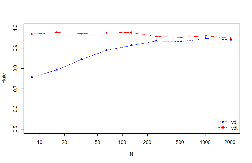
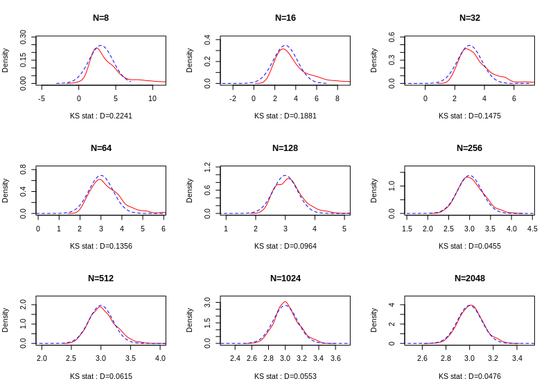
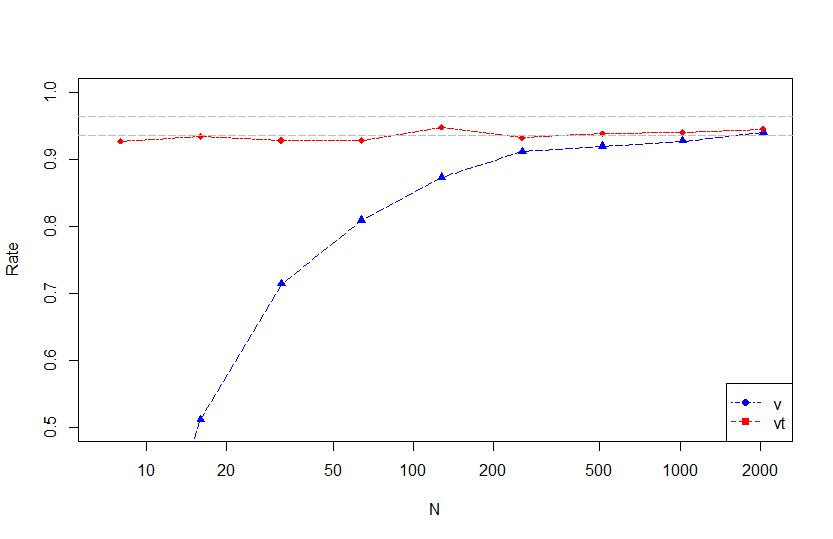
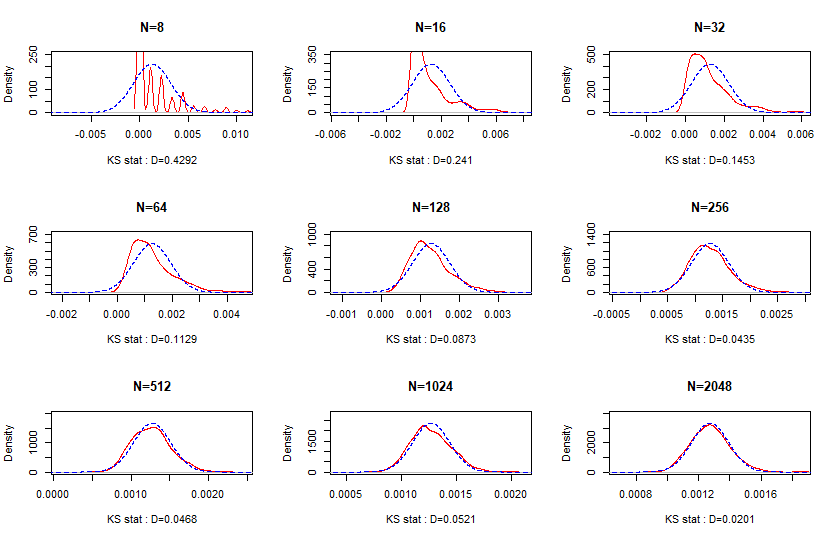
To illustrate this example, we have simulated networks with the Poisson-BEDD model. We have chosen power functions for and , i.e. we have set and in and and . Therefore, the values of and can be set by and . The constant is set at , so we have considered square matrices (). Figure 1 represents the frequency with which 2 confidence intervals, built with respectively equations (9) and (18) for , contain the true value of . The curve associated with suggests that becomes close to its limiting distribution for . For smaller values of , the frequencies are significantly higher than , so the confidence intervals are slightly larger than they should. The curve associated with suggests that underestimates , but using Slutsky to plug in for in (18) still leads to acceptable frequencies that converge when grows, especially for . Figure 2 represents the empirical distribution of for different sizes . It confirms that converges quickly to a normal distribution with variance .
3.3 Network comparison
Some methods have been developed to compare networks. Network statistics, graph spectra, network motifs or graph alignment methods can be used to build a distance (or similarity scores) between two networks (Emmert-Streib, Dehmer and Shi, 2016; Tantardini et al., 2019). In the context of random networks, fewer comparison methods rely on generative random graph models and they are relatively recent (Asta and Shalizi, 2015; Maugis et al., 2020). A model-based approach offers two advantages. First, by suggesting a distribution on the networks, one might be able to design a distance with known distribution and therefore use statistical tests to compare networks. Second, the use of a generative model makes it considerably easier to interpret, one can use to the model parameters to design a suitable distance to compare the networks, giving insights into the underlying process generating them. Such ability to interpret is particularly interesting in applications such as ecology, where it is crucial to understand how and why the networks differ (Pellissier et al., 2018). In this section, we show how one can extend the usage of -statistics to network comparison, providing a framework for model-based network comparison.
In the previous example, our analysis has been carried out on a single network. Now, consider two independent networks and and we wish to compare their row heterogeneity. Assume that they are respectively generated by the BEDD parameters and . Then, each network is associated with their respective values and . The data consists in two observed networks and , which are assumed to be extracted from the first (respectively ) rows and (respectively ) columns of the infinite matrices and . We would like to perform the following test: vs. using the two observed networks.
General method
Let . Suppose that . Then one can simply notice that , where is the estimator of Proposition 3.5 taken on the matrix , is still asymptotically normal from equation (9)
with and for BEDD parameters , is given by (10).
Using the estimators stemming from the delta-method (17), we build a consistent estimator for
Hence, Slutsky’s theorem ensures that
In this example, we consider the statistical test vs. . So we use the test statistic
| (20) |
for which Slutsky’s theorem applies
Under , which allows us to build asymptotic acceptance intervals for this test at level with the percentile of the standard normal distribution:
Simulations
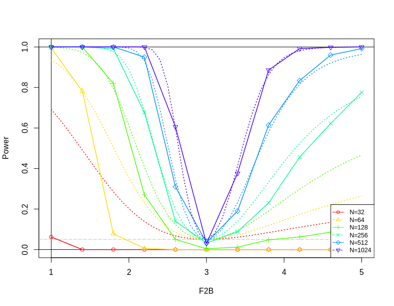
Figure 3 shows simulation results for this test. Once again, we consider networks generated by the Poisson-BEDD model with power law functions and . To perform the test, we generate couples of observed networks with fixed and identical and . is also fixed, but we let vary by setting the parameter of the power law, which is used to set . The empirical power for this test with varying is evaluated for several values of . It is compared with the asymptotic theoretical power for this test. Let . If a random variable is such that , then , so it can be computed with
| (21) |
where is the cumulative distribution function of a Gaussian variable with mean and variance . We notice that the empirical power becomes very close to the asymptotic theoretical power as grows, which suggests that this test works well for networks with .
3.4 Motif frequencies
A motif is a small-size subgraph. The frequencies of occurences of motifs (sometimes called network moments) are widely studied in network theory. Motifs frequencies have known asymptotic distribution under many generative models, so they can be used to analyze binary networks (Stark, 2001; Picard et al., 2008; Reinert and Röllin, 2010; Bickel, Chen and Levina, 2011; Bhattacharyya and Bickel, 2015; Levin and Levina, 2019; Maugis et al., 2020; Naulet et al., 2021; Ouadah, Latouche and Robin, 2022). Many probabilistic graph models also rely on motif frequencies, such as the Exponential Random Graph Model (Frank and Strauss, 1986) or the dk-random graphs (Orsini et al., 2015). For many real networks, one can interpret the frequencies of certain motifs, see examples for transcriptional networks (Shen-Orr et al., 2002), protein networks (Pržulj, Corneil and Jurisica, 2004), social networks (Bearman, Moody and Stovel, 2004), evolutionary trait networks (Przytycka, 2006), ecological food webs (Bascompte and Melián, 2005; Stouffer et al., 2007), ecological mutualistic networks (Baker et al., 2015; Simmons et al., 2019).
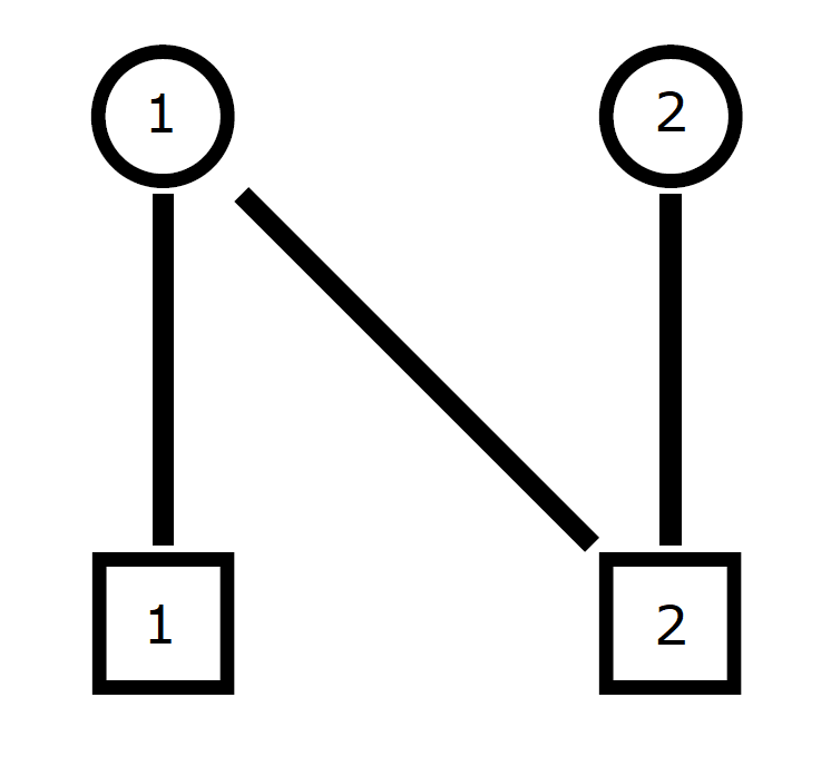
It naturally arises that frequencies of bipartite motifs of size can be expressed as quadruplet -statistics and can be integrated in our framework. If is a binary adjacency matrix, then one can count the motifs using a kernel and obtain statistical guarantees. For example, the motif represented in Figure 4 can be counted with the kernel
Theorem 2.7 shows that the associated -statistic converges to the theoretical frequency of this motif given the network model and it is asymptotically normal. Suppose , where are BEDD parameters, then
| (22) |
where following derivations given in Lemma H.6, and
The quantities , and appearing in the expression of the asymptotic variance can be consistently estimated using -statistics of larger subgraphs. For any , define the kernel of submatrices of size as follows:
Then the -statistic associated to is
Lemma H.7 states that and . Since is a RCE matrix, Kallenberg’s law of large number (Lemma 12 of Kallenberg, 1999) applies to these -statistics and and .
Using these consistent estimators for , and the and , we build an example of consistent estimator for
This expression may seem complex at first, however it is computationally simple as one only needs to compute for and for which can be easily done (see Appendix I).
From Slutsky’s theorem, it follows that
| (23) |
This result can be used to build asymptotic confidence intervals for the motif frequency , like in the previous examples of Sections 3.2 and 3.3.
Simulations
We simulate networks with the Bernoulli-BEDD model, with power law functions for and , similar to which of previous examples. For and in , and . and can be used to set and . and also determine the maximum value for , as we should have . The constant remains at .
Figure 5 represents the frequency with which the 2 confidence intervals built from equations (22) and (23) contain the true value of the target motif frequency . We see that as grows larger than , the frequency becomes very close to , although the variance is still underestimated until . In contrast to the example of Section 3.2, the frequencies for smaller than are very low ( and lower). This is an expected result as the estimator counts the motifs contained in the networks. The maximum number of motifs in the network is . For a fixed , can only take discrete values in . The support of is more and more restricted as becomes smaller, which makes the empirical distribution of more dissimilar from a Gaussian distribution.
This is also reflected in Figure 6 as the discrete support still appears very clearly in the yet smoothed distribution density of for and . Nevertheless, we see that the empirical distribution converges quickly to a Gaussian distribution, even faster than in the estimation example of Section 3.2, as the Kolmogorov-Smirnov statistics are smaller if is larger than .
4 Discussion
In this paper, we have proven a weak convergence result for quadruplet -statistics over RCE matrices, using a backward martingale approach. We use the Aldous-Hoover representation of RCE matrices and a Hewitt-Savage type argument to extend this result and obtain a CLT in the dissociated case. Using this CLT, we provide a general framework to perform statistical inference on bipartite exchangeable networks through several examples.
Indeed, -statistics can be used to build estimators. The advantage of taking quadruplets is to define functions over several interactions of the same row or column. This allows us to extract information on the row and column distribution. The CLT then guarantees an asymptotic normality result of the estimators, where the only unknown is their asymptotic variances, which have to be estimated then plugged in with Slutsky’s theorem.
Computational cost
One interesting feature of the kernels chosen in Section 3 is their computational simplicity. This simplicity comes naturally when considering quadruplet kernels consisting of small products. Indeed, if we denote , one can write and used in the estimation example (Sections 3.2 and 3.3) as
| (24) |
where is the trace operator. We see that and can be computed using only basic operations on matrices, which are optimized in most computing software. This can also be said for all the other -statistics used in this example, and by extension for the estimators and . Expressions for the remaining -statistics are given in Appendix I.
In the motif count example (Section 3.4), the -statistic can also be easily computed, despite the being kernels over submatrices larger than a quadruplet (at least one dimension greater than 2). The -statistics normally involve more complex summations but fortunately, we show in Appendix I that simpler expressions can be found for or .
Other models: graphons
We have seen that for a class of BEDD models (those falling under Assumption 3.3), the quadruplet -statistics are particularly interesting because a single quadruplet contains all the information of the model. The Bernoulli-BEDD used in Section 3.4 is an example of model where this assumption does not hold. Still, one can build estimators, apply Theorem 2.7 and perform statistical inference on this model, like in Section 3.4. In fact, the only conditions on the model are that it should be RCE and dissociated, i.e. it can be written as a bipartite W-graph model (see Section 2.3). For example, given the W-graph model with , one could have tested if it is of product form, i.e. if can be written as (as in the BEDD models). An appropriate kernel for this test would be
as with and and should be equal to 0 if the hypothesis is true.
Extension to larger subgraphs
It is legitimate to wonder if one can extend our framework to -statistics over submatrices of size different from , for example of size , i.e.
Such generalization opens up many possibilities by building new estimators.
First, as seen in Section 3.4, in the Bernoulli-BEDD model, the quantities and cannot be retrieved by a quadruplet for , but can be retrieved with subgraphs of size and with subgraphs of size . Second, our framework can also be used to count motifs of size larger that , since the maximum size of the motifs is determined by the size of the kernel. Finally, in the row heterogeneity example where we used formula (11) to derive an asymptotic confidence interval for , we notice that one could have estimated the term appearing in with a kernel over submatrices of size such as and .
Actually, our theorem can be extended to -statistics over larger subgraphs under similar conditions. All the steps of our proof can be adapted to -statistics of larger subgraphs. These -statistics are indeed backward martingales and the equivalent of Propositions D.1 and E.1 require more calculus. As a consequence, the asymptotic variance also has a different expression. On the one hand, such an extension would allow more flexibility in the choice of the kernel, hence the ability to build more complex estimators that are asymptotically normal. On the other hand, in practice, the computation of such -statistics may also be more complex and computationally demanding, whereas simple functions on quadruplets can easily be expressed with matrix operations.
Degeneracy
Degenerate cases are of interest because they are rather common. The degeneracy depends on the kernels and the distribution of . As an example, assume that one is interested to test vs. for a Poisson-BEDD model. Under , whereas under , . We plan to use the same estimator of than in Section 3.2. Equation (16) of the second method could be also obtained applying Theorem 2.7 to the kernel . From equation (10), we see that from that the asymptotic variance under , since . Thus, under , this is a degenerate case and Theorem 2.7 does not apply and the limiting distribution of a test statistic using this estimator is unidentified.
Theorems 2.5 and 2.7 avoid degeneracy by deliberately excluding the case where almost surely. However, these theorems would remain valid in degenerate cases. Indeed, if almost surely, then Theorems 2.5 and 2.7 would yield .
This can be proven to be true. First, notice that from Corollary H.2, , therefore
where we denote the variance of a random variable and we used the fact that . If almost surely, then . By Chebyshev’s inequality, we get . Austern and Orbanz (2022) also comes to this conclusion if in their Theorem 17. However, they do not explicitly discuss the implications of this case.
In fact, if a.s., the -statistic is degenerate and the rate of convergence of is faster than . This behaviour is similar to regular -statistic of i.i.d. variables as described by Lee (1990) or Arcones and Gine (1992). In the proof of Lemma H.1, one could go further in the derivation of the covariance and developed more the content of the term. This would have yielded a decomposition of the form:
where of Theorem 2.5 and , and are non-negative -measurable random variables. The derivation of closed-form expressions for , and is possible but out of scope.
If a.s. but , then we say that the -statistic is degenerate of order 1 and the above formula indicates that the right normalization is instead of . We can generalize this intuition as follows: for , if a.s. for all and , then we say that the -statistic is degenerate of order and converges in distribution to some random variable. However, the asymptotic distribution for degenerate -statistics is not trivial in general. Even for -statistics of i.i.d. variables, the limit is very dependent of the kernel and it involves combinations of products of independent Gaussian variables in a form that is not always tractable (Rubin and Vitale, 1980; Lee, 1990).
Further work might be carried out to investigate the degenerate cases. One lead is to derive some Hoeffding-type decomposition (see for example Chiang, Kato and Sasaki, 2021 for jointly and separately exchangeable arrays, Wang, Pelekis and Ramon, 2015 for kernels of size 2) but for quadruplet kernels taken on RCE matrices. Hoeffding-type decompositions can help identify the limiting distribution of degenerate -statistics, as shown by Lee (1990) and Arcones and Gine (1992) in the i.i.d. case.
Berry-Esseen
Further studies might be carried out to investigate the rate of convergence of to its limiting distribution. For specific applications, one can for now rely on simulations to assess how quickly it converges. A possible direction to find theoretical guarantees is the derivation of a Berry-Esseen-type bound, similar to Austern and Orbanz (2022) in their limit theorems.
Choice of the optimal kernels
It is simple to design new -statistics using various kernels. So when it comes to estimate some particular parameter, one may have the choice between several kernels. Even though they have the same expectation, not only the asymptotic variances might differ, but their rates of convergence to their asymptotic distributions can also vary. In addition, one should remain careful that the derived -statistics are easily computable. In conclusion, each kernel does not necessarily lead to the same statistical and computational guarantees. The art of designing the best estimation procedures or statistical tests using our approach relies on finding the optimal kernels, depending on the situation.
Appendix A Properties of and
In this appendix, we provide the proofs for Proposition 2.2 and further properties of the sequences and defined as and for all , where is an irrational number (Definition 2.1).
Proof of Proposition 2.2.
The second result stems from the fact that
and because is not an integer since is irrational. Then, the first result simply follows as
where denotes the asymptotic equivalence when grows to infinity, i.e. if and only if . ∎
Proof of Corollary 2.3.
As and are non-decreasing, the corollary is a direct consequence of , because then . ∎
The following definition and proposition pertain to the partition of which will be helpful in later proofs.
Definition A.1.
We define and two complementary subsets of as
Proposition A.2.
Set and . If , then . Similarly, if , then .
Proof.
Remember that is an irrational number, so if , then
which means that , thus . ∎
Appendix B Backward martingales
In this appendix, we recall the definition of decreasing filtrations, backward martingales and their convergence theorem. The proof of Theorem B.3 can be found in Doob (1953), Section 7, Theorem 4.2.
Definition B.1.
A decreasing filtration is a decreasing sequence of -fields , i.e. such that for all , .
Definition B.2.
Let be a decreasing filtration and a sequence of integrable random variables adapted to . is a backward martingale if and only if for all , .
Theorem B.3.
Let be a backward martingale. Then, is uniformly integrable, and, denoting where , we have
Furthermore, if is square-integrable, then .
Appendix C Square-integrable backward martingale
In this appendix, we prove Proposition C.1, which states that is a square-integrable backward martingale.
Proposition C.1.
Let be a RCE matrix. Let be a quadruplet kernel such that . Let and . Set . Then is a square-integrable backward martingale and .
The proof relies on the following lemma.
Lemma C.2.
For all and , .
Proof.
In the proof of this lemma, we specify the matrices over which the -statistics are taken, i.e. we denote instead of the -statistic of kernel and of size taken on .
By construction, for all , for all matrix permutations (only acting on the first rows and columns), we have . Moreover, since is RCE, we also have . Therefore,
That means that conditionally on , the first rows and columns of are exchangeable and the result to prove follows from this. ∎
Proof of Proposition C.1.
First, we remark that as , then for all , . Thus, the are square-integrable. Second, is a decreasing filtration and for all , is -measurable.
Appendix D Asymptotic variance
We prove Proposition D.1 which gives the convergence and an expression for the asymptotic variance. The proof involves some tedious calculations. Before that, we introduce some notations to make the proof of Proposition D.1 more readable.
Notation.
In this appendix and in Appendix E, we denote
| (25) |
The exchangeability of implies that only depends on the numbers of rows and columns shared by both and . For and , we set
and
where they share rows and columns.
The proof of Proposition D.1 will be based on the following five lemmas.
Lemma D.2.
Proof.
Observe that
| (26) |
But if , then and . Therefore, equation (26) is equivalent to
so
This concludes the proof since . ∎
We now calculate in the following lemmas.
Lemma D.3.
For all and , .
Proof.
This follows from the fact that is a backward martingale. ∎
Lemma D.4.
Proof.
Because of Lemma D.2 and the -measurability of ,
First, Lemma C.2 implies that
Then, we can calculate
Each term of the sum only depends on the number of rows and columns the quadruplets in and have in common. For example, if they share rows and columns, it is equal to . So by breaking down the different cases for and , we may count the number of possibilities. For example, if , then the number of possibilities is . This gives
Finally, setting
we obtain the desired result, with since . ∎
Remark.
Lemma D.5.
Let be a sequence of random variables and a sequence of real positive numbers. Set . If
-
•
, and
-
•
there exists a random variable such that ,
then . Furthermore, if , then .
Proof.
Notice that
If and , then for all fixed except a set of neglectable size, , which gives the a.s. convergence. Now, consider also that
So if , then and . Since , the first term converges to 0, and the second term too because . Finally, . ∎
Lemma D.6.
Let be a sequence of random variables. Set . If there exists a random variable such that , then . Furthermore, if , then .
Proof.
This is a direct application of Lemma D.5, where and , as . ∎
Proof of Proposition D.1.
Recall that from Corollary 2.3, and form a partition of the set of the positive integers , so that we can write
where and . Here, we only detail the computation of , as one would proceed analogously with .
In , the sum is over the . So, from Lemma D.4,
Now we use Proposition A.2 to replace with and
Therefore, because for all we have , we can then transform the sum over into a sum over and
where , i.e.
But we notice that since , then Lemma D.3 and Proposition C.1 give for all ,
And since from Proposition 2.2, we find with Lemma D.6 that
We can proceed likewise with , where all the terms have , to get
which finally gives
∎
Appendix E Conditional Lindeberg condition
We verify the conditional Lindeberg condition as stated by Proposition E.1. We use the notations defined in Appendix D.
Proposition E.1.
Let . Then the conditional Lindeberg condition is satisfied:
The proof relies on the four following lemmas.
Lemma E.2.
Let be a sequence of random variables. Set . If , then .
Proof.
Lemma E.3.
For sequences of random variables and sets , if and , then .
Proof.
Note that for all , ,
Let . , so is uniformly integrable and there exists such that . Moreover, , which translates to and there exists an integer such that for all , . Choosing such a real number , we can always find an integer such that for , we have . ∎
Lemma E.4.
For sequences of random variables and sets , if is a backward martingale with respect to some filtration and , then .
Proof.
Proof.
Remember that if , then by symmetry of , . The exchangeability of says that all permutations on the rows and the columns of leave its distribution unchanged, hence for all , we have
Consider to be the identity and the permutation defined by:
-
•
if ,
-
•
,
-
•
if .
Then , hence . ∎
Proof of Proposition E.1.
Similarly to the proof of the Proposition D.1, we can verify the conditional Lindeberg condition by decomposing the sum along with and (Corollary 2.3), so here we only consider .
We remark that using Lemma D.2, for ,
So, using Lemma D.2 again and the identity , we get for ,
This inequality and Lemma E.2 imply that a sufficient condition to have the conditional Lindeberg condition is
| (27) |
Next, we prove that this condition is satisfied.
First, note that from Markov’s inequality,
and
Likewise, we calculated in the proof of Lemma D.4. The application of Lemma D.3 shows that is a backward martingale. It follows from Lemma E.4 that
| (29) |
Finally, applying Lemma E.5, we obtain
| (30) |
where . Using similar arguments as in the proof of Proposition C.1, it can be shown that is a square integrable backward martingale with respect to the decreasing filtration . Therefore, Theorem B.3 ensures that there exists such that . This proves that , so applying Lemma E.3 again, we obtain
| (31) |
Combining (28), (29), (30) and (31), we deduce that the sufficient condition (27) is satisfied, thus concluding the proof.
∎
Appendix F Hewitt-Savage theorem
Proof of Theorem 2.13.
This proof adapts the steps taken by Feller (1971) and detailed by Durrett (2019) to our case. Let .
First, let , the -field generated by the random variables associated with the first rows and columns. Notice that . Since is the limit of , then for all , there exists a and an associated set such that and , so that , where is the symmetric difference operator, i.e. . Therefore, we can pick a sequence of sets such that .
Next, we consider the row-column permutation defined by
Since , by the definition of , it follows that
Using this, if we denote , then we can write that
Furthermore, the , and are i.i.d., so
and we conclude that .
From this, we derive that and . We also remark that , so .
But and are independent, so we have , therefore , which means that or . ∎
Appendix G Identifiability of the BEDD model
G.1 Proof of Theorem 3.2
First, we define the generalized inverse of a cumulative distribution function and we prove some useful properties. We need Lemmas G.3 and G.4 to prove Theorem 3.2.
Definition G.1.
For any increasing, bounded, càdlàg function , we define its generalized inverse by as follows:
Lemma G.2 (de La Fortelle, 2020, Proposition 2.2.).
Let be an increasing, bounded, càdlàg function. Then .
Lemma G.3.
Let be a random variable such that . Let , where is an increasing, bounded, càdlàg function. Let be the cumulative distribution function of . Then and .
Proof.
Lemma G.4.
Let be a random variable such for all , , for some . Then, the distribution of is uniquely characterized by its moments.
Proof.
We show that the exponential generating series of the moments of has a positive radius of convergence.
Using the fact that and that for all , we see that
So by the Cauchy-Hadamard’s theorem, the series converges for any , which is a sufficient condition so that is determined by its moments (see Section 9.2, Theorem 2 of Billingsley (1995)). ∎
Proof of Theorem 3.2.
Let be BEDD parameters. Here, we prove that is uniquely characterised by . In order to do that, we introduce a random variable which both has moments and as the generalized inverse of its cumulative distribution function (Definition G.1). We show that is uniquely characterised by and then, by its moments.
-
1.
Let be a random variable such that . Let . For all , .
-
2.
Since is bounded, we notice that for all , , therefore .
So Lemma G.4 ensures that the distribution of is uniquely characterised by its moments .
- 3.
We can conclude by stating that the moments of are then uniquely characterised by .
By symmetry, the same follows for and . ∎
G.2 Proof of Theorem 3.4
Theorem 3.4 is proven by induction using two lemmas.
Lemma G.5.
Let be BEDD parameters and . For all and for all such that ,
Proof.
Let be BEDD parameters and , for any and such that ,
∎
Lemma G.6.
Let be BEDD parameters and . For all such that and for all ,
Proof.
Let be BEDD parameters and , for any such that and for any ,
∎
Proof of Theorem 3.4.
Appendix H Derivation of variances
In this section, we derive a general formula for the covariance of two -statistics and then we derive asymptotic variances for specific kernels used in Section 3. We denote for any , and .
Lemma H.1.
Proof.
Corollary H.2.
Lemma H.3.
Let be a RCE matrix generated by the Poisson-BEDD model, with density and degree functions and . Let be a quadruplet kernel defined by
then a closed-form expression for of Theorem 2.7 is
Proof.
Using the fact that the are independent conditionally on and , we find that
and
The proof is concluded injecting these results in the expression of given by Theorem 2.7. ∎
Lemma H.4.
Let be a RCE matrix generated by the Poisson-BEDD model, with density and degree functions and . Let be a quadruplet kernel defined by
then a closed-form expression for of Theorem 2.7 is
Proof.
Using the fact that the are independent conditionally on and , we find that
and
The proof is concluded injecting these results in the expression of given by Theorem 2.7. ∎
Lemma H.5.
Proof.
Lemma H.6.
Let be a RCE matrix generated by the Bernoulli-BEDD model, with density and degree functions and . Let be the quadruplet kernel defined by
then and a closed-form expression for of Theorem 2.7 is
Proof.
First, the expectation of is
Now we derive the expression of . From the expression given by Theorem 2.7, we deduce the following form
Since the calculation of and is completely symmetric in this case, we only need to prove that
| (32) |
The direct derivation of this quantity is more tedious than technical. Using symmetries and exchangeability, one can decompose it.
Now we derive each simpler expectation.
Injecting these expressions into (32), we find the correct expression for , which concludes the proof. ∎
Lemma H.7.
Let be a RCE matrix generated by the Bernoulli-BEDD model, with density and degree functions and . For and , let be the quadruplet kernel defined by
Then .
Proof.
Direct derivation gives
∎
Appendix I Some -statistics written with matrix operations
We denote for all , the matrix (or vector) elevated to the element-wise power , i.e. for all and .
Following formula (24), we write all the quadruplet -statistics considered in the examples described in Sections 3.2 and 3.3 as simple operations on matrices. and are already given in these sections and
where is the trace operator and is defined by .
The motif-counting -statistic of Section 3.4 can be written as
The kernels are not quadruplet kernels, but they can also be simply computed if or . We define respectively and the vector of row sums (degrees) and the vector of column sums (degrees) of the matrix . For all , and for all , .
We also notice that
Acknowledgements
The author thanks Stéphane Robin (Sorbonne Université), Sophie Donnet (INRAE) and François Massol (CNRS) for many fruitful discussions and insights. This work was funded by a grant from Région Île-de-France and by the grant ANR-18-CE02-0010-01 of the French National Research Agency ANR (project EcoNet).
References
- Adamczak, Chafaï and Wolff (2016) {barticle}[author] \bauthor\bsnmAdamczak, \bfnmRadosław\binitsR., \bauthor\bsnmChafaï, \bfnmDjalil\binitsD. and \bauthor\bsnmWolff, \bfnmPaweł\binitsP. (\byear2016). \btitleCircular law for random matrices with exchangeable entries. \bjournalRandom Structures & Algorithms \bvolume48 \bpages454–479. \endbibitem
- Aldous (1981) {barticle}[author] \bauthor\bsnmAldous, \bfnmDavid J\binitsD. J. (\byear1981). \btitleRepresentations for partially exchangeable arrays of random variables. \bjournalJournal of Multivariate Analysis \bvolume11 \bpages581–598. \endbibitem
- Arcones and Gine (1992) {barticle}[author] \bauthor\bsnmArcones, \bfnmMiguel A\binitsM. A. and \bauthor\bsnmGine, \bfnmEvarist\binitsE. (\byear1992). \btitleOn the bootstrap of U and V statistics. \bjournalThe Annals of Statistics \bpages655–674. \endbibitem
- Asta and Shalizi (2015) {binproceedings}[author] \bauthor\bsnmAsta, \bfnmDena Marie\binitsD. M. and \bauthor\bsnmShalizi, \bfnmCosma Rohilla\binitsC. R. (\byear2015). \btitleGeometric network comparisons. In \bbooktitleProceedings of the Thirty-First Conference on Uncertainty in Artificial Intelligence \bpages102–110. \endbibitem
- Austern and Orbanz (2022) {barticle}[author] \bauthor\bsnmAustern, \bfnmMorgane\binitsM. and \bauthor\bsnmOrbanz, \bfnmPeter\binitsP. (\byear2022). \btitleLimit theorems for distributions invariant under groups of transformations. \bjournalThe Annals of Statistics \bvolume50 \bpages1960–1991. \endbibitem
- Baker et al. (2015) {barticle}[author] \bauthor\bsnmBaker, \bfnmNick J\binitsN. J., \bauthor\bsnmKaartinen, \bfnmRiikka\binitsR., \bauthor\bsnmRoslin, \bfnmTomas\binitsT. and \bauthor\bsnmStouffer, \bfnmDaniel B\binitsD. B. (\byear2015). \btitleSpecies’ roles in food webs show fidelity across a highly variable oak forest. \bjournalEcography \bvolume38 \bpages130–139. \endbibitem
- Barrat et al. (2004) {barticle}[author] \bauthor\bsnmBarrat, \bfnmAlain\binitsA., \bauthor\bsnmBarthelemy, \bfnmMarc\binitsM., \bauthor\bsnmPastor-Satorras, \bfnmRomualdo\binitsR. and \bauthor\bsnmVespignani, \bfnmAlessandro\binitsA. (\byear2004). \btitleThe architecture of complex weighted networks. \bjournalProceedings of the National Academy of Sciences \bvolume101 \bpages3747–3752. \endbibitem
- Bascompte and Melián (2005) {barticle}[author] \bauthor\bsnmBascompte, \bfnmJordi\binitsJ. and \bauthor\bsnmMelián, \bfnmCarlos J\binitsC. J. (\byear2005). \btitleSimple trophic modules for complex food webs. \bjournalEcology \bvolume86 \bpages2868–2873. \endbibitem
- Bearman, Moody and Stovel (2004) {barticle}[author] \bauthor\bsnmBearman, \bfnmPeter S\binitsP. S., \bauthor\bsnmMoody, \bfnmJames\binitsJ. and \bauthor\bsnmStovel, \bfnmKatherine\binitsK. (\byear2004). \btitleChains of affection: The structure of adolescent romantic and sexual networks. \bjournalAmerican journal of sociology \bvolume110 \bpages44–91. \endbibitem
- Bhattacharyya and Bickel (2015) {barticle}[author] \bauthor\bsnmBhattacharyya, \bfnmSharmodeep\binitsS. and \bauthor\bsnmBickel, \bfnmPeter J\binitsP. J. (\byear2015). \btitleSubsampling bootstrap of count features of networks. \bjournalThe Annals of Statistics \bvolume43 \bpages2384–2411. \endbibitem
- Bickel and Chen (2009) {barticle}[author] \bauthor\bsnmBickel, \bfnmPeter J\binitsP. J. and \bauthor\bsnmChen, \bfnmAiyou\binitsA. (\byear2009). \btitleA nonparametric view of network models and Newman–Girvan and other modularities. \bjournalProceedings of the National Academy of Sciences \bvolume106 \bpages21068–21073. \endbibitem
- Bickel, Chen and Levina (2011) {barticle}[author] \bauthor\bsnmBickel, \bfnmPeter J\binitsP. J., \bauthor\bsnmChen, \bfnmAiyou\binitsA. and \bauthor\bsnmLevina, \bfnmElizaveta\binitsE. (\byear2011). \btitleThe method of moments and degree distributions for network models. \bjournalThe Annals of Statistics \bvolume39 \bpages2280–2301. \endbibitem
- Billingsley (1995) {bbook}[author] \bauthor\bsnmBillingsley, \bfnmPatrick\binitsP. (\byear1995). \btitleProbability and measure, \bedition3rd ed. \bpublisherJohn Wiley & Sons. \endbibitem
- Cai, Campbell and Broderick (2016) {barticle}[author] \bauthor\bsnmCai, \bfnmDiana\binitsD., \bauthor\bsnmCampbell, \bfnmTrevor\binitsT. and \bauthor\bsnmBroderick, \bfnmTamara\binitsT. (\byear2016). \btitleEdge-exchangeable graphs and sparsity. \bjournalAdvances in Neural Information Processing Systems \bvolume29. \endbibitem
- Chiang, Kato and Sasaki (2021) {barticle}[author] \bauthor\bsnmChiang, \bfnmHarold D\binitsH. D., \bauthor\bsnmKato, \bfnmKengo\binitsK. and \bauthor\bsnmSasaki, \bfnmYuya\binitsY. (\byear2021). \btitleInference for high-dimensional exchangeable arrays. \bjournalJournal of the American Statistical Association \bpages1–11. \endbibitem
- Chung and Lu (2002) {barticle}[author] \bauthor\bsnmChung, \bfnmFan\binitsF. and \bauthor\bsnmLu, \bfnmLinyuan\binitsL. (\byear2002). \btitleThe average distances in random graphs with given expected degrees. \bjournalProceedings of the National Academy of Sciences \bvolume99 \bpages15879–15882. \endbibitem
- Crane and Dempsey (2018) {barticle}[author] \bauthor\bsnmCrane, \bfnmHarry\binitsH. and \bauthor\bsnmDempsey, \bfnmWalter\binitsW. (\byear2018). \btitleEdge exchangeable models for interaction networks. \bjournalJournal of the American Statistical Association \bvolume113 \bpages1311–1326. \endbibitem
- Davezies, D’Haultfœuille and Guyonvarch (2021) {barticle}[author] \bauthor\bsnmDavezies, \bfnmLaurent\binitsL., \bauthor\bsnmD’Haultfœuille, \bfnmXavier\binitsX. and \bauthor\bsnmGuyonvarch, \bfnmYannick\binitsY. (\byear2021). \btitleEmpirical process results for exchangeable arrays. \bjournalThe Annals of Statistics \bvolume49 \bpages845–862. \endbibitem
- de La Fortelle (2020) {barticle}[author] \bauthor\bparticlede \bsnmLa Fortelle, \bfnmArnaud\binitsA. (\byear2020). \btitleGeneralized inverses of increasing functions and Lebesgue decomposition. \bjournalMarkov Processes And Related Fields. \endbibitem
- Diaconis and Janson (2008) {barticle}[author] \bauthor\bsnmDiaconis, \bfnmPersi\binitsP. and \bauthor\bsnmJanson, \bfnmSvante\binitsS. (\byear2008). \btitleGraph limits and exchangeable random graphs. \bjournalRendiconti di Matematica e delle sue Applicazioni. Serie VII \bvolume28 \bpages33–61. \endbibitem
- Doob (1953) {bbook}[author] \bauthor\bsnmDoob, \bfnmJoseph L\binitsJ. L. (\byear1953). \btitleStochastic processes \bvolume7. \bpublisherWiley New York. \endbibitem
- Duchemin, De Castro and Lacour (2020) {barticle}[author] \bauthor\bsnmDuchemin, \bfnmQuentin\binitsQ., \bauthor\bsnmDe Castro, \bfnmYohann\binitsY. and \bauthor\bsnmLacour, \bfnmClaire\binitsC. (\byear2020). \btitleConcentration inequality for U-statistics of order two for uniformly ergodic Markov chains. \bjournalarXiv preprint arXiv:2011.11435. \endbibitem
- Duchemin, De Castro and Lacour (2022) {barticle}[author] \bauthor\bsnmDuchemin, \bfnmQuentin\binitsQ., \bauthor\bsnmDe Castro, \bfnmYohann\binitsY. and \bauthor\bsnmLacour, \bfnmClaire\binitsC. (\byear2022). \btitleThree rates of convergence or separation via U-statistics in a dependent framework. \bjournalJournal of Machine Learning Research \bvolume23 \bpages1–59. \endbibitem
- Durrett (2019) {bbook}[author] \bauthor\bsnmDurrett, \bfnmRick\binitsR. (\byear2019). \btitleProbability: theory and examples \bvolume49. \bpublisherCambridge university press. \endbibitem
- Eagleson and Weber (1978) {barticle}[author] \bauthor\bsnmEagleson, \bfnmGeoffrey K\binitsG. K. and \bauthor\bsnmWeber, \bfnmNeville C\binitsN. C. (\byear1978). \btitleLimit theorems for weakly exchangeable arrays. \bjournalMathematical Proceedings of the Cambridge Philosophical Society \bvolume84 \bpages123–130. \endbibitem
- Emmert-Streib, Dehmer and Shi (2016) {barticle}[author] \bauthor\bsnmEmmert-Streib, \bfnmFrank\binitsF., \bauthor\bsnmDehmer, \bfnmMatthias\binitsM. and \bauthor\bsnmShi, \bfnmYongtang\binitsY. (\byear2016). \btitleFifty years of graph matching, network alignment and network comparison. \bjournalInformation sciences \bvolume346 \bpages180–197. \endbibitem
- Feller (1971) {bbook}[author] \bauthor\bsnmFeller, \bfnmWilliam\binitsW. (\byear1971). \btitleAn Introduction to Probability theory and its application Vol II. \bpublisherJohn Wiley and Sons. \endbibitem
- Frank and Strauss (1986) {barticle}[author] \bauthor\bsnmFrank, \bfnmOve\binitsO. and \bauthor\bsnmStrauss, \bfnmDavid\binitsD. (\byear1986). \btitleMarkov graphs. \bjournalJournal of the american Statistical association \bvolume81 \bpages832–842. \endbibitem
- Govaert and Nadif (2003) {barticle}[author] \bauthor\bsnmGovaert, \bfnmGérard\binitsG. and \bauthor\bsnmNadif, \bfnmMohamed\binitsM. (\byear2003). \btitleClustering with block mixture models. \bjournalPattern Recognition \bvolume36 \bpages463–473. \endbibitem
- Halmos (1946) {barticle}[author] \bauthor\bsnmHalmos, \bfnmPaul R\binitsP. R. (\byear1946). \btitleThe theory of unbiased estimation. \bjournalThe Annals of Mathematical Statistics \bvolume17 \bpages34–43. \endbibitem
- Hoeffding (1948) {barticle}[author] \bauthor\bsnmHoeffding, \bfnmWassily\binitsW. (\byear1948). \btitleA Class of Statistics with Asymptotically Normal Distribution. \bjournalThe Annals of Mathematical Statistics \bvolume19 \bpages293–325. \endbibitem
- Hoff, Raftery and Handcock (2002) {barticle}[author] \bauthor\bsnmHoff, \bfnmPeter D\binitsP. D., \bauthor\bsnmRaftery, \bfnmAdrian E\binitsA. E. and \bauthor\bsnmHandcock, \bfnmMark S\binitsM. S. (\byear2002). \btitleLatent space approaches to social network analysis. \bjournalJournal of the american Statistical association \bvolume97 \bpages1090–1098. \endbibitem
- Holland, Laskey and Leinhardt (1983) {barticle}[author] \bauthor\bsnmHolland, \bfnmPaul W\binitsP. W., \bauthor\bsnmLaskey, \bfnmKathryn Blackmond\binitsK. B. and \bauthor\bsnmLeinhardt, \bfnmSamuel\binitsS. (\byear1983). \btitleStochastic blockmodels: First steps. \bjournalSocial networks \bvolume5 \bpages109–137. \endbibitem
- Kallenberg (1999) {barticle}[author] \bauthor\bsnmKallenberg, \bfnmOlav\binitsO. (\byear1999). \btitleMultivariate sampling and the estimation problem for exchangeable arrays. \bjournalJournal of Theoretical Probability \bvolume12 \bpages859–883. \endbibitem
- Konstantopoulos and Yuan (2019) {barticle}[author] \bauthor\bsnmKonstantopoulos, \bfnmTakis\binitsT. and \bauthor\bsnmYuan, \bfnmLinglong\binitsL. (\byear2019). \btitleOn the extendibility of finitely exchangeable probability measures. \bjournalTransactions of the American Mathematical Society \bvolume371 \bpages7067–7092. \endbibitem
- Lauritzen, Rinaldo and Sadeghi (2018) {barticle}[author] \bauthor\bsnmLauritzen, \bfnmSteffen\binitsS., \bauthor\bsnmRinaldo, \bfnmAlessandro\binitsA. and \bauthor\bsnmSadeghi, \bfnmKayvan\binitsK. (\byear2018). \btitleRandom networks, graphical models and exchangeability. \bjournalJournal of the Royal Statistical Society: Series B (Statistical Methodology) \bvolume80 \bpages481–508. \endbibitem
- Lee (1990) {bbook}[author] \bauthor\bsnmLee, \bfnmA J\binitsA. J. (\byear1990). \btitleU-statistics: Theory and Practice. \bpublisherRoutledge. \endbibitem
- Levin and Levina (2019) {barticle}[author] \bauthor\bsnmLevin, \bfnmKeith\binitsK. and \bauthor\bsnmLevina, \bfnmElizaveta\binitsE. (\byear2019). \btitleBootstrapping networks with latent space structure. \bjournalarXiv preprint arXiv:1907.10821. \endbibitem
- Lindenstrauss (1999) {barticle}[author] \bauthor\bsnmLindenstrauss, \bfnmElon\binitsE. (\byear1999). \btitlePointwise theorems for amenable groups. \bjournalElectronic Research Announcements of the American Mathematical Society \bvolume5 \bpages82–90. \endbibitem
- Lovász and Szegedy (2010) {barticle}[author] \bauthor\bsnmLovász, \bfnmLászló\binitsL. and \bauthor\bsnmSzegedy, \bfnmBalázs\binitsB. (\byear2010). \btitleLimits of compact decorated graphs. \bjournalarXiv preprint arXiv:1010.5155. \endbibitem
- Mai (2020) {barticle}[author] \bauthor\bsnmMai, \bfnmJan-Frederik\binitsJ.-F. (\byear2020). \btitleThe infinite extendibility problem for exchangeable real-valued random vectors. \bjournalProbability Surveys \bvolume17 \bpages677–753. \endbibitem
- Maugis et al. (2020) {barticle}[author] \bauthor\bsnmMaugis, \bfnmP-AG\binitsP.-A., \bauthor\bsnmOlhede, \bfnmSC\binitsS., \bauthor\bsnmPriebe, \bfnmCE\binitsC. and \bauthor\bsnmWolfe, \bfnmPJ\binitsP. (\byear2020). \btitleTesting for equivalence of network distribution using subgraph counts. \bjournalJournal of Computational and Graphical Statistics \bvolume29 \bpages455–465. \endbibitem
- Nandi and Sen (1963) {barticle}[author] \bauthor\bsnmNandi, \bfnmHK\binitsH. and \bauthor\bsnmSen, \bfnmPK\binitsP. (\byear1963). \btitleOn the properties of U-statistics when the observations are not independent: Part two unbiased estimation of the parameters of a finite population. \bjournalCalcutta Statistical Association Bulletin \bvolume12 \bpages124–148. \endbibitem
- Naulet et al. (2021) {barticle}[author] \bauthor\bsnmNaulet, \bfnmZacharie\binitsZ., \bauthor\bsnmRoy, \bfnmDaniel M\binitsD. M., \bauthor\bsnmSharma, \bfnmEkansh\binitsE. and \bauthor\bsnmVeitch, \bfnmVictor\binitsV. (\byear2021). \btitleBootstrap estimators for the tail-index and for the count statistics of graphex processes. \bjournalElectronic Journal of Statistics \bvolume15 \bpages282–325. \endbibitem
- Orbanz and Roy (2014) {barticle}[author] \bauthor\bsnmOrbanz, \bfnmPeter\binitsP. and \bauthor\bsnmRoy, \bfnmDaniel M\binitsD. M. (\byear2014). \btitleBayesian models of graphs, arrays and other exchangeable random structures. \bjournalIEEE transactions on pattern analysis and machine intelligence \bvolume37 \bpages437–461. \endbibitem
- Orsini et al. (2015) {barticle}[author] \bauthor\bsnmOrsini, \bfnmChiara\binitsC., \bauthor\bsnmDankulov, \bfnmMarija M\binitsM. M., \bauthor\bparticleColomer-de \bsnmSimón, \bfnmPol\binitsP., \bauthor\bsnmJamakovic, \bfnmAlmerima\binitsA., \bauthor\bsnmMahadevan, \bfnmPriya\binitsP., \bauthor\bsnmVahdat, \bfnmAmin\binitsA., \bauthor\bsnmBassler, \bfnmKevin E\binitsK. E., \bauthor\bsnmToroczkai, \bfnmZoltán\binitsZ., \bauthor\bsnmBoguná, \bfnmMarián\binitsM., \bauthor\bsnmCaldarelli, \bfnmGuido\binitsG. \betalet al. (\byear2015). \btitleQuantifying randomness in real networks. \bjournalNature communications \bvolume6 \bpages1–10. \endbibitem
- Ouadah, Latouche and Robin (2022) {barticle}[author] \bauthor\bsnmOuadah, \bfnmSarah\binitsS., \bauthor\bsnmLatouche, \bfnmPierre\binitsP. and \bauthor\bsnmRobin, \bfnmStéphane\binitsS. (\byear2022). \btitleMotif-based tests for bipartite networks. \bjournalElectronic Journal of Statistics \bvolume16 \bpages293–330. \endbibitem
- Pellissier et al. (2018) {barticle}[author] \bauthor\bsnmPellissier, \bfnmLoïc\binitsL., \bauthor\bsnmAlbouy, \bfnmCamille\binitsC., \bauthor\bsnmBascompte, \bfnmJordi\binitsJ., \bauthor\bsnmFarwig, \bfnmNina\binitsN., \bauthor\bsnmGraham, \bfnmCatherine\binitsC., \bauthor\bsnmLoreau, \bfnmMichel\binitsM., \bauthor\bsnmMaglianesi, \bfnmMaria Alejandra\binitsM. A., \bauthor\bsnmMelián, \bfnmCarlos J\binitsC. J., \bauthor\bsnmPitteloud, \bfnmCamille\binitsC., \bauthor\bsnmRoslin, \bfnmTomas\binitsT. \betalet al. (\byear2018). \btitleComparing species interaction networks along environmental gradients. \bjournalBiological Reviews \bvolume93 \bpages785–800. \endbibitem
- Picard et al. (2008) {barticle}[author] \bauthor\bsnmPicard, \bfnmFranck\binitsF., \bauthor\bsnmDaudin, \bfnmJ-J\binitsJ.-J., \bauthor\bsnmKoskas, \bfnmMichel\binitsM., \bauthor\bsnmSchbath, \bfnmSophie\binitsS. and \bauthor\bsnmRobin, \bfnmStephane\binitsS. (\byear2008). \btitleAssessing the exceptionality of network motifs. \bjournalJournal of Computational Biology \bvolume15 \bpages1–20. \endbibitem
- Pržulj, Corneil and Jurisica (2004) {barticle}[author] \bauthor\bsnmPržulj, \bfnmNatasa\binitsN., \bauthor\bsnmCorneil, \bfnmDerek G\binitsD. G. and \bauthor\bsnmJurisica, \bfnmIgor\binitsI. (\byear2004). \btitleModeling interactome: scale-free or geometric? \bjournalBioinformatics \bvolume20 \bpages3508–3515. \endbibitem
- Przytycka (2006) {binproceedings}[author] \bauthor\bsnmPrzytycka, \bfnmTeresa M\binitsT. M. (\byear2006). \btitleAn important connection between network motifs and parsimony models. In \bbooktitleAnnual International Conference on Research in Computational Molecular Biology \bpages321–335. \bpublisherSpringer. \endbibitem
- Reinert and Röllin (2010) {barticle}[author] \bauthor\bsnmReinert, \bfnmGesine\binitsG. and \bauthor\bsnmRöllin, \bfnmAdrian\binitsA. (\byear2010). \btitleRandom subgraph counts and U-statistics: multivariate normal approximation via exchangeable pairs and embedding. \bjournalJournal of applied probability \bvolume47 \bpages378–393. \endbibitem
- Reitzner and Schulte (2013) {barticle}[author] \bauthor\bsnmReitzner, \bfnmMatthias\binitsM. and \bauthor\bsnmSchulte, \bfnmMatthias\binitsM. (\byear2013). \btitleCentral limit theorems for -statistics of Poisson point processes. \bjournalThe Annals of Probability \bvolume41 \bpages3879–3909. \endbibitem
- Rubin and Vitale (1980) {barticle}[author] \bauthor\bsnmRubin, \bfnmHerman\binitsH. and \bauthor\bsnmVitale, \bfnmRA\binitsR. (\byear1980). \btitleAsymptotic distribution of symmetric statistics. \bjournalThe Annals of Statistics \bpages165–170. \endbibitem
- Scott and Huggins (1985) {barticle}[author] \bauthor\bsnmScott, \bfnmDJ\binitsD. and \bauthor\bsnmHuggins, \bfnmRM\binitsR. (\byear1985). \btitleA law of the iterated logarithm for weakly exchangeable arrays. \bjournalMathematical Proceedings of the Cambridge Philosophical Society \bvolume98 \bpages541–545. \endbibitem
- Shen-Orr et al. (2002) {barticle}[author] \bauthor\bsnmShen-Orr, \bfnmShai S\binitsS. S., \bauthor\bsnmMilo, \bfnmRon\binitsR., \bauthor\bsnmMangan, \bfnmShmoolik\binitsS. and \bauthor\bsnmAlon, \bfnmUri\binitsU. (\byear2002). \btitleNetwork motifs in the transcriptional regulation network of Escherichia coli. \bjournalNature genetics \bvolume31 \bpages64–68. \endbibitem
- Simmons et al. (2019) {barticle}[author] \bauthor\bsnmSimmons, \bfnmBenno I\binitsB. I., \bauthor\bsnmCirtwill, \bfnmAlyssa R\binitsA. R., \bauthor\bsnmBaker, \bfnmNick J\binitsN. J., \bauthor\bsnmWauchope, \bfnmHannah S\binitsH. S., \bauthor\bsnmDicks, \bfnmLynn V\binitsL. V., \bauthor\bsnmStouffer, \bfnmDaniel B\binitsD. B. and \bauthor\bsnmSutherland, \bfnmWilliam J\binitsW. J. (\byear2019). \btitleMotifs in bipartite ecological networks: uncovering indirect interactions. \bjournalOikos \bvolume128 \bpages154–170. \endbibitem
- Snijders and Nowicki (1997) {barticle}[author] \bauthor\bsnmSnijders, \bfnmTom AB\binitsT. A. and \bauthor\bsnmNowicki, \bfnmKrzysztof\binitsK. (\byear1997). \btitleEstimation and prediction for stochastic blockmodels for graphs with latent block structure. \bjournalJournal of classification \bvolume14 \bpages75–100. \endbibitem
- Stark (2001) {barticle}[author] \bauthor\bsnmStark, \bfnmDudley\binitsD. (\byear2001). \btitleCompound Poisson approximations of subgraph counts in random graphs. \bjournalRandom Structures & Algorithms \bvolume18 \bpages39–60. \endbibitem
- Stouffer et al. (2007) {barticle}[author] \bauthor\bsnmStouffer, \bfnmDaniel B\binitsD. B., \bauthor\bsnmCamacho, \bfnmJuan\binitsJ., \bauthor\bsnmJiang, \bfnmWenxin\binitsW. and \bauthor\bsnmNunes Amaral, \bfnmLuís A\binitsL. A. (\byear2007). \btitleEvidence for the existence of a robust pattern of prey selection in food webs. \bjournalProceedings of the Royal Society B: Biological Sciences \bvolume274 \bpages1931–1940. \endbibitem
- Tantardini et al. (2019) {barticle}[author] \bauthor\bsnmTantardini, \bfnmMattia\binitsM., \bauthor\bsnmIeva, \bfnmFrancesca\binitsF., \bauthor\bsnmTajoli, \bfnmLucia\binitsL. and \bauthor\bsnmPiccardi, \bfnmCarlo\binitsC. (\byear2019). \btitleComparing methods for comparing networks. \bjournalScientific reports \bvolume9 \bpages1–19. \endbibitem
- Van der Vaart (2000) {bbook}[author] \bauthor\bparticleVan der \bsnmVaart, \bfnmAad W\binitsA. W. (\byear2000). \btitleAsymptotic statistics \bvolume3. \bpublisherCambridge university press. \endbibitem
- van Zwet (1984) {barticle}[author] \bauthor\bparticlevan \bsnmZwet, \bfnmWillem R\binitsW. R. (\byear1984). \btitleA Berry-Esseen bound for symmetric statistics. \bjournalZeitschrift für Wahrscheinlichkeitstheorie und verwandte Gebiete \bvolume66 \bpages425–440. \endbibitem
- Wang, Pelekis and Ramon (2015) {binproceedings}[author] \bauthor\bsnmWang, \bfnmYuyi\binitsY., \bauthor\bsnmPelekis, \bfnmChristos\binitsC. and \bauthor\bsnmRamon, \bfnmJan\binitsJ. (\byear2015). \btitleU-statistics on network-structured data with kernels of degree larger than one. In \bbooktitleStatistically Sound Data Mining \bpages37–48. \bpublisherPMLR. \endbibitem
- Williamson (2016) {barticle}[author] \bauthor\bsnmWilliamson, \bfnmSinead A\binitsS. A. (\byear2016). \btitleNonparametric network models for link prediction. \bjournalThe Journal of Machine Learning Research \bvolume17 \bpages7102–7121. \endbibitem
- Young and Scheinerman (2007) {binproceedings}[author] \bauthor\bsnmYoung, \bfnmStephen J\binitsS. J. and \bauthor\bsnmScheinerman, \bfnmEdward R\binitsE. R. (\byear2007). \btitleRandom dot product graph models for social networks. In \bbooktitleAlgorithms and Models for the Web-Graph: 5th International Workshop, WAW 2007, San Diego, CA, USA, December 11-12, 2007, Proceedings \bpages138–149. \bpublisherSpringer Berlin Heidelberg. \endbibitem
- Zhao and Chen (1990) {barticle}[author] \bauthor\bsnmZhao, \bfnmLincheng\binitsL. and \bauthor\bsnmChen, \bfnmXiru\binitsX. (\byear1990). \btitleNormal approximation for finite-population U-statistics. \bjournalActa mathematicae applicatae Sinica \bvolume6 \bpages263–272. \endbibitem