BoXHED2.0: Scalable Boosting of Dynamic Survival Analysis

Arash Pakbin, Xiaochen Wang, Bobak J. Mortazavi, Donald K.K. Lee BoXHED2.0: Scalable Boosting of Dynamic Survival AnalysisBoXHED2.0: Boosted Hazard Learning Modern applications of survival analysis increasingly involve time-dependent covariates. The Python package BoXHED2.0 is a tree-boosted hazard estimator that is fully nonparametric, and is applicable to survival settings far more general than right-censoring, including recurring events and competing risks. BoXHED2.0 is also scalable to the point of being on the same order of speed as parametric boosted survival models, in part because its core is written in C++ and it also supports the use of GPUs and multicore CPUs. BoXHED2.0 is available from PyPI and also from www.github.com/BoXHED. gradient boosting, nonparametric estimation, survival analysis, hazard estimation, survivor function, competing risks, time-varying covariates, Python gradient boosting, nonparametric estimation, survival analysis, hazard estimation, survivor function, competing risks, time-varying covariates, Python Arash Pakbin
Department of Computer Science & Engineering
Texas A&M University
College Station TX, USA
E-mail:

Xiaochen Wang
Department of Biostatistics
Yale University
New Haven CT, USA
E-mail:

Bobak J. Mortazavi
Department of Computer Science & Engineering
Texas A&M University
College Station TX, USA
E-mail:

Donald K.K. Lee
Goizueta Business School and Dept of Biostatistics & Bioinformatics
Emory University
Atlanta GA, USA
E-mail:

1 Introduction

Survival analysis is concerned with analyzing the time $T$ to an event of interest, and the fundamental quantity of interest is the hazard function $\lambda(t,X(t))$. This is informally the probability of $T\in[t,t+dt)$ given that the event has not yet occurred by $t$. Here, $X(t)\in\mathbb{R}^{p}$ denotes the predictable covariate process which can vary over time. We may think of the hazard as the survival analogue to the probability density function. For the special case where $X(t)=X$ is time-static, there also exists an analogue to the cumulative distribution called the survivor function $S(t|X)=\mathbb{P}(T>t|X)$, which can be derived from the hazard via

$$S(t|X)=\exp\left(-\int_{0}^{t}\lambda(u,X)du\right).$$

In general, if $X(t)$ is time-varying, the survivor function $S(t|X)$ is undefined because we do not know the future path of $\{X(u)\}_{0<u\leq t}$. Also, if the event of interest can recur (e.g., cancer relapse), the survivor function tells us nothing about events subsequent to the first. On the other hand, the hazard is well defined in both situations and represents the realtime risk of the event (re)occurring. For example, a patient’s risk of stroke at a given point in time depends on factors such as heart rate and previous stroke history. The hazard as a function of these time-varying factors quantifies the patient’s realtime risk of stroke.

Furthermore, in a competing risks setting where the occurrence of one type of event precludes the occurrence of the others (e.g., employee termination vs. resignation), the fundamental quantities that are identifiable are the cause-specific hazards (andersen2002competing). The cause-specific hazard for each event type can be estimated by treating the occurrence of the other types as censoring, and then applying hazard estimation procedures such as the one introduced here. This again illustrates the unifying role played by the hazard function across a variety of survival settings.

This paper presents the Python library BoXHED2.0, a nonparametric hazard estimator that can handle high-dimensional, time-dependent covariates. It is a novel tree-based implementation of the gradient-boosted estimator proposed in (lee2021boosted) for generic learners. The previous version BoXHED1.0 (wang2020boxhed) can only deal with right-censored data. BoXHED2.0 is redesigned using a counting process framework to accommodate more general censoring schemes like those described above. It is also far more scalable than BoXHED1.0 because its core engine is implemented in C++ and also because of a novel data preprocessing step. BoXHED2.0 also provides built-in functionality for obtaining the survivor curve $S(t|X)$ from the estimated hazard function when the covariates are time-static.

The rest of the paper is organized as follows. Section 2 reviews related survival boosting packages. Section 3 describes the BoXHED2.0 implementation. Section 4 introduces the BoXHED2.0 software and its Python interface. The scalability of BoXHED2.0 is studied in Section LABEL:sec:computational_complexity. Section LABEL:sec:boxhed_in_practice provides an example of a real life situation where the generality of the censoring schemes supported by BoXHED2.0 is needed.

In Python, BoXHED2.0 is available via pip and also via pre-compiled packages. Installation instructions and a tutorial for how to run BoXHED2.0 can be found at github.com/BoXHED.

2 Related packages

There are a number of survival boosting packages for the case of time-static covariates. The R package mboost can be used to fit boosted parametric accelerated failure time (AFT) models (schmidAFT; hothorn2010model). Boosted semiparametric Cox models can also be fit with mboost and also with the gbm package (ridgeway) in R. In Python this can be achieved with the XGBoost package (xgboost). For further flexibility, the R package tbm provides a boosting procedure for flexible transformation models of parametric families (hothorn2017transformationforests; hothorn2020transformation).

Machine learning work on the general time-dependent survival setting is much more recent. To our knowledge BoXHED2.0 is the only nonparametric boosting package that extends beyond right-censored survival data. The closest package is BoXHED1.0, which is based on a special case of the BoXHED2.0 implementation that deals only with right-censored data. BoXHED1.0 is entirely implemented in Python, whereas the core engine of BoXHED2.0 is written in C++ and supports multicore CPU and GPU training. BoXHED2.0 employs a novel data preprocessing step that removes the need for explicit integral evaluations, which is a major bottleneck in BoXHED1.0. These innovations make BoXHED2.0 orders of magnitude more scalable than BoXHED1.0.

3 Implementation details

3.1 Overview of survival setting

BoXHED2.0 adopts the Aalen intensity model (aalen1978) which encompasses a vast range of survival settings beyond right-censoring. Under the setting considered, the probability of an event occurring in $[t,t+dt)$ is

$$\lambda(t,X(t))Y(t)dt,$$ (1)

where $Y(t)\in\{0,1\}$ is a predictable process indicating whether the subject is at-risk of experiencing an event during $[t,t+dt)$. Further, let $N(t)$ be the cumulative number of events that has occurred by $t$, and $N(t-)$ the count that excludes any potential event occurring exactly at time $t$. Some special cases of the setting (1) include:

• Right-censored and non-recurring events: $Y(t)=I(t\leq C,N(t-)<1)$. Here, $C$ is the right-censoring time.

  • Cause-specific hazards in the competing risks setting can be estimated as a further special case of this (andersen2002competing).

• Recurring events (up to $N_{\max}$ times): $Y(t)=I(N(t-)<N_{\max})$.

• Left-truncation and right-censoring: The likelihood for this coincides with the one obtained from setting $Y(t)=I(L\leq t\leq C,N(t-)<1)$, where $L$ is the left-truncation time. Hence, the same computational procedure applies.

• Cancer relapse: $Y(t)=1$ whenever a patient is in remission and hence is at risk of relapse, and $Y(t)=0$ if the patient is in relapse.

The event history of a subject up to time $\tau$ is captured by the functional data point $\{X(t),Y(t),N(t)\}_{t\leq\tau}$. For recurring events, $X(t)$ might include variables like time since the last event and/or the number of past events $N(t-)$.

Under (1), the process generating the first event time can be described as follows: Conditional on the first event having not occurred by $t$, the probability that it happens in $[t,t+dt)$ equals $\lambda(t,X(t))Y(t)dt$. Thus the likelihood of observing the first event at $T_{(1)}$ follows a sequence of coin flips at $t=0,dt,2dt,\cdots$, i.e.,

$$\{1-\lambda(0,X(0))Y(0)dt\}\times\{1-\lambda(dt,X(dt))Y(dt)dt\}\times\cdots\times\lambda(T_{(1)},X(T_{(1)}))$$

$$\xrightarrow[dt\downarrow 0]{}\exp\left\{-\int_{0}^{T_{(1)}}Y(t)\lambda(t,X(t))dt\right\}\lambda(T_{(1)},X(T_{(1)}))$$

$$=\exp\left\{-\int_{0}^{T_{(1)}}Y(t)\lambda(t,X(t))dt+\log\lambda(T_{(1)},X(T_{(1)}))\right\},$$

where the limit can be understood as a product integral. Continuing this line of argument for potential subsequent events leads to the following likelihood for all observed events $T_{(1)},T_{(2)},\cdots$ up to time $\tau$:

$$\exp\left\{-\int_{0}^{\tau}Y(t)\lambda(t,X(t))dt+\sum_{k}\log\lambda(T_{(k)},X(T_{(k)}))\right\}$$

$$=\exp\left\{-\int Y(t)\lambda(t,X(t))dt+\int\{\log\lambda(t,X(t))\}dN(t)\right\},$$

where we drop mention of the integral ranges since we can set $Y(t)=0$ and $dN(t)=0$ for $t>\tau$. Note that the likelihood also captures the case where censoring is present. For example, if the subject was censored at time $C$ before any events have occurred, we have $Y(t)=I(t\leq C)$ and $N(t)_{t\leq C}=0$. The likelihood then reduces to the more familiar $\exp\left\{-\int_{0}^{C}\lambda(t,X(t))dt\right\}$.

Thus letting $F(t,x):=\log\lambda(t,x)$ be the log-hazard function and given $n$ functional data samples

$$\{X_{i}(t),Y_{i}(t),N_{i}(t)\}_{t},$$ (2)

we define the likelihood risk as the negative log-likelihood

$$R_{n}(F)=\sum_{i=1}^{n}\left\{\int Y_{i}(t)e^{F(t,X_{i}(t))}dt-\int F(t,X_{i}(t))dN_{i}(t)\right\}.$$ (3)

By the likelihood principle, a function $\hat{F}$ that minimizes $R(F)$ provides a candidate for the log-hazard estimator, with $\hat{\lambda}=e^{\hat{F}}$ being the corresponding hazard estimator. The consistency for such a hazard estimator obtained from gradient boosting is formally established in lee2021boosted for arbitrary learners. The BoXHED2.0 estimator is a novel implementation that employs tree learners in particular.

3.2 BoXHED2.0

We aim to construct a tree ensemble for the log-hazard estimator

$$F_{M}(t,x)=F_{0}+\nu\sum_{m=0}^{M-1}g_{m}(t,x)$$

that iteratively reduces (3), i.e., the boosted nonparametric maximum likelihood estimator (MLE). Here, $g_{0}(t,x),\cdots,g_{M-1}(t,x)$ are tree learners of limited depth. The initial guess $F_{0}=\log\frac{\sum_{i}N_{i}(\infty)}{\sum_{i}\int Y_{i}(t)dt}$ is the best minimizing constant for (3), $M$ is the number of boosting iterations, and $\nu\ll 1$ is the learning rate. The BoXHED2.0 estimator is given by

$$\hat{\lambda}(t,x)=e^{F_{M}(t,x)}.$$ (4)

In traditional gradient boosting (friedman), at the $m$-th iteration the tree $g_{m}$ is constructed to approximate the negative gradient function of the risk at $F=F_{m}$, the direction of steepest descent. More recent implementations of boosting such as XGBoost constructs $g_{m}$ in a more targeted manner, growing it to directly minimize the second order Taylor approximation to the risk. BoXHED2.0 takes this one step further by growing trees to directly minimize the exact form of (3), resulting in even more targeted risk reduction: Starting with a tree learner $g_{m,0}$ of depth zero (the root node being the only leaf node), we split each leaf node to maximally reduce $R_{n}(F)$ and repeat the process. Thus the intermediate tree of depth $l$ is

$$g_{m,l}(t,x)=\sum_{\ell=1}^{2^{l}}c_{m,\ell}I_{B_{m,\ell}}(t,x),$$

where $B_{m,\ell}$ represents the time-covariate region for the $\ell$-th leaf node of the form

$$B_{\ell}=\left\{(t,x):\begin{pmatrix}t^{(\ell_{0})}<t\leq t^{(\ell_{0}+1)}\\ x^{(1,\ell_{1})}<x^{(1)}\leq x^{(1,\ell_{1}+1)}\\ \vdots\\ x^{(p,\ell_{p})}<x^{(p)}\leq x^{(p,\ell_{p}+1)}\end{pmatrix}\right\},$$ (5)

and $c_{m,\ell}$ is the value of the tree function in that region. Here, $x^{(k)}$ denotes the $k$-th covariate. To obtain $g_{m,l+1}(t,x)$ from $g_{m,l}(t,x)$, we split each leaf region $B_{m,\ell}$ in $g_{m,l}$ into left and right daughter regions $A_{L}$ and $A_{R}$ by either splitting on time $t$ or on one of the covariates $x^{(1)},\cdots,x^{(p)}$. Since the leaf node regions are disjoint, the restriction of $g_{m,l+1}$ to $(t,x)\in B_{m,\ell}$ is

$$\left.g_{m,l+1}(t,x)\right|_{B_{m,\ell}}=\gamma_{L}I_{A_{L}}(t,x)+\gamma_{R}I_{A_{R}}(t,x).$$

The variable or time axis to split on, the location of the split, and also the values of $(\gamma_{L},\gamma_{R})$ are all chosen to directly minimize $R_{n}(F_{m}+g_{m,l+1})$. Since the values $\gamma_{L},\gamma_{R}$ only apply to the subregions $A_{L},A_{R}$ that are inside $B_{m,\ell}$, $R(F_{m}+g_{m,l+1})$ equals

$$\sum_{i=1}^{n}\sum_{k=L,R}\Biggl{\{}\int_{(t,X_{i}(t))\in A_{k}}Y_{i}(t)e^{F_{m}(t,X_{i}(t))+\gamma_{k}}dt-\int_{(t,X_{i}(t))\in A_{k}}\left[F_{m}(t,X_{i}(t))+\gamma_{k}\right]dN_{i}(t)\Biggr{\}}+C$$

$$= \sum_{i=1}^{n}\sum_{k=L,R}\Biggl{\{}e^{\gamma_{k}}\int_{(t,X_{i}(t))\in A_{k}}Y_{i}(t)e^{F_{m}(t,X_{i}(t))}dt-\gamma_{k}\int_{(t,X_{i}(t))\in A_{k}}dN_{i}(t)\Biggr{\}}+C^{\prime}$$

$$= \sum_{k=L,R}(e^{\gamma_{k}}U_{k}-\gamma_{k}V_{k})+C^{\prime}.$$

where $C,C^{\prime}$ do not depend on $\gamma_{L}$ or $\gamma_{R}$, and

$$U_{k}=\sum_{i=1}^{n}\int_{(t,X_{i}(t))\in A_{k}}Y_{i}(t)e^{F_{m}(t,X_{i}(t))}dt,\qquad V_{k}=\sum_{i=1}^{n}\int_{(t,X_{i}(t))\in A_{k}}dN_{i}(t).$$ (6)

Hence $R_{n}(F_{m}+g_{m,l+1})$ is minimized by $\gamma_{k}=\log(V_{k}/U_{k})$. Adopting the convention that $0\times\infty=0$, the drop in risk $R_{n}(F_{m}+g_{m,l})-R_{n}(F_{m}+g_{m,l+1})$ from splitting $B_{m,\ell}$ into ($A_{L},A_{R}$) is

$$\Pi=(V_{L}+V_{R})\log\left(\frac{U_{L}+U_{R}}{V_{L}+V_{R}}\right)-V_{L}\log\left(\frac{U_{L}}{V_{L}}\right)-V_{R}\log\left(\frac{U_{R}}{V_{R}}\right).$$ (7)

Therefore the best split ($A_{L},A_{R}$) of $B_{m,\ell}$ is that which maximizes $\Pi$. Since $\Pi$ does not depend on the other disjoint leaf regions, all $2^{l}$ leaf nodes of $g_{m,l}$ can be split in parallel.

The quantities (6) and (7) are calculated for every possible split in order to determine the best split for each $B_{m,\ell}$. Note that $V_{k}$ is the total number of events observed in the region $A_{k}$ for the $n$ subjects, and may include more than one event per subject due to the possibility of recurring events.

3.3 Speedup via data preprocessing

Three factors contribute to BoXHED2.0’s massive scalability. The first is the use of C++ for the core calculations, based in part on the XGBoost codebase (xgboost), a highly efficient boosting package for nonfunctional data. The second is explicit parallelization via multicore CPUs and GPUs. The third is a novel data preprocessing step: Recall that the integral $U_{k}$ in (6) must be calculated for every possible split in order to identify the one that maximizes the score (7). The preprocessing step in BoXHED2.0 transforms the functional survival data (2) in such a way that the required numerical integration comes for free as part of training. Details can be found in the Appendix. It is worth noting that a training set only needs to be preprocessed once, rather than for each time the BoXHED2.0 estimator is fit with a particular set of hyperparameters during the tuning step.

3.4 Split search using multicore CPUs and GPUs

For a continuous covariate, traditional boosting implementations typically place candidate split points at every observed covariate value. This takes $\mathcal{O}(n)$ trials to search through all possible splits for one covariate. On the other hand, picking a pre-specified set of quantiles (e.g., every percentile) of the observed values as candidate splits reduces the search time to $\mathcal{O}(1)$. The default option in BoXHED2.0 is to use 256 quantiles as candidate split points for time and for each covariate. Users may choose to use a different number, or even supply their own candidate split points, but in either case the number of candidate splits may not exceed 256. BoXHED2.0 offers two flavours of quantiles: Raw and time-weighted.

Raw quantiles. The set of unique values for time and for each covariate are collected, and the quantiles are obtained from this.

Weighted quantiles. In XGBoost the risk function is approximated by its second order Taylor expansion, and the Hessian is used as the weight for quantile sketch. For the time-dependent survival setting we propose a much more natural weight, i.e., time. To illustrate, imagine a sample with one subject ($n=1$) whose covariate value is $x=1.3$ for $t\in(0,2]$ and $x=2$ for $t\in(2,3]$. Under the raw quantile setting, $x=1.3$ and $x=2$ are each given a weight of 1/2. However, since twice as much time was spent at $x=1.3$ than at $x=2$, in a weighted setting we give $x=1.3$ a weight of $2/3$, and $1/3$ for $x=2$.

3.5 Missing covariate values

In practice, it is possible for some of the covariates in the data to be missing. If the $k$-th covariate $x^{(k)}$ in question is categorical, then ‘missingness’ can be treated as an additional factor level. Otherwise, BoXHED2.0 implements left and right splits of the form

$$\left\{\left\{x^{(k)}\leq\chi\text{ or }x^{(k)}\text{ missing}\right\},\left\{x^{(k)}>\chi\right\}\right\}\quad\text{or}\quad\left\{\left\{x^{(k)}\leq\chi\right\},\left\{x^{(k)}>\chi\text{ or }x^{(k)}\text{ missing}\right\}\right\}.$$

3.6 Variable importance

The variable importance measure for the $k$-th variable (the zeroth one being time $t$) is

$$\mathcal{I}_{k}=\sum_{m=0}^{M-1}\mathcal{I}_{k}(g_{m})=\sum_{m=0}^{M-1}\sum_{\ell=1}^{L}\Pi_{m,\ell}I(v(m,\ell)=k)\geq 0,$$ (8)

where for tree $g_{m}$ with $L$ internal nodes, $\Pi_{m,\ell}$ is the split score (7) at the $\ell$-th internal node, and $v(m,\ell)$ is the variable used for the partition. Hence the inner sum on the right represents the total reduction in likelihood risk due to splits on the $k$-th variable in the $m$-th tree, and $\mathcal{I}_{k}$ is the total reduction across the $M$ trees. In other words, the variable importance quantifies a variable’s contribution to reducing the likelihood risk. This is more natural than the traditional variable importance measure in (friedman), which is defined as the reduction in mean squared error between the tree learners and the gradients of the risk at each boosting iteration. To convert $\mathcal{I}_{k}$ into a measure of relative importance between 0 and 1, it is scaled by $\max_{k}\mathcal{I}_{k}$, where a larger value confers higher importance.

4 Using BoXHED2.0

This section employs a synthetic dataset to walk readers through the use of BoXHED2.0. A detailed Jupyter notebook tutorial called BoXHED2_tutorial.ipynb is also provided on the GitHub page for BoXHED2.0.

4.1 Structure of training data

Input data on the event histories of study subjects are provided to BoXHED2.0 as a pandas dataframe (reback2020pandas). The pandas dataframe follows the same convention as a Cox analysis of time-dependent covariates:

• ID subject ID.

• $t_{start}$ the start time of an epoch for the subject.

• $t_{end}$ the end time of the epoch.

• $X_{i}$ value of the $i$-th covariate between $t_{start}$ and $t_{end}$.

• $\delta$ event label, which is 1 if an event occurred at t_end; 0 otherwise.

An illustrative example of the entries of the dataframe is:

ID t_start t_end X0 … X10 delta 0 1 0.0100 0.0747 0.2655 0.2059 1 1 1 0.0747 0.1072 0.7829 0.4380 0 2 1 0.1072 0.1526 0.7570 0.7789 1 3 2 0.2066 0.2105 0.9618 0.0859 1 4 2 0.2345 0.2716 0.3586 0.0242 0

Each row of the dataframe corresponds to an epoch of a subject’s history. The start and end times of an epoch are given by t_start and t_end, and the values of the subject’s covariates (X0 to X10 in this example) are constant inside an epoch. For each row we must have $0\leq$t_start$<$t_end. Also, epochs cannot overlap. In other words, the beginning of an epoch cannot start earlier than the end of the prior epoch. Any column whose name is not in the set {ID, t_start, t_end, delta} is treated as a covariate.

4.2 Importing BoXHED and defining an instance

From the Python package BoXHED the class boxhed can be imported from boxhed.boxhed import boxhed

and from the imported class, an instance can be defined: boxhed_= boxhed()

4.3 Data preprocessing

As explained in Section 3.3, BoXHED2.0 preprocesses the training data to speed up training. This step only needs to be run once per training set. BoXHED2.0 models are fit directly to the preprocessed data.

The user may specify the number of candidate split points ($\leq$256) for time and for each non-categorical covariate (argument num_quantiles). The locations of such splits are based on the marginal quantiles of the training data. Alternatively, the user may specify no more than 256 custom candidate split points for time and/or a subset of non-categorical covariates (argument split_vals). For example, if the third line in the code below is uncommented, candidate splits would be limited to four locations on time and three locations on the X_2 variable, while the other non-categorical variables will each be endowed with 256 candidate split points: X_post = boxhed_.preprocess( data = train_data, #split_vals = "t": [0.2, 0.4, 0.6, 0.8], "X_2": [0, 0.4, 0.9], num_quantiles = 256, nthread = 20)

The preprocessor returns a dictionary which contains the preprocessed data, which is used for training and hyperparameter tuning.

4.4 Hyperparameter tuning

BoXHED2.0 enables both manual selection of hyperparameters and also hyperparameter tuning through $K$-fold cross-validation. The primary BoXHED hyperparameters that need to be tuned are:

• max_depth the maximum depth of each boosted tree.

• n_estimators the number of trees.

The hyperparameter grid provided to cross validation is specified as a dictionary:

param_grid = ’max_depth’: [1, 2, 3, 4, 5], ’n_estimators’: [50, 100, 150, 200, 250, 300]

This hyperparameter grid amounts to trying trees of depth up to 5 ($2^{5}$ leaf nodes) and up to 300 trees. The folds are split by subject ID, so that all of the subject’s epochs belong to either the training split or the validation split. To perform $K$-fold cross-validation we first import the function cv():

from boxhed.model_selection import cv

The cv() function may be called on the preprocessed data. The number $K$ in $K$-fold cross-validation is set as the variable num_folds. The user can specify whether to use GPUs or CPUs in the cv() function. Here we use CPUs by setting gpu_list $=[-1]$. The parameter nthread is set to $1$ by default, while setting it to $-1$ corresponds to using all CPU threads. For instructions on how to use GPU, refer to the tutorial on GitHub.

The user can specify the argument seed to fix the seed of the random number generator used to produce the cross validation splits. Here, we choose a value of 6 for replication purposes:

cv_rslts = cv(param_grid, X_post, num_folds = 5, seed = 6, ID = ID, gpu_list = [-1], nthread = -1)

The function cv() returns a dictionary containing the possible hyperparameter combinations along with their $K$-fold means and standard errors of log-likelihood values. They are all in form of NumPy vectors (harris2020array). The means can be inspected as follows:

import numpy as np nrow, ncol = len(param_grid[’max_depth’]), len(param_grid[’n_estimators’]) print( np.around( cv_rslts[’score_mean’].reshape(nrow, ncol), 2) )

[[ -518.84 -500.75 -496.83 -495.81 -495.93 -495.97] [ -499.32 -498.62 -500.91 -502.83 -505.1 -507.48] [ -500.69 -508.07 -513.77 -520.41 -526.88 -533.33] [ -507.09 -518.29 -531.18 -545.01 -555.32 -569.18] [ -516.2 -533.55 -555.09 -572.67 -593.68 -614.24]]

For standard errors: print( np.around( cv_rslts[’score_ste’].reshape(nrow, ncol), 2) )

[[ 5.72 5.05 4.86 4.72 4.77 4.73] [ 4.7 4.91 4.99 5.24 5.49 5.38] [ 4.73 5. 5.04 4.91 4.73 4.5 ] [ 5.73 6.15 5.92 6.03 5.69 6.48] [ 6.37 5.89 6.06 7.07 7. 7.51]]

The numbers above can be expressed in the tabular form (standard errors in parentheses): n_estimators 50 100 150 200 250 300 max_depth 1 -518.84(5.72) -500.75(5.05) -496.83(4.86) -495.81(4.72) -495.93(4.77) -495.97(4.73) 2 -499.32(4.70) -498.62(4.91) -500.91(4.99) -502.83(5.24) -505.10(5.49) -507.48(5.38) 3 -500.69(4.73) -508.07(5.00) -513.77(5.04) -520.41(4.91) -526.88(4.73) -533.33(4.50) 4 -507.09(5.73) -518.29(6.15) -531.18(5.92) -545.01(6.03) -555.32(5.69) -569.18(6.48) 5 -516.20(6.37) -533.55(5.89) -555.09(6.06) -572.67(7.07) -593.68(7.00) -614.24(7.51)

The mean log-likelihood is maximized at {max_depth=1, n_estimators=200} with value $-495.81$. However, the one-standard-error rule ($\S$7.10 in (hastie2009elements)) suggests choosing the ‘simplest model’ whose mean log-likelihood is no less than 1 standard error of the maximum. In this example, this means choosing the simplest model whose mean log-likelihood is no less than $-495.81-4.72=-500.53$. The hyperparameters with mean log-likelihood larger than this are:

n_estimators 50 100 150 200 250 300 max_depth 1 -496.83 -495.81 -495.93 -495.97 2 -499.32 -498.62 3 4 5

There is no generally accepted way to compare the complexities of these choices against one another. One heuristic is to define the complexity of a hyperparameter combination as

$$\log_{2}\left(\text{n\_estimators}\times 2^{\text{max\_depth}}\right)=\log_{2}(\text{n\_estimators})+\text{max\_depth},$$

which is $\log_{2}$(total number of leaf nodes in tree ensemble). Under this criterion, {max_depth=2, n_estimators=50} has the lowest complexity, and is hence the most parsimonious choice. However, if we only consider hyperparameters with max_depth$\leq$1 and n_estimators$\leq$200, then {max_depth=1, n_estimators=150} is the most parsimonious. This restriction ensures that the chosen combination is no less parsimonious than the log-likelihood maximizer under any sound definition of complexity.

The function best_param_1se_rule() automates the described process of finding the most parsimonious combination. It first needs to be imported: from boxhed.model_selection import best_param_1se_rule

The user needs to then supply a model complexity measure:

def model_complexity(max_depth, n_estimators): from math import log2 return log2(n_estimators) + max_depth

And finally run the best_param_1se_rule() function:

best_params, _= best_param_1se_rule(cv_rslts, model_complexity, bounded_search = True)

Setting bounded_search$=$True forces the search to only consider hyperparameter combinations satisfying max_depth$\leq$1 and n_estimators$\leq$200 (the hyperparameter combination maximizing the log-likelihood).

Having found the best hyperparameter combination, the BoXHED instance can be set to this hyperparameter combination:

boxhed_.set_params(**best_params)

Alternatively, the user can manually supply the hyperparameter combination in the following way:

boxhed_.set_params(**’max_depth’:1, ’n_estimators’:150)

4.5 Fitting BoXHED

BoXHED can be fit using multicore CPUs or GPUs. GPUs are normally accessed through an integer identifier which is in the range {0, 1, …, # GPUs -1}. To use a GPU, you may specify its number. For example, to use the first GPU: boxhed_.set_params(**’gpu_id’=0)

The default value for the parameter gpu_id is $-1$ which corresponds to using CPUs only. When using CPUs, the number of CPU threads can be set by:

boxhed_.set_params(**’nthread’=20)

Following the same convention as the function cv(), setting the parameter nthread to $-1$ corresponds to using all CPU threads. Finally, to fit BoXHED, execute the following to pass the preprocessed data X_post to the fit() function:

boxhed_.fit(X_post[’X’], X_post[’delta’], X_post[’w’])

BoXHED stores the variable importance measures, as defined in Section 3.6, in a class variable VarImps. It is a dictionary of variables with their corresponding importances. It can be printed:

print (boxhed_.VarImps) ’X_0’: 1971.2105061100006, ’time’: 1558.9728342899996, ’X_4’: 21.197394600000003, ’X_9’: 9.797206169999999, ’X_1’: 6.96407747, ’X_10’: 6.74315118, ’X_6’: 2.85510993, ’X_7’: 5.40960407

The set of time values where tree splits are made can be accessed by: print (boxhed_.time_splits) [0.02809964 0.03668491 0.04400259 0.05081875 0.07196306 0.08450372 0.10639625 0.11365116 0.14458408 0.15542936 0.19222417 0.20236476 0.21580724 0.23802629 0.3294313 0.36373213 0.42403865 0.69717562 0.70240098 0.72262114 0.82380444 0.83513868 0.84786463 0.89849269 0.93779886 0.97168624]

4.6 Hazard estimation

We can extract the value of the estimated hazard function $\hat{\lambda}(t,x_{0},x_{1},\cdots)$ evaluated at a given time $t$ with covariate values $X(t)=(x_{0},x_{1},\cdots)$. For example, given the following pandas dataframe test_X:

t X_0 … X_10 0 0.000000 0.0 0.508183 1 0.010101 0.0 0.414983 2 0.020202 0.0 0.407774 3 0.030303 0.0 0.589770 4 0.040404 0.0 0.840509

we can retrieve the estimated value $\hat{\lambda}(t,x_{0},\cdots,x_{10})$ for each row of test_X using the hazard() function:

haz_vals = boxhed_.hazard(test_X)

Plotting the estimated hazard values as a function of time and one of the covariates, $X_{0}$, yields the following plot:

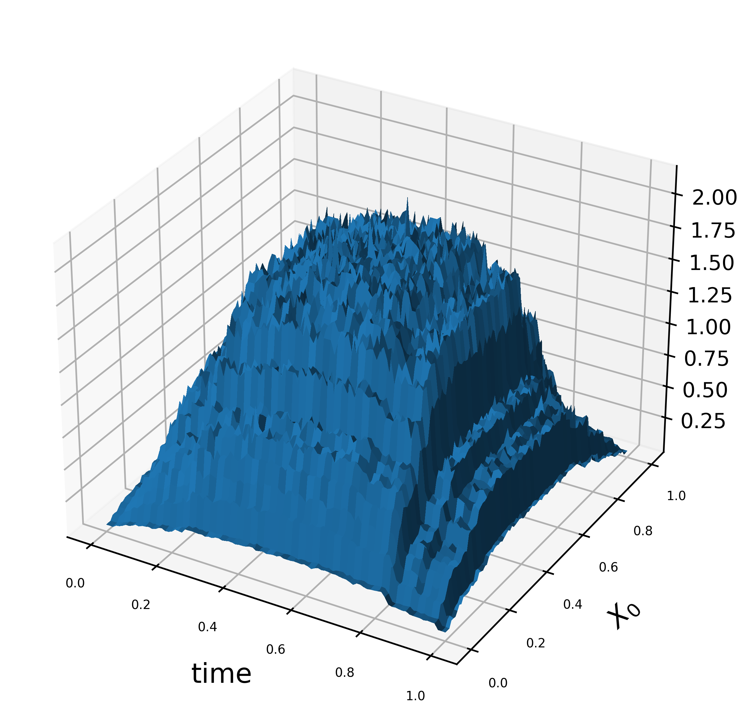
Figure 1: The estimated hazard values as a function of time and one of the covariates, $X_{0}$.

4.7 Survivor curve estimation for time-static covariates

Recall from Section 1 that the survivor curve $S(t|X)=\mathbb{P}(T>t|X)$ is not meaningful when the covariates $X(t)$ change over time. However, for time-static covariates $X(t)=X$, $S(t|X)$ can be obtained from the estimated hazard function.

As an example, suppose we want to obtain the survivor curve conditional on the covariate vector $(X_{0}=0.20202,\cdots,X_{10}=0.128217)$. We wish to evaluate the curve at $t=0,0.01,0.02,\cdots,0.99$. We use the code below to generate the pandas dataframe: t = [t/100 for t in range(0, 100)] df_surv = pd.concat([test_X.loc[2000].to_frame().T]*len(t)) df_surv = df_surv.reset_index(drop=True) df_surv[’t’] = t

t X_0 … X_10 0 0.00 0.20202 0.128217 1 0.01 0.20202 0.128217 2 0.02 0.20202 0.128217 .. … … … 98 0.98 0.20202 0.128217 99 0.99 0.20202 0.128217

To estimate the value of the survivor curve for each row, run:

surv_vals = boxhed_.survivor(df