Anisotropic relativistic fluid spheres with a linear equation of state

Abstract

In this work, we present a class of relativistic and well-behaved solution to Einstein’s field equations for anisotropic matter distribution. We perform our analysis by using the Buchdahl ansatz for the metric function $g_{rr}$. Three different classes of new exact solution are found for anisotropy factor $\Delta$. We have analyzed our model with various physical aspects such as pressure (radial as well as transverse), energy density, anisotropy factor, mass, compactness parameter, adiabatic index $\gamma$ and surface redshift. A graphical analysis of energy conditions, TOV equation and causality condition indicates the model are well behaved. The physical acceptability of the model has verified by considering compact objects with similar mass and radii, such as 4U 1820-30,Vela X-1, PSR J1614-2230, LMC X-4, SMC X-1, 4U 1538-52, Her X-1, Cgy X-2, PSR B1913+16 and PSR J1903+327.

1 Introduction

Due to the highly nonlinear behavior of Einstein’s field equations, one of the most important problems in General Relativity is to obtain exact solution of Einstein equations. Exact solution play important role in the development of many areas of gravitational significance such as the study of effects of gravitation in solar system, black hole,star,gravitational collapse,cosmology and dynamic of early universe. Schwarzschild [1], Tolman [2] and Oppenheimer and Volkoff [3] have deal with self-gravitating isotropic fluid spheres, set up two approaches that can be followed in order to solve the field equations. The first one consists in making a suitable assumption of the metric functions or energy density. This leads to the finding unknown variables, which are the isotropic pressure and the other metric potential. However, in the framework of this method not always is possible to obtain an exact solution (sometimes one obtains nonphysical pressure-density configurations). The second approach deal with an equation of state which is integrated (iteratively from the center of the compact object) until the pressure vanished indicating that the object surface has been reached. As before, this scheme also presents some drawbacks since it does not always lead to a closed form of the solutions. Many projects are suggested by Ivanov[4] for constructing charged fluid spheres. The perfect fluid solution was found Gupta and Kumar[5].

On the other hand, a stellar configuration sometimes have not followed the isotropic condition at all (equal radial $p_{r}$ and tangential $p_{t}$ pressure). In fact, the theoretical studies by Canuto [6, 7, 8], Canuto et. al [9, 10, 11] and Ruderman [12], observed that when the matter density is higher than the nuclear density, it may be anisotropic in nature and must be treated relativistically. So, rest the isotropic condition and allow the presence of anisotropy (it leads to unequal radial and tangential pressure $p_{r}\neq p_{t}$ ) within the stellar configuration represent a more realistic situation in the astrophysical sense. Furthermore, the pioneering contribution to local anisotropic properties by Bowers and Liang’s [13] for static spherically symmetric and relativistic configurations, gave rise an extensive studies within this framework, specifically studies focused on the dynamical incidence of the anisotropies in the arena of equilibrium and stability on collapsed structures [14, 15, 16]. Moreover, as Mak and Harko have contended [17], anisotropy can merge in various settings such as: the presence of a strong center or by the existence of type 3A superfluid [18], pion condensation [19] or various types of regime transitions[20].

In different circumstance, the spherical symmetry also allows a more general anisotropic fluid configuration with an equation of state(EoS). If one knows the EoS of the material composition of a compact star, then one can easily integrate the Tolman-Oppenheimer-Volkoff (TOV) equations to extract the geometrical information of the compact star. For example, Ivanov [4] used a linear EoS for charged static spherically symmetric perfect fluid solutions. Sharma and Maharaj [21] have been extended this condition for finding an exact solution to the Einstein field equations with an anisotropic matter distribution. Herrera and Barreto [22] had considered polytropic stars with anisotropic pressure. Many solutions [23, 24, 25, 26, 27, 28] of Einstein’s equations have been found for anisotropic fluid distribution with different EoS, but, in case the EoS of the material composition of a compact star is not yet known, except some phenomenological assumptions, for example, one can introduce a suitable metric ansatz for one of the metric functions to analyze the physical features of the star. Initially, this type of method was proposed by Vaidya-Tikekar [29], and Tikekar [30] introduced an approach of assigning different geometries with physical 3-spaces (see [31, 32, 33, 5] and references therein). Finch and Skea [34] have also considered such type of metric ansatz that satisfying all criteria of physical acceptability according to Delgaty and Lake [35]. This type of the problem in which to finding the equilibrium configuration of a stellar structure for anisotropic fluid distribution has been found in [36, 37, 38, 39] . Moreover, our stellar model incorporates a family of new solutions for a static spherically symmetric anisotropic fluid structure with the help of Buchdahl metric potential. In this paper, we consider analogue objects with similar mass and radii, such as PSR J1614-2230 [40] 4U 1538-52 [41], LMC X-4 [42], SMC X-1 [41], Her X-1 [43], Vela X-1 [41], PSR J1903+327 [44], PSR B1913+ 16 [45], 4U 1820-30 [46], Cyg X-1 [47].

The remainder of the article is arranged as follows: Section 2 presents the Einstein’s field equations for anisotropic matter distributions and the approach followed in order to solve them, in section 4 we match the obtained model with the exterior spacetime given by Schwarzschild metric, in order to obtain the constant parameters. In section 5 we analyze the causality condition. Section 6 is devoted to the study of the equilibrium via Tolman-Oppenheimer-Volkoff (TOV) equation. Sections 7 and 9 describe adiabatic index and conclusion respectively.

2 Field Equation

Let us consider the static spherically symmetric metric in Schwarzschild coordinates

$$ds^{2}=-e^{\lambda(r)}dr^{2}-r^{2}(d\theta^{2}+\sin^{2}\theta d\phi^{2})+e^{\nu(r)}dt^{2}$$ (1)

where $\lambda(r)$ and $\nu(r)$ are the functions of radial coordinate $r.$ If (1) describes anisotropic matter distribution then the space-time(1) has to satisfy satisfy the energy-momentum tensor

$$T^{i}_{j}=(\rho+p_{t})u^{i}u_{j}-p_{t}\delta^{i}_{j}+(p_{r}-p_{t})\chi^{i}\chi_{j}$$ (2)

with $u^{i}u_{j}=-\chi^{i}\chi_{j}=1$, where $\nu^{i},\chi^{i},\rho,p,p_{t}$ are the fluid four velocity,unit space-like vector, energy density, radial and transverse pressures respectively. Thus, the Einstein field equation for line element(1) with respect to energy-momentum tensor(2) reduce to (Landau and Lifshitz[48])

$$\kappa p_{r} = \dfrac{\nu^{\prime}}{r}e^{-\lambda}-\dfrac{(1-e^{-\lambda})}{r^{2}}$$ (3)

$$\kappa p_{t} = \bigg{(}\dfrac{\nu^{\prime\prime}}{2}-\dfrac{\lambda^{\prime}\nu^{\prime}}{4}+\dfrac{\nu^{{}^{\prime}2}}{4}+\dfrac{\nu^{\prime}-\lambda^{\prime}}{2r}\bigg{)}e^{-\lambda}$$ (4)

$$\kappa\rho = \dfrac{\lambda^{\prime}}{r}e^{-\lambda}+\dfrac{(1-e^{-\lambda})}{r^{2}}$$ (5)

where $\kappa=8\pi$ and the prime denotes the derivative with respect to $r$. Here we will work on $c=G=1$, where $c$ is the speed of light and $G$ is the gravitational constant.Consequently, $\Delta=p_{t}-p_{r}$ is denoted as the anisotropy factor according to Herrera and Leon [49],and it measures the pressure anisotropy of the fluid. It is to be noted that at the origin of the stellar configuration $\Delta=0$, i.e., $p_{t}=p_{r}$ is a particular case of an isotropic pressure. Using eqs.(3) and (4), one can obtain the simple form of anisotropic factor($\Delta=0$) , which yields

$$\Delta=\kappa\,(p_{t}-\,p_{r})=e^{-\lambda}\left[\frac{\nu^{\prime\prime}}{2}-\frac{\lambda^{\prime}\nu^{\prime}}{4}+\frac{{\nu^{\prime}}^{2}}{4}-\frac{\nu^{\prime}+\lambda^{\prime}}{2r}-\frac{1}{r^{2}}\right]\,+\frac{1}{r^{2}}.$$ (6)

The anisotropic pressure is repulsive if $p_{t}>p_{r}$ and attractive if $p_{t}<p_{r}$ of the stellar model.In the system of equs.(3)-(5), we have three equations with five unknowns.Thus, the system of equations is undetermined. Hence,to solve these equation we have to reduce the number of unknown functions.

3 Exact Solution of the Model for Anisotropic Stars

In this section we solve the system of equs.(3)-(5). For this we employ a well known metric ansatz[50] that encompasses almost all the known solutions to the static Einstein equations with a perfect fluid source which is given by

$$e^{\lambda}=\frac{K\,(1+Cr^{2})}{K+Cr^{2}},~{}~{}~{}~{}~{}\textrm{with}~{}~{}~{}K<0~{}~{}~{}\textrm{and}~{}~{}C>0,$$ (7)

where $K$ and $C$ are constant parameters that characterize the geometry of the star. Initially the Buchdahl[50] have considered above metric potential to study a relativistic compact star. Note that above metric potential is free from singularity at $r=0$ and the metric coefficient is $e^{\lambda(0)}=1.$ Moreover it provides a monotonic decreasing energy density as follows

$$\frac{\kappa\rho}{C}=\dfrac{(K-1)(3+Cr^{2})}{K(1+Cr^{2})^{2}}$$ (8)

Now we introduce the transformation $e^{\nu}=Z^{2}(r)$ and substituting the value of $e^{\lambda}$ in equ.(6), we get

$$\frac{d^{2}Z}{dr^{2}}-\left[\frac{K+2\,K\,Cr^{2}+C^{2}r^{4}}{r\,(K+Cr^{2})\,(1+Cr^{2})}\right]\,\frac{dZ}{dr}+\left[\frac{(1-K)\,C^{2}r^{4}}{r^{2}\,(K+Cr^{2})\,(1+Cr^{2})}-\frac{\Delta~{}K\,(1+Cr^{2})}{(K+Cr^{2})}\,\right]\,Z=0.$$ (9)

In order to solve equ.(9) for $Z$, we will use Mak and Harko’s approach[17]. Therefore we are taking an appropriate transformation $X=\sqrt{\dfrac{K+Cr^{2}}{K-1}}$ and $Z=(1-X^{2})^{1/4}\,Y$, equ.(9) transform to a differential equation of the form

$$\frac{d^{2}Y}{dX^{2}}+\frac{1}{(1-X^{2})}\Bigg{[}1-K+\frac{\Delta\,K(K-1)^{2}\,(X^{2}-1)^{2}}{((K-1)\,(X^{2}-1)-1)^{2}}-\frac{2+3X^{2}}{4(1-X^{2})}\Bigg{]}Y=0$$ (10)

Here, our aim is to solve the equ.(10) by using Bijalwan and gupta’s approach[51].In this framework, we choose the expression for anisotropy

$$\Delta=C^{2}r^{2}\Big{[}\frac{(1-K)(4K\,Cr^{2}-7\,Cr^{2}-K-2)+\alpha(1+Cr^{2})^{2}}{4K(1-K)(1+Cr^{2})^{3}}\Big{]}$$ (11)

where $\alpha$ is an arbitrary constant that can take positive, negative or zero value.In equ.(11), $\Delta=0$ at the center ,i.e. the radial pressure is equal to the tangential pressure at the center.Now using the value of $\Delta$ in equ.(10),we have

$$\frac{d^{2}Y}{dX^{2}}+\alpha Y=0$$ (12)

which is a second order differential equation in Y. Now, we are classifying each solution of equation(12), briefly

$$\textrm{Case~{} I:}~{}~{}~{}Y =A_{1}\,X+B_{1},~{}~{}~{}~{}~{}~{}~{}~{}~{}~{}~{}~{}~{}~{}~{}\textrm{if}~{}~{}~{}\alpha=0$$ (13a)

$$\textrm{Case~{} II:}~{}~{}~{}Y =A_{2}\,e^{\Phi\,X}+B_{2}\,e^{-\Phi\,X},~{}~{}~{}~{}~{}~{}~{}~{}~{}~{}~{}~{}~{}\textrm{if}~{}~{}~{}\alpha=-\Phi^{2}$$ (13b)

$$\textrm{Case~{} III:}~{}~{}~{}Y =A_{3}\,\cos(\Phi\,X)+B_{3}\,\sin(\Phi\,X),~{}~{}~{}~{}~{}~{}~{}~{}~{}~{}\textrm{if}~{}~{}~{}\alpha=\Phi^{2}$$ (13c)

where $A_{1}$, $B_{1}$, $A_{2}$, $B_{2}$, $A_{3}$, and $B_{3}$ are arbitrary constant of integration.Now the expression of radial and tangential pressure can be derived as follows in original coordinates,
Case I:

$$Z(r) = A_{1}\Bigg{(}\frac{1+Cr^{2}}{1-K}\Bigg{)}^{1/4}\Bigg{(}\sqrt{\frac{K+Cr^{2}}{K-1}}+\frac{B_{1}}{A_{1}}\Bigg{)}$$ (14)

$$\frac{\kappa p_{r}}{C} = \frac{K+Cr^{2}}{K(1+Cr^{2})^{2}}+\frac{2\sqrt{K+Cr^{2}}}{K(1+Cr^{2})(\sqrt{K+Cr^{2}}+B_{1}/A_{1}\sqrt{K-1})}+\frac{1-K}{K(1+Cr^{2})}$$ (15)

$$\frac{\kappa p_{t}}{C} = \frac{K+Cr^{2}}{K(1+Cr^{2})^{2}}+\frac{2\sqrt{K+Cr^{2}}}{K(1+Cr^{2})(\sqrt{K+Cr^{2}}+(B_{1}/A_{1})\sqrt{K-1})}+\frac{1-K}{K(1+Cr^{2})}+\Delta_{1}$$ (16)

$$\textrm{where}~{}~{}~{}~{}\Delta_{1} = \frac{Cr^{2}}{4K(1+Cr^{2})^{3}}\Big{[}4K\,Cr^{2}-7\,Cr^{2}-K-2\Big{]}$$

Case II:

$$Z(r) = A_{2}\Bigg{(}\frac{1+Cr^{2}}{1-K}\Bigg{)}^{1/4}\Bigg{(}e^{\Phi\sqrt{\frac{K+Cr^{2}}{K-1}}}+(B_{2}/A_{2})\,e^{-\Phi\sqrt{\frac{K+Cr^{2}}{K-1}}}\Bigg{)}$$ (17)

$$\frac{\kappa p_{r}}{C} = \frac{K+Cr^{2}}{K(1+Cr^{2})^{2}}+\frac{2\sqrt{K+Cr^{2}}}{K\sqrt{K-1}(1+Cr^{2})}\left(\frac{e^{\Phi\sqrt{\frac{K+Cr^{2}}{K-1}}}-(B_{2}/A_{2})\,e^{-\Phi\sqrt{\frac{K+Cr^{2}}{K-1}}}}{e^{\Phi\sqrt{\frac{K+Cr^{2}}{K-1}}}+(B_{2}/A_{2})\,e^{-\Phi\sqrt{\frac{K+Cr^{2}}{K-1}}}}\right)+\frac{1-K}{K(1+Cr^{2})}$$ (18)

$$\frac{\kappa p_{t}}{C} = \frac{K+Cr^{2}}{K(1+Cr^{2})^{2}}+\frac{2\sqrt{K+Cr^{2}}}{K\sqrt{K-1}(1+Cr^{2})}\left(\frac{e^{\Phi\sqrt{\frac{K+Cr^{2}}{K-1}}}-(B_{2}/A_{2})\,e^{-\Phi\sqrt{\frac{K+Cr^{2}}{K-1}}}}{e^{\Phi\sqrt{\frac{K+Cr^{2}}{K-1}}}+(B_{2}/A_{2})\,e^{-\Phi\sqrt{\frac{K+Cr^{2}}{K-1}}}}\right)+\frac{1-K}{K(1+Cr^{2})}+\Delta_{2}$$

$$\textrm{where}~{}~{}~{}~{}\Delta_{2} = \frac{Cr^{2}}{K(1+Cr^{2})^{2}}\Bigg{[}\frac{4K\,Cr^{2}-7\,Cr^{2}-K-2}{4(1+Cr^{2})}-\frac{\Phi(1+Cr^{2})}{1-K}\Bigg{]}$$

Case III:

$$Z(r) = A_{3}\Bigg{(}\frac{1+Cr^{2}}{1-K}\Bigg{)}^{1/4}\Bigg{[}\cos\Big{(}\Phi\sqrt{\frac{K+Cr^{2}}{K-1}}\Big{)}+(B_{3}/A_{3})\,\sin\Big{(}\Phi\sqrt{\frac{K+Cr^{2}}{K-1}}\Big{)}\Bigg{]}$$ (20)

$$\frac{\kappa p_{r}}{C} = \frac{K+Cr^{2}}{K(1-K)(1+Cr^{2})}\left[\frac{1-K}{1+Cr^{2}}-2\Phi\sqrt{\frac{K-1}{K+Cr^{2}}}F(r)\right]+\frac{1-K}{K(1+Cr^{2})}$$ (21)

$$\frac{\kappa p_{r}}{C} = \frac{K+Cr^{2}}{K(1-K)(1+Cr^{2})}\left[\frac{1-K}{1+Cr^{2}}-2\Phi\sqrt{\frac{K-1}{K+Cr^{2}}}F(r)\right]+\frac{1-K}{K(1+Cr^{2})}+\Delta_{3}$$ (22)

$$\textrm{where}~{}~{}~{}~{}\Delta_{3} = \frac{Cr^{2}}{K(1+Cr^{2})^{2}}\Bigg{[}\frac{4K\,Cr^{2}-7\,Cr^{2}-K-2}{4(1+Cr^{2})}+\frac{\Phi(1+Cr^{2})}{1-K}\Bigg{]}$$

$$F(r) = \left(\frac{(B_{3}/A_{3})\,\cos\Big{(}\Phi\sqrt{\frac{K+Cr^{2}}{K-1}}\Big{)}-\sin\Big{(}\Phi\sqrt{\frac{K+Cr^{2}}{K-1}}\Big{)}}{\cos\Big{(}\Phi\sqrt{\frac{K+Cr^{2}}{K-1}}\Big{)}+(B_{3}/A_{3})\,\sin\Big{(}\Phi\sqrt{\frac{K+Cr^{2}}{K-1}}\Big{)}}\right)$$

In a realistic scenario, the following physical character of above solutions is required:

1. the energy density is positive definite and decreasing monotonically within $0<r<R,$ i.e., its gradient is negative within $0<r<R.$

2. the pressure is positive definite and decreasing monotonically within $0<r<R,$ i.e., its gradient is negative within $0<r<R.$

3. the ratio of pressure and energy density is less than unity within the stellar model.

4. the radial pressure should be vanished at the boundary but the tangential pressure needs not necessarily vanish. However, the radial pressure is equal to the tangential pressure at the center, i.e, $\Delta(0)=0$[4, 13].

To examine the positive density and pressure of realistic star, we plot this in Fig.(1). In Fig.(2), we can show that the anisotropy($\Delta$) vanishes at the center and increasing monotonically within stellar model which implies tangential pressure is always greater than radial pressure. Also ratio of pressure and density, i.e, $\frac{p_{r}}{\rho}$ and $\frac{p_{t}}{\rho}$ lie between $0$ to $1$, which state that the underlying fluid distribution is real and nonexotic in nature [52].

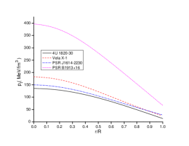
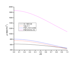
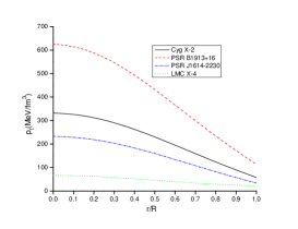
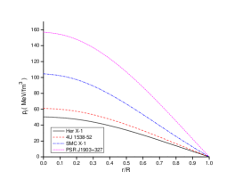
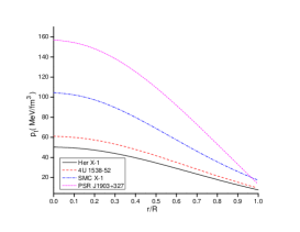
Figure 1: Behaviour of radial pressure, tangential pressure and density vs. fractional radius $r/R$ for case I(first row), case II(second row) and case III(third row). The values of the parameter which we have used for graphical presentation are:(i) $K=-0.4995,~{}C=0.0023km^{-2}$ for 4U 1820-30 (case I) ; (ii) K = -1.097, $C=0.0044km^{-2}$ for Vela X-1 (case I); (iii) K = -0.901, $C=0.0042km^{-2}$ for PSR J1614-2230 (case I); (iv) K = -0.798, $C=0.0092km^{-2}$ for PSR B1913+16 (case I); (v) K = -.8196, $C=0.0055km^{-2},\,\,\alpha=-0.64$ for Cgy X-2 (case II); (vi) K =-0.82, $C=0.0094km^{-2},\,\,\,\alpha=-0.81$ for PSR B1913+16 (case II); (vii) K = -0.8202, $C=0.0039km^{-2},\,\,\,\alpha=-0.36$ for PAR J1614-2230 (case II); (viii) K = -2.977, $C=0.0055km^{-2},\,\,\,\alpha=-2.25$ for LMC X-4 1937+21 (case II); (ix) K=-1.9779, $C=0.0039km^{-2},\,\,\,\alpha=0.0081$ for Her X-1 (case III); (x) K=-1.9779, $C=0.0045km^{-2},\,\,\,\alpha=0.0064$ for 4U1538-52 (case III); (xi) K=-1.9776, $C=0.0052km^{-2},\,\,\,\alpha=0.0049$ for SMC X-1 (case III); (xii) K=-0.6, $C=0.0027km^{-2},\,\,\,\alpha=0.16$ for PSR J1903+327 (case III).See Table 1 for more details

Figure 2: Behaviour of anisotropic factor and pressure-density ratio vs. fractional radius $r/R$ for case I(first row), case II(second row) and case III(third row).For plotting this figure we have employed data set values of physical parameters and constants which are the same as used in Fig.1.

4 Boundary condition

In order to find the arbitrary constant $A_{1}$, $B_{1}$, $A_{2}$, $B_{2}$, $A_{3}$, and $B_{3}$ we match our interior spacetime(1) to the exterior Schwarzschild line element at the boundary of the star($r=R$). The expression of exterior Schwarzschild line element is as follows

$$ds^{2}=-\bigg{(}1-\frac{2M}{r}\bigg{)}^{-1}dr^{2}-r^{2}(d\theta^{2}+\sin^{2}\theta d\phi^{2})+\bigg{(}1-\frac{2M}{r}\bigg{)}dt^{2}$$ (23)

where $M$ is the gravitational mass of the distribution such that

$$M(r)=\dfrac{\kappa}{2}\int_{0}^{r}\rho r^{2}dr,$$

Using the Darmois-Israel boundary condition[53], we match line elements (1) and (23) at the boundary ($r=R$) which are tantamount to the following two conditions

$$e^{-\lambda}=1-\dfrac{2M}{R},~{}~{}~{}\textrm{and}~{}~{}~{}e^{\nu}=y^{2}=1-\dfrac{2M}{R}$$ (24)

$$p_{r}(R)=0.$$ (25)

Now using the conditions (24) and (25), we can compute the values of arbitrary constants. Thus the expression of arbitrary constants $A_{1}$ to $A_{3}$ and $B_{1}$ to $B_{3}$ as follows:

$$\frac{B_{1}}{A_{1}} = -\sqrt{\frac{K+CR^{2}}{K-1}}\Bigg{[}1+\frac{2(1+CR^{2})}{2\,CR^{2}+1-K\,CR^{2}}\Bigg{]}$$

$$\frac{B_{2}}{A_{2}} = \Bigg{[}\frac{2\,CR^{2}+1-K\,CR^{2}+2\Phi\sqrt{\frac{K+CR^{2}}{K-1}}}{2\Phi\sqrt{\frac{K+CR^{2}}{K-1}}-2\,CR^{2}-1+K\,CR^{2}}\Bigg{]}e^{\Big{(}\Phi\sqrt{\frac{K+Cr^{2}}{K-1}}\Big{)}}$$

$$\frac{B_{3}}{A_{3}} = \frac{G(R)\cos\Big{(}\Phi\sqrt{\frac{K+CR^{2}}{K-1}}\Big{)}+G_{1}(R)\sin\Big{(}\Phi\sqrt{\frac{K+CR^{2}}{K-1}}\Big{)}}{G_{1}(R)\sin\Big{(}\Phi\sqrt{\frac{K+CR^{2}}{K-1}}\Big{)}-G(R)\cos\Big{(}\Phi\sqrt{\frac{K+CR^{2}}{K-1}}\Big{)}}$$

$$\textrm{where}~{}~{}~{}G(R) = \frac{2\,CR^{2}+1-K\,CR^{2}}{K(1+CR^{2})^{2}},~{}~{}~{}~{}~{}~{}G_{1}(R)=\frac{2\Phi(K+CR^{2})}{K(K-1)(1+CR^{2})}\sqrt{\frac{K-1}{K+CR^{2}}}$$

One can decide the absolute mass M of the star for a given radius R. It might be referenced here that limits on excellent structures, including the mass-radius ratio as proposed by the Buchdahl-Bondi condition[50, 54], exist and are given by $\frac{2M}{R}\leq\frac{8}{9}$. This fills in as an upper bound on the absolute compactness of the static spherically symmetric isotropic compact stars. However, this bound has been refreshed in the presence of charged gravitational fields[55, 56], for a nonzero cosmological constant[57] and use of the thin-shell formalism[58]. The effect of the mass-radius ratio on the equation of state has been considered by Carvalho et al. [59] for white dwarf and neutron stars and for the nuclear center by Lattimer[60]. Here, we have find specific masses and radii(see in Table-1) of the compact star estimated by Gangopadhyay et al.[61].

The gravitational redshift from the surface of the star as measured by a distant observer $(g_{tt}\rightarrow-1)$ is given by

$$z_{s}=e^{\lambda(R)}-1=\dfrac{1-\sqrt{1-\frac{2M}{R}}}{\sqrt{1-\frac{2M}{R}}}$$

where $g_{tt}(R)=e^{\nu(R)}=(1-\frac{2M}{R})$ is the metric function. Buchdahl[50] have observed that the gravitational redshift is $z_{s}<2$ for spherically symmetric distribution of a prefect fluid. However, Karmakar and Barraco [62, 63] suggested that the gravitational redshift of anisotropy star models is 3.84. Therefore, the resulting surface redshift (see Fig.7) from the solution also compatible with this discussion.

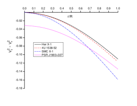
Figure 3: Behaviour of speed of sound vs. fractional radius $r/R$ for case I(first row), case II(second row) and case III(third row). For plotting this figure we have employed data set values of physical parameters and constants which are the same as used in Fig.1.

5 Mass function and Compactness

In this section, we have discussed the mass function $M(r)$ and mass-radius relationship i.e, compactness parameter $u(r)$. Buchdahl[50] suggested that the mass-radius ratio of a relativistic static spherically symmetric fluid stellar model should be $\frac{M}{R}\leq\frac{4}{9}$. In this context, Mak and Harko [17] have obtained a generalized formula for the mass-radius ratio. In our model, we have obtained the mass function and compactness parameter of relativistic compact stars as follows

Figure 4: Behaviour of mass function and compactness parameter vs. fractional radius $r/R$ for case I(first row), case II(second row) and case III(third row). For plotting this figure we have employed data set values of physical parameters and constants which are the same as used in Fig.1.

$$M(r)=\dfrac{Cr^{3}(K-1)}{2K\,(1+Cr^{2})},$$ (26)

$$u=\dfrac{M}{r}=\dfrac{Cr^{2}(K-1)}{2K\,(1+Cr^{2})}$$ (27)

Through compactness parameter, we can analyze many extreme properties to compact objects, such as, the emission of x-rays and gamma-rays, which makes them relevant for the high energy astrophysics. The profile of $M(r)$ and $u(r)$ has shown in Fig.4. we can see that the mass function is regular at the center of the stars. Also it is monotonic increasing function of $r$ and positive inside the relativistic compact stars and the compactness parameter $u(r)$ increases with increase $r/R$. This shows that the compactness of compact stars lies in the expected range of Buchdahl limit[50]. We have calculated this bound for compact stars in our model and have shown it in Table 1.

6 Causality condition and Herrera’s cracking method

For any relativistic star, radial and transverse velocity of sound should satisfy $v_{r}^{2},v_{t}^{2}\leq 1$ and this is known as the causality condition. On the other hand, Le Chatelier’s principle demands that the speed of sound be positive, i.e.,$v_{r}^{2},v_{t}^{2}\geq 0$. Combining the above two inequalities, one gets $0<v_{r}^{2},v_{t}^{2}\leq 1$, where the radial and transverse velocity of sound are obtained as

$$v_{r}^{2}=\frac{dp_{r}}{d\rho}=\frac{dp_{r}}{dr}/\frac{d\rho}{dr}$$ (28)

$$v_{t}^{2}=\frac{dp_{t}}{d\rho}=\frac{dp_{t}}{dr}/\frac{d\rho}{dr}$$ (29)

where $\dfrac{d\rho}{dr}=\dfrac{2Cr\,(1-K)(5+Cr^{2})}{K(1+Cr^{2})^{3}}$, the expressions of $=\frac{dp_{r}}{dr}~{}~{}\textrm{and}~{}~{}\frac{d\rho}{dr}$ are as follows
Case I

$$\frac{dp_{r}}{dr} = \frac{2Cr}{K}\left[\frac{K(Cr^{2}-1)-2Cr^{2}}{\left(1+Cr^{2}\right)^{3}}+\frac{1+Cr^{2}}{\sqrt{K+Cr^{2}}}-2\sqrt{K+Cr^{2}}-\frac{\left(1+Cr^{2}\right)}{(\sqrt{K+Cr^{2}}+(B_{1}/A_{1})\sqrt{K-1})}\right]$$ (30)

$$\frac{dp_{t}}{dr} = \frac{dp_{r}}{dr}+\frac{Cr}{2K(1+Cr^{2})^{3}}\left[(4K-7)Cr^{2}+\frac{1-2Cr^{2}(4KCr^{2}-7Cr^{2}-K-2)}{1+Cr^{2}}\right]$$ (31)

Case II

$$\frac{dp_{r}}{dr} = \frac{2Cr}{K}\Bigg{[}\frac{K(Cr^{2}-1)-2Cr^{2}}{\left(1+Cr^{2}\right)^{3}}+\frac{\Phi\left(1-2K-Cr^{2}\right)}{\sqrt{K-1}\sqrt{K+Cr^{2}}\left(1+Cr^{2}\right)^{2}}\left(\frac{e^{\Phi\sqrt{\frac{K+Cr^{2}}{K-1}}}-(B_{2}/A_{2})\,e^{-\Phi\sqrt{\frac{K+Cr^{2}}{K-1}}}}{e^{\Phi\sqrt{\frac{K+Cr^{2}}{K-1}}}+(B_{2}/A_{2})\,e^{-\Phi\sqrt{\frac{K+Cr^{2}}{K-1}}}}\right)$$ (32)

$$+\frac{4\Phi^{2}(B_{2}/A_{2})}{(K-1)(1+Cr^{2})\Big{(}e^{\Phi\sqrt{\frac{K+Cr^{2}}{K-1}}}+(B_{2}/A_{2})\,e^{-\Phi\sqrt{\frac{K+Cr^{2}}{K-1}}}\Big{)}}\Bigg{]}$$

$$\frac{dp_{t}}{dr} = \frac{dp_{r}}{dr}+\frac{2Cr}{K(1+Cr^{2})^{2}}\left[\frac{(K-1)5Cr^{2}}{4(1+Cr^{2})^{2}}+\frac{1-2Cr^{2}(4KCr^{2}-7Cr^{2}-K-2)}{4(1+Cr^{2})}-\frac{\Phi^{2}(1+Cr^{2})}{1-K}\right]$$ (33)

Case III

$$\frac{dp_{r}}{dr} = \frac{2Cr}{K}\Bigg{[}\frac{K(Cr^{2}-1)-2Cr^{2}}{\left(1+Cr^{2}\right)^{3}}+\frac{\Phi\left(1-2K-Cr^{2}\right)}{\sqrt{K-1}\sqrt{K+Cr^{2}}\left(1+Cr^{2}\right)^{2}}F(r)$$ (34)

$$+\frac{-\Phi^{2}(1+(B_{3}/A_{3})^{2})}{(K-1)(1+Cr^{2})\Big{(}\cos\Big{(}\Phi\sqrt{\frac{K+Cr^{2}}{K-1}}\Big{)}+(B_{3}/A_{3})\,\sin\Big{(}\Phi\sqrt{\frac{K+Cr^{2}}{K-1}}\Big{)}\Big{)}}\Bigg{]}$$

$$\frac{dp_{t}}{dr} = \frac{dp_{r}}{dr}+\frac{2Cr}{K(1+Cr^{2})^{2}}\left[\frac{(K-1)5Cr^{2}}{4(1+Cr^{2})^{2}}+\frac{1-2Cr^{2}(4KCr^{2}-7Cr^{2}-K-2)}{4(1+Cr^{2})}+\frac{\Phi^{2}(1+Cr^{2})}{1-K}\right]$$ (35)

With the help of graphical representation we have shown that our model satisfies the causality condition (please see Fig.3(left)). Now we are interested in checking the stability of the anisotropic stars under the radial perturbations using the concept of Herrera[64]. By using the principle of Herrera [64], Abreu et al.[65] introduced the concept of ”cracking”, which states that the region of an anisotropic fluid sphere, where $-1\leq v_{t}^{2}-v_{r}^{2}\leq 0$, is potentially stable but the region where $0<v_{t}^{2}-v_{r}^{2}\leq 1$ is potentially unstable. From Fig.3(right) it is clear that our model is potentially stable. Moreover $0<v_{r}^{2}<1$ and $0<v_{r}^{2}<1$ therefore, according to Andreasson[56], $|v_{r}^{2}-v_{t}^{2}|<1$ which is also shown in Fig.3(left).

7 Tolman-Oppenheimer-Volkoff (TOV) equations

Now we are interested in checking the effect of three different forces, viz. gravitational, hydrostatic and anisotropic force,on our given system. The governing generalized Tolman-Oppenheimer-Volkoff(TOV) equation [2, 3] is given by

$$-\frac{M_{G}(\rho+p_{r})}{r^{2}}e^{\frac{\lambda-\nu}{2}}-\frac{dp_{r}}{dr}+\frac{2(p_{t}-p_{r})}{r}=0,$$ (36)

where $M_{G}$ is the effective gravitational mass given by:

$$M_{G}(r)=\frac{1}{2}r^{2}\nu^{\prime}e^{(\nu-\lambda)/2}.$$ (37)

From the equation(37) the value of $M_{G}(r)$ in equation (36), we get

$$-\frac{\nu^{\prime}}{2}(\rho+p_{r})-\frac{dp_{r}}{dr}+\frac{2(p_{t}-p_{r})}{r}=0,$$ (38)

The equation (38) can be expressed into three different elements gravitational $(F_{g})$, hydrostatic $(F_{h})$ and anisotropic force $(F_{a})$ from an equilibrium point of view, which are defined as:

$$F_{g}=-\frac{\nu^{\prime}}{2}(\rho+p),~{}~{}~{}~{}F_{h}=-\frac{dp_{r}}{dr}~{}~{}~{}~{}\textrm{and}~{}~{}~{}~{}F_{a}=\frac{2(p_{t}-p_{r})}{r}=\frac{2\Delta}{C}$$ (39)

Here, we can derive the hydrostatic force $(F_{h})$ from eqns.(30),(32), (34) and anisotropic force $(F_{a})=\Delta_{i}$, where $i=1,2,3$ for case I, case II and case III. Now the expression of gravitational force $F_{g}$ is written in an explicit form:
Case I

$$F_{g}=\frac{Cr}{1-K}\left[\frac{1-K}{2(1+Cr^{2})}-\frac{\sqrt{\frac{K-1}{K+Cr^{2}}}}{\sqrt{\frac{K+Cr^{2}}{K-1}}+(B_{1}/A_{1})}\right]$$ (40)

Case II

$$F_{g}=\frac{Cr}{1-K}\left[\frac{1-K}{2(1+Cr^{2})}-\Phi\sqrt{\frac{K-1}{K+Cr^{2}}}\left(\frac{e^{\Phi\sqrt{\frac{K+Cr^{2}}{K-1}}}-(B_{2}/A_{2})\,e^{-\Phi\sqrt{\frac{K+Cr^{2}}{K-1}}}}{e^{\Phi\sqrt{\frac{K+Cr^{2}}{K-1}}}+(B_{2}/A_{2})\,e^{-\Phi\sqrt{\frac{K+Cr^{2}}{K-1}}}}\right)\right]$$ (41)

Case III

$$F_{g}=\frac{Cr}{1-K}\left[\frac{1-K}{2(1+Cr^{2})}-\Phi\sqrt{\frac{K-1}{K+Cr^{2}}}F(r)\right]$$ (42)

Figure (5) represents the behavior of the generalized TOV equations. We observe from these figures that the system is counterbalanced by the components the gravitational force $(F_{g})$, hydrostatic force$(F_{h})$ and electric force $(F_{e})$ and the system attains a static equilibrium.

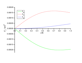
Figure 5: Behaviour of hydrostatic, anisotropic and gravitational forces vs. fractional radius $r/R$ for case I(first four graph), case II(middle four graph) and case III(last four graph).For plotting this figure we have employed data set values of physical parameters and constants which are the same as used in Fig.1.

8 Energy conditions

Inside the anisotropic matter distribution, we analyze the energy conditions according to relativistic classical field theories of gravitation. In the context of GR the energy conditions should be positive. Here we will focus on (i) the null energy condition (NEC), (ii) the weak energy condition (WEC), and (iii) the strong energy condition (SEC)[66, 67]. In summary:

1. (NEC) $\rho\geq 0$

2. (WECr) $\rho-p_{r}\geq 0$

3. (NECt) $\rho-p_{t}\geq 0$

4. (SEC) $\rho-p_{r}-2p_{t}\geq 0$

Figure (6)demonstrated that all the above inequalities are fulfilled inside the spherical object. In this way we have a well-behaved stress-energy tensor.

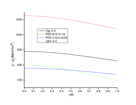
Figure 6: Behaviour of energy conditions vs. fractional radius $r/R$ for case I(first four graph), case II(middle four graph) and case III(last four graph).For plotting this figure we have employed data set values of physical parameters and constants which are the same as used in Fig.1.

Table 1: Numerical values of $R$, M($M_{\odot}$), $C,\,K,$ $\alpha$ and mass-radius ratio of compact star candidates.

Compact star	$R$($km$)	M($M_{\Theta})$	$K$	$C$($km^{-2}$)	$\alpha$	M/R
4U 1820-30	9.316	1.58	-0.4995	0.0023	0	0.25016
Vela X-1	9.561	1.77	-1.097	0.0044	0	0.27306
PSR J1614-2230	9.691	1.97	-0.901	0.0042	0	0.29979
PSR B1913+16	6.6	1.44	-0.798	0.0092	0	0.3218
Cgy X-2	8.31	1.73	-0.8196	0.0055	-0.64	0.30718
PSR B1913+16	6.6	1.44	-0.82	0.0094	-0.81	0.3218
PSR J1614-2230	9.691	1.97	-0.8202	0.0039	-0.36	0.29979
LMC X-4	8.301	1.04	-2.977	0.0055	-2.25	0.1847
Her X-1	8.1	0.85	-1.9779	0.0039	0.0081	0.15475
4U 1538-52	7.866	0.87	-1.9779	0.0045	0.0064	0.16315
SMC X-1	8.831	1.29	-1.9776	0.0052	0.049	0.21547
PSR J1903+327	9.436	1.667	-0.6	0.0027	0.16	0.26057

Table 2: Energy densities and central pressure for different compact star candidates for the above parameter values of Table 1.

Compact star	Central density	Surface density	Central pressure
	$(gm/cm^{3})$	$(gm/cm^{3})$	$(dyne/cm^{2})$	Cases
4U 1820-30	$1.1111\times 10^{15}$	$8.2301\times 10^{14}$	$2.1599\times 10^{35}$	Case I
Vela X-1	$1.3433\times 10^{15}$	$7.7679\times 10^{14}$	$2.9132\times 10^{35}$	Case I
PSR J1614-2230	$1.4324\times 10^{15}$	$8.3109\times 10^{14}$	$2.3899\times 10^{35}$	Case I
PSR B1913+16	$3.3229\times 10^{15}$	$1.9214\times 10^{15}$	$6.3267\times 10^{35}$	Case I
Cgy X-2	$1.9754\times 10^{15}$	$1.1652\times 10^{15}$	$5.2986\times 10^{35}$	Case II
PSR B1913+16	$3.3421\times 10^{15}$	$1.9142\times 10^{15}$	$9.9917\times 10^{35}$	Case II
PSR J1614-2230	$1.4049\times 10^{15}$	$8.4066\times 10^{15}$	$3.7181\times 10^{35}$	Case II
LMC X-4	$1.1903\times 10^{15}$	$7.0236\times 10^{15}$	$1.057\times 10^{35}$	Case II
Her X-1	$0.9538\times 10^{15}$	$6.5385\times 10^{14}$	$0.8032\times 10^{35}$	Case III
4U 1538-52	$1.0957\times 10^{15}$	$7.2461\times 10^{14}$	$0.9751\times 10^{35}$	Case III
SMC X-1	$1.2434\times 10^{15}$	$7.1815\times 10^{14}$	$1.6685\times 10^{15}$	Case III
PSR J1903+327	$1.1683\times 10^{15}$	$8.1755\times 10^{14}$	$2.5073\times 10^{15}$	Case III

9 Adiabatic index

The stability of the relativistic as well as non relativistic compact object likewise relies on the adiabatic index $\gamma$. Heintzmann and Hillebrandt [14] recommended that the adiabatic index must be more than $\frac{4}{3}$ at all interior point of relativistic compact object. In other side the non-relativistic and isotropic case (Newtonian fluids), neutron spherical object system has no upper mass limit for the adiabatic index $\gamma>\frac{4}{3}$ [68]. So, the relativistic radial adiabatic index is defined by[69]

$$\gamma_{r}=\Big{(}\dfrac{\rho+p_{r}}{p_{r}}\Big{)}\dfrac{dp_{r}}{d\rho}$$

Chan et al.[69] obtained the collapsing condition for the ratio of specific heat for an anisotropic fluid distribution as

$$\gamma\leq\frac{4}{3}\Bigg{[}1-max\Bigg{(}\dfrac{p_{r}-p_{t}}{r\mid p_{r}\mid}\Bigg{)}\Bigg{]}$$

From above expression, we can say that the unstable profile of $\gamma$ depend on the anisotropic factor i.e, $\gamma$ will increase when $\Delta>0$ and decrease when $\Delta<0$. Also it is possible that sign of $\Delta$ may be change within the configuration. If it is happen then there is existence of both stable and unstable profile of the object which could lead to fragmentation of the sphere[69]. We can see from Fig.7 that the value of radial adiabatic index is more than $\frac{4}{3}$ at all interior points for each different compact star model.

Figure 7: Behaviour of redshift and adiabatic index vs. fractional radius $r/R$ for case I(first column), case II(second column) and case III(third column).For plotting this figure we have employed data set values of physical parameters and constants which are the same as used in Fig.1.

10 Harrison–Zeldovich–Novikov stability criterion

For any solution representing stable compact stars, like PSR J1614-2230, Her X-1, Cgy X-2 etc., have to fulfill the stability criterion[70, 71]. In this criterion, it is postulate that the any stellar configuration has an increasing mass with increasing central density, i.e. $dM/d\rho_{c}>0$ represents stable configuration and vice versa. If the mass remains constant with increasing central density, i.e. $dM/d\rho_{c}=0$ we get the turning point between stable and unstable region. For this model, we obtained $M(R)$ and $dM/d\rho_{c}$ as follows-

Figure 8: Behaviour of Mass vs. central density and $dM/d\rho_{c}$ vs. central density for case I(first column), case II(second column) and case III(third column). For plotting this figure we have employed data set values of physical parameters and constants which are the same as used in Fig.1.

$$M(R)=\frac{4\,\pi\,\rho_{c}\,R^{3}\,(K-1)}{(3(K-1)+8\,\pi\,K\,\rho_{c}\,R^{2})}~{}~{}~{}~{}~{}\textrm{and}~{}~{}~{}~{}\frac{dM}{d\rho_{c}}=\frac{12\,\pi\,R^{3}\,(K-1)^{2}}{(3(K-1)+8\,\pi\,K\,\rho_{c}\,R^{2})^{2}}$$ (43)

Hence from Fig.8, we can conclude that presenting model represents static stable configuration.

11 Conclusion

In this article, we obtained a new class of well behaved anisotropic compact star models after prescribing Buchdahl metric potential and anisotropic factor. In the present stellar model, we demonstrate that the energy density $\rho$, the radial pressure $p_{r}$ and the tangential pressure $p_{t}$ are completely finite and positive quantities within the stellar configuration, which is shown in Fig.1. So from this figure, we can say that our stellar system is completely free of any physical and geometric singularities. The anisotropy of the stellar model is represented in Fig.2, which exhibit, that anisotropy increases as the radius increases. For instance, the anisotropy is minimum, i.e., zero at the origin and maximum on the surface of the stellar system. The ratios of pressure and density $\dfrac{p_{r}}{\rho},$ $\dfrac{p_{t}}{\rho},$ are monotonically decreasing towards the surface which is outlined in Fig. 2. The model is satisfy the following dominant energy conditions(see Fig.6) (i) strong energy condition(SEC) (ii) weak energy condition(WEC) and (iii) null energy condition(NEC). In current study the redshift is also decreasing from the center to surface (see Fig.7). From the point of view of causality condition the stellar model is completely stable, because the square of sound speed is less than 1 everywhere within the star (Fig.3), besides there is no change in sign $v^{2}_{r}-v^{2}_{t}$ and stability factor ($v^{2}_{t}-v^{2}_{r}$) lies between -1 and 0 for stable configuration and 0 to 1 for unstable configuration (Fig.3).The static stable criterion also hold good by our solutions(see Fig.8) Moreover, the relativistic adiabatic index $\gamma_{r}$ is greater than $\frac{4}{3}$ and monotonically increasing towards the surface. On the other hand, the compact stellar model is in equilibrium under three different forces, namely the gravitational force $F_{g}$, the hydrostatic force $F_{h}$, and the anisotropic force $F_{a}$ (Fig.5). The latest one causes a repulsive force that counteracts the gravitational gradient, this is so because we are in the presence of a positive anisotropy factor $\Delta_{1}\,,\Delta_{2}\,,\Delta_{3}$ as can be seen in Fig 2. Based on physical requirements, we match the interior solution to an exterior vacuum Schwarzschild spacetime on the boundary surface at $r=R,$ and from the comparison of both side metrics, all constants are determined which are listed in Table 1. By using these constants in our investigation for several analogue objects with similar mass and radii, namely, PSR J1614-2230, PSR B1913+16, Cgy X-1, LMC X-4, Vela X-1, 4U 1820-30, 4U 1538-52, SMC X-1, PSR J1903+327 and Her X-1. Whereas, Table 2 contains the central pressure, central and surface energy density is within the parameter outlined in Table 1.

References

- [1] K. Schwarzschild, Sitz. Deut. Akad. Wiss. Berlin, Kl. Math. Phys. 24, 424 (1916)
- [2] R.C. Tolman, Phys. Rev. 55, 364 (1939)
- [3] J.R. Oppenheimer, G.M. Volkoff, Phys. Rev.55, 374 (1939)
- [4] B.V Ivanov, Phys.Rev.D 65 104001 (2002)
- [5] Y.K. Gupta, N. Kumar, Gen. Relativ. Gravit. 37(1),575 (2005)
- [6] V. Canuto, Annu. Rev. Astron. Astrophys. 12, 167 (1974)
- [7] V. Canuto, Annu. Rev. Astron. Astrophys. 13, 335 (1975)
- [8] V. Canuto, Ann. N. Y. Acad. Sci. U.S.A. 302, 514 (1977)
- [9] V. Canuto, M. Chitre, Phys. Rev. Lett. 30, 999 (1973)
- [10] V. Canuto, S.M. Chitre, Phys. Rev. D 9, 1587 (1974)
- [11] V. Canuto, J. Lodenquai, Phys. Rev. D 11, 233 (1975)
- [12] R. Ruderman, Ann. Rev. Astron. Astrophys. 10,427 (1972)
- [13] R.L. Bowers,E.P.T. Liang, Astrophys. J. 188, 657 (1974)
- [14] H. Heintzmann, W. Hillebrandt, Astron. Astrophys.38, 51 (1975)
- [15] M. Cosenza, L. Herrera, M. Esculpi, L. Witten, J. Math. Phys. 22, 118 (1981)
- [16] M. Cosenza, L. Herrera, M. Esculpi, L. Witten, Phys. Rev. D 25, 2527 (1982)
- [17] M. K. Mak, T. Harko, Proc. Roy. Soc. Lond. A 459, 393 (2003)
- [18] R. K. Kippenhahm, A. Weigert, Stellar Structure and Evolution (Springer, Berlin, 1990), p. 384.
- [19] R. F. Sawyer, Phys. Rev. Lett. 29, 382 (1972)
- [20] A. I. Sokolov, JETP 79, 1137 (1980)
- [21] R. Sharma and S. D. Maharaj, Mon. Not. R. Astron. Soc.375, 1265 (2007)
- [22] L. Herrera, W. Barreto, Phys. Rev. D 88, 084022 (2013)
- [23] D. Deb, S. R. Chowdhury, S. Ray, F. Rahaman, B. K. Guha, Ann. Phys. (Amsterdam) 387, 239 (2017)
- [24] V. Varela, F. Rahaman, S. Ray, K. Chakraborty, M. Kalam, Phys. Rev. D 82, 044052 (2010)
- [25] B. V. Ivanov, Eur. Phys. J. C 78, 332 (2018)
- [26] A. Nasim, M. Azam, Eur. Phys. J. C 78, 34 (2018)
- [27] A. A. Isayev, Phys. Rev. D 96, 083007 (2017)
- [28] B. V. Ivanov, Eur. Phys. J. C 77, 738 (2017)
- [29] P. C. Vaidya, R. Tikekar, J. Astrophys. Astron. 3, 325 (1982)
- [30] R. Tikekar, J. Math. Phys. (N.Y.) 31, 2454 (1990)
- [31] K. Komathiraj, S. D. Maharaj, J. Math. Phys. (N.Y.) 48, 042501 (2007)
- [32] L. K. Patel, S. S. Kopper, Aust. J. Phys. 40, 441 (1987)
- [33] R. Sharma, S. Mukherjee, S. D. Maharaj, Gen. Relativ. Gravit. 33, 999 (2001)
- [34] R. Finch, J. E. F. Skea, Classical Quantum Gravity 6, 467 (1989)
- [35] M. S. R. Delgaty, K. Lake, Comput. Phys. Commun.115, 395 (1998)
- [36] L. Herrera, A. Di Prisco, J. Ospino, E. Fuenmayor, J. Math. Phys. (N.Y.) 42, 2129 (2001)
- [37] B. C. Paul,S. Dey, Astrophys. Space Sci. 363, 220 (2018)
- [38] B. C. Paul, P. K. Chattopadhyay, and S. Karmakar, Astrophys. Space Sci. 356, 327 (2015)
- [39] S. D. Maharaj, D. K. Matondo, P. M. Takisa, Int. J. Mod. Phys. D 26, 1750014 (2017)
- [40] P. Demorest, T. Pennucci, S. M. Ransom, M. S. E. Roberts, J.W. T. Hessels, Nature (London) 467, 1081 (2010)
- [41] M. L. Rawls, J. A. Orosz, J. E. McClintock, M. A. P. Torres, C. D. Bailyn, M. M. Buxton, Astrophys. J. 730, 25 (2011)
- [42] R. L. Kelley, J. G. Jernigan, A. Levine, L. D. Petro, S. Rappaport, Astrophys. J. 264, 568 (1983)
- [43] M. K. Abubekerov, E. A. Antokhina, A.M. Cherepashchuk, V. V. Shimanskii, Astronomy Reports 52 , 379 (2008)
- [44] P. C. C. Freire et al., Mon. Not. R. Astron. Soc. 412, 2763 (2011)
- [45] J.M. Weisberg, D.J. Nice, J.H. Taylor, ApJ 722(2),1030 (2010)
- [46] T. Guver, et al., ApJ 712, 964(2010)
- [47] J. Casares, et al., ApJ 493, L39-L42(1998)
- [48] L.D. Landau, E.M. Lifshitz, The classical Theory of Fields, Pergamon Press, Oxford ,England. 225 (1975)
- [49] L. Herrera and J. P. de Leon, J. Math. Phys. (N.Y.) 26, 2302 (1985)
- [50] H.A. Buchdahl, Phys. Rev. D 116, 1027 (1959)
- [51] N. Bijalwan, Y.K. Gupta, Astrophys. Space Sci.334, 293-299 (2011)
- [52] F. Rahaman, S. Ray, A. K. Jafry, and K. Chakraborty, Phys.Rev. D 82, 104055 (2010)
- [53] W.Israel, Nuovo Cimento B 44, 1 (1966);48,463(E)(1967)
- [54] H. Bondi, Proc. R. Soc. A 282, 303 (1964)
- [55] C. G. Bohmer, T. Harko, Gen. Relativ. Gravit. 39, 757 (2007)
- [56] H. Andreasson, Commum. Math. Phys. 198, 507 (2009)
- [57] C. G. Bohmer, T. Harko, Phys. Lett. B 630, 73 (2005)
- [58] J.L. Rosa, P. Picarra, Phys. Rev.D 102, 064009 (2020)
- [59] G. A. Carvalho, R. M. Marinho Jr., M. Malheiro, J. Phys. Conf. Ser. 630 , 012058 (2015)
- [60] J. Lattimer, Annu. Rev. Nucl. Part. Sci. 62, 485 (2012)
- [61] T. Gangopadhyay, et al., Monthly Notices of the Royal Astronomical Society, 431, 3216-3221 (2013)
- [62] S. Karmakar, S. Mukherjee, R. Sharma, S. D. Maharaj, Pramana 68, 881 (2007)
- [63] D. E. Barraco, V. H. Hamity, R. J. Gleiser, Phys. Rev. D 67, 064003 (2003)
- [64] L. Herrera, Phys. Lett. A 165, 206 (1992)
- [65] H. Abreu, H. Hernandez, L.A. Nunez, Class. Quantum Grav. 24, 4631 (2007)
- [66] J. Ponce de Leòn, Gen. Relat. Gravit. 25, 1123 (1993)
- [67] M. Visser, Lorentzian Wormholes (Springer, Berlin, 1996), p. 115.
- [68] H. Bondi, Mon. Not. R. Astron. Soc. 281, 39 (1964)
- [69] R. Chan, L. Herrera, and N. O. Santos,Mon. Not. R. Astron. 756 Soc. 265, 533 (1993)
- [70] B.K. Harrison,et al.:Gravitational Theory and Gravitational collapse(Chicago:University of Chicago Press-1965)
- [71] Y.B. Zeldovich, I.D. Novikov.: Relativistic Astrophysics Vol 1 : Stars and Relativity(Chicago:University of Chicago Press-1971)