Statistical Mechanics of Systems with Negative Temperature

Abstract

Do negative absolute temperatures matter physics and specifically Statistical Physics? We provide evidence that we can certainly answer positively to this vexata quaestio. The great majority of models investigated by statistical mechanics over almost one century and a half exhibit positive absolute temperature, because their entropy is a nondecreasing function of energy. Since more than half a century ago it has been realized that this may not be the case for some physical systems as incompressible fluids, nuclear magnetic chains, lasers, cold atoms and optical waveguides. We review these examples and discuss their peculiar thermodynamic properties, which have been associated to the presence of thermodynamic regimes, characterized by negative absolute temperatures. As reported in this review, the ambiguity inherent the definition of entropy has recurrently raised a harsh debate about the possibility of considering negative temperature states as genuine thermodynamic equilibrium ones. Here we show that negative absolute temperatures are consistent with equilibrium as well as with non-equilibrium thermodynamics. In particular, thermometry, thermodynamics of cyclic transformations, ensemble equivalence, fluctuation-dissipation relations, response theory and even transport processes can be reformulated to include them, thus dissipating any prejudice about their exceptionality, typically presumed as a manifestation of transient metastable effects.

I Introduction

I.1 Introductory remarks and plan of the paper

Among all physical quantities in thermodynamics and statistical mechanics, temperature has for sure a privileged role. It is the first observable which is introduced in any course on thermodynamics, and it rules the macroscopic behaviour of systems in and out of equilibrium; one of the main aims of statistical mechanics is precisely to establish exact relations between the temperature of a system and its underlying microscopic dynamics. Despite its importance, at a first glance the notion of temperature may appear to be relatively simple, expecially to beginners: the mantra temperature is a quantity proportional to the mean kinetic energy of a particle is often believed to be exhaustive about the whole subject. However, although the statement is correct for most physical systems, one should always keep in mind that the concept of temperature is much more sophisticated than that puglisi17 .

The richness of the notion of temperature and its relation with many important aspects of the statistical description of macroscopic objects are often underestimated. For instance, even in good books of philosophy of science, one can find the naive idea that the relation between temperature and average kinetic energy is the bridge law between mechanics and thermodynamics nagel79 . This is wrong: the expression of temperature in terms of mean kinetic energy holds only for a special class of phenomena, although very important. A more general bridge law is represented by the celebrated relation, engraved on the Boltzmann’s tombstone, between the entropy $S$ and the number of states $W$ which are accessible to the considered system: $S=k_{B}\log W$, where $k_{B}$ is the Boltzmann constant.

An accurate analysis of the concept of temperature, and in particular of its relationship with energy an entropy, shows the possibility, for suitable systems, to attain equilibrium states at negative absolute temperature (NAT). The existence of this class of models is not a mere theoretical curiosity; on the contrary, many important systems, from several branches of physics, belong to this category: vortices in two-dimensional hydrodynamics, magnetic spins and cold atoms in optical lattices are just some examples. For such systems, NAT states have been observed in real laboratory experiments.

In the last decades, much work was devoted to the theoretical understanding of such unusual thermal states. Starting from the pioneering works by Onsager onsager49 and Ramsey ramsey56 , who originally introduced the physical idea and the first theoretical analyses, many authors have discussed the consequences of including negative temperature in the building of thermodynamics and statistical mechanics. Equilibrium and out-of-equilibrium situations have been analysed and compared to the familiar cases with positive temperature, leading to a large body of work on the subject. Some authors have also criticised the concept of negative temperature, for several reasons, raising an interesting debate on the very foundations of statistical mechanics.

In this review we aim at providing a picture of the state of the art on this wide subject, trying to clarify the fundamental theoretical aspects and the open controversies, discussing results from classical works on the subject as well as the most recent findings. In the remaining part of this Section we give a brief overview on the concept of temperature, for a generic Hamiltonian system, focusing on the relation between energy and entropy and the conditions to observe negative absolute temperatures. In Section II we give an account of the most important examples of physical systems which can be found in NAT states; some relevant experimental aspects are briefly mentioned and discussed. Section III reports the main points of the interesting debate on the consistency of negative tempertaure: alternative proposals for the statistical interpretation of entropy and temperature, which would rule out the possibility of NAT equilibrium states, are analysed in some detail; the problem of thermodynamic cycles at negative tempertaure is also discussed. In Section IV we describe the main aspects of equilibrium states at negative temperature, and we introduce in this context some mechanical models which are paradygmatic for this class of systems; particular attention is given to the problem of measuring temperature and to the equivalence between statistical ensembles (and its violations). Section V is devoted to the analysis of the fluctuation-dissipation relation when NAT states are allowed; Langevin equation and response theory are revised, and the possibility to design thermal baths at negative temperature is discussed. Section VI accounts for the large body of works on the Discrete Non-Linear Schrödinger Equation, an important physical model which shows a rich and nontrivial phenomenology, which also includes states at NAT. Finally in Section VII we discuss some recent results and open questions on the problem of heat transport in one-dimensional systems, when also negative temperatures are present.

I.2 Entropy and temperature

When pondering about the foundations of thermodynamics and statistical mechanics, one is often left with the feeling that the very constitutional concepts of those theories, as entropy and temperature, are not easy at all to master, even in equilibrium conditions. As clearly expressed by Truesdell truesdell13 :

Entropy, like force, is an undefined object, and if you try to define it, you will suffer the same fate as the force definers of the seventeenth and eighteenth centuries. Either you will get something too special or you will run around in a circle.

One may be tempted to say that, since thermodynamics is a phenomenological theory, it is somehow unavoidable that also its primitive concepts only refer to practical experience; in this light, it seems natural to introduce all fundamental quantities via proper operative definitions, so that, for instance, temperature should be only seen as the result of a measuring protocol involving some kind of thermometer. While this point of view is, without any doubt, largely satisfactory at a pragmatic level (e.g. in most engineering applications), from a more conceptual perspective it can actually raise some concern.

Indeed, we know that macroscopic systems are made of particles (atoms, molecules) ruled by microscopic mechanical laws. In the eighteenth century, physicists started to understand the necessity of a clear link between the mechanical world (i.e. Newtons’s laws, in the classical description) on the one hand, and the phenomena described by thermodynamics on the other. As far as we know, the first attempt in this direction is due to Daniel Bernoulli. In his seminal book Hydrodynamica, he considered ideal gases constituted by point-like particles of mass $m$: the pressure resulted then as a consequence of the many collisions of the molecules with the walls of the container hall03 . Using this model for gaseous matter, Clausius was able to show that temperature $T$ is proportional to the mean kinetic energy of the system:

$$m\langle v^{2}\rangle=k_{B}T$$ (1)

being $v$ any component of the velocity, and $k_{B}$ the Boltzmann constant (in modern terminology).

The decisive step to understand the relation between mechanics and thermodynamics was made by Ludwig Boltzmann by introducing ergodicity, i.e. by assuming that an isolated mechanical systems will eventually explore, in a homogeneous way, the whole fixed-energy hypersurface accessible to it in the space of its configurations. This assumption, which turns out to be true for almost all practical purposes, allowed him to make a precise connection between the microscopic world and the macroscopic, observable quantities of thermodynamics; this relation is summarized by the celebrated equation:

$$S(E)=k_{B}\log W(E)\,,$$ (2)

engraved on Boltzmann’s tombstone. Here $S(E)$ denotes the entropy of the macroscopic body and $W(E)$ is the number of microscopic states accessible to the system, once a proper discretization of the phase-space has been introduced. Since $S$ is a thermodynamic observable, while $W$ is clearly a mechanical-like quantity, in the terminology of the philosophy of science Eq. (2) is a bridge law between mechanics and thermodynamics.

Given a system with Hamiltonian $\mathcal{H}(\mathbf{Q},\mathbf{P})$, to understand its macroscopic behaviour we must first express $W(E)$ as a function of the energy $E$ and of the other parameters of the system, and then compute the entropy through Eq. (2). $W(E)$ is obviously proportional to the density of states

$$\omega(E)=\int\mathcal{D}\mathbf{Q}\mathcal{D}\mathbf{P}\,\delta(E-\mathcal{H}(\mathbf{Q},\mathbf{P}))\,,$$ (3)

so that Eq. (2) is usually written as

$$S(E)=k_{B}\log\omega(E)\,.$$ (4)

Even if this designation is not historically precise mehra01 , the above quantity is sometimes referred to as “Boltzmann entropy”. In the following we shall adopt this convention. Once entropy is known, the thermodynamic relations can be invoked to find all interesting thermodynamic quantities. In particular, the well known relation

$${1\over T}={\partial S\over\partial E}$$ (5)

can be used to obtain a mechanical definition of temperature which is usually found in Statistical mechanics textbooks ma85 ; huang88 and which we shall refer to as “Boltzmann temperature”.

The deep connection between Boltzmann entropy (and temperature) and the corresponding thermodynamic counterpart can be understood by recalling the following, straightforward argument. Let us consider two independent systems $\mathcal{A}$ and $\mathcal{B}$, at energy $E_{\mathcal{A}}$ and $E_{\mathcal{B}}$ respectively. It is a trivial consequence of Eq. (2) that the compound system $\mathcal{A}\cup\mathcal{B}$ has a total entropy

$$S_{A\cup B}=S_{\mathcal{A}}(E_{\mathcal{A}})+S_{\mathcal{B}}(E_{\mathcal{B}})\,.$$ (6)

Let us now assume that the two subsystems $\mathcal{A}$ and $\mathcal{B}$ are now put into thermal contact, i.e. they are allowed to exchange energy with each other, still being isolated from the environment. We also assume that contributions to the total energy $E=E_{\mathcal{A}}+E_{\mathcal{B}}$ coming from the interaction among the two systems can be neglected, a condition typically verified when only short-range interactions are involved. The equilibrium condition is reached when $S_{\cup}$ is maximized with respect to $E_{\mathcal{A}}$ (and $E_{\mathcal{B}}=E-E_{\mathcal{A}}$), i.e when

$$\frac{\partial S_{\mathcal{A}}}{\partial E_{\mathcal{A}}}=\frac{\partial S_{\mathcal{B}}}{\partial E_{\mathcal{B}}}\,.$$ (7)

It is therefore clear that $\partial S/\partial E$ has a straightforward interpretation as (an invertible function of) the temperature of a system at equilibrium, if $S$ is the Boltzmann entropy.

Let us anticipate that in Section III.1 we shall examine a possible alternative definition of entropy, and temperature, attributed to Josiah Willard Gibbs. Even though, as we will discuss in the following, this alternative description has several interesting properties, it fails, in our opinion, to give an interpretation of equilibrium temperature as straightforward as that exposed above: this is the main reason why, in this review, we shall mainly refer to the standard Boltzmann formalism. We need to specify this point because, for the physical systems discussed in the following, the two “entropies” (and the two “temperatures”) show completely different behaviors, even in the thermodynamic limit: in particular, as we will discuss, the Gibbs temperature is always positive, by definition; the Boltzmann temperature, on the other hand, can assume negative values in the high-energy regime, for some classes of physical systems. These “negative-temperature” states are the main subject of the present review.

I.3 Negative absolute temperature

From the discussion of the above section it is clear that the Boltzmann temperature assumes negative values whenever the density of states $\omega(E)$, defined by Eq. (3), shows a negative slope. If this is the case, in that interval also entropy is a decreasing function of energy, and Eq. (5) assures that the absolute temperature is negative. This possibility may sound quite unusual or even paradoxical, for sure very far from everyday experience. In Section II we shall illustrate some relevant examples of physical systems in which thermodynamic states at NAT appear; for now, let us just discuss why they are not as common as positive-temperature states.

Consider an isolated system described by the generic Hamiltonian

$$\mathcal{H}(\mathbf{Q},\mathbf{P})=\sum_{i=1}^{N}\frac{p_{i}^{2}}{2m}+\mathcal{U}(\mathbf{Q})\,,$$ (8)

where $\mathcal{U}$ is the potential contribution to the Hamiltonian, a regular function of (in general) all positions and bounded from below (stability condition); without any lack of generality, we can assume that $\min_{\mathbf{Q}}\mathcal{U}(\mathbf{Q})=0$. We also assume that the only quantity conserved by dynamics is the total energy $E$. The density of states of this system can be written as

$$\begin{split}\omega(E)&=\int\mathcal{D}\mathbf{Q}\mathcal{D}\mathbf{P}\,\delta(E-\mathcal{H}(\mathbf{Q},\mathbf{P}))\\ &=\int\mathcal{D}\mathbf{Q}\mathcal{D}\mathbf{P}\,\int_{0}^{E}du\,\delta(u-\mathcal{U}(\mathbf{Q}))\delta\left(E-u-\sum_{i=1}^{N}\frac{p_{i}^{2}}{2m}\right)\,.\end{split}$$ (9)

Due to the quadratic form of the kinetic energy, we can explicitly compute the integral over the momenta; as a result, we obtain

$$\omega(E)=\int_{0}^{E}du\,\omega_{\mathbf{Q}}(u)c_{N}(E-u)^{N/2-1}\,,$$ (10)

where $c_{N}=\frac{N}{2}(2\pi)^{N/2}/\Gamma(1+N/2)$ is a constant (being $\Gamma(x)$ the Euler Gamma function). In the above equation we have introduced a “configurational” $\omega_{\mathbf{Q}}$ density of states only depending on positions, i.e.

$$\omega_{\mathbf{Q}}(u)=\int\mathcal{D}\mathbf{Q}\,\delta(u-\mathcal{U}(\mathbf{Q}))\,.$$ (11)

By deriving Eq. (10) with respect to the energy, we obtain, for $N>4$,

$$\omega^{\prime}(E)=\frac{(N-2)c_{N}}{2}\int_{0}^{E}du\,\omega_{\mathbf{Q}}(u)(E-u)^{N/2-2}\geq 0\,,$$ (12)

the last inequality coming from the positivity of $\omega_{\mathbf{Q}}(u)$.

The above argument should clarify why in most physical systems only positive-temperature states can be observed: as far as the dynamics of the system can be modeled by a Hamiltonian with quadratic kinetic terms, with potential energy not depending on momenta and no additional conserved quantities, the density of states is always an increasing function of the energy. As a consequence, entropy is also monotonic and temperature can never assume negative sign.

Negative temperatures are instead typically observed in systems with bounded phase spaces, some of which will be discussed in the next Section. In most cases, two regimes can be identified: at low energy, $\omega(E)$ is usually an increasing function, since additional energy allows the system to explore wider regions of the phase space; but since the phase-space volume is finite, the number of states cannot increase indefinitely, and it must exist some energy threshold $E^{*}$ such that, for $E>E^{*}$, $\omega(E)$ starts decreasing. Introducing the inverse temperature

$$\beta=\frac{1}{k_{B}}\frac{\partial S}{\partial E}$$ (13)

we can summarize this typical scenario as follows:

$$\begin{cases}E<E^{*}\,,\quad\beta>0\quad\longrightarrow\quad T>0\\ E=E^{*}\,,\quad\beta=0\quad\longrightarrow\quad T\to\pm\infty\\ E<E^{*}\,,\quad\beta<0\quad\longrightarrow\quad T<0\,.\end{cases}$$ (14)

The situation is qualitatively sketched in Fig. 1, where the typical entropy vs energy curve of usual systems with quadratic kinetic energy is compared to that of systems with bounded phase space. As we are going to show in what follows, this qualitative scenario concerns also models other than those with bounded phase space, like the Discrete Nonlinear Schrödinger Equation (See Sections II.5 and III.3.5).

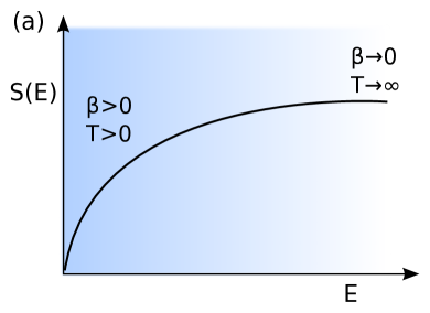
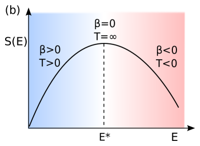
Figure 1: Qualitative sketch of the entropy vs energy curve for systems with unbounded phase space (panel (a)) and for typical cases with bounded phase space (panel (b)).

Some confusion may arise from the fact that, according to the above discussion, any system with $T<0$ is, to the purpose of establishing the energy flux, “hotter” than any other system with $T>0$. To clarify this point, let us consider again two systems ${\cal A}$ and ${\cal B}$, composed by $N_{{\cal A}}$ and $N_{{\cal B}}$ particles and described by the Hamiltonians $\mathcal{H}_{{\cal A}}({\bf Q}_{{\cal A}},{\bf P}_{{\cal A}})$ and $\mathcal{H}_{{\cal B}}({\bf Q}_{{\cal B}},{\bf P}_{{\cal B}})$, respectively. Here we limit ourselves to the case in which $\mathcal{H}_{{\cal A}}$ and $\mathcal{H}_{{\cal B}}$ have the same functional dependencies on the canonical variables (i.e. they correspond to systems with the same microscopic dynamics, with possibly different sizes $N_{{\cal A}}$ and $N_{{\cal B}}$), and only short-range interactions are involved. Using the additivity of entropy, in the thermodynamic limit we can introduce the entropy per particle $s(e)$

$$s(e)=\frac{S(E,N)}{N}\,,$$ (15)

where $e$ is the specific energy. With our assumptions, $s(e)$ has the same functional form in the two systems.

Let us now suppose that systems ${\cal A}$ and ${\cal B}$ have energy $E_{{\cal A}}=N_{{\cal A}}e_{{\cal A}}$ and $E_{{\cal B}}=N_{{\cal B}}e_{{\cal B}}$ respectively, and that the corresponding inverse temperatures are $\beta_{\cal A}$ and $\beta_{\cal B}$. When the two systems are put in contact via some kind of small, short-range interaction, a new system is realized, composed by $N=N_{{\cal A}}+N_{{\cal B}}$ particles. If we denote by $a=N_{{\cal A}}/N$ the fraction of particles from the system ${\cal A}$, the final energy that the total system achieves at equilibrium is clearly

$$E_{f}=Ne_{f}\,,\quad\text{with}\quad e_{f}=ae_{{\cal A}}+(1-a)e_{{\cal B}}\,.$$ (16)

Since, according to ergodic hypothesis, the system will spend most time in the macroscopic state which corresponds to the largest number of microscopic configurations, the final entropy reached by the system cannot be smaller than the initial one:

$$Ns(e_{f})\geq N_{{\cal A}}s(e_{{\cal A}})+N_{{\cal B}}s(e_{{\cal B}})=N[as(e_{{\cal A}})+(1-a)s(e_{{\cal B}})]\,;$$ (17)

this is consistent with the second principle of thermodynamics. Note that the specific entropy of the global system is the same as those of the subsystems, due to our assumption that the interacting potentials are short-range. The previous inequality is nothing but a way to express the concavity of $s(e)$:

$$s(ae_{{\cal A}}+(1-a)e_{{\cal B}})\geq as(e_{{\cal A}})+(1-a)s(e_{{\cal B}})\,.$$ (18)

As a consequence, the inverse temperature $\beta$ is a monotonically decreasing function of the energy. The final inverse temperature $\beta_{f}$ is intermediate between $\beta_{\cal A}$ and $\beta_{\cal B}$, i.e. if $e_{{\cal B}}>e_{{\cal A}}$, that is $\beta_{\cal A}>\beta_{\cal B}$, then

$$\beta_{\cal B}<\beta_{f}<\beta_{\cal A}\,\,.$$ (19)

The energy flux obviously goes from smaller to larger $\beta$, i.e. from hot to cold, irrespectively of the sign of $\beta$. The absolute temperature $T=(k_{B}\beta)^{-1}$ fails to verify an analogous ordering; and indeed the privileged role of $\beta$ over $T$ in statistical mechanics is also quite clear if one notes that $\beta$ is the variable actually associated to energy, e.g. when passing from microcanonical to canonical ensemble. The fact that we use $T$, instead of $\beta$, as a measure of thermal equilibrium may be seen as an historical heritage of the first phenomenological studies on thermodynamics, but it has no fundamental reason.

Let us now conclude this section by briefly discussing the case in which two different systems $\mathcal{A}$ and $\mathcal{B}$ are put at contact, assuming that $\mathcal{A}$ can admit negative temperature, while $\mathcal{B}$ cannot. It is quite easy to understand that the coupling of the system $\mathcal{A}$, initially prepared in a negative temperature state, with the system $\mathcal{B}$, always at positive temperature, will result in a system with final positive temperature. Indeed, by repeating the argument discussed in the previous section, we find that at equilibrium the relation

$$\beta_{\mathcal{A}}={\partial S_{\mathcal{A}}\over\partial E_{\mathcal{A}}}={\partial S_{\mathcal{B}}\over\partial E_{\mathcal{B}}}=\beta_{\mathcal{B}}$$ (20)

must hold. Since $\beta_{\mathcal{B}}$ is positive for every value of $E_{\mathcal{B}}$, the final common temperature must also be positive. The above result helps to understand why it is not common to observe negative temperature: even if one deals with systems allowed to achieve such kind of states, it is necessary to completely isolate them from the external environment, made by ordinary matter which can only assume positive temperature. In Section IV.2 we shall consider again this aspect from a theoretical point of view. This difficulty is crucial in experimental contexts, where one has the practical need to isolate the system from the environment, at least for a time long enough to allow for internal equilibration, as we will briefly see in the next section.

II Examples and phenomenology

II.1 Onsager’s vortices

One of the first, and most important, systems showing negative temperature was studied by Onsager in a seminal paper at the origin of the modern statistical hydrodynamics onsager49 . Due to the historical and technical relevance of that work, it is worth to briefly summarize its main results.

Consider a two-dimensional incompressible ideal flow in a domain $\mathcal{A}$. The time evolution of the flow ${\bf u}$ is ruled by Euler equation

$$\begin{cases}\partial_{t}{\bf u}+({\bf u}\cdot\nabla){\bf u}=-\frac{\nabla p}{\rho_{0}}\\ \nabla\cdot{\bf u}=0\,,\end{cases}$$ (21)

being $\rho_{0}$ and $p$ the constant density and the pressure of the fluid, respectively. Let us introduce the vorticity $w$, defined by

$$\nabla\times{\bf u}=w\hat{\bf z}\,,$$ (22)

where $\hat{\bf z}$ is the unitary vector perpendicular to the plane of the flow. From Eq. (21) one has that $w$ evolves according to

$$\partial_{t}w+({\bf u}\cdot\nabla)w=0\,\,.$$ (23)

The previous equation is nothing but the conservation of vorticity along fluid-element paths kraichnan80 . The incompressibility condition allows us to introduce the stream function $\psi$:

$${\bf u}=\nabla^{\perp}\psi=(\partial_{y},-\partial_{x})\psi\,,\quad\quad w=-\Delta\psi\,.$$ (24)

Therefore, the velocity can be expressed in terms of $w$ as

$${\bf u}({\bf x},t)=-\nabla^{\perp}\int d{\bf x}^{\prime}{\cal G}({\bf x},{\bf x}^{\prime})w({\bf x}^{\prime},t)$$ (25)

where ${\cal G}({\bf r},{\bf r}^{\prime})$ is the Green function of the Laplacian operator $\Delta$, which depends on the shape of the domain $\mathcal{A}$.

Consider now an initial condition at $t=0$ such that the vorticity is localized on $N$ point-vortices

$$w({\bf r},0)=\sum_{i=1}^{N}\Gamma_{i}\delta({\bf r}-{\bf r}_{i}(0))\,\,,$$ (26)

where $\Gamma_{i}$ is the circulation of the $i-$th vortex. Using the Kelvin theorem truesdell18 one realizes that the vorticity must remain localized at any time:

$$w({\bf r},t)=\sum_{i=1}^{N}\Gamma_{i}\delta({\bf r}-{\bf r}_{i}(t))\,.$$ (27)

Plugging the above formula in Eq. (23) it is possible to derive the evolution law for the vortex positions ${\bf r}_{i}=(x_{i},y_{i})$:

$$\frac{dx_{i}}{dt}=\frac{1}{\Gamma_{i}}\frac{\partial\mathcal{H}}{\partial y_{i}}\,\,\,,\,\,\,\frac{dy_{i}}{dt}=-\frac{1}{\Gamma_{i}}\frac{\partial\mathcal{H}}{\partial x_{i}}\,\,\,,$$ (28)

with

$$\mathcal{H}(\mathbf{r}_{1},\dots,\mathbf{r}_{N})=\sum_{i\neq j}\Gamma_{i}\Gamma_{j}{\cal G}({\bf r}_{i},{\bf r}_{j})\,.$$ (29)

So the $N$ point vortices constitute a $N$ degree of freedom Hamiltonian system newton10 with canonical coordinates

$$q_{i}=\sqrt{|\Gamma_{i}|}x_{i}\,,\quad p_{i}=\text{sign}(\Gamma_{i})\sqrt{|\Gamma_{i}|}y_{i}\,\,.$$ (30)

and the corresponding Hamiltonian $\mathcal{H}(\mathbf{Q},\mathbf{P})=H[\mathbf{r}_{1}(q_{1},p_{1}),\dots,\mathbf{r}_{N}(q_{N},p_{N})]$

Consider now $N$ point vortices confined in a bounded domain $\mathcal{A}$ of area $A$. Since for each point vortex ${\bf r}_{i}\in\mathcal{A}$ one has that the phase-space volume enclosed by the constant-energy hypersurface $\mathcal{H}(\mathbf{X},\mathbf{Y})=E$ verifies

$$\Omega(E)=\int_{\mathcal{H}<E}dq_{1}\cdots dq_{N}dp_{1}\cdots dp_{N}\leq C_{N}A^{N}\,,\quad C_{N}=\prod_{i=1}^{N}|\Gamma_{i}|\,,$$ (31)

it follows that the density of states $\omega(E)=d\Omega(E)/dE$ must approach to zero for $E\to\pm\infty$, and it must therefore attain its maximum at a certain finite value $E_{M}$. This implies that for $E>E_{M}$ the entropy $S(E)=k_{B}\ln\omega(E)$ is a decreasing function and hence $T(E)=(dS/dE)^{-1}$ is negative.

It is easy to understand that both the low- and high-energy regimes, corresponding to $\beta\gg 1$ and $\beta\ll-1$, are characterized by spatially ordered configurations. Indeed, in any finite domain $\mathcal{A}$, for ${\bf r}\sim{\bf r}^{\prime}$ we have ${\cal G}({\bf r},{\bf r}^{\prime})\simeq-1/(2\pi)\ln|{\bf r}-{\bf r}^{\prime}|$, and the energy contribution of a pair of vortices located in ${\bf r}$ and ${\bf r}^{\prime}$ is maximized, in modulus, if they are very close to each other. The sign of the energy contribution is, of course, determined by the sign of the vorticities. As a result, when energy is small, $E\ll E_{M}$, the system tends to organize itself into pairs of very close vortices with opposite signs of $w$; at large energy $E\gg E_{M}$, on the other hand, the typical states are those in which the vortices are crowded in two separate clusters, depending on the sign of their vorticity onsager49 ; kraichnan80 ; newton10 . Let us notice that in the negative-temperature scenario energy tends to be transferred from small-scale structures (wandering pairs of opposite-sign vortices) to a large-scale configuration (two clusters containing almost all vortices). This mechanism is somehow opposite to what usually happens in three-dimensional turbulence, where energy is carried from large to small spatial scales: this phenomenon is therefore called “inverse energy cascade”.

The model proposed by Onsager has been studied in many works, both analytically and numerically. It has been shown, for instance, that it is possible to derive a canonical distribution for a small portion of the system even at negative temperature; in the same context, an attempt to solve the BBGKY hierarchy for the distribution of the vorticity was discussed, using the Vlasov approximation montgomery74 . Similar studies were done in the context of guiding-center plasma, that can be modeled with the same equations of point vortices in two-dimensional hydrodynamics smith89 ; smith90 .

In the 70’s, early numerical simulations of Eq. (28) supported the picture that negative temperature would signal the emergence of a new ordered phase at high energies montgomery74 . Nowadays modern computational tools allow for much more extensive simulations of the vortices dynamics, and the underlying physical mechanisms can be efficiently observed and studied yatsuyanagi05 ; yatsuyanagi15 . As predicted by Onsager, in the $\beta<0$ regime, negative and positive vortices separate into two large clusters.

In more recent years, the above theory has been adopted and studied in the context of quantum superfluids simula14 ; groszek17 ; valani18 . In particular it has been shown by numerical simulations that isolated Bose-Einstein condensates, under suitable conditions, relax towards the ordered phase at negative temperature described by Onsager. The mechanism behind the formation of large clusters of equal sign vortices is the so-called “evaporative heating”. From time to time, pairs of opposite-sign vortices happen to melt together and disappear, while their energy is transferred to the other vortices through the produced sound waves. During such process the energy of the system is conserved, but the entropy of the vortices decreases, due to the disappearing of a pair simula14 .

Experimental evidences of inverse energy cascade and of hydrodynamics states at negative temperature have been reported in two very recent works gauthier19 ; johnstone19 . The two research groups have realized, independently of each other and using different methodologies, experimental setups that allow for the observation of vortices in superfluid Bose-Einstein condensates. In both cases, steady large-scale clusters of vortices with equal sign are observed, certifying the validity of Onsager’s interpretation in the context of quantum superfluids.

Let us close this subsection with a remark. The Hamiltonian of the point-vortices system contains long-range interactions, and one may be led to the conclusion that the presence of NAT states is due to this peculiarity. This guess is wrong, and the reason can be understood as follows: if ${\cal G}({\bf r}_{i},{\bf r}_{j})$ is replaced by any bounded function with its maximum at ${\bf r}_{i}={\bf r}_{j}$ and fast decreasing to zero for large $|{\bf r}_{i}-{\bf r}_{j}|$, a situation corresponding to short-range interacting systems, the argument about the possibility of negative temperature used in the case of point-vortices system can be repeated exactly in the same way.

II.2 Magnetic systems

In parallel with the discoveries on statistical hydrodynamics, the physics of nuclear spin systems represented another independent field where the concept of negative absolute temperature naturally emerged. In this context, novel experimental techniques on nuclear magnetic resonance allowed to probe the nuclear magnetization of materials subject to external magnetic fields.

As a preliminary remark, it is important to clarify the physical meaning of “spin temperature” in such systems, see abragam58 ; oja97 ; vladimirova18 and references therein. In a first series of experiments, Pound pound51 discovered that sufficiently pure crystals of lithium fluoride (LiF) display nuclear spin relaxation times of the order of minutes at room temperature. Such relaxation process is produced by the interaction between nuclear spins and the crystal lattice and it results to be much longer than the typical time scale of spin interactions, which is of order $10^{-5}$ s pound51 . Given this large separation of time scales, a spin temperature can be introduced to characterize the thermal state of the nuclear spin subsystem, which is thereby assumed to be isolated from the external environment. In a second experiment, Purcell and Pound purcell51 used this property of LiF crystals to reverse the magnetization of a sample initially in equilibrium in a strong magnetic field. This operation was achieved by reversing the direction of the magnetic field very rapidly with respect to the nuclear spin time scales. As a result, the final state displayed a magnetization opposed to the new field direction. Before decaying again to the original state (over several minutes), the spin system was therefore in equilibrium in a peculiar high-energy state which gains entropy as it loses internal energy. As stressed by the authors themselves, this state can be properly described by a negative spin temperature. In particular they wrote “Statistically, the most probable distribution of systems over a finite number of equally spaced energy levels, holding the total energy constant, is the Boltzmann distribution with either positive or negative temperature determined by whether the average energy per system is smaller or larger, respectively, than the mid-energy of the available levels. The sudden reversal of the magnetic field produces the latter situation.” purcell51 . In practice, the effect of the field inversion can be understood by considering a simple model of paramagnetic system ramsey56 . The Hamiltonian of a system of $N$ non interacting nuclear spins $\{\mathbf{I}_{j}\}$ in a magnetic field $\mathbf{B}$ takes the form

$$\mathcal{H}=-\hbar\gamma\mathbf{B}\cdot\sum_{j=1}^{N}\mathbf{I}_{j}$$ (32)

where $\gamma$ is the gyromagnetic ratio. The behavior of the total entropy $S$ of the system as a function of its internal energy $E$ is shown qualitatively in Fig. 2, see ramsey56 ; buonsante16 and Section VII.1.1 of the present review for further details. A region with negative temperature states is present for positive values of the internal energy, which are determined by a magnetization vector opposed to the field direction. If the reversal of the magnetic field is much faster than the typical spin-spin interaction times, the spin system can perform no redistribution during the field variation. Therefore, one can assume that the spin configuration $\{\mathbf{I}_{j}\}$ is not modified by the reversal. With these assumptions, given the initial equilibrium configuration with temperature $T_{0}$ and internal energy $E=E_{0}$, with $E_{0}$ proportional to $B$, the field flip moves the system to a new state with energy $E^{\prime}=-E_{0}$ and temperature $T^{\prime}=-T_{0}$ (see Fig. 2). Notice that if the field inversion is slower than the intrinsic time scales of the spins, the latter are able to follow adiabatically the field variation and no NAT states are produced oja97 .

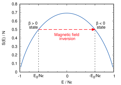
Figure 2: Entropy vs energy for the spin system (32) in the case of $1/2$ spins (two levels). Here $\varepsilon=\hbar\gamma|\mathbf{B}|/2$. The effect of a sudden inversion of the external magnetic field, as that performed in the experiments discussed in the main text, is qualitatively represented by the red arrow.

These concepts were discussed theoretically in the pioneering work by Ramsey ramsey56 , which represents the first systematic attempt to generalize equilibrium thermodynamics to negative temperatures states. The essential requirements identified by Ramsey and further justified by Klein klein56 for the existence of negative-temperature states are:

1. the system must be in thermodynamical equilibrium so that a proper temperature can be introduced to characterize its thermodynamic state;

2. the possible energy of the allowed states of the system must be bounded;

3. the system must be thermally isolated from all other systems which do not satisfy conditions (1) and (2).

Ramsey also mentions that in order to consider negative temperature, Kelvin-Planck formulation of the second law of thermodynamics needs to be modified in the following way:

It is impossible to construct an engine that will operate in a closed cycle and produce no effect other than (1) the extraction of heat from a positive temperature reservoir with the performance of an equivalent amount of work or (2) the rejection of heat into a negative-temperature reservoir with the corresponding work being done on the engine.

The reason of the above formulation can be easily understood by looking at Fig. 2. As long as the system is in the positive-temperature regime, extracting heat from it results in a decrease of its entropy; if such energy was completely converted into work, the total entropy would decrease too, leading to a paradox. Similarly, in the negative-temperature regime adding energy to the system by mean of mechanical work would result in a global decrease of entropy, and therefore this process is forbidden. This topic will be further discussed in Section III.3.3 of the present review.

It should be stressed that the emergence of negative temperatures in spin systems is not limited to paramagnetic systems. More recent experiments have demonstrated the existence of negative temperature states also in the presence of dominating ferromagnetic/antiferromagnetic interactions. An important example is the case of silver in cryogenic conditions hakonen92 , whose nuclear Hamiltonian can be approximated by

$$\mathcal{H}=-\sum_{\langle j,k\rangle}J_{jk}\mathbf{I}_{j}\cdot\mathbf{I}_{k}-\hbar\gamma\mathbf{B}\cdot\sum_{j=1}^{N}\mathbf{I}_{j}$$ (33)

where the (negative) coupling constants $J_{jk}$ identify a nearest-neighbor antiferromagnetic interaction. Here, equilibrium negative temperatures are signaled by the change of the sign of the interaction energy. Indeed, susceptibility measurements confirm the presence of ferromagnetic domains, which would be unstable at positive temperatures hakonen92 . The emergence of macroscopic ferromagnetic order from microscopic antiferromagnetic interactions is a relevant example of the physical significance of negative temperatures in spin systems.

II.3 Laser systems

Population inversions play a fundamental role in the physics of laser systems schawlow58 . The simplest example of a two-level laser discussed by Machlup machlup75 clarifies that this condition, applied to open systems, implies negative power absorption, i.e. power emission. Let indeed consider such a system where the quantum state “0” is the ground state with energy $E_{0}$ and the state “1” is the excited state with energy $E_{1}$. Let $h\nu=(E_{1}-E_{0})$ be the (positive) energy difference between the two levels, where $h$ is the Planck constant. Here we focus on a steady nonequilibrium process where the system is coupled to an external electromagnetic field. The rate of absorption $\mathcal{P}$ of energy from the field reads

$$\mathcal{P}=h\nu(w_{0\rightarrow 1}N_{0}-w_{1\rightarrow 0}N_{1})$$ (34)

where $w_{0\rightarrow 1}$ and $w_{1\rightarrow 0}$ are the induced transition rates between the two levels while $N_{0}$ and $N_{1}$ are the number of atoms in the lower and higher state, respectively. Time-reversal invariance implies that induced transition probabilities are symmetrical, i.e. $w_{0\rightarrow 1}=w_{1\rightarrow 0}=w$ yariv89 . Therefore, the absorption rate simplifies to $\mathcal{P}=h\nu w(N_{0}-N_{1})$. Accordingly, when a population inversion is steadily sustained in the system, i.e. when $N_{1}>N_{0}$, a power emission occurs.

The concept of negative absorption is central in the history of the development of laser systems and dates back to the results by Kramers kramers24 and the early experiments by Ladenburg and coworkers on an electrically excited Neon gas kopfermann28 . It is important to note that the occurrence of population inversions in steady nonequilibrium regimes can not be related to a global negative temperature in the sense of equilibrium thermodynamics (see first point of Ramsey’s requirements in Section II.2) machlup75 . If a local equilibrium hypothesis is verified, a negative temperature can be defined to characterize population inversions in a small but still macroscopic portion of the system lepri03 (see also Section VII). Nevertheless, population inversions may occur even in the absence of local equilibrium, when no proper temperature is well defined.

Several techniques to obtain population inversions and negative-temperature states were proposed and tested. Among the main mechanisms, it was discovered that in a three-level system with unequally spaced energy levels $E_{3}>E_{2}>E_{1}$, a large saturating field at frequency $(E_{3}-E_{1})/h$ can induce a population inversion in the pairs of levels $(3,2)$ or $(2,1)$ bloembergen56 . Other examples included the use of electric discharges sanders59 ; javan59 or rapid gas expansions basov63 . In the case of semiconductor lasers chow99 , Basov discusses in his Nobel lecture basov65 three different methods, namely:(i) optical pumping by means of an exciting field shined one the sample, (ii) creation of electron-hole pairs through beams of fast electrons, (iii) injection of electrons and holes through p-n junctions.

II.4 Cold atoms in optical lattices

In the last decades, the physics of cold atoms in optical lattices has become a prominent topic of investigation, with important applications in quantum control haycock00 and quantum computation brennen99 ; pachos03 . They also represent the ideal set-up for the study of quantum phase transitions greiner02 ; simon11 and many-body localization schreiber15 ; kaufman16 , as well as of the interplay between nonlinearity, discreteness and disorder in low-dimensional quantum systems fallani07 ; franzosi11 . Optical lattices jessen96 are obtained by interference patterns of counter-propagating laser beams which produce a stable and spatially periodic external potential for neutral atoms. This technique can be used to confine cold atoms in the wells of the optical potential and to make them experience a quantum tunneling effect between neighboring wells, with a resulting frequency spectrum characterized by bands. In particular, it can be shown that the quantum dynamics of a system of bosonic atoms in an optical lattice is described by a Bose-Hubbard model jaksch98 ; franzosi11 .

In this context, Mosk observed that the combination of a band gap and of a negative effective band curvature (aka negative band mass) could satisfy the requirements for thermalization of the gas at negative temperatures mosk05 . In analogy with early experiments on magnetic systems (see Section II.2), this peculiar thermalization process requires that the typical time scales for energy recombination are much faster than energy losses. More precisely, it is necessary that the selected band with negative effective mass displays a reduced rate of interband scattering processes, which provide an effective mechanism of energy dissipation towards different bands mosk05 .

Let us analyze more in detail this mechanism of thermalization at negative temperature in the framework of the Bose-Hubbard model gersch63 for an optical lattice with $N$ sites. The quantum many-body Hamiltonian operator reads

$$\hat{\mathcal{H}}=\frac{1}{2}U\sum_{j=1}^{N}\hat{n}_{j}(\hat{n}_{j}-1)-J\sum_{\langle jk\rangle}\left(\hat{a}_{j}^{\dagger}\hat{a}_{k}+\mbox{h.c.}\right)+\sum_{j=1}^{N}V(\mathbf{x}_{j})\hat{n}_{j}$$ (35)

where $\hat{a}_{j}^{\dagger}$ and $\hat{a}_{j}$ are bosonic creation and annihilation operators for an atom on lattice site $j$, satisfying standard commutation relations $[\hat{a}_{j},\hat{a}_{k}^{\dagger}]=\delta_{j,k}$, and $\hat{n}_{j}=\hat{a}_{j}^{\dagger}\hat{a}_{j}$ is the number operator for site $j$. The first sum in $\hat{\mathcal{H}}$ accounts effectively for the interactions of atoms in the same lattice well and is modulated by the parameter $U$, whose sign is determined by the attractive or repulsive nature of atom interactions. The second contribution, proportional to $J$, represents the hopping energy between nearest neighbor sites $\langle jk\rangle$. Finally, the last sum describes the contribution of an external trapping potential $V(\mathbf{x}_{j})$ (a magnetic trap), in the form of shifts of local site energies. In the following, we shall specialize $V(\mathbf{x})$ to the case of an harmonic trapping potential $V(\mathbf{x})=V_{0}|\mathbf{x}|^{2}$.

Let us assume that the parameters $U$ and $V_{0}$ are tunable, in such a way that they can assume both positive and negative values. The procedure proposed by Mosk mosk05 and later improved by Rapp, Mandt and Rosch rapp10 essentially consists of preparing an ultracold atomic gas with repulsive interactions ($U>0$) in an optical lattice with confinement $V_{0}>0$. In this configuration, the atomic system can be assumed in equilibrium at positive temperature. The height of the optical lattice potential is then increased such that $U/J\gg 1$. The system enters a deep Mott-insulator phase, which inhibits any transition between different lattice sites and “freezes” the gas in its initial state. The signs of $V_{0}$ and $U$ are then rapidly changed with no entropy variation and finally the intensity of the laser beams is lowered again as to bring $U/J$ to its original value. Basically, this protocol inverts the sign of the effective masses of the occupied states, operating a sort of controlled “population inversion”: in the equilibrium state that is reached, the new temperature is negative, the inter-particle potential is attractive ($U<0$) and the cloud of cold atoms is confined by the harmonic potential with $V_{0}<0$ rapp12 ; rapp13 ; mandt13 . The change of sign of the interaction term $U$ can be realized by tuning the magnetic bias near a Feshbach resonance feshbach62 ; inouye98 .

The above described NAT state was actually realized in a famous experiment on cold atoms by Braun et al. braun13 in 2013. The authors used a Bose-Einstein condensate of ³⁹K atoms in a 3-dimensional simple-cubic optical lattice. At the end of the experimental protocol, the momentum distribution of the atomic cloud was probed by mean of time-of-flight imaging kastberg95 , i.e. measuring the spatial spreading of the cloud during a small time interval (7 ms); in this way it was possible to verify that the distribution was peaked at the borders of the Brillouin zone, corresponding to maximal kinetic energy, as expected for a NAT state. The density of states was also in optimal agreement with the expected negative-temperature Bose-Einstein distribution. The equilibrium state, for optimized choices of the experimental parameters, was found to last for times of the order of hundreds of milliseconds (before decaying due to energy and atom losses), i.e. much longer than the typical lattice tunneling time. These experimental results are therefore a convincing evidence of the possibility to realize equilibrium thermodynamic states at negative temperature also for motional degrees of freedom.

Unlike point vortices and spin systems, whose energy does not include any contribution from motional degrees of freedom, a negative effective mass provides an efficient mechanism for bounding kinetic energies from above. Otherwise, the presence of a standard positive-definite kinetic term would forbid negative temperatures, since the phase-space region accessible to motional degrees of freedom would increase with the total energy, due to the quadratic dependence on momenta, see Sec. I.3. From a more general point of view, we point out that the experimental protocol here discussed amounts essentially to an inversion of the sign the total Hamiltonian operator of the trapped gas. This operation is analogous to the one performed in paramagnetic systems in the early experiments by Purcell and Pound purcell51 by means of a magnetic field inversion. We conclude this subsection by noting that also genuinely dynamical effects, usually related to nonlinearities, can contribute to restrict the accessible phase-space and produce NAT states. We will discuss this point in Sec. VI.1 in the context of the Discrete Nonlinear Schrödinger Equation.

II.5 Discrete Nonlinear Schrödinger Equation

The Discrete Nonlinear Schrödinger (DNLS) equation describes a simple model of a nonlinear lattice of coupled oscillators Eilbeck85 ; Kevrekidis09 . For a one-dimensional chain with nearest neighbor interactions, it can be written as

$$i\dot{z}_{j}=-\Lambda|z_{j}|^{2}z_{j}-z_{j+1}-z_{j-1}\,,\quad j=1,\cdots,N$$ (36)

where $z_{j}$ are complex-valued amplitudes and $\Lambda$ is a nonlinear coefficient. Unless otherwise specified, throughout this paper $\Lambda$ will be assumed positive without any loss of generality.

Since the pioneering investigations of the 50’s, the DNLS equation has been widely studied in several domains of physics. It was firstly derived by Holstein holstein59 within a tight-binding approximation for the motion of polarons in molecular crystals and later introduced in the context of the Davydov’s theory to describe energy transfer mechanisms in proteins davydov73 . Its novelty was immediately noticed as, unlike the continuous nonlinear Schrödinger and the Ablowitz-Ladik equation ablowitz76 ; scott03 , it is a nonintegrable model. Rapidly, it became clear that the DNLS equation and its generalizations including high-order weinstein99 or saturable khare05 nonlinearities or nonlocal interactions kevrekidis03 deserved great attention for the peculiar properties of its chaotic trajectories and periodic orbits Eilbeck03 . Indeed, this model is of particular interest for the study of discrete breather solutions, i.e. nonlinear and spatially localized excitations characterized by periodic oscillations in time flach98 ; flach08 and it has become a prototype model of nonlinear lattice dynamics Kevrekidis09 .

In addition to its theoretical interest, the DNLS equation is also representative model of nonlinear wave transport in a broad range of experimentally accessible setups Kevrekidis09 . These include nonlinear optical waveguide arrays christodoulides88 ; eisenberg98 ; morandotti99 , cold atoms in optical lattices smerzi97 ; trombettoni01 ; cataliotti01 ; cataliotti03 , electric transmission lines sato07 and nanomagnetic systems borlenghi14 ; borlenghi15 .

The statistical mechanics of the DNLS model was discussed in 2000 by Rasmussen et al. within the grand-canonical ensemble rasmussen00 . A Gibbsian measure was introduced which takes into account the two conserved quantities of the model, namely the total energy

$$H=\sum_{j=1}^{N}\frac{\Lambda}{2}|z_{j}|^{4}+\left(z_{j}^{*}z_{j+1}+c.c.\right)$$ (37)

and the total norm

$$A=\sum_{j=1}^{N}|z_{j}|^{2}\,.$$ (38)

Accordingly, the resulting equilibrium phase diagram is two-dimensional and it can be represented in the space of densities $(a,h)$, where $a=A/N$ is the average norm density and $h=H/N$ is the average energy density, see Fig. 3. In this diagram, the ground state of the model ($T=0^{+}$) is identified by the condition $h=\Lambda a^{2}/2-2a$. States below this line are not accessible and belong to the forbidden region $\mathrm{R_{f}}$. Moreover, the limit of diverging temperatures ($\beta=0$) defines the line $\mathcal{C}_{\infty}$, $h=\Lambda a^{2}$. Accordingly, positive-temperature states are confined in the region $\mathrm{R_{p}}$ between $\mathcal{C}_{0}$ and $\mathcal{C}_{\infty}$. Negative-temperature states were conjectured to exist in the region $\mathrm{R_{n}}$ above the infinite temperature line, although a direct treatment was impossible because of the ill definiteness of the grand-canonical measure in $\mathrm{R_{n}}$ rasmussen00 .

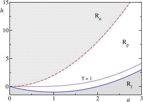
Figure 3: Equilibrium phase diagram $(a,h)$ of the DNLS equation for $\Lambda=2$. We show the isothermal lines $T=0$ (solid blue), $T=1$ (solid purple) and $\beta=0$ (dashed red).

In successive papers, it was shown that negative-temperature states in the DNLS equation are metastable and that in the thermodynamic limit the system eventually relaxes to an equilibrium state characterized by a single breather excitation superposed to an infinite-temperature background RN ; R1 ; R2 ; R3 ; R4 .

In parallel, the nature of the negative-temperature region has been extensively studied numerically. In particular, it was shown that the relaxation process can be extremely slow and that the system evolves towards a stationary state with a finite density of breathers and negative microcanonical temperature JR ; Iubini13 . This apparent contradiction with the theoretical predictions was clarified in Iubini14 ; Iubini17 ; ICOPP by pointing out two different sources of slowness. On the one hand localization occurs via a slow coarsening of breathers. On the other hand, the large oscillation frequency of a breather state tends to decouple it from the rest of the system, so that the observed timescales for breather-background norm transfer are exponentially long in the breather norm ICOPP . As a result the asymptotic convergence to the single-breather equilibrium state can be practically unattainable. In addition to the above phenomena, the equilibrium properties of the model in the $\mathrm{R_{n}}$ region have been recently reconsidered in the framework of large deviation theory GILM1 , finding that negative temperature states do exist as genuine equilibrium states for finite but large system sizes.

The DNLS equation has recently used as a prototypical model to study the role of negative-temperature states and localization in out-of-equilibrium contexts iubini17entropy . In particular, it was shown that a DNLS chain in contact with a reservoir at positive temperature and a pure norm dissipator reaches a partially localized nonequilibrium steady state where negative temperatures are spontaneously created. This phenomenon brings to the fore several aspects of the role of negative-temperature states in non-equilibrium statistical mechanics. Some of these points will be discussed in Sections VI, VII.

We conclude this section by observing that in the limit of vanishing nonlinearity, $\Lambda\rightarrow 0$, the DNLS equation reduces to a standard Schrödinger equation on a lattice. The thermodynamics of this model resembles the behavior of the class of paramagnetic systems discussed by Ramsey and implies the existence of a genuine negative-temperature region where no condensation occurs iubini19b ; buonsante16 (see also Section IV.3.1).

III Alternative interpretations

All physical systems described in Section II admit long-lasting states at high energy, whose statistical properties are conveniently portrayed by an equilibrium description at negative absolute temperatures. While no doubts are usually raised about the aforementioned experimental observations, their theoretical interpretation as thermal equilibrium states at negative temperature has raised some concern and criticisms, for different reasons. First, the very definition of temperature given in Section I.2 has been questioned by some authors berdichevsky91 ; hilbert14 ; sokolov14 ; hanggi15 ; campisi15 , claiming that the definition of absolute temperature usually adopted in statistical mechanics does not properly reproduce the basic principles of thermodynamics, and should be replaced by a different one, which does not admit negative values. Other authors criticize the description of the physical states observed in experiments as genuine equilibrium states, and point out the occurrence of paradoxical results for thermodynamic cycles romero13 ; struchtrup18 . In this Section we first discuss the alternative statistical description proposed by the authors who oppose to the traditional one; then we review the main contributions to the (still ongoing) debate about negative temperatures.

III.1 Two definitions of entropy (and temperature)

As discussed in Section I.2, the link between mechanics and thermodynamics is given by the formula

$$S(E)=k_{B}\ln W\,,$$ (39)

where, in Boltzmann’s picture, $W$ is the number of different, equiprobable states that the system is allowed to assume along its dynamics at fixed energy $E$, given a proper discretization of the phase-space. A precise mathematical expression of $W$ is available for any system of $N$ particles described by a Hamiltonian $\mathcal{H}({\bf Q},{\bf P})$, being ${\bf Q}\in\mathbb{R}^{dN}$ and ${\bf P}\in\mathbb{R}^{dN}$ the canonical positions and momenta in a $d$-dimensional space: one just exploits the proportionality between $W(E)$ and the density of states $\omega(E)$,

$$W(E)=\epsilon\omega(E)\,$$ (40)

leading to Eq. (39). It has been pointed out hilbert14 that Eq. (2) is – strictly speaking – not consistent from a dimensional point of view, since the argument of the logarithm should be dimensionless. For this reason, some authors prefer to keep the multiplicative factor $\epsilon$ inside the logarithm, with the physical meaning of the uncertainty associated with the measurement of $E$ (which is non-vanishing, due to Heisenberg’s uncertainty principle, in every physical system). Of course the particular choice of $\epsilon$ does not affect any measurable quantity, since it results in an unessential additive correction to the entropy.

An alternative definition of entropy can be found in a seminal work by J. W. Gibbs gibbs02 , later adopted also by Hertz hertz10 . The idea is to define $W(E)$ as the number of states in the phase-space volume enclosed by the hypersurface at constant energy $E$, instead of those on the hypersurface. In other words, one can define the quantity

$$\Sigma(E)=\int\mathcal{D}\mathbf{Q}\mathcal{D}\mathbf{P}\,\Theta\left(E-\mathcal{H}(\mathbf{Q},\mathbf{P})\right)\,,$$ (41)

$\Theta$ being the Heaviside function, and the corresponding Gibbs entropy:

$$S_{G}(E,N)=k_{B}\ln\Sigma(E,N)\,.$$ (42)

Note that $\Sigma(E)$ and the density of states verify the relation

$$\omega(E)=\frac{\partial\Sigma}{\partial E}\,.$$ (43)

Sometimes Boltzmann entropy, $S_{B}$, is also called surface entropy, while Gibbs’ one is referred to as volume entropy. The above volume entropy can be used to define, in a natural way, the so-called “Gibbs temperature” $T_{G}$:

$$\frac{1}{T_{G}}=\frac{\partial S_{G}(E,N)}{\partial E}\,.$$ (44)

In Section III.2 we shall recall that this quantity is characterized by very interesting properties.

It is important to recognize that in most physical situations $S_{B}$ and $S_{G}$ are equivalent, as soon as the thermodynamic limit $N\gg 1$ is considered huang88 . For instance, it is easy to verify that for a ideal gas of $N$ particle with mass $m$ in a $d-$dimensional space,

$$\Sigma(E)=c(2mE)^{Nd/2}$$ (45)

and

$$\omega(E)=cmNd(2mE)^{Nd/2-1}$$ (46)

where $c=\pi^{Nd/2}/\Gamma(Nd/2+1)$, so that the difference between Gibbs and Boltzmann entropy,

$$S^{id}_{G}(E)-S^{id}_{B}(E)=\ln\left(\frac{2E}{Nd}\right)$$ (47)

is subextensive, and it can be neglected in the thermodynamic limit.

III.2 Main properties of Gibbs’ formalism

Due to the equivalence between $T_{B}$ and $T_{G}$ for most physical systems, usually it is not so important to specify whether the temperature appearing in a formula comes from the Boltzmann’s formalism or from the Gibbs’ one: the relative difference is of order $N^{-1}$, i.e. it is negligible to any practical purpose. Conversely, when dealing with systems with bounded spectrum, as those discussed in Section II, one has to bear in mind that $T_{B}$ and $T_{G}$ can assume very different values: indeed, for such systems it is possible to find some energy regime in which $\omega(E)$ is a decreasing function of $E$, resulting in negative values of $T_{B}$; on the other hand, $\Sigma(E)$ is monotonically increasing, by definition, and therefore $T_{G}$ is always positive. It is then crucial to distinguish between the two alternatives.

As we will widely discuss in the next Sections, most results of Statistical Mechanics are expressed in terms of $S_{B}$ and $T_{B}$; these relations still hold true when $T_{B}$ assumes negative values, leading sometimes to counterintuitive effects, which can be actually observed in experiments or numerical simulations. There are, however, also some classical results which are derived in the Gibbs’ formalism, so that temperature and entropy appearing in the formulae have to be intended as $T_{G}$ and $S_{G}$ in these cases. This is a serious limitation if Gibbs’ and Boltzmann’s formalisms are not equivalent, as it happens for the kind of systems presented in Section II: as we shall discuss in Section IV, $T_{G}$ and $S_{G}$ cannot be easily measured in experiments, and the mentioned results have therefore little practical relevance. In the following we recall the main results involving $S_{G}$ and $T_{G}$.

III.2.1 Equipartition theorem

A useful result of statistical mechanics is the so-called “Equipartition theorem”, which states that, given a Hamiltonian system $\mathcal{H}(\mathbf{Q},\mathbf{P})$, the following relation holds:

$$\left\langle x_{i}\frac{\partial\mathcal{H}}{\partial x_{i}}\right\rangle=k_{B}T\,,$$ (48)

where $x_{i}$ is a certain canonical coordinate and $\langle\cdot\rangle$ denotes a microcanonical average. If $\mathcal{H}(\mathbf{Q},\mathbf{P})$ depends quadratically on the momenta, Eq. (48) implies that energy is equally distributed, on average, among the different kinetic degrees of freedom, hence the name of the theorem.

In deriving such result (see e.g. Ref. huang88 ) one makes use of Gibbs’ definition of entropy; consequently, Eq. (48) is exactly verified only if one interprets $T$ as $T_{G}$. See also Ref. dunkel14 on this point.

III.2.2 Exact validity of the Thermodynamic Relations

In thermodynamics, energy conservation is expressed by the First Law, which describes the energetic balance of a physical system subjected to external forces and/or thermal coupling with the environment, during an infinitesimal thermodynamic transformation. First Law can be expressed as

$$dE=\delta Q+dW\,,$$ (49)

where $dE$ is the total amount of energy acquired by the system during the transformation, given by the sum of the absorbed heat $\delta Q$ and of the work $dW$ which the system is subjected to. This infinitesimal work is due to the action of external thermodynamic forces, e.g. pressure or magnetic field, resulting in infinitesimal variations of macroscopic parameters of the system, such as volume or magnetization. In the following, we shall indicate the $n$ external forces acting on the system as $a_{1},a_{2},...,a_{n}$, and we shall refer to the corresponding macroscopic parameters as $A_{1},A_{2},...,A_{n}$. In formulae we have, by definition,

$$dW=-\sum_{j=1}^{n}a_{j}dA_{j}\,.$$ (50)

It is a phenomenological result of thermodynamics that a state function $S(E,A_{1},...,A_{n})$, the thermodynamic entropy, exists such that

$$\delta Q=TdS\,,$$ (51)

as far as reversible transformations are considered. The First Law can then be expressed as

$$dE=-\sum_{j=1}^{n}a_{j}dA_{j}+TdS\,.$$ (52)

As a consequence of the existence of the thermodynamic entropy we have that

$$\frac{1}{T}=\frac{\partial S}{\partial E}\,,$$ (53)

as it can be deduced from Eq. (52) in the case of a reversible transformation with fixed $\{A_{j}\}$. Similarly, if we consider an infinitesimal transformation in which only $A_{j}$ is varied, and such that energy remains constant, we have

$$\frac{a_{j}}{T}=\frac{\partial S}{\partial A_{j}}\,.$$ (54)

Equations (53) and (54) are often referred to as Thermodynamic Relations.

In order to give a statistical mechanics interpretation of the above experimental findings, one usually identifies the thermodynamic potentials with microcanonical averages of suitable mechanical observables. Let us denote by $\mathcal{H}(\mathbf{Q},\mathbf{P};A_{1},...A_{n})$ the Hamiltonian of the system, so that we can express work as

$$dW=\sum_{j}\left\langle\frac{\partial\mathcal{H}}{\partial A_{j}}\right\rangle dA_{j}\,,$$ (55)

where $\langle\cdot\rangle$, under the assumption of ergodicity, is an average on the microcanonical ensemble. Let us just mention that, according to the definition introduced by Jarzynski in Ref. jarzynski07 , we are considering here the inclusive definition of work. By comparing Eq. (50) and Eq. (55), one deduces

$$a_{j}=-\left\langle\frac{\partial\mathcal{H}}{\partial A_{j}}\right\rangle\,\quad\quad\forall j.$$ (56)

It can be shown campisi15 that Eq. (53) and (54) are verified exactly, also for a small number of particles $N$, only if the entropy $S$ is a function of $\Sigma(E)$ (the phase-space volume defined by Eq. (41)), i.e. only if

$$S(E)=g[\Sigma(E)]\,,$$ (57)

for some, sufficiently regular, $g:\mathbb{R}\mapsto\mathbb{R}$. Indeed, if this is the case, Eq. (54) can be written as

$$\frac{a_{j}}{T}=g^{\prime}(\Sigma)\frac{\partial\Sigma}{\partial A_{j}}\,,$$ (58)

which, by taking into account Eq. (56), leads to

$$Tg^{\prime}(\Sigma)\frac{\partial\Sigma}{\partial A_{j}} =-\frac{1}{\omega}\int\mathcal{D}\mathbf{Q}\,\mathcal{D}\mathbf{P}\,\delta(E-\mathcal{H})\frac{\partial\mathcal{H}}{\partial A_{j}}$$ (59)

$$=\frac{1}{\omega}\frac{\partial}{\partial A_{j}}\int\mathcal{D}\mathbf{Q}\,\mathcal{D}\mathbf{P}\,\Theta(E-\mathcal{H})$$

$$=\frac{1}{\omega}\frac{\partial\Sigma}{\partial A_{j}}\,.$$

This result is clearly consistent with Eq. (53):

$$\frac{1}{T}=g^{\prime}(\Sigma)\omega=\frac{\partial S}{\partial E}\,.$$ (60)

The simultaneous validity of Eqs. (53) and (54) is only guaranteed if $S(E)$ has the form (57). The particular choice $g(\Sigma)=\Sigma$ corresponds to Gibbs’ definition of entropy. It can be deduced, for instance, from the specific case of the ideal gas campisi15 .

III.2.3 Adiabatic invariance of the entropy

Making reference to the notation introduced in the previous paragraph, suppose now that parameters $\{A_{j}\}$ are time-dependent, and that the protocol which rules their evolution has a typical time $\tau$. The total energy $E$ is, in general, not conserved. If $\tau$ is very large, i.e. the transformation of the macroscopic parameters $\{A_{j}\}$ is very slow, the process is called adiabatic in the mechanical sense. A function $I(E(t);\{A_{j}(t)\})$, depending on the total energy of the system and on the macroscopic parameters, is called adiabatic invariant if

$$\lim_{\tau\to\infty}I(E(t);\{A_{j}(t)\})-I(E(0);\{A_{j}(0)\})=0\quad\quad\forall t:\quad 0\leq t<\tau$$ (61)

i.e. if its evolution can be approximated by a constant behavior in the interval $[0,\tau)$ when the characteristic time $\tau$ of the evolution is sufficiently large.

One of the assumptions of thermodynamics is that a very slow change of the parameters $\{A_{j}\}$ will result in a thermodynamic transformation in which no heat is exchanged between the system and the environment; in other words, it is generally believed that an adiabatic process in the mechanical sense should be also adiabatic in the thermodynamic sense campisi05 . This condition can be implemented by imposing that

$$\lim_{\tau\to\infty}\frac{dE}{dt}+\sum_{j=1}^{n}a_{j}\frac{dA_{j}}{dt}=0\quad\quad\forall t:\quad 0\leq t<\tau\,,$$ (62)

meaning that in the infinite $\tau$ limit the energy variation is only due to the work done on the system by the external forces. This is only true if $S$ verifies

$$\lim_{\tau\to\infty}\frac{dS}{dt}=0\quad\quad\forall t:\quad 0\leq t<\tau\,,$$ (63)

i.e. if $S$ is an adiabatic invariant in the mechanical sense campisi05 ; dunkel14 . It can be proved that $S_{G}$ possesses the above property, even for systems with a small number of degrees of freedom hertz10 ; kasuga61 ; berdichevsky97 . Conversely, in general $S_{B}$ does not verify this condition.

III.2.4 Helmholtz’s theorem

The last remarkable properties of Gibbs entropy (and temperature) that we discuss in this Section is maybe a little out of the scope of this review, since it only applies to systems with quadratic kinetic energy; it is the so-called “Helmholtz’s theorem”, a classical result providing a link between ergodicity and thermodynamics; this theorem had a crucial role in the development of Boltzmann’s ideas on statistical mechanics. This topic has been recently discussed by Gallavotti gallavotti13 and Campisi and Kobe campisi10 .

Consider a one-dimensional system with Hamiltonian

$$\mathcal{H}(q,p,V)=\frac{p^{2}}{2m}+\phi(q,V)$$ (64)

where $q$ and $p$ are the canonical coordinates, $m$ is the mass of the particle and $V$ is a control parameter, which can be varied. For instance, one may think to an oscillating pendulum, whose wire has a variable length $V$. These systems are called monocyclic. Assume that, for each value of $V$, the potential energy $\phi(q,V)$ has a unique minimum; assume also that, for $|q|\to\infty$, $\phi(q,V)$ diverges as $|q|$. In this system the motion is surely bounded once the value $E$ of the energy is fixed, i.e. it is possible to find suitable functions $q_{-}(E,V)$ and $q_{+}(E,V)$ of the external parameters such that

$$q_{-}(E,V)\leq q(t)\leq q_{+}(E,V)\,.$$ (65)

The motion is also periodic, with period $\tau(E,V)$. As a consequence, the system is ergodic in a trivial way: during its dynamics, the system explores all the states at energy $E$, so that the time averages coincide with the averages computed with the microcanonical distribution.

Let us now define the temperature $T$ and the pressure $P$ in terms of time averages $\langle\cdot\rangle_{\tau}$ computed on the period $\tau(E,V)$:

$$T \equiv{1\over k_{B}}\left\langle{p^{2}\over m}\right\rangle_{\tau}\,,$$ (66)

$$P \equiv-{1\over k_{B}}\left\langle{\partial\phi(q,V)\over\partial V}\right\rangle_{\tau}\,.$$

Let us notice that, according to the discussion in Section III.2.1, the above defined temperature is actually the Gibbs temperature $T_{G}$. The following result, due to Helmholtz, holds: the function

$$S(E,V)\equiv k_{B}\ln 2\int_{q_{-}{}}^{q_{+}}\sqrt{2m[E-\phi(q,V)]}dq=k_{B}\ln\int_{\mathcal{H}(q,p,V)<E}dpdq\,,$$ (67)

satisfies the following relations

$$\frac{\partial S}{\partial E} ={1\over T}$$ (68)

$$\frac{\partial S}{\partial V} ={P\over T}\,.$$

The above results imply a rather interesting consequence, namely that the quantity

$$dS=\frac{dE+PdV}{T}\,,$$ (69)

where $T$ and $P$ are expressed via time averages of mechanical observable, is an exact differential. $S$ can be then interpreted as a mechanical analogue of the thermodynamic entropy.

Boltzmann’s idea was to generalise the above result, valid for monocyclics, to systems with many particles; in other words he wanted to find a function $S(E,V)$ such that relations (68) and (69) are still valid. In a Hamiltonian system with $N$ particles, assuming ergodicity, it is indeed possible to prove a Generalised Helmholtz’s theorem campisi10 for the function

$$S(E,V)=k_{B}\ln\int_{H({\bf q},{\bf p},V)<E}\mathcal{D}{\bf Q}\mathcal{D}{\bf P}\,,$$ (70)

i.e. for the Gibbs entropy. As a consequence, the time averages can be replaced with the microcanonical averages, and from the Generalised Helmholtz’s theorem one can infer the Second Law of thermodynamics.

III.3 The debate about negative temperature

In the last years we have been facing a renewed dispute on the physical significance of negative temperatures, with different parties forming in the scientific community.

III.3.1 Critics of Boltzmann entropy

Dunkel and Hilbert dunkel14 , relying upon the assumption that thermostatistics can be derived from Gibbs entropy (along the lines of the discussion in Section III.2), concluded that negative temperatures are not compatible with this assumption. In particular, they contested the observation of negative temperature in motional degrees of freedom, claimed by Braun et al. in Ref. braun13 (see also Section II.4). This point of view was not completely new, since a similar position had been already expressed by Berdichevsky, Kunin and Hussain in Ref. berdichevsky91 . In that paper, the authors intended to criticize the use of a negative temperature formalism to refer to the high-energy regime of systems of vortices, as those described in Section II.1. In a more general perspective Hilbert, Hänggi and Dunkel hilbert14 argued that the zeroth, first and second principle of thermodynamics are fulfilled only by Gibbs entropy.

III.3.2 In defense of Boltzmann’s formalism and negative temperature

Frenkel and Warren frenkel15 showed that Gibbs entropy is conceptually inadequate, because it fails the basic principle (a direct consequence of zeroth law of thermodynamics, see Section IV.2) that two bodies at thermal equilibrium should be at the same temperature, at variance with the definition of entropy due to Boltzmann. These conclusions were further confirmed by the general approach due to Swendsen and Wang swendsen16 ; swendsen18 .

More recently, Abraham and Penrose abraham17 argued that the main argument raised against the negative temperature concept in the context of the Purcell and Pound experiment on nuclear spin systems purcell51 are not logically compelling. Moreover, they showed that the use of the so-called volume entropy leads to predictions inconsistent with the experimental evidence. We can say that in this paper the authors aim at providing clear answers to the main controversial points emerging from this dispute. In this sense, we consider Ref. abraham17 as an important reference for sketching the state of the art in this field.

A first aspect that is clarified in Ref. abraham17 is that the thermo-statistical consistency condition

$$TdS=\delta Q=dE-dW$$ (71)

which, for a magnetic system like the one of the Purcell-Pound experiment, specializes to $dW=-Mdh$ ($M$ being the magnetization and $h$ the external magnetic field) holds true also for the Boltzmann “surface” entropy and not only for the “volume” Gibbs entropy, at variance with what previously sustained by some authors (e.g., see berdichevsky91 ; dunkel14 ). In a more general perspective, it has been shown that if the averages appearing in Eq. (55) are interpreted as canonical ones (instead of microcanonical, as proposed in Ref dunkel14 ), the consistency criterion is always satisfied by Boltzmann entropy frenkel15 ; buonsante16 .

Another important point discussed by Abraham and Penrose concerns an experimental test of the different entropy formulas. They elaborate on the same conceptual direction raised by Frenkel and Warren frenkel15 and Swendsen and Wang swendsen16 that Gibbs’ entropy contradicts the zeroth law of thermodynamics, while making explicit reference to the experiment by Abragam and Proctor abragam57 ; abragam58 . In this old experiment two spin systems made of N nuclei of magnetic spin $\mu$ were brought into thermal contact and the question is if and how to eventually reach a thermal equilibrium state starting from a out-of-equlibrium initial condition, where one set of N nuclei is prepared at null energy and the other set of N nuclei is at maximal energy. Abraham and Penrose show that making use of Boltzmann entropy one can predict that the overall system will eventually evolve to an equilibrium state where the total initial energy is equally shared between the two spin systems, which is exactly what was observed in the experiments. But they also show that the adoption of the Gibbs entropy does not allow to predict that the energy equipartition state is eventually approached: the energy in the two subsystems, after being put in thermal contact, is allowed to perform a sort of random walk, characterized by arbitrary large fluctuation preventing the possibility of equipartition.

Finally, Abraham and Penrose comment about the possibility of designing superefficient Carnot engines, i.e. yielding $\eta>1$ from negative temperature sources, as asserted in braun13 ; ramsey56 . Making also reference to previous careful analyses frenkel15 ; landsberg77 , they definitely clarify that, when dealing with a Carnot engine exchanging heat with two sources at temperatures of different sign, one cannot rely upon the standard hypothesis of adiabatic transformations. Anyway, they also argue that one cannot overtake a Carnot efficiency $\eta=1$ and that such a situation may occur without contradicting any principle of thermodynamics, see Section III.3.3 below.

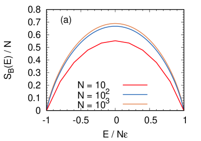
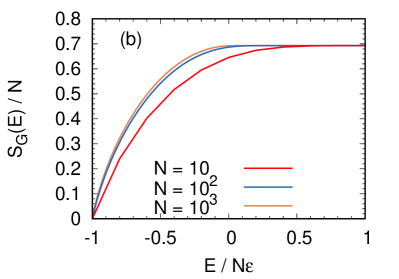
Figure 4: Entropy of the spin system 4, according (a) to the Boltzmann’s and (b) to the Gibbs’ definition, for different values of the number of particles $N$.

More arguments in favor of Boltzmann entropy can be found in other papers. For instance, in Ref. buonsante17 an example of phase transition at negative temperature is exhibited, which could not be characterized in the Gibbs’ formalism. In Ref. cerino15 it is shown that a correct description of thermodynamic fluctuations requires the use of Boltzmann temperature. In Ref.s vilar14 ; buonsante16 ; swendsen18 the scalings of $S_{G}$ and $T_{G}$ in the thermodynamic limit are analysed, and it is shown that they provide no useful information about the high-energy regime of models living in bounded phase-space. To clarify this point, let us consider again the simple spin model (32) introduced in Section II.2. For this system it is possible to compute explicit values for $S_{B}$ and $S_{G}$ for any fixed number of particles $N$, and the approach to the thermodynamic limit can be studied. Indeed, denoting by $N_{-}=(N+E/\varepsilon)/2$ the number of negative spins in a configuration with energy $E$, with $\varepsilon=\hbar\gamma|\mathbf{B}|/2$, the number of states corresponding to that energy is given by

$$W_{N_{-}}=\frac{N!}{N_{-}!(N-N_{-})!}\,,$$ (72)

so that

$$S_{B}=\ln W_{N_{-}}\,,\quad\quad S_{G}=\ln\sum_{n=0}^{N_{-}}W_{n}\,.$$ (73)

Both quantities are plotted in Fig. 4, for increasing values of $N$. As the thermodynamic limit is approached, Gibbs entropy tends to a plateau for $E>0$, i.e. for those values of the energy corresponding to negative temperatures in the Boltzmann description. As a consequence, Gibbs’ formalism does not allow for a proper thermodynamic description of the properties of such states, which are all identified by infinite temperature ($\beta=0$) in the limit of infinite $N$. See Section IV.3.1 for a wider discussion on this model.

III.3.3 The problem of thermodynamic cycles

The possibility to design a thermodynamic engine operating between two inverse temperatures $\beta_{1}$ and $\beta_{2}$ such that $\beta_{2}<\beta_{1}<0$, or even $\beta_{2}<0<\beta_{1}$, is another controversial point which has been being debated since the seminal paper by Ramsey ramsey56 . In that work it is mentioned that Carnot cycles can be designed for spins systems subject to an external field $\mathbf{B}$ which is continuously varied, at a very slow rate, so that the system can be considered in a thermal equilibrium condition at every time. This external parameter plays the role assumed by the volume in the case of ideal gases. In principle, we can perform reversible transformations at fixed temperature, positive or negative, as well as adiabatic transformations in which the system does not exchange heat with the environment. It is worth noticing that this is true both at positive and at negative temperature, provided that the sign of temperature does not change during the transformation. The efficiency of such a Carnot cycle is defined as

$$\eta=1-\frac{Q_{2}}{Q_{1}}=1-\frac{T_{2}}{T_{1}}$$ (74)

where $Q_{1}$ is the heat absorbed at temperature $T_{1}$ and $Q_{2}$ is that released at temperature $T_{2}$ (we are assuming that $T_{1}$ is hotter than $T_{2}$, i.e. we are either in the $0<T_{2}<T_{1}$ or in the $T_{2}<T_{1}<0$ case). As argued by Ramsey, the fact that for $T_{2}<T_{1}<0$ the efficiency can be negative, and even less than $-1$, means that work must be done on the system in order to maintain the cycle: this behavior is opposite to the positive-temperature case, in which the absorbed heat is converted into work by the engine. The whole picture is consistent with the “generalized” Kelvin-Planck formulation of the second law of thermodynamics, enunciated by Ramsey himself, stating that at negative temperature it is not possible to completely transform work into heat (whereas, at positive temperature, this process is allowed and the reverse one is forbidden, see Section II.2). In a later paper by Landsberg a precise correspondence is established between heat pumps at $T<0$ and heat engines at $T>0$ landsberg77 .

If $T_{1}$ and $T_{2}$ have different signs the scenario is a bit more involved. Ramsey noted that, for systems of nuclear spins, no way is known to operate adiabatic transformations between temperatures of opposite signs: indeed, as discussed in Section II.2, the experimental protocol that is adopted to achieve negative values of $\beta$ in magnetic systems rely on a non-quasistatic inversion of the external field. However it is not clear, a priori, whether an adiabatic transformation between positive and negative temperature is forbidden in any kind of physical system, or in spin systems only tykodi75 . An answer to this question was provided by Schöpf schopf62 : after systematically analysing all non-paradoxical thermodynamic cycles, i.e. those which do not contradict the first and the second law of thermodynamics, he concluded that every adiabatic transformation linking states at negative and positive temperature would result in some inconsistencies. In a subsequent work tykodi78 it has been shown that one of the proofs was incomplete, and that the third law of thermodynamics also needs to be assumed. A proof for the case with bounded energy is given in Ref. tremblay76 . Under reasonable hypotheses, it is shown that if one considers a thin enough region around the $\beta=0$ surface, in the state-variables space, entropy is constant, and maximal, at $\beta=0$. An immediate consequence is that such surface cannot be crossed by an isoentropic transformation.

While quasi-static Carnot cycles between temperatures with opposite signs are not allowed, their non-quasistatic versions can be still realised. A systematic discussion on this topic can be found in Ref. landsberg80 . The efficiency of such engines, according to Eq. (74), is larger than one, an apparently paradoxical result. The contradiction is solved by noticing that Eq. (74) is derived under the assumption that heat is absorbed by the system at temperature $T_{1}$ and released at temperature $T_{2}$, which is not possible if $T_{2}<0<T_{1}$ or $T_{1}<0<T_{2}$: in that case (as discussed in Ref. campisi16 ) heat is absorbed by both reservoirs and completely converted into work, so that the efficiency

$$\eta=\frac{W}{Q}$$ (75)

is actually always equal to 1. Obviously this does not mean that it is possible to completely convert an arbitrary large amount of heat into work: as correctly pointed out in Ref. frenkel15 ; struchtrup18 , the work needed in order to realize a negative-temperature bath largely exceeds the one that can be obtained in this way. Such cycles have been experimentally realised in quantum systems deassis19 .

III.3.4 Critics of negative-temperature equilibrium

In the light of all of these achievements one could have expected that the dispute might have come to a happy end. This is not exactly the case, because even more recently there was a revival, based on the criticism that negative temperature states are not true equilibrium states struchtrup18 , as assumed by Ramsey in his influential paper of 1956 ramsey56 . As recalled in Sec. I.3, if one wants to discuss about negative temperature states, one has to deal with an isolated thermodynamic system abraham17 . Indeed, any coupling with the external environment, which is composed by ordinary matter at positive temperature, would eventually lead to an equilibrium state at $T_{B}>0$, as already understood by Ramsey ramsey56 . See Section IV.2 for further discussion on this point. This is the reason why in all experiments on negative-temperature states it is crucial for the relaxation time of the system to be much smaller than the typical time-scales of the thermalization with the environment purcell51 ; pound51 ; braun13 .

Some authors claim that this is enough to consider states at NAT as out-of-equilibrium romero13 ; struchtrup18 . Of course this conclusion depends on which definition of “thermodynamic equilibrium” is chosen, but it does not affect the ability of equilibrium statistical mechanics to properly characterize the considered states (as discussed in Section IV in some detail).

III.3.5 Remarks

In summary, we believe that the main merit of this dispute is that it has re-raised the very long-standing problem about the equivalence of different definitions of entropy and their relevance and consistency with thermodynamics and related experimental facts. In fact, the kind of problems that have been selected as relevant by the statistical mechanics community in the last half a century could ignore the problem of its foundations, simply because any definition of entropy, either Gibbs’ or Boltzmann’s, yielded the same conclusions. Facing new questions about models with bounded energy spectra, long-range interactions and condensation phenomena has determined a drastic change of perspective, asking for crucial conceptual improvements in view of a consistent and physically sound theory of thermodynamic phenomena. By the way, it is important to mention that such a revision has to deal with other basic concepts like ergodicity. Anyway, we want to state clearly that the understanding of a physical phenomenon cannot depend on one’s favorite definition of entropy.

The above mentioned debate has suffered from taking a wrong perspective from the very beginning, when it was claimed that negative temperatures can be adopted as the right concept for referring to some peculiar physical phenomena. Actually, the ambiguity in defining temperature by the volume (i.e., Gibbs-like) or by the surface (i.e., Boltzmann-like) entropies is essentially irrelevant when compared with experimental facts. For instance, quite recent experimental achievements showed that the “negative temperature” regime predicted by the Onsager’s model of point vortices does exist, because of the special features of the interactions among such vortices gauthier19 ; johnstone19 .

Also in the light of these recent achievements, it seems to us that a general method to be adopted for identifying conditions corresponding to negative temperature phenomena has to based on the properties of the density of states $\omega(E)$ of a given isolated system described by a Hamiltonian, rather than by the ambiguous choice of the preferred entropy. Note that the density of states is not prone to any ambiguous interpretation, it is relevant for classical as well as for quantum systems and it allows one to establish the basic conditions to observe unusual thermodynamic behavior, irrespectively of the system at hand. For instance, in Sec. 1.3 we have already discussed how, looking at $\omega(E)$, one can easily conclude that Hamiltonian models with extensive standard kinetic energy cannot exhibit negative temperatures, and also why Hamiltonian models with bounded phase space have to. The models discussed in Sec. 2 belong to the latter class of systems, with the remarkable exception of the DNLS one (see Sec. 2.5). We want to point out here that for this model the presence of negative temperatures can rely upon Machlup’s criterion [29]: peculiar physical phenomena (i.e., negative temperatures) can be observed in systems where at infinite temperature the typical energy is finite, in formulae

$$\int_{0}^{+\infty}e^{-\beta E}E\omega(E)dE|_{\beta=0}=\int_{0}^{+\infty}E\omega(E)dE=\langle E\rangle_{0}<\infty$$ (76)

In particular, if the system can access values of $E$ larger than $\langle E\rangle_{0}$ we have to face a new kind of thermodynamic phenomena. It can be easily argued that condition (76) applies to the DNLS problem. In fact, as discussed in Sec. 2.5, for any fixed value of the conserved total norm $A$ one has $\langle E\rangle_{0}=2aA$. This result stems from two basic physical properties of the DNLS model: the hopping term is not a standard kinetic one (actually, on the line $\beta=0$ it is subextensive, because the phases of the complex state variables $z_{j}$ have to be random) and, beyond total energy $E$, it has an additional conserved extensive quantity $A$, because of the gauge symmetry $z_{j}\to e^{i\pi j}z_{j}$. In retrospect it is quite a peculiar fact that nowhere in the papers cited in Sec. 2.5 it was realized that it is would be enough to reconsider Machlup’s criterion for concluding that negative temperatures pertain the DNLS model, as well as systems with population inversion, for which it was originally formulated (see [29]). Note also that Machlup’s criterion (76) is a stronger bound than assuming that $\omega(E)$ is just a decreasing function of $E$, which, as already mentioned, is a sufficient criterion for negative temperatures, once Boltzmann entropy is taken as a suitable definition.

However, since $|\gamma|$ is usually proportional to the number of degrees of freedom of the system, we remark that that condition might be only realized in systems with very few particles.

To conclude this Section, let us stress once again that the existence of physical systems which show the high-energy behaviour identified by Machlup’s criterion (as those discussed in Section II) is an experimental fact; most authors (with some exceptions: see e.g. Ref. struchtrup18 ) agree that such systems, when isolated from the external environment, reach thermal equilibrium even if the energy $E$ of the system corresponds to a decreasing branch of the density of states $\omega(E)$. The choice between Boltzmann or Gibbs temperature is, of course, a matter of taste; however the former, for this kind of systems, has the practical advantage to assume opposite signs in presence of the two, qualitatively different, thermodynamic regimes. In our opinion, as already pointed out by Montgomery montgomery91 in a comment to Ref. berdichevsky91 , the last point provides a very good reason to choose Boltzmann’s formalism when dealing with systems satisfying Machlup’s criterion.

IV Equilibrium at $\beta<0$

In this Section we review some fundamental topics about the equilibrium statistical mechanics of systems which admit negative absolute temperatures. We aim at clarifying in which sense temperature is a physical observable, also for systems where no equipartition theorem is expected to hold, and how it is related to the statistical properties of the system. The problem of ensemble equivalence at negative temperature is discussed in some detail: even if, in principle, the possibility to achieve negative temperature does not imply a failure of ensemble equivalence, several relevant systems show both features. We investigate this link by considering some particular examples.

IV.1 The problem of measuring temperature

In Section I.2 we have recalled and justified the notion of temperature as it is usually meant in statistical mechanics. Since two alternative definitions of entropy are commonly used in literature, two distinct quantities with the meaning of temperature, $T_{B}$ and $T_{G}$, can be defined as well: as discussed in Section III.1, in the thermodynamic limit such observables assume nearly identical values for most physical systems, but they may show very dissimilar behaviours if the system lives in bounded phase space. From a physical point of view, a very important question to address is whether (and how) these quantities can be measured – at least in principle – in actual experiments or in numerical simulations. In other words, one would like to have a protocol to determine $T_{B}$ and $T_{G}$ by only sampling a system at equilibrium. In this Section we address this problem, devoting particular attention to models which admit NAT.

The temperature of a macroscopic object whose internal degrees of freedom are in thermal equilibrium is determined, in everyday practice as well as in experiments, by putting a measuring device (a thermometer) at contact with a small portion of the system. The thermometer has only access to information about the state of this small subsystem, which we can identify with a vector ${\bf X}\in\mathbb{R}^{2dN_{1}}$, where $N_{1}$ is much smaller than $2dN$, the dimension of the full phase space $({\bf Q},{\bf P})$. Let us also indicate with $\widetilde{{\bf X}}\in\mathbb{R}^{2d(N-N_{1})}$ the remaining variables. The Hamiltonian can be decomposed into

$$\mathcal{H}({\bf Q},{\bf P})=\mathcal{H}_{1}({\bf X})+\mathcal{H}_{2}(\widetilde{{\bf X}})+\mathcal{H}_{I}({\bf X},\widetilde{{\bf X}})$$ (77)

where $\mathcal{H}_{1}$ and $\mathcal{H}_{2}$ include all terms only depending on ${\bf X}$ and $\widetilde{{\bf X}}$ respectively, while $\mathcal{H}_{I}$ accounts for the interaction terms between the two subsystems. In the microcanonical ensemble, where the total energy is fixed to $E$, the probability density function (pdf) for the full phase space is

$$p({\bf Q},{\bf P})=\frac{1}{\omega(E,N)}\delta(\mathcal{H}({\bf Q},{\bf P})-E)\,.$$ (78)

Let us now specialize to the physically relevant case $1\ll N_{1}\ll N$. To determine the pdf $p_{1}({\bf X})$, which describes the stationary state of the subsystem “seen” by the thermometer, one has to marginalize $p({\bf Q},{\bf P})$ by integrating over the unaccessible variables $\widetilde{{\bf X}}$. The derivation is quite simple, and it can be found in many textbooks ma85 ; huang88 : assuming that $\mathcal{H}_{I}({\bf X},\widetilde{{\bf X}})$ is negligible with respect to $\mathcal{H}_{1}$ and $\mathcal{H}_{2}$, an hypothesis which can be rigorously proved if the system has short-range interactions campa09 , we have

$$p_{1}({\bf X})\simeq\frac{\omega_{2}(E-H_{1}({\bf X}),N-N_{1})}{\omega(E,N)}\,,$$ (79)

where $\omega_{2}$ is the density of states of the subsystem $\widetilde{\mathbf{X}}$. By writing $\omega$ in terms of $S_{B}$, the Boltzmann entropy defined by Eq. (4), we have

$$\omega(E,N)=e^{S_{B}(E,N)/k_{B}}$$ (80)

and

$$\omega_{2}(E-\mathcal{H}_{1}({\bf X}),N-N_{1})=e^{S_{B}(E-\mathcal{H}_{1}({\bf X}),N-N_{1})/k_{B}}\,.$$ (81)

Let us remark that in the previous equation the functional form of $\omega_{2}$ is assumed to be the same as that of $\omega$, which is a reasonable approximation in the limit $N_{1}\ll N$ even if the system is not homogeneous. Since $\mathcal{H}_{1}({\bf X})\ll E$, we can exploit the expansion

$$S_{B}(E-\mathcal{H}_{1}({\bf X}),N-N_{1})\simeq S_{B}(E)-\frac{\partial S_{B}(E,N)}{\partial E}\mathcal{H}_{1}({\bf X})+const\,.$$ (82)

Using equations (79, 81) and (82), together with the definition of Boltzmann (inverse) temperature (13), one obtains the pdf of the small subsystem

$$p_{1}({\bf X})=\frac{1}{Z_{\beta}}\,e^{-\beta H_{1}({\bf X})}\,,$$ (83)

$Z_{\beta}$ being a normalization factor. In other words, the thermometer has access to a portion of the system, whose state is described by a canonical distribution corresponding to the Boltzmann inverse temperature

$$\beta=\frac{\partial S_{B}}{\partial E}\,.$$ (84)

Since this temperature can be negative, there is no obstacle, in principle, to the design of a thermometer able to measure negative temperature, as we will show in the next section.

The above discussion can be also applied to the case in which $\mathbf{X}$ represents one degree of freedom only, for instance a “generalized” momentum of the Hamiltonian

$$\mathcal{H}=\sum_{n=1}^{N}\mathcal{K}(P_{n})+\mathcal{U}(\mathbf{Q})$$ (85)

where the variables $\{P_{n}\}$, as well as the functions $\mathcal{K}(P)$ and $\mathcal{U}(\mathbf{Q})$, are bounded. Using the same argument presented above, one obtains the generalised Maxwell-Boltzmann distribution:

$$\rho(P)\propto e^{-\beta\mathcal{K}(P)},$$ (86)

which is valid for both positive and negative $\beta$. The analysis of the momentum pdf can then be used as a practical recipe to measure both positive and negative Boltzmann temperatures in real experiments braun13 , as well as in numerical simulations.

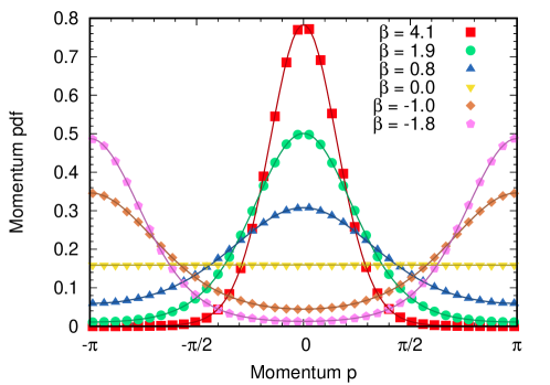
Figure 5: Single-particle momentum distribution for a model with bounded Hamiltonian. Points: histograms of $P$ obtained from molecular dynamics simulations of model (85) with kinetic energy (87) and potential (88), for different values of the total energy. Solid lines: best fit of the pdf with the functional form (86); the resulting values of $\beta$ are reported in the key. All simulations have been executed through a second order Velocity Verlet integration scheme with time step $\Delta t=10^{-3}$, over a total integration time (for each plot) of $\mathcal{T}=10^{5}$. Here $N=128$.

A minimal example is presented in Fig. 5, where the pdf of the single particle momentum $P$ is shown, for several values of $\beta$, in a Hamiltonian system of the form (85) with

$$\mathcal{K}(P)=1-\cos(P)$$ (87)

and

$$\mathcal{U}(\mathbf{Q})=\frac{1}{2}\sum_{n=1}^{N}[1-\cos(Q_{n}-Q_{n-1})]\quad\quad Q_{0}\equiv Q_{N}\equiv 0\,.$$ (88)

This model has been introduced in Ref. cerino15 as an example of Hamiltonian with bounded phase space; the peculiar form of the kinetic energy resembles the semi-classical limit of the bosonic system studied in Ref. braun13 and it has been investigated also in Ref. hanggi15 . In the low-energy limit the functional form of the kinetic terms tends to the usual one, $\mathcal{K}(P)\simeq P^{2}/2$, while the potential interaction reduces to that of a chain of harmonic oscillators; in this limit, the chain behaves as a classical Hamiltonian system at positive temperature, and $\rho(P)$ resembles the usual Gaussian distribution. The scenario is different at high energies: in this case, the dynamics typically selects configurations in which the angular distance between two neighbour oscillators is maximized cerino15 and the distribution of the momentum is peaked around $P\simeq\pi$ (see Fig. 5), a state corresponding to a negative value of $\beta$. The knowledge of the functional form of the pdf (86) allows to infer the value of the (Boltzmann) temperature through a fit over the distribution, even in cases with negative temperature.

An alternative way to measure the microcanonical Boltzmann temperature has been proposed by Rugh rugh97 ; rugh98 . It can be shown that $\beta$ is correctly estimated by the following observable:

$$\beta=\frac{1}{\omega(E)}\frac{\partial\omega(E)}{\partial E}=\left\langle\Phi\right\rangle_{E}$$ (89)

where

$$\Phi=\nabla\cdot\left(\frac{\nabla\mathcal{H}}{||\nabla\mathcal{H}||^{2}}\right)\,.$$ (90)

and the average is computed according to the microcanonical distribution, over the energy constant hypersurface $\Gamma_{E}=\{{\bf X}:\mathcal{H}({\bf X})=E\}$. A proof of the above result can be found in Ref. puglisi17 . The conceptual and practical relevance of formula (89) relies on the fact that it links temperature to a mechanical observable giardina98 ; since the considered average is microcanonical, one can compute temperature through a time average along a trajectory (assuming ergodicity):

$$\beta=\lim_{\cal T\to\infty}{1\over{\cal T}}\int_{0}^{\cal T}\Phi({\bf Q}(t),{\bf P}(t))\,dt\,.$$ (91)

If the system is very large ($N\gg 1$), Eq. (89) can be simplified in the following way puglisi17 :

$$\beta\simeq\left\langle{\nabla^{2}\mathcal{H}\over||\nabla\mathcal{H}||^{2}}\right>_{E}\Big{(}1+O\Big{(}{1\over N}\Big{)}\Big{)}\simeq{\left<\nabla^{2}\mathcal{H}\right\rangle_{E}\over\left<||\nabla\mathcal{H}||^{2}\right>_{E}}\Big{(}1+O\Big{(}{1\over N}\Big{)}\Big{)}\,.$$ (92)

If the Hamiltonian is quadratic, in the limit of large $N$ we recover an expression which is consistent with the equipartition theorem. Eq. (89) has been further generalised jepps00 ; rickayzen01 : it is possible to show that

$$\beta=\left<\nabla\cdot\Big{(}{{\bf B}\over{\bf B}\cdot\nabla\mathcal{H}}\Big{)}\right>_{E}$$ (93)

where ${\bf B}$ is a vector of arbitrary continuous and differentiable functions of the phase-space. Such a generalization has been successfully used in numerical simulations, for instance to check the algorithmic correctness of Monte Carlo computer programs, and to design new thermostats morriss99 ; jepps00 . Rugh’s approach may lead to particularly interesting equivalences for systems whose Hamiltonian structure is different from (85), as for instance the $2D$-model for inviscid hydrodynamics discussed in Section II.1. The result has been also extended to the case of one or more conserved quantities Franzosi ; franzosi12 . Let us also notice that from the microcanonical definition (90) it follows that a change of sign of $H$ implies a change of sign of $\beta$, and vice versa. This general property has profound implications also for experiments, as it corresponds to the main protocol employed to produce NAT states in purcell51 ; schreiber15 .

So far, we have shown that it is generally possible to measure the Boltzmann temperature, even if it assumes negative values, by studying the distribution of some degrees of freedom of the system or by looking at proper observables. Critics of Gibbs’ definition of entropy stress that $T_{G}$, on the contrary, is unphysical in the following sense: it is a function of a phase-space volume region which includes states that the system is not allowed to visit, because of energy conservation schneider14 ; buonsante17 . By looking at an actual trajectory of the system in the phase space one cannot sample such volume, the dynamics being constrained on the constant-energy hypersurface. The problem of measuring $T_{G}$ can be actually approached in an alternative way, often discussed in textbooks. As discussed in Section III.2.1, the Equipartition Theorem sets a link between a microcanonical average and the Gibbs temperature

$$\left\langle x_{i}\frac{\partial\mathcal{H}}{\partial x_{j}}\right\rangle_{E}=\delta_{ij}T_{G}\,;$$ (94)

again, if one assumes ergodicity, Eq. (94) allows to compute temperature by mean of time averages. However, it is important to notice that the usual derivation of Eq. (94) implies the possibility to neglect boundary terms in an integration by parts cerino15 ; buonsante16 . This possibility is challenged when the phase space is bounded, and in particular it can be shown that Equipartition Theorem does not hold under the simultaneous realization of the following conditions cerino15 :

1. bounded space of the canonical variables;

2. bounded derivatives of the Hamiltonian $\frac{\partial\mathcal{H}}{\partial x_{j}}$;

3. bounded energy from above and below: $E_{m}\leq E\leq E_{M}$;

4. vanishing density of states at the boundaries, i.e. $\omega(E_{M})=0$.

Given such conditions, one has that, on the one side, $T_{G}(E)={\Sigma(E)}/{\omega(E)}$ diverges when $E\to E_{M}$; on the other side, $\langle x_{i}\frac{\partial\mathcal{H}}{\partial x_{j}}\rangle$ is limited, resulting in a contradiction. In the light of the above, Eq. (94) can fail even in systems where there are no negative temperatures and $T_{G}\simeq T_{B}>0$ for all $E$. Consider, for instance, the following Hamiltonian

$$\mathcal{H}=\sum_{n=1}^{N}{p_{n}^{2}\over 2}+\epsilon\sum_{n=1}^{N}[1-\cos(q_{n}-q_{n-1})]$$ (95)

where $q_{n}\in[-\pi,\pi)$. For large $E$, i.e. $E\gg\epsilon N$, the contribution to $\Sigma(E)$ of the variables $\{q_{n}\}$ is almost independent of the value of $E$, so that $\Sigma_{\epsilon}(E)\simeq\Sigma_{0}(E)\propto\,E^{N/2}$, and $T_{G}\simeq 2E/N$. In the limit $N\gg 1$, we have that $T_{B}\simeq T_{G}+O(1/N)$; on the other hand it is easy to see that

$$\left|q_{n}{\partial\mathcal{H}\over\partial q_{n}}\right|\leq 2\pi\epsilon\,\,,$$ (96)

and, therefore, formula (94) cannot be valid for large values of $E$ and $N$.

IV.2 Zeroth law and thermometry

From a thermodynamic point of view the notion of temperature is based on the Zeroth Law: if two systems $\cal A$ and $\cal B$ are each at thermal equilibrium with a third, then they are at thermal equilibrium with each other. This implies that being at thermal equilibrium is an equivalence relation, and temperature is the thermodynamic quantity that determines to which “class of equivalence” a system belongs kardar07 ; puglisi17 . This principle justifies the usage of thermometers to measure temperature: it is sufficient to verify that $\cal A$ is at thermal equilibrium with a thermometer at a certain temperature to conclude that it belongs to the class of equilibrium identified by that temperature.

As mentioned in Section IV.1, in principle it is possible to use a thermometer to measure the temperature of systems with bounded phase space, even when $\beta<0$. However we know from the discussion in Section I.3 that coupling a system $\mathcal{A}$ at negative temperature with a system $\mathcal{B}$ composed by ordinary matter will lead after a certain time to an equilibrium state at positive temperature. Therefore if we try to use the system $\cal B$ as a thermometer to read the absolute temperature of $\cal A$, we shall observe the rather disappointing result that the thermometer heavily perturbs the measured system, changing the sign of its original temperature. The above result is in obvious disagreement with the natural idea that a thermometer should be able to measure a system’s temperature within an acceptable time and without perturbing it significantly. The above difficulty comes from the fact that once $\cal A$ and the thermometer are coupled together, the resulting system lives in a unbounded phase space, due to the degrees of freedom of the thermometer ramsey56 . The problem is solved as soon as the measuring device also admits NAT states: as shown in Ref. buonsante16 , if two systems admitting negative temperature are coupled together, they will eventually reach the same inverse Boltzmann temperature, whose value will be intermediate between the two $\beta$’s of the subsystems. In that work the Hamiltonian dynamics of systems inspired by a (quantum) bosonic dynamics is numerically simulated; in the following we shall discuss a similar numerical experiment on Hamiltonian systems with the generalized kinetic energy (87) introduced in the previous Section. Further details can be found in Ref. baldovin17 .

Let us consider (i) a sample with Hamiltonian $\mathcal{H}_{S}({\bf X})$ where ${\bf X}\in\mathbb{R}^{N_{S}}$ denotes the system’s mechanical variables, living in a $N_{S}$-dimensional phase space with $N_{S}\gg 1$; (ii) a “thermometer”, with Hamiltonian $\mathcal{H}_{T}({\bf Y})$ where ${\bf Y}\in\mathbb{R}^{N_{T}}$ denotes the vector of the Hamiltonian coordinates, with $N_{T}\ll N_{S}$ (i.e. the size of the thermometer $N_{T}$ is small with respect to that of the sample). The total Hamiltonian reads

$$\mathcal{H}({\bf X},{\bf Y})=\mathcal{H}_{S}({\bf X})+\mathcal{H}_{T}({\bf Y})+\varepsilon\mathcal{H}_{I}({\bf X},{\bf Y})\,,$$ (97)

where $\varepsilon\ll 1$ and

$$\mathcal{H}_{I}({\bf X},{\bf Y})=\sum_{i=1}^{N_{T}}\mathcal{V}(q_{i}-Q_{i}),$$ (98)

accounts for the (weak) interactions between the two subsystems; here the $\{q_{i}\}$ ($i=1,2,..,N_{T}$) denote the positions of the particles of the thermometer and $\{Q_{j}\}$ ($j=1,2,..,N_{S}$) those of the system to be measured. In this simple model, each particle of the thermometer interacts with only one particle of the sample through a generic smooth potential $\mathcal{V}$. Before $t=0$ the parameter $\varepsilon$ is set equal to zero, so that there is no interaction between the thermometer and the sample; the two subsystems are at equilibrium with different temperatures. At $t=0$ the coupling is switched on and we measure the common value of $\beta$ eventually reached by the whole system.

We run numerical simulations where the sample is described by

$$\mathcal{H}_{S}=\sum_{i=1}^{N_{S}}\left(1-\cos P_{i}\right)+K\sum_{i=1}^{N_{S}}\left(1-\cos(Q_{i}-Q_{i-1})\right)+\frac{J}{2N_{S}}\sum_{i,j=1}^{N_{S}}\left(1-\cos(Q_{i}-Q_{j})\right)\,.$$ (99)

The kinetic energy and the first interaction term resemble those introduced by Eqs. (87) and (88), describing a nonlinear chain of generalized oscillators in bounded phase space; the last potential interaction is a “long-range” contribution inspired by the Hamiltonian Mean Field model antoni95 ; campa06 ; campa09 , which has only been introduced to increase the velocity of the thermalization between the degrees of freedom of the system. The qualitative scenario discussed in the following is not expected to depend crucially on the details of the sample.

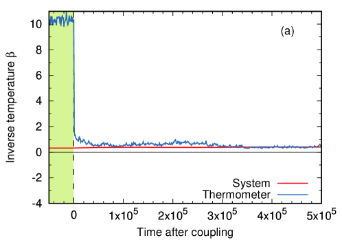
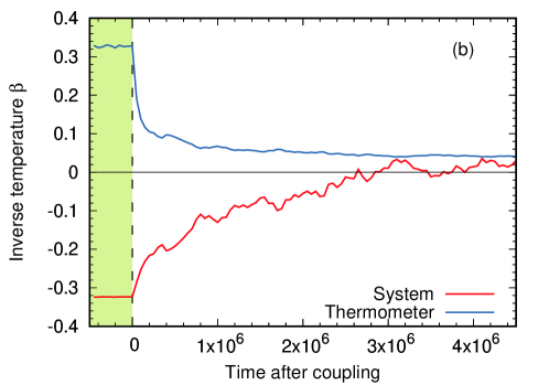
Figure 6: Inverse temperature $\beta$ as a function of time, for the sample (99) and the positive-temperature thermometer (100). In panel (a) a case in which both subsystems start at positive temperature is shown, while in panel (b) the sample is prepared in a NAT equilibrium state. The inverse temperature $\beta(t)$ of the sample is computed from a fit on the single particle momentum pdf: we consider the histogram of the measured momenta from time $t$ to time $t+\Delta t$, with $\Delta t=5\cdot 10^{4}$ in this case, and we obtain the value of $\beta$ from the slope of $\log[\rho(p)]$, as explained in Ref. cerino15 . Thermometer’s inverse temperature has been determined, as usual, by $\beta=\langle p^{2}\rangle^{-1}$. The shape of the interaction potential between the sample and the thermometer appearing in Eq. (98) is $\mathcal{V}(x)=1-\cos(x)$. Parameters: $N_{S}=100$, $N_{T}=30$, $K=\gamma=0.5$, $J=0.05$ $\varepsilon=0.1$. Figure adapted from Ref. baldovin17 .

First, let us consider a case in which the thermometer does not admit negative temperature:

$$\mathcal{H}_{T}=\sum_{i=0}^{N_{T}}\frac{p_{i}^{2}}{2}+\sum_{i=1}^{N_{T}}m\gamma^{2}\left[1-\cos(\phi_{i}-\phi_{i-1})\right]\,;$$ (100)

the kinetic energy of the thermometer is the usual quadratic one, so that NAT cannot be reached. Figure 6 shows that, if the sample is initially prepared in a positive-temperature state, the thermometer is able to reach its temperature and measure it without relevant perturbations. On the other hand, if the sample is in a NAT state for $t<0$, when the coupling is switched on its inverse temperature starts increasing, due to an energy flux from the sample to the thermometer. This process only ends when both systems reach a common, positive temperature. The amount of the exchanged energy is huge even if the size of the thermometer and its coupling with the system are small (i.e. $N_{T}/N_{S}\ll 1$, $\epsilon\ll 1$). The final state of the sample is significantly different from the initial one, so that we must conclude, as it could be expected from the beginning, that this kind of thermometer is not suitable at all to measure the temperature of systems at negative temperature.

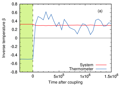
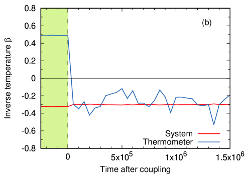
Figure 7: Inverse temperature $\beta$ as a function of time, for the system (99) and the thermometer (101), both measured by the distribution fitting procedure explained in Fig 6. In panel (a) the sample is initially prepared in a positive-temperature state, in panel (b) its initial $\beta$ is negative. The shape of the interaction potential between the sample and the thermometer appearing in Eq. (98) is $\mathcal{V}(x)=1-\cos(x)$. Parameters: $N_{S}=100$, $N_{T}=30$, $K=\gamma=0.5$, $J=0.05$ $\varepsilon=0.1$. Figure adapted from Ref. baldovin17 .

Let us now study what happens if the thermometer is properly chosen, i.e. if its Hamiltonian coordinates, as well as those of the sample to be measured, live in a bounded phase space:

$$\mathcal{H}_{T}=\sum_{i=0}^{N_{T}}(1-\cos p_{i})+\sum_{i=1}^{N_{T}}\gamma\left[1-\cos(\phi_{i}-\phi_{i-1})\right]\,.$$ (101)

Now the temperature cannot be estimated by the mean kinetic energy, so we have to adopt an appropriate methodology, e.g. use Rugh’s definition or look at the shape of the probability distribution of the single particle momentum, the generalized Maxwell-Boltzmann $\rho(p)\propto e^{-\beta[1-\cos(p)]}$, see Eq. (86). With this kind of thermometer a correct measurement of the temperature can be performed, as shown in Fig. 7.

We conclude by noticing that the details of $\mathcal{H}_{T}$ are not particularly important: the relevant aspects are the bounded nature of the phase space and the fact that $N_{T}$ is small with respect to $N_{S}$. These conditions should be sufficient, in general, to insure that the thermometer equilibrates with the sample within an acceptable time and without perturbing it significantly, allowing therefore to measure the system’s temperature by looking at accessible observables.

IV.3 Ensemble equivalence (and its violations)

The relation between ensemble equivalence and negative temperatures is far from straightforward and deserves a careful consideration. As a general remark, let us briefly consider the role of $T_{B}$ in the context of the problem of the equivalence of the ensembles. If we limit our attention to systems with short-range interactions, we can assume, following the usual arguments that can be found in textbooks, that

$$S_{B}(E,N)=Ns(e)\,,$$ (102)

i.e. the entropy is an extensive quantity (here $e=E/N$ and $s(e)$ is the entropy per particle); moreover, $s(e)$ cane be assumed to be concave, so that, performing a steepest descent analysis in the large-$N$ limit, one obtains the canonical description from the (Boltzmann) microcanonical one, e.g.:

$$T_{B}(e)s(e)=e-f(T_{B}(e)),$$ (103)

where $f(T)$ is the free energy per particle in the canonical ensemble. In such a derivation, the only relevant point is the convexity of $s(e)$, and nothing about its first derivative is asked: therefore, the equivalence of ensembles naturally holds even when $T_{B}$ assumes negative values. Since $T_{B}$ and $T_{G}$ can be different even for large $N$, it is evident that $T_{G}$ is not relevant for the determination of equivalence between statistical ensembles.

In this Section we aim at summarizing the overall scenario, while illustrating in some detail the following points:

• there are examples of simple statistical models defined on a discrete lattice exhibiting negative temperature equilibrium states without any violation of the equivalence of statistical ensembles, provided the definition of Boltzmann’s microcanonical temperature $\beta^{-1}_{B}$ (see Sec. III.1) is adopted;

• for these simple models the Gibbs’ microcanonical temperature $\beta^{-1}_{G}$ is found to be inconsistent with ensemble equivalence;

• there is evidence that in more elaborated lattice models the equivalence between equilibrium statistical ensembles may fail in the negative temperature phase, because of specific physical reasons.

IV.3.1 Simple models

Let us first discuss the classical model of the Discrete Linear Schrödinger Equation, i.e. the noninteracting version of the model discussed in Sec. II.5, defined on a 1d lattice of $N$ sites with periodic boundary conditions, whose Hamiltonian reads

$${\mathcal{H}}=-\sum_{j=1}^{N}(z_{j}\,z^{*}_{j+1}+c.c.)\,,$$ (104)

where $z_{j}$ is the complex amplitude of the wave function at site $j$. The choice of the minus sign in front of the r.h.s. of this equation is essentially irrelevant, because of the symmetry associated to the gauge transformation $z_{j}\to e^{i\pi j}\,z_{j}$, with $i$ representing the imaginary constant. This Hamiltonian model can be interpreted as a system of noninteracting particles, hopping on a lattice: it conserves not only the energy ${\mathcal{H}}$, but also the quantity $A=\sum_{j=1}^{N}|z_{j}|^{2}$. If one interprets $|z_{i}|^{2}$ as the number of particles at site $j$, the total norm $A$ is the total number of particles in the lattice. For practical reasons it is worth introducing the energy and norm densities

$$h=\frac{{\mathcal{H}}}{N}\,,\quad\quad a=\frac{{\mathcal{N}}}{N}\,.$$ (105)

The grand-canonical partition function of this simple model is defined as follows

$${\mathcal{Z}}=\int\prod_{j=1}^{N}dz_{j}e^{-\beta N(h-\mu a)}\,,$$ (106)

where $\mu$ is the chemical potential. The explicit calculation of ${\mathcal{Z}}$ can be easily performed (e.g., see buonsante16 ; buonsante17 ) by introducing the Fourier-transformed variables

$$\tilde{z}_{k}=(1/N)\sum_{j=1}^{N}e^{i\,kj}z_{j}\,,\quad\quad k=0,\dots,N-1\,,$$ (107)

and one can write

$${\mathcal{H}}=\sum_{k=0}^{N-1}\epsilon_{k}|z_{k}|^{2}\,,\quad\quad A=\sum_{k=0}^{N-1}|z_{k}|^{2}\,,$$ (108)

where

$$\epsilon_{k}=-2\cos(2\pi k/N)$$ (109)

is the energy associated to the $k$-th Fourier mode. The grand-canonical partition function turns out to have the explicit expression

$${\mathcal{Z}}=\prod_{k=0}^{N-1}\frac{\pi}{\beta(\epsilon_{k}-\mu)}\,,$$ (110)

The average norm density and the average energy density are given by the expressions buonsante16

$$a=\frac{N}{N}=\frac{1}{N}\sum_{k=0}^{N-1}\langle|\tilde{z}_{k}|^{2}\rangle=\frac{1}{N}\sum_{k=0}^{N-1}\frac{1}{\beta(\epsilon_{k}-\mu)}\,,\quad\quad h=\frac{1}{\beta N}\sum_{k=0}^{N-1}\frac{\epsilon_{k}}{\epsilon_{k}-\mu}\,.$$ (111)

In the limit of large values of $N$ one can obtain the explicit form of the inverse temperature and of the chemical potential in terms of $a$ and $h$:

$$\mu = \frac{h^{2}+4a^{2}}{2ah}$$ (112)

$$\beta = -\frac{2h}{4a^{2}-h^{2}}\,.$$ (113)

Notice that $\beta$ is positive for $-2a<h<0$, but it is negative for $0<h<2a$. On the other hand there is no thermodynamic difference between the two phases at positive and negative temperatures, because they are related by the gauge symmetry intrinsic to this model: in fact, changing the sign in front of (104) amounts to exchange these two phases, i.e. $\beta\to-\beta$.

For this simple model one can compute explicitly also the Boltzmann microcanonical entropy density

$$s_{B}(h,a)=\frac{1}{N}k_{B}\ln(\omega(h,a)\,C)\,,$$ (114)

where $\omega(h,a)$ is the density of states for given values of $h$ and $a$, in formulae

$$\omega(h,a)=\int\prod_{k=0}^{N-1}{\mathrm{d}}z_{k}\,\delta(Nh-{\mathcal{H}})\,\delta(Na-A)$$ (115)

and $C$ is a suitable constant with the physical dimensions of $h$. The complete expression of $\omega(h,a)$ is reported in buonsante16 . For our purposes it is enough to observe that for large values of $N$ this expression boils down to

$$\omega(h,a)\propto\Big{(}\frac{4a^{2}-h^{2}}{a^{2}}\Big{)}^{N}$$ (116)

By recalling the definition of the Boltzmann inverse temperature $\beta_{B}=\frac{1}{k_{B}}\frac{\partial s(h,a)}{\partial h}$ one can immediately check that $\beta_{B}$ coincides with the inverse temperature $\beta$ obtained for the grand-canonical ensemble in Eq.(113).

These easy calculations certify that, despite the thermodynamics of this simple model admits equilibrium states at negative temperature (which are just symmetric to states with positive temperature), one has ensemble equivalence between the grand-canonical ensemble and the microcanonical one, computed by the Boltzmann entropy density (114).

Conversely, if one adopts the the definition of Gibbs microcanonical entropy density

$$s_{B}(h,a)=\frac{1}{N}k_{B}\ln(\Omega(h,a)\,C^{\prime})\,,$$ (117)

where

$$\Omega(h,a)=\int_{-2a}^{h}\,{\mathrm{d}}h^{\prime}\,\omega(h^{\prime},a)\,,$$ (118)

one obtains that the Gibbs inverse temperature verifies $\beta_{G}(h,a)=\beta_{B}(h,a)$ only for $h\in[-2a,0)$ (i.e. in the region where $\beta_{B}(h,a)$ is positive), while it vanishes identically for $h\in(0,2a]$, where $\beta_{B}$ and $\beta$ coincide and are both negative (see buonsante17 ). This testifies that Gibbs’ entropy violates ensemble equivalence. Let us remark that the lower bound $-2a$ of the integral in Eq.(118) comes from observing that, for a given value $a$ of the norm density, the energy density $h$ is bounded in the interval $[-2a,2a]$.

Another simple model exhibiting analogous features is described by the Hamiltonian

$${\mathcal{H}}=-\varepsilon\,\sum_{j=1}^{N}\sigma_{j}\,,$$ (119)

already introduced in Sections II.2 and III.3.2 (see also dunkel14 ; campisi15 ; campisi16 ). This model represents a lattice of $N$ uncoupled spin variables $\sigma_{j}=\pm 1$; $\varepsilon$ is a constant depending on the gyromagnetic ratio of the spins and the applied field. It is the simplest example of the class of models discussed in the celebrated paper by Ramsey about negative temperature equilibrium states in nuclear spin systems ramsey56 . As reported in buonsante16 , the calculation of the canonical partition function is straightforward, yielding the expression

$$Z=\Big{[}2\cosh(\beta\,\varepsilon)\Big{]}^{N}=e^{-\beta\,F}\,,$$ (120)

where, again, $\beta$ is the inverse temperature in units of the Boltzmann constant $k_{B}$ and $F$ is the Helmholtz free energy. Standard thermodynamic relations allow to obtain the explicit expressions of the internal energy $E$:

$$E=-\frac{\partial}{\partial\beta}\log Z=-N\varepsilon\tanh(\beta\varepsilon)$$ (121)

and of the entropy $S$:

$$S=k_{B}\,\beta^{2}\,\frac{\partial F}{\partial\beta}=k_{B}\,N\,\Big{[}\log 2+\log(\cosh(\beta\varepsilon))-\beta\varepsilon\tanh(\beta\varepsilon)\Big{]}\,.$$ (122)

It is worth introducing the dimensionless quantity $\lambda=E/(N\varepsilon)$ ($-1<\lambda<1$) to write the expression of the inverse temperature (which is obtained by inverting Eq.(121) )

$$\beta=-{\mathrm{arctanh}}(\lambda)$$ (123)

and of the entropy

$$S=\frac{k_{B}\,N}{2}\Big{[}2\log 2-(1+\lambda)\log(1+\lambda)-(1-\lambda)\log(1-\lambda)\Big{]}$$ (124)

The first equation indicates that negative temperature equilibrium states are obtained for $0<\lambda<1$, while the second equation tells us that $S$ is a concave function of $\lambda$ and exhibits a maximum at $\lambda=0$. It is worth pointing out that $\beta$ and $S$ obtained for the canonical ensemble satisfy the same relation, that is expected to hold for the microcanonical ensemble $\beta=1/k_{B}\,\frac{\partial s}{\partial\lambda}$, with $N\,s=S$.

For this model one can compute explicitly also the Boltzmann entropy $S_{B}$, which reads (see buonsante16 )

$$S_{B}=k_{B}\log(\omega(\lambda))\,,$$ (125)

where

$$\omega(\lambda)=\frac{N!}{(\frac{1+\lambda}{2}N)!\,(\frac{1-\lambda}{2}N)!}$$ (126)

By applying the Stirling approximation of the factorial one can easily check that $S_{B}$ coincides with $S$ for large values of $N$. Conversely, the Gibbs entropy $S_{G}$ reads (see buonsante16 )

$$S_{G}=k_{B}\log(\Omega(\lambda))\,,$$ (127)

where

$$\Omega(\lambda)=\frac{N}{2}\int_{-1}^{\lambda}{\mathrm{d}}\lambda^{\prime}\,\omega(\lambda^{\prime})\,.$$ (128)

It can be easily verified that in the region of positive temperatures, $-1<\lambda<0$, one has $\beta_{G}\equiv 1/(k_{B}\,N)\,\frac{\partial S_{G}}{\partial\lambda}=\beta_{B}\approx\beta$, while in the region of negative temperatures, $0<\lambda<1$, $\beta_{G}=0$. Accordingly we are facing the same scenario previously described for the free-hopping-particle model (104).

IV.3.2 A wider scenario

The pedagogical examples discussed in the previous section point out that the equivalence of equilibrium statistical ensembles, which is expected to hold for standard short-range interacting systems at positive temperature, may be extended also to negative-temperature equilibrium states, provided the Boltzmann definition of microcanonical entropy is adopted (e.g., see (125)). Accordingly, these examples strongly challenge the very conceptual consistency of the Gibbs microcanonical entropy (e.g., see (127)), which merely reduces to an approximate formula for estimating the Boltzmann microcanonical entropy for large values of $N$ and for positive temperatures, only. On the other hand, if one would like to attribute to Gibbs’ entropy the role of the cornerstone of equilibrium thermodynamics one might argue that negative temperature equilibrium states are just an artifact, suggested by pathologically simple models, while they have no room in real physical phenomena. In such a perspective, the experimental evidence of genuine negative-temperature equilibrium states observed by Purcell and Pound purcell51 in nuclear-spin systems and, much more recently, by various researchers in superfluid Bose-Einstein condensates gauthier19 ; johnstone19 could be reinterpreted as a manifestation of long-living metastable states. As discussed in Sec. III.3, these different points of view have raised a long-standing dispute about the physical relevance of negative temperature equilibrium states, which has eventually come to the conclusion that their existence does not contradict any basic principle of thermodynamics.

In order to enforce the physical interest for these states, in what follows we want to shortly illustrate more elaborated models, where they appear also when the equivalence between equilibrium statistical ensembles is violated.

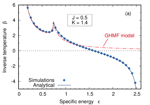
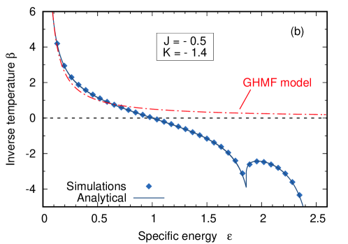
Figure 8: Dependence of $\beta$ on the specific energy in the Hamiltonian model (129), living in bounded phase space, and in the corresponding GHMF model introduced in Ref. debuyl05 . Two choices of the parameters are considered: $J=0.5$, $K=1,4$ (panel (a)) and $J=-0.5$, $K=-1,4$ (panel (b)). For both cases, numerical simulations in the microcanonical ensemble (light blue diamonds) are compared with the analytical equilibrium prediction (blue solid line), obtained with large-deviations techniques miceli19 . The values of $\beta$ are obtained from the analysis of averages of suitable observables, depending on the single-particle momentum distribution. Red dash-dotted lines represent the equilibrium behaviour of the GHMF model with the same parameters: the two models show similar features at low energy, but they differ in the high-energy limit. Size of the system $N=10^{3}$. Figure adapted from Ref. miceli19 .

The first example is a model of a 1d lattice of rotators, whose Hamiltonian reads miceli19

$${\mathcal{H}}=-\sum_{j=1}^{N}(1-\cos(p_{j}))-Nv(m)\,,$$ (129)

where

$$v(m)=\frac{J}{2}m^{2}+\frac{K}{4}m^{4}+C\,,$$ (130)

with

$$m=|{\bf m}|\,,\quad{\bf m}=\frac{1}{N}\Big{(}\sum_{j=1}^{N}\cos q_{j},\sum_{j=1}^{N}\cos q_{j}\Big{)}\,.$$ (131)

The canonically conjugated angular variables $q_{j}$ and $p_{j}$ are constrained to the interval $(-\pi,\pi]$; the long-range interaction among rotators is due to the nonlinear mean-field potential $v(m)$, which depends on the modulus of the magnetization vector ${\bf m}$. This is a suitably modified version of the Generalized Hamiltonian Mean-Field (GHMF) model debuyl05 , which exhibits a standard quadratic kinetic term of the form $\sum_{j=1}^{N}p^{2}_{j}$ (here each $p_{j}$ is a true unbounded action variable) replacing the sum on the r.h.s. of Eq.(129). The GHMF model has been widely investigated as a paradigmatic example of a long-range interacting system which exhibits inequivalence between statistical ensembles in correspondence of a magnetic transition debuyl05 . As discussed in miceli19 , the modified kinetic term in (129) allows one to obtain negative-temperature equilibrium states, because of the boundedness of the phase-space yielding an energy range with decreasing entropy. It is worth recalling again here that, as discussed in other sections of this review (see I.3, III.3), this peculiar feature of the phase-space is a basic ingredient for observing negative-temperature equilibrium states in similar models. The behaviour of the caloric curve of model (129), i.e. $\beta\,{\mathrm{v}s}.\,\epsilon={\mathcal{H}}/N$, has been obtained by large-deviation techniques and further checked by numerical simulations of the Hamiltonian dynamics (see miceli19 : as discussed in this reference the non-quadratic form of the kinetic term demands the use of a suitable relation for obtaining the numerical estimate of $\beta$). For positive values of the parameters $J$ and $K$ the magnetic transition is found to occur at positive temperature (see Fig. 8(a)), while the equivalence between equilibrium statistical ensembles if found to extend out of the transition region, including the negative temperature phase which is observed for large enough values of $\epsilon$. For negative values of $J$ and $K$ the magnetic transition moves to the region of negative temperatures and also in this case inequivalence between equilibrium statistical ensembles is observed in the transition region (see Fig. 8(b)). In particular, this feature has been tested numerically by comparing the probability distributions of the angular variable $q_{j}$ obtained by the dynamics of an isolated chain (microcanonical setup) and by the stochastic Langevin-like dynamics, simulating the interaction with a thermal reservoir: in the transition region where the microcanonical specific heat is predicted to be negative these two probability distributions do not match each other (see Fig. 9). In summary, this model provides us with additional relevant information about the relation between negative temperature equilibrium states and equivalence between statistical ensembles:

• apart the region of the magnetic transition we are facing the same scenario provided by the simple models discussed in the previous section, which rules out a consistent description of the thermodynamics of this model making use of the Gibbs’ entropy;

• inequivalence between statistical ensembles may occur also at negative temperature around a phase transition, but this is due to the same mechanism occurring at positive temperature, i.e. the metastability of microcanonical states, yielding negative specific heat.

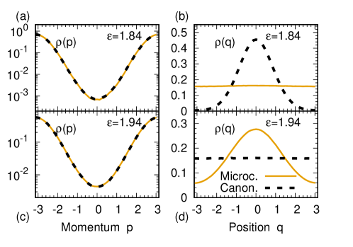
Figure 9: Inequivalence between canonical and microcanonical ensemble for model (129) with $J=-0.5$, $K=-1.4$. The microcanonical equilibrium state described by a given specific energy $\epsilon=\mathcal{H}/N$ is compared to the corresponding canonical state at the same inverse temperature. Two cases are shown in which, even if the pdf of the single-particle momentum is identical in the two ensembles (panel (a): $\epsilon=1.84$; panel (c):$\epsilon=1.94$), the positions of the particles behave in a completely different way (panel (b): $\epsilon=1.84$; panel (d): $\epsilon=1.94$). The canonical ensemble has been reproduced by mean of a Langevin-like stochastic bath, see Ref. miceli19 for details, and the general discussion in Section V.1 of the present review. Figure adapted from Ref. miceli19 .

The last example we want to discuss here is the Hamiltonian lattice model yielding the Discrete Nonlinear Schrödinger Equation:

$${\mathcal{H}}=\sum_{j=1}^{N}(z_{j}\,z^{*}_{j+1}+c.c.)+\sum_{j=1}^{N}|z_{j}|^{4}\,.$$ (132)

Without prejudice of generality, here the Hamiltonian (37) has been turned to the simplified form where $\Lambda=2$. It can be viewed as the nonlinear version of model (104) with a quartic nonlinearity. This model has been extensively studied, because of its phenomenological interest for many physical applications, e.g. Bose-Einstein condensates in optical lattices TS ; franzosi11 and light propagating in arrays of optical waveguides ESMBA . As well as (104), this nonlinear model conserves the total energy and the total number of particles in the lattice, $A=\sum_{i=1}^{N}|z_{i}|^{2}$. The problem of the equivalence between equilibrium statistical ensembles and negative temperature states in this model is discussed in detail in Section VI. Here we just summarize the specific situation emerging in this problem, which further enriches the overall scenario. The thermodynamics of model (132) is summarized by the phase diagram in Fig. 3. No physical states are accessible below the $(\beta=+\infty)$-line, $h=a^{2}-2a$, $h$ and $a$ being respectively the densities $H/N$ and $A/N$. Between this line and the $(\beta=0)$-line, $h=2a^{2}$, one has positive temperature states and equivalence between statistical ensembles. At variance with the previous model, the phase-space is unbounded. This notwithstanding, for energies above the $(\beta=0)$-line the microcanonical Boltzmann entropy is found to decrease with $h$. In particular, it has been shown GILM1 that large-deviation techniques allow one to obtain an analytic estimate of $S_{B}$, which indicates that for large values of $N$, $\beta_{B}$ is actually negative. On the other hand, the same estimate rules out the possibility of the equivalence of the microcanonical ensemble with the grand-canonical one in the phase where $\beta_{B}<0$, because of the very analytic structure of $S_{B}$, which forbids to express the grand-canonical partition function ${\mathcal{Z}}$ as a Fenchel-Legendre transform of $S_{B}$ (for details see GILM1 ; GILM2 ). What makes the difference between this model and all the previously described ones is the physical mechanism ruling the phase at negative temperature, i.e. the region above the line $h=2a^{2}$. Actually, numerical simulations of the Hamiltonian dynamics (e.g. see franzosi11 ; ICOPP ) indicate the formation of localized excitations in the form of breathers, which may live over extremely long time spans (the larger their amplitude the less they interact with the radiation background) and then may be born again by large fluctuations at some lattice site. Thermodynamics predicts that, apart a small region just above the line $h=2a^{2}$, which vanishes in the thermodynamic limit, all breathers should coalesce into a single giant breather collecting a macroscopic portion of the total energy GILM1 ; GILM2 . In fact, at variance with solitons, breathers interact between themselves, like in a fish-species dynamics, where the larger typically eats the smaller. On the other hand, this coalescence mechanism seems to never come to the expected end in the dynamics of an isolated DNLS chain, even for moderate system size $N$: the transient to equilibrium is strongly inhibited by localization. Conversely, stochastic numerical simulations conserving both ${\mathcal{H}}$ and $A$ yield the expected equilibrium configuration through a coarsening process ruled by predictable scaling properties Iubini14 ; Iubini17 . As a concluding remark about microcanonical thermodynamics, it is worth mentioning that in the thermodynamic limit negative temperature states boil down to infinite-temperature ones GILM1 .

We want to conclude this section by pointing out that one can perform also canonical simulation in the $\beta<0$ region of the DNLS model by exploiting inverse Monte Carlo protocols or Langevin-like heat reservoirs acting on a DNLS chain. As one can easily guess, the localization mechanism of energy into breather states allows one to pump from thermodynamic fluctuations induced by the reservoirs an arbitrary amount on energy and norm into the system, which eventually “explodes”, thus providing evidence that, as already reported in the seminal book by D. Ruelle Ruelle , physical condensation mechanisms may play a major role in the nonequivalence of statistical equilibrium ensembles. This point will be further discussed in Section VII.2.

V Fluctuation-dissipation and response theory

In the last Section we discussed in which sense the notion of equilibrium at NAT is physically meaningful, and to what extent it is consistent with statistical mechanics. In what follows we focus instead on fluctuation-dissipation relation (FDR) and response theory: this can be seen as a first step toward a generalization of out-of-equilibrium statistical mechanics to cases with NAT, a topic which will be also faced in Section VII. First we discuss a stochastic differential equation (a “generalized” Langevin equation) to describe the motion of particles interacting with NAT heat baths. Such thermal reservoirs may be composed, for instance, by many “lighter” particles with smaller inertia, or by a lattice of Ising spins with their own stochastic dynamics; the overall result does not depend significantly on these details. The validity of FDR, linking spontaneous correlations to the linear response induced by an external perturbation, is then investigated when NAT is present.

V.1 Langevin equation with $\beta<0$

One of the pillars of out-of-equilibrium statistical mechanics is the possibility to write a Langevin equation, i.e. an effective description for the slow motion of a “heavy” particle (mass $M$) interacting with many “light”, fast degrees of freedom (mass $m\ll M$). Such a problem was originally faced with a phenomenological approach by Paul Langevin in his seminal paper on the Brownian motion of a colloidal particle in a fluid langevin . Langevin’s analysis grounds on the assumption that the heavy particle’s behaviour is determined by two competing elements, whose combined effect allows for the thermal equilibrium at temperature $T$: (i) the viscous force given by Stokes law; (ii) the presence of random thermal fluctuations. The resulting differential stochastic equation reads

$$\frac{dP}{dt}=-\frac{\gamma}{M}P(t)+\sqrt{2\gamma k_{B}T}\xi(t)\,,$$ (133)

where $P(t)$ is the momentum of the heavy particle, $T$ is the temperature of the system and $\xi$ is a Gaussian white noise: $\langle\xi(t)\rangle=0$, $\langle\xi(t)\xi(t^{\prime})\rangle=\delta(t-t^{\prime})$.

Actually, only in few cases it is possible to obtain the Langevin equation (133) analytically, determining the friction parameter $\gamma$ from first principles. Important examples are the motion of a heavy intruder in a chain of harmonic oscillators rubin60 ; turner60 ; takeno-hori62 ; ford-kac-mazur65 ; zwanzig73 and that of a tracer in a gas of elastic hard disks (or beads, in 3-dimensional space) with very low density smoluchowski06 ; dorfman70 ; dorfman09 . Usually Eq. (133) is instead assumed to be a valid model for the considered phenomenon, and its effectiveness is checked a posteriori.

Langevin-like equations hold also in cases with NAT. For instance, it has been shown that it is possible to determine drift and a diffusion coefficients accounting for the effective motion of a single vortex in two-dimensional hydrodynamics chavanis98 ; chavanis07 ; yatsuyanagi15explicit ; as discussed in Section II.1, NAT can be observed, as a consequence of the bounded nature of the Hamiltonian coordinates space, as soon as the system is constrained in a finite domain. The drift term of this Langevin equation explicitly depends on $\beta$, in such a way that states with opposite temperature correspond to qualitatively different dynamics: if $\beta>0$ the vortex is repelled from the center of the domain, whereas if $\beta<0$ it is attracted chavanis98 .

In what follows we discuss a generalized Langevin equation, valid for mechanical models of the form (85) already encountered in the previous Section. In this kind of systems, at variance with the case of vortices, the Hamiltonian includes generalized kinetic terms $\mathcal{K}(p)$ explicitly depending on the single particle momentum: in this sense the resulting stochastic differential equation is a direct generalization of Eq. (133), which is recovered as a particular case. We will consider systems composed by a large number $N$ of fast, microscopic degrees of freedom (the “bath”) and a slow, mesoscopic one (the “tracer”). The physical meaning of this scale separation and its relation to a generalized notion of inertia for Hamiltonians of the form (85) will be outlined in the following subsection. By now we shall just assume, as a work hypothesis, that the typical times of the tracer dynamics result much longer than those of the bath.

The Hamiltonian of the whole systems reads

$$\mathcal{H}(P,\{p_{n}\},Q,\{q_{n}\})=\mathcal{K}(P)+\sum_{n=1}^{N}{\mathcal{K}^{\prime}}(p_{n})+\mathcal{U}(Q)+\mathcal{V}(Q,\{q_{n}\})$$ (134)

where $(P,Q)$ are the canonical coordinates of the mesoscopic tracer, $(p_{n},q_{n})$ those of the $n$-th particle of the bath. Of course in the equations of motion for the tracer there appear terms depending on the coordinates of the fast particles constituting the bath:

$${d\over dt}Q=\partial_{P}K(P)\,\,\,,\,\,\,{d\over dt}P=-\partial_{Q}U(Q)-\partial_{Q}V(Q,\{q_{n}\})\,.$$ (135)

Within the mentioned time-scale separation hypothesis it is reasonable to write down an effective stochastic equation for the tracer:

$${d\over dt}Q =\partial_{P}\mathcal{K}(P)$$ (136)

$${d\over dt}P =-\partial_{Q}\mathcal{U}(Q)+\Gamma(P)+\sqrt{2D}\xi(t)\,,$$

where the interactions with the microscopic degrees of freedom of the bath are mimicked by a “friction” term $\Gamma(P)$ and a noisy force depending on a diffusivity $D$. If this effective description actually holds, we are only left with the problem of determining the shape of $\Gamma(P)$ and the value of $D$.

In this respect, a simple phenomenological argument can be outlined as follows. Let us define the steady probability density $f(Q,P)$ for the coordinates of the tracer, and the currents

$$J_{Q}(Q,P)=f(Q,P)\partial_{P}\mathcal{K}(P)$$ (137)

$$J_{P}(Q,P)=-f(Q,P)\partial_{Q}\mathcal{U}(Q,P)+\Gamma(P)f(Q,P)-D\partial_{P}f(Q,P)\,.$$ (138)

The associated Fokker-Planck equation reads:

$$\partial_{Q}J_{Q}(Q,P)+\partial_{P}J_{P}(Q,P)=0\,.$$ (139)

Assuming detailed balance (i.e. thermal equilibrium), the irreversible part of current (138) must vanish:

$$\Gamma(P)f(Q,P)-D\partial_{P}f(Q,P)=0\,;$$ (140)

as a consequence, by exploiting the factorization

$$f(Q,P)=f_{Q}(Q)f_{P}(P)\propto e^{-\beta[\mathcal{K}(P)+\mathcal{U}(Q)]}$$ (141)

one finds

$$\Gamma(P)=-D\beta\partial_{P}\mathcal{K}(P)\,.$$ (142)

The general version of the Langevin equation for the tracer is then

$$\frac{d}{dt}P=-D\beta\partial_{P}\mathcal{K}(P)+\sqrt{2D}\xi(t)\,,$$ (143)

where $D$ is a diffusivity term, which fixes the time scale of the dynamics. No assumption has been made about the sign of $\beta$, which can assume, in principle, negative values. This has no influence on the diffusivity, but changes the sign of the drift term. In the usual case $\mathcal{K}(P)=P^{2}/2M$ we recover the linear form for the drift term, with a viscous coefficient satisfying the familiar Einstein relation

$$\gamma=D\beta\,.$$ (144)

The validity of Eq. (143) can be numerically tested in the following way. First, one runs molecular dynamics simulations of a Hamiltonian system of the form (134), including both tracer and thermal reservoir, according to a deterministic evolution rule. The particles composing the thermal bath should have very fast decorrelation times, so to avoid memory effects; in this way the evolution of $P$ may be expected to be Markovian. The tracer’s coordinates are measured with high sampling frequency, as a function of time, disregarding the dynamics of the fast particles; the resulting trajectory $(P(t),Q(t))$ is then analyzed, a posteriori, with usual Langevin equation reconstruction techniques peinke11 ; peinke19 , in order to find the stochastic differential equation which reproduces the dynamics to the best extent. In other words, one has to find, from numerical data, the drift $F(P)$ and diffusivity $D$ such that

$$\frac{dP}{dt}=F(P)+\sqrt{2D}\xi(t)$$ (145)

is a good model for the coarse-grained dynamics of the slow particle. This task can be achieved, in principle, by exploiting the very definition of $F$ and $D$ as limits of the conditioned moments gardiner85

$$F(P)= \lim_{\Delta t\to 0}\,\frac{\langle\Delta P|P(t_{0})=P\rangle}{\Delta t}$$ (146)

$$D(P)= \lim_{\Delta t\to 0}\,\frac{\langle\Delta P^{2}|P(t_{0})=P\rangle}{2\Delta t}\,.$$

When dealing with numerical simulations the notion of $\Delta\to 0$ limit has to be handled with some care, since the time scale of $\Delta$ at which such limit is evaluated has to be small with respect to typical time-scales of the dynamics, but still much larger than the time-step of the numerical integration.

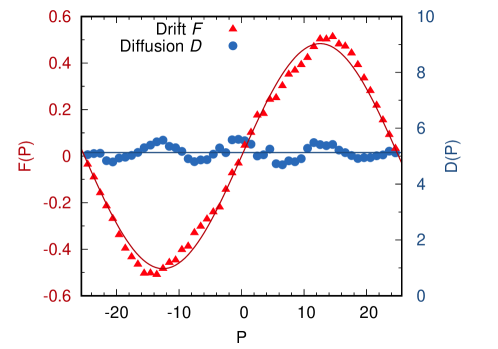
Figure 10: Drift and diffusivity reconstruction for the Langevin equation of $P$ for a model with kinetic energy (147), in a case with negative temperature. Based on numerical simulations of the whole system, the observables (146) are plotted (points) and compared with the functional forms (solid lines) which can be guessed from the argument in the main text, see Eq. (143). Here $\beta=-0.1$; the considered particle, with generalized “mass” $M=8$ (see also Section V.2), interacts with a bath composed by $N=600$ particles with mass $m=1$. Figure adapted from Ref. baldovin18 .

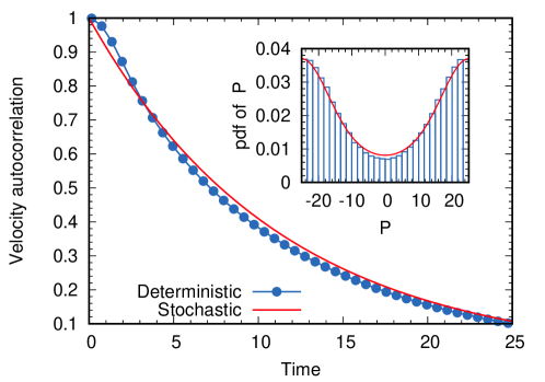
Figure 11: In the same conditions of Fig. 10, velocity autocorrelation function (main plot) and momentum distribution (inset) for the slow particle. Points and the histogram refer to the values measured in the original, complete dynamics; red solid lines show the predictions of the coarse-grained dynamics obtained as described in the main text. Figure adapted from Ref. baldovin18 .

The proposed check has been done in Ref. baldovin18 for the particular case

$$\mathcal{K}(P)=1-\cos(P)\,.$$ (147)

Leaving apart, for a moment, the problem of modeling the thermal bath (we shall discuss it in the following subsection), we can already anticipate the results of this analysis. In Fig. 10 the reconstructed functional forms of drift and diffusivity are shown to be consistent with Eq. (143), in a case at negative temperature. Let us notice that the sign of $\beta$ influences the qualitative behaviour of the drift term, which in this case is positive when $P>0$ and negative when $P<0$ (in a positive-temperature scenario the behaviour would have been opposite). Figure 11 shows instead the good agreement between the original, complete dynamics and the Langevin equation (143), both for static and dynamic observables (namely, equilibrium p.d.f. and velocity autocorrelation function).

V.2 Thermal baths at negative temperature

The mesoscopic motion of a particle with generalized kinetic energy can be described by a Langevin equation of the form (143) with $\beta<0$ when the tracer is coupled to a thermal bath at NAT. Such a reservoir should be composed by a large set of microscopic degrees of freedom living in bounded phase spaces, isolated from ordinary-matter environment, but coupled with the mesoscopic particle under study. To avoid memory effects in the noise term, the dynamics of the microscopic particles belonging to the bath should be much faster than that of the tracer. It is natural to wonder whether this thermal bath is physically meaningful, i.e. if it is possible to think of a high-dimensional dynamics whose effect is actually described by Eq. (143) also when $\beta<0$.

A minimal model can be implemented, for Hamiltonian systems of the form (134), by a direct generalization of the notion of inertial mass to systems with generic kinetic terms. We ask a very natural physical condition to be satisfied, i.e. that the momentum and the kinetic energy of particles moving with the same velocity are proportional to the masses. This extensivity criterion is quite reasonable: indeed, if $n$ particles with mass $m$ and momentum $p$ are stucked together (and, therefore, they move with the same velocity), we expect their behaviour to be indistinguishable from that of a single particle with mass $nm$, momentum $np$ and total kinetic energy equal to $n$ times the one of the single particle. In formulae

$$\mathcal{K}(np,nm)=n\mathcal{K}(p,m)\,.$$ (148)

It is easy to check that the above condition is verified by kinetic terms of the form

$$\mathcal{K}(p,m)=mc^{2}k(p/cm)\,,$$ (149)

where $k(x)$ is an even function and $c$ is a constant with the physical dimensions of a velocity. The function $k$ needs to be even in order to preserve spatial isotropy. For instance, let us remark that choosing $k(x)=x^{2}/2$ leads to the usual kinetic energy of classical mechanics (and no dependence on $c$ appears), while $k(x)=\sqrt{1+x^{2}}$ gives the relativistic one ($c$ being the light velocity in that context).

With this picture in mind, we can simulate a thermal bath for the tracer with kinetic energy (147) by considering a large set of microscopic particles of the same nature, but with smaller masses:

$$\mathcal{H}=M[1-\cos(P/M)]+\sum_{n=1}^{N}m[1-\cos(p_{n}/m)]+\mathcal{U}(Q)+\mathcal{V}(Q,\{q_{n}\})\,,$$ (150)

where $m\ll M$ and we have set $c=1$. To obtain the results shown in Fig.s (10) and  (11) one can choose $\mathcal{V}(Q,\{q_{n}\})$ in such a way that the particles of the bath exchange heat between themselves and some of them are also coupled to the tracer: this should prevent the presence of memory effects in the noise term, and insure as well thermal equilibrium among the particles of the bath baldovin18 .

Of course the above discussed Hamiltonian approach is not the only possible choice to model a bath at NAT. In many cases a thermal bath can be constituted by a lattice of Ising spins interacting with the tracer bonilla10 ; bonilla15 ; ruiz-garcia17 ; since Ising spins can be also found, in principle, in states with $\beta<0$ (see Section II.2), they are a promising candidate.

In Ref. baldovin19 the compound physical system

$$\mathcal{H}(P,Q,\boldsymbol{\sigma})=\mathcal{K}(P)+\mathcal{U}(Q)-\mu\lambda(Q)\sum_{n=1}^{N}\sigma_{n}$$ (151)

has been investigated, where the tracer $(P,Q)$ interacts with $N$ Ising spins $\{\sigma_{n}=\pm 1\}$. Here $\lambda(Q)$ is a function of the tracer position and $\mu$ is a constant, scaling as $N^{-1/2}$. The spin lattice follows a stochastic Glauber dynamics glauber63 , so that each spin “flips” (i.e., changes its sign) with a rate $\omega$ depending both on $\beta$ and on the external field:

$$\omega(\boldsymbol{\sigma}\to\boldsymbol{\sigma}^{\prime}_{n}|Q)=\frac{\alpha}{2}\left(1+\sigma_{n}\tanh[\beta\lambda(Q)]\right)\,,$$ (152)

where $\boldsymbol{\sigma}^{\prime}_{n}$ is the spins configuration which is obtained from $\boldsymbol{\sigma}$ by switching only the $n$-th spin, and $\alpha$ is a typical frequency of the bath. With the above stochastic evolution, the stationary pdf of the $n$-th spin, at fixed $Q$, is given by the equilibrium distribution

$$\mathcal{P}^{eq}(\sigma_{n}|Q)=\frac{e^{\sigma_{n}\beta\mu\lambda(Q)}}{2\cosh[\beta\mu\lambda(Q)]}\,,$$ (153)

and detailed balance is satisfied.

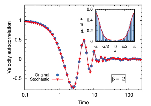
Figure 12: For model (151), velocity autocorrelation function (main plot) and momentum distribution (inset) of the oscillator. Blue circles and the histogram refer to the original dynamics, red squares and solid line to the coarse-grained stochastic dynamics deduced by mean of the Chapman-Enskog expansion. Here $\beta=-2$. Parameters: $N=10^{4}$, $\alpha=10$, $\mu=10^{-2}$. Figure adapted from Ref. baldovin19 .

The complete dynamics of the system is given by a Liouville-Master equation which evolves both the continuous pdf of the tracer and the discrete distribution of the spins. If the motion of the latter is fast enough (i.e., $\alpha\gg 1$), a Chapman-Enskog expansion can be performed, with parameter $\varepsilon=\alpha^{-1}$, in order to find an approximate equation for the time-dependent marginalized pdf of the tracer, $f(Q,P,t)$: this amounts to expanding both the total pdf

$$\mathcal{P}(P,Q,\boldsymbol{\sigma},t)=f(P,Q,t)\mathcal{P}^{eq}(\boldsymbol{\sigma}|Q)+\sum_{l=1}^{\infty}\varepsilon^{l}\mathcal{P}^{(l)}(P,Q,\boldsymbol{\sigma},t)$$ (154)

and the time derivative of $f(Q,P,t)$,

$$\partial_{t}f(Q,P,t)=\sum_{l=0}^{\infty}\varepsilon^{l}F^{(l)}(P,Q,t)\,.$$ (155)

The resulting equations can be solved order by order, leading to an approximate form very similar to those obtained with the “mechanical” bath. In particular, Eq. (143) is recovered, with the only differences that a “renormalization” of the potential occurs in this case, due to the interaction with the spins, and that the diffusivity $D$ depends on $Q$ in this case baldovin19 . Fig. 12 shows that the coarse-grained dynamics obtained with the Chapman-Enskog expansion is characterized by a behaviour quite similar to that of the original evolution: the stationary pdfs are very similar, both at positive and negative temperature, and also dynamical observables as correlation functions show a good agreement.

It is important to stress that the validity of a coarse-grained stochastic description for the dynamics of particles at negative temperature has an immediate consequence, very useful from a computational point of view, i.e. the possibility to simulate the effect of a thermal bath at negative temperature by mean of standard methods of numerical stochastic integration. An application is discussed, e.g., in Section VII.1.3. However this is not the only way to implement numerically a thermal bath at negative temperature.

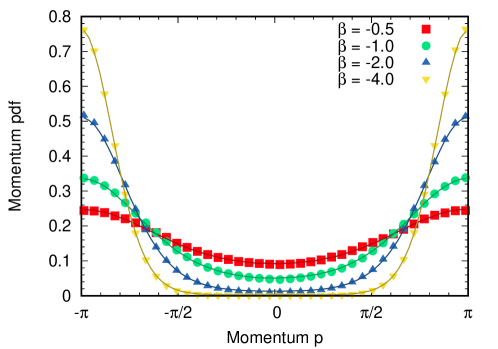
Figure 13: Comparison between Langevin stochastic bath and Monte Carlo algorithm. Model (85) with kinetic energy (87) and potential (88) is considered. Points represent histograms of the single-particle momentum distribution for Monte Carlo simulations at the (negative) inverse temperatures reported in the key. Solid lines show the results of corresponding simulations in which the extremal points of the chain are coupled to Langevin stochastic baths, as discussed in the main text. Parameters: $\delta=0.1$ for Monte Carlo, $D=0.5$ and time-step $\Delta t=0.3$ for simulations with Langevin baths. Here $N=100$.

In Ref. iubini12 ; iubini17entropy a Monte Carlo algorithm is introduced to study the equilibrium dynamics of the Discrete Nonlinear Schrödinger equation; such numerical scheme aims at reproducing the statistical properties of an equilibrium state at a given inverse temperature $\beta$; in principle, $\beta$ can be either positive or negative. As in the usual Monte Carlo, at each step a small random perturbation of the considered system (a “move”) is proposed; the move is extracted according to some fixed rule, whose optimization is usually a non-trivial task, clearly depending on the details of the considered system. The energy variation $\Delta E$ corresponding to the proposed move is then computed; the criterion to accept or reject the move is basically a generalization of the Metropolis algorithm:

• if the desired temperature is positive, the move is always accepted when $\Delta E<0$, and accepted with a probability $e^{-\beta\Delta E}$ when $\Delta E>0$;

• if, instead, the desired temperature is negative, the move is always accepted when $\Delta E>0$, and accepted with a probability $e^{-\beta\Delta E}$ when $\Delta E<0$.

The above procedure insures that the detailed balance condition between the transition rate of a move and that of its reverse is always satisfied; indeed, it is given by construction by $e^{-\beta\Delta E}$, i.e. by the ratio between the stationary probabilities of the corresponding initial states in the canonical ensemble. The possibility of negative temperature does not affect this general principle: at a practical level, it only implies that one has to pay attention to the sign of $\beta$ and apply the above rule accordingly.

In Fig. 13 the single particle momentum pdfs which can be obtained with the above discussed Monte Carlo method are shown for the already mentioned Hamiltonian chain (85) with kinetic energy (87) and potential (88). At each step one particle is randomly chosen, and the proposed move is a shift of its position and its momentum by a quantity randomly extracted from a Gaussian distribution with zero mean and variance $\delta^{2}$. A nice agreement is found with the outcomes of quasi-symplectic simulations, in which the extremal particles of the chain are coupled to Langevin-like baths reproducing Eq. (143).

V.3 Response theory

As mentioned before, FDR allows to predict the response of a system to (small) time-dependent external fields, by just analyzing time correlations in absence of perturbations.

The best known formulation of FDR is due to Kubo kubo66 , and it holds for systems at equilibrium subjected to the action of a small, time-dependent field $h(t)$. Let us denote by $\mathcal{H}_{0}({\bf x})$ the “unperturbed” Hamiltonian, ${\bf x}$ being the vector of canonical coordinates. If at time $t=0$ we turn on the external field, a small perturbation

$$\mathcal{H}_{0}({\bf x})\to\mathcal{H}_{0}({\bf x})-h(t)\mathcal{M}({\bf x})\,,$$ (156)

is induced on the system. The linear dependence on the perturbation is a mere consequence of the assumption that $h(t)$ is small, so that higher-order terms can be neglected. Response theory insures then that the quantity

$$\delta\mathcal{A}(t)=\overline{\mathcal{A}({\bf x}(t))-\mathcal{A}({\bf x}(0))}\,,$$

where $\mathcal{A}({\bf x})$ is a mechanical observable and the average $\overline{\,\cdot\,}$ is computed by repeating the experiment many times, can be expressed as kubo66

$$\delta\mathcal{A}(t)=\beta\int_{0}^{t}dt^{\prime}\left\langle\mathcal{A}({\bf x}(t-t^{\prime}))\dot{\mathcal{M}}({\bf x}(0))\right\rangle h(t^{\prime})\,,$$ (157)

where average $\langle\cdot\rangle$ is computed instead on the unperturbed system. In the above formula the inverse temperature $\beta$ appears, and no assumption on its sign is made in the derivation of Eq. (157).

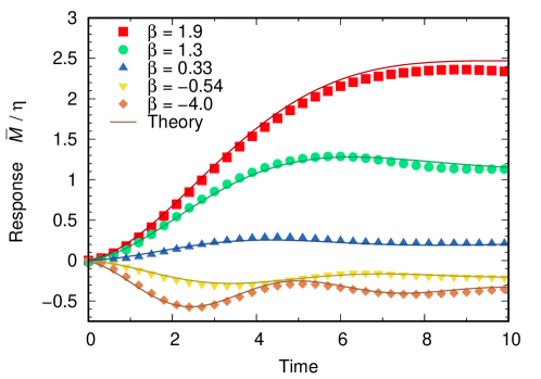
Figure 14: Check of Kubo formula in a system with NAT. For various choices of inverse temperature, both positive and negative, the measured value of the time-dependent magnetization $M$ of model (158) after the sudden switch of an external field of intensity $\eta$ is shown. Here $N=128$, $\eta=0.02$, average over $10^{4}$ realizations.

To check the validity of Kubo formula also in systems with negative temperature, we can rely again on the simple Hamiltonian model in bounded phase space discussed in Section IV.1, introducing, this time, an explicit dependence on an external field. The Hamiltonian reads

$$\mathcal{H}(\mathbf{q},\mathbf{p},t)=\mathcal{H}_{0}(\mathbf{q},\mathbf{p})-h(t)\mathcal{M}(\mathbf{q})\,,$$ (158)

where

$$\mathcal{H}_{0}(\mathbf{q},\mathbf{p})=\sum_{i=1}^{N}[1-\cos(p_{i})]+\frac{1}{2}\sum_{i=1}^{N+1}[1-\cos(q_{i}-q_{i-1})]\quad\quad q_{0}\equiv q_{N+1}\equiv 0\,$$ (159)

is the unperturbed part and

$$\mathcal{M}(\mathbf{q})=\sum_{i=1}^{N}\sin(q_{i})\,$$ (160)

can be seen as the “magnetization” associated to the external field $h(t)$.

In Fig. (14) we show the results of numerical simulations on system (158), where the external field is switched on to a value of $\eta$ at time 0, i.e.

$$h(t)=\eta\,\Theta(t)\,,$$ (161)

$\Theta(t)$ being the Heavyside step-function; magnetization $\mathcal{M}$ is then measured as a function of time. The experiment is repeated for several values of the inverse temperature $\beta$, both positive and negative, and a nice agreement is found with the Kubo formula (157), which in this case simply reads

$$\overline{\mathcal{M}(t)}=\beta\eta\int_{0}^{t}dt^{\prime}\,\langle\dot{\mathcal{M}}(0)\mathcal{M}(t^{\prime})\rangle\,.$$ (162)

Since FDR theory was initially developed within the context of equilibrium statistical mechanics of Hamiltonian systems, there has been some confusion over the years about its range of applicability. As a matter of fact, a generalized version of FDR can be shown to hold also in out-of-equilibrium conditions (i.e. in absence of detailed balance) and even for non deterministic dynamics, provided that (i) the dynamics is mixing and (ii) the system reaches an absolutely continuous and differentiable invariant probability distribution marconi08 .

The key idea is to consider the behaviour of the state ${\bf x}$ of the system when, at time $t=0$, a non-random perturbation is applied, such that

$${\bf x}(0)\to{\bf x}(0)+\delta{\bf x}_{0}\,.$$ (163)

It is easy to understand that this instantaneous “kick” modifies the initial (stationary) density $\rho({\bf x})$ of the system into a new $\rho^{\prime}({\bf x})$, related to the invariant distribution by

$$\rho^{\prime}({\bf x})=\rho({\bf x}-\delta{\bf x}_{0})\,.$$ (164)

For an infinitesimal perturbation $\delta{\bf x}_{0}=(\delta x_{1}(0)\cdots\delta x_{N}(0))$, if $\rho({\bf x})$ is non-vanishing and differentiable, it can be shown that perturbation (164) leads to (see Ref. marconi08 for the details of the derivation):

$$\overline{\delta x_{i}}\,(t)=-\sum_{j}\Biggl{\langle}x_{i}(t)\left.\frac{\partial\ln\rho({\bf x})}{\partial x_{j}}\right|_{t=0}\delta x_{j}(0)\Biggr{\rangle}\,,$$ (165)

where the meaning of the two averages is the same as before. If the protocol of the experiment is fixed and $\delta{\bf x}_{0}$ is the same for each trial, Eq. (165) can be simplified into

$$\overline{\delta x_{i}}\,(t)=\sum_{j}R_{i,j}(t)\delta x_{j}(0),$$ (166)

where we have introduced the linear response matrix

$$R_{i,j}(t)=-\Biggl{\langle}x_{i}(t)\left.\frac{\partial\ln\rho({\bf x})}{\partial x_{j}}\right|_{t=0}\Biggr{\rangle}\,.$$ (167)

The computation can be easily repeated for a generic observable $\mathcal{A}({\bf x})$, yielding

$$\overline{\delta\mathcal{A}(t)}=-\sum_{j}\left\langle\mathcal{A}({\bf x}(t))\left.\frac{\partial\ln\rho({\bf x})}{\partial x_{j}}\right|_{t=0}\delta x_{j}(0)\right\rangle\,.$$ (168)

Let us also notice that considering an impulsive perturbation is not a limitation. Indeed, in the linear regime, from the (differential) linear response one can understand the effect of a generic perturbation

$$\mathbf{F}(\mathbf{x})\to\mathbf{F}(\mathbf{x})+\delta\mathbf{F}(t)$$ (169)

of the dynamic evolution

$$\mathbf{F}(\mathbf{x})=\frac{d\mathbf{x}}{dt}\,;$$

it is enough to notice that

$$\overline{\delta x_{i}(t)}=\sum_{j}\int_{0}^{t}R_{ij}(t-t^{\prime})\delta F_{j}(t^{\prime})\,dt^{\prime}\,.$$ (170)

From Eq. (170) it is easy to recover, for Hamiltonian systems, the already mentioned Kubo formula (157).

In this general framework, it is quite clear that the presence of $\beta$ in the FRD for systems at equilibrium is related to the fact that the stationary distribution $\rho(\mathbf{x})$ explicitly depends on the inverse temperature. This is also valid, of course, for systems whose equilibrium distribution is correctly described by a negative value of $\beta$.

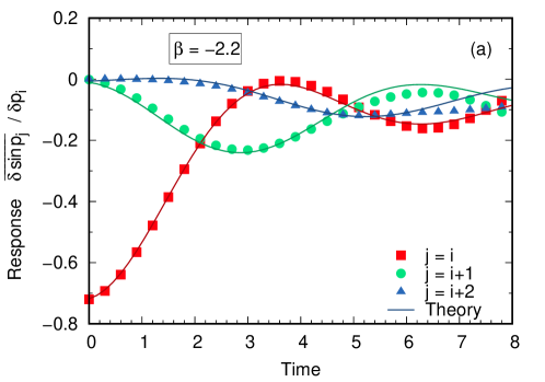
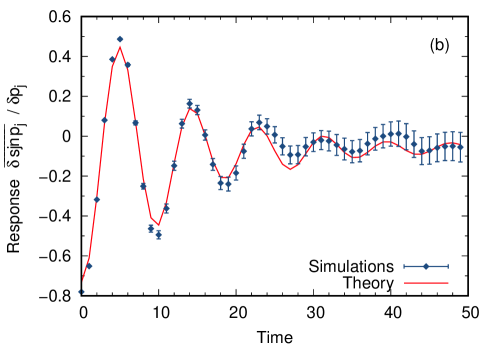
Figure 15: Check of the FDR by a direct computation of the mean response and comparison with the theory in model (159) (panel (a)) and model (129) (panel (b)). In panel (a), the inverse temperature of the considered system is $\beta=-2.2$, $N=128$ and $\delta p_{i}(0)=0.01$, average over $10^{4}$ realizations. As for the plot in panel (b), the parameters are $J=-0.5,\,K=-1.4,\,N=250,\,E/N=1.9$ (corresponding to $\beta\approx-2.6$) and $\delta p_{j}(0)=0.01$. Average over $10^{5}$ realizations. This panel is adapted from Ref. miceli19 .

As a first example of the application of Eq. (168), in Fig. 15(a) we show the effect of a local perturbation in system (159), i.e. a chain of Hamiltonian particles in bounded phase space. At time $t=0$ the momentum of a particle is instantaneously modified,

$$p_{i}\to p_{i}+\delta p_{i}$$ (171)

and the effect on the velocities of the neighbour particles is considered. The FDR reads in this case

$$\overline{\delta\dot{q}_{j}}=\beta\langle\sin(p_{j}(t))\sin(p_{i}(0))\rangle\delta p_{i}\,,$$ (172)

and it is nicely verified by numerical simulations.

In Fig. 15(b) a case with long-range interactions is considered, discussed in Ref. miceli19 . The system is the bounded space-phase Hamiltonian with mean field interactions already introduced in Section IV.3.1. Also in this case an infinitesimal perturbation on the $i$-th momentum induces a response on the velocity given by Eq. (172), where the equilibrium average is now computed according to the mean field Hamiltonian (129). As a side remark, let us notice that this result holds even though, at the considered value of specific energy, there is no equivalence between microcanonical and canonical ensemble in the considered system. Indeed, even if the pdf of the total system is not proportional to $\exp(-\beta\mathcal{H})$ in this case, it can be shown (see Ref. miceli19 ) that the marginal distribution for $p_{i}$ still verifies

$$\rho(p_{i})\propto e^{-\beta[1-\cos(p_{i})]}\,.$$ (173)

This is actually the only requirement to obtain Eq. (172) from the generalized FDR (168), which holds also if the state of the system cannot be described by the canonical ensemble.

VI Non-equilibrium and localization in the DNLS chain

VI.1 Ensemble inequivalence

In Sec. II.5 we have discussed the phenomenology of the DNLS problem and its relation with negative temperatures. In particular, we have pointed out that the existence of negative temperature equilibrium states in the high-energy region of the phase diagram shown in Fig. 3 has been longly debated by several authors. Already in the first paper where this problem was tackled rasmussen00 the authors observed that a thermodynamic approach to the DNLS problem, based on the canonical equilibrium ensemble, yields a negative temperature in the high-energy phase, which contradicts the very existence of a Gibbsian equilibrium measure. Moreover, they guessed that a consistent definition of negative temperatures compatible with a grand-canonical representation could be obtained only by transforming the original short-range Hamiltonian model into a long-range one. Later a thermodynamic interpretation was proposed by Rumpf in the grand-canonical ensemble and he reached the conclusion that negative-temperature states are not compatible with thermodynamic equilibrium conditions R3 ; R4 . More recently, the statistical mechanics of the disordered DNLS Hamiltonian has been analyzed making use of the grand-canonical formalism BM18 : the authors conclude that for weak disorder the phase diagram looks like the one of the non-disordered model, while correctly pointing out that their results apply to the microcanonical case, whenever the equivalence between ensembles could be established. In a more recent paper the thermodynamics of the DNLS model and of its quantum counterpart, the Bose-Hubbard model, has been analyzed by the canonical ensemble CEF . The main claim of these authors is that the Gibbs canonical ensemble is, conceptually, the most convenient one to study this problem and conclude that the high-energy phase is characterized by the presence of non-Gibbs states, that cannot be converted into standard Gibbs states by introducing negative temperatures.

It seems quite hard drawing any clear and consistent conclusion from this contradictory and confused scenario, where it seems that the choice of the adopted statistical ensemble can be made by assuming a priori the preferred one. Conversely, the key question to be answered concerns the equivalence between equilibrium statistical ensembles in the high-energy phase of the DNLS model.

In order to tackle this problem let us first recall some robust and carefully tested numerical results. Extended numerical simulations pointed out that in the high-energy phase the Hamiltonian evolution of an isolated DNLS chain is characterized by the spontaneous formation of long-living multi-breather states, that last over astronomical times franzosi11 ; ICOPP . The microcanonical temperature $T=\Big{(}\frac{\partial S}{\partial E}\Big{)}^{-1}$ (for its rigorous definition see Franzosi ) was found numerically to be negative in this high-energy phase Iubini13 . On the other hand, if one assumes the thermodynamic arguments raised by Rumpf and Newell RN and later by Rumpf R1 ; R2 ; R3 ; R4 , these “negative-temperature” dynamical states should eventually relax to an “equilibrium state”, characterized by an extensive background at infinite temperature with a superimposed localized breather, containing all the excess of energy initially stored in the system. In fact, an equilibrium state is usually expected to occur when entropy is at its maximum value, compatible with the conservation constraints of the model. It is straightforward to realize that this maximum value lies on the line $T=+\infty$ $(\beta=0)$, where the value of the entropy for energies $E>E(T=+\infty)$ is further increased by the “degeneracy” of any giant localized breather collecting a macroscopic fraction of the total energy at any lattice point. As we are going to discuss in the following section, this is exactly what has been observed by simulating the evolution of the DNLS chain by a stochastic dynamics, which conserves energy and total norm Iubini14 ; Iubini17 . We want to point out that this numerical result (obtained for finite chains, as in the studies of deterministic Hamiltonian evolution) cannot be considered as an argument supporting the equivalence of statistical ensembles, for the very reason that in this stochastic dynamics both energy and norm do not fluctuate, as it should happen in a system in contact with standard heat and particle reservoirs. More precisely, the observed equilibrium state could be compatible with a microcanonical measure on the hyper-surface of constant total energy and norm, through a random sampling of the states laying on it. This manifestly has nothing to deal with a grand-canonical measure.

Beyond this heuristic considerations based on numerics, there is a deeper reason to doubt about equivalence of statistical ensembles in the high energy phase. In fact, as pointed out by D. Ruelle in his seminal book  Ruelle , in the presence of condensation phenomena, like the localization of a macroscopic fraction of energy into the breathers of the DNLS system in the high-energy phase, equivalence between statistical ensembles does not apply.

Only recently a consistent thermodynamic interpretation of the phase diagram in Fig. 1 has been proposed GILM1 ; GILM2 . In the low-temperature phase, i.e. in between the line at $T=0$ and the line at $T=+\infty$, equivalence between statistical ensembles is granted, meaning that one can always find a Fenchel-Legendre transform connecting the microcanonical entropy $S(E,A;N)$ to the Gibbs potential ${\mathcal{G}}(T,\mu;N)$ ( $\mu$ is the chemical potential and $N$ is the number of lattice sites, i.e. the spatial extension of the DNLS chain). On the other hand, equivalence between statistical ensembles does not hold in the thermodynamic phase extending above the line at $T=+\infty$, where only a microcanonical description is allowed. For the mathematical details we address the reader to the references GILM1 ; GILM2 . Here we just summarize the main conceptual steps used to reach this conclusion. By elaborating large deviation techniques (e.g., see largedev ) one can compute explicitly the microcanonical entropy $S(E,A;N)$. The passage to the grand-canonical description can be performed by Laplace- transforming $S(E,A;N)$ with respect to $E$ and $A$ by introducing the dual quantities $T$ and $\mu$, respectively. This task is accomplished every time one can find a real solution for both $T$ and $\mu$ in a one-to-one correspondence with $E$ and $A$, respectively. It has been shown that this is always possible for any finite $N$ in the low-energy phase, but in the high-energy phase $E>E(T=+\infty)$ a real solution does not exist for $T$, despite a real solution for $\mu$ still exists for any value of $A$. Moreover, it has been shown that for finite values of $N$ the microcanonical equilibrium states for $E>E(+\infty)$ have a true negative temperature. Only in the thermodynamic limit $N\to+\infty$, while keeping constant the energy and norm densities $E/N$ and $A/N$, the microcanonical equilibrium states boils down to an infinite temperature state with a superimposed giant breather collecting the residual macroscopic fraction of energy $\Delta E=E-E(+\infty)$ GILM2 .

VI.2 Slow relaxation to equilibrium

Besides the properties of the equilibrium state, the nature of the condensation transition in the DNLS equation raises important questions about how the system relaxes to the localized state above the infinite-temperature line. As a matter of fact, the relaxation of a macroscopic DNLS system in the presence of localized states turns out to be extremely slow. In the following, we shall discuss the main mechanisms that are known to be responsible of this slow relaxation. For the sake of simplicity, we will not consider here the effect of intrinsic disorder, thus making reference to the standard DNLS Eq. (36), where the nature of the localization process is exclusively nonlinear. Recent studies on the interplay between nonlinearity and disorder can be found in flach16 ; mallick20 ; kati20 .

Assuming to initialize the system on a generic initial condition far from the final localized state, one can identify two different kinds of sources of slowness, namely entropic and dynamical.

Entropic effects

Entropic effects originate from the presence of entropic barriers in the phase space that slow down the relaxation to equilibrium. Their role is essential for the physics of glassy and disordered systems biroli11 while their influence for the condensation phenomenon of the DNLS equation was studied in Iubini13 ; Iubini14 ; Iubini17 in a purely stochastic version of the model. In these studies it was considered a simplified DNLS model obtained from Eq. (37) by taking the limit of vanishing hopping term. Accordingly, the two conserved quantities of the model read

$$H = \sum_{j=1}^{N}a_{j}^{2}$$

$$A = \sum_{j=1}^{N}a_{j}\,,$$ (174)

where $a_{j}=|z_{j}|^{2}$ are the local norms. One can realize that the equilibrium phase diagram of this simplified model preserves all the relevant features of the DNLS one. In particular the infinite-temperature line separates a low-energy delocalized region from a high-energy localized one Iubini17 ; SEM14 . A stochastic short-range conservative dynamics was defined by introducing local microcanonical Monte-Carlo moves. In detail, given a random triplet of consecutive sites $(j-1,j,j+1)$ and assuming periodic boundary conditions, it is performed a random update of the norms $(a_{j-1},a_{j},a_{j+1})$ such that the total energy and norm of the triplet are conserved Iubini14 .

Above the infinite-temperature line, the microcanonical relaxation dynamics manifest itself in the form of a coarsening of breathers. At early times, several breathers with small amplitude are created, while over longer time scales they are found to progressively disappear. During this process, the average energy of the survived breathers increases until a single breather localizing all the excess energy remains. Overall, the average breather distance $\lambda$ is found to increase subdiffusively as $\lambda=t^{\alpha}$, with $\alpha=1/3$. The physical interpretation of such a subdiffusive coarsening is that breathers exchange energy among themselves diffusively through the background with an effective diffusion constant that scales as $\lambda^{-1}$. As a result, the fewer the breathers are, the slower the relaxation process is.

To summarize, the study of conservative stochastic versions of the DNLS equation unveils the presence of a first source of slowness in the form of a coarsening of localized states. Such an effect is purely entropic and originates from the properties of the two conserved quantities of the model and of the constraint on the positivity of local norms $a_{j}$.

Dynamical effects

Despite its simplicity and analytic tractability GILM1 ; Iubini17 , the uncoupled limit of the DNLS equation is rather peculiar because (i) the original coupling mechanism is replaced by an effective stochastic interaction and (ii) the phase dynamics of the local variables $z_{j}$ does not play any role. When the full (deterministic) DNLS dynamics is considered, an essential physical effect must be taken into account: high-energy breathers are characterized by a large local frequency $\omega_{j}$ which scales as the breather’s local norm $a_{j}$. As a result of this fast rotation, higher breathers are effectively dynamically decoupled from the rest of the system.

The intrinsic dynamical stability of breather states makes the localization process of the full DNLS model even slower. Indeed, microcanonical simulations slightly above the $\beta=0$ line have not shown any evidence of coarsening. Instead, the system was observed to relax on a long-lasting metastable state characterized by a finite and stationary breather density and a negative (Boltzmann) temperature. In practice, a dynamical mechanism prevents breathers from becoming too large. These findings have been confirmed by more recent numerical studies, which identify a subregion of the localized phase where the DNLS dynamics is ergodic mithun18 . Except for this subregion, the nucleation of breather solutions in the localized phase was observed to be compatible with a (weakly) nonergodic dynamics. In this respect, we mention that a similar behaviour was found in related studies of rotor chains and Klein-Gordon lattices, where the concept of dynamical glass was introduced to identify the onset of extremely long ergodization time scales mithun19 ; danieli19 .

The dynamical freezing of relaxation due to breather states in the DNLS equation was studied in detail in ICOPP ; iubini20 in a simplified setup. In particular, it was performed a statistical study of the relaxation of a single breather on a background thermalized at positive temperature. While thermodynamics predicts that the breather needs to disappear at equilibrium rasmussen00 , its average lifetime (i.e. the time needed to be completely absorbed by the background) was found to be exponentially large in the breather initial norm ICOPP . In short, the breather relaxation dynamics was found to be characterized by extremely long “laminar” periods interrupted by sporadic and sudden energy jumps. During the laminar phase, the breather amplitude displays small fluctuations with no clear evidence of specific drifts. A direct measure of a suitable diffusion coefficient reveals that this quantity decreases exponentially with the initial breather norm, in agreement with the evidence of a dynamical freezing mechanism. Energy jumps were found to be correlated to the transient creation of localized dimer states or the occurrence of resonances between the breather and the surrounding background. Both these processes are essentially rare events, whose probability of occurrence was estimated to be exponentially or even super-exponentially small with the breather norm.

The above results bring to the fore several open problems and future perspectives. On the one hand, an exponentially small coupling between breathers and background seems compatible with the absence of a direct numerical observation of the coarsening of breathers. More precisely, one should expect that the dynamical freezing mechanism induces an extremely slow logarithmic coarsening Iubini17 , although no direct evidence has been found. On the other hand, the dynamical origin of the freezing mechanism is not clear at all. In this respect, in ICOPP it was argued that the dynamics is slow because an adiabatic invariant localized on the breather site blocks energy diffusion. An approximate expression of the adiabatic invariant was derived perturbatively at the lowest orders in the inverse breather norm. However, the properties of this adiabatic invariant at higher perturbative orders have still to be explored.

It seems natural to conclude this Section by remarking that the onset of negative-temperature states in the DNLS equation involves a very rich scenario where fundamental aspects of statistical mechanics, dynamics and thermodynamics mix together in a quite uncommon way. Despite for this model negative-temperature states do not exist in equilibrium and in the thermodynamic limit, they turn out to be physically meaningful and observable either as robust equilibrium finite-size effects or as extremely long metastable states. These peculiar features have deep implications also in stationary out-of-equilibrium regimes, as it will be discussed in Section VII.

VII Fourier transport

Among the out-of equilibrium situations which are most commonly found in statistical mechanics, the problem of heat transport along one-dimensional systems has a particular relevance. It is well known that the flux of energy in presence of a temperature gradient is well described, in most systems, by the phenomenological Fourier law

$$\mathbf{J}=-\kappa(T)\nabla T\,,$$ (175)

where $\kappa(T)$ is the conductivity tensor, which is assumed to depend only on temperature; despite its apparent simplicity, a rigorous derivation of Fourier law from first principles is still lacking. The topic was widely studied in recent years by considering many simplified models: an exhaustive account of known results and open questions can be found in Ref. lepri03 ; dhar08 .

A typical scenario is represented by a one-dimensional body whose boundaries are kept at fixed temperatures by thermal baths. If the system is close to equilibrium (i.e., there is only a slight difference between the temperatures of the two baths), $\kappa(T)$ can be approximated by a constant and the resulting temperature profile is linear. In this respect, many questions can be raised when systems which admit also negative temperatures are taken into account. What happens when the body is coupled to a bath with $T>0$ at one end and to a bath with $T<0$ at the other? Does it reach a stationary state with well-defined local temperatures? Is Fourier law still valid in its form (175) even in this case?

In the following we shall first try to answer such questions by reviewing recent results on this topic. In particular we shall focus our attention on a minimalistic spin chain, ruled by a stochastic dynamics which insures local conservation of energy. This simple toy model provides a sketch of the main features of heat transport in presence of negative temperature; other systems are found to be characterized by qualitatively similar properties baldiub .

We will finally consider a more complex situation, i.e. the DNLSE already mentioned in Section II.5 and widely discussed in Section VI. For reasons which will be clarified in the following, in this case it is not possible to couple the system to a negative-temperature bath; however, due to the additional conservation law which characterize this model, it is possible to observe negative temperature locally even if the system is coupled to thermal baths with $\beta\geq 0$. This nontrivial behaviour is discussed in some detail.

VII.1 Simple one-dimensional models

VII.1.1 Spin chain: equilibrium properties

The first model we shall discuss is somehow inspired by the pioneering experiments on nuclear spins performed by Purcell, Pound and Ramsey in the early ’50s and recalled in Sections II.2, III.3.2 and III.3. As already discussed, in that case the spins are subjected to the action of a large external magnetic field, so that the energy of the system is given by Eq. (32). Such relation can be conveniently adimensionalized, yielding

$$\mathcal{H}=-\varepsilon\sum_{n=1}^{N}\sigma_{n}\,,$$ (176)

where $\varepsilon$ is proportional to the intensity of the external field and $\sigma_{n}=\pm 1$ are Ising spins.

Let us recall the basic equilibrium properties of this model. Denoting by $N_{+}$ and $N_{-}=N-N_{+}$ the number of positive and negative spins, respectively, and making use of Stirling’s approximation, total entropy can be written as

$$S(N_{+})=\ln\left(\frac{N!}{N_{+}!N_{-}!}\right)$$ (177)

$$\approx-N_{+}\ln\left(\frac{N_{+}}{N}\right)+N_{-}\ln\left(\frac{N_{-}}{N}\right)+O(\ln N)\,.$$

Defining the density of positive spins

$$p=N_{+}/N\,,$$ (178)

the specific entropy reads then

$$s(p)=-p\ln(p)-(1-p)\ln\left(1-p\right)\,.$$ (179)

In order to infer an explicit expression for temperature, we have to substitute into Eq. (179) the relation between $p$ and the specific energy $e$,

$$e=\varepsilon(1-2p)\,,$$ (180)

as it can be deduced from Eq. (176). The resulting equation

$$s(e,\varepsilon)=-\frac{\varepsilon-e}{2\varepsilon}\ln\left(\frac{\varepsilon-e}{2\varepsilon}\right)-\frac{\varepsilon+e}{2h}\ln\left(\frac{\varepsilon+e}{2\varepsilon}\right)\,$$ (181)

can be derived with respect to $e$, at fixed $\varepsilon$, so to obtain the inverse temperature:

$$\beta(e,\varepsilon)=\frac{\partial s}{\partial e}=\frac{1}{2\varepsilon}\ln\left(\frac{\varepsilon-e}{\varepsilon+e}\right)\,.$$ (182)

The value of $\beta$ tends to $-\infty$ when $e=\varepsilon$ (all spins are positive) and it tends to $+\infty$ when $e=-\varepsilon$ (all spins are negative). The following relation holds between $p$ and $\beta$

$$p=\frac{e^{\beta\varepsilon}}{2\cosh(\beta\varepsilon)}\,,$$ (183)

which is consistent with the statistical interpretation of $p$ as the probability that, at inverse temperature $\beta$, a given spin is positive.

VII.1.2 Spin chain: heat transport

The above recalled properties hold for any spin system at equilibrium, provided that its energy can be written as in Eq. (176). Now we shall focus our attention to the specific model discussed in Ref. baldiub , characterized by a linear geometry. We assume that the spins are placed along a one-dimensional lattice, and energy is locally conserved; in practice this means that when one spin is “flipped”, i.e. it changes its sign, also one of its neighbours, initially with opposite sign, has to flip as well. A simple stochastic dynamics which provides such behaviour is the following. At each time step one of the $2N-2$ oriented pairs of neighbour spins is randomly extracted; if the first spin is positive and the second one is negative, they are both flipped; otherwise, nothing happens. It can be useful to notice that this dynamics can be mapped into an exclusion process such that each positive spin is replaced by a particle carrying an amount of energy equal to $2\varepsilon$, while each negative spin is replaced by a hole. With this analogy it is clear that the local energy flux in the stationary state reads

$$j_{n}=-2\varepsilon\left(p_{n}w_{n\to n+1}-p_{n+1}w_{n+1\to n}\right)\,,$$ (184)

where $p_{n}$ is the stationary probability to find a particle in site $n$, while $w_{n\to k}$ is the transition rate from site $n$ to its neighbour $k$. Assuming that $p_{n}$ and $p_{k}$ are independent, such rate can be written as

$$w_{n\to k}=\frac{1}{\tau}\,\text{Prob}(\,k\text{ empty }|\,n\text{ occupied })\approx\frac{1-p_{k}}{\tau}\,,$$ (185)

where $\tau$ is a typical time of the dynamics.

To study heat transport in this chain, we need to couple its ends to two thermal baths able to keep the local temperatures of the boundaries at fixed values. The simplest way is to extract periodically the value of the rightmost and of the leftmost spin, according to the distribution (183). A natural choice for the rate of such extraction is $1/\tau$.

If a stationary state is reached, due to local conservation of energy, the average energy flux will be constant along the chain; from Eqs. (184) and (185) we obtain in particular

$$p_{n}(1-p_{n+1})-p_{n+1}(1-p_{n})=p_{n}-p_{n+1}=const.\,,$$ (186)

i.e., the probability of finding a positive spin linearly depends on the site position. Assuming that local equilibrium holds, so that we can define a local inverse temperature

$$\beta_{n}=-\frac{1}{2\varepsilon}\ln\left(\frac{1-p_{n}}{p_{n}}\right)\,,$$ (187)

consistently with Eq. (183), we have an explicit expression for the inverse temperature profile along the chain.

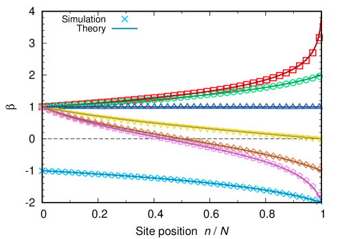
Figure 16: Inverse temperature profiles for the out-of-equilibrium spin chain. Solid lines are computed according to Eq. (187), assuming a linear dependence of $p_{n}$ on the site $n$. Points are results of stochastic numerical simulations as described in the main text. Here $N=128$, $\varepsilon=1$. Figure adapted from Ref. baldiub .

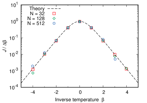
Figure 17: Ratio between heat flux $J$ and inverse temperature difference between the thermal baths. Points are the result of numerical simulations for different values of $N$, with thermal baths at inverse temperature $\beta\pm 0.05$; dashed line is obtained from Eq. (188). Here $\varepsilon=1$. Figure adapted from Ref. baldiub .

In Fig. 16 some of such analytical profiles are compared with the results of numerical simulations, showing a nice agreement. It is worth noticing that, when the temperatures of the two baths have opposite signs, the transition from positive to negative values is realized through a (local) $\beta=0$ state, while the $T$ profile shows a singularity. This observation may seem to imply that Fourier law Eq. (175) does not hold in presence of such a transition; actually, as briefly discussed in Section VII.1.3, a simple change of variable from $T$ to $\beta$ is sufficient to recover the validity of this general principle, as long as close-to-equilibrium cases are considered.

In this respect, it can be useful to consider a slightly different definition of conductivity, i.e. the ratio between the total heat flux $J=N\langle j_{n}\rangle$ (bearing in mind that $\langle j_{n}\rangle$ does not depend on $n$ in the stationary state) and the difference $\Delta\beta$ between the inverse temperatures of the baths. An analytical expression for such ratio can be found in the limit of small $\Delta\beta$ as

$$\frac{J}{\Delta\beta}\approx\frac{\partial J}{\partial\beta}=\frac{N}{\tau}\left(\frac{\varepsilon}{\cosh(\beta\varepsilon)}\right)^{2}\,,$$ (188)

obtained from Eq. (184) using Eqs. 185 and 183. In figure 17 this theoretical curve is compared with the results of numerical simulations. In particular, the “conductivity” $J/\delta\beta$ displays no singularties on the $\beta=0$ state, which corresponds to the condition of maximal transport for fixed differences $\Delta\beta$.

VII.1.3 Other examples and remarks

In Ref. baldiub two additional one-dimensional systems are considered, showing a phenomenology quite similar to that encountered in the case of Ising spins. First, a Hamiltonian chain of the kind (85), already discussed in Section IV.1, is studied; the presence of generalized kinetic terms of the form (87) allows negative temperature, and the local value of $\beta$ at the boundaries can be fixed by mean of stochastic Langevin-like baths (see Section V.2). Then the transport properties of a discrete linear Schrödinger equation model, with Hamiltonian

$$\mathcal{H}=\sum_{n=1}^{N}z_{n}^{*}z_{n+1}+z_{n}z_{n+1}^{*}\,,$$ (189)

are similarly investigated. In both cases, the qualitative scenario already found in the spin chain is confirmed. For all these models, it seems possible to state that:

1. a stationary state is reached, in which local temperatures are well defined and measurable;

2. the presence of negative values of temperature does not contradict the basic principle that heat flows from hot to cold;

3. when the two ends of the chain are kept at fixed temperatures with opposite signs, the $\beta$ profile is continuous, meaning that a part of the chain in which $\beta=0$ locally can be found; this means that the $T$ profile shows a singularity.

The last point may raise some concern. Indeed, it may appear to contradict Fourier’s law as stated in Eq. (175). However, let us remark that if the same law can be written in terms of $\beta$ as well, yielding

$$\mathbf{J}=\tilde{\kappa}(\beta)\nabla\beta\,,$$ (190)

where

$$\tilde{\kappa}(\beta)=\frac{\kappa(1/\beta)}{\beta^{2}}$$ (191)

for $\beta\neq 0$.

Equation (190) implies that, when the difference between the inverse temperatures of the two baths is small and $\tilde{\kappa}(\beta)$ can be reasonably approximated by a constant, the $\beta$ profile should be almost linear. Of course, if such condition is fulfilled and both reservoirs have positive temperature, also the $T$ profile is almost linear, as predicted by the usual formulation of Fourier law (175).

In Ref. baldiub a simple argument is provided in order to explain why $\beta$ is the right variable to consider in this case: the basic idea is that, assuming local equilibrium, the probability to find adjacent regions of the chain with very different values of $\beta$ is very small, and this is also true if $\beta\leq 0$.

VII.2 DNLS equation

When a DNLS chain is put in contact with external reservoirs at its edges, stationary nonequilibrium states are expected to be controlled by suitable gradients of temperature and chemical potential. A first study of the nonequilibrium DNLS equation (36) was done in iubini12 in the positive-temperature region. The related transport of norm and energy was found to be normal (diffusive), with finite Onsager coefficients in the limit of large system sizes. In particular, the presence of non-vanishing off-diagonal Onsager coefficients gives rise to coupled transport with a non-vanishing Seebeck coefficient and related unconventional phenomena such as non-monotonic temperature profiles iubini12 ; iubini16 .

The study of the above setup is crucially founded on the possibility to impose given values of temperature and chemical potential locally by means of suitable models of reservoirs. In this context, it would be tempting to introduce appropriate reservoirs at negative temperature in order to drive the system to the negative-temperature, localized region, as done in Sec. VII.1.3. Unfortunately, this program appears to be inconsistent for the DNLS model because of the nonequivalence of statistical ensembles discussed in Sec. VI.1. Indeed, a naive attempt of thermalization of the DNLS equation with one of the reservoir schemes discussed in Sec. V would result in an unstable dynamics, as shown in Fig. 18. In this example, the interaction with a reservoir at $\beta=-1$ and $\mu=0$ produces a clear exponential divergence of both the total energy $H$ and the total norm $A$, see Eq. (37) and (38). In practice, the system localizes a large amount of energy in increasingly high breather states which grow indefinitely, see the inset for a typical configuration obtained after a time of order $10^{4}$ units.

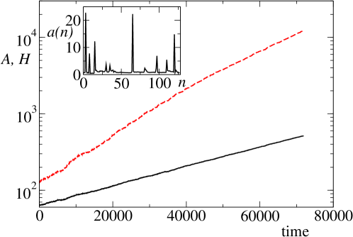
Figure 18: Evolution of the total norm $A$ (black solid line) and total energy $H$ (dashed red line) of a DNLS chain Eq. 36 with $N=128$ lattice sites and $\Lambda=2$ in contact with a grand-canonical Monte-Carlo reservoir at inverse temperature $\beta=-1$ and chemical potential $\mu=0$. Monte-Carlo moves consist in random perturbations of the complex variable $z_{k}\rightarrow z_{k}+\delta$, where $k$ is a randomly selected site of the chain and $\delta$ is extracted from a uniform distribution in the square $[-d:d]\times i[-d:d]$, with $d=0.07$. Monte-Carlo updates occur at random times whose periods $\tau$ are extracted from a Poissonian distribution $P(\tau)\sim\exp(-\tau)$. The inset shows the final norm profile obtained at $t=7.2\cdot 10^{4}$ time units.

These results should clarify that the nonequilibrium setup discussed in Sec. VII.1.3 for negative-temperature Fourier transport can not be applied to the DNLS model in Eq. (36)  If this seems to prevent the study of the response of the system to small negative-temperature unbalances, and thereby the direct measurement of transport coefficients in the negative-temperature region, it should be pointed out that nonequilibrium negative-temperature steady states do exist in the DNLS equation for sufficiently large unbalances. In this respect, in Ref. iubini17entropy it was studied a setup where a DNLS chain is in contact with a positive-temperature reservoir and a pure norm dissipator acting on opposite edges. It was shown that the model can display steady (coupled) transport, with temperature profiles that enter the region of negative absolute temperatures in the central part of the chain, see Fig. 19. Such an unusual behaviour occurs when the temperature of the reservoir $T_{L}$ is large enough ($T_{L}\gtrsim 3$ for the example of Fig. 19) and it is accompanied by non-monotonic temperature profiles, which are therefore qualitatively different from the ones discussed in Sec. VII.1.3. It should be stressed that the corresponding density profiles obtained in iubini17entropy are not localized, despite a part of the system is locally above the $\beta=0$ line of the equilibrium phase diagram (Fig. 3). This feature appears to confirm the relevance of delocalized negative-temperature states found in GILM1 for an isolated DNLS model, at least for large but finite system sizes. When $T_{L}$ is further increased ($T_{L}\simeq 10$), a different transport regime sets up and persistent localized excitations (breather states) are observed to strongly inhibit transport. Indeed, a sort of “thermal wall” (see the orange curve) was observed to segregate an extended positive-temperature profile from an almost empty region close to the dissipator.

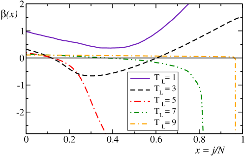
Figure 19: Stationary inverse temperature profiles of a DNLS chain Eq. (36) with $N=4095$ sites and $\Lambda=2$. The parameter $T_{L}$ indicates the different values of boundary temperature imposed by the reservoir placed at the left edge of the chain, with $\mu=0$. The rightmost site is attached to a pure norm dissipator with fixed dissipation rate. Figure adapted from Ref. iubini17entropy . Details of the numerical setup in iubini17entropy .

Despite the above phenomenon requires further investigations and numerical efforts to clarify the role of finite-size effects and the behaviour in the thermodynamic limit, some preliminary considerations can be outlined. According to Ref. iubini17entropy , there is evidence that negative temperatures can arise locally in steady transport setups even when the system interacts with positive-temperature environments. This genuine nonequilibrium mechanism is observed when large unbalances and high temperatures are imposed. Accordingly, the related transport regimes appear to be intrinsically far-from-equilibrium, since a description in terms of linear response coefficients seems to be not feasible. Moreover, signatures of anomalous transport have been reported in this setup, a feature that has been previously observed in similar setups involving purely dissipative boundary conditions iubini14prl .

VIII Conclusions

In this review we have analyzed the statistical properties of systems which admit negative absolute temperature. Although the possibility to have states at negative temperature had been established, even at experimental level, many decades ago, there is still some confusion about the appropriate formalism to use in the macroscopic description of this class of systems, as well as their real physical relevance and the possibility to have a consistent statistical mechanics for them. Going beyond the possible difficulties due to terminology, and some specious arguments, our main aim was a detailed physical discussion of the general theoretical facets of the concept of temperature, and overall an illustration of the way to build an appropriate statistical mechanics description of systems with negative absolute temperature.

We have first reviewed the main phenomenological and theoretical aspects of some systems showing negative temperatures, such as nuclear spins, two-dimensional vortices, lasers, cold atoms and nonlinear discrete Schrödinger equation. All these systems are interesting per se from a physical point of view, and the possibility to observe thermal states which are correctly characterized by a negative-temperature description is an experimental fact.

Starting from the two possible definitions of temperature (Boltzmann vs Gibbs, obtained by using the “surface” or “volume” entropy, respectively) in the well-established framework of equilibrium statistical mechanics, we tried to clarify some subtle aspects related to entropy and its relations with thermodynamics and statistical properties of Hamiltonian systems. In particular we summarized some different points of view about the role of the two possible definitions of temperature with respect to equipartition theorem, adiabatic invariance of the entropy, Helmholtz’s theorem, as well as the problem of thermodynamic cycles. For sure Gibbs formalism shows interesting and relevant properties, which allow, for instance, to establish a rigorous relation between thermodynamics and statistical mechanics even in systems with few degrees of freedom; however, the overall picture emerging from works by many authors indicates that Boltzmann temperature has many advantages when the problem of equilibrium between systems at contact is considered, and it is the only meaningful one when dealing with systems with decreasing density of states.

Our journey, then, crossed the realm of statistical mechanics description of systems with negative absolute temperature. We began with a treatment of the equilibrium case, in particular the problem of the measure of temperature with an appropriate thermometer, which allows for the possibility to establish a zero law even in non standard systems, i.e. systems without the usual quadratic kinetic energy. In addition we analyzed the problem of the ensemble equivalence (and its possible violations), both in systems with short-range and long-range interactions. Then we considered the main topics of the non equilibrium statistical mechanics: the possibility to establish in a consistent way a Langevin equation for the evolution of slow variables, the problem of modeling thermal baths (e.g., for numerical simulation purposes) and the validity of linear response theory. We also discussed the peculiar properties of the discrete nonlinear Schrödinger equation, in which negative temperature states are related to localization and ensemble inequivalence, and the validity of Fourier law for heat transport phenomena in the presence of negative temperature. In all these cases, the negative-temperature description appears consistent with known results of statistical mechanics and the outcomes of numerical simulations.

The take-home message from the large body of works considered in this review appears rather clear and unambiguous: systems with decreasing density of states should not be considered pathological. They can indeed present some non standard features, but it is nevertheless possible to build a consistent macroscopic description both for equilibrium and out-of-equilibrium properties. Such description is a natural generalization of the well-established framework of statistical mechanics, obtained by including also negative values of Boltzmann temperature, and it is in complete agreement with all known experimental results.

Funding

The work of M. Baldovin, R. Livi and A. Vulpiani was supported by the MIUR-PRIN2017 Coarse-grained description for non-equilibrium systems and transport phenomena (CO-NEST).

References

- (1) A. Puglisi, A. Sarracino, A. Vulpiani, Temperature in and out of equilibrium: A review of concepts, tools and attempts, Phys. Rep. 709-710 (2017) 1.
- (2) E. Nagel, The Structure of Science, Hackett Publishing Company, Indianapolis, 1979.
- (3) L. Onsager, Statistical hydrodynamics, Nuovo Cimento Suppl. VI Ser. IX 6 (1949) 279–287.
-
(4)
N. F. Ramsey,
Thermodynamics and