Adaptive and Efficient Model Predictive Control for Booster Re-entry

Nomenclature

$A$  =	open-loop dynamics matrix
$A_{m}$  =	desired closed-loop dynamics matrix
$\Delta A$  =	model mismatch matrix
$B_{m}$  =	matched input gain matrix
$B_{um}$  =	unmatched input gain matrix
$c$  =	aerodynamic reference length, m
$C$  =	output matrix
$C_{m_{\alpha}}$  =	pitch stiffness coefficient, $\text{deg}^{-1}$
$C_{m_{q}}$  =	pitch damping coefficient, $\text{(deg/s)}^{-1}$
$C_{m_{\delta_{e}}}$  =	pitch control effectiveness coefficient, $\text{deg}^{-1}$
$C_{N_{\alpha}}$  =	normal force gradient coefficient, $\text{deg}^{-1}$
$C_{N_{\delta_{e}}}$  =	normal force due to elevator deflection coefficient, $\text{deg}^{-1}$
$f_{1}(x(t),z(t),t))$  =	matched uncertainty
$f_{2}(x(t),z(t),t))$  =	unmatched uncertainty
$F$  =	free-response matrix
$G$  =	forced response matrix
$I_{2}$  =	y component of moment of inertia matrix, $\text{kg m}^{2}$
$K$  =	optimal gain matrix
$m$  =	number of control inputs
$\bar{m}$  =	mass, kg
$n$  =	number of states
$Q$  =	output error weight
$R$  =	control weight
$q$  =	pitch rate, deg/s
$\bar{q}$  =	dynamic pressure, Pa
$\bar{S}$  =	aerodynamic reference area, $\text{m}^{2}$
$S$  =	eigenvectors
$u_{opt}$  =	optimal control input
$u_{ad}$  =	adaptive control input
$V$  =	velocity, m/s
$x$  =	state vector
$x_{z}$  =	internal unmodelled dynamics
$\tilde{x}$  =	state prediction error
$y_{r}$  =	reference command
$\alpha$  =	angle of attack, deg
$\lambda$  =	eigenvalue
$\Phi$  =	state transition matrix
$\omega_{u}$  =	input gain
$||\cdot||_{2}$  =	euclidean norm

1 Introduction

Model predictive control (MPC) is an optimal control strategy where control input calculation is based on minimizing the predicted tracking error over a finite horizon that moves with time. This strategy has an advantage over conventional state feedback and output feedback controllers because it predicts the response of the system, rather than simply reacting to it. Therefore, MPC can offer improved performance in the presence of input and output constraints. Many implementations of MPC on aerospace vehicles appear in literature [1]. Some of these include spacecraft and satellite attitude control [2, 3, 4], spacecraft rendezvous and docking [5], helicopters [6], and atmospheric re-entry [7, 8].

There are many unique challenges associated with the control of hypersonic and supersonic re-entry vehicles, including 1) nonlinear and highly uncertain dynamics, 2) time-varying plant parameters, and 3) fast (and sometimes unstable) open-loop state dynamics, requiring a high control update rate. MPC was applied in simulation for the re-entry X-38 unpowered crew return vehicle (CRV), using quadratic programming at an update rate of 10 Hz [7]. However, the CRV has stable open-loop longitudinal dynamics at high angles of attack [9], allowing for the low update rate. In general, reusable boosters may not have stable re-entry open-loop dynamics [10, 11]. Therefore, a higher control update rate might be required than what is computationally tractable with a conventional constrained quadratic program based MPC.

A number of strategies exist to address the problem of computational tractability in MPC. Explicit MPC involves pre-computing some (or all) of the optimal control solutions and embedding them into multi-dimensional look-up tables for online access [12, 4]. However, this involves a tedious and labour-intensive process of compiling all the required solutions into tabular form. The complexity increases further if the model is time-varying or has uncertain parameters.

A set of algorithms called efficient model predictive control have emerged in recent literature, which reduce the number of prediction points to reduce the computational load [13, 14, 12]. One of these algorithms, called algebraic model predictive control (AMPC), involves using an eigendecomposition to calculate the state transition matrix, resulting in no truncation error regardless of the time step size [13]. Consequently, an absolute minimum of one prediction point may be used without truncation error penalties in the prediction step. For the unconstrained case, quadratic programming is not required, and the optimal control solution for AMPC may be reduced into a closed-form expression analogous to a state feedback controller.

One of the well-understood limitations of all MPC schemes is their reliance on an accurate model, which determines the quality of the predictions, and therefore, the optimal control input computed by the algorithm. The presence of unmodeled nonlinear dynamics, noisy data, as well as aerodynamic and gravimetric uncertainties all contribute to model inaccuracies. This note aims to provide a control scheme that alleviates this reliance on an accurate model by applying an adaptive control augmentation to the AMPC control law. Adaptive MPC has been investigated previously by incorporating a parameter estimation algorithm to identify the model used by the MPC [15, 16, 17, 18]. These studies show that the control performance is initially conservative due to the large parametric uncertainty, but improves over time as the parameter estimates converge to their true values. However, persistent excitation is a requirement for convergence of the parameter estimator.

$\mathcal{L}_{1}$ adaptive control for matched uncertainties has also been combined with MPC and applied to the trajectory tracking problem of a quadrotor, resulting in improved experimental performance compared to non-predictive and non-adaptive approaches [19]. The MPC controller is used to compute the optimal reference command, which is then augmented by the $\mathcal{L}_{1}$ adaptive control law. In the presence of dynamic disturbances, the MPC-$\mathcal{L}_{1}$ controller was able to retain highly accurate tracking performance. Furthermore, the study showed that the $\mathcal{L}_{1}$-augmented non-predictive control schemes had more time delay compared to the MPC-$\mathcal{L}_{1}$ scheme.

Adaptive control methods that utilize an online parameter estimator have severe limitations when applied to hypersonic and supersonic re-entry. These limitations are due to the persistent excitation requirement as well as fast and time-varying system parameters. A study involving system identification methods for adaptive control of a hypersonic glider has shown that the convergence for the parameter estimation algorithm is too slow in the presence of the fast parametric variation in hypersonic flight [20]. $\mathcal{L}_{1}$ adaptive control is the preferred augmentation for several reasons: 1) the transient performance can be known without requiring persistent excitation, 2) decoupling of robustness and adaptation rate allows for fast adaptation, and 3) a bounded time delay margin [21]. For the reasons listed, $\mathcal{L}_{1}$ adaptive control has been implemented on aerospace systems such as quadrotors, aircraft, missiles, and hypersonic vehicles [22, 23, 24, 21, 25].

The main contributions of this note are: 1) Formulation of AMPC to control a linear time-varying (LTV) booster re-entry model, 2) presentation of an adaptive AMPC scheme, combining the AMPC optimal control law with an $\mathcal{L}_{1}$ augmentation for matched and unmatched uncertainties, 3) showing that the closed-form solution in unconstrained AMPC can be exploited to cast the state-space model into a partially closed-loop form amenable to adaptive control synthesis, and 4) showing that the AMPC-$\mathcal{L}_{1}$ scheme outperforms non-adaptive AMPC in off-design conditions.

The note is as follows: Section 2 presents the control methodologies for AMPC and AMPC-$\mathcal{L}_{1}$. In Section 3, simulation results are discussed, and the control schemes are benchmarked against each other. A Monte Carlo analysis and robustness analysis are also conducted. Section 4 details the final conclusions. The booster re-entry model is provided in the Appendix.

2 Controller Design

2.1 Algebraic MPC

AMPC is a model predictive control strategy that utilises an exact solution for the state transition matrix in its prediction step. The unconstrained, single prediction point form of AMPC is used in this study. The full derivation is not provided here, but may be found in [13]. For the unconstrained case, the optimal control law can be obtained by minimizing the cost function with respect to the hypothesized control inputs. The result of the optimization yields the gain matrix acting on the predicted output errors. That optimal gain matrix is

$$K=(G^{T}QG+R)^{-1}G^{T}Q,$$ (1)

where $G$ is the forced response matrix, $Q$ is the weighting matrix penalising predicted output errors, and $R$ is the weighting matrix penalising control inputs. The matrix $K$ is the optimal set of gains acting on the error between the predicted response of the system and the reference command.

The single prediction point AMPC makes the matrices the smallest possible, thereby allowing for the fastest update rates. For a single-input single-output (SISO) system, the predicted error and control activity weights become scalars. For a linear state-space system of the form

$$\dot{x}=Ax+B_{m}u,$$ (2)

the free and forced response matrices are

$$F =C\Phi(\delta t)$$ (3)

$$G =CA^{-1}\Big{(}\Phi(\delta t)-I\Big{)}B_{m},$$ (4)

where $\delta t$ is the prediction time horizon, $A$ is the state dynamics matrix, $B_{m}$ is the control input matrix, $C$ is the output matrix, $F$ is the free-response matrix with $F\in\mathbb{R}^{1\times n}$, and $G\in\mathbb{R}$. The distinctive feature of AMPC is that the state transition matrix $\Phi(\delta t)$ is evaluated by computing the exact matrix exponential. The exact matrix exponential is computed using the eigenvalues and eigenvectors of the state dynamics matrix instead of a Taylor series expansion [13]. For a given time interval, the state transition matrix can be expressed as

$$\Phi(\delta t)=e^{A(\delta t)},$$ (5)

where

$$e^{A(\delta t)}=S\;\text{diag}(e^{\lambda_{1}(\delta t)},\dots,e^{\lambda_{k}(\delta t)})\;S^{-1},$$ (6)

with $S$ defining a set of eigenvectors corresponding to the system eigenvalues $\lambda_{1}$ to $\lambda_{k}$. There is no truncation error in this formulation of the matrix exponential. No approximations are made, as a direct solution of the state transition matrix can be found. Any resulting inaccuracies that may stem from the state transition matrix will therefore only be subject to the precision of the model [13].

The optimal control law is formulated using the optimal gain $K$

$$u_{opt}=K(y_{r}-Fx).$$ (7)

This formulation is used in both the baseline AMPC and AMPC-$\mathcal{L}_{1}$ controllers for the purposes of this study.

Equations (1) to (7) are sufficient if the system under control is LTI. For time-varying systems, $K(t)$, $F(t)$, and $G(t)$ must be re-computed at every control update based on the latest system parameters. That is,

$$F(t) =C\Phi(\delta t,t),$$ (8)

$$G(t) =CA(t)^{-1}\Big{(}\Phi(\delta t,t)-I\Big{)}B_{m}(t),$$ (9)

$$K(t) =\Big{(}G(t)^{T}QG(t)+R\Big{)}^{-1}G(t)^{T}Q.$$ (10)

This produces errors in the AMPC prediction, as the free and forced response matrices are assumed to be constant throughout the prediction horizon, when they are time-varying in reality. These modelling errors result in errors in $A$ and $B_{m}$. However, the rate of variation of the parameters is slow relative to the prediction time horizon. Therefore, the amount of uncertainty throughout the prediction horizon is very small. Furthermore, the $\mathcal{L}_{1}$ adaptive augmentation, which is introduced in the subsequent section, is able to compensate for matched and unmatched uncertainties. The control performance under these assumptions is evaluated in Section 3.

2.2 Algebraic MPC with $\mathcal{L}_{1}$ adaptive augmentation

An $\mathcal{L}_{1}$ adaptive controller with piecewise-constant adaptive law for matched and unmatched nonlinear uncertainties is used as the adaptive augmentation for AMPC [26, 21]. The piecewise-constant adaptive law avoids the risk of numerical stiffness associated with the selection of high adaptive gains in MRAC-type adaptive control schemes.

The AMPC is used to compute the desired closed-loop dynamics $A_{m}$ and the optimal gain $K$, which are both used in the $\mathcal{L}_{1}$ adaptive augmentation. Extensive proofs relating to $\mathcal{L}_{1}$ adaptive architectures are provided in [26] and [27]; therefore, only the main results along with a derivation of the partial closed-loop system using AMPC results will be presented in this section.

The architecture of $\mathcal{L}_{1}$ adaptive controllers consists of a state predictor, an adaptive law, and a control law, as illustrated in Figure 1. The goal of adaptive control is to modify the control law based on the uncertainties in the plant. The state predictor uses the estimated uncertainties and control inputs to predict a future state. The error between the predicted state and the actual state is used in the next adaptive step to drive the adaptive law, which modifies the estimated uncertainties. The control law is then modified based on the estimated uncertainties.

Figure 1: AMPC-$\mathcal{L}_{1}$ architecture for matched and unmatched uncertainties $\hat{\sigma}_{1}(t),\hat{\sigma}_{2}(t)$. The dashed box encloses the $\mathcal{L}_{1}$ adaptive augmentation, which interfaces with AMPC via the desired closed-loop dynamics matrix $A_{m}$, reference command $Ky_{r}$, and state $x(t)$.

2.2.1 Derivation of Partial Closed-loop System

The full control input comprises of the optimal control input computed by AMPC and adaptive component as follows:

$$u(t)=u_{opt}(t)+u_{ad}(t),$$ (11)

where $u_{opt}$ is the optimal control input determined by AMPC and $u_{ad}$ is the adaptive component. Combining Equations (2), (7), and (11) yields

$$\dot{x}(t)=Ax(t)+B_{m}\bigg{(}K\Big{(}y_{r}(t)-Fx(t)\Big{)}+u_{ad}(t)\bigg{)}$$ (12)

which may be placed into the partial closed-loop form

$$\dot{x}(t)=(A-B_{m}KF)x(t)+B_{m}\Big{(}Ky_{r}(t)+u_{ad}(t)\Big{)}.$$ (13)

The optimal AMPC gain matrix $K$ and predicted free-response $F$ is used to make the partial closed-loop system Hurwitz, yielding the desired closed-loop dynamics matrix $A_{m}=A-B_{m}KF$. Furthermore, moving $Ky_{r}$ into the adaptive component yields

$$\dot{x}(t)=A_{m}x(t)+B_{m}u_{ad}(t),$$ (14)

where $u_{ad}$ is the adaptive control component that includes $Ky_{r}$. In the presence of unmodelled nonlinear dynamics, matched and unmatched uncertainties as well as uncertain input gain, Equation (14) becomes

$$\dot{x}(t) =A_{m}x(t)+B_{m}\bigg{(}\omega_{u}u_{ad}(t)+f_{1}\Big{(}x(t),z(t),t\Big{)}\bigg{)}+B_{um}f_{2}\Big{(}x(t),z(t),t\Big{)},\;\;\;\;x(0)=x_{0}$$ (15)

$$z(t) =g_{o}\Big{(}t,x_{z}(t)\Big{)}$$ (16)

$$\dot{x}_{z}(t) =g\Big{(}x_{z}(t),x(t),t\Big{)},\;\;\;\;x_{z}(0)=x_{z0}$$ (17)

$$y(t) =Cx(t)$$ (18)

where $B_{um}$ and $B_{m}$ are the unmatched and matched input gain, respectively. The unmatched input gain, $B_{um}\in\mathbb{R}^{n\times(n-m)}$, is a matrix such that $B_{m}^{T}B_{um}=0$ and $\text{rank}([B_{m}B_{um}])=n$. The terms $f_{1}$ and $f_{2}$ are the matched and unmatched uncertainties, respectively, while $x_{z}$ is the internal unmodelled dynamics. $z$ is the output of the unmodelled dynamics. This adaptive control method operates under a number of assumptions, detailed below [27]. Let $X\triangleq[x^{T},z^{T}]^{T}$ and $f_{i}(t,X)\triangleq f_{i}(t,x,z)$, $i=1,2$.

Assumption 1: Boundedness of the matched ($f_{1}(t,0,0)$) and unmatched ($\bm{f_{2}(t,0,0)}$) uncertainties.

There exists $B_{i}>0$, such that $||f_{i}(t,0)||_{\infty}\leq B_{i}$ holds for all $t\geq 0$ and $i=1,2$.

Assumption 2: Semiglobal Lipschitz condition on $\bm{f_{1}}$ and $\bm{f_{2}}$.

For $i=1,2$ and arbitrary $\delta>0$, there exist positive $K_{1_{\delta}}$, $K_{2_{\delta}}$, such that

$$||f_{i}(t,X_{1})-f_{i}(t,X_{2})||_{\infty}\leq K_{i_{\delta}}||X_{1}-X_{2}||_{\infty},\;\;i=1,2,$$

for all $||X_{j}||_{\infty}\leq\delta,j=1,2,$ uniformly in $t$.

Assumption 3: BIBO stability of unmodelled dynamics.

The $x_{z}$-dynamics are BIBO stable with respect to both initial conditions $x_{z0}$ and input $x(t)$, i.e., there exist $L_{z}$, $B_{z}>0$ such that for all $t\geq 0$

$$||z_{t}||_{\mathcal{L}_{\infty}}\leq L_{z}||x_{t}||_{\mathcal{L}_{\infty}}+B_{z},$$

where $z_{t}$ and $x_{t}$ are $z(t)$ and $x(t)$ evaluated at time $t$.

Assumption 4: Partial knowledge of system input gain.

The system input gain matrix $\omega$ is assumed to be an unknown (nonsingular) strictly row-diagonally dominant matrix with the sign of $\omega_{ii}$ being known. Also, assume that there exists a known compact convex set $\Omega$, such that $\omega\in\Omega\subset\mathbb{R}^{m\times m}$, and that a nominal system input gain $\omega_{0}\in\Omega$ is known.

2.2.2 State Predictor

The state predictor is used to predict the system response based on the current estimates of uncertainties $\hat{\sigma_{1}}$ and $\hat{\sigma_{2}}$. The error in prediction drives the adaptive law, which updates the uncertainty estimates. The state predictor has the form

$$\dot{\hat{x}}(t) =A_{m}\hat{x}(t)+B_{m}\Big{(}u_{ad}(t)+\hat{\sigma}_{1}(t)\Big{)}+B_{um}\hat{\sigma}_{2}(t),\;\;\;\;\hat{x}(0)=x_{0}$$ (19)

where $\hat{\sigma}_{1}(t)$ and $\hat{\sigma}_{2}(t)$ are the current adaptive estimates for the matched and unmatched uncertainties ($f_{1}(x(t),z(t),t))$ and $f_{2}(x(t),z(t),t))$), respectively. For the purposes of this note, the state predictor is implemented in simulation to update the predictions at the same rate as the adaptive law.

2.2.3 Adaptive Law

A piecewise-constant adaptive law, first introduced in [24], is used to update the estimated uncertainties $\hat{\sigma}_{1}(t)$ and $\hat{\sigma}_{2}(t)$. The piecewise-constant update law does not require tuning of an adaptive gain, but rather utilizes the adaptation sampling time $T_{s}$, which may be set arbitrarily small subject only to CPU restrictions. For the $i$th adaptation, the adaptative law is

$$\hat{\sigma}(iT_{s})=-B^{-1}\Phi_{ad}^{-1}(T_{s})\mu(iT_{s}),\;\;\;\;t\in[iT_{s},(i+1)T_{s}],$$ (20)

where

$$\hat{\sigma}(iT_{s}) =\begin{bmatrix}\hat{\sigma}_{1}(iT_{s})\\ \hat{\sigma}_{2}(iT_{s})\end{bmatrix}$$ (21)

$$\Phi_{ad}(T_{s}) \triangleq A_{m}^{-1}(e^{A_{m}T_{s}}-\mathbb{I}_{n}),$$ (22)

$$\mu(iT_{s}) =e^{A_{m}T_{s}}\tilde{x}(iT_{s}),$$ (23)

$$\tilde{x}(t) =\hat{x}(t)-x(t),\;\text{and}$$ (24)

$$B =[B_{m}\;B_{um}].$$ (25)

For an LTI system, Equations (22) and (25) would need only to be computed once as the matrices $A_{m}$ and $B$ are time invariant. In the LTV case, Equations (22) to (25) must be re-computed at every adaptive step as part of the successive linearization process.

2.2.4 Control Law

The matched and unmatched transmission transfer functions are defined in the Laplace domain as

$$H_{m}(s) \triangleq CH_{xm}(s),$$

$$H_{um}(s) \triangleq CH_{xum}(s),$$

where

$$H_{xm}(s) \triangleq(s\mathbb{I}_{n}-A_{m})^{-1}B_{m},\;\text{and}$$

$$H_{xum}(s) \triangleq(s\mathbb{I}_{n}-A_{m})^{-1}B_{um}.$$

These transfer functions are used to formulate the adaptive control law through compensation of the estimated unmatched uncertainty. The adaptive control law in the Laplace domain is

$$u_{ad}(s)=C(s)\Big{(}\hat{\sigma}_{1}(s)+H_{m}^{-1}(s)H_{um}(s)\hat{\sigma}_{2}(s)-Ky_{r}(s)\Big{)}$$ (26)

where $C(s)$ is a user-specified low-pass filter and $K$ is the AMPC optimal gain matrix used to track references. The inverse of the matched transmission, $H_{m}^{-1}(s)$, is unstable for non-minimum phase systems. The angle of the attack dynamics of a fly back booster during re-entry are non-minimum phase. Therefore, the inverse DC gain of $H_{m}(s)$ is used instead to calculate $H_{m}^{-1}(s)H_{um}(s)=-(CA_{m}^{-1}B_{m})^{-1}H_{um}(s)$, a method first proposed in [28]. A property of transfer functions is that the inverse DC gain of $H_{m}(s)$ is the steady-state value of $H_{m}^{-1}(s)$. In the numerical simulation, $H_{um}(s)$ is implemented as a state-space model.

2.2.5 Low-pass Filter and $\mathcal{L}_{1}$-norm sufficient condition

In $\mathcal{L}_{1}$ adaptive control architectures, the low-pass filter is used to decouple the robustness of an adaptive system from the adaptation rate [27]. Therefore, arbitrarily fast adaptations may be specified, subject only to CPU restrictions, while the low-pass filter is designed to bound the stability margins. In this study, the low-pass filter $C(s)$ is a first-order system of the form

$$C(s)=\frac{\omega_{c}}{s+\omega_{c}},$$ (27)

with cutoff frequency chosen based on the trade-off between performance and robustness.

Additionally, the cutoff frequency must be chosen to satisfy the $\mathcal{L}_{1}$-norm condition for closed-loop stability, which is stated as follows [27].

Let $\rho_{in}\triangleq||s(s\mathbb{I}_{n}-A_{m})^{-1}||_{\mathcal{L}_{1}}\rho_{0}$ and let $x_{in}(t)$ be the inverse Laplace transform of $x_{in}(s)\triangleq(s\mathbb{I}_{n}-A_{m})^{-1}$. Since $A_{m}$ is Hurwitz due to AMPC and $x_{0}$ is bounded, then $||x_{in}||_{\mathcal{L}_{1}}\leq\rho_{in}$. Furthermore, define

$$L_{i\delta} \triangleq\frac{\bar{\delta}(\delta)}{\delta}K_{i\bar{\delta}(\delta)},$$ (28)

$$\bar{\delta}(\delta) \triangleq\text{max}\{\delta+\bar{\gamma_{1}},L_{z}(\delta+\bar{\gamma_{1}})+B_{z}\},$$ (29)

where $K_{i\delta}$ is defined in Assumption 2, $\bar{\gamma}_{1}$ is an arbitrarily small positive constant, and $L_{z},B_{z}$ are defined in Assumption 3. For a given $\rho_{0}$, there exists $\rho_{r}>\rho_{in}$ such that the following inequality holds:

$$||G_{m}(s)||_{\mathcal{L}_{1}}+||G_{um}(s)||_{\mathcal{L}_{1}}\ell_{0}<\frac{\rho_{r}-||H_{xm}(s)C(s)K_{g}(s)||_{\mathcal{L}_{1}}||r||_{\mathcal{L}_{\infty}}-\rho_{\text{in}}}{L_{1\rho_{r}}\rho_{r}+B_{0}},$$ (30)

where

$$G_{m}(s) \triangleq H_{xm}(s)\Big{(}\mathbb{I}_{m}-C(s)\Big{)},$$ (31)

$$G_{um}(s) \triangleq\Big{(}\mathbb{I}_{n}-H_{xm}(s)C(s)H_{m}^{-1}(s)C\Big{)}H_{xum}(s),$$ (32)

while

$$\ell_{0}\triangleq\frac{L_{2\rho_{r}}}{L_{1\rho_{r}}},\;\;b_{0}\triangleq\max\bigg{\{}B_{10},\frac{B_{20}}{\ell_{0}}\bigg{\}}.$$

In the AMPC-$\mathcal{L}_{1}$ scheme, $K_{g}(s)=K$ based on the optimal gain calculated using Equation (1).

3 Simulation, Results, and Analysis

3.1 Simulation Setup

This section presents a performance and robustness comparison between AMPC-$\mathcal{L}_{1}$ and baseline, non-adaptive AMPC. The structure of the plant model used for numerical simulation is

$$\dot{x}(t) =\Big{(}A(t)+\Delta A(t)\Big{)}x(t)+B_{m}(t)\omega_{u}\Big{(}u_{ad}(t)-K(t)F(t)x(t)\Big{)}+d(t),$$ (33)

where $\Delta A(t)$ is the plant model mismatch, $d(t)$ is the disturbance vector, and $\omega_{u}$ is the input gain. The plant model mismatch is used to represent uncertainties in aerodynamic parameters while the input gain may be reduced to represent loss of control authority in the actuator loop. For baseline AMPC, $u_{ad}(t)=K(t)y_{r}(t)$.

Several test cases are developed to benchmark the AMPC-$\mathcal{L}_{1}$ against the baseline AMPC in this note. These cases include under nominal conditions, reduced input gain, severe model mismatch, and disturbances as shown in Table 2. The nominal condition in case 1 contains no uncertainties and assumes perfect knowledge of the plant. This is to validate that the AMPC-$\mathcal{L}_{1}$ behaves exactly like non-adaptive AMPC when there are no uncertainties. A Monte Carlo analysis is conducted to obtain a complete view of the controllers’ performance properties under uncertain conditions.

Table 2: Simulation cases for benchmarking AMPC-$\mathcal{L}_{1}$

Simulation	Description
Case 1	Nominal case
Case 2	Reduced input gain ($40\%\;\omega_{u}$)
Case 3	Reduced input gain ($30\%\;\omega_{u}$ and model mismatch)
Case 4	Disturbances
Case 5	Monte Carlo simulation

The AMPC design parameters used for this study are shown in Table 3, while design parameters for $\mathcal{L}_{1}$ adaptive control is shown in Table 4. The simulation is initialized with $\alpha=2$ to represent a post stage separation maneuver, and the control update rate is set to 200 Hz. To compare the control performance of AMPC and AMPC-$\mathcal{L}_{1}$ quantitatively, the tracking error norm is used as a performance metric, defined using

$$||e||_{2}=\sqrt{\int|y_{r}(t)-x(t)|^{2}\text{dt}}.$$ (34)

Table 3: Design parameters for AMPC

Parameter	Description	Value
Q	Tracking error penalty weight	0.99
R	Control activity penalty weight	0.001
$\delta t_{p}$	Prediction horizon	0.5 seconds

Table 4: Design parameters for $\mathcal{L}_{1}$ adaptive control

Parameter	Description	Value
$\omega_{c}$	Low-pass filter cutoff frequency	20 Hz
$\delta t_{ad}$	Adaptive update time step	0.005 seconds

3.2 Discussion of Results

Case 1 - Nominal Conditions:

The results for the nominal case are presented in Figure 2. Under nominal conditions, the controllers generate near-identical control signals, resulting in very similar tracking-error norms of $||e||_{2}=83$ for baseline AMPC and $||e||_{2}=88$ for AMPC-$\mathcal{L}_{1}$.

Firstly, this implies that the modelling errors from assuming that the free and forced response matrices are constant throughout the prediction horizon do not produce significant performance degradation for this system model.

Secondly, this shows that the $\mathcal{L}_{1}$ adaptive augmentation effectively lies dormant when there are negligible uncertainties in the system modelling or input gain. The fly back booster re-entry $\alpha$ commands are accurately tracked by both controllers, showing the viability of AMPC for the longitudinal control of re-entry vehicles.

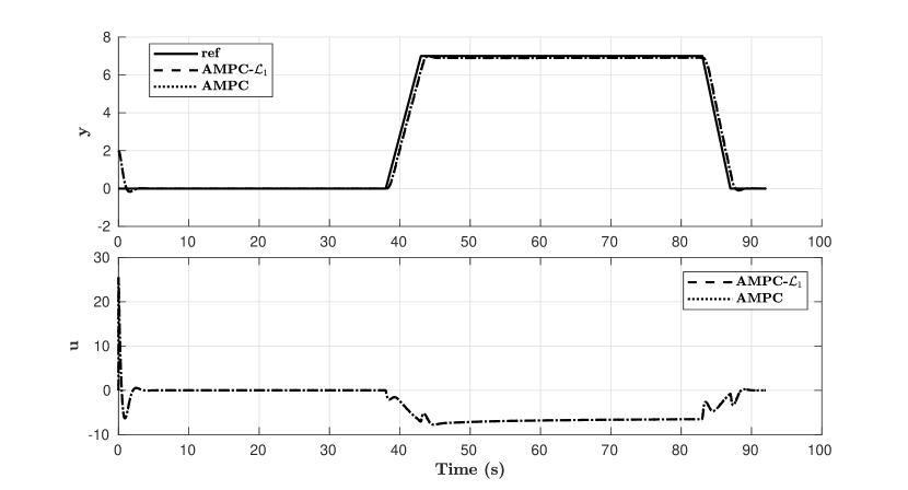
Figure 2: Tracking performance and control activity for case 1. $||e||_{2}=83$ for baseline AMPC and $||e||_{2}=88$ for AMPC-$\mathcal{L}_{1}$. The results are nearly identical, resulting in what appears to be a single dotted, dashed line.

Case 2 - 40% Reduced Input Gain:

The tracking performance and control activity of both controllers under reduced input gain are shown in Figure 3. The steady-state tracking performance of baseline AMPC is degraded, showing a steady-state error of one degree less than the reference command. This is because the AMPC algorithm computes the optimal control without any knowledge of the reduced input gain. Therefore, the AMPC bases its optimization on inaccurate predictions, yielding a control input that would reach the reference set point under nominal conditions, but results in steady-state error under reduced input gain. The transient performance of AMPC is also slightly degraded, with a larger overshoot and settling time compared to the nominal case.

On the other hand, the AMPC-$\mathcal{L}_{1}$ augmented controller retains the good performance from case 1 by adequately compensating for the reduced input gain. This is done by estimating the matched and unmatched uncertainties according to the piece-wise constant adaptive law and compensating for them by requesting more active control according to the control law. The tracking error norm for baseline AMPC is over twice compared to that of AMPC-$\mathcal{L}_{1}$.

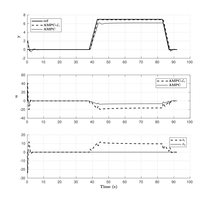
Figure 3: Tracking performance and control activity for case 2. $||e||_{2}=202$ for baseline AMPC and $||e||_{2}=90$ for AMPC-$\mathcal{L}_{1}$. The estimated uncertainties are dominated by the matched uncertainties, compensating for the uncertain input gain.

Case 3 - 30% Reduced Input Gain and Model Mismatch:

To assess the controllers’ performance and robustness under model uncertainties, a severe, time-dependent model mismatch is imposed in the system. This includes reduced pitch rate damping $M_{q}$, reduced static stability $M_{\alpha}$, increased pitch rate to the angle of attack rate mapping, and increased normal force dependence on $\alpha$. This results in the model mismatch matrix

$$\Delta A(t)=\begin{bmatrix}-0.8M_{q}(t)&0.8M_{\alpha}(t)\\ 0.3&0.7\end{bmatrix}.$$ (35)

The performance of both controllers may be seen in Figure 4. There is severe degradation in the performance of the baseline AMPC, marked by oscillatory behaviour in the transient response and a steady-state error of one degree. In contrast, the AMPC-$\mathcal{L}_{1}$ can suppress the oscillations and retain very small steady-state error. The control activity of AMPC-$\mathcal{L}_{1}$ can be seen to be actively compensating for the model mismatch and reduced input gain. Quantitatively, the tracking error norm $||e||_{2}$ of the baseline AMPC controller is over three times higher than the AMPC-$\mathcal{L}_{1}$ controller.

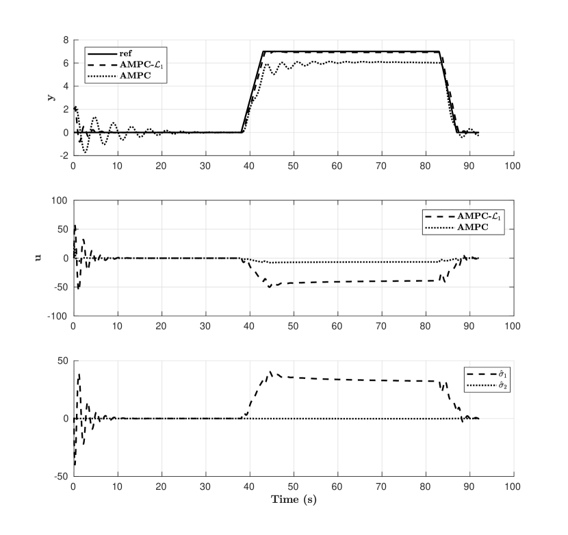
Figure 4: Tracking performance and control activity for case 3. $||e||_{2}=258$ for baseline AMPC and $||e||_{2}=81$ for AMPC-$\mathcal{L}_{1}$. The estimated matched uncertainties dominate the controller for this case.

Case 4 - Disturbances:

To assess the robustness of both controllers to disturbances, a sinusoidal disturbance is imposed on the system defined in Equation (33), defined by

$$d(t)=\begin{bmatrix}0\\ 2\sin(1.5t/\pi)\end{bmatrix}.$$ (36)

The results from imposing the sinusoidal disturbance are shown in Figure 5. These figures show that the AMPC-$\mathcal{L}_{1}$ has a lower tracking error norm than baseline AMPC in the presence of disturbances, evident by the AMPC-$\mathcal{L}_{1}$’s superior suppression of oscillations.

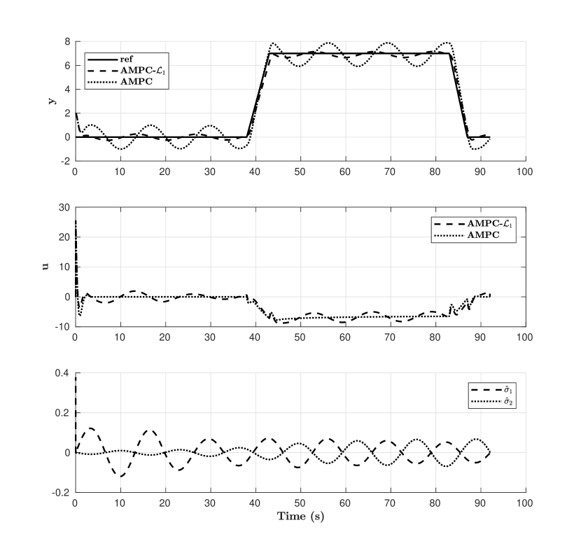
Figure 5: Tracking performance and control activity for case 4. $||e||_{2}=223$ for baseline AMPC and $||e||_{2}=89$ for AMPC-$\mathcal{L}_{1}$. The estimated matched and unmatched uncertainties are equally dominant in the case of disturbance rejection.

Case 5 - Monte Carlo Analysis:

Although cases 1 to 4 clearly show that the AMPC-$\mathcal{L}_{1}$ can provide better control performance when compared to baseline AMPC under some off-design conditions, a Monte Carlo analysis is conducted to establish a more systematic assessment of the controllers’ performance under uncertain conditions. The uncertain parameters are assumed to be normally distributed, with standard deviations shown in Table 5.

Table 5: Uncertain parameters for Monte Carlo simulation

Uncertain Parameters	Description	Standard Deviation
$\delta M_{q}$	Pitch damping	$\sigma(M_{q})=0.25M_{q}$
$\delta M_{\alpha}$	Pitch stiffness	$\sigma(M_{\alpha})=0.25M_{\alpha}$
$\delta\dot{\alpha}_{q}$	Pitch rate to the angle of attack rate map	$\sigma(\dot{\alpha}_{q})=0.25\dot{\alpha}_{q}$
$\delta N_{\alpha}$	Normal force gradient	$\sigma(N_{\alpha})=0.25N_{\alpha}$
$\omega_{u}$	Input gain	$\sigma(\omega_{u})=0.2$

By using the probability distribution from Table 5, one hundred stochastic simulations were computed for both baseline AMPC and AMPC-$\mathcal{L}_{1}$ controllers. The same uncertainties were used to calculate the responses of both control schemes. From the simulation results overlayed in Figures 6 and 7, it is apparent that baseline AMPC has a larger tracking error mean and standard deviation. The means of the tracking error 2-norm for baseline and adaptive AMPC are 97 and 90, respectively, while the standard deviations are 29.1 and 8.0, respectively.

The initial step response is similar for both schemes, but the AMPC-$\mathcal{L}_{1}$ exhibits consistently superior performance in the ramp response from $t=40s$ to $t=90s$. While the baseline AMPC results show a spread of steady-state errors resulting from the parametric uncertainty, the AMPC-$\mathcal{L}_{1}$ can adapt the control signal to account for the model mismatch and uncertain input gain.

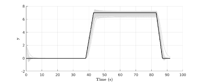
Figure 6: Baseline AMPC overlaid Monte Carlo results

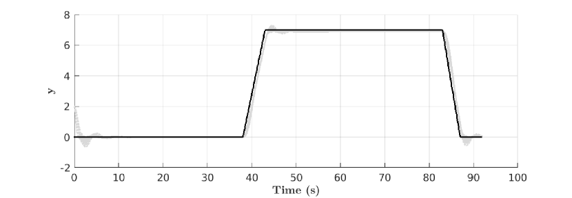
Figure 7: AMPC-$\mathcal{L}_{1}$ overlaid Monte Carlo results

3.3 Robustness Analysis

AMPC Robustness Margins:

In unconstrained AMPC, an optimal gain matrix is computed according to the Equation (1). This allows LTI robustness metrics to be applied to the resulting closed-loop system. However, the booster re-entry model is an LTV system. Therefore, LTI models are generated at various operating conditions for the computation of phase and gain margins. The gain and phase margins along the re-entry trajectory are shown in Table 6.

Table 6: LTI robustness margins for AMPC

Mach	Altitude (m)	Phase Margin (∘)	Gain Margin
5	26,000	125	$\infty$
4	25,000	126	$\infty$
3	23,000	125	$\infty$
2	17,000	$\infty$	$\infty$
1	13000	$\infty$	$\infty$

Time Delay Margins:

For adaptive controllers with nonlinear adaptive laws, phase and gain margins are unsuitable as a robustness metric. A commonly used robustness metric for Model Reference Adaptive Controllers (MRAC) is the time delay margin (TDM). The TDM is the time delay required to render the closed-loop system unstable. Although an analytical method for computing TDM has not yet been derived for this particular $\mathcal{L}_{1}$ adaptive control scheme, the TDM may be computed numerically by gradually increasing the time delay margin until the closed-loop system exhibits signs of instability.

The TDM values are shown in Table 7. It is clear that the $\mathcal{L}_{1}$ adaptive augmentation has severely reduced the TDM of the standard AMPC. This is an expected result, due to the trade-offs associated with robustness and performance. For $\mathcal{L}_{1}$ adaptive control architectures, this trade-off is managed by choosing the cut-off frequency associated with the low-pass filter $C(s)$. Choosing a lower cut-off frequency reduces performance but increases TDM, which will remain bounded regardless of the adaptation rate, allowing for adaptive updates at arbitrarily high frequencies.

Table 7: Time delay margins for AMPC and AMPC-$\mathcal{L}_{1}$ controllers

Mach	Altitude (m)	AMPC (ms)	AMPC-$\mathcal{L}_{1}$ (ms)
5	26,000	300	67
4	25,000	300	67
3	23,000	310	67
2	17,000	280	64
1	13000	287	65

3.4 Computational Performance

One of the claims in this note is that AMPC and AMPC-$\mathcal{L}_{1}$ using single-point prediction are more computationally efficient than conventional constrained MPC solved using quadratic programming. To verify the computational performance of baseline AMPC and AMPC-$\mathcal{L}_{1}$, the computational load of these controllers are benchmarked against conventional MPC. All computations have been performed using MATLAB on an Intel Core i7-8550U CPU @ 1.80GHz with 8GB RAM.

For conventional MPC, an interior point method was used to solve the quadratic program. The state transition matrix was computed using a 5th order Taylor series expansion. For AMPC, the eigendecomposition method was used to evaluate the state transition matrix. A single AMPC control update includes the computation of Equations (6), (1), (3), and (4). For AMPC-$\mathcal{L}_{1}$, the state predictor, adaptive law, and control laws are computed in addition to the calculations required by baseline AMPC. These include Equations (19), (20)-(25), and (26).

The required computation times for each controller to compute a single control update are tabulated in Table 8. Compared to conventional MPC with 10 prediction points, performing a single AMPC update is approximately 15 times faster. With an $\mathcal{L}_{1}$ augmentation, the computational load is more than baseline AMPC, but is still approximately 10 times faster than conventional MPC with 10 prediction points.

Table 8: Comparison of computational load

Control scheme	Time for single control update (s)	Prediction points
MPC	0.0208	10
MPC	0.0073	5
AMPC	0.0013	1
AMPC-$\mathcal{L}_{1}$	0.0022	1

4 Conclusions

In this note, a novel adaptive and efficient model predictive control scheme for use at high update rates has been developed and applied to an LTV fly back booster re-entry model in simulation studies. The AMPC relies on the accurate computation of the state transition matrix via an eigendecomposition to utilize only a single prediction point and does not require any pre-computed solutions. However, the control performance of baseline AMPC degrades in the presence of model mismatch and disturbances. A comparative study between the baseline AMPC and AMPC-$\mathcal{L}_{1}$ controllers has shown that the AMPC-$\mathcal{L}_{1}$ yields consistently better performance than the baseline in the presence of reduced input gain, model mismatch, and disturbances, based on the tracking error 2-norm. Moreover, the AMPC-$\mathcal{L}_{1}$ has exhibited desirable suppression of oscillations and eliminated steady-state error with the cost of a drastically reduced time delay margin. The trade-off between performance and robustness is managed by selecting the cut-off frequency associated with the $\mathcal{L}_{1}$ adaptive control low-pass filter. Future work would include hardware-in-the-loop experiments to verify that the proposed controller is computationally feasible on existing embedded systems.

Appendix

4.1 Booster Re-entry Nominal Trajectory

In this study, an LTV model is used to design the baseline and augmented AMPC controllers. To derive the LTV model, a nominal trajectory of the booster is utilized to generate the time evolution of the aerodynamic derivatives and velocity, which form the basis of the LTV state-space model described in the subsequent section. The booster model used to generate the LTV model is a reusable launch vehicle first stage concept with tail-fins for re-entry control [29]. The re-entry trajectory occurs following stage separation (see Figure 8). The re-entry starts at Mach 5, 26000 km altitude with a ballistic phase, regulating $\alpha$. A pull up maneuver is initiated at $t=38$ seconds in the form of a ramp $\alpha$ command. The maneuver ends at $t=83$ seconds with a down ramp command, shown in Figure 9. The time-varying aerodynamic derivatives to be used in the LTV model are shown in Figure 10.

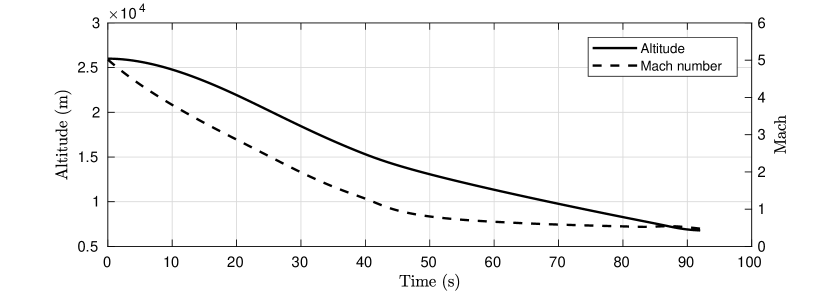
Figure 8: Nominal booster re-entry trajectory

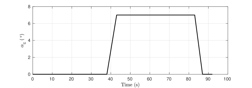
Figure 9: Angle of attack command schedule for pull up maneuver

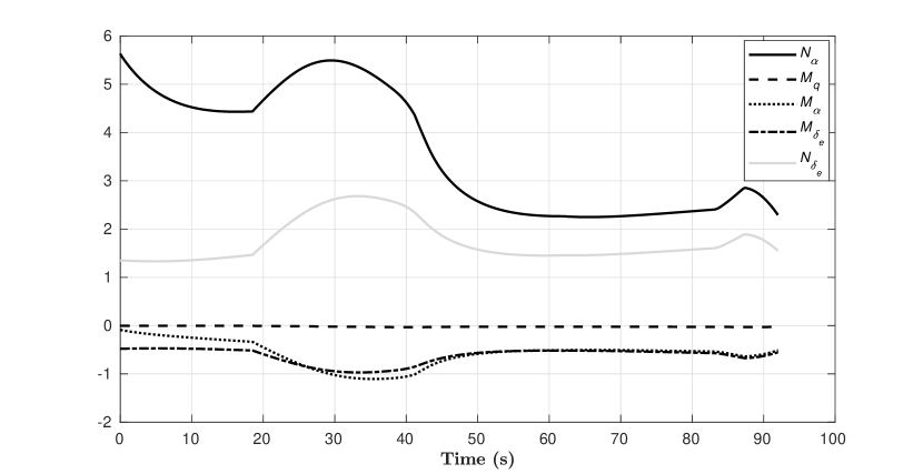
Figure 10: Time evolution of longitudinal aerodynamic derivatives used for the LTV model

4.2 Linearized Longitudinal Dynamics

An angle of attack controller is required to track the commands shown in Figure 9. This section presents a brief description of longitudinal dynamics along with an LTV model, which is used for control synthesis. The longitudinal motion of aerodynamic vehicles consists of two modes: 1) short period oscillation, which involves high-frequency oscillation, and 2) phugoid, the low-frequency mode. When the phugoid mode is neglected, the aerodynamic derivatives that govern the short period longitudinal motion are pitch stiffness $C_{m_{\alpha}}$, pitch damping $C_{m_{q}}$, and normal force gradient $C_{N_{\alpha}}$. The control authority of the elevators is captured in the derivatives $C_{m_{\delta_{e}}}$ and $C_{N_{\delta_{e}}}$. The linearized, short period angle of attack dynamics are

$$\dot{x}(t)=A(t)x(t)+B_{m}(t)u(t) =\begin{bmatrix}\dot{q}(t)\\ \dot{\alpha}(t)\end{bmatrix}=\begin{bmatrix}M_{q}(t)&M_{\alpha}(t)\\ \dot{\alpha}_{q}&-N_{\alpha}(t)/V(t)\end{bmatrix}\begin{bmatrix}q(t)\\ \alpha(t)\end{bmatrix}+\begin{bmatrix}M_{\delta_{e}}(t)\\ \frac{-N_{\delta_{e}}(t)}{V(t)}\end{bmatrix}u(t)$$ (37)

$$y(t)=Cx(t) =\begin{bmatrix}0&1\end{bmatrix}\begin{bmatrix}q(t)\\ \alpha(t)\end{bmatrix},$$ (38)

where

$$M_{\alpha}=\frac{\bar{q}\bar{S}c}{I_{2}}C_{m_{\alpha}},\quad N_{\alpha}=\frac{\bar{q}\bar{S}}{\bar{m}}C_{N_{\alpha}},\quad M_{q}=\frac{\bar{q}\bar{S}c^{2}}{2I_{2}V}C_{m_{q}},\quad M_{\delta_{e}}=\frac{\bar{q}\bar{S}c}{I_{2}}C_{m_{\delta_{e}}},\;N_{\delta_{e}}=\frac{\bar{q}\bar{S}}{\bar{m}}C_{N_{\delta_{e}}}.$$

The parameter $\dot{\alpha}_{q}$ is the pitch rate to the angle of attack map, which is assumed to be one-to-one nominally. Aerospace vehicles have highly nonlinear and time-varying plant parameters. Therefore, an LTV model is used for simulation in this study, where parameters of $A(t)$ and $B_{m}(t)$ are scheduled with respect to time according to the nominal trajectory described in the previous section. However, successive linearization is used with an LTI model for the MPC online optimal control computation. Therefore, the plant parameters are updated according to the current flight condition.

References

- Eren et al. [2017] Eren, U., Prach, A., Koçer, B. B., Raković, S. V., Kayacan, E., and Açıkmeşe, B., “Model Predictive Control in Aerospace Systems: Current State and Opportunities,” Journal of Guidance, Control, and Dynamics, Vol. 40, No. 7, 2017, pp. 1541–1566. 10.2514/1.g002507.
- Chen and Wu [2011] Chen, X., and Wu, X., “Design and Implementation of Model Predictive Control Algorithms for Small Satellite Three-axis Stabilization,” 2011 IEEE International Conference on Information and Automation, IEEE, 2011, pp. 666–671. 10.1109/ICINFA.2011.5949077.
- Wood and Chen [2008] Wood, M., and Chen, W. H., “Model Predictive Control of Low Earth-orbiting Satellites using Magnetic Actuation,” Proceedings of the Institution of Mechanical Engineers, Part I: Journal of Systems and Control Engineering, Vol. 222, No. 6, 2008, pp. 619–631. 10.1243/09596518JSCE505.
- Hegrenæs et al. [2005] Hegrenæs, Ø., Gravdahl, J. T., and Tøndel, P., “Spacecraft Attitude Control using Explicit Model Predictive Control,” Automatica, Vol. 41, No. 12, 2005, pp. 2107–2114. 10.1016/j.automatica.2005.06.015.
- Weiss et al. [2015] Weiss, A., Baldwin, M., Erwin, R. S., and Kolmanovsky, I., “Model Predictive Control for Spacecraft Rendezvous and Docking: Strategies for Handling Constraints and Case Studies,” IEEE Transactions on Control Systems Technology, Vol. 23, No. 4, 2015, pp. 1638–1647. 10.1109/TCST.2014.2379639.
- Ngo and Sultan [2016] Ngo, T. D., and Sultan, C., “Model Predictive Control for Helicopter Shipboard Operations in the Ship Airwakes,” Journal of Guidance, Control, and Dynamics, Vol. 39, No. 3, 2016, pp. 574–589. 10.2514/1.G001243.
- Van Soest et al. [2006] Van Soest, W. R., Chu, Q. P., and Mulder, J. A., “Combined Feedback Linearization and Constrained Model Predictive Control for Entry Flight,” Journal of Guidance, Control, and Dynamic, Vol. 29, No. 2, 2006, pp. 427–434. 10.2514/1.14511.
- Pascucci et al. [2015] Pascucci, C. A., Bennani, S., and Bemporad, A., “Model Predictive Control for Powered Descent Guidance and Control,” 2015 European Control Conference (ECC), IEEE, 2015, pp. 1388–1393. 10.1109/ECC.2015.7330732.
- Horvath et al. [2004] Horvath, T. J., Berry, S. A., Merski, N. R., and Fitzgerald, S. M., “X-38 Experimental Aerothermodynamics,” Journal of Spacecraft and Rockets, Vol. 41, No. 2, 2004, pp. 272–292. 10.2514/1.9198.
- Eggers [2003] Eggers, T., “Aerodynamic Behaviour of a Liquid Fly-back Booster in Transonic Cruise Flight,” 21st AIAA applied aerodynamics conference, 2003, p. 3422. 10.2514/6.2003-3422.
- Chai et al. [2017] Chai, J., Smart, M. K., Forbes-Spyratos, S., and Kearney, M., “Fly Back Booster Design for Mach 5 Scramjet Launch,” 68th International Astronautical Congress, International Astronautical Federation, 2017, pp. 1–11.
- Lamburn et al. [2014] Lamburn, D. J., Gibbens, P. W., and Dumble, S. J., “Efficient Constrained Model Predictive Control,” European Journal of Control, Vol. 20, No. 6, 2014, pp. 301–311. 10.1016/j.ejcon.2014.08.001.
- Gibbens and Medagoda [2011] Gibbens, P. W., and Medagoda, E. D. B., “Efficient Model Predictive Control Algorithm for Aircraft,” Journal of Guidance, Control, and Dynamics, 2011. 10.2514/1.52162.
- Abdolhosseini et al. [2013] Abdolhosseini, M., Zhang, Y. M., and Rabbath, C. A., “An Efficient Model Predictive Control Scheme for an Unmanned Quadrotor Helicopter,” Journal of Intelligent and Robotic Systems: Theory and Applications, Vol. 70, No. 1-4, 2013, pp. 27–38. 10.1007/s10846-012-9724-3.
- Fukushima et al. [2007] Fukushima, H., Kim, T.-H., and Sugie, T., “Adaptive Model Predictive Control for a Class of Constrained Linear Systems based on the Comparison Model,” Automatica, Vol. 43, No. 2, 2007, pp. 301–308. 10.1016/j.automatica.2006.08.026.
- Adetola et al. [2009] Adetola, V., DeHaan, D., and Guay, M., “Adaptive Model Predictive Control for Constrained Nonlinear Systems,” Systems & Control Letters, Vol. 58, No. 5, 2009, pp. 320–326. 10.1016/J.SYSCONLE.2008.12.002.
- Kayacan et al. [2018a] Kayacan, E., Young, S. N., Peschel, J. M., and Chowdhary, G., “High-precision control of tracked field robots in the presence of unknown traction coefficients,” Journal of Field Robotics, Vol. 35, No. 7, 2018a, pp. 1050–1062. 10.1002/rob.21794, URL https://onlinelibrary.wiley.com/doi/abs/10.1002/rob.21794.
- Kayacan et al. [2018b] Kayacan, E., Zhang, Z., and Chowdhary, G., “Embedded High Precision Control and Corn Stand Counting Algorithms for an Ultra-Compact 3D Printed Field Robot,” Proceedings of Robotics: Science and Systems, Pittsburgh, Pennsylvania, 2018b. 10.15607/RSS.2018.XIV.036.
- Pereida and Schoellig [2018] Pereida, K., and Schoellig, A. P., “Adaptive Model Predictive Control for High-Accuracy Trajectory Tracking in Changing Conditions,” IEEE International Conference on Intelligent Robots and Systems, 2018, pp. 7831–7837. 10.1109/IROS.2018.8594267.
- Creagh et al. [2011] Creagh, M., Kearney, M., and Beasley, P., “Adaptive Control for a Hypersonic Glider using Parameter Feedback from System Identification,” AIAA Guidance, Navigation, and Control Conference, 2011, p. 6230. 10.2514/6.2011-6230.
- Banerjee et al. [2015] Banerjee, S., Wang, Z., Baur, B., Holzapfel, F., Che, J., and Cao, C., “ Adaptive Control Augmentation for the Longitudinal Dynamics of a Hypersonic Glider,” Journal of Guidance, Control, and Dynamics, Vol. 39, No. 2, 2015, pp. 275–291. 10.2514/1.g001113.
- Pereida et al. [2019] Pereida, K., Kooijman, D., Duivenvoorden, R. R., and Schoellig, A. P., “Transfer Learning for High-precision Trajectory Tracking through Adaptive Feedback and Iterative Learning,” International Journal of Adaptive Control and Signal Processing, Vol. 33, No. 2, 2019, pp. 388–409. 10.1002/acs.2887.
- Grøndahl [2011] Grøndahl, M. S., “ Adaptive Control,” Masters thesis, University of Oslo, Oslo, 2011.
- Cao and Hovakimyan [2009] Cao, C., and Hovakimyan, N., “ Adaptive Output-Feedback Controller for Non-Strictly-Positive-Real Reference Systems: Missile Longitudinal Autopilot Design,” Journal of Guidance, Control, and Dynamics, Vol. 32, No. 3, 2009, pp. 717–726. 10.2514/1.40877.
- Banerjee [2016] Banerjee, S., “ Adaptive Control Augmentation for a Hypersonic Glider,” Phd thesis, University of Queensland, 2016. 10.14264/uql.2016.102.
- Xargay et al. [2014] Xargay, E., Hovakimyan, N., and Cao, C., “ Adaptive Controller for Multi-input Multi-output Systems in the Presence of Nonlinear Unmatched Uncertainties,” Proceedings of the 2010 American Control Conference, 2014, pp. 874–879. 10.1109/acc.2010.5530686.
- Hovakimyan and Cao [2011] Hovakimyan, N., and Cao, C., Adaptive Control Theory : Guaranteed Robustness with Fast Adaptation, SIAM, Philadelphia, 2011.
- Che and Cao [2012] Che, J., and Cao, C., “ Adaptive Control of System With Unmatched Disturbance By Using Eigenvalue Assignment Method,” Proceedings of the IEEE Conference on Decision and Control, , No. 2, 2012, pp. 4823–4828. 10.1109/CDC.2012.6426412.
- Chai et al. [2018] Chai, J., Smart, M. K., and Kearney, M., “Re-entry Dynamics and Control of Pivot Wing Fly Back Boosters,” 2018 AIAA SPACE and Astronautics Forum and Exposition, 2018, p. 5400. 10.2514/6.2018-5400.