Revisiting Self-Supervised Monocular Depth Estimation

Abstract

Self-supervised learning of depth map prediction and motion estimation from monocular video sequences is of vital importance—since it realizes a broad range of tasks in robotics and autonomous vehicles. A large number of research efforts have enhanced the performance by tackling illumination variation, occlusions, and dynamic objects, to name a few. However, each of those efforts targets individual goals and endures as separate works. Moreover, most of previous works have adopted the same CNN architecture, not reaping architectural benefits. Therefore, the need to investigate the inter-dependency of the previous methods and the effect of architectural factors remains. To achieve these objectives, we revisit numerous previously proposed self-supervised methods for joint learning of depth and motion, perform a comprehensive empirical study, and unveil multiple crucial insights. Furthermore, we remarkably enhance the performance as a result of our study—outperforming previous state-of-the-art performance.

1 Introduction

Accurate estimation of 3D structure (e.g., dense depth map) and camera motion plays a crucial role in computer vision—since it provides key grounds for a wide range of tasks in robotics, autonomous vehicles and augmented reality. Among various sensing modalities for the estimation such as LiDAR [35] and stereo camera [10], monocular cameras are drawing increasing attention due to their cost-efficiency and easy-to-deploy nature. Traditional approaches identify the same points in consecutive image frames for the estimation, which demands a lot of manual feature engineering [12]. Recently, the field is moving towards deep learning [11]. Deep neural networks learn the estimation from data without manual feature engineering and display superior performance.

In the early stage, fully-supervised methods for depth learning from single images using neural networks have emerged [6]. However, the scarcity of datasets with ground-truth for supervision signals has triggered the development of self-supervised methods. Self-supervised learning methods jointly learn depth and motion from monocular video sequences by utilizing geometric constraints as the source of supervision signals [58]. The supervision signals come from projecting temporal frames onto nearby frames using the estimated depth and motion, reconstructing the original frames from nearby frames, and enforcing photometric consistency over the reconstructed frames.

Contemporary approaches of self-supervised monocular depth and motion learning aim to tackle a set of issues to enhance the performance: depth representation [58, 11, 32], illumination variation [10, 54], occlusion induced by view variation [11, 12] and dynamic objects [33, 32]. These issues hinder the learning process as they restrict neural networks from optimally processing information or violate the assumptions implicitly imposed by the geometric constraints such as the static scene or the Lambertian surface assumptions. Although prior works have dramatically enhanced the performance compared to the early works, contemporary research on self-supervised monocular depth and motion learning possesses two main drawbacks:

• Each of the research efforts stands as a separate work and the inter-dependency between them is not well known. As a result, the research on self-supervised depth and motion learning has not yet fully achieved the potential synergies between proposed methods.

• Conventional works, in general, have adopted the identical CNN architecture for a fair comparison of proposed learning methods. Consequently, the need to investigate the effect of architectural factors and reap architectural benefits remains.

To overcome the limitations mentioned above, we propose to have a closer look at potential synergies between various depth and motion learning methods and CNN architectures. For this, we revisit a notable subset of previously proposed learning approaches and categorize them into four classes: depth representation, illumination variation, occlusion and dynamic objects. Next, we design a comprehensive empirical study to unveil the potential synergies and architectural benefits. To cope with the large search space, we take an incremental approach in designing our experiments. As a result of our study, we uncover a number of vital insights. We summarize the most important as follows: (1) choosing the right depth representation substantially improves the performance, (2) not all learning approaches are universal, and they have their own context, (3) the combination of auto-masking and motion map handles dynamic objects in a robust manner, (4) CNN architectures influence the performance significantly, and (5) there would exist a trade-off between depth consistency and performance enhancement. Moreover, we obtain new state-of-the-art performance in the process of performing our study.

2 Related Works

In this section, we review previous research outcomes relevant to our study. We discuss the main ideas of previous works and highlight the novelty of them compared to conventional methods.

2.1 Self-Supervised Depth Estimation

Monocular Depth Estimation. Since the estimation of depth from monocular images is an inherently ill-posed problem, early works have focused on learning the estimation with ground-truth depth labels [6]. Nonetheless, the expensive cost of collecting ground-truth depth labels has led to the development of self-supervised monocular depth estimation [58]. In self-supervised monocular depth estimation, two CNNs learn to estimate depth and relative camera motion. Supervision signals come from warping temporal image frames onto nearby frames using the estimated depth and motion, reconstructing the original frames from nearby frames and enforcing photometric consistency. This photometric consistency implicitly assumes that scenes are static (rigid) and Lambertian. Thus, violation of the assumptions—which frequently occurs in natural scenes—degrades the depth estimation performance. Various research teams have attempted to enhance the monocular depth estimation performance in real-world scenes. Mahjourian et al. leveraged the point cloud alignment in addition to the photometric consistency constraint [37]. Casser et al. utilized semantic information to handle 3D object motion [3]. Bian et al. pursued scale consistency to overcome the scale ambiguity problem of monocular depth and motion estimation [1]. Godard et al. reduced the performance gap between stereo and monocular self-supervised depth estimation by proposing multi-scale estimation and per-pixel minimum reprojection loss [11]. Nevertheless, these approaches still need to resolve the gradient deterioration problem caused by dynamic objects in the scenes.

Handling of Dynamic Objects. One of the challenges self-supervised depth and motion estimation faces is the performance impairment due to dynamic objects. Dynamic objects hinder the evaluation of the photometric consistency constraint, corrupt supervision signals and deteriorate the performance. One straightforward approach is incorporating semantic information and handling dynamic objects. SIGNet fuses semantic information from pre-trained networks to make depth and flow predictions consistent over dynamic regions of the scene [38]. Casser et al. and Godon et al. utilized instance segmentation masks from pre-trained segmentation networks to handle 3D object motion [3, 12]. Furthermore, learning optical flow as an auxiliary task would enhance the depth estimation performance. Early works introducing unsupervised learning of optical flow trained CNNs with image synthesis and local flow smoothness [19, 44]. Later, researchers integrated the optical flow learning into the depth estimation learning [56, 60, 34]. Recently, Li et al. proposed the group smoothness loss and the $L_{1/2}$ sparsity loss for learning dynamic object masks in a self-supervised manner [32].

Uncertainty Estimation. Proper quantification of uncertainty prevents overconfident incorrect predictions and aids the process of decision making in real-world computer vision applications [30]. Uncertainties mainly arise from two sources: input data (aleatoric uncertainty) or model itself (epistemic uncertainty) [21]. The noise in data—generally originates from sensor imperfection—causes aleatoric uncertainty while the limited model capacity or unbalanced distribution of training data brings about epistemic uncertainty [42]. Researchers have actively explored this aspect even prior to the deep learning era [49, 26]. Currently, estimating uncertainty for neural networks is under active research. Since neural networks consist of large numbers of parameters, various methods have emerged to estimate the posterior distribution of network predictions. Examples of such methods include Bayesian neural networks [9, 28], variational inference [13, 39, 2], bootstrapped ensembles [30], Monte Carlo dropout [7, 40] and Laplace approximation [45]. Recently, uncertainty estimation for self-supervised monocular depth learning has started to draw attention as well [54, 42, 20].

2.2 CNN Architectures

Architectures for Accuracy. Since AlexNet demonstrated the superior performance of CNNs by winning the 2012 ImageNet competition [27], a lot of research efforts have followed to improve the performance of CNNs further. To accomplish this goal, researchers have designed bigger and more accurate CNN architectures: GoogleNet [48], winner of the 2014 ImageNet, achieves 74.8% top-1 accuracy with 6.8M parameters; ResNet [14], winner of the 2015 ImageNet, achieves 78.6% top-1 accuracy with 60M parameters; SENet [16], winner of the 2017 ImageNet, achieves 82.7% top-1 accuracy with 145M parameters; recent GPipe [17] achieves 84.3% top-1 accuracy with 557M parameters. Though designed for ImageNet, these architectures display satisfactory performance in other tasks and better performance in ImageNet results in better performance in other tasks [14, 50]. Moreover, the features learned through ImageNet get effectively-transferred to downstream tasks [25] signifying the importance of the ImageNet research.

Architectures for Efficiency. After a series of breakthroughs in the ImageNet challenge over the last decade, the gigantic architectures hitting the hardware memory limit gave rise to research on CNN efficiency. For example, model compression aims to reduce model dimensions by weighing between efficiency and accuracy [55]. CNN architectures such as MobileNet [15] and ShuffleNet [36] that can run on mobile smartphones emerged with the development of mobile devices equipped with moderate computation power. Neural architecture search automates the process of neural architecture design and reports better efficiency than hand-crafted architectures [57, 52]. Recently, EfficientNet [51] has achieved both high efficiency and accuracy by closely examining scaling factors of CNNs—depth, width and resolution.

3 Methodology

In this section, we describe our study setup. First, we delineate four classes of learning approaches considered in this work. Next, we introduce CNN architectures investigated in our empirical study.

3.1 Learning Approaches

Depth Representation. Since the depth values in real-world applications are much larger than those neural networks can stably produce, appropriate depth representation enhances the performance significantly. Thus, the appropriate choice of depth representation for aiding feature representation learning plays an essential role in self-supervised monocular depth and motion learning. We compare three depth representations in our study.

• Disparity [58] is simply the inverse of depth as follows:

  $$d=1/x,$$ (1)

  where $x$ is the output of neural networks and $d$ is the recovered depth. Due to the inversion of the depth values, it can represent distant objects stably. However, its stability suffers when adjacent objects appear in the scene ($d<<1$).

• Scaled disparity [11] scales the predicted disparity to a pre-defined range to improve numerical stability. The minimum and maximum values the final depth values can take are hyper-parameters and generally set as 0.1 and 100, respectively. The scaled disparity converts the predicted disparity as follows:

  $$x^{\prime}=\sigma_{\text{min}}+(\sigma_{\text{max}}-\sigma_{\text{min}})\cdot x,$$ (2)

  where $\sigma_{\text{max}}$ and $\sigma_{\text{min}}$ are the maximum and minimum values disparity can take. Finally, the depth values are $d=1/x^{\prime}$.

• Softplus [32] representation lets neural networks directly predict depth values rather than disparities as follows:

  $$d=\log(\exp(x)+1).$$ (3)

  The softplus representation avoids the case where the predicted depth values equal to zeros. This setting eliminates the need for setting hyper-parameters such as minimum disparity and lets CNNs learn the optimal values from data.

Illumination Variation. The geometric constraints, i.e., the photometric consistency loss, implicitly assume that scenes are Lambertian. However, the illumination in real-world scenes varies according to different camera angles and different time steps. Therefore, violation of this assumption—corrupting the supervision signals—frequently occurs and needs careful handling. We consider three methods for accommodating this discrepancy.

• Brightness transformation [54] models the change of the image intensity between two scenes with an affine transformation as follows

  $$\bm{I}^{\prime}=a\cdot\bm{I}+b,$$ (4)

  where $a\!\in\!\mathbb{R}$ and $b\!\in\!\mathbb{R}$ are two parameters of the affine transformation. Despite its simplicity, this formulation effectively enhances the performance of depth and motion estimation [53, 54]. Neural networks can learn the two parameters in a self-supervised manner.

• Structural similarity (SSIM) [10] is another remedy for the violation of the Lambertian assumption. It computes structural similarity rather than pixel similarity between two image patches as follows:

  $$SSIM(x,y)=\frac{(2\mu_{x}\mu_{y}+c_{1})(2\mu_{xy}+c_{2})}{(\mu_{x}^{2}+\mu_{y}^{2}+c_{1})(\sigma_{x}+\sigma_{y}+c_{2})},$$ (5)

  where $x$ and $y$ are image patches, $\mu$ and $\sigma$ are patch mean and variance, respectively, $c_{1}=0.01^{2}$ and $c_{2}=0.03^{2}$. SSIM has become a de facto approach for self-supervised depth and motion learning; the objective function generally combines the SSIM loss and the L1 photometric loss with the ratio of $0.85:0.15$.

• Depth-error weighted (DW) SSIM [32] penalizes the image segments where the predicted depth values are not consistent over multiple observations. The depth-error weight at a pixel position $(i,j)$ is calculated as follows:

  $$\bm{w}^{(i,j)}=\frac{\sigma_{d}^{2}}{\sigma_{d}^{2}+(\hat{\bm{d}}_{t,recon}^{(i,j)}-\hat{\bm{d}}_{t}^{(i,j)})^{2}},$$ (6)

  where $\hat{\bm{d}}_{t}$ is the predicted depth at time step $t$, $\hat{\bm{d}}_{t,recon}$ is the reconstructed depth map at $t$ from the predicted depth maps of nearby images and $\sigma_{d}^{2}=\frac{1}{N}\sum_{i,j}(\hat{\bm{d}}_{t,recon}-\hat{\bm{d}}_{t})^{2}$, where $N$ is the total number of valid pixels.

Occlusion. Due to variations in observation angles, occlusions occur. Occlusions hinder the image reconstruction process by making parts of pixels not visible. This could induce a high photometric penalty even for the pixels with correctly-estimated depth values—corrupting the supervision signals. We examine two methods for handling occlusions.

• Minimum reprojection (MR) [11] handles occlusions by taking a minimum operation rather than an averaging operation over multiple reconstruction error maps and calculating the per-pixel photometric loss. The MR loss also handles out-of-view pixels due to ego-motion at image boundaries. The MR loss gets calculated as follows:

  $$L_{mr}=\min_{t^{\prime}}pe(\bm{I}_{t},\bm{I}_{t^{\prime}\rightarrow t}),$$ (7)

  where $pe(\bm{I}_{a},\bm{I}_{b})=\frac{\alpha}{2}(1-SSIM(\bm{I}_{a},\bm{I}_{b}))+(1-\alpha)||\bm{I}_{a}-\bm{I}_{b}||_{1}$.

• Depth consistency (DC) [12] utilizes the fact that the depth value at a pixel becomes multi-valued when occlusion occurs. To check the consistency, this approach projects the predicted depth $z_{ij}$ at a pixel position $(i,j)$ in the source frame, obtains the respective point $(x_{ij},y_{ij},z_{ij})$ in space, and applies the camera motion to reach $(i^{\prime},i^{\prime},z_{i^{\prime}j^{\prime}}^{\prime})$. Then, the transformed source depth $z_{ij}^{\prime}$ gets compared to the target depth $z_{i^{\prime}j^{\prime}}^{t}$ and the photometric consistency loss only counts the pixels where $z_{i^{\prime}j^{\prime}}^{\prime}\leq z_{i^{\prime}j^{\prime}}^{t}$. This approach is not symmetric, requiring switching of source and target roles.

Dynamic Objects. Dynamic objects violate the static scene assumption and gradients significantly deteriorate. Learning to handle dynamic objects in a self-supervised fashion is challenging and has become one of the major issues. We compare three methods for handling dynamic objects which do not require an external knowledge base or pre-trained networks.

• Auto-masking (AM) [11] effectively removes the scenes where the camera does not move and the objects that move with the same velocity as the camera. These entities appear as holes of infinite depth when not dealt with appropriately. Though auto-masking does not handle all types of dynamic objects, it efficiently enhances the performance by tackling the two major issues. The binary mask for auto-masking is defined as follows:

  $$\mu=[\min_{t^{\prime}}pe(\bm{I}_{t},\bm{I}_{t^{\prime}\rightarrow t})<\min_{t^{\prime}}pe(\bm{I}_{t},\bm{I}_{t^{\prime}})].$$ (8)

• Uncertainty modeling—though it can account for other factors such as non-Lambertian surfaces—is one of the earliest methods for handling moving objects [58, 24]. Among various modeling options, contemporary approaches commonly employ the heteroscedastic aleatoric uncertainty [21]—regarding dynamic objects as observation noise—as follows:

  $$L=\frac{\min_{t^{\prime}}pe(\bm{I}_{t^{\prime}\rightarrow t},\bm{I}_{t})}{\sum_{t}}+\log\textstyle\sum_{t},$$ (9)

  where $\textstyle\sum_{t}$ is the uncertainty map of $\bm{I}_{t}$

• Motion map (MM) formulation [32] learns a 3D object motion map $T_{\text{motion}}\in\mathbb{R}^{H\times W\times 3}$ in addition to global motion vectors consisting of translation ($\bm{t}\in\mathbb{R}^{3}$) and rotation ($\bm{r}\in\mathbb{R}^{3}$). Motion map can theoretically account for all types of dynamic objects with rigid translations in arbitrary directions. The key to learning a motion map in a self-supervised way is the $L_{1/2}$ sparsity loss, which is defined as

  $$L_{1/2}=2\sum_{i\in\{x,y,z\}}\langle|T_{i}|\rangle\iint\sqrt{1+{|T_{i}|}/{\langle|T_{i}|\rangle}}dudv,$$ (10)

  where $\langle|T_{i}|\rangle$ is the spatial average of $T_{i}$. In addition, the motion map approach should be applied after a few training epochs and fed with estimated depth maps for stable learning.

3.2 CNN Architectures

Table 1: CNN architectures employed in our study. We investigate three types of CNN architectures and ten variants in total. The numbers in the table are from our implementation and the pre-trained weights we utilize.

Architecture	#Parameters	#FLOPs	top-1 acc (%)
ResNet-18	11.4M	1.8B	69.76
ResNet-50	23.9M	4.1B	76.13
ResNet-101	42.8M	7.9B	77.37
DeResNet-18	11.4M	1.9B	-
DeResNet-50	23.9M	4.3B	78.2
DeResNet-101	42.8M	8.2B	79.2
EfficientNet-B0	5.3M	0.4B	76.3
EfficientNet-B1	7.8M	0.7B	78.8
EfficientNet-B2	9.2M	1.0B	79.8
EfficientNet-B4	19.3M	4.2B	82.6

Table 1 summarizes the CNN architectures utilized in our study. We investigate three types of CNN architectures and different scales of them. We select the architectures extensively-verified in the literature and the scales considering both the number of parameters and computational complexities. In total, we examine ten variant CNN architectures with different scales and types.

ResNet is one of the most broadly-applied CNN architectures due to its effectiveness and efficiency over various application areas [14]. Its main blocks consist of a $7\times 7$ convolution layer, a series of four residual blocks, and a pooling layer followed by a fully-connected layer. Each residual block contains different number of residual units in the form of $y:=x+\mathcal{F}(x)$, where $\mathcal{F}$ represents a residual function composed of a set of convolutions, ReLU non-linearities [41] and batch normalization layers [18]. Adjusting the number of layers in each residual block offers a way to scale-up or scale-down the network depth. We utilize three scales of ResNet, namely ResNet-18, ResNet-50 and ResNet-101, and investigate the architectural effect on the depth learning performance. Furthermore, we cut out the components of ResNet after the series of four residual blocks for our experimental purpose.

Deformable ResNet (DeResNet) replaces ordinary convolution layers in ResNet with deformable convolution layers [4, 59]. Deformable convolution layers allow free-form sampling rather than ordinary grid sampling, which leads to performance enhancement in several tasks such as object detection, semantic segmentation and instance segmentation. This flexible sampling scheme would foster CNNs to learn better features for depth and motion estimation as well. We follow the design choice introduced in [59] and replace each of the $3\times 3$ convolution layers in ResNet with a $3\times 3$ deformable convolution layer. However, we do not adopt the modulated deformable modules to minimize the computational time overhead. We utilize three scales of DeResNet: DeResNet-18, DeResNet-50, and DeResNet-101. As in the case of ResNet, we just utilize the feature extraction part of DeResNet.

EfficientNet has achieved both efficiency and accuracy across various application areas [51]. The key to designing the EfficientNet architecture is a compound scaling method. The scaling method systematically scales all dimensions of CNN depth, width and resolution with a set of fixed scaling coefficients. Moreover, the design of the baseline network, EfficientNet-B0, was originated from a neural architecture search using the AutoML Mnas framework [50]. The resulting network consists of mobile inverted bottleneck residual convolution (MBConv) blocks similar to MobileNetV2 [46] and MnasNet [50] in addition to optional squeeze-and-excitation blocks [16]. We utilize four scales of EfficientNet: EfficientNet-B0, EfficientNet-B1, EfficientNet-B2, and EfficientNet-B4.

4 Experiments

In this section, we delineate the experiment settings and implementation details for our study. Then, we present the experiment results and analyze them to disclose crucial insights for self-supervised monocular depth learning.

4.1 Settings

Dataset. We conduct our study using the KITTI2015 dataset [8]. The dataset comprises car driving scenes in outdoor environments. A number of dynamic objects appearing in the scenes and fast car movement make the dataset challenging for self-supervised monocular depth learning. We follow the standard split referred to as Eigen split [5]. Eigen split consists of 39,810 monocular image sequences for training and 4,424 sequences for validation. During training, we remove the static scenes from the dataset. For testing the depth estimation performance, we use 697 images with ground-truth depth labels.

Metrics. By following the standard evaluation protocol [10], we use the following seven standard metrics to quantitatively measure the depth estimation performance: Absolute Relative Difference (ARD) [47], Squared Relative Difference (SRD), Root Mean Square Error (RMSE) [31], RMSE log [6] and three classes of Thresholds ($\delta<\nu$, $\nu\in\{1.25,1.25^{2},1.25^{3}\}$) [29].

Ablation Study. To manage the large search space, we take an incremental approach: we group the four categories of learning approaches into two; investigate the inter-dependency within each group; explore the architectural impacts with the leading learning configuration. First, we examine the inter-dependency between depth representation and the methods for handling illumination variations. We name the models in the first stage with the prefixes of R (reciprocal; disparity), S (scaled disparity), and L (log; softplus). Next, we investigate the relations between methods for occlusions and those for dynamic objects. Models in this stage are named with the prefixes of M (min. reprojection), D (depth consistency), and C (combined). Finally, we study architectural impact.

4.2 Implementation Details

Development Environment. We use the PyTorch library to implement the models for our experiments. We employ a single NVIDIA 2080Ti GPU for all experiments. We jointly learn the depth and pose networks through the Adam optimizer [23] with $\beta_{1}=0.9$, $\beta_{2}=0.999$ and the learning rate of $10^{-4}$. We apply an image data augmentation composed of horizontal flips, random contrast, saturation, hue jitter and brightness.

Data Processing. Though the dataset contains a set of different-sized images, we use the same intrinsic matrix for all training and validation images: we place the principal point of the camera at the center of images and average all the focal lengths in the dataset to obtain a single focal length. For evaluation of the performance metrics, we cap depth to 80m following the standard protocol [10]. In addition, we apply the per-image median ground-truth scaling [58] to cope with the scale ambiguity of monocular depth estimation.

Technical Issues. For the disparity and softplus representations, we apply the inverse of the variance of depth maps as an additional loss to stabilize the learning process [32]. The two representations make the networks diverge in all the cases without the variance loss. We scale the variance loss by $10^{-6}$. Moreover, we employ just the $L_{1/2}$ loss and the smoothness loss for the motion map formulation but not the cyclic consistency loss [32]. The cyclic consistency loss could corrupt the gradients since the motion map to compensate dynamic objects is not symmetric. Further, we select one of the feature maps of the same size from the later stages in the case of EfficientNet since the network architecture generates multiple same-sized feature maps. For instance, we sample the feature maps at the layer depth of (2, 6, 10, 22, 30) in the case of EfficientNet-B4. Next, we apply auto-masking whenever possible except for the models with the brightness transformation or/and the uncertainty modeling. These two methods employing weighting of the photometric loss cause networks to learn a unary mask rather than a binary mask—excluding all pixels. Lastly, we set the pose network as ResNet18 for all experiments.

4.3 Learning Approaches

Table 2: Inter-dependency between various learning approaches. The double-edged line in the middle separates the first and second stages. The overall leading performance metrics are in bold while the leading performance metrics in each group are underlined. Repr, DW, Occ, AM, Uncrt and MM in the table stand for representation, depth-error weighted SSIM, occlusions, auto-masking, uncertainty modeling and motion map, respectively. ${\dagger}$-indicates the previous state-of-the-art configuration [11]

ID	Repr	Illumination		Occ	Dynamic Object			ARD	SRD	RMSE	RMSE log	$\delta\!\!<\!\!1.25$	$\delta\!\!<\!\!1.25^{2}$	$\delta\!\!<\!\!1.25^{3}$
		$a\bm{I}+b$	DW		AM	Uncrt	MM
R0	$1/x$	-	-	-	-	-	-	0.123	1.188	5.148	0.202	0.867	0.954	0.978
R1	$1/x$	-	-	MR	-	-	-	0.121	1.044	5.074	0.198	0.869	0.957	0.980
R2	$1/x$	-	-	MR	✓	-	-	0.119	0.896	4.882	0.196	0.870	0.958	0.981
R3	$1/x$	✓	-	MR	-	-	-	0.122	1.050	5.083	0.199	0.869	0.957	0.980
R4	$1/x$	-	✓	MR	✓	-	-	0.118	0.872	4.805	0.196	0.872	0.958	0.980
R5	$1/x$	✓	✓	MR	-	-	-	0.120	1.012	5.027	0.197	0.872	0.958	0.980
S0	$(0.1,\!100)$	-	-	-	-	-	-	0.122	1.095	5.124	0.202	0.868	0.954	0.978
S1	$(0.1,\!100)$	-	-	MR	-	-	-	0.121	1.052	5.071	0.198	0.871	0.957	0.980
S2†	$(0.1,\!100)$	-	-	MR	✓	-	-	0.117	0.899	4.882	0.196	0.872	0.958	0.980
S3	$(0.1,\!100)$	✓	-	MR	-	-	-	0.121	1.014	5.044	0.198	0.867	0.957	0.980
S4	$(0.1,\!100)$	-	✓	MR	✓	-	-	0.121	0.938	4.933	0.199	0.868	0.956	0.980
S5	$(0.1,\!100)$	✓	✓	MR	-	-	-	0.118	1.002	5.055	0.197	0.873	0.957	0.980
L0	$\log$	-	-	-	-	-	-	0.131	1.446	5.403	0.211	0.963	0.951	0.976
L1	$\log$	-	-	MR	-	-	-	0.120	0.959	4.971	0.197	0.871	0.958	0.980
L2	$\log$	-	-	MR	✓	-	-	0.116	0.866	4.884	0.196	0.874	0.958	0.981
L3	$\log$	✓	-	MR	-	-	-	0.120	1.027	5.040	0.197	0.871	0.957	0.980
L4	$\log$	-	✓	MR	✓	-	-	0.121	0.954	4.953	0.199	0.866	0.957	0.979
L5	$\log$	✓	✓	MR	-	-	-	0.120	1.001	5.034	0.197	0.872	0.957	0.980
M0	$\log$	-	-	MR	-	-	-	0.120	0.959	4.971	0.197	0.871	0.958	0.980
M1	$\log$	-	-	MR	✓	-	-	0.116	0.866	4.884	0.196	0.874	0.958	0.981
M2	$\log$	-	-	MR	-	✓	-	0.125	0.940	5.010	0.198	0.853	0.954	0.982
M3	$\log$	-	-	MR	✓	-	✓	0.114	0.825	4.706	0.191	0.877	0.960	0.982
M4	$\log$	-	-	MR	-	✓	✓	0.126	0.857	4.954	0.197	0.843	0.953	0.983
D0	$\log$	-	-	DC	-	-	-	0.124	1.046	5.069	0.203	0.864	0.953	0.978
D1	$\log$	-	-	DC	✓	-	-	0.119	0.919	4.925	0.198	0.867	0.955	0.980
D2	$\log$	-	-	DC	-	✓	-	0.129	0.924	5.068	0.203	0.840	0.949	0.981
D3	$\log$	-	-	DC	✓	-	✓	0.117	0.845	4.918	0.199	0.865	0.954	0.980
D4	$\log$	-	-	DC	-	✓	✓	0.134	0.971	5.870	0.216	0.811	0.936	0.978
C0	$\log$	-	-	M+D	-	-	-	0.118	0.964	4.960	0.195	0.871	0.958	0.981
C1	$\log$	-	-	M+D	✓	-	-	0.118	0.878	4.842	0.196	0.867	0.957	0.981
C2	$\log$	-	-	M+D	-	✓	-	0.127	0.993	5.024	0.198	0.854	0.954	0.981
C3	$\log$	-	-	M+D	✓	-	✓	0.116	0.878	4.931	0.195	0.869	0.957	0.981
C4	$\log$	-	-	M+D	-	✓	✓	0.136	1.069	6.332	0.224	0.811	0.931	0.974

Table 3: The effect of CNN architectures on the monocular depth estimation performance. A pertinent configuration of the architecture enhances the performance (DeResNet-50). All models display satisfactory processing speeds.

Architecture	Epochs	ARD	SRD	RMSE	RMSE log	$\delta<1.25$	$\delta<1.25^{2}$	$\delta<1.25^{3}$	FPS
ResNet-18	$<20$	0.114	0.825	4.706	0.191	0.877	0.960	0.982	127.07
ResNet-50	$<20$	0.110	0.735	4.606	0.187	0.880	0.961	0.983	62.94
ResNet-101	$<20$	0.112	0.756	4.655	0.191	0.875	0.960	0.982	46.86
DeResNet-18	$<20$	0.130	0.907	5.014	0.208	0.845	0.948	0.978	103.44
DeResNet-50	$<20$	0.108	0.737	4.562	0.187	0.883	0.961	0.982	68.92
DeResNet-101	$<20$	0.114	0.832	4.752	0.195	0.876	0.957	0.980	54.04
EfficientNet-B0	$<5$	0.120	0.804	5.025	0.195	0.852	0.956	0.983	52.61
EfficientNet-B1	$<5$	0.140	0.948	5.541	0.213	0.811	0.943	0.981	51.37
EfficientNet-B2	$<5$	0.124	0.860	4.732	0.190	0.859	0.960	0.984	42.48
EfficientNet-B4	$<10$	0.113	0.864	4.785	0.189	0.875	0.960	0.982	37.79

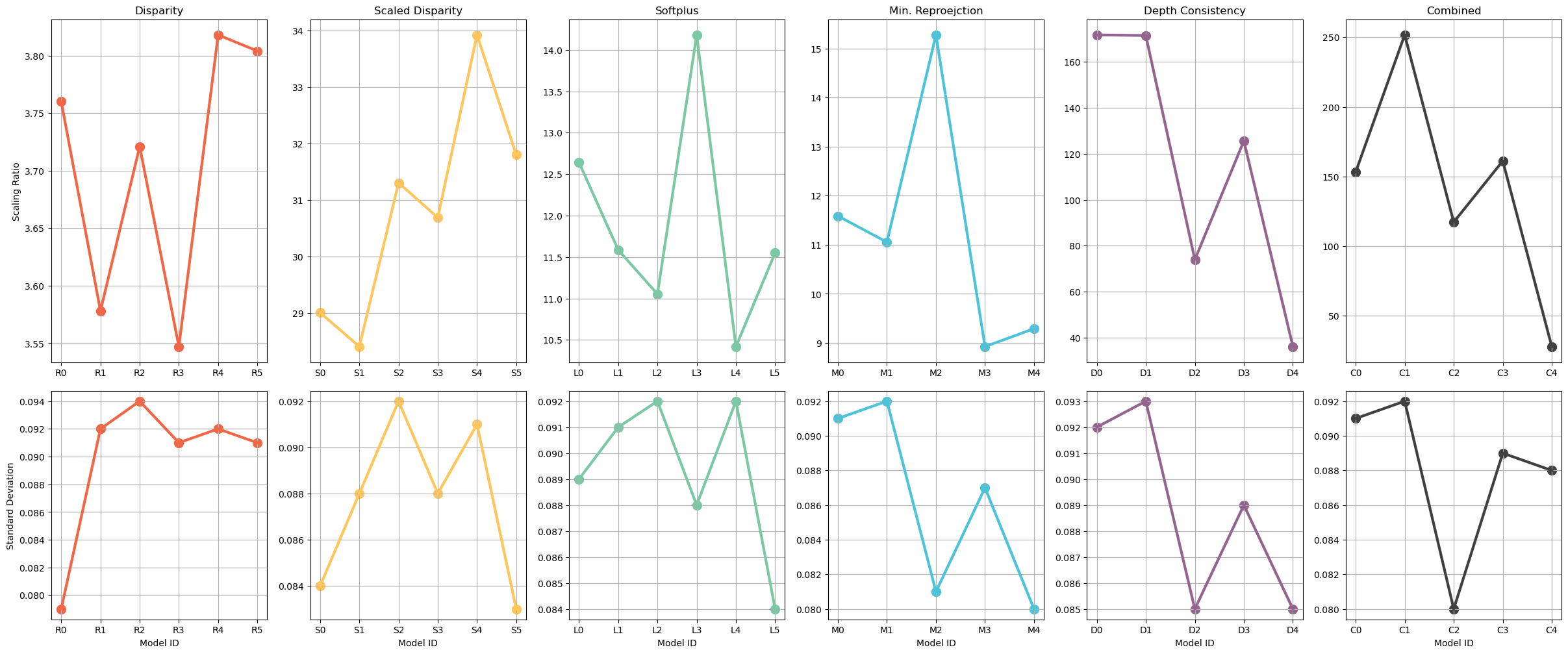
Figure 1: The scaling ratio and standard deviation of depth scales for each model. A large scaling ratio indicates small depth values learned, while a large standard deviation implies inconsistent-scale depth estimation. Compared to the ground-truth depth values, the models combining the MR loss and depth consistency learned much smaller depth values.

Better Depth Representation Exists. Table 2 summarizes the empirical study results. Among three depth representations considered in this study, the softplus representation displays superior performance. From R and S to L, the performance likely improves. This indicates that simple replacement of depth representation aids networks in learning better monocular depth estimation. Furthermore, the direct estimation of depth rather than the conventional disparity-based depth estimation shows improved performance. We presume that the softplus representation requiring zero hyper-parameters lets networks freely learn the optimal depth values. On the other hand, depth learning with the softplus representation diverged several times during our investigation, while the scaled disparity hardly showed such instability. This implies that there might exist trade-offs between representation power and learning stability at the current state.

Not All Approaches Are Universal. The effectiveness of several learning approaches depends on other learning approaches employed together. For instance, DW-SSIM is most effective with the disparity representation, while it does not evidently boost the performance for other representations (compare X2 and X4, where X$\in${R, S, L}). Further, the brightness transformation enhances the performance with the scaled disparity to a certain degree though it is not apparent for other representations (compare X1 and X3, where X$\in${R, S, L}). Similarly, the MR loss and DC adequately handle occlusions (compare L0 against M0 and D0) and the combination of the two methods seems to result in a synergy (compare M0 and D0 against C0), but the combination of the two methods does not display such synergy when associated with other learning approaches.

Auto-Mask and Motion Map Whenever Possible. These two approaches consistently enhance the monocular depth estimation performance (compare X0 against X1 and X3, where X$\in${M, D, C}). We suppose these two methods are complementary in dealing with dynamic objects since they target exclusive sets of dynamic objects: auto-masking copes with static scenes and objects moving with the same velocity as the camera, and motion map deals with objects with substantial movements. At this stage, we mark the M3 model as our baseline model for investigating the architectural impacts. One thing to note here is that we already remarkably enhanced the performance of the previous state-of-the-art model (S2) by properly shaping the learning configuration.

4.4 Architectural Impacts

Table 3 displays the effect of CNN architectures on monocular depth estimation performance. In the case of ResNet and DeResNet, the performance improves in the order of 18, 101 and 50 layers. This implies that merely scaling the network size does not result in performance enhancement. Moreover, the experiment results show that deformable convolutions definitely learn better features for depth estimation only when adequately placed (DeResNet-50): DeResNet-101 displays inferior performance than ResNet-101, while the performance degradation in DeResNet-18 can be attributed to unavailable pre-trained weights. The DeResNet-50 model once again boosts the depth estimation performance.

Next, EfficientNet-B0, B1 and B2 diverged within five epochs of training. We attempted to train the models multiple times with different learning parameters but only to fail in all cases. On the other hand, the learning process was stable for EfficientNet-B4—although its performance saturated within ten epochs of training. We assume that the EfficientNet architecture demands another training setting for stable depth learning. Taking the small numbers of training epochs into account, the performance of EfficientNets is moderate. In summary, the architectural factors require careful incorporation with other components similar to the learning approaches whose effectiveness depends on the learning configuration. We expect the application of recent advances in neural architecture search would even further enhance the performance.

4.5 Scale Consistency Analysis

Fig. 1 delineates the scaling ratios (SR) and standard deviations of SR of each model. Larger scaling ratios indicate smaller depth values learned compared to the ground-truth depth values. The scaled disparity representation makes networks learn smaller depth values (SR$\approx$31). This mechanism would stabilize the learning process. The disparity (SR$\approx$3.6) and softplus (SR$\approx$12) representations learn larger depth values than the scaled disparity representation. Furthermore, the MR loss does not dramatically vary the depth value range networks learn, whereas depth consistency makes networks learn much smaller depth values (compare the 3rd against 4th and 5th graphs). We would further investigate the relationship between the scales of depth values learned and the learning stability.

Besides, the standard deviation graphs share a similar structure. First, the two local maxima (X2 and X4, where X$\in${R, S, L}) in the disparity, scaled disparity and softplus graphs signal that the MR loss and AM increase the standard deviation while improving the depth estimation performance. Next, the uncertainty modeling shrinks the standard deviation while it does not significantly contribute to the depth learning (X2 and X4, where X$\in${M, D, C}). This trend could imply the trade-offs between performance and depth scale consistency.

5 Conclusion

In this work, we examined the self-supervised monocular depth and motion learning from previously unexplored angles. By designing a thorough empirical study, we revealed multiple essential insights: (1) better depth representation exists; thus, an appropriate choice of depth representation dramatically improves the performance, (2) not all learning approaches are universal, and they have their own effective setting, (3) the combination of auto-masking and motion map formulation consistently enhances the performance by handling dynamic objects, (4) CNN architectures do affect the performance substantially, and neural architecture search for self-supervised depth learning lingers, and (5) there might exist trade-offs between depth scale consistency and performance enhancement. Moreover, we obtained new state-of-the-art performance as a result of our study. Finally, we expect our extensive investigation has revealed crucial insights for future research directions for the corresponding research community.

Supplementary Material

Appendix A Qualitative Results

A.1 Motion Maps

Fig. 2 displays the motion maps estimated for the KITTI odometry dataset. The motion map compensates for large dynamic objects that are close to the camera. In addition, the motion map not only handles dynamic objects but also deals with the areas tricky for photometric reconstruction. For example, the motion map estimates motions for the areas with leaves or the part of buildings where the sun is shining down. These results imply that the motion map formulation aids the depth estimation network in learning to compensate for the violation of the implicit assumptions of the photometric consistency loss: the static scene assumption and the Lambertian surface assumption.

A.2 Depth Maps

Fig. 3 compares the depth maps estimated by our method to those of conventional methods. In most cases, the depth maps of the proposed method display more fine-grained structures of objects and scenes. Moreover, the depth maps of our method delineate the outline of dynamic objects such as humans and vehicles in a concrete manner. Compared to the interpolated ground-truth depth maps, the depth maps from the proposed method show continuous depth values without holes.

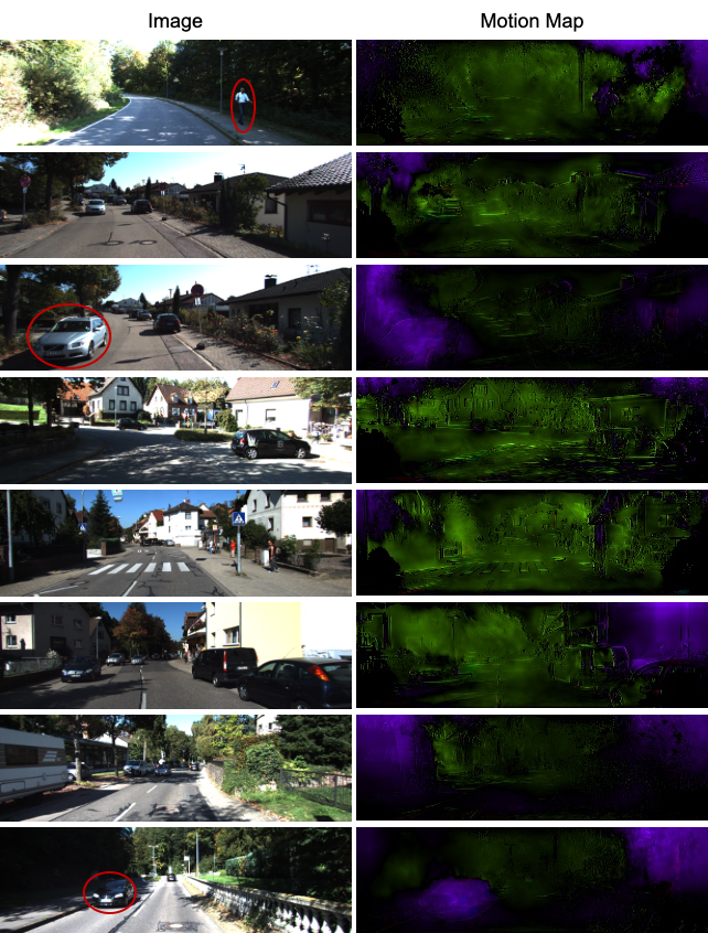
Figure 2: Visualization of the motion maps learned. The learned motion map compensates for large dynamic objects that are close to the camera. The red circles mark the dynamic objects in the scenes.

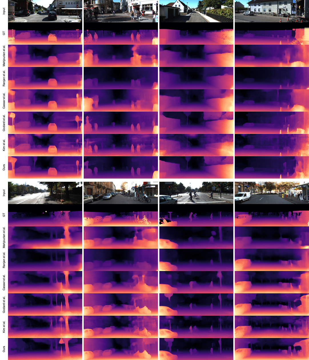
Figure 3: The qualitative comparison of depths maps. The depth maps of the proposed method clearly delineate the outlines of objects. Compared to the interpolated ground-truth depth maps, the proposed method provides continuous depth maps without holes. Moreover, the depth maps of the proposed method could handle the dynamic objects such as humans and vehicles.

Appendix B Comparative Study

Table 4 quantitatively compares the depth estimation results of the proposed method to conventional methods. Recent methods have employed either the DispNet architecture or the ResNet-18 architecture, while two of them employed ResNet-50 and ResNet-101. For a fair comparison, we indicate the architecture each method has employed. The proposed method displays superior or on-par performance compared to the state-of-the-art models according to the performance metrics. Here, we emphasize once again that the purpose of our study is to investigate (1) the inter-dependency between recent learning methods for self-supervised depth and motion learning and (2) the effect of architectural factors on performance. The performance gain followed as a result of our study. Besides, the need to search for the optimal architecture for self-supervised depth and motion learning lingers though we have investigated the architectural impact on the performance.

Table 4: Quantitative comparison results. The best results are in bold and the second best results are underlined. The proposed method displays superior or on-par performance compared to the state-of-the-art models.

Method	Architecture	ARD	SRD	RMSE	RMSE log	$\delta\!<\!1.25$	$\delta\!<\!1.25^{2}$	$\delta\!<\!1.25^{3}$
Mahjourian et al. [37]	DispNet [58]	0.163	1.240	6.220	0.250	0.762	0.916	0.968
Ranjan et al. [43]	DispNet [58]	0.148	1.149	5.464	0.226	0.815	0.935	0.973
Casser et al. [3]	ResNet-18	0.141	1.026	5.291	0.215	0.816	0.945	0.979
Godard et al. [11]	ResNet-18	0.115	0.903	4.863	0.193	0.877	0.959	0.981
Kim et al. [22]	ResNet-50	0.123	0.797	4.727	0.193	0.854	0.960	0.984
Johnston et al. [20]	ResNet-18	0.111	0.941	4.817	0.189	0.885	0.961	0.981
Johnston et al. [20]	ResNet-101	0.106	0.861	4.699	0.185	0.889	0.962	0.982
Ours	ResNet-18	0.114	0.825	4.706	0.191	0.877	0.960	0.982
Ours	DeResNet-50	0.108	0.737	4.562	0.187	0.883	0.961	0.982

References

- [1] Jiawang Bian, Zhichao Li, Naiyan Wang, Huangying Zhan, Chunhua Shen, Ming-Ming Cheng, and Ian Reid. Unsupervised scale-consistent depth and ego-motion learning from monocular video. In Advances in Neural Information Processing Systems (NeurIPS), volume 32, pages 35–45, 2019.
- [2] Léonard Blier and Yann Ollivier. The description length of deep learning models. In Advances in Neural Information Processing Systems (NeurIPS), pages 2220–2230, 2018.
- [3] Vincent Casser, Soeren Pirk, Reza Mahjourian, and Anelia Angelova. Depth prediction without the sensors: Leveraging structure for unsupervised learning from monocular videos. Proceedings of the AAAI Conference on Artificial Intelligence, 33(01):8001–8008, Jul. 2019.
- [4] Jifeng Dai, Haozhi Qi, Yuwen Xiong, Yi Li, Guodong Zhang, Han Hu, and Yichen Wei. Deformable convolutional networks. In Proceedings of the IEEE International Conference on Computer Vision (ICCV), pages 764–773, 2017.
- [5] David Eigen and Rob Fergus. Predicting depth, surface normals and semantic labels with a common multi-scale convolutional architecture. In Proceedings of the IEEE International Conference on Computer Vision (ICCV), pages 2650–2658, 2015.
- [6] David Eigen, Christian Puhrsch, and Rob Fergus. Depth map prediction from a single image using a multi-scale deep network. Advances in Neural Information Processing Systems (NeurIPS), 27:2366–2374, 2014.
- [7] Yarin Gal and Zoubin Ghahramani. Dropout as a bayesian approximation: Representing model uncertainty in deep learning. In International Conference on Machine Learning (ICML), pages 1050–1059. PMLR, 2016.
- [8] Andreas Geiger, Philip Lenz, Christoph Stiller, and Raquel Urtasun. Vision meets robotics: The kitti dataset. The International Journal of Robotics Research, 32(11):1231–1237, 2013.
- [9] Soumya Ghosh, Jiayu Yao, and Finale Doshi-Velez. Structured variational learning of bayesian neural networks with horseshoe priors. In International Conference on Machine Learning (ICML), pages 1744–1753. PMLR, 2018.
- [10] Clément Godard, Oisin Mac Aodha, and Gabriel J Brostow. Unsupervised monocular depth estimation with left-right consistency. In Proceedings of the IEEE Conference on Computer Vision and Pattern Recognition (CVPR), pages 270–279, 2017.
- [11] Clément Godard, Oisin Mac Aodha, Michael Firman, and Gabriel J Brostow. Digging into self-supervised monocular depth estimation. In Proceedings of the IEEE/CVF International Conference on Computer Vision (ICCV), pages 3828–3838, 2019.
- [12] Ariel Gordon, Hanhan Li, Rico Jonschkowski, and Anelia Angelova. Depth from videos in the wild: Unsupervised monocular depth learning from unknown cameras. In Proceedings of the IEEE/CVF International Conference on Computer Vision (ICCV), pages 8977–8986, 2019.
- [13] Alex Graves. Practical variational inference for neural networks. In Advances in Neural Information Processing Systems (NeurIPS), pages 2348–2356. Citeseer, 2011.
- [14] Kaiming He, Xiangyu Zhang, Shaoqing Ren, and Jian Sun. Deep residual learning for image recognition. In Proceedings of the IEEE Conference on Computer Vision and Pattern Recognition (CVPR), pages 770–778, 2016.
- [15] Andrew Howard, Mark Sandler, Grace Chu, Liang-Chieh Chen, Bo Chen, Mingxing Tan, Weijun Wang, Yukun Zhu, Ruoming Pang, Vijay Vasudevan, et al. Searching for mobilenetv3. In Proceedings of the IEEE/CVF International Conference on Computer Vision (ICCV), pages 1314–1324, 2019.
- [16] Jie Hu, Li Shen, and Gang Sun. Squeeze-and-excitation networks. In Proceedings of the IEEE Conference on Computer Vision and Pattern Recognition (CVPR), pages 7132–7141, 2018.
- [17] Yanping Huang, Youlong Cheng, Ankur Bapna, Orhan Firat, Mia Xu Chen, Dehao Chen, HyoukJoong Lee, Jiquan Ngiam, Quoc V Le, Yonghui Wu, et al. Gpipe: Efficient training of giant neural networks using pipeline parallelism. arXiv preprint arXiv:1811.06965, 2018.
- [18] Sergey Ioffe and Christian Szegedy. Batch normalization: Accelerating deep network training by reducing internal covariate shift. In International Conference on Machine Learning (ICML), pages 448–456. PMLR, 2015.
- [19] J Yu Jason, Adam W Harley, and Konstantinos G Derpanis. Back to basics: Unsupervised learning of optical flow via brightness constancy and motion smoothness. In Proceedings of the European Conference on Computer Vision (ECCV), pages 3–10. Springer, 2016.
- [20] Adrian Johnston and Gustavo Carneiro. Self-supervised monocular trained depth estimation using self-attention and discrete disparity volume. In Proceedings of the IEEE/CVF Conference on Computer Vision and Pattern Recognition (CVPR), pages 4756–4765, 2020.
- [21] Alex Kendall and Yarin Gal. What uncertainties do we need in bayesian deep learning for computer vision? In Advances in Neural Information Processing Systems (NeurIPS), page 5580–5590, Red Hook, NY, USA, 2017. Curran Associates Inc.
- [22] Ue-Hwan Kim, Seho Kim, and Jong-Hwan Kim. Simvodis: Simultaneous visual odometry, object detection, and instance segmentation. IEEE Transactions on Pattern Analysis and Machine Intelligence, 2020.
- [23] Diederik P Kingma and Jimmy Ba. Adam: A method for stochastic optimization. arXiv preprint arXiv:1412.6980, 2014.
- [24] Maria Klodt and Andrea Vedaldi. Supervising the new with the old: learning sfm from sfm. In Proceedings of the European Conference on Computer Vision (ECCV), pages 698–713, 2018.
- [25] Simon Kornblith, Jonathon Shlens, and Quoc V Le. Do better imagenet models transfer better? In Proceedings of the IEEE/CVF Conference on Computer Vision and Pattern Recognition (CVPR), pages 2661–2671, 2019.
- [26] Akio Kosaka and Avinash C Kak. Fast vision-guided mobile robot navigation using model-based reasoning and prediction of uncertainties. CVGIP: Image understanding, 56(3):271–329, 1992.
- [27] Alex Krizhevsky, Ilya Sutskever, and Geoffrey E Hinton. Imagenet classification with deep convolutional neural networks. Advances in Neural Information Processing Systems (NeurIPS), 25:1097–1105, 2012.
- [28] Yongchan Kwon, Joong-Ho Won, Beom Joon Kim, and Myunghee Cho Paik. Uncertainty quantification using bayesian neural networks in classification: Application to biomedical image segmentation. Computational Statistics & Data Analysis, 142:1–17, 2020.
- [29] Lubor Ladicky, Jianbo Shi, and Marc Pollefeys. Pulling things out of perspective. In Proceedings of the IEEE Conference on Computer Vision and Pattern Recognition (CVPR), pages 89–96, 2014.
- [30] Balaji Lakshminarayanan, Alexander Pritzel, and Charles Blundell. Simple and scalable predictive uncertainty estimation using deep ensembles. In Proceedings of the 31st International Conference on Neural Information Processing Systems (NeurIPS), page 6405–6416. Curran Associates Inc., 2017.
- [31] Congcong Li, Adarsh Kowdle, Ashutosh Saxena, and Tsuhan Chen. Towards holistic scene understanding: Feedback enabled cascaded classification models. In Advances in Neural Information Processing Systems (NeurIPS), pages 1351–1359, 2010.
- [32] Hanhan Li, Ariel Gordon, Hang Zhao, Vincent Casser, and Anelia Angelova. Unsupervised monocular depth learning in dynamic scenes. arXiv preprint arXiv:2010.16404, 2020.
- [33] Zhengqi Li, Tali Dekel, Forrester Cole, Richard Tucker, Noah Snavely, Ce Liu, and William T Freeman. Learning the depths of moving people by watching frozen people. In Proceedings of the IEEE/CVF Conference on Computer Vision and Pattern Recognition (CVPR), pages 4521–4530, 2019.
- [34] Chenxu Luo, Zhenheng Yang, Peng Wang, Yang Wang, Wei Xu, Ram Nevatia, and Alan Yuille. Every pixel counts++: Joint learning of geometry and motion with 3d holistic understanding. IEEE Transactions on Pattern Analysis and Machine Intelligence, 42(10):2624–2641, 2020.
- [35] Fangchang Ma, Guilherme Venturelli Cavalheiro, and Sertac Karaman. Self-supervised sparse-to-dense: Self-supervised depth completion from lidar and monocular camera. In 2019 International Conference on Robotics and Automation (ICRA), pages 3288–3295. IEEE, 2019.
- [36] Ningning Ma, Xiangyu Zhang, Hai-Tao Zheng, and Jian Sun. Shufflenet v2: Practical guidelines for efficient cnn architecture design. In Proceedings of the European conference on computer vision (ECCV), pages 116–131, 2018.
- [37] Reza Mahjourian, Martin Wicke, and Anelia Angelova. Unsupervised learning of depth and ego-motion from monocular video using 3d geometric constraints. In Proceedings of the IEEE Conference on Computer Vision and Pattern Recognition (CVPR), pages 5667–5675, 2018.
- [38] Yue Meng, Yongxi Lu, Aman Raj, Samuel Sunarjo, Rui Guo, Tara Javidi, Gaurav Bansal, and Dinesh Bharadia. Signet: Semantic instance aided unsupervised 3d geometry perception. In Proceedings of the IEEE/CVF Conference on Computer Vision and Pattern Recognition (CVPR), pages 9810–9820, 2019.
- [39] Andriy Mnih and Karol Gregor. Neural variational inference and learning in belief networks. In International Conference on Machine Learning (ICML), pages 1791–1799. PMLR, 2014.
- [40] Jishnu Mukhoti and Yarin Gal. Evaluating bayesian deep learning methods for semantic segmentation. arXiv preprint arXiv:1811.12709, 2018.
- [41] Vinod Nair and Geoffrey E Hinton. Rectified linear units improve restricted boltzmann machines. In Proceedings of the 27th International Conference on International Conference on Machine Learning (ICML), pages 807–814, 2010.
- [42] Matteo Poggi, Filippo Aleotti, Fabio Tosi, and Stefano Mattoccia. On the uncertainty of self-supervised monocular depth estimation. In Proceedings of the IEEE/CVF Conference on Computer Vision and Pattern Recognition (CVPR), pages 3227–3237, 2020.
- [43] Anurag Ranjan, Varun Jampani, Lukas Balles, Kihwan Kim, Deqing Sun, Jonas Wulff, and Michael J Black. Competitive collaboration: Joint unsupervised learning of depth, camera motion, optical flow and motion segmentation. In Proceedings of the IEEE Conference on Computer Vision and Pattern Recognition (CVPR), pages 12240–12249, 2019.
- [44] Zhe Ren, Junchi Yan, Bingbing Ni, Bin Liu, Xiaokang Yang, and Hongyuan Zha. Unsupervised deep learning for optical flow estimation. Proceedings of the AAAI Conference on Artificial Intelligence, 31(1):1495–1501, 2017.
- [45] Hippolyt Ritter, Aleksandar Botev, and David Barber. A scalable laplace approximation for neural networks. In 6th International Conference on Learning Representations, ICLR 2018-Conference Track Proceedings, volume 6. International Conference on Representation Learning, 2018.
- [46] Mark Sandler, Andrew Howard, Menglong Zhu, Andrey Zhmoginov, and Liang-Chieh Chen. Mobilenetv2: Inverted residuals and linear bottlenecks. In Proceedings of the IEEE Conference on Computer Vision and Pattern Recognition (CVPR), pages 4510–4520, 2018.
- [47] Ashutosh Saxena, Min Sun, and Andrew Y Ng. Make3d: Learning 3d scene structure from a single still image. IEEE Transactions on Pattern Analysis and Machine Intelligence, 31(5):824–840, 2008.
- [48] Christian Szegedy, Wei Liu, Yangqing Jia, Pierre Sermanet, Scott Reed, Dragomir Anguelov, Dumitru Erhan, Vincent Vanhoucke, and Andrew Rabinovich. Going deeper with convolutions. In Proceedings of the IEEE Conference on Computer Vision and Pattern Recognition (CVPR), pages 1–9, 2015.
- [49] Richard Szeliski. Bayesian modeling of uncertainty in low-level vision. International Journal of Computer Vision, 5(3):271–301, 1990.
- [50] Mingxing Tan, Bo Chen, Ruoming Pang, Vijay Vasudevan, Mark Sandler, Andrew Howard, and Quoc V Le. Mnasnet: Platform-aware neural architecture search for mobile. In Proceedings of the IEEE/CVF Conference on Computer Vision and Pattern Recognition (CVPR), pages 2820–2828, 2019.
- [51] Mingxing Tan and Quoc Le. Efficientnet: Rethinking model scaling for convolutional neural networks. In International Conference on Machine Learning (ICML), pages 6105–6114. PMLR, 2019.
- [52] Alvin Wan, Xiaoliang Dai, Peizhao Zhang, Zijian He, Yuandong Tian, Saining Xie, Bichen Wu, Matthew Yu, Tao Xu, Kan Chen, et al. Fbnetv2: Differentiable neural architecture search for spatial and channel dimensions. In Proceedings of the IEEE/CVF Conference on Computer Vision and Pattern Recognition (CVPR), pages 12965–12974, 2020.
- [53] Rui Wang, Martin Schworer, and Daniel Cremers. Stereo dso: Large-scale direct sparse visual odometry with stereo cameras. In Proceedings of the IEEE International Conference on Computer Vision (ICCV), pages 3903–3911, 2017.
- [54] Nan Yang, Lukas von Stumberg, Rui Wang, and Daniel Cremers. D3vo: Deep depth, deep pose and deep uncertainty for monocular visual odometry. In Proceedings of the IEEE/CVF Conference on Computer Vision and Pattern Recognition (CVPR), pages 1281–1292, 2020.
- [55] Tien-Ju Yang, Andrew Howard, Bo Chen, Xiao Zhang, Alec Go, Mark Sandler, Vivienne Sze, and Hartwig Adam. Netadapt: Platform-aware neural network adaptation for mobile applications. In Proceedings of the European Conference on Computer Vision (ECCV), pages 285–300, 2018.
- [56] Zhichao Yin and Jianping Shi. Geonet: Unsupervised learning of dense depth, optical flow and camera pose. In Proceedings of the IEEE Conference on Computer Vision and Pattern Recognition (CVPR), pages 1983–1992, 2018.
- [57] Chris Ying, Aaron Klein, Eric Christiansen, Esteban Real, Kevin Murphy, and Frank Hutter. Nas-bench-101: Towards reproducible neural architecture search. In International Conference on Machine Learning (ICML), pages 7105–7114. PMLR, 2019.
- [58] Tinghui Zhou, Matthew Brown, Noah Snavely, and David G Lowe. Unsupervised learning of depth and ego-motion from video. In Proceedings of the IEEE Conference on Computer Vision and Pattern Recognition (CVPR), pages 1851–1858, 2017.
- [59] Xizhou Zhu, Han Hu, Stephen Lin, and Jifeng Dai. Deformable convnets v2: More deformable, better results. In Proceedings of the IEEE/CVF Conference on Computer Vision and Pattern Recognition (CVPR), pages 9308–9316, 2019.
- [60] Yuliang Zou, Zelun Luo, and Jia-Bin Huang. Df-net: Unsupervised joint learning of depth and flow using cross-task consistency. In Proceedings of the European Conference on Computer Vision (ECCV), pages 36–53, 2018.